
Review: Dynamic ProgrammingReview: Dynamic Programming
• Dynamic Programming is a technique for algorithm
design. It is a tabular method in which we break down the
problem into subproblems, and place the solution to the
subproblems in a matrix. The matrix elements can be
computed:
– iteratively, in a bottom-up fashion;
– recursively, using memoization.
• Dynamic Programming is often used to solve
optimization problems. In these cases, the solution
corresponds to an objective function whose value needs to
be optimal (e.g. maximal or minimal). Usually it is
sufficient to produce one optimal solution, even though
there may be many optimal solutions for a given problem.
'
&
$
%CS404/504 Computer Science
1Design and Analysis of Algorithms: Lecture 17

Developing Dynamic ProgrammingAlgorithms
Developing Dynamic ProgrammingAlgorithms
Four steps:
(i) Characterize the structure of an optimal solution.
(ii) Recursively define the value of an optimal solution.
(iii) Compute the value of an optimal solution in a bottom
up fashion.
(iv) Construct an optimal solution from the computed
information.
'
&
$
%CS404/504 Computer Science
2Design and Analysis of Algorithms: Lecture 17

Matrix Chain MultiplicationMatrix Chain Multiplication
Basics
Let A be a p × q matrix and let B be a q × r matrix. Then
we can multiply Ap×q ∗ Bq×r = Cp×r, where the elements of
Cp×r are defined as:
cij =q
∑
k=1
aikbkj
The straightforward algorithm to compute Ap×q ∗ Bq×r
takes p ∗ q ∗ r multiplications.
Chains of Matrices
Consider A1 · A2 · ... · An. We can compute this product if
the number of columns in Ai is equal to the number of rows
in Ai+1 (Cols[Ai] =Rows[Ai+1]) for every 1 ≤ i ≤ n − 1.
'
&
$
%CS404/504 Computer Science
3Design and Analysis of Algorithms: Lecture 17
How to order the multiplications?How to order the multiplications?
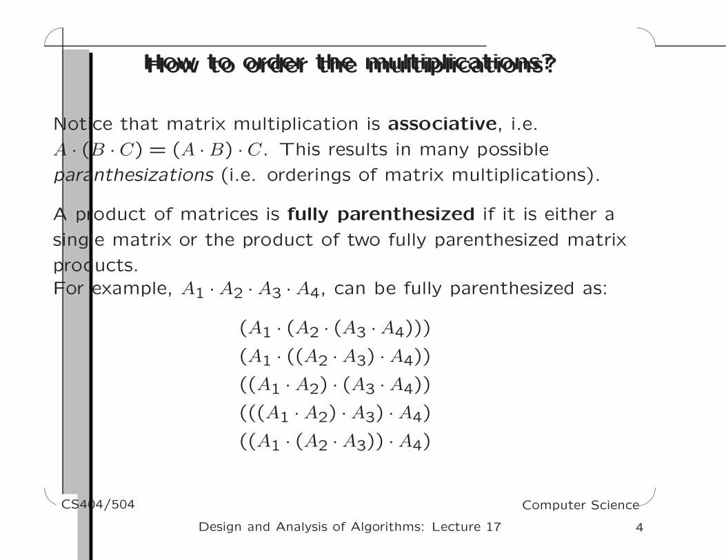
Notice that matrix multiplication is associative, i.e.
A · (B · C) = (A · B) · C. This results in many possible
paranthesizations (i.e. orderings of matrix multiplications).
A product of matrices is fully parenthesized if it is either a
single matrix or the product of two fully parenthesized matrix
products.
For example, A1 · A2 · A3 · A4, can be fully parenthesized as:
(A1 · (A2 · (A3 · A4)))
(A1 · ((A2 · A3) · A4))
((A1 · A2) · (A3 · A4))
(((A1 · A2) · A3) · A4)
((A1 · (A2 · A3)) · A4)
'
&
$
%CS404/504 Computer Science
4Design and Analysis of Algorithms: Lecture 17
The parenthesization is importantThe parenthesization is important
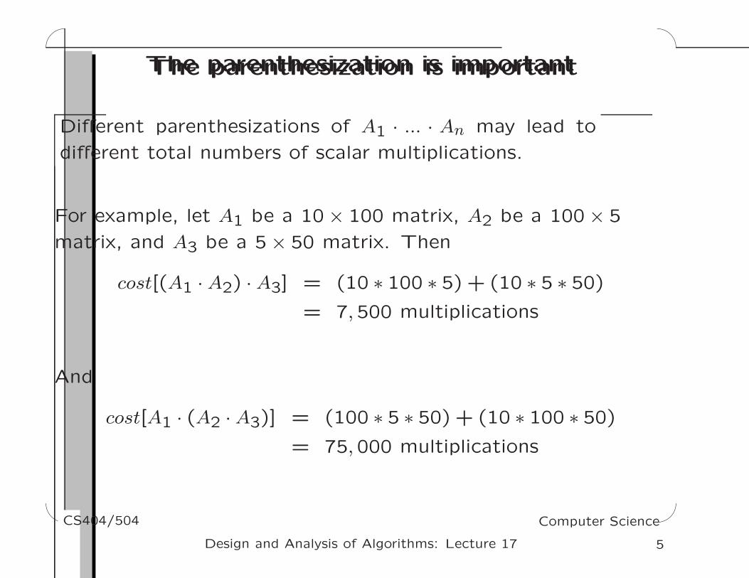
Different parenthesizations of A1 · ... · An may lead to
different total numbers of scalar multiplications.
For example, let A1 be a 10 × 100 matrix, A2 be a 100 × 5
matrix, and A3 be a 5 × 50 matrix. Then
cost[(A1 · A2) · A3] = (10 ∗ 100 ∗ 5) + (10 ∗ 5 ∗ 50)
= 7,500 multiplications
And
cost[A1 · (A2 · A3)] = (100 ∗ 5 ∗ 50) + (10 ∗ 100 ∗ 50)
= 75,000 multiplications
'
&
$
%CS404/504 Computer Science
5Design and Analysis of Algorithms: Lecture 17

There are Ω(2n) possible parenthesizationsThere are Ω(2n) possible parenthesizations
We can think of a parenthesization as a binary parse tree.
Examples:
– left-branching: ((...((A1 · A2) · A3)...) · An)
– right-branching: (A1 · (...(An−2 · (An−1 · An))...))
Total number of paranthesizations is:
P(n) =
1 if n = 1,n−1∑
k=1
P(k)P(n − k) if n ≥ 2.
P(n) is the sequence of Catalan numbers, which grows as
Ω(2n) (Exercise 15.2-3) ⇒ Brute force is ruled out!
'
&
$
%CS404/504 Computer Science
6Design and Analysis of Algorithms: Lecture 17

The Matrix Chain Multiplication ProblemThe Matrix Chain Multiplication Problem
Input:
A chain of n matrices 〈A1, A2, ..., An〉 such that
Cols[Ai] =Rows[Ai+1], for i = 1,2, ..., n
Output:
An optimal, fully parenthesized product A1 ·A2 · ... ·An (i.e., in a
way that minimizes the total number of scalar multiplications).
'
&
$
%CS404/504 Computer Science
7Design and Analysis of Algorithms: Lecture 17

A Dynamic Programming Solution: Step (i)A Dynamic Programming Solution: Step (i)
Step (i) characterize the structure of an optimal solution.
Assume that the optimal way to multiply A1A2......An is
(A1A2...Ak)(Ak+1...An), for some k.
Its associated cost is:
cost(A1...An) = cost(A1...Ak) + cost(Ak+1...An) +
rows[A1] · col[Ak] · col[An] (1)
If cost(A1...An) is minimal, then both both cost(A1...Ak) and
cost(Ak+1...An) are minimal. Why?
'
&
$
%CS404/504 Computer Science
8Design and Analysis of Algorithms: Lecture 17
A Dynamic Programming Solution: Step (ii)A Dynamic Programming Solution: Step (ii)
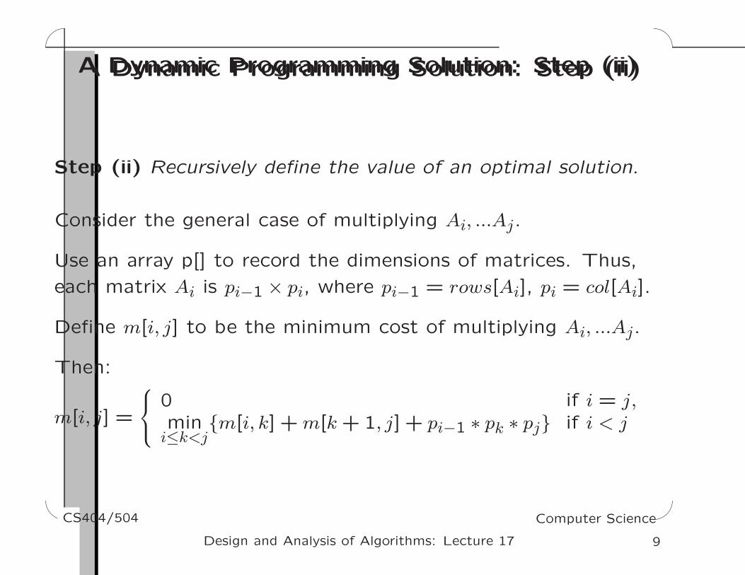
Step (ii) Recursively define the value of an optimal solution.
Consider the general case of multiplying Ai, ...Aj.
Use an array p[] to record the dimensions of matrices. Thus,
each matrix Ai is pi−1 × pi, where pi−1 = rows[Ai], pi = col[Ai].
Define m[i, j] to be the minimum cost of multiplying Ai, ...Aj.
Then:
m[i, j] =
0 if i = j,
mini≤k<j
m[i, k] + m[k + 1, j] + pi−1 ∗ pk ∗ pj if i < j
'
&
$
%CS404/504 Computer Science
9Design and Analysis of Algorithms: Lecture 17

Compute m[i,j]: A Simple Recursive ApproachCompute m[i,j]: A Simple Recursive Approach
Directly compute m[i, j] based on the recursive solution:
RECURSIVE-MATRIX-CHAIN (p, i, j)
if i = j return 0;
m[i, j] := ∞;
for k := i to j − 1
q := RECURSIVE-MATRIX-CHAIN (p, i, k)
+ RECURSIVE-MATRIX-CHAIN (p, k + 1, j)
+ pi−1 · pk · pj
if q < m[i, j]
m[i, j] := q;
return m[i, j]
'
&
$
%CS404/504 Computer Science
10Design and Analysis of Algorithms: Lecture 17

Recursive-Matrix-Chain(p, 1, 4)Recursive-Matrix-Chain(p, 1, 4)
'
&
$
%CS404/504 Computer Science
11Design and Analysis of Algorithms: Lecture 17

Time AnalysisTime Analysis
The following recurrence relation describes the running time of
RECURSIVE-MATRIX-CHAIN():
T(1) ≥ 1
T(n) ≥ 1 +n−1∑
k=1
(T(k) + T(n − k) + 1)
= 2n−1∑
i=1
T(i) + n
Exercise
Prove that T(n) ≥ 2n−1
'
&
$
%CS404/504 Computer Science
12Design and Analysis of Algorithms: Lecture 17

Compute m[i,j]: A Bottom-Up IterativeApproach
Compute m[i,j]: A Bottom-Up IterativeApproach
We can compute m[1..n] in O(n3) steps.
'
&
$
%CS404/504 Computer Science
13Design and Analysis of Algorithms: Lecture 17

Bottom-Up Iterative ExampleBottom-Up Iterative Example
Example:
A1 30x35
A2 35x15
A3 15x5
A4 5x10
A5 10x20
A6 20x25
Let’s fill in part of the m array for this example.
'
&
$
%CS404/504 Computer Science
14Design and Analysis of Algorithms: Lecture 17

Bottom-Up Iterative ExampleBottom-Up Iterative Example
'
&
$
%CS404/504 Computer Science
15Design and Analysis of Algorithms: Lecture 17

Working it outWorking it out
m[2,6] = min2≤k≤6
m[2, k] + m[k + 1,6] + p1 · pk · p6
= min
m[2,2] + m[3,6] + 35 × 15 × 25 = 18,500m[2,3] + m[4,6] + 35 × 5 × 25 = 10,510m[2,4] + m[5,6] + 35 × 10 × 25 = 18,125m[2,5] + m[6,6] + 35 × 20 × 25 = 24,625
Thus, S[2,6] = k = 3.
'
&
$
%CS404/504 Computer Science
16Design and Analysis of Algorithms: Lecture 17
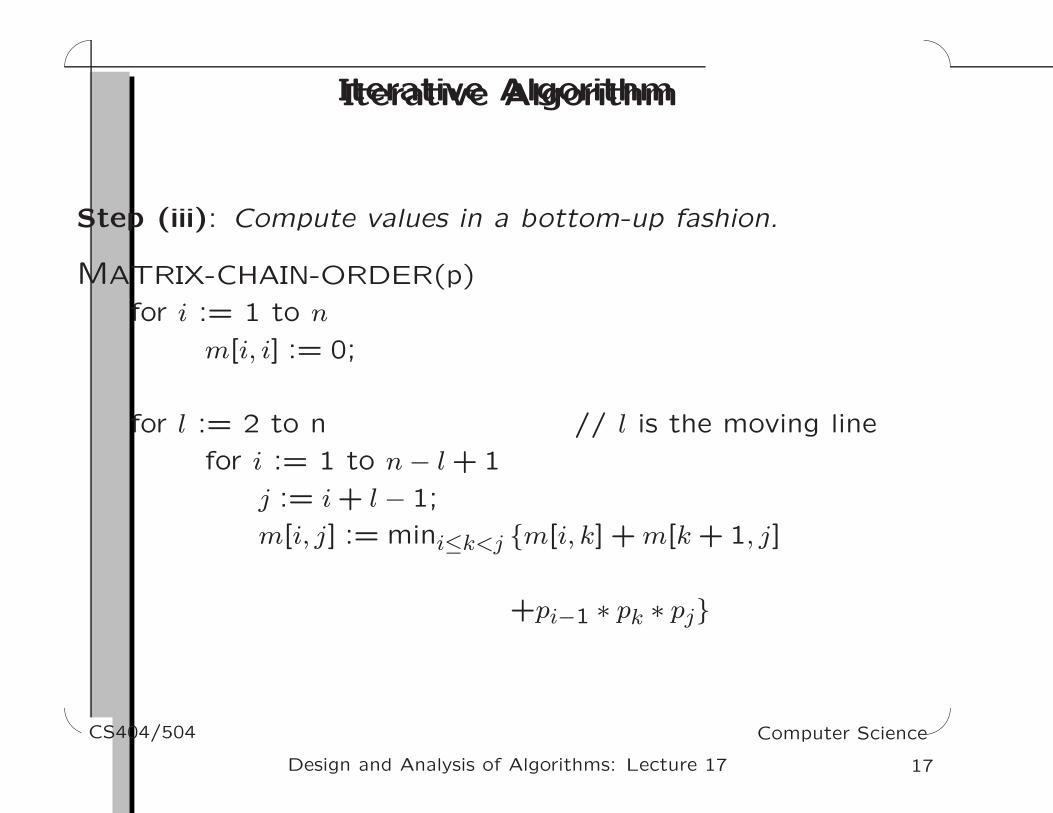
Iterative AlgorithmIterative Algorithm
Step (iii): Compute values in a bottom-up fashion.
MATRIX-CHAIN-ORDER(p)
for i := 1 to n
m[i, i] := 0;
for l := 2 to n // l is the moving line
for i := 1 to n − l + 1
j := i + l − 1;
m[i, j] := mini≤k<j m[i, k] + m[k + 1, j]
+pi−1 ∗ pk ∗ pj
'
&
$
%CS404/504 Computer Science
17Design and Analysis of Algorithms: Lecture 17

Complexity is Θ(n3)Complexity is Θ(n3)
MATRIX-CHAIN-ORDER(p)
for i := 1 to n Θ(n)
m[i, i] := 0;
for l := 2 to n O(n)
for i := 1 to n − l + 1 O(n)
j := i + l − 1;
m[i, j] := mini≤k<j m[i, k] + m[k + 1, j] O(n)
+pi−1 ∗ pk ∗ pj
Overal: O(n3). It’s also Ω(n3) (homework).
'
&
$
%CS404/504 Computer Science
18Design and Analysis of Algorithms: Lecture 17

Step (iv): Constructing an optimal solutionStep (iv): Constructing an optimal solution
Use another table s[1..n,1..n]. Each entry s[i, j] records the
value of k such that the optimal parenthesization of AiAi+1...Aj
splits the product between Ak and Ak+1.
MATRIX-CHAIN-ORDER(p)
for l := 2 to n
for i := 1 to n − l + 1
j := i + l − 1;
m[i, j] := mini≤k<j
m[i, k] + m[k + 1, j] + pi−1 ∗ pk ∗ pj
s[i, j] := argmini≤k<j
m[i, k] + m[k + 1, j] + pi−1 ∗ pk ∗ pj
'
&
$
%CS404/504 Computer Science
19Design and Analysis of Algorithms: Lecture 17

Step (iv): Constructing an optimal solutionStep (iv): Constructing an optimal solution
How do we find the actual optimal parenthesization?
Notice that s[1, n] is the position of the outmost multiplication.
(A1...As[1,n])(As[1,n]+1)....An)
Similarly, the outermost multiplication for the left-hand side is
at the position s[1, s[1, n]], and the outermost multiplication for
the right-hand side is at the position s[s[1, n] + 1, n].
We can generalize this to give a simple recursive algorithm to
print the minimal parenthesization.
'
&
$
%CS404/504 Computer Science
20Design and Analysis of Algorithms: Lecture 17
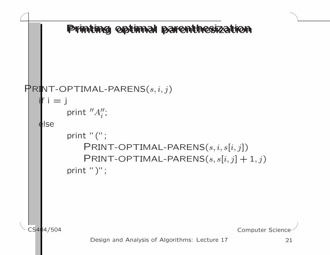
Printing optimal parenthesizationPrinting optimal parenthesization
PRINT-OPTIMAL-PARENS(s, i, j)
if i = j
print ′′A′′i ;
else
print ”(”;
PRINT-OPTIMAL-PARENS(s, i, s[i, j])
PRINT-OPTIMAL-PARENS(s, s[i, j] + 1, j)
print ”)”;
'
&
$
%CS404/504 Computer Science
21Design and Analysis of Algorithms: Lecture 17
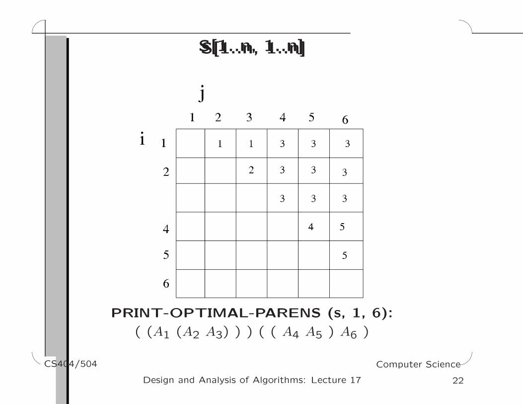
S[1..n, 1..n]S[1..n, 1..n]
PRINT-OPTIMAL-PARENS (s, 1, 6):
( (A1 (A2 A3) ) ) ( ( A4 A5 ) A6 )
'
&
$
%CS404/504 Computer Science
22Design and Analysis of Algorithms: Lecture 17

The Recursive Approach RevisitedThe Recursive Approach Revisited
As we’ve seen already, we can solve the matrix chain
multiplication problem recursively using the following algorithm:
RECURSIVE-MATRIX-CHAIN (p, i, j)
if i = j return 0;
m[i, j] := ∞;
for k := i to j − 1
q := RECURSIVE-MATRIX-CHAIN (p, i, k)
+ RECURSIVE-MATRIX-CHAIN (p, k + 1, j)
+ pi−1 · pk · pj
if q < m[i, j]
m[i, j] := q;
return m[i, j]
'
&
$
%CS404/504 Computer Science
23Design and Analysis of Algorithms: Lecture 17
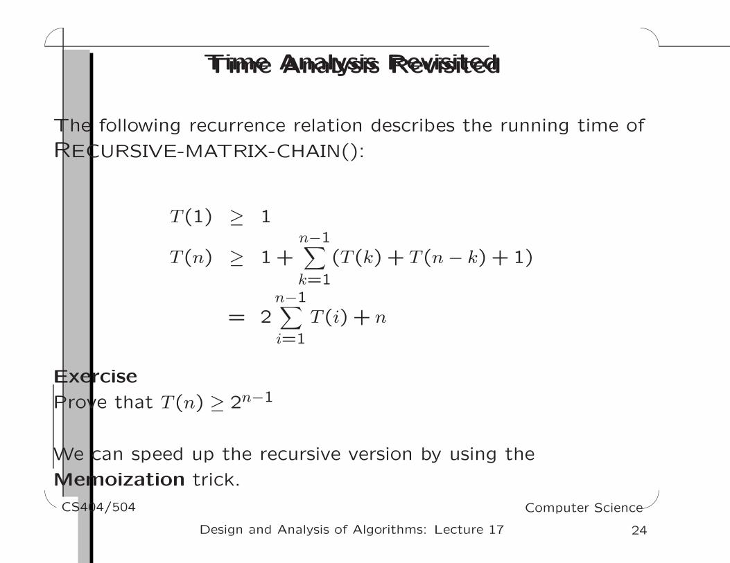
Time Analysis RevisitedTime Analysis Revisited
The following recurrence relation describes the running time of
RECURSIVE-MATRIX-CHAIN():
T(1) ≥ 1
T(n) ≥ 1 +n−1∑
k=1
(T(k) + T(n − k) + 1)
= 2n−1∑
i=1
T(i) + n
Exercise
Prove that T(n) ≥ 2n−1
We can speed up the recursive version by using the
Memoization trick.
'
&
$
%CS404/504 Computer Science
24Design and Analysis of Algorithms: Lecture 17

Memoization (pages 387–389)Memoization (pages 387–389)
We can make the recursive version more efficient than the
straightforward approach that we gave earlier.
Basic Idea: Since the recursive version recomputes many of
it’s values, we can simply “remember” the values that we’ve
already computed, and not recompute them.
Notice that this requires that we save some extra information
to tell us that we have already computed some value.
We can create a memoized version for the matrix chain
problem.
'
&
$
%CS404/504 Computer Science
25Design and Analysis of Algorithms: Lecture 17

Memoized Matrix ChainMemoized Matrix Chain
Memoized-Matrix-Chain (p)
Initialization();
Lookup-Chain(p,1, n);
First, we set all of the values m[i, j] = ∞ to indicate that they
have not been computed, yet.
Initialization()
for i = 1 to n do
for j = i to n do
m[i, j] = ∞;
'
&
$
%CS404/504 Computer Science
26Design and Analysis of Algorithms: Lecture 17

Memoized Matrix Chain: RecursionMemoized Matrix Chain: Recursion
Lookup-Chain (p, i, j)
if m[i, j] < ∞
return m[i, j];
if (i = j)
m[i, j] := 0;
else
for k := i to j − 1
q := Lookup-Chain (p, i, k) + Lookup-Chain (p, k + 1, j)
+ pi−1 · pk · pj;
if q < m[i, j]
m[i, j] := q;
return m[i, j]
'
&
$
%CS404/504 Computer Science
27Design and Analysis of Algorithms: Lecture 17

Advantages?Advantages?
Memoization gives an algorithm that is roughly as fast as the
iterative version – in practice it is slower by a constant factor,
due to the recursion overhead and table maintenance.
Think of how to analyze this algorithm – notice that the
standard recurrence relation analysis cannot be used.
Advantages of memoization:
– It is easier to code than the iterative version, thus it is less
error prone.
– It solves only those subproblems that are definitely required
(useful when not all subproblems in the subproblem space
need to be solved).
'
&
$
%CS404/504 Computer Science
28Design and Analysis of Algorithms: Lecture 17
Dynamic Programming: Key IngredientsDynamic Programming: Key Ingredients
Two ingredients of optimization problems that lead to a
dynamic programming solution:
• Optimal substructure: an optimal solution to the problem
contains within it optimal solutions to sub-problems.
• Overlapping sub-problems: same subproblem will be
visited again and again (i.e. subproblems share
subsubproblems).
'
&
$
%CS404/504 Computer Science
29Design and Analysis of Algorithms: Lecture 17

An example where optimal sub-structuredoesn’t hold
An example where optimal sub-structuredoesn’t hold
Longest Simple Path problem:
A directed graph showing that the problem of finding a longest
simple path in an unweighted directed graph does not have
optimal substructure.
The path q → r → t is a longest simple path from q to r, but
the subpath r → t is not a longest simple path from r to t.
'
&
$
%CS404/504 Computer Science
30Design and Analysis of Algorithms: Lecture 17
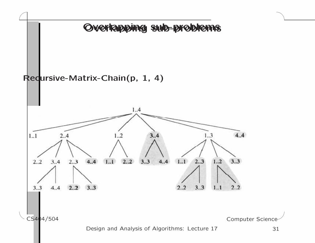
Overlapping sub-problemsOverlapping sub-problems
Recursive-Matrix-Chain(p, 1, 4)
'
&
$
%CS404/504 Computer Science
31Design and Analysis of Algorithms: Lecture 17

Overlapping sub-problemsOverlapping sub-problems
Fibonacci numbers:
F(100) = F(99) + F(98)
= (F(98) + F(97)) + ( F(97) + F(96))
= ...
'
&
$
%CS404/504 Computer Science
32Design and Analysis of Algorithms: Lecture 17
Divide & Conquer vs. Dynamic ProgrammingDivide & Conquer vs. Dynamic Programming
• Divide & Conquer is indicated when the sub-problems are
independent.
• Dynamic Programming is indicated when the sub-problems
share common sub-sub-problems.
'
&
$
%CS404/504 Computer Science
33Design and Analysis of Algorithms: Lecture 17

Greedy Method vs. Dynamic ProgrammingGreedy Method vs. Dynamic Programming
• Both require the solution of the optimization problem to
have optimal substructure.
• In Dynamic Programming, the optimal solution of a problem
depends on the optimal solution of its sub-problems, so the
computation is carried out in a bottom-up manner.
• In the Greedy method, a decision is made at each step
before solving the subproblem, so a greedy algorithm
usually runs in a top-down fashion.
• Greedy method uses only local information to make
decision. We need to prove that locally optimal decisions
lead to a globally optimal solution, and this is where
cleverness may be required.
'
&
$
%CS404/504 Computer Science
34Design and Analysis of Algorithms: Lecture 17


