
Preliminary and Incomplete
Risk and Robustness in General Equilibrium
Evan W. Anderson
Lars Peter Hansen
and
Thomas J. Sargent
March 8, 1998
1. Introduction
A ‘robust decision maker’ suspects that his model is misspecified and makes decisions
that work well over a restricted range of specification errors around a base or ‘reference’
model. In the context of a discrete time linear-quadratic permanent income model,
Hansen, Sargent and Tallarini (1997) (HST) used a single parameter – taken from a
version of Jacobson and Whittle’s ‘risk-sensitivity’ correction – to index the class of
relevant model misspecifications from which the decision maker seeks protection. In that
setting, HST showed how robust decision making would generate behavior that looks like
risk aversion. HST calculated how much ‘preference for robustness’ – interpreted as a
form of aversion to a particular kind of Knightian uncertainty – it takes to put ‘market
prices of risk’ into empirically plausible regions.
This paper extends the analysis of HST to economies with equilibrium allocations
that solve continuous time optimal resource allocation problems. Most of our results
exploit the analytical convenience of continuous-time diffusions. Working in continuous
time lets us leave the confines of a linear-quadratic framework: objective functions can
be nonquadratic and state evolution equations can be nonlinear. Leaving the linear-
quadratic framework makes it easier to link our robustness parameter to commonly used
measures of risk aversion both in decision problems and in security market data. It also
1

gives us a general characterization of a precautionary mechanism in decision-making
induced by a concern for robustness.
Previously, Epstein and Zin (1989) and Duffie and Epstein (1992) broke the link be-
tween intertemporal substitution and risk by introducing risk adjustments in evaluating
future utility indices. We demonstrate that concerns about robustness can imitate risk
aversion in decision-making in two ways. First we reinterpret one of Epstein-Zin’s (1989)
recursions as reflecting a preference for robustness rather than aversion to risk. Then
we recast the resulting (shadow) market price of risk partly as a ‘specification-error’ or
‘model uncertainty’ premium.
We motivate robustness by specifying a ‘reference model’ and particular nearby mod-
els. The decision maker specifies a family of ‘candidate’ nearby models. Looking at these
nearby models is the decision maker’s response to his suspicion that the reference model is
‘misspecified.’ We measure the discrepancy between the reference model and the nearby
models by using relative entropy, an expected log likelihood ratio, where the expectation
is taken over the distribution from the candidate nearby model. Relative entropy is a
key tool in the theory of large deviations, a powerful mathematical theory about rates
at which initially unknown distributions can be learned from empirical evidence.
Superficially at least, the perspective of the ‘robust’ controller differs substantially
from that of a ‘learner’. In our dynamic settings, the robust decision maker accepts
the presence of model misspecification as a permanent state of affairs, and devotes his
thoughts to designing robust controls, rather than, say, thinking about recursive ways
to use data to improve his model specification over time. But as we shall see, the
same formulas that in large deviation theory underpin theories of ‘learning’ also give
representations of value functions appropriate for robust decision making. ‘Learning’
and ‘robust decision’ share a need for a convenient way of measuring and interpreting
the proximity of two probability distributions, despite the differing orientations – of the
robust decision maker to ‘plan against the worst’, and of the learner to collect enough
data to decide. In our settings the robust decision maker is just being sensible in planning
against model misspecification that a ‘learner’ could not confidently dispose of even after
many observations.
2

2. Misspecification in Discrete Time
In this section we ignore the choice of the control and study an exogenous state evo-
lution equation. We consider first a Markov process for the state vector in either discrete
or continuous time. This process can be modeled by specifying a family (semigroup) of
conditional expectation operators:
Ts (φ) (y) = E [φ (xs) |x0 = y]
where the index s ranges over nonnegative numbers when time is continuous and over
nonnegative integers when time is discrete. The domain of the conditional expectation
operators contains at least the space of bounded, continuous functions. It typically can
be expanded to a larger space, but the manner in which it is done depends processes
being modeled. Such extensions are germaine to our analysis because we apply the
conditional expectation operators to value functions, which for some control problems
can be unbounded.
Given a current-period reward function, to compute a value function for a fixed
Markov process under discounting, one solves the fixed-point problem:
V (x) = sU (x) + exp (−sδ) TsV (x)
where U is a current period reward function, δ is the subjective rate of discount, s is the
period length, and V is the corresponding value function. Recursive utility formulations
generalize this fixed point problem by replacing Ts with an alternative transformation of
the value function, which we denote Rs. We aim to motivate a particular specification of
Rs incorporating a wish for robustness. Our notion of robustness is represented with a
class of conditional expectation operators for nearby perturbations of the original Markov
process for the state evolution.
For the remainder of this section, we consider misspecification of a discrete-time
process, taking the time increment to be unity. We start with a ‘reference process’
interpreted as a model that is to be treated only as a ‘good approximation’ of a possibly
more complicated model. People agree on the ‘reference model’ perhaps based on having
observed common historical data. They also worry about a common class of potential
misspecifications in the form of perturbations about the reference model. Agreement
3

about the reference model and the potential misspecifications is like imposing ‘rational
expectations’ in our framework.
In this section, the ‘reference model’ is specified as a discrete-time Markov process.
In discrete time it suffices to specify the one-period conditional expectation operator:
T1 ≡ T . Given the Markov structure, the remaining conditional expectation operators
can be constructed via the formula:
Tj = (T )j
for integer j. The operator T , or the corresponding Markov transition density, forms
our ‘reference model.’
To characterize model misspecification, we introduce a family of ‘candidate models.’
Concern for misspecification of a reference model is reflected by allowing discrepancies
between a permissible candidate model and the reference model, and somehow evaluating
utility over a collection of candidate models.
2.1. Markov Perturbations
We start by introducing a particularly simple family of candidate models and discuss
later what happens when we enrich this class. Our simple starting point by design
imitates a formalization used in large deviation theory for Markov processes (e.g. see
Dupuis and Ellis, 1997). We generate a class of candidate models, in the form of a simple
alteration of the reference model’s Markov process. For a strictly positive function w,
we form a distorted expectation operator:
T w (φ) =T (wφ)
T (w).
The operator T w gives rise to an alternative Markov specification for the state evolu-
tion.1
Given this construction, w(z)T (w)(y) is the Radon-Nikodym derivative of the altered
or ‘twisted’ transition law with respect to the reference law. Here z is a dummy variable
used to index tomorrow’s state and y is used to index today’s state. Since T w is defined
formally only for functions of tomorrow’s state, it has the obvious extension to functions
ψ(z, y) of both tomorrow’s state and today’s state. We let Ew(·|y) denote this extension.1However, as we will see later, preserving a Markov structure is not necessary.
4

To embody the idea that the reference model is good, we want to penalize discrepan-
cies between a candidate model and the reference model. This can be done in a variety of
ways. We measure discrepancy by ‘relative entropy’, defined as the expected value of the
log-likelihood ratio (the log of the Radon-Nikodym derivative above), where expected
value means the conditional expectation evaluated with respect to the density associated
with the twisted or candidate model (not the reference model).2For a candidate model
indexed by w, this is
I (w) (y) ≡ Ew
[
logw (z)
T (w) (y)|y]
= T w (logw) (y)− log [T (w) (y)] ≥ 0.
Relative entropy is not a metric because it treats the reference model and the can-
didate model asymmetrically. This asymmetry emerges because the expectation is eval-
uated with respect to the ‘twisted’ or candidate distribution, not the reference one.
Relative entropy is prominent in both information theory and large deviation theory,
and it is known to satisfy several nice properties. (See Shore and Johnson, 1980 and
Csiszar, 1991 for axiomatic justifications.) Not only is I(w) nonnegative, but I(w) = 0
if w is constant.3Substituting for T w gives:
I (w) =T [w log (w)]
T (w)− log [T (w)]
= E
[
w (z)
E [w (z) |y] log(
w (z)
E [w (z) |y]
)]
.
(2.1)
To summarize, we use relative entropy I(w) to measure how far candidate models
(indexed by w) are from the reference model. In robust decision-making we pay particular
attention to candidate models with small relative entropies.
2For readers of Dupuis and Ellis (Chapter 1, Section 4), think of the transition density associated
with T as Dupuis and Ellis’s θ; and think of w(z)T (w)(y) as Dupuis-Ellis’s Radon-Nikodym derivative d γ
d θ. For
Dupuis and Ellis, relative entropy is∫
log(
d γd θ
)
d γ.3For Markov specifications with stochastically singular transitions, w(z)
T (w)(y) may be one even when w
is not constant. For these systems, we have in effect over parameterized the perturbations, although in aharmless way.
5
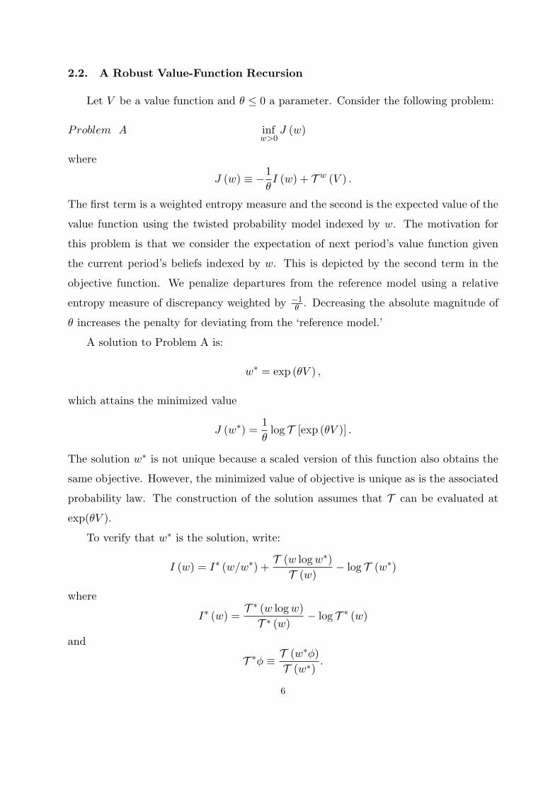
2.2. A Robust Value-Function Recursion
Let V be a value function and θ ≤ 0 a parameter. Consider the following problem:
Problem A infw>0
J (w)
where
J (w) ≡ −1
θI (w) + T w (V ) .
The first term is a weighted entropy measure and the second is the expected value of the
value function using the twisted probability model indexed by w. The motivation for
this problem is that we consider the expectation of next period’s value function given
the current period’s beliefs indexed by w. This is depicted by the second term in the
objective function. We penalize departures from the reference model using a relative
entropy measure of discrepancy weighted by −1θ . Decreasing the absolute magnitude of
θ increases the penalty for deviating from the ‘reference model.’
A solution to Problem A is:
w∗ = exp (θV ) ,
which attains the minimized value
J (w∗) =1
θlog T [exp (θV )] .
The solution w∗ is not unique because a scaled version of this function also obtains the
same objective. However, the minimized value of objective is unique as is the associated
probability law. The construction of the solution assumes that T can be evaluated at
exp(θV ).
To verify that w∗ is the solution, write:
I (w) = I∗ (w/w∗) +T (w logw∗)
T (w)− log T (w∗)
where
I∗ (w) =T ∗ (w logw)
T ∗ (w)− log T ∗ (w)
and
T ∗φ ≡ T (w∗φ)
T (w∗).
6

Notice that I∗ is itself interpretable as a measure of relative entropy and hence I∗(w/w∗) ≥0. Thus the criterion J satisfies the inequality:
4
J (w) = −1
θ
[
I∗ (w/w∗) +T (w logw∗)
T (w)− log T (w∗)
]
+ T w (V )
≥ −1
θ
[T (w logw∗)
T (w)− log T (w∗)
]
+ T w (V )
=1
θlog T [exp (θV )]
= J (w∗) .
Thus the solution to this entropy-penalized problem is a risk-sensitive adjustment to the
value function where
R (V ) =1
θlog{T [exp (θV )]}. (2.2)
2.3. A Larger Class of Perturbations
While formula (2.1) exploits the specific Markov structure of the candidate model,
the relative entropy measure has a straightforward extension to a much richer class of
perturbations. For instance, suppose that w is a strictly positive function that is allowed
to depend on both z and y. In this case we extend measure of entropy to be the following:
I (w) = E
[
w (z, y)
E [w (z, y) |y] log(
w (z, y)
E [w (z, y) |y]
)]
.
The solution to this extended version of Problem A remains the same. In other words, it
suffices for the ‘control’ w to depend only on the state tomorrow. Notice the perturbation
just described preserves the first-order Markov structure. That is, the ‘twisted’ process
remains a first-order Markov process.
First-order Markov perturbations are no doubt special. So it is of interest to extend
the class of perturbations further. We construct a bigger class of perturbations by
starting with positive (and appropriately measurable) functions that depend on the entire
past history of the Markov state for the reference process. Let t+ 1 denote tomorrow’s
date. Form the Radon-Nikodym derivative as:
ht+1 =w (zt+1, zt, zt−1, ...)
E [w (zt+1, zt, zt−1, ...) |zt, zt−1, ...].
4This proof mimics the proof of Proposition 1.4.2 in Dupuis and Ellis (1997), but is included for
completeness.
7

In other words, the time t + 1 Radon-Nikodym derivative is a strictly positive random
variable that is measurable with respect to the current and past values of the Markov
state (for the reference process). This random variable is constrained to have mean one
conditioned on zt, zt−1, .... The time t conditional entropy is then:
It (ht+1) = E [ht+1 log ht+1|zt, zt−1, ...]
and the time t counterpart to the objective function J for Problem A is:
Jt (ht+1) = −1
θIt (ht+1) + E [ht+1V (zt+1) |zt, zt−1, ...] .
Given that the process {zt} is Markov under the reference model, the solution to the
counterpart to the control problem A is to let the ‘control’ ht+1 be a function of the
Markov state zt+1 alone. Thus our solution to Problem A extends to this richer class
of perturbations, including ones for which the time t + 1 distortion fails to preserve
the Markov structure. The essential feature of these perturbations is that the transition
probability distribution for the candidate model be absolutely continuous with respect to
the transition probabilities of the reference model; this manifests itself in the restriction
that ht+1 > 0. Absolute continuity makes the log likelihood ratio criterion well defined.
3. Misspecification in Continuous Time
We now study the continuous-time counterpart to Problem A. As we will see subse-
quently, the continuous-time formulation can simplify the analysis. For instance, we will
show that when the reference model is a diffusion, a specification of w just introduces a
nonzero drift specification into Brownian motion increments that drive the model. Spe-
cific versions of Markov jump processes and mixed jump diffusion models can also be
handled. In the case of a Markov jump process, the misspecification w alters both the
jump intensities and the chain probabilities that dictate jump locations when a jump
takes place.
The operator formulation of continuous-time Markov processes entails specifying an
infinitesimal generator A. The conditional expectations are then given heuristically by:
Ts = exp (sA) .
8

This construction is formalized using a Yosida approximation. The domains of the
conditional expectation operators Ts will contain at least the space C of continuous
functions φ with limit zero as |x| → ∞; these are equipped with the sup norm. The
family or semigroup of conditional expectation operators {Ts ≥ 0} is assumed to be a
Feller semigroup, which among other things implies that
lims↓0
Ts = I
where I denotes the identity operator. (See Ethier and Kurtz, 1986, Chapter 1, for a
general discussion of semigroups and Chapter 4 for a discussion of Feller semigroups.)
3.1. Examples
When the reference model is a diffusion, the generator is a second-order differential
operator:
Aφ = µ · ∂φ∂x
+1
2trace
(
Σ ∂2φ∂x∂x′
)
,
where the coefficient vector µ is the drift of the diffusion and the coefficient matrix Σ is
the diffusion coefficient. The corresponding stochastic differential equation is:
dxt = µ (xt) dt+Σ1/2 (xt) dBt
where {Bt} is a multivariate standard Brownian motion. In this case the generator is not
a bounded operator and its domain excludes some of the functions in C. Nevertheless,
the generator’s domain includes at least functions that are twice differentiable and have
compact support. We have reason to extend this domain in our later analysis.
When the reference model is a Markov jump process, the generator can be represented
as:
Aφ = λ [Sφ− φ]
where the coefficient λ is a Poisson intensity parameter that dictates the jump probabili-
ties and S is a conditional expectation operator that encodes the transition probabilities
conditioned on a jump taking place. The intensity parameter can depend on the Markov
state and is bounded and nonnegative. In this case the domain of both the generator
and the semigroup can be extended to the space of bounded Borel measurable functions,
9
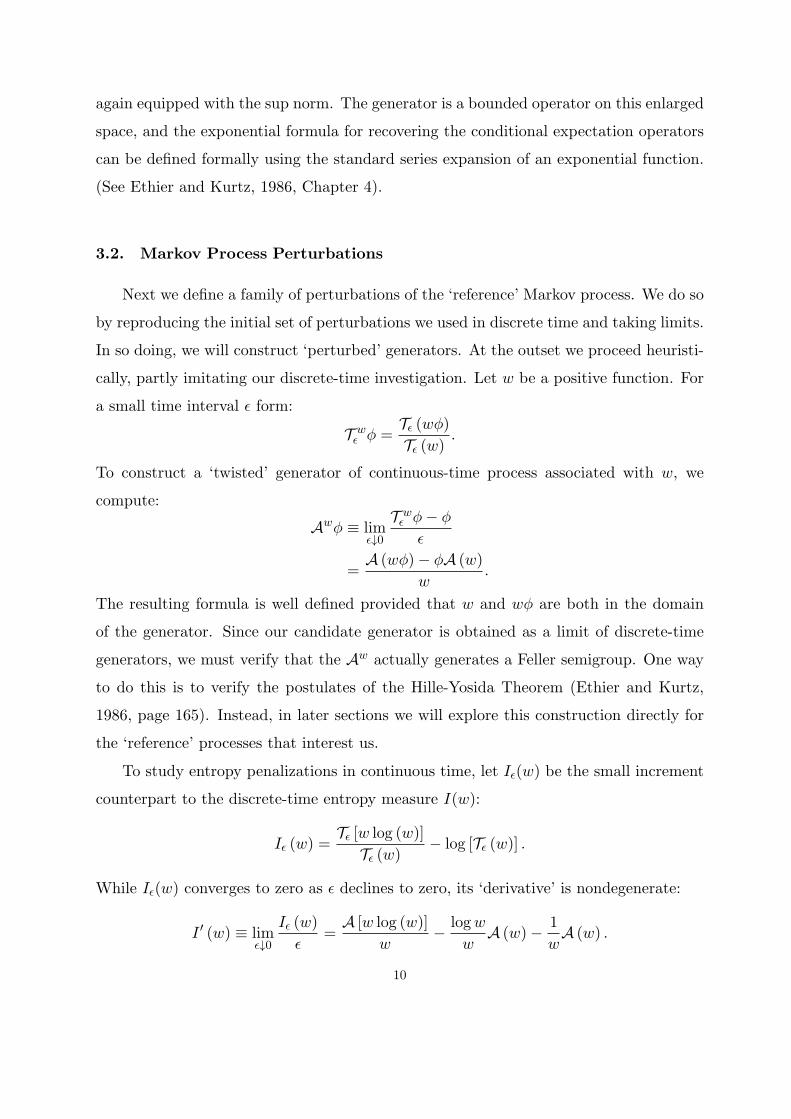
again equipped with the sup norm. The generator is a bounded operator on this enlarged
space, and the exponential formula for recovering the conditional expectation operators
can be defined formally using the standard series expansion of an exponential function.
(See Ethier and Kurtz, 1986, Chapter 4).
3.2. Markov Process Perturbations
Next we define a family of perturbations of the ‘reference’ Markov process. We do so
by reproducing the initial set of perturbations we used in discrete time and taking limits.
In so doing, we will construct ‘perturbed’ generators. At the outset we proceed heuristi-
cally, partly imitating our discrete-time investigation. Let w be a positive function. For
a small time interval ǫ form:
T wǫ φ =
Tǫ (wφ)Tǫ (w)
.
To construct a ‘twisted’ generator of continuous-time process associated with w, we
compute:
Awφ ≡ limǫ↓0
T wǫ φ− φ
ǫ
=A (wφ)− φA (w)
w.
The resulting formula is well defined provided that w and wφ are both in the domain
of the generator. Since our candidate generator is obtained as a limit of discrete-time
generators, we must verify that the Aw actually generates a Feller semigroup. One way
to do this is to verify the postulates of the Hille-Yosida Theorem (Ethier and Kurtz,
1986, page 165). Instead, in later sections we will explore this construction directly for
the ‘reference’ processes that interest us.
To study entropy penalizations in continuous time, let Iǫ(w) be the small increment
counterpart to the discrete-time entropy measure I(w):
Iǫ (w) =Tǫ [w log (w)]
Tǫ (w)− log [Tǫ (w)] .
While Iǫ(w) converges to zero as ǫ declines to zero, its ‘derivative’ is nondegenerate:
I ′ (w) ≡ limǫ↓0
Iǫ (w)
ǫ=
A [w log (w)]
w− logw
wA (w)− 1
wA (w) .
10

Since Iǫ(w) is nonnegative, so is I ′(w) ≥ 0, and I ′(w) equals zero when w is constant.
Combining these two limiting operators, we can construct a continuous-time coun-
terpart to criterion J :
J ′ (w) = −1
θI ′ (w) +AwV.
Thus to perform a robust version of continuous-time value function updating we are led
to solve:
Problem B infw>0,w∈D
J ′ (w)
where D is constructed so that both w and wV are in the domain of the generator.5
As in discrete time, we will verify that
w∗ = exp (θV )
solves Problem B. The resulting optimized value of the criterion is:
J ′ (w∗) =1
θ
A [exp (θV )]
exp (θV ).
To check the solution, we imitate the argument we gave for the discrete-time counterpart.
We start by changing the reference point for the relative entropy measure by using the
‘twisted’ generator A∗ = Aw with w = w∗ in place of A:
I∗′ (w) ≡ A∗ [w log (w)]
w− logw
wA∗ (w)− 1
wA∗ (w) .
It may be verified that
I∗′ (w/w∗) = I ′ (w)− I ′ (w∗)− θAw (V ) + θA∗ (V )
= −1
θ
[
J ′ (w)− J ′ (w∗)]
.
Since the left-hand side is always nonnegative and θ is negative, it follows that w∗ solves
Problem B.
5Given the presence of the inf instead of a min the restrictions on w are not problematic. However,
restricting V to be in the domain of generator is sometimes too severe. This restriction can be relaxed byinstead using the extended generator.
11

3.3. Risk-Sensitive Recursion
In this subsection, we deduce the continuous-time counterpart to the risk sensitive
recursion (2.2). This allows us to find a link in continuous time between entropy-based
robustness and recursive utility theory as formulated by Duffie and Epstein (1992). The
small interval counterpart to operator R given in (2.2) is
RǫV ≡ 1
θlog Tǫ [exp (θV )] .
As ǫ declines to zero, this operator collapses to the identity operator. Our interest is in
the derivative (with respect to ǫ) of this operator (evaluate at ǫ = 0):
limǫ↓0
RǫV − V
ǫ=
1
θ
A [exp (θV )]
exp (θV )
= J ′ (w∗) .
We will have more to say about this connection between entropy and risk sensitivity
after we add specificity to the continuous-time processes.
3.4. A Robust Value Function Recursion
We now revisit the question we posed out the outset of section two. In discrete
time, the usual fixed point problem for evaluating a time-invariant control law under
discounting and an infinite horizon is:
V (x) = ǫU (x) + exp (−ǫδ) TǫV (x)
where U is the current-period reward function and δ is the subjective rate of time dis-
count. We obtain continuous-time counterpart by subtracting V from both sides, divid-
ing by ǫ, and taking limits. This results in:
0 = U − δV +AV.
When we introduce adjustments for model misspecification, we modify this to be
0 = U − δV +1
θ
A [exp (θV )]
exp (θV ),
which can be viewed as one of the utility recursions studied by Duffie and Epstein (1992).
12

The connection between risk sensitivity and robustness is familiar from the literature
on risk-sensitive control (e.g. see James (1992) and Runolfsson (1994)). In contrast
to that work, we consider control problems with discounting, which leads to study a
recursive formulations of risk sensitivity. The resulting recursion is the continuous-time
generalization of one studied by Hansen and Sargent (1995).6
4. Continuous-Time Diffusions
In this section we study the solution to Problem B when the underlying reference
model is a diffusion. We then describe a larger class of perturbations in continuous-time
that are consistent with our entropy-based notion of robustness.
4.1. Markov Perturbations
We start by revisiting the class of perturbations that we studied earlier, but special-
ized to the diffusion model. Hence, we take the generator to be:
Aφ = µ · ∂φ∂x
+1
2trace
(
Σ ∂2φ∂x∂x′
)
,
and, as before, we consider a twisted generator:
Awφ =A (wφ)− φA (w)
w.
Note that by the product rule for first and second derivatives:
A (wφ) = wAφ+ φAw +
(
∂w
∂x
)′
Σ
(
∂φ
∂x
)
.
Thus the twisted generator can be depicted by:
Awφ = Aφ+ u′Σ1/2
(
∂φ
∂x
)
where we have defined u to be:
u ≡ Σ1/2∂ logw
∂x.
6The discrete-time recursion is the same as that used by Weil (1993), although Weil does not demon-
strate the connection to risk-sensitive control theory.
13
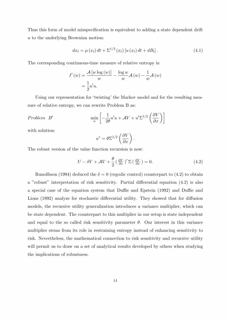
Thus this form of model misspecification is equivalent to adding a state dependent drift
u to the underlying Brownian motion:
dxt = µ (xt) dt+Σ1/2 (xt) [u (xt) dt+ dBt] . (4.1)
The corresponding continuous-time measure of relative entropy is:
I ′ (w) =A [w log (w)]
w− logw
wA (w)− 1
wA (w)
=1
2u′u.
Using our representation for ‘twisting’ the Markov model and for the resulting mea-
sure of relative entropy, we can rewrite Problem B as:
Problem B′ minu
[
− 1
2θu′u+AV + u′Σ1/2
(
∂V
∂x
)]
with solution:
u∗ = θΣ1/2
(
∂V
∂x
)
.
The robust version of the value function recursion is now:
U − δV +AV +θ
2( ∂V∂x )′Σ( ∂V
∂x ) = 0. (4.2)
Runolfsson (1994) deduced the δ = 0 (ergodic control) counterpart to (4.2) to obtain
a ”robust” interpretation of risk sensitivity. Partial differential equation (4.2) is also
a special case of the equation system that Duffie and Epstein (1992) and Duffie and
Lions (1992) analyze for stochastic differential utility. They showed that for diffusion
models, the recursive utility generalization introduces a variance multiplier, which can
be state dependent. The counterpart to this multiplier in our setup is state independent
and equal to the so called risk sensitivity parameter θ. Our interest in this variance
multiplier stems from its role in restraining entropy instead of enhancing sensitivity to
risk. Nevertheless, the mathematical connection to risk sensitivity and recursive utility
will permit us to draw on a set of analytical results developed by others when studying
the implications of robustness.
14

4.2. Enlarging the Class of Perturbations
The robust discounted value function recursion (4.2) can be obtained in a somewhat
different manner. This alternative formulation will permit us to expand the class of
twisted models that we can consider. Following James (1992), we alter the time t reward
function of the decision maker by augmenting U(xt) with − 12θ |gt|2. The objective of the
robust decision-maker has a nonrecursive representation:∫ ∞
0exp (−δt)
[
U (xt)−1
2θ|gt|2
]
dt, (4.3)
and the state evolution is:
dxt = µ (xt) dt+Σ1/2 (xt) [gtdt+ dBt] . (4.4)
The ‘control’ vector process {gt} is suitably adapted to the filtration generated by the
underlying Brownian motion vector. It has the interpretation of distorting the Brownian
by appending a state dependent drift to it. The magnitude of this distortion is restrained
by the relative entropy penalty − 12θ |gt|2. As θ converges to zero, it becomes optimal to
set g to zero.
Given the Markov structure, the solution to this control problem can be represented
as a time-invariant function of the state vector xt, which we denote: gt = u(xt). Notice
that (4.1) and (4.4) coincide when under a time invariant control law. The resulting
Bellman equation is identical to (4.2), and hence the optimal ‘control’ satisfies:
gt = θΣ1/2
(
∂V
∂x
)
(xt) .
We can now think of (1/2)|gt|2 as a time t measure of relative entropy but for a more
general family of perturbations. Now a perturbation in the reference diffusion process is
obtained by introducing a (progressively measurable) process {gt} and appending a drift∫ to gsds to the Brownian motion Wt. This form of perturbation admittedly still looks
very special. From our discussion of discrete-time models we are led to expect a large
class of perturbations with finite (relative entropy). However, from Girsanov’s Theorem,
it is evident that there is little scope for further enlargements. Absolute continuity is
a potent restriction for continuous-time diffusions.7
Also, even these seemingly simple
drift distortions still result in a rather rich collection of candidate models.7See, e.g., Karatzas and Shreve (1991, pages 190-196), Durrett, (1996, pages 90-93) and Dupuis and
Ellis (1997, pages 123-125).
15
4.3. Adding Controls to the Original State Equation
We now add a control vector to the original state evolution equation:
dxt = µ (xt, it) dt+Σ1/2 (xt, it) (gtd t+ dBt) (4.5)
and to the return function: U(x, i) where it is a control vector. Consider a time-invariant
control of the form it = f(xt). The value function for the risk-sensitive (or the robust)
control problem satisfies (4.2), except that now the differential operatorA and the reward
function U depend on the control law f :
U (·, f)− δV +A (f)V +θ
2( ∂V∂x )′Σ(·, f) ( ∂V
∂x ) = 0.
As we have seen, for a fixed control law f , this equation can emerge from solving a single
agent ‘robust control problem.’ Thus we can solve for the optimal (or robust) control
law by solving a two-player Markov game:
maxf
minu
[
U (x, f)− δV (x) +A (f)V (x) + ( ∂V∂x (x) )′Σ1/2 (x, f)u− 1
2θu′u
]
.
5. Market Price of Risk
In this section, we study the continuous-time analog to the (shadow) market price
of risk. This permits us to study how the market price of risk is enhanced by a concern
about robustness. That is, we show us how risk aversion as reflected in security prices can
be reinterpreted in part as depicting an aversion to model misspecification or Knightian
uncertainty. The result will be a formula analogous to one obtained by Hansen, Sargent
and Tallarini (1997) as an approximation in discrete time.
We derive this formula by computing shadow prices for a fictitious social planner.
Let {Pt} denote a valuation process for an asset that is held over a small increment of
time and has no dividend payouts during that interval. (Alternatively, we can think
of the dividends as being reinvested). Let {Mt} be a process used to depict the im-
plied stochastic discount factors. This process is constructed to satisfy the discrete-time
pricing relation:
16

exp (−sδ)Et{exp [θV (xt+s)]Pt+sMt+s} = Et{exp [θV (xt+s)]}MtPt (5.1)
for all increments s, where Et is the time t conditional expectation operator associated
with the underlying Brownian motion. Thus the stochastic discount factor between time
periods t and t+ s is given by the ratio exp(−sδ)Mt+s/Mt.
For convenience, we have defined stochastic discount factors in order that assets
are valued in accordance to the twisted Markov process where the ‘twisting’ coincides
that obtained as the solution to the optimal resource allocation problem. The Radon-
Nikodym derivative used to depict this twisting:
exp [θV (xt+s)]
Et{exp [θV (xt+s)]}
which agrees with our earlier analysis of robustness in decision making. By using the
twisted probability measure, the process {Mt} is directly interpretable as the marginal
utility process for the consumption numeraire. Consequently, what we refer to as a
stochastic discount factor is also an intertemporal marginal rate of substitution. The
twisting of the probability is induced by the preference for robustness, and our aim is to
characterize its contribution to the market price of risk.8
For the Markov economies we study, the process {Mt} is representable asMt = Φ(xt).
For instance, this occurs when there is a single consumption good that is chosen optimally
by the social planner to be a time invariant function of the Markov state. Express the
local evolution as
dMt =Mtµm,tdt+Mtσm,t · dBt
where:
µm,t =∂ log Φ
∂x
′
(xt)µ∗ (xt) +
1
2Mttrace
(
Σ∗ ∂2Φ∂x∂x
)
(xt) ,
and
σm,t =∂ log Φ
∂x
′
(xt) [Σ∗ (xt)]
1/2 .
8The decomposition we deduce is a bit misleading because a preference for robustness can result in
changing the consumption-investment profile and hence have a direct effect on the stochastic discountfactor. Instead we are focusing on an additional increment in the market price of risk that will be presenteven when the equilibrium consumption process is unaltered.
17

In these formulas µ∗(x) is the drift coefficient for the Markov process {xt} when the
optimal, time-invariant control law for it is imposed. Similarly, Σ∗ is the diffusion matrix
associated with the solution to the optimal resource allocation problem.
Suppose the valuation process satisfies:
dPt = Ptµr,tdt+ Ptσr,t · dBt.
We refer to µr,t as the time t instantaneous mean rate of return and (σr,t · σr,t)1/2 as
the corresponding instantaneous standard deviation. In what follows, we will think of
modeling an instantaneous return by specifying the pair (µr,t, σr,t). Equilibrium asset
pricing imposes explicit restrictions on this pair, and the instantaneous market price of
risk shows depicts the equilibrium trade-off between (local) mean rates of return and the
corresponding standard deviations.
As is standard when investigating asset pricing models, we deduce the restrictions
on the local mean of an asset return, µr,t given the ‘loading’ vector σr,t on the Brownian
motion ‘factors’. Thus, we derive the risk prices for the Brownian increments, and then
we assimilate these prices to form the market price of risk. Since pricing relation (5.1)
holds for all s, we find that:
−δ + µm,t + µr,t + σr,tσ′m,t + θ (σr,t + σm,t) [Σ
∗ (xt)]1/2 ( ∂V
∂x ) (xt) = 0.
This relation is the continuous-time counterpart to the familiar consumption Euler equa-
tion. From this relation, it follows that the risk free rate is obtained by setting σr,t to
zero:
rf,t = δ − µm,t − σm,t · g∗t (5.2)
where u∗t is robust adjustment to the Brownian motion at date t. Thus we may rewrite
the instantaneous pricing relation as:
µr,t − rf,t = −σr,t · (σm,t + g∗t ) . (5.3)
Thus the ‘risk prices’ for the Brownian increments are given by the entries of the vector
−σm,t − g∗t . The first term is familiar from the usual investigation of the consumption
capital asset pricing model (e.g., Breeden, 1979). The second component −g∗t is an
added premium that is induced by the concern for model misspecification.
18

The market price of risk is the slope of the mean-standard frontier for the full array
of asset returns. Applying the Cauchy-Schwarz inequality to (5.3), it follows directly
(5.3) that:
|µr,t − rf,t| ≤ (σr,t · σr,t)1/2 [(σm,t + g∗t ) · (σm,t + g∗t )]1/2
Consequently, the market price of risk is:
mprt =[(
σm,t + g∗′t)
· (σm,t + g∗t )]1/2
. (5.4)
This formula extends an approximation result that Hansen, Sargent and Tallarini (1997)
derived for discrete-time economies.9
Formulas (5.2) and (5.4) show how a concern for model misspecification alters market-
based measures of risk premia.
6. A Robust Precautionary Motive
Hansen, Sargent and Tallarini (1997) obtained a robust interpretation of the ratio-
nal expectations version of the permanent income model of consumption. Under this
robustness interpretation, consumers in effect are endowed with a precautionary motive
for saving as a device to guard against a family of model misspecifications. In this sec-
tion, we use a discounted version of a value function expansion due to James (1992) to
show that the ”robust” mechanism for precautionary behavior carries over to a richer
class of control problems. We are also able to distinguish the impact of robustness from
the more familiar precautionary motive described by Leland (1968), Kimball (1990) and
others. In addition, it permits to reinterpret the precautionary motive investigated by
Weil (1993).
The value function expansion of James (1992) relies on a small noise expansion.
Instead of investigating a single optimal resource allocation problem, we study a family
9Hansen, Sargent and Tallarini (1997) studied permanent income-type economies in which the risk-free
rate is pinned down by the specification of the technology. They adjusted the subjective discount factorto compensate for the impact of formula (5.2) in equilibrium.
19
of problems indexed by the magnitude of the risk. We replace the original evolution
equation with:
dxt = µ (xt, it) dt+√ǫΣ1/2 (xt, it) dBt
where ǫ indexes the magnitude of the risk. Associated with this family of evolution
equations is a family of generators: Aǫ(i). As in (4.5), the ‘robust’ counterpart to this
family of evolution equations is:
dxt = µ (xt, it) dt+√ǫΣ1/2 (xt, it) (gt + dBt) .
Finally, the value functions for the corresponding two-player games satisfy the partial
differential equation:
U (·, i)− δVǫ +Aǫ (i)V + ǫθ
2( ∂Vǫ
∂x )′Σ(·, i) ( ∂Vǫ∂x ) = 0.
To obtain a value function expansion, we differentiate this partial differential equa-
tion with respect to ǫ and evaluate it at ǫ = 0. Of course, the decision rule for the control
it will also depend on ǫ. Since the control is chosen optimally, this dependence does not
alter the first-order (in ǫ) expansion of the value function. Instead we are free to ignore
this dependence when differentiating with respect to ǫ.
To obtain a path about which to approximate, we solve the deterministic differential
equation:
dx0t = µ(
x0t , i0t
)
dt
given an initial condition x0 = x where i0t is the time t optimal control in the absence
of risk (ǫ = 0. Let DV denote the derivative of the value function with respect to ǫ
evaluated at ǫ = 0. Then this derivative (assuming it exists) satisfies the recursion:
−δDV + µ · ( ∂DV∂x ) +Wn + θWr = 0 (6.1)
where
Wn ≡ 1
2trace
(
Σ0 ∂2V0∂x∂x′
)
,
Wr ≡1
2
(
∂V0∂x
)′Σ0
(
∂V0∂x
)
,
and Σ0 is the diffusion matrix when computed at x0t , i0t .
20
Notice that (6.1) is a first-order partial differential equation in DV . Its solution may
be depicted as follows. Solve the (deterministic) differential equation:
dx0t = µ(
x0t , i0t
)
dt
given an initial condition x0 = x where i0t is the optimal control in the absence of
uncertainty. Then
DV (x) =
∫ ∞
0exp (−δt)
[
Wn
(
x0t)
+ θWr
(
x0t)]
dt.
Thus we are led to the following value-function expansion:
V (x) ≈ V0 (x) + ǫDV (x)
This expansion is just the discounted counterpart to the one given in Theorem 5.1 of
James (1992).
Robustness shows up in this value function expansion through the term θWr, and
increasing θ in magnitude enhances the contribution of this term. In the absence of
robustness (θ = 0) we obtain the familiar contribution Wn. Notice that while Wn
depends on the second derivative of the value function from the deterministic control
problem, Wr is constructed from the first derivative of this value function. Thus the
precautionary motive introduced by robustness has a rather different character than that
obtained in the absence of robustness. Moreover, for a given (small) amount of ‘risk’
(a given ǫ), θ∫∞
0 exp(−δt)Wr(x0t )dt measures how much utility loss can be attributed
to the robustness motive. It may be used as a device for interpreting the robustness
parameter ‘theta.’
21

7. An Alternative Formulation of Robustness
In our treatment of entropy-based robustness, we have used penalization indexed
by the so-called risk sensitivity parameter θ. Suppose that we now alter the problem to
mimic instead a recursive formulation of Knightian uncertainty, following in part Epstein
and Wang (1994). Instead of penalizing entropy, we constrain each period (instant). In
continuous time Markov formulation, we impose the constraint:
I ′ (w) ≤ η.
In what follows, we focus on the special case of a diffusion. Thus we require that the
drift distortion satisfy:1
2|gt|2 ≤ η.
We find a ‘robust’ control law by guarding against the worst case appropriately con-
strained. Again the ‘solution’ for gt is a time invariant function of the Markov state, so
that g∗t = u∗(xt) for some function u∗.
The function u∗ should solve:
minu
[
U − δV +AV + u′Σ1/2
(
∂V
∂x
)]
subject to1
2u′u = η.
The solution to this problem is:
u∗ = −√
2ηΣ1/2
(
∂V∂x
)
[
(
∂V∂x
)′Σ(
∂V∂x
)
]1/2.
Thus the robust version of value function updating now entails solving:
U − δV +AV −√
2η
[
(
∂V
∂x
)′
Σ
(
∂V
∂x
)
]1/2
= 0
In the small-noise expansions of the penalized ”robust control” problem, robustness
imitates second-order risk aversion. This is evident because the first term to enter is
22
a variance, not a standard deviation. In the small noise expansion for this alternative
‘constrained’ robustness the first term to enter will be the standard deviation.10
8. Multiple Agents
In this section we consider an extension of the model by introducing heterogeneous
agents. Our reason for doing so is that familiar efficient allocation rules cease to apply
in this framework. Even under optimal resource allocation, individual agents will not be
allocated a time-invariant function of the aggregate ‘pie.’ Instead histories will matter,
but in a very particular way. As a consequence, even when allocations are Pareto optimal,
multiple agent models can look quite different from single-agent counterparts. Given the
close connection between our model of robustness and recursive utility theory, we are
able to exploit recent work by Dumas, Uppal and Wang (1997) for justification.
For simplicity, we consider an endowment economy with a single consumption good.
The aggregate endowment is given by:
ca = g (x)
which is to be allocated across consumers. Abusing notation, we let U denote the
common period utility function with arguement cj for person j. Thus we have the
resource constraint:n∑
j=1
cj = g (8.1)
We follow Negishi (1960), Lucas and Stokey (1984), Epstein (1987) and others by using
Pareto factors to construct a social welfare function used to allocate consumption among
the individual consumers. This function will be constructed so that the intertemporal
marginal rates of substitution are equated. Asset prices are then built from the common
marginal rates of substitution.
10This difference shows up because in the latter case the ‘multiplier’ on specification error constraint
will shrink to zero when the noise covariance diminishes to zero. On the other hand, we previously heldfixed the penalty parameter, which we may think of as being analogous to a multiplier on a specification-error constraint. When taking small noise expansions, it is not clear that the penalty parameter θ shouldbe held fixed, nor is it clear that η should be held fixed.
23

Dumas, Uppal and Wang (1997) show that efficient allocations may be found by
deducing a social welfare function that depends on an endogenous state vector of Pareto
factors λt for each t. Each component of the Pareto factor vector is matched to an
indivual (or individual type) in the economy. Thus the time t Pareto factor for person
j is denoted λjt . The social welfare function S depends both on the exogenous state
vector x and the endogenous state vector λ. This function is a homogeneous of degree
one function that satisfies the partial differential equation:
0 = maxc
n∑
j=1
λj[
(
θSj + 1)
U(
cj)
− δ
θ
(
θSj + 1)
log(
θSj + 1)
+ASj
]
(8.2)
subject to (8.1) where the U notation is now used to the common instanteous utility
function for each consumer and Sj is:
Sj (x, λ) =∂S (x, λ)
∂λj.
We continue to use the A notation to depict the local evolution of {xt} (but not of the
Pareto factor vector process {λt}):
ASj =∂Sj (x, λ)
∂x· µ (x) + 1
2trace
(
Σ∂2Sj (x, λ)
∂x∂x′
)
.
From the social welfare function W , we may construct the entropy-adjusted value
functions for each individual via:
V j =log
(
θSj + 1)
θ.
Moreover, the evolution of the Pareto factors is given by:
dλjt = −λjt(
δ − θ[
U j (x, λ)− δV j (x, λ)])
dt
where U j is the function U evaluated at the efficient choice of cj given as a function of
the state vectors x and λ. Notice that the Pareto factors are locally predictable. We let
γ denote the composite drift term obtained by stacking the individual drifts.11
11When U is log, it can be shown that the solution to (8.2) implies that the drift for λj is −δ for
every consumer and that V j = V a + dj where the function V a is common to all consumers and dj
is constant (across states). Thus the Pareto factors ρj share a common constant drift and a commonweighted Brownian motion increment. In this log case, standard representative consumer aggregationresults apply: individual consumptions are proportional to aggregate consumption with a time and stateinvariant proportionality factor. See Tallarini (1997) for a quantitative investigation of a single consumerlog specification using the ‘risk-sensitive’ utility recursion.
24

To characterize the alloation rule, we introduce a multiplier κ on the resource con-
straint (8.1). The first-order conditions imply that
ρjU ′(
cj)
= κ
where
ρj ≡ λj exp(
θV j)
.
Thus the allocations satisfy:
cj =(
U ′)−1
(
κ
ρj
)
where κ is determined by (8.1).
In the appendix we show formally how to obtain these formulas from Dumas, Uppal
and Wang (1997). By construction, the individual value funtions satisfy the entropy-
adjusted partial differential equation:
U j − δV j +AV j + γ · ∂Vj
∂λ+θ
2
(
∂V j
∂x
)′
Σ
(
∂V j
∂x
)
= 0 (8.3)
for j = 1, 2, ..., n.
25

A. Two Equivalent Ways to Represent Preferences
In this appendix, we deduce two alternative ways to depict prefences for diffusion
models. One uses the transformation suggested by Duffie and Epstein (1992) and Duffie
and Lions (1992). The other one uses a transformation suggested by Dumas, Uppal and
Wang (1997) used to depict the preferences has having endogenous discounting instead
of robustness. We consider intially a single-agent formulation, and then we study the
multiple-agent counterpart.
A.1. An Expected-value Recursion
Recall the value-function updating recursion under robustness:
U ◦ g − δV +AV +θ
2
(
∂V
∂x
)′
Σ
(
∂V
∂x
)
= 0 (A.1)
where we evaluate the current-period utility function at
c = g (x)
This equation is nonlinear in the partial derivatives of the value function V . Following
Duffie and Epstein (1992) and Duffie and Lions (1992), we now transform this equation
into one that is linear the partial derivatives but nonlinear in the value function. We
accomplish this by taking an increasing transformation of V :
S =exp (θV )− 1
θ.
Hence S is a monotone transformation of the original value function, and it has a well
defined limit when θ = 0 (S = V ). Inverting this relation, we have
V =log (θS + 1)
θ.
Moreover,
exp (θV ) = θS + 1
Multiply (A.1) by exp(θV ), and we see that
(θS + 1)U ◦ g − δ
θ(θS + 1) log (θS + 1) +AS = 0. (A.2)
26

Note that while this partial differential equation is nonlinear in S, it is linear in the
derivatives of S. Duffie and Epstein (1992) depict a corresponding expected value recur-
sion associated with the partial differential equation system.
A.2. Endogenous Discounting
We deduce a third depiction of the recursion, which is the continuous-time counter-
part to the variational utility recursion of Geoffard (1996). This representation has an en-
dogenous discount rate bt at date t and a corresponding discount factor exp(−∫ s0 bt+u)du
between date t and date t+ s. Eventually, we will introduce a different discount factor
process for each consumer, and these discount factors will be relabeled as Pareto factors.
To deduce the discount factor representation of preferences, we follow Dumas, Uppal
and Wang (1997) by computing the Legendre transform:
U∗ (b, c) = maxS
[
(θS + 1)U (c)− δ
θ(θS + 1) log (θS + 1) + bS
]
where S is a stand in for the value and b is the stand in for the discount rate. Use the
change of variables:
S∗ = θS + 1.
Then an equivalent problem to the Legendre transform is:
U∗ (b, c) = minS∗
[
S∗U (c)− δ
θS∗ log (S∗) +
b
θ(S∗ − 1)
]
.
The first-order conditions are:
U (c)− δ − b
θ− δ
θlog (S∗) = 0.
Thus
log (S∗) =θ
δU (c)− δ − b
δ,
and
U∗ (b, c) = − bθ+δ
θS∗
= − bθ+δ
θexp
[
θU (c)− δ + b
δ
]
.
27

Consistent with our discount rate interpretation, we introduce an endogenous state
variable λt with dynamic evolution:
dλt = −btλtdt,
We depict preferences by having consumers choose a discount rate process {bt} to mini-
mize:
E0
[∫ ∞
0λtU
∗ (bt, ct)
]
.
Given time invariant Markov dynamics for the optimal resource allocation problem,
with consumption being a time invariant function of xt, the minimization problem is
Markovian with a time-invariant control law for the discount rate process. Notice that
the discount factor process is taken to be locally predictable.
The value function for this problem is given by λS(x) where S solves (A.2). Moreover,
the first-order conditions for the discount rate process are obtained by solving:
minbU∗ (b, c)− bS.
Hence b should solve:
−1
θ+
1
θexp
[
θU (c)− δ + b
δ
]
− S = 0.
Therefore,
θU (c)− δ + b = δ log (θS + 1) ,
or
b = δ − θ [U (c)− δV (x)] .
The ‘endogenous’ discount factor rate is pulled away from δ depending on how close the
period utility function is to the entropy adjusted (and discounted) value function.
28

A.3. A Multiple-Agent Counterpart
As argued by Dumas, Uppal, and Wang (1997), the single-agent discount factor
representation may be used to construct to a multiple agent counterpart in which the
discount factor processes of each agent play the role of Pareto factors in an optimal
resource allocation problem. Thus we now introduce a Pareto factor process for each
person, with evolution given by:
dλjt = −bjtλjtdt
for j = 1, 2, ..., n. We stack the date t λ’s into a composite (n-dimensional) state vector
λt with (degenerate) Markov dynamics.
For simplicity, we consider an endowment economy in which aggregate consumption
is a time invariant function of the Markov state xt:
n∑
j=1
cj = g (x) . (A.3)
We use the Pareto weight processes to split aggregate consumption across agents. When
these processes are proportional, the allocation rules are time-invariant functions of
the Markov state. This will be true in the limiting case in which θ is set to zero (no
relative entropy adjustments.) More generally, the efficient allocation rules are history
dependent, and the λ processes are convenient ways to keep track of this dependence.
We solve the multiple-agent optimal resource allocation problem by computing a
social welfare function S that depends on the vector of Pareto factors. This function will
be homogeneous of degree one in the vector vector, and individual utilities at each date
can be deduced using Euler’s decomposition of a homogeneous of degree one function:
W (x, λ) =
n∑
j=1
λjSj (x, λ)
where
Sj (x, λ) ≡ ∂S (x, λ)
∂λj.
Analogous to our single-agent model, we may view λjSj(x, λ) as the value function for
person j.
29

We produce a functional equation for the social value function S. This function
depends on both the λ vector of Pareto weights and the original Markov state vector x.
When there are multiple consumers, we are led to solve:
0 = maxc
minb
n∑
j=1
λj[
U∗(
cj , bj)
− bjSj (x, λ) +ASj (x, λ)]
subject to the resource constraint
n∑
j=1
cj = g (x) .
The local operator A applied to Sj uses derivatives with respect to x, but not λ.
To solve the minimization component of this two-player game, we construct the
entropy-adjusted counterpart to be:
V j ≡ exp(
θSj)
− 1
θ.
Then the discount rates for the Pareto factors satisfy:
bj = δ − θ[
U(
cj)
− δV j (x, λ)]
(A.4)
for the optimal allocation of consumption across people. Thus the decision about the
Pareto factor adjustment is based on a comparison of the current period utility and the
current period entropy-adjusted values.
Given the solution for the discount rates (A.4), it can be shown that
exp
[
θU(
cj)
− δ + bj
δ
]
= exp(
θV j)
.
Therefore, the Sj ’s also solve heterogeneous agent counterpart to to the Duffie-Lions
partial differential equation (A.1):
0 = maxc
n∑
j=1
λj[
(
θSj + 1)
U(
cj)
− δ
θ
(
θW j + 1)
log(
θSj + 1)
+ASj
]
(A.5)
subject ton∑
j=1
cj = g.
30

References
Breeden, D. T. (1979), ”An Intertemporal Asset Pricing Model with Stochastic Con-sumption and Investment Opportunities,” Journal of Financial Economics 7, 265-296.
Csiszar, I. (1991), ”Why Least Squares and Maximum Entropy? An Axiomatic approachto Inference for Linear Inverse Problems,” The Annals of Statistics 19:4, 2032-2066.
Dumas, B. Uppal, R. and T. Wang (1997), ”Efficient Intertemporal Allocations withRecursive Utility,” manuscript.
Durrett, R., (1996), Stochastic Calculus: A Practical Introduction, Boca Raton: CRCPress.
Duffie, D. and L.G. Epstein (1992), ”Stochastic Differential Utility,” Econometrica 60:2,353-394.
Duffie, D. and P.L. Lions (1992), ”PDE Solutions of Stochastic Differential Utility,”Journal of Mathematical Economics 21, 577-606.
Dupuis, P. and R. S. Ellis (1997), A Weak Convergence Approach to the Theory of Large
Deviations, New York: John Wiley and Sons.
Epstein, L.G. and T. Wang (1994), ”Intertemporal Asset Pricing Under Knightian Un-certainty,” Econometrica 62:3, 283-322.
Epstein, L.G. and S.E. Zin (1989), ”Substitution, Risk Aversion and the Temporal Be-havior of Consumption and Asset Returns: A Theoretical Framework,” Econometrica
57:4, 937-969.
Ethier, S.N. and T.G. Kurtz (1986), Markov Processes: Characterization and Conver-
gence, NY: John Wiley and Sons.
Fleming, W.H. and W.M. McEneaney (1995), ”Risk-Sensitive Control on an InfiniteTime Horizon,” SIAM Journal of Control and Optimization 33:6, 1881-1915.
Geoffard, P. Y. (1996), ”Discounting and Optimizing: Capital Accumulation as a Vari-ational Minmax Problem,” Journal of Economic Theory, 66, 53-70
Hansen, L.P. and T.J. Sargent (1995), ”Discounted Linear Exponential Quadratic Gaus-sian Control,” IEEE Transactions on Automatic Control 40:5, 968-971.
Hansen, L.P., T.J. Sargent and T.D. Tallarini, Jr. (1997), ”Robust Permanent Incomeand Pricing,” manuscript.
James, M.R. (1992), ”Asymptotic Analysis of Nonlinear Stochastic Risk-Sensitive Con-trol and Differential Games,” Mathematics of Control, Signals, and Systems 5, 401-417.
Karatzas, I. and S. E. Shreve (1991), Brownian Motion and Stochastic Calculus, SecondEdition, New York: Springer-Verlag.
Kimball, M. S. (1990), ”Precautionary Savings in the Small and in the Large,” Econo-
metrica 58, 53-73.
Lucas, R. and N. Stokey (1989), ”Optimal Growth with Many Consumers,” Journal of
Economic Theory, 32, 139-171.
Negishi, T. (1960), ”Welfare Economics and Existence of an Equilibrium for a Compet-itive Economy,” Metroeconomica, 12, 92-97
31

Runolfsson, T. (1994), ”The Equivalence between Infinite-horizon Optimal Control ofStochastic Systems with Exponential-of-integral Performance Index and Stochastic Dif-ferential Games,” IEEE Transactions on Automatic Control 39, 1551-1563.
Runolfsson, T. (1995), ”Risk-sensitive Control of Stochastic Hybrid Systems,” Proceed-
ings of the 34th Conference on Decision and Control, New Orleans, LA.
Shore, J.E. and R.W. Johnson (1980), ”Axiomatic Derivation of the Principle of Max-imum Entropy and the Principle of Minimum-Cross Entropy,” IEEE Transactions on
Information Theory 26:1, 26-37.
Weil, P. (1993), ”Precautionary Savings and the Permanent Income Hypothesis,” Review
of Economic Studies 60, 367-383.
32


