

i
Risk based structural design of double hull tankers
Joana Pires Guia
Thesis to obtain the Master Degree in
Naval Architecture and Marine Engineering
Supervisors: Doutor Ângelo Manuel Palos Teixeira, Doutor Carlos António Pancada
Guedes Soares
Examination Committee
Chairperson: Doutor Carlos António Pancada Guedes Soares
Supervisor: Doutor Ângelo Manuel Palos Teixeira
Members of the Committee: Doutor Bruno Constantino Beleza de Miranda Pereira
Gaspar
November 2014

ii

iii
Acknowledgements
My deepest gratitude to Professor Ângelo Palos Teixeira for his guidance, availability and shared
knowledge which helped improve the content of the present work.

iv

v
Resumo
O objetivo do presente trabalho é desenvolver uma abordagem baseada no risco para o projeto
estrutural de um petroleiro Suezmax. A concretização deste objetivo envolveu a avaliação da
resistência última do navio e do seu nível de fiabilidade estrutural, das consequências da falha da
estrutura primária do navio e do seu nível de segurança ótimo com base numa análise de custo-
benefício.
Os recentes desenvolvimentos das abordagens ao projeto estrutural de navios baseado no risco, bem
como o trabalho realizado pela IMO (International Maritime Organization) no desenvolvimento da
metodologias Avaliação Formal de Segurança (FSA – Formal Safety Assessment) e normas
baseadas em objetivos (GBS – Goal Based Standards) são revistos.
A formulação do problema de fiabilidade da estrutura do navio baseia-se na análise do colapso
progressivo (PCA – Progressive Collapse Analysis) proposta pela IACS (International Association of
Classification Societies) para obter a resistência última da secção mestra e a probabilidade de falha
estrutural é calculada através de Métodos de Fiabilidade de Primeira Ordem (FORM – First Order
Reliability Methods).
Analisou-se o efeito de aumentar as dimensões da estrutura do convés na probabilidade de falha da
estrutura do navio e, consequentemente, o efeito desta opção de controlo de risco (RCO – Risk
Control Option) no custo esperado de falha em termos de danos materiais, danos ambientais e danos
humanos.
Face aos recentes desenvolvimentos nos critérios ambientais ao nível da IMO, é dada especial
atenção à análise da influência do critério ambiental CATS (Cost of Averting a Ton of oil Spill) no nível
ótimo de segurança estrutural. Assim, foram seguidas duas abordagens na definição desta variável
de entrada: um valor constante do CATS e um valor de CATS dependente do volume do derrame
proposto recentemente pela IMO.
Por fim foi realizada uma análise de incertezas e uma análise de sensibilidades de forma a avaliar a
importância de cada uma das variáveis de entrada e a influência das incertezas na descrição
probabilística do resultado final do modelo de custo-benefício, i.e no nível de fiabilidade ótimo da
estrutura do navio.
Os resultados das análises realizadas mostraram que a definição do critério CATS é de grande
importância, onde o uso de um valor constante de 60.000 US$ ou um valor dependente do volume
produz resultados muito distintos.
Palavras-chave: projeto baseado no risco, resistência última do navio, análise de fiabilidade
estrutural, avaliação formal de segurança, consequências da falha estrutural do navio, análise de
custo-benefício, nível de segurança estrutural de navios

vi

vii
Abstract
The objective of the current work is to develop a risk based approach for structural design of a double
hull Suezmax tanker. Achieving this goal involved the assessment of the ultimate bending moment of
the midship cross section, the hull girder reliability, the consequences of structural failure and the
optimum safety level of the ship based on a cost-benefit analysis.
The recent developments of risk based approaches in the design of ship structures, as well as the
work carried out by IMO on Formal Safety Assessment (FSA) and Goal-Based Standards (GBS) are
reviewed.
The assessment of hull girder reliability is performed using IACS’ progressive collapse analysis to
obtain the ultimate strength capacity of the midship cross section and First Order Reliability Methods
(FORM) to obtain the probability of structural failure.
Both the effect of increasing the scantlings of the deck structure on the probability of failure of the ship
hull girder and, consequently, the effect of this risk control option on the expected cost of failure were
analysed taking into account both property damage, environmental damage and loss of human life.
Due to the recent developments in environmental criteria at the IMO level, special attention is given to
the analysis on the influence of the environmental criterion CATS (Cost of Averting a Ton of oil Spill) in
the optimum safety level, as such two approaches were followed in the definition of this input variable:
a constant value of CATS and a volume dependent CATS as proposed recently by IMO.
An uncertainty analysis and a sensitivity analysis are carried out in order to assess the uncertainties of
each one of the input variables and the influence of these variables on the outcome of the cost model,
i.e. on the optimum reliability index.
From the results of the present analysis it is clear the definition of the CATS criterion is of great
importance, where using a constant value of 60000 US$ or a volume dependent value yields very
distinct outcomes.
Key-words: Risk-based design, ultimate bending moment, structural reliability analysis, Formal Safety
Assessment, consequences of the ship’s structural failure, cost-benefit analysis, structural safety level
of ships

viii

ix
Contents
Acknowledgements ................................................................................................................................. iii
Resumo ....................................................................................................................................................v
Abstract................................................................................................................................................... vii
Contents .................................................................................................................................................. ix
List of Figures ........................................................................................................................................ xiii
List of Tables .......................................................................................................................................... xv
1. Introduction ...................................................................................................................................... 1
1.1. Safety in shipping .................................................................................................................... 1
1.2. Objectives of the project .......................................................................................................... 2
1.3. Structure of the report .............................................................................................................. 2
2. Risk based design ........................................................................................................................... 4
2.1. Introduction .............................................................................................................................. 4
2.2. Risk based design in the shipping industry ............................................................................. 4
2.3. Formal safety assessment ....................................................................................................... 5
2.3.1. IMO’s work on formal safety assessment ........................................................................ 5
2.3.2. Cost benefit analysis and cost effectiveness analysis..................................................... 7
2.3.3. Implied cost of averting a fatality ..................................................................................... 8
2.3.4. Environmental criteria ...................................................................................................... 9
2.3.5. Formal safety assessment studies ................................................................................ 11
2.4. Goal based standards ........................................................................................................... 13
3. Structural reliability analysis .......................................................................................................... 16
3.1. Theoretical background ......................................................................................................... 16
3.1.1. First order second moment methods (FOSM) ............................................................... 16
3.1.2. First order reliability methods (FORM) .......................................................................... 17
3.1.3. Second order reliability methods (SORM) ..................................................................... 18
3.1.4. Monte Carlo simulation method ..................................................................................... 19
3.2. Structural reliability analysis of the ship hull girder................................................................ 19
3.3. Limit state function ................................................................................................................. 20
3.4. Stochastic models ................................................................................................................. 20
3.4.1. Ultimate bending moment .............................................................................................. 20

x
3.4.2. Still water bending moment ........................................................................................... 21
3.4.3. Wave induced bending moment .................................................................................... 22
3.4.4. Combination of wave and still water bending moments ................................................ 22
4. Hull girder reliability of a Suezmax tanker ..................................................................................... 23
4.1. Description of the reliability problem ..................................................................................... 23
4.1.1. Progressive Collapse Analysis ...................................................................................... 23
4.1.2. Description of the ship ................................................................................................... 24
4.1.3. Design modification factor ............................................................................................. 25
4.1.4. Stochastic models of the bending moments .................................................................. 26
4.2. Ultimate strength assessment ............................................................................................... 29
4.2.1. PCA code ....................................................................................................................... 29
4.2.2. Effect of the design modification factor on the ultimate strength capacity .................... 30
4.2.3. Reliability of the hull girder ............................................................................................ 31
5. Cost benefit analysis ..................................................................................................................... 34
5.1. Objectives .............................................................................................................................. 34
5.2. Cost model............................................................................................................................. 34
5.2.1. Target reliability index .................................................................................................... 34
5.2.2. Implied cost of averting a fatality ................................................................................... 35
5.2.3. Cost of averting a ton of oil spilt .................................................................................... 36
5.2.4. Cost of implementing a safety measure ........................................................................ 36
5.2.5. Cost associated with the structural failure of the ship ................................................... 37
5.3. Optimal reliability index .......................................................................................................... 40
5.4. Parametric studies ................................................................................................................. 41
5.4.1. CATS ............................................................................................................................. 41
5.4.2. ICAF ............................................................................................................................... 42
5.4.3. Cost of steelwork per ton ............................................................................................... 43
5.4.4. Initial ship cost ............................................................................................................... 44
5.4.5. Number of crew members ............................................................................................. 45
5.4.6. Probability of loss of crew .............................................................................................. 45
5.4.7. Cost of steel per ton ...................................................................................................... 46
5.4.8. Probability of cargo spilt in case of accident ................................................................. 47

xi
5.4.9. Probability of cargo spilt reaching the shoreline ............................................................ 48
5.5. Sensitivity analysis ................................................................................................................ 48
6. Uncertainty analysis ...................................................................................................................... 51
6.1. Monte Carlo simulation .......................................................................................................... 51
6.2. Stochastic models ................................................................................................................. 51
6.3. Results ................................................................................................................................... 52
6.3.1. Optimum reliability index – Probability distribution ........................................................ 52
6.3.2. Sensitivity analysis......................................................................................................... 52
6.4. Volume dependent CATS ...................................................................................................... 54
6.4.1. Uncertainty analysis considering a volume dependent CATS ...................................... 55
6.4.2. Constant CATS vs volume dependent CATS ................................................................ 56
7. Conclusions and future work ......................................................................................................... 57
7.1. Conclusions ........................................................................................................................... 57
7.2. Recommendations for future work......................................................................................... 58
References ............................................................................................................................................ 59

xii

xiii
List of Figures
Figure 2.1 – Steps of the Formal Safety Assessment process ............................................................... 6
Figure 2.2 – Five tier system for the Goal Based Standards agreed at IMO ........................................ 15
Figure 4.1 – Midship cross section of the Suezmax double hull tanker discretized in stiffened plate and
hard corner elements ............................................................................................................................. 25
Figure 4.2 – Resisting moment as a function of the imposed curvature to the hull girder, considering
intact scantlings and different DMF ....................................................................................................... 30
Figure 4.3 – Resisting moment as a function of the imposed curvature to the hull girder, considering
intact scantlings and different DMF ....................................................................................................... 30
Figure 4.4 – Ultimate bending moment as a function of the DMF for intact and corroded scantlings .. 31
Figure 4.5 – Reliability index as a function of the DMF, for intact and corroded scantlings ................. 32
Figure 4.6 – Probability of failure as a function of the DMF, for intact and corroded scantlings ........... 33
Figure 5.1 – Total expected cost as a function of the reliability index ................................................... 40
Figure 5.2 – Optimum reliability index as a function of CATS ............................................................... 42
Figure 5.3 – Optimum reliability index as a function of ICAF ................................................................ 43
Figure 5.4 – Optimum reliability index as a function of the cost of steelwork per ton ........................... 43
Figure 5.5 – Optimum reliability index as a function of the initial ship cost ........................................... 44
Figure 5.6 – Optimum reliability index as a function of the number of crew members ......................... 45
Figure 5.7 – Optimum reliability index as a function of the probability of loss of crew .......................... 46
Figure 5.8 – Optimum reliability index as a function of the cost of steel per ton ................................... 46
Figure 5.9 – Optimum reliability index as a function of the probability of spilling oil in case of structural
failure ..................................................................................................................................................... 47
Figure 5.10 – Optimum reliability index as a function of the probability of the spilt oil reaching the
shoreline ................................................................................................................................................ 48
Figure 5.11 – Percentage change of optimum reliability index when increasing the initial value of the
input variable by 10% ............................................................................................................................ 49
Figure 5.12 – Percentile change of optimum reliability index when increasing the initial value of the
input variable by 10% based on the equations obtained from the parametric studies .......................... 50
Figure 6.1 – Probability density function (pdf) of the optimum reliability index (10000 iterations) ........ 52
Figure 6.2 – Regression coefficients of the input variables (10000 iterations) ..................................... 53
Figure 6.3 – Cost of Averting a Ton of oil Spilled (CATS) versus the volume of the spill for V ≥ 1 ton 54
Figure 6.4 – Probability density function of optimum reliability index (10000 iterations) (volume
dependent CATS) .................................................................................................................................. 55
Figure 6.5 – Regression coefficients of the input variables (10000 iterations) (volume dependent
CATS) .................................................................................................................................................... 56

xiv

xv
List of Tables
Table 4.1 – Main dimensions of the Suezmax double hull tanker ......................................................... 24
Table 4.2 – Design Modification Factor (DMF), corresponding deck cross sectional area and change in
plate and stiffener thickness in relation to the original scantlings ......................................................... 26
Table 4.3 – Parameters of the stochastic model of the wave induced bending moment ...................... 28
Table 4.4 – Probabilistic distributions of the still water and wave induced bending moments .............. 28
Table 4.5 – Stochastic models of the material properties and thicknesses of the midship cross section
............................................................................................................................................................... 29
Table 4.6 – Probability of failure and reliability index as a function of the DMF.................................... 32
Table 5.1 – Life expectancy at birth, GDP per capita and ICAF for OCDE countries from 1995 to 2011
............................................................................................................................................................... 36
Table 5.2 – Variables and parameters associated with the cost of implementing a RCO .................... 37
Table 5.3 – Newbuilding prices from 2003 to 2013 ............................................................................... 38
Table 5.4 – Parameters and variables associated with the cost of loss of cargo ................................. 39
Table 5.5 – Variables associated with the cost of an accidental oil spill ............................................... 39
Table 5.6 – Variables associated with the cost related to the loss of human life .................................. 40
Table 5.7 – Input variables of the cost model........................................................................................ 41
Table 5.8 – Input variables: initial values and 10% increase ................................................................ 49
Table 6.1 – Stochastic models of the input variables ............................................................................ 51
Table 6.2 – Stochastic models of the input variables (volume dependent CATS) ................................ 55

xvi

1
1. Introduction
1.1. Safety in shipping
As in any sort of activity, shipping is subjected to risk. However, in the case of the shipping industry,
the consequences may prove to be more serious when compared to other industries.
It has always been recognized that the best way of improving safety at sea is by developing
international regulations that are followed by all shipping nations. In the maritime industry, the
International Maritime Organisation (IMO) is the United Nations organisation responsible for
developing international safety and environmental protection regulations.
In particular, oil tanker accidents resulting in large oil spills and severe pollution that have occurred in
the past led to major public attention and an international focus on finding solutions for minimising the
risks related to such events. This kind of accidents has also had a significant influence on the
developments of maritime standards and safety legislation, which have often been updated as a direct
response to major accidents (Guedes Soares and Teixeira (2001)).
The way safety is being dealt with is changing, with the objective of balancing the elements that affect
safety in a cost effective manner and throughout the life cycle of the ship. In this context, safety
becomes a key aspect with serious economic repercussions. Rather than complying with prescriptive
regulations as a primary concern, the safety level becomes the driving force in the design process.
In the last two decades there has been an increasing tendency to adopt a more holistic and proactive
approach to safety, with the introduction and development of Formal Safety Assessment (FSA) and
Goal-Based Standards (GBS) at IMO. There are good technical and commercial reasons for believing
that this approach is preferable to more prescriptive regulation.
Goal based implies that instead of specifying the means of achieving compliance, goals are set that
allow alternative ways of achieving compliance. Unlike prescriptive regulations that tend to be a
distillation of past experience and, as such, may become deficient where best practice is changing and
unable to cope with a diversity of design solutions, the adoption of a goal-based approach to safety
allows for novel ship design.
Although safety is surely an important objective in society, it is not the only one and allocation of
resources for improving safety must be balanced with that of other societal needs, such as, optimal
distributions of available natural and financial resources. Therefore, methods of risk and reliability
analysis in various engineering disciplines are becoming more and more important as decision support
tools in engineering applications. In this sense, FSA represents a method for developing a rational and
transparent decision-process leading to the implementation of Risk Control Options (RCO) in the
regulations.
Probabilistic and risk-based methods are important in the maritime industry today, as these methods
are considered the basis for the long-term development of Goal-Based Standards. The functional
requirements and safety requirements are made part of the IMO conventions but allow for different

2
prescriptive standards or rules that are verified to comply with the conventions. The development of
GBS would be easier if the regulations were also risk based, and justified by FSA and structural
reliability analysis (SRA), as risk information used to justify the regulations was available and could be
referred to as target reliabilities, availabilities or risks for the innovative designs.
As part of the FSA methodology, cost effectiveness analysis (CEA) and cost benefit analysis (CBA)
allow the balancing of risk and costs in the design process, where risk encompasses property
damages, environmental pollution and the loss of human life.
1.2. Objectives of the project
The objective of the current work is to develop a risk based approach for structural design of a double
hull Suezmax tanker. Achieving this goal involved the assessment of the hull girder reliability and the
optimum safety level of the ship using a cost benefit approach.
In order to fulfil the objectives of the current project work, the recent developments of risk based
approaches in the design of ship structures, as well as the work carried out by IMO on formal safety
assessment and goal-based standards, were reviewed.
The primary work focus is the development of a cost model to assess the optimum structural safety
level of the Suezmax tanker using a cost benefit analysis, with emphasis on environmental criteria,
namely the Cost of Averting a Ton of oil Spilt (CATS).
The analysis developed required the assessment of the hull girder strength and its structural safety,
the effect of increasing the scantlings on the probability of failure of the ship hull girder and the effect
of this risk control option on the expected cost of failure taking into account both property damage of
the ship, pollution due to spillage of oil and loss of life of the ship’s crew were taken into account.
Due to the recent developments in environmental criteria at the IMO level, special attention is given to
the analysis on the influence of CATS in the optimum safety level, as such two approaches were
followed in the definition of this input variable: first it was considered a constant value of CATS, i.e. a
generic cost unbiased of location, volume and type of product spilt or other pertinent variables, and
second a volume dependent CATS, which is the current practice in step 4 of the FSA as of 2013.
1.3. Structure of the report
Chapter 2 presents an introduction to the concept of risk based design and a review of studies carried
out using this approach, particularly in the shipping industry. Also in relation to risk based ship design,
the work developed by IMO on formal safety assessment and goal based standards is reviewed,
presenting some of the studies performed in this endeavour.
Chapter 3 focuses on structural reliability analysis, presenting, first, the theoretical background and
reliability methods, including first order methods, second order methods and numerical simulation
methods; and second, a review of studies on structural reliability analysis are presented. Next the limit

3
state function of the reliability problem is described and the stochastic models for the bending
moments are reviewed from previous studies.
In chapter 4 the focus becomes the case study of a Suezmax tanker, where the main characteristics of
the ship to be analysed are presented, as well as the reliability problem and stochastic models specific
to the case study. Chapter 4 is dedicated to the reliability of the ship structure, starting with the
calculation of the hull girder ultimate bending moment using progressive collapse analysis and, then,
calculating the ship’s reliability by using a first order reliability method. Still in chapter 4, the ship’s
reliability and probability of failure are presented as a function of a design modification factor, which
quantifies a change in the scantlings of the deck structure in the midship cross section.
A cost benefit analysis is performed in chapter 5. The cost model used in the analysis is defined,
explaining the costs involved and the parameters and basic random variables that are taken into
account. The objective of the cost benefit analysis is to obtain the optimal safety level for the ship
structure, here translated by a reliability index. This optimal reliability index is obtained by minimizing
the total expected costs, i.e. the estimated cost of the failure of the ship plus the cost of the safety
measure. The cost of the failure depends on the probability of failure previously obtained in chapter 4
and the cost of the safety measure depends on the variation of deck scantlings in relation to the
original scantlings of the midship cross section.
The second part of chapter 5 is dedicated to analysing the influence of the input variables of the model
in the final result, i.e. the optimum reliability index. Firstly, the parametric studies are carried out for
each of the input variables, varying the initial (deterministic) values and obtaining a function which
relates the optimum safety level to the value of the input variable. Afterwards, a sensitivity analysis is
performed, using the functions of each input variable obtained from the parametric studies.
An uncertainty analysis is performed in chapter 6 using a Monte Carlo simulation. For this task the
@Risk tool from Palisade was used. Stochastic models are defined for the input variables taking into
consideration the results from the parametric studies from the previous chapter and the optimum
reliability index is set as output for the simulation. A new sensitivity analysis is performed considering
the data for the Monte Carlo simulation.
The second part of chapter 6 is dedicated to the study of a volume dependent environmental criterion,
which is introduced in the previous model. The Monte Carlo simulation and sensitivity analysis are
performed for this new assumption and the results are compared to the ones obtained using a
constant value of CATS.
The last chapter presents the conclusions of the results obtained throughout the project work.

4
2. Risk based design
2.1. Introduction
Until recently maritime safety had been primarily developed as a reaction to singular events, in the
sense that safety regulation and design measures imposed by the International Maritime Organization
(IMO) have resulted as a response to major catastrophic events. However, in the last years, the
tendency has been to move from reactive and prescriptive regulations and adopt a more proactive and
holistic approach, with goal-based regulations emerging (Guedes Soares et al (2010b)).
The way safety is being dealt with is changing, with the objective of balancing the elements that affect
safety in a cost effective way and throughout the life cycle of the ship. In this context, safety becomes
a key aspect with serious economic repercussions. Rather than complying with prescriptive
regulations as a primary concern, the safety level becomes the driving force in the design process.
Risk-based design (RBD) introduces risk analysis into the traditional design process, aiming at
establishing safety objectives in a cost effective way. Risk is used to measure the safety level and the
optimization of the design, alongside traditional objectives, such as earning potential, speed and cargo
carrying capacity, encompasses a new objective: minimizing risk (e.g. Papanikolaou et al (2009)).
Considering safety explicitly is equivalent to evaluating risk during the design process, hence the term
Risk-based Design.
RBD is a formalised methodology that integrates systematically risk assessment in the design process
with prevention/reduction of risk embedded as a design objective alongside “conventional” design
objectives (Skjong et al (2005)).
Among the advantages that arise from the use of RBD is the allowance for innovative design by
identifying the safety issues of a new solution and proving that it is safer than or, at least, as safe as
required. This is also true when it comes to optimising an existing vessel, either with the intent of
increasing the safety level cost effectively or increasing earning potential maintaining the safety level.
In addition, by allowing innovation and facilitating cost-effective safety, it offers competitive advantage
to the maritime industry, in the sense that it leads to technically sound design concepts and with a
known safety level that is more likely to meet modern safety expectations.
2.2. Risk based design in the shipping industry
Risk-based approaches, in the shipping industry, started with the concept of probabilistic damage
stability in the early 60’s.
In the late 1980’s, the design of the cruise ship “Sovereign of the Seas” led to the development of
alternative design and arrangement for fire safety, which later resulted in SOLAS II.2 Regulation 17.

5
In the early 90’s a project, denominated SHIPREL, was carried out advocating the use of reliability
theory in codes and proposed a reliability based format on ultimate strength (Guedes Soares et al
(1996)).
A network with the theme “Design for Safety”, considered the first version of risk-based ship design,
was established in 1997 to coordinate related European research projects. The network focused on
integrating safety as an objective into the design process. Coordinated projects under this theme
developed tools to predict the safety performance in accidental conditions (collision and grounding,
fire, flooding, etc.). In addition, particular attention was given to the development of a new probabilistic
damage stability assessment concept for passenger and dry cargo ships, which later formed the basis
for the new harmonized damage stability regulations at IMO. The first significant project under the
theme “Design for Safety” was denominated SAFER EURORO from 1997 to 2001.
In the beginning of the millennium, the Joint Tanker Project (JTP) developed new rules for the hull
girder of oil tankers using SRA, which resulted in the Common Structural Rules (CSR) for tankers.
The project HARDER, which was carried out from 1999 to 2003, proposed new formulations for the
probabilistic approach to damage stability by investigating the elements of the existing approach and
taking into account enhanced probabilistic data. These regulations were adopted at the 80th MSC, in
May 2005, and entered into force on January 1 2009.
The SAFEDOR project lasted 4 years, starting in 2005, under the coordination of Germanischer Lloyd
(GL) and was the first large scale project that developed elements of a risk-based regulatory
framework, and corresponding design tools, for the maritime industry (Papanikolaou et al (2009)).
2.3. Formal safety assessment
2.3.1. IMO’s work on formal safety assessment
In 1993, during the 62th MSC, the UK Maritime and Coastguard Agency (MCA) proposed a standard
five step risk based approach, which was called Formal Safety Assessment.
In 1997 the MSC and MEPC adopted the Interim Guidelines on the application of FSA to the IMO rule-
making process.
The Guidelines for the FSA were approved in 2002 by the IMO and are now being applied in the
Organization’s rule making process (IMO (2002)). This represents a fundamental change from what
was previously a largely reactive approach. At the 80th MSC, in May 2005, the FSA Guidelines were
adopted a second time (IMO (2005)) and again in 2007 a new version including risk evaluation criteria
and an agreed process for reviewing FSA’s (IMO (2007b)).
The last version of the FSA Guidelines was adopted at the 74th session of the MSC in July 2013 (IMO
(2013)).
Risk-based requires that the most important rules and regulations need to be justified on the basis of
Formal Safety Assessment (FSA), and goal based implies that the goals and functional requirements

6
are formulated without reference to specific technology or methods on how the goals should be
achieved.
FSA is a structured and systematic methodology, aimed at enhancing maritime safety, including
protection of life, the marine environment and property by using risk analysis and cost benefit
assessment. The purpose of the FSA is to prevent a disaster by taking action before it occurs, making
the FSA a proactive regulatory approach. This kind of integrated approach is based on risk evaluation
and its process is transparent and logical, leading to an improvement in safety and environmental
protection by appealing to the ship industry to comply with the maritime regulatory framework.
The FSA is used by IMO as a tool to help evaluate new regulations or to compare proposed changes
with existing standards.
Currently FSA consists of five steps:
1. Identification of hazards: a list of all relevant accident scenarios with potential causes and
outcomes
2. Assessment of risks: evaluation of risk factors
3. Risk control options (RCOs): devising regulatory measures to control and reduce the identified
risks
4. Cost benefit assessment: determining cost effectiveness of each risk control option
5. Recommendations for decision-making: information about the hazards, their associated risks
and the cost effectiveness of alternative risk control options is provided
Figure 2.1 – Steps of the Formal Safety Assessment process
The FSA can be carried out at any stage of development of the ship project. This way the project
involves also the specification of the risk of events and accidents that may occur and the formulation
1. Identification of Hazards What might go wrong?
2. Assessment of RisksHow bad and how likely?
3. Risk Control OptionsCan matters be improved?
4. Cost Benefit AssessmentWhat would it cost and how much better would it be?
5. Recomendations for Decision MakingWhat actions should be taken?

7
of a risk acceptance criterion. It is possible to apply the FSA at the level of classification societies,
shipyards and ship owners.
The FSA allows for comparisons between technical and operational matters, resulting in the possibility
of balancing these matters, which include the human factor, safety and costs.
2.3.2. Cost benefit analysis and cost effectiveness analysis
A cost-effectiveness analysis (CEA) is performed in order to obtain a risk acceptance criterion that
establishes a maximum cost of an economically efficient safety measure. An optimum safety level is
intended to reflect, in the present study, the costs associated with the reinforcement of the ship’s cross
sections and its effects on the reduction of risk.
In general, risk (R) is defined as the product of the frequency of an event (Pf) times the associated
consequences (C). Different and distinct categories of risk include human life, environmental and
material damage.
R = Pf ∙ C (2.1)
Risk assessment is governed by fundamental principles, which are the basis for establishing risk
acceptance. In particular, it is general practice in the maritime transport sector to combine the absolute
criterion with the ALARP (As Low As Reasonably Possible) principle.
When establishing risk acceptance criteria, through the use of cost-effectiveness analysis, in the
ALARP region, where the costs of implementing a safety measure and the expected benefits are
estimated, the results of the analysis are typically expressed by a CAF (Cost of Averting a Fatality)
index.
The common indices used to express the cost effectiveness of RCOs are the Gross CAF (GCAF) and
the Net CAF (NCAF) as described in the FSA guidelines (IMO (2007b)).
The GCAF and NCAF are defined as follows:
GCAF=∆C
∆R (2.2)
NCAF=∆C-∆B
∆R=GCAF-
∆B
∆C (2.3)
where:
ΔC – marginal cost of the RCO
ΔR – reduced risk in terms of fatalities averted due to the implementation of the RCO
ΔB – economic benefits of the RCO (e.g. economic value of reduced pollution)
8
A cost-benefit analysis (CBA) can be performed instead of a cost-effectiveness analysis, in which the
main difference lays on how loss of human life is accounted for. Whereas in the CBA a monetary cost
is directly attributed to the loss of human life, in a CEA this attribution is avoided by the use of a CAF
index, namely the ICAF (implied Cost of Averting a Fatality). The ICAF is used in a CEA to justify the
choice of a RCO from a set of measures evaluated through the analysis, while in a CBA the ICAF is
included in the objective function and the solution of the problem results from the optimization of the
expected costs (Teixeira (2007)).
2.3.3. Implied cost of averting a fatality
The optimum ICAF value is derived from the social index LQI (Life Quality Index), which is defined as
a function of the GDP (Gross Domestic Product) per capita (g), the life expectancy at birth (e) and the
percentage of time spent in an economic activity (w is normally assumed to be 1/8).
LQI=gwe1-w (2.4)
Since the initial proposal by Nathwani et al (1997) the LQI has been developed and used as a
measure of the benefits for society in general (Skjong and Ronold (1998), Pandey and Nathwani
(2004), Ditlevsen (2004), Ditlevsen and Friis-Hansen (2005)).
The use of the LQI criterion implies that a safety measure is preferred or should be implemented when
ΔLQI > 0:
∆e
e>-
∆g
g
w
1-w (2.5)
where Δe, Δg represent the variation of the life expectancy at birth and the GDP per capita,
respectively, resulting from the safety measure.
Assuming that saving a human life corresponds to saving, in years, half the life expectancy of each
individual, the optimum acceptable cost of saving an individual’s life is given by:
|∆g|=g
2
1-w
w (2.6)
The optimum total cost that should be invested in a hypothetical safety measure to avoid a fatality is
given by:
ICAF=ge
4
1-w
w (2.7)
ICAF=7ge
4 with w=
1
8 (2.8)

9
2.3.4. Environmental criteria
The threat of maritime pollution from ships is one of the major concerns within the international
community, in particular the pollution from oil carried in tankers. Consequently, from the beginning,
IMO’s most important objectives have been the improvement of maritime safety and the prevention of
maritime pollution. An international convention addressing the subject of pollution of oil tankers was
assumed by IMO in January 1959.
To deal with the problem of marine pollution, a conference was held in 1973, which resulted in the
adoption of the International Convention for the Prevention of Pollution from Ships (MARPOL). In the
MARPOL Convention the pollution by oil is considered, as is the pollution from chemicals, other
harmful substances, garbage, sewage and air emissions by ships.
In more recent years, the prevention of pollution by air emissions was carried out by progressive
reduction in sulphur oxide (SOx) and further reduction in nitrogen oxide (NOx) emissions, included in
Annex VI (2010). Subsequently, in January 2013, other amendments entered into force, including
mandatory measures to reduce emissions of greenhouse gases (GHGs), with the Energy Design
Index (EEDI) and the ship Energy Effectiveness Management Plan (SEEMP) for new ships and all
ships, respectively.
Tanker ships, more than other types of ships, present the risk of environmental damage, consequently
the need arose for the definition of an environmental risk acceptance criterion. The objective of this
criterion in a cost benefit analysis (or in a cost effectiveness analysis) is to estimate the expected
costs associated with accidental spillage of oil.
Environmental impact from shipping transport may be caused by regular and accidental releases. Only
accidental releases are taken into account in the risk assessment, as regular releases can be
quantified without resorting to risk assessment.
In the present analysis, the pollution caused by air emissions is not considered, as they are
considered regular releases.
Cost of Averting a Ton of oil Spilt (CATS)
A new cost-effectiveness evaluation criterion related to environmental protection was developed by
Skjong et al (2005) denominated Cost of Averting a Ton of oil Spilt (CATS). The concept was
introduced at IMO at the 81th MSC (IMO (2006)).
The Danish Maritime Authority (DMA) and Royal Danish Administration of Navigation and
Hydrography (RDANH) proposed, in 2002, an environmental risk acceptance criterion, such that a risk
control option (RCO) should be implemented if the cost of avoiding a spill is less than the cost of the
spill times a factor F. Where F is larger than 1 and, more specifically, suggested to be between 1 and
3 (DMA & RDANH (2002)).

10
Skjong et al (2005) suggested the approximate value of 30 000 US$ as the total cost associated with a
ton of oil spilt and a factor F equal to 2, leading to:
CATS<2×30000 US$ (2.9)
Volume based environmental criteria
A debate started focusing on the formulation and the value of CATS, led by Greece at the 56th MEPC
(IMO (2007a)), alerting for the extreme variability of the per ton cost (clean-up and damage) of oil
spills worldwide. Furthermore, the document stated that the use of a single criterion focused on the
volume of oil spilt was not sufficient, given that, from the multiple variables that influence this cost,
volume is not the most relevant.
The cost associated with an oil spill is dependent on a number of factors, with emphasis on the type of
product spilled, the geographical area were the spill occurred, the quality of the contingency plan and
the management of salvage and cleaning operations (Kontovas et al (2010)).
At the 60th MEPC, a Working Group was formed, which after debate expressed its preference for a
non-linear approach instead of a constant CATS threshold.
According to Kontovas and Psaraftis (2008) the total cost of an oil spill estimated by at least four
different methods:
1. Adding up all relevant cost components, which include clean up, socioeconomic and
environmental costs (Kontovas et al (2010));
2. Estimating clean up costs from a model and assuming a ratio between environmental and
socioeconomic costs;
3. Using a model that estimates the total cost;
4. Assuming that the total cost can be approximated by the compensation paid to claimants.
Etkin (1999) and later Etkin (2000) and Etkin (2001) developed a method for estimating clean up costs
based on location (offshore, coastal and port spill), shoreline pollution, type of oil spilled, clean up
method, amount spilled and country location.
Etkin (2004) developed a methodology known as BOSCEM (Basic Oil Spill Cost Estimation Method)
for estimating the total costs of an oil spill, including response, socioeconomic and environmental
costs.
Another method for estimating clean up costs was proposed by Shahriari and Frost (2008) based on
regression analysis of IOPCF data and considering as model parameters the quantity of oil spilled, the
oil density, the distance to shore, cloudiness and level of readiness.
Liu et al (2009) proposed a log linear relation between the total cost and the spill size based on a
combination of simulation and estimation methods.
Yamada (2009) performed a regression analysis of the quantity of oil spilled and the total cost of the
spill using data from the Annual Report from the International Compensation Fund (IOPCF). Yamada’s
work was submitted by Japan to the MEPC recommending a volume based approach.

11
Total CostYamada=38735V0.66 (2.10)
Using combined data from IOPCF and the accident database developed by Project SAFECO II,
Psarros et al (2009) performed regression analysis in oil spill accidents and proposed:
Total CostPsarros et al=60515V0.647 (2.11)
Kontovas et al (2010) reviewed regression analyses of oil spill cost data provided by the IOPCF and
proposed a total cost of the spill:
Total CostKontovas et al=51432V0.728 (2.12)
In July 2011, at the 62th MEPC, the work on CATS was completed and a spill sized dependent
formulation was agreed: “(The MEPC) agreed that the work on the development of environmental risk
evaluation criteria within the framework of the FSA Guidelines is completed” (IMO (2011)).
The revised guidelines of the FSA adopted in 2013 include an environmental criterion dependent on
the volume (V) of the spill (IMO (2013)). It was defined the Total Spill Cost (TSC) as follows, where the
CATS criterion is equal to TSC divided by the spill volume:
TSC=67275V0.5893 for all spills
TSC=42301V0.7233 for V > 0.1 tons (2.13)
The formulae were established considering data from the IOPCF, US and Norway. The costs are in
2009 US dollars and the spill size V is in tons.
2.3.5. Formal safety assessment studies
The first FSA Working Group met at the 66th MSC, in May 1996, where DNV had just carried out a
risk assessment related to the “Solo Watch-keeping During Periods of Darkness”.
The UK carried out a FSA on High Speed Craft (HSC) and submitted the first reports to IMO at the
68th MSC, in June 1997. Other than being used in the amendment of the FSA Guidelines, this FSA
study was not further used because it was never properly completed and reviewed.
The first time IMO made a decision based on a FSA study resulted from a study carried out by DNV, in
1997, on the subject of Helicopter Landing Area (HLA). This study resulted from the recommendation,
for the application of a HLA in all passenger ships, by the Panel of Experts (PoE) working to improve
passenger ship safety following the Estonia accident.
In 1997, DNV carried out a FSA on bulk carriers as a way of justifying the support of the IACS decision
to strengthen the bulkhead between No. 1 and 2 cargo holds on existing bulk carriers.
A risk assessment covering Navigational Safety was submitted by Denmark and presented at the 69th
MSC, in June 1998.

12
Norway initiated the study on life saving appliances by preparing a document on risk acceptance
criteria. The FSA study was reported at the 74th MSC, in May 2001, and later the proposal was
adopted by IMO, referring to the criterion in the decision making process and all Risk Control Options
(RCO) were implemented with an Implied Cost of Averting a Fatality (ICAF) lower than $3 million.
Also at the 74th MSC a FSA study was submitted by IACS related to the fore-end integrity of bulk
carriers.
A number of studies were carried out by Norway and reported in 2004 to IMO. The studies concerned
the navigational safety of large passenger ships and the mandatory carriage requirements of
Electronic Chart Display and Information System (ECDIS). This study led to a new study, initiated by
Denmark and Norway, focusing on ECDIS, which concluded that these systems should be made
mandatory for most ship types.
Among the efforts from the maritime industry to adopt a more holistic approach to ship design,
focusing on the development of a risk-based process for the building of ships, including design and
approval frameworks, project SAFEDOR is the most recent of those efforts, and one that has yielded
significant results. For this reason, the present section will present a brief summary of SAFEDOR’s
objectives and main accomplishments.
Project SAFEDOR started with a partnership comprising 53 European organizations which represent
all stakeholders of the maritime industry.
The long term objective of SAFEDOR is to develop a risk-based regulatory regime, including the
development of the necessary methods and tools to allow for risk-based design and approval of
innovative ship designs.
At the beginning of the project, the following objectives were formulated:
Develop a risk-based and internationally accepted framework to facilitate first principles
approaches to safety;
Develop design methods and tools to assess operational, extreme, accidental and
catastrophic scenarios accounting for the human element, and integrate these into a design
environment;
Produce prototype designs for European safety-critical vessels to validate the proposed
methodology and document its practicability;
Transfer systematically knowledge to the wider maritime community and add a stimulus to the
development of a safety culture;
Improve training at universities and aptitude of maritime industry staff in new technological
methodological and regulatory developments in order to attain more acceptances of these
principles.
Within Project SAFEDOR six FSA’s studies were carried out and submitted to IMO for review and
were later on the agenda at the 87th MSC in September 2009:
FSA: LNG ships
FSA: Container ships
FSA: Tankers for oil
FSA: Cruise ships

13
FSA: Ro-Pax
FSA: Dangerous goods in containers
Elementary blocks for a risk-based regulatory framework were developed within SAFEDOR,
comprising the approval processes for ships and ship systems, risk evaluation criteria and
requirements for documentation and qualification.
2.4. Goal based standards
A proposal, by the Bahamas and Greece, was introduced to IMO, at the 89th session of the Council in
November 2002, presenting the notion of goal-based standards (GBS) in the construction of ships and
other marine structures. The proposal further suggested a larger role should be played, by the IMO, in
determining the standards to which new ships are built.
The idea of using GBS, when establishing regulations, proposes achieving compliance by setting
goals to allow compliance rather than specifying the means to achieve it. GBS is intended to
restructure the regulations based on a top down process, starting with a high-level description of the
objectives and functional requirements.
In 2003 the item “Goal-based new ship construction standards” was included in the strategic plan and
the long-term work plan of the IMO.
From the start, there were two distinct ideas at IMO on how to approach the development of goal-
based construction standards. Some Members advocated the definition of a procedure of the current
safety level for the risk-based evaluation while establishing risk acceptance criteria using FSA. Other
Members supported a more deterministic approach, based on practical experience and underlined the
need for clearly quantified functional requirements.
Discussion during the 79th and 80th MSC resulted on the basic principles of IMO’s GBS:
Broad, over-arching safety, environmental and/or security standards that ships are required to
meet during their lifecycle;
The required level to be achieved by the requirements applied by the class societies and other
recognized organizations and IMO;
Clear, demonstrable, verifiable, long standing, implementable and achievable, irrespective of
ship design and technology;
Specific enough in order not to be open to differing interpretations.
The Committee agreed with a five tier system proposed by the Bahamas, Greece and IACS. Tiers I, II
and III constitute the GBS to be developed by IMO and tiers IV and V contain provisions developed by
classification societies, other recognized organizations and industry organizations. The objectives
towards safety relevant to ship structures include design life, environmental conditions, structural
safety, structural accessibility and quality of construction.
The international goal-based ship construction standards for bulk carriers and oil tankers were
adopted at the 87th MSC in May 2010, together with the associated SOLAS amendments and
guidelines for the verification of conformity with GBS. According to the amendments made “ships are

14
to be designed and constructed for a specified design life to be safe and environmentally friendly,
when properly operated and maintained under the specified operating and environmental conditions,
intact and specified damage conditions throughout their life”.
In May 2010, at the 87th MSC, a new SOLAS regulation on GBS for bulk carriers and oil tankers was
adopted. This regulation, which entered into force on 1 January 2012, requires that all oil tankers and
bulk carriers of 150 m in length and above, for which the building contract is placed on or after 1 July
2016, satisfy applicable structural requirements conforming to the functional requirements of the
International Goal-based Ship Construction Standards for Bulk Carriers and Oil Tankers.
At the 90th MSC a GBS correspondence group was established in order to further develop risk-based
methodologies and guidelines for the approval of equivalents and alternatives, which should be based
on the Guidelines on approval of risk-based ship design.
The GBS will be applied by attributing tasks to the involved parties. The IMO is responsible for setting
the goals, the International Association of Classification Societies (IACS) develops classification rules
and regulations that meet the determined goals and the Industry, including IACS, develops detailed
guidelines and recommendations for wide application in practice (Guedes Soares et al. (2010b)).

15
Figure 2.2 – Five tier system for the Goal Based Standards agreed at IMO
Tier V: Industry standards, codes of practice and safety and quality systems for shipbuilding, ship operation, maintenance, training, manning, etc.
Industry standards and shipbuilding design and building practices that are applied during the design and construction of a ship.
Tier IV: Technical procedures and guidelines, including national and international standards
The detailed requirements developed by IMO, national Administrations and/or classification societies and applied by national Administrations and/or classification societies acting as Recognized Organizations to the design and
construction of a ship in order to meet the Tier I goals and Tier II functional requirements.
Tier III: Verification of compliance criteria
Provides the instruments necessary for demonstrating that the detailed requirements in Tier IV comply with the Tier I goals and Tier II functional requirements.
Tier II: Functional requirements
A set of requirements relevant to the functions of the ship structures to be complied with in order to meet the above-mentioned goals.
Tier I: Goals
A set of goals to be met in order to build and operate safe and environmentally friendly ships.

16
3. Structural reliability analysis
3.1. Theoretical background
In general, a failure event can be described by a limit state function of the form:
F=[g(X)≤0] (3.1)
where X is a vector of basic random variables that influence the probability of failure. These variables
describe uncertainties in loads, material properties, geometrical data and calculation modelling.
The probability of failure can be determined by:
Pf= ∫ fx(x)dx
g(X)≤0
(3.2)
where fx(x) is the joint probability function of X.
The analytical solution of this integral is, in most cases, not possible. This difficulty led to the
development of approximate methods, starting with the development of first order second moment
methods (FOSM) by Cornell (1969), so called because the limit state function is represented by an
approximation using a first order Taylor series.
3.1.1. First order second moment methods (FOSM)
The initial formulation was due to Cornell (1969) and considered two random variables (R and S) and
the safety margin (M) defined as:
M=g(R,S)=R-S (3.3)
where the variables are described by their mean value and standard deviation.
The reliability index (βc) was defined as the ratio between the mean value (µM) and the standard
deviation (σM) of the safety margin.
βc=μM
σM
(3.4)

17
In the case that R and S are normally distributed then M also follows a normal distribution,
subsequently the probability of failure is given by:
Pf=P(M≤0)=Φ (0-μM
σM
) =Φ (-μR-μS
√σR2+σS
2) =Φ(-βc) (3.5)
where ϕ represents the standard normal probability distribution 𝑁(μ, 𝜎2) = 𝑁(0,1).
This approach can be generalized in the case of n random variables with normal distribution and the
limit state function is linear.
In the case of a nonlinear safety margin function, Cornell (1969) proposes a Taylor expansion series
around the mean value of the variables and retaining only the linear terms:
M≈g(μx)+∇gx(μx)T∙(X-μx) (3.6)
where:
µx – vector of the mean value of the variables X
∇gx(µx) – vector of the gradient of the function g
3.1.2. First order reliability methods (FORM)
However this FOSM approach entails a problem denominated lack of variance, characterized by the
fact that the reliability index changes when the limit state function is equivalent but not the same. This
problem was identified by Ditlevsen (1973) and solved by Hasofer and Lind (1974) by transforming the
independent and normally distributed variables into variables with normal distribution with mean value
equal to zero and unitary standard deviation. Furthermore, the linearization should be around a design
point instead of the mean value of the variables.
The probability of failure, after the transformation of the variables, is given by:
Pf= ∫ fx(x)dx
g(X)≤0
= ∫ φu(u)du
g(u)≤0
(3.7)
where:
φu – standard joint probability density function of the set (U) of standard normally distributed
random variables (Ui)
φu=1
(2π)n 2⁄exp [-
1
2||u||
2] (3.8)

18
Two properties of the φu function – rotational symmetry and exponential decay with ||u||2 – allow the
calculation of the probability of failure to be approximated by (Hasofer and Lind (1974)):
Pf≈Φ(-β) with β=||u*|| (3.9)
where u* represents the design point obtained from minimizing ||u|| subject to g(u)=0.
In the more general case, when the safety margin is nonlinear and the basic random variables are not
normally distributed, several proposals have been made, consisting of nonlinear transformations in
order to obtain a set of independent random basic variables with standard normal distributions
(Rackwitz and Fiessler (1976), Hohenbichler and Rackwitz (1981), Ditlevsen (1981) and Der
Kiureghian and Liu (1986)).
3.1.3. Second order reliability methods (SORM)
Whilst the FORM uses a linear approximation of the limit state function, second order reliability
methods (SORM) the limit state function is approximated by a second order surface. These methods
were introduced by Fiessler et al (1979).
The probability distribution of the second order term cannot be defined completely; consequently the
exact second order estimation of the probability of failure cannot be determined. For this reason
Breitung (1984) and later Tvedt (1990) proposed alternative methods for the estimation of the
probability of failure.
Breitung suggested a formulation based on the Hasofer-Lind reliability index (βHL):
Pf=Φ(-βHL) ∏(1-βHLki)12
n-1
i=1
(3.10)
where:
Ki – main curvatures of the limit state surface on the design point
Although this approach yields good results for high values of βHL, because of the singularity at 1/βHL,
the estimation around this point is not admissible.
Tvedt’s proposal allowed for the exact calculation of the probability of failure in the case of parabolic
approximations to the limit state surface:
Pf=1
2-
1
π∫ sin (βt+
1
2∑ tan-1(-κjt)
n-1
j=1
)exp (-
t2
2)
t ∏ (1+κ2t2)1
4⁄n-1j=1
dt∞
0
(3.11)

19
3.1.4. Monte Carlo simulation method
An alternative to analytical integration is the use of numerical methods, such as the Monte Carlo
method.
The Monte Carlo simulation method consists in generating a set of sample values x i for each basic
random variable Xi taking into account their probability distributions FXi (xi) and calculate the limit state
function for this sample such that g(x) ≤ 0. The probability of failure can be estimated, for a number of
simulation cycles ns, by:
Pf̅≈1
ns
∑ I(g(x))=nr
ns
ns
i=1
(3.12)
where:
I(g(x))= {1, if g(x)≤00, if g(x)>0
nr – number of simulation cycles for which g(x) ≤ 0
Despite its simplicity and versatility, a downside to this method is the high computational effort, which
increases with the dimension of the vector of random variables. However the efficiency of the Monte
Carlo method can be increased with use of variance reduction techniques.
According to Melchers (1999) these techniques can be divided into three groups: sampling methods,
correlation methods and spatial methods.
3.2. Structural reliability analysis of the ship hull girder
Structural reliability methods have been commonly used in the assessment of the safety level of a
ship’s hull girder and the probability of failure used as a safety measure (Mansour and Hovem (1994),
Guedes Soares et al (1996) and Guedes Soares et al (2010a)). Uncertainties in the description of the
problem can be quantified through the use of probabilistic models. The ultimate bending capacity of
the midship cross section is representative of the hull girder bending capacity, i.e. the capacity to
resist to the still water and wave induced bending moments.
The reliability index obtained from the SRA is a nominal value, which is dependent on the analysis
models and uncertainties taken into account. Therefore reliability indexes can only be compared when
they are based on similar assumptions.
Teixeira et al (2011) presented a review of applications of the structural reliability methods on the
assessment of ship structures. After the introduction of the new CSR for oil tankers in 2006, several
studies have been performed to quantify the impact of the new requirements on the safety of ships.
In recent years, SRA has been used in the assessment of the safety level of damaged ship structures
due to accidental events.
Whilst initial studies of ship reliability, such as Mansour (1972), Mansour and Faulkner (1973) and
other studies reviewed by Guedes Soares (1998), based their formulations on the minimum section

20
modulus requirement, at the time imposed by the classification societies; more recent assessments
were based on the ultimate collapse of the hull girder (Gordo et al (1996)), including Guedes Soares et
al (1996) and Guedes Soares and Teixeira (2000) as reviewed by Teixeira et al (2011).
3.3. Limit state function
The reliability problem is described by a limit state function of the form (Guedes Soares et al (1996),
Guedes Soares and Teixeira (2000)):
G(X)=χuMu-(χswMsw+χwvχnlMwv) (3.13)
where:
Mu – ultimate bending capacity of the cross section
Msw – still water bending moment in a given voyage
Mvw – extreme vertical wave-induced bending moment
Associated to each moment are the model uncertainty factors:
χu – for the ultimate bending capacity
χsw – for the still water bending moment
χwv, χnl – for the vertical wave-induced bending moment, in order to account for the uncertainty
in the linear calculations and the nonlinear effects, respectively
This state function describes the reliability problem for the ultimate collapse of the midship cross
section relating the ultimate bending capacity of the cross section with the still water and wave
induced bending moments. Only the vertical bending moments are considered due to the very small
levels of horizontal bending moments.
The Mu is given by the maximum value of the curve of resisting moment versus curvature obtained by
the progressive collapse analysis (PCA) method.
By definition, the failure of the midship cross section occurs when g(X) ≤ 0. The vector of basic
random variables X comprises explicitly the bending moments and the model uncertainty factors.
3.4. Stochastic models
3.4.1. Ultimate bending moment
The ultimate bending moment calculated by progressive collapse analysis is usually used as a
reference in reliability studies (Teixeira et al (2011)).
The model uncertainty associated with the ultimate bending moment, χu, takes into account the
uncertainty in the yield strength and the uncertainty in the calculation of the ultimate bending moment,
i.e. the uncertainty in the method used to assess the ultimate capacity of the midship cross section.

21
The latter is due to the modelling uncertainty of the progressive collapse analysis, generally taken as
unity, and the former related to the yield stress depends on material grade. The uncertainty related to
the yield stress takes the value 1.14 and 1.1 for normal steel and high tensile steel, respectively, these
values result from using the characteristic material yield strength instead of its mean value (IMO
(2006b)).
This model uncertainty is usually described by a log normal distribution (Guedes Soares et al (1996),
Guedes Soares and Teixeira (2000)) with a coefficient of variation between 0.12 and 0.15 (Teixeira et
al (2011)). Guedes Soares (1988) and Hansen (1996) demonstrated this result and further showed
that this model uncertainty is dominated by the uncertainty of the yield stress of the material.
3.4.2. Still water bending moment
Although other studies had been carried out previously (Mansour (1972), Faulkner and Sadden
(1979)), the first general study on the still-water load effects was carried out by Guedes Soares and
Moan (1988) covering different types of ships. The authors demonstrated that the variability on the
load effects could be represented by normal distributions and that the mean values and standard
deviations of those distributions were dependent on the type of ship, its length and the quantity of
cargo being carried.
Guedes Soares and Dias (1996) performed an analysis on the variability of still-water effects in forty
containerships having arrived at results congruent with the ones previously published. In order to
develop the probabilistic models of the still-water load effects a more detailed study was carried out
covering different ship routes. The subsequent study concluded that different probabilistic models
were applicable depending on ship type, ship length and route.
Another factor that proved to be relevant to the choice of probabilistic model was the variation of the
quantity of cargo on the ship during a voyage. Although this factor may not be very relevant in the
case of containerships, in the case of oil tankers in long journeys the quantity of cargo presents some
variation between departure and arrival, as shown by Guedes Soares and Dogliani (2000), who
proposed a model considering monotonic variation between load effect values on departure and on
arrival.
Recently, the maximum value of the still water bending moment from the loading manual has been
used to define the probabilistic models of the still water moment used in the reliability analysis of
individual ships (Teixeira et al (2011)). Horte et al (2007a) carried out an analysis of 8 test tankers and
found a ratio between the mean value of the still water bending moment and the maximum value in the
loading manual between 49% and 85%. Based on these results, the authors proposed a normal
distribution to model the still water bending moment with mean value and standard deviation of 70%
and 20% of the maximum value in the loading manual, respectively.
Parunov et al (2009) performed a study of six double hull tankers and reported, for full load condition,
a mean value and standard deviation of 61% and 20% of the maximum value in the loading manual,
respectively. Furthermore, the ratio between mean value and maximum value increased with ship
length, while the ratio between the standard deviation and the maximum value decreased.
22
3.4.3. Wave induced bending moment
Due to the random nature of the ocean, wave loads are stochastic processes both in the short-term
and long-term (Teixeira et al. (2011)). The short-term vertical wave induced bending moment is
considered as stationary for a period of several hours, being represented by a steady random sea
state. The long-term moment, however, started being modelled by Fukuda (1967), who established
the procedure for calculating the long-term cumulative probability distributions of wave induced load
effects.
Wave induced loads are typically represented by a series of stationary sea states. These sea states
are represented using spectra, such as the JONSWAP spectrum (Hasselmann et al (1973)), the
Pierson and Moskowitz (1964) and the ISSC version of the P-M spectrum (Warnsinck (1964)). In
addition, the amplitude of the wave induced load effects follows a Rayleigh distribution (Longuet-
Higgins (1952)).
For reliability analysis, Guedes Soares and Moan (1991) fitted a Weibull model to the long-term
distribution, describing the distribution of the peaks of exceedance probability of the bending moment
at a random point in time.
Guedes Soares (1984) proposed a distribution of the extreme values of the wave induced bending
moment over a time period based on Gumbel law (Gumbel (1958)). In particular, the parameters of the
Gumbel distribution can be estimated from the initial Weibull distribution.
The current practice is to use programs to calculate wave induced motions and loads based on strip
theory to calculate the transfer functions, which in the case of ships depend on the relative direction
between ship and the waves, the ship’s speed and the cargo conditions. By using strip theory it is
assumed that the responses, in which the transfer functions are based, are linear and they can be
represented by a stationary process (Teixeira et al (2013)).
3.4.4. Combination of wave and still water bending moments
The combination between the still water bending moment and wave induced bending moment can be
done by using stochastic methods or by deterministic methods. In the first the stochastic processes of
both bending moments are combined directly, whilst in the second approach the characteristic values
of the stochastic processes are combined (Teixeira et al (2011)).
Examples of stochastic models are the Ferry Borges and Castanheta (1971) method, the load
coincident method (Wen (1977)) and point-crossing method (Larrabee and Cornell (1977)).
Deterministic models include the peak coincidence method, Turkstra’ rule (Turkstra (1970)) and the
square root of the sum of squares (SRSS) rule (Goodman (1954)).

23
4. Hull girder reliability of a Suezmax tanker
4.1. Description of the reliability problem
In the current project, the hull girder reliability problem is solved through a Progressive Collapse
Analysis (PCA) proposed by the IACS Common Structural Rules (CSR) and the assessment of the
safety level is performed considering as failure mode the ultimate longitudinal strength of the hull
girder.
The structural reliability analysis is performed using the First Order Reliability Method (FORM) in order
to obtain an estimate of the probability of failure of the ship structure.
The hull girder reliability formulation is time independent and considers one year of the ship’s
operation subjected to still water and vertical wave induced load effects.
During a one year period of a ship’s operation three types of loading conditions can occur – ballast,
partial or full load – and the percentage of time in each condition may vary. In this analysis, only the
sagging failures in full load condition were considered. This choice was based on several hull girder
studies that concluded that, in oil tankers, the full load condition dominated the annual failure in
sagging and the ballast load the annual failure probability in hogging (Guedes Soares et al (1996),
Guedes Soares and Teixeira (2000), Parunov and Guedes Soares (2008))
The reliability assessment was carried out considering two conditions of the hull girder: intact (gross
scantlings) and corroded (net scantlings). In the intact condition the thicknesses of the elements of the
midship cross section include the corrosion addition and in the corroded condition half the local
corrosion addition is subtracted to the gross scantlings. The determination of the corrosion additions
followed the IACS-CSR design rules for oil tankers (IACS (2010)).
4.1.1. Progressive Collapse Analysis
The evaluation of the ultimate strength of the ship structure was carried out by progressive collapse
analysis (PCA). This method follows Smith’s method (Smith (1977)) which states that the overall
behaviour of the ship structure may be evaluated by the contribution of individual elements without
considering interaction effects. This can be expressed as:
M= ∫ (z-zn)∙σ(z)dA≈
A
∑(𝑧𝑖 − 𝑧𝑛) ∙ 𝜎𝑖𝜀𝑖𝐴𝑖
𝑛
𝑖
(4.1)
where the average stress σ is a function of the average strain ε, which is dependent on the location zi
of the element and the location zn of the neutral axis.
The PCA consists in discretizing the midship cross section in two types of distinct elements: stiffened
plates and hard corners. These elements are assumed to act independently and their nonlinear

24
behaviour is approximated by average stress-strain curves in tension and compression. The stiffened
plate elements are representative of the stiffened panels and may fail by yielding of the material in
tension or by buckling collapse in compression. The hard corners are representative of plating areas
with high rigidity and are assumed to have an elastic-perfectly plastic behaviour both in tension and
compression (Gaspar and Guedes Soares (2013)).
To obtain the curves of resisting bending moment versus hull girder curvature the axial force sustained
by each element is determined, for each imposed curvature, using the stress-strain curves and the
resisting moment of the cross section is calculated by summing the moments of the forces in the
individual elements. Following the method proposed by Smith (1977), the ultimate bending moment of
the transverse section, Mu, is given by:
Mu= ∑ 𝜎𝑢𝑜𝑖𝜎𝑖𝐴𝑖𝑑𝑖
𝑛
𝑖
(4.2)
where:
σuo i – normalized average stress of each element at the collapse curvature of the cross section
σy – yield stress of each element
di – central distance of each element to the neutral axis at the collapse curvature of the cross
section
4.1.2. Description of the ship
The ship used as a case study is a Suezmax oil tanker with the main dimensions given in Table 4.1.
The discretized midship section, as used in calculation of the ultimate bending moment, is shown in
Figure 4.1.
Main dimensions
Length Overall, LOA 280.0 (m)
Length Between Perpendiculars, LPP 270.0 (m)
Moulded Breadth, B 48.20 (m)
Moulded Depth, D 23.00 (m)
Design Draught, T 16.00 (m)
Scantling Draught, Tsc 17.10 (m)
Block coeficient, Cb 0.83 (-)
Deadweight at Design Draught 152300 (ton)
Deadweight at Scantling Draught 166300 (ton)
Table 4.1 – Main dimensions of the Suezmax double hull tanker

25
Figure 4.1 – Midship cross section of the Suezmax double hull tanker discretized in stiffened plate and hard corner elements
4.1.3. Design modification factor
A design modification factor (DMF) was defined in order to calculate the effect of changing the area of
the midship cross section on the ultimate bending capacity calculation.
Since the analysis performed only considered the sagging failures, the DMF only represents the
modification on the deck structure, as this is the most critical component, while keeping the scantlings
of the sides, bulkheads and bottom structure constant.
The modification on the deck structure was achieved by increasing/decreasing the thickness of the
plating and web and flange of the stiffeners in equal measure. It was also assumed that the spacing
and number of stiffeners were constant.
The DMF was calculated by the ratio between the area of the modified deck and the area with the
original scantlings (Table 4.2).
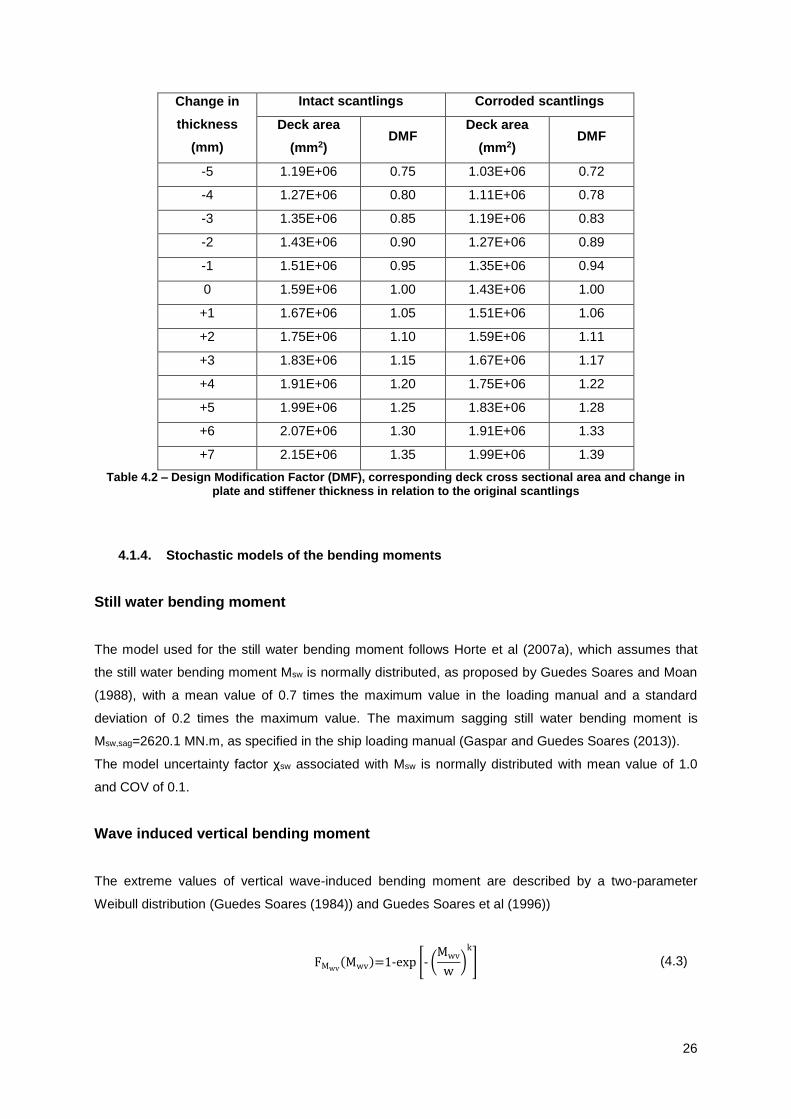
26
Change in
thickness
(mm)
Intact scantlings Corroded scantlings
Deck area
(mm2) DMF
Deck area
(mm2) DMF
-5 1.19E+06 0.75 1.03E+06 0.72
-4 1.27E+06 0.80 1.11E+06 0.78
-3 1.35E+06 0.85 1.19E+06 0.83
-2 1.43E+06 0.90 1.27E+06 0.89
-1 1.51E+06 0.95 1.35E+06 0.94
0 1.59E+06 1.00 1.43E+06 1.00
+1 1.67E+06 1.05 1.51E+06 1.06
+2 1.75E+06 1.10 1.59E+06 1.11
+3 1.83E+06 1.15 1.67E+06 1.17
+4 1.91E+06 1.20 1.75E+06 1.22
+5 1.99E+06 1.25 1.83E+06 1.28
+6 2.07E+06 1.30 1.91E+06 1.33
+7 2.15E+06 1.35 1.99E+06 1.39
Table 4.2 – Design Modification Factor (DMF), corresponding deck cross sectional area and change in plate and stiffener thickness in relation to the original scantlings
4.1.4. Stochastic models of the bending moments
Still water bending moment
The model used for the still water bending moment follows Horte et al (2007a), which assumes that
the still water bending moment Msw is normally distributed, as proposed by Guedes Soares and Moan
(1988), with a mean value of 0.7 times the maximum value in the loading manual and a standard
deviation of 0.2 times the maximum value. The maximum sagging still water bending moment is
Msw,sag=2620.1 MN.m, as specified in the ship loading manual (Gaspar and Guedes Soares (2013)).
The model uncertainty factor χsw associated with Msw is normally distributed with mean value of 1.0
and COV of 0.1.
Wave induced vertical bending moment
The extreme values of vertical wave-induced bending moment are described by a two-parameter
Weibull distribution (Guedes Soares (1984)) and Guedes Soares et al (1996))
FMwv(Mwv)=1-exp [- (
Mwv
w)
k
] (4.3)

27
with the shape parameter k=1.0, which is equivalent to assuming an exponential distribution of Mwv
(Guedes Soares and Moan (1991), Wirsching et al (1997) and Huang and Moan (2008)). The scale
parameter is determined to satisfy P[Mwv>Mwv,max]=10-8, i.e. the probability of the occurrence of
bending moments greater than the maximum vertical wave-induced moment is 10-8 (a generic small
value). The scale parameter w is given by:
w=-Mwv,max
ln10-8 (4.4)
The maximum vertical wave-induced bending moment was obtained, using the formula presented in
the IACS CSR for double hull tankers (IACS (2010)), as follows:
Mwv,max=-fprob0.11fwv-vCwvL2B(Cb+0.7) [KN.m] (4.5)
with:
fprob = 1.0
fwv-v = 1.0
Cwv=10.75- (300-L
100)
32⁄
(4.6)
The distribution for annual extreme values of vertical wave induced bending moments is then defined
as a Gumbel model, with the parameters defined from the initial Weibull distribution:
FMwve(Mwve)=exp [-exp (-
Mwve-λ
θ)] (4.7)
With Mwve a random variable that represents annual extreme values of the vertical wave-induced
bending moment. The parameters of the Gumbel distribution were defined as Guedes Soares (1984):
λ=w(ln nc)1 k⁄ (4.8)
θ=w
k(ln nc)
(1-k)k
⁄ (4.9)
where nc is the mean number of wave load cycles expected over the reference time period (Tr), for a
given operational profile of the ship and mean wave period (Tw) representative of the sea state
considered. An estimate for nc can be given by 0.35Tr/Tw.
The model uncertainty factors χwv associated with the wave-induced bending moment and χnl which
accounts for the nonlinear effects were defined as a normally distributed with mean value 1.0 and a
COV of 0.1 (Horte et al (2007a)).

28
In the present analysis the reference time considered was Tr=1.0 year and the mean wave period
Tw=8.0 s. The period of operation of the ship in fully loaded condition was 0.35Tr.
Parameter Value Units
k 1.0 -
w 339.84 MN.m
Mwv,max 6260.05 MN.m
Tr 1.0 year
Tw 8.0 s
nc 1.38e6 -
λ 4804.42 MN.m
θ 339.84 MN.m
Table 4.3 – Parameters of the stochastic model of the wave induced bending moment
Combination of still water and wave induced bending moments
The combination between the two bending moments of the hull girder is done by linear superposition.
Following the Turkstra load combination rule (Turkstra (1970)), two load combinations could be
considered:
a) An annual extreme value of the wave induced moment together with a random value of the
still water moment
b) An annual extreme of the still water moment together with an extreme value of the wave
moment during one voyage.
For the present analysis, taking into account the magnitude, the variability and the duration of the
voyage, the combination (a) was found to be governing for the probability of failure (Horte et al
(2007a)).
Variable Distribution Mean value
[MN.m]
Standard deviation
[MN.m] COV
Msw Normal 1834.1 524.0 0.29
Mwv Gumbel 5000.6 435.9 0.09
Table 4.4 – Probabilistic distributions of the still water and wave induced bending moments

29
4.2. Ultimate strength assessment
4.2.1. PCA code
In the present work the ultimate bending capacity of the cross section, Mu, was obtained using the
IACS’ progressive collapse analysis (PCA), described in 4.1.1 (IACS (2010)).
The PCA code developed by Gaspar and Guedes Soares (2013) is used. The analysis’ input involves
three files for each calculation of Mu:
o PROGRESSIVE_COLLAPSE_INPUT_DATA: this file includes information on the number of
stiffener and hard corner elements, type of curvature condition (sagging or hogging) and
other data related to the iteration process;
o STIFFENER_ELEMENTS_DATA: coordinates and thicknesses of stiffener elements and
respective material properties ;
o HARD_CORNER_ELEMENTS_DATA: coordinates and thicknesses of hard corner elements
and respective material properties.
The reliability assessment was performed considering the material properties and the thicknesses of
the midship cross section as deterministic values, considering the respective mean values presented
in Table 4.5.
Following the conclusions of Guedes Soares (1988), the material properties to be considered in the
PCA are the yield stress and the Young modulus. The uncertainties in the structural dimensions were
modelled by normal distributions with mean value equal to the design value and coefficient of variation
(COV) equal to 0.05.
The uncertainty in the yield stress is represented by a lognormal distribution and the characteristic
yield stress is defined as the 5th percentile of its distribution (Horte et al (2007a)).
Based on the studies on the uncertainty of the hull girder bending capacity performed in Harada and
Shigemi (2007), the Young modulus was assumed to be a deterministic value.
Variable Description Unit Design
value
Mean
value
Standard
deviation COV
Probability
distribution
t Plate thickness mm td td 0.05 td 0.05 Normal
tw Stiffener web tickness mm twd twd 0.05 twd 0.05 Normal
tf Stiffener flange
thickness mm tfd tfd 0.05 tfd 0.05 Normal
σyd (NS) Yield stress for normal
strength steel N/mm2 235 269 21.52 0.08 Lognormal
σyd (HS) Yield stress for high
strength steel N/mm2 315 348 20.88 0.06 Lognormal
E Young modulus N/mm2 206000 206000 - - Deterministic
Table 4.5 – Stochastic models of the material properties and thicknesses of the midship cross section

30
4.2.2. Effect of the design modification factor on the ultimate strength capacity
The results of the PCA Code are presented graphically in Figure 4.2 and Figure 4.3, where each curve
represents the resisting bending moment Mv, in sagging condition, of the midship cross section when
the hull girder is subjected to a curvature Kv. The ultimate bending capacity Mu is, by definition, the
maximum of the curve Mv vs. Kv.
In Figure 4.4 the ultimate bending capacity is given as a function of the DMF, for the cases of gross
and net original scantlings.
Figure 4.2 – Resisting moment as a function of the imposed curvature to the hull girder, considering intact scantlings and different DMF
Figure 4.3 – Resisting moment as a function of the imposed curvature to the hull girder, considering intact scantlings and different DMF
0.00E+00
5.00E+09
1.00E+10
1.50E+10
2.00E+10
2.50E+10
0.00E+00 5.00E-05 1.00E-04 1.50E-04 2.00E-04 2.50E-04 3.00E-04 3.50E-04 4.00E-04
Mv
[N.m
]
Kv [m^-1]
Intact scantlings-5mm
-4mm
-3mm
-2mm
-1mm
originalscantlings+1mm
+2mm
+3mm
+4mm
+5mm
+6mm
+7mm
0.00E+00
5.00E+09
1.00E+10
1.50E+10
2.00E+10
2.50E+10
0.00E+00 5.00E-05 1.00E-04 1.50E-04 2.00E-04 2.50E-04 3.00E-04 3.50E-04 4.00E-04
Mv
[N.m
]
Kv [m^-1]
Corroded scantlings-5mm
-4mm
-3mm
-2mm
-1mm
originalscantlings+1mm
+2mm
+3mm
+4mm
+5mm
+6mm
+7mm

31
Figure 4.4 – Ultimate bending moment as a function of the DMF for intact and corroded scantlings
4.2.3. Reliability of the hull girder
With the limit state function and stochastic models of the variables defined, the probability of failure
can now be calculated. For this task the COMREL software was used, which uses FORM for the
calculation of the reliability of the ship structure.
The COMREL software requires as input the definition of the limit state function describing the
reliability problem – g(X) – and the definition of the probabilistic models of the variables present in the
state function – Msw, Mwv, χu, χsw, χwv and χnl.
The first step of FORM consists in transformation of the basic random variables. The COMREL
software uses the Rosenblatt transformation, proposed by Hohenbichler and Rackwitz (1981). The
Rosenblatt transformation is given by:
u1=ϕ-1(F1(x1))
u2=ϕ-1(F2(x2|x1))
…
u2n=ϕ-1(Fn(xn|x1,x2,…,xn-1))
(4.1)
where Fn(xn|x1,x2,…,xn-1) is the conditional distribution function of the variable Xi.
The output of the calculations are presented in Figure 4.5 and Figure 4.6, where the reliability index
(β) and the probability of failure (Pf) are given as function of DMF, respectively.
For the calculation of β and Pf for different scantlings of the midship cross section, the only value
altered in the input was the value of the ultimate bending moment (Mu). The ultimate bending moment
0.0000E+00
5.0000E+09
1.0000E+10
1.5000E+10
2.0000E+10
2.5000E+10
0.70 0.80 0.90 1.00 1.10 1.20 1.30 1.40
Mu
[N
.m]
DMF
intact scantlings
corroded scantlings

32
is considered as deterministic and, for a specific DMF, has a corresponding Mu value, obtained with
the PCA Code (Figure 4.4).
Intact scantlings Corroded scantlings
DMF β Pf DMF β Pf
0.75 3.42 3.05E-04 0.72 2.41 7.89E-03
0.80 3.73 9.29E-05 0.78 2.77 2.73E-03
0.85 4.01 2.92E-05 0.83 3.12 8.79E-04
0.90 4.28 9.25E-06 0.89 3.44 2.86E-04
0.95 4.53 2.92E-06 0.94 3.73 9.53E-05
1.00 4.76 9.30E-07 1.00 4.01 2.96E-05
1.05 4.99 2.99E-07 1.06 4.28 9.23E-06
1.10 5.20 9.81E-08 1.11 4.53 2.90E-06
1.15 5.40 3.26E-08 1.17 4.77 9.24E-07
1.20 5.59 1.11E-08 1.22 4.99 2.99E-07
1.25 5.76 4.20E-09 1.28 5.19 1.01E-07
1.30 5.91 1.65E-09 1.33 5.37 3.78E-08
1.35 6.06 6.71E-10 1.39 5.54 1.45E-08
Table 4.6 – Probability of failure and reliability index as a function of the DMF
Figure 4.5 – Reliability index as a function of the DMF, for intact and corroded scantlings
2
2.5
3
3.5
4
4.5
5
5.5
6
6.5
0.70 0.90 1.10 1.30 1.50
β
DMF
Intact
Corroded

33
Figure 4.6 – Probability of failure as a function of the DMF, for intact and corroded scantlings
From the analysis of the results (Table 4.6) it can be noted a clear increase in the reliability of the ship
with the increase of the DMF, and consequently the lower the probability of failure. This was expected
since the higher the DMF the thicker the deck plates, i.e. the larger the deck area resisting the forces
imposed on the hull girder.
0.00E+00
1.00E-03
2.00E-03
3.00E-03
4.00E-03
5.00E-03
6.00E-03
7.00E-03
8.00E-03
9.00E-03
0.70 0.90 1.10 1.30 1.50
Pf
DMF
Intact
Corroded

34
5. Cost benefit analysis
5.1. Objectives
The ship’s optimal safety level was assessed by performing a cost benefit analysis (CBA). The
objective is to establish an optimum safety level for the Suezmax tanker ship, considering as a risk
control option (RCO) the change in deck scantlings.
The total expected cost is the sum of two distinct costs, one the cost associated with the structural
failure of the ship and the second the cost of implementing a RCO. The first term involves costs
associated with property damage, environmental pollution and loss of human life, while the second
term involves the costs related to the construction of the deck structure, where the amount of work is
connected with the amount of steel of the structure.
The methodology to obtain the optimum safety level, i.e. the optimum reliability index, followed project
SAFEDOR’s cost effectiveness analysis of oil tankers (Horte et al (2007b)).
The cost model used in the CBA is described in detail in the next sections of the report.
5.2. Cost model
The cost benefit analysis of the modification of the ship’s deck structure is given by:
Ctβt=CT f
βt +Cmeβt (5.1)
where Ctβt is the total expected cost, CT f
βt is the total cost associated with the structural failure of the
ship and Cmeβt is the cost of implementing the structural safety measure.
Each of the costs are related to a given target reliability index βt, as this influences both the cost of
failure and the cost of the RCO to achieve the safety level βt.
5.2.1. Target reliability index
To start it was defined a range of target reliability indexes, i.e. values of the reliability index (β t) at year
25 of operation of the ship, considered, for the purposes of this analysis, as the last year of the ship’s
operational life. The target values were set between 1.5 and 5, with 0.5 spacing.
The corresponding annual probability of failure (Pf) is given by:
Pf=ϕ(-βt) (5.2)
where ϕ represents the standard normal probability distribution.

35
From the results of the structural reliability analysis, the ration between the annual probabilities of
failure, associated with Net and Gross scantlings, for the original scantlings of the ship’s deck, is:
rPf=
Pfnet
Pfgross
=31.86 (5.3)
This value was used to obtain the annual probability of failure at year 0 of the ship’s operation, based
on the target reliability index, as follows:
Pfgross=rPf
∙Pfnet (5.4)
The annual probability of failure for each year of operation of the ship (t), between 1 and 25, is given
by:
Pfi=ϕ (-βgross+
(ti-1)(βgross-βnet)
24) ,i∈[1,25] (5.5)
5.2.2. Implied cost of averting a fatality
The costs related to the loss of human life, in this case loss of life of the crew members, were
accounted for using the implied cost of averting a fatality (ICAF).
Instead of using the value of 3 million US$ as proposed by Skjong et al (2005), the value of ICAF used
in the risk model was obtained from the average of OCDE countries during a period of 16 years
starting from 1995 (OCDE (2014)). This represents an update of the value reported in Skjong et al
(2005), given that the amount of information gathered was sufficient to obtain an estimation of the
ICAF value, by considering the statistics in OCDE countries for the life expectancy at birth (e) and the
gross domestic product (GDP) per capita (g) from 1995 to 2011.
ICAF=7∙ge
4 (5.6)

36
Year Life expectancy at birth (e)
[years]
GDP per capita (g)
[US$]
ICAF
[106 US$]
1995 75.73 20337.05 2.74
1996 76.13 20701.48 2.80
1997 76.41 19724.75 2.68
1998 76.61 19798.54 2.69
1999 76.80 20353.20 2.77
2000 77.13 19756.06 2.70
2001 77.44 19514.97 2.68
2002 77.64 21108.14 2.90
2003 77.78 25274.99 3.48
2004 78.27 28953.40 4.02
2005 78.47 31031.00 4.31
2006 78.84 33046.59 4.61
2007 78.98 37893.57 5.29
2008 79.28 40456.22 5.67
2009 79.55 35914.74 5.05
2010 79.77 37341.10 5.22
2011 80.04 40984.68 5.76
Average ICAF between 1995-2011 in OCDE countries 3.85
Table 5.1 – Life expectancy at birth, GDP per capita and ICAF for OCDE countries from 1995 to 2011
5.2.3. Cost of averting a ton of oil spilt
In the present analysis it is considered a value of CATS of 60 000 US$. A FSA study on crude oil
tankers that used this criterion of 60 000 US$ per ton was conducted by project SAFEDOR and
submitted to IMO by Denmark (IMO (2008)).
The criterion used in the current work is representative of a spill of a generic oil product in a generic
geographical area.
5.2.4. Cost of implementing a safety measure
In the present analysis, the cost of implementing a safety measure only accounts for the modification
of the deck structure, more specifically the cost of steelwork. Depending on the DMF the value of 𝐶𝑚𝑒𝛽𝑡
is positive or negative if DMF is larger or smaller than 1, respectively.
Cmeβt =(DMFβt-1)∙Wsteel∙Csteelwork/ton (5.7)

37
where:
Wsteel is the weight of the cylindrical body of the ship, assumed as 40% of Lpp
Csteelwork/ton is the cost of steelwork per ton of steel
DMFβt is the design modification factor associated with βt
Variables / parameters Value Unit
Wsteel 1418.69 ton
Csteelwork/ton 2500 US$
Table 5.2 – Variables and parameters associated with the cost of implementing a RCO
5.2.5. Cost associated with the structural failure of the ship
The cost associated with the structural failure of the ship includes the property costs, i.e. loss of the
ship and loss of cargo, the environmental pollution costs, i.e. the clean-up costs associated with the
spillage of oil, and costs associated with the loss of human life, i.e. the loss of life of crew members.
The cost of structural failure of the ship is related to the reliability of the ship structure, as each
reliability index corresponds to a probability of failure, affecting the costs associated with the different
types of risk.
The cost associated with the structural failure of the ship is calculated considering the operational life
of the ship T, assumed to be 25 years for the present work; and a discount rate γ of 5%.
CT fβt = ∑ Pf(βt)[Cn(t)+(Cc+Cd+Cv)]e-γt
T
t=1
(5.8)
where:
Pf is the annual probability of failure
Cn(t) is the cost of the ship in the year t
Cc is the cost associated with the loss of cargo
Cd is the cost of accidental spill
Cv is the cost associated with loss of human life
Ship cost
The cost of the ship is a function of the ship’s age, as such the cost of the ship at year 0 is the initial
cost of the ship and at year 25 is the scrapping value.
Cn(t)=Cn0-(Cn0
-Cscrap)∙ (t
25) (5.9)
where:
Cn0is the initial cost of the ship
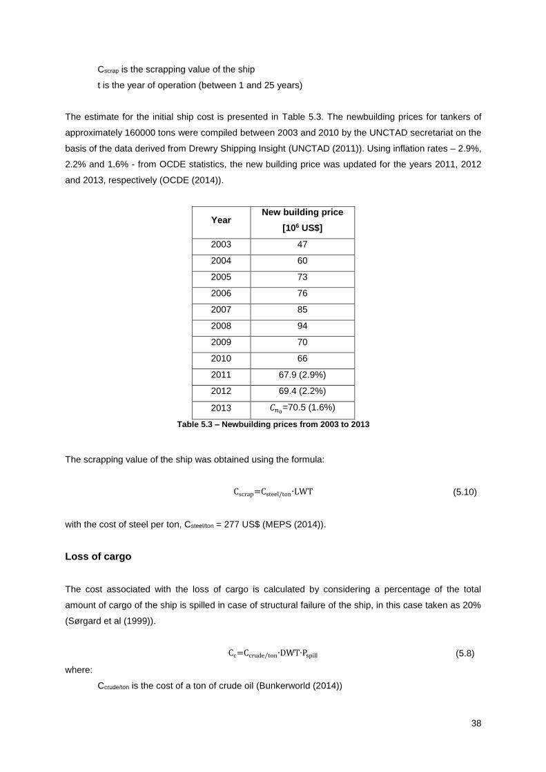
38
Cscrap is the scrapping value of the ship
t is the year of operation (between 1 and 25 years)
The estimate for the initial ship cost is presented in Table 5.3. The newbuilding prices for tankers of
approximately 160000 tons were compiled between 2003 and 2010 by the UNCTAD secretariat on the
basis of the data derived from Drewry Shipping Insight (UNCTAD (2011)). Using inflation rates – 2.9%,
2.2% and 1.6% - from OCDE statistics, the new building price was updated for the years 2011, 2012
and 2013, respectively (OCDE (2014)).
Year New building price
[106 US$]
2003 47
2004 60
2005 73
2006 76
2007 85
2008 94
2009 70
2010 66
2011 67.9 (2.9%)
2012 69.4 (2.2%)
2013 𝐶𝑛0=70.5 (1.6%)
Table 5.3 – Newbuilding prices from 2003 to 2013
The scrapping value of the ship was obtained using the formula:
Cscrap=Csteel/ton∙LWT (5.10)
with the cost of steel per ton, Csteel/ton = 277 US$ (MEPS (2014)).
Loss of cargo
The cost associated with the loss of cargo is calculated by considering a percentage of the total
amount of cargo of the ship is spilled in case of structural failure of the ship, in this case taken as 20%
(Sørgard et al (1999)).
Cc=Ccrude ton⁄ ∙DWT∙Pspill (5.8)
where:
Ccrude/ton is the cost of a ton of crude oil (Bunkerworld (2014))

39
Pspill is the percentage of cargo spilled in case of structural failure of the ship
Parameters/Variables Value Unit
Ccrude/ton 108 US$
Pspill 1/5 -
Table 5.4 – Parameters and variables associated with the cost of loss of cargo
Accidental oil spill
In case of structural failure of the ship structure there is a 20% chance of oil being spilt, of that amount
it is considered a 10% chance of the oil reaching the shoreline (Sørgard et al (1999)). This means that
in case of an accidental oil spill, 10% of the spill will need to be “dealt with”, meaning it will need to be
cleaned up, which will involve costs; costs that are here taken into account by considering the CATS
criterion.
Cd=Pspill∙Psl∙CATS∙DWT (5.9)
where:
CATS is the Cost of Averting a Ton of oil Spilt
Psl is the probability of the oil spilt reaching the shoreline
Variables Value Units
CATS 60000 US$
Psl 10 %
Table 5.5 – Variables associated with the cost of an accidental oil spill
Loss of human life
In a cost benefit analysis the loss of human life is accounted for by including a CAF index, in this case
the ICAF, in the objective function.
Teixeira (2007) compiled data from the U.S. Department of Transportation from 2003, where the
average number of crew members of an oil tanker of 110 to 175 DWT is 25 members.
The probability of loss of crew was assumed to be 25%, as used in a study of a Suezmax tanker
performed by SAFEDOR (Horte et al (2007b)).
Cv=ncrew∙Pcrew∙ICAF (5.10)
where:
ncrew is the number of crew members
Pcrew is the probability of loss of life of a crew member in case of an accident
ICAF is the Implied Cost of Averting a Fatality

40
Variables Value Units
ncrew 25 -
Pcrew 25 %
ICAF 3.85 106 US$
Table 5.6 – Variables associated with the cost related to the loss of human life
5.3. Optimal reliability index
The objective of the cost benefit analysis is to obtain the optimal safety level of the ship’s structure.
Now that the cost model and all the variables and parameters have been defined, the optimum
reliability index is obtained by minimizing the objective function (equation (5.1)).
The initial analysis was performed for target reliability indexes between 1.5 and 5, with an interval of
0.5, however, given the result of the analysis and with the intent of increasing the precision of the
value of βopt, within the previously described range of values for βtarget, the values between 3 and 4.5
were taken in intervals of 0.02.
The optimum reliability index, using the new intervals, is shown in Figure 5.1, where βopt is 3.52,
corresponding to the minimum of the curve of total expected cost (Ct).
Figure 5.1 – Total expected cost as a function of the reliability index
-1.00E+00
-8.00E-01
-6.00E-01
-4.00E-01
-2.00E-01
0.00E+00
2.00E-01
4.00E-01
6.00E-01
8.00E-01
1.00E+00
3.00 3.50 4.00 4.50
10^
6 U
S$]
β opt
Ctf
Cme
Ct

41
5.4. Parametric studies
In the cost analysis performed previously, the input variables have a fixed value, meaning that the
optimum reliability index obtain is only representative of that specific set of conditions, including costs,
probabilities and other assumptions.
The objective of the present section is to carry out a parametric analysis of the input variables of the
cost model, in order to ascertain the influence of these variables in the outcome of the cost analysis.
The procedure consists of varying the value of one of the input variables, while keeping the others with
their initial values, and obtaining the optimum reliability index for each variation. This process is
repeated for each input variable (Table 5.7) and a relation is obtained between the variation of the
initial value of the variable and the optimum safety level.
Designation Input variable Initial value Units
Cost of steelwork per ton C_steelwork/ton 0.0025 [106 US$]
Cost of cargo (crude oil) per ton C_crude/ton 108 [US$]
Cost of steel per ton C_steel/ton 277 [US$]
Initial cost of the ship C_n0 70.5 [106 US$]
Implied cost of averting a fatality ICAF 3.85 [106 US$]
Probability of loss of crew P_crew 0.25 [-]
Number of crew members n_crew 25 [-]
Cost of averting a ton of oil spilt CATS 0.06 [106 US$]
Probability of spill reaching the shoreline P_sl 0.1 [-]
Probability of oil spill P_spill 0.2 [-]
Table 5.7 – Input variables of the cost model
5.4.1. CATS
The input variable CATS was set from 40000 to 100000 US$, in intervals of 5000 US$, and the
resulting optimum reliability index was taken from the model. Figure 5.2 shows the mentioned points
and the linear regression using these points.
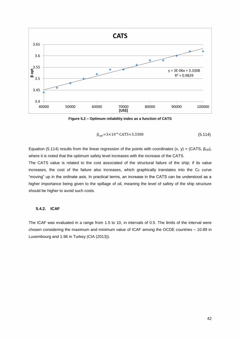
42
Figure 5.2 – Optimum reliability index as a function of CATS
βopt=3×10⁻⁶∙CATS+3.3308 (5.114)
Equation (5.114) results from the linear regression of the points with coordinates (x, y) = (CATS, βopt),
where it is noted that the optimum safety level increases with the increase of the CATS.
The CATS value is related to the cost associated of the structural failure of the ship; if its value
increases, the cost of the failure also increases, which graphically translates into the Ctf curve
“moving” up in the ordinate axis. In practical terms, an increase in the CATS can be understood as a
higher importance being given to the spillage of oil, meaning the level of safety of the ship structure
should be higher to avoid such costs.
5.4.2. ICAF
The ICAF was evaluated in a range from 1.5 to 10, in intervals of 0.5. The limits of the interval were
chosen considering the maximum and minimum value of ICAF among the OCDE countries – 10.89 in
Luxembourg and 1.96 in Turkey (CIA (2013)).
y = 3E-06x + 3.3308R² = 0.9829
3.4
3.45
3.5
3.55
3.6
3.65
40000 50000 60000 70000 80000 90000 100000
β o
pt
[US$]
CATS

43
Figure 5.3 – Optimum reliability index as a function of ICAF
βopt=0.0065∙ICAF+3.4879 (5.15)
The increase in ICAF results in an increase of the optimum reliability index. Although not in the same
measure, the effect of the ICAF is comparable to that of the CATS, but in this case the focus is on the
avoidance of human casualties.
5.4.3. Cost of steelwork per ton
The range of values for cost of steelwork per ton was from 1000 to 4000 US$.
Figure 5.4 – Optimum reliability index as a function of the cost of steelwork per ton
βopt=-10-4∙Csteelwork/ton+3.8164 (5.16)
y = 0.0065x + 3.4879R² = 0.8997
3.49
3.5
3.51
3.52
3.53
3.54
3.55
3.56
3.57
1.5 2.5 3.5 4.5 5.5 6.5 7.5 8.5 9.5
β o
pt
[10^6 US$]
ICAF
y = -0.0001x + 3.8164R² = 0.9679
3.30
3.35
3.40
3.45
3.50
3.55
3.60
3.65
3.70
3.75
3.80
1000 1500 2000 2500 3000 3500 4000
βo
pt
[US$]
C_steelwork/ton

44
The linear regression of the points with coordinates (x, y) = (Csteelwork/ton, βopt) indicates the decrease of
the reliability index with the increase of the cost of steelwork.
The cost of steelwork per ton influences the cost associated with the safety measure, meaning the
higher the cost of the steelwork the higher the cost of the safety measure, which graphically means
the Cme curve “moves” upward.
From a practical stand point, an increase in the cost of steelwork would cause, considering that all
other aspects of the cost model are kept constant, the thickness of the deck to be lower and therefore
the safety level would be also lower.
5.4.4. Initial ship cost
The initial cost of the ship was changed from 10 to 250 million US$.
Figure 5.5 – Optimum reliability index as a function of the initial ship cost
βopt=3×10⁻⁴∙Cn0+3.4952 (5.17)
Looking at Figure 5.5, the linear regression of the points with coordinates (x, y) = (Cn0, βopt) resulted in
a straight line with positive slope, i.e. the reliability index increases with the increase in initial ship cost.
The initial ship cost influences the cost of loss of the ship, which in turn influences the total structural
failure cost. Since the cost associated with a safety measure is constant, the total expected cost varies
only due to the cost of failure.
Graphically, an increase/decrease in initial ship cost results in an upward/downward “shift” of the total
failure cost, and consequently minimum of the total expected cost curve “moves” right/left.
In practice, if the initial cost of the ship is higher, then the cost of loss of ship is also higher, and in
order to avoid incurring in a loss of higher value the safety level will also be set higher.
y = 0.0003x + 3.4952R² = 0.9222
3.49
3.5
3.51
3.52
3.53
3.54
3.55
3.56
3.57
3.58
10 60 110 160 210
βo
pt
[10^6 US$]
C_n0
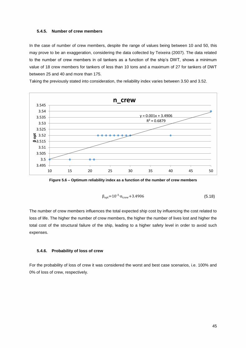
45
5.4.5. Number of crew members
In the case of number of crew members, despite the range of values being between 10 and 50, this
may prove to be an exaggeration, considering the data collected by Teixeira (2007). The data related
to the number of crew members in oil tankers as a function of the ship’s DWT, shows a minimum
value of 18 crew members for tankers of less than 10 tons and a maximum of 27 for tankers of DWT
between 25 and 40 and more than 175.
Taking the previously stated into consideration, the reliability index varies between 3.50 and 3.52.
Figure 5.6 – Optimum reliability index as a function of the number of crew members
βopt=10-3∙ncrew+3.4906 (5.18)
The number of crew members influences the total expected ship cost by influencing the cost related to
loss of life. The higher the number of crew members, the higher the number of lives lost and higher the
total cost of the structural failure of the ship, leading to a higher safety level in order to avoid such
expenses.
5.4.6. Probability of loss of crew
For the probability of loss of crew it was considered the worst and best case scenarios, i.e. 100% and
0% of loss of crew, respectively.
y = 0.001x + 3.4906R² = 0.6879
3.495
3.5
3.505
3.51
3.515
3.52
3.525
3.53
3.535
3.54
3.545
10 15 20 25 30 35 40 45 50
β o
pt
n_crew

46
Figure 5.7 – Optimum reliability index as a function of the probability of loss of crew
βopt=10-3∙Pcrew+3.4864 (5.19)
The logic for analysing the influence of the probability of loss of crew in the variation of the reliability
index is the same as for the number of crew members. The higher the probability of loss of life, higher
the costs in case of structural failure related to the loss of human life, and, as such, the higher the
safety level in order to avoid it.
5.4.7. Cost of steel per ton
The range of values for the cost of steel per ton was set between 10% and 500% of the initial value,
just as a reference for considering a very small value and a much higher one.
Figure 5.8 – Optimum reliability index as a function of the cost of steel per ton
y = 0.001x + 3.4864R² = 0.9679
3.46
3.48
3.5
3.52
3.54
3.56
3.58
3.6
0 10 20 30 40 50 60 70 80 90 100
β o
pt
[%]
P_crew
y = 2E-05x + 3.511R² = 0.6598
3.495
3.5
3.505
3.51
3.515
3.52
3.525
3.53
3.535
3.54
3.545
25 225 425 625 825 1025 1225
β o
pt
[US$]
C_steel/ton

47
βopt=2×10⁻⁵∙Csteel/ton+3.511 (5.20)
The cost of steel per ton affects the scrapping value of the ship, which affects the cost of loss of ship,
which affects the total cost of structural failure, in the sense that if the first increases the last
increases.
In practical terms, if the cost of steel is higher, which means the cost of loss of ship is higher, then the
safety level will also be higher to prevent incurring in higher monetary losses.
5.4.8. Probability of cargo spilt in case of accident
In case of structural failure of the ship structure, the probability of cargo being spilt, will dictate the
costs of loss of cargo and to some extent the costs of clean up. For the range of values it was
considered the two extreme situations that may occur, the worst, where there is complete loss of
cargo (Pspill=100%), and the best, where no cargo is spilt (Pspill=0%).
Figure 5.9 – Optimum reliability index as a function of the probability of spilling oil in case of structural failure
βopt=2×10⁻⁶∙Pspill3-0.0004∙𝑃𝑠𝑝𝑖𝑙𝑙
2+0.0264𝑃𝑠𝑝𝑖𝑙𝑙+3.0978 (5.21)
A different approach was taken when analysing the results from this study, instead of a linear
regression, the points were approximated by a third order polynomial function.
The greater the spillage of oil, the higher the cost of loss of cargo and the costs related to clean up of
the spill, consequently the tendency will be for the safety level to be higher to avoid these expenses.
y = 2E-06x3 - 0.0004x2 + 0.0264x + 3.0978R² = 0.988
3
3.2
3.4
3.6
3.8
4
0 10 20 30 40 50 60 70 80 90 100
β o
pt
[%]
P_spill

48
5.4.9. Probability of cargo spilt reaching the shoreline
The rationale behind the choice of range of values for the probability of cargo spilt reaching the
shoreline mimics the one for the probability of cargo spilt. The values were set between 0 and 100%.
Figure 5.10 – Optimum reliability index as a function of the probability of the spilt oil reaching the shoreline
βopt=2×10⁻⁶∙𝑃𝑠𝑙3-0.0005∙𝑃𝑠𝑙
2+0.0339∙Psl+3.1387 (5.22)
As in the previous study of the probability of cargo spilt, the data from the current parametric analysis
was approximated by a third order polynomial function.
The probability of cargo reaching the shoreline affects the cost related to the clean up of the spill,
when the former is higher the latter is also higher. The reliability index is higher when the probability of
cargo reaching the shoreline is higher, as it is economically (and in practical terms, environmentally)
appealing to avoid higher costs.
5.5. Sensitivity analysis
In the present chapter a sensitivity analysis was carried out by increasing the value of each one of the
input variables by 10%, while keeping the others constant, and obtaining the variation, in terms of
percentage, of the reliability index.
Following this approach, the Figure 5.11 was obtained. From this bar chart, the input variables of
higher influence on the reliability index are, in descending order, the cost of steelwork per ton
(Csteelwork/ton); the CATS, the probability of cargo spill (Pspill) and the probability of cargo reaching the
shoreline (Psl) with equal effect; and the cost of cargo per ton (Ccrude/ton), the cost of steel per ton
(Csteel/ton), the initial cost of the ship (Cn0), the ICAF, the probability of loss of crew (Pcrew) and the
number of crew members (ncrew) with no effect on the optimum reliability index.
y = 2E-06x3 - 0.0005x2 + 0.0339x + 3.1387R² = 0.9784
3
3.2
3.4
3.6
3.8
4
0 10 20 30 40 50 60 70 80 90 100
β o
pt
[%]
P_sl

49
These results can be explained by the fact that the target reliability index is calculated in intervals of
0.02, meaning that there would have to be at least 0.57% variation to change the value of the reliability
index, considering that the initial optimum reliability index is 3.52.
Designation Units Initial value 10% increase
C_steelwork/ton [10^6 US$] 0.0025 0.00275
C_crude/ton [US$] 108 118.8
C_steel/ton [US$] 277 304.7
C_n0 [10^6 US$] 70.5 77.55
ICAF [10^6 US$] 3.85 4.235
P_crew [-] 0.25 0.275
n_crew [-] 25 27.5
CATS [10^6 US$] 0.06 0.066
P_sl [-] 0.1 0.11
P_spill [-] 0.2 0.22
Table 5.8 – Input variables: initial values and 10% increase
Figure 5.11 – Percentage change of optimum reliability index when increasing the initial value of the input variable by 10%
In order to better understand the influence of each input variable model equations obtained from a
linear or cubic regressions applied to data generated from the parametric studies were developed.
Using this approach, the methodology is the same: increasing the initial value of the input variables by
10% and evaluating the change in the optimum safety level.
The results of the sensitivity analysis are presented in Figure 5.12. This approach allowed for the
differentiation between the effects of each input variable in the optimization of the objective function,
-1.1364
0.0000 0.0000 0.0000 0.0000 0.0000 0.0000
0.5682 0.5682 0.5682
-1.40
-1.20
-1.00
-0.80
-0.60
-0.40
-0.20
0.00
0.20
0.40
0.60
0.80
%
β optimum vs. Input variable

50
according to which the variables that cause the greater variation in the optimum reliability index are, in
descending order: Pspill, Csteelwork/ton, Psl, CATS, ICAF, ncrew, Cn0, Csteel/ton, Pcrew and Ccrude/ton.
The cost of cargo per ton (or crude oil per ton) yielded in both sensitivity analysis a 0% variation of the
reliability index. This input variable was also analysed in the parametric studies, but the results were
not presented, since, within a wide range of cost values, the value of the optimum reliability index was
constant.
Figure 5.12 – Percentage change of optimum reliability index when increasing the initial value of the input variable by 10% based on the equations obtained from the parametric studies
0.7020
0.5182 0.5127
0.0712 0.0711 0.06010.0158 0.0007
-0.7010-0.8000
-0.7000
-0.6000
-0.5000
-0.4000
-0.3000
-0.2000
-0.1000
0.0000
0.1000
0.2000
0.3000
0.4000
0.5000
0.6000
0.7000
0.8000
β optimum vs. Input variable

51
6. Uncertainty analysis
6.1. Monte Carlo simulation
In chapter 5 all input variables were assumed as deterministic values, i.e. the initial values assigned to
each one were constant, and the optimum reliability index was also unique and representative of that
specific cost model.
In the present chapter the objective is to obtain the optimum reliability index considering the
uncertainties in the input variables, meaning that rather than assuming a fixed value for a variable,
each variable will be represented by a probabilistic model and the result of the optimum safety level
will also be described by a probabilistic model reflecting the aspect of the uncertainties in the input
variables.
For this task the @Risk tool from Palisade for Monte Carlo simulation was used, starting with the
definition of the probability distributions of the input variables and setting the optimum reliability index
as output of the cost model.
6.2. Stochastic models
The stochastic models of the input variables are presented in Table 6.1. Three of the input variables –
Csteel/ton, Ccrude/ton and Pcrew – were assumed to be deterministic, given the results of the sensitivity
analysis in chapter 5, where the variation of the reliability index is lower than 0.02%.
For the remaining variables, the stochastic models are based on triangular distributions with the most
likely value equal to the initial (fixed) value.
Input variables Distribution Minimum value Most likely value Maximum value Units
P_spill Triangular 10 20 30 [%]
C_steelwork/ton Triangular 1000 2500 4000 [US$]
P_sl Triangular 5 10 20 [%]
CATS Triangular 40000 60000 100000 [US$]
ICAF Triangular 1.96 3.85 10.89 [106 US$]
n_crew Triangular 20 25 30 [-]
C_n0 Triangular 50 70.5 100 [106 US$]
C_steel/ton deterministic 277 277 277 [US$]
P_crew deterministic 25 25 25 [%]
C_crude/ton deterministic 108 108 108 [US$]]
Table 6.1 – Stochastic models of the input variables
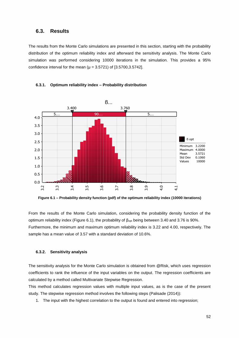
52
6.3. Results
The results from the Monte Carlo simulations are presented in this section, starting with the probability
distribution of the optimum reliability index and afterward the sensitivity analysis. The Monte Carlo
simulation was performed considering 10000 iterations in the simulation. This provides a 95%
confidence interval for the mean (μ = 3.5721) of [3.5700,3.5742].
6.3.1. Optimum reliability index – Probability distribution
Figure 6.1 – Probability density function (pdf) of the optimum reliability index (10000 iterations)
From the results of the Monte Carlo simulation, considering the probability density function of the
optimum reliability index (Figure 6.1), the probability of βopt being between 3.40 and 3.76 is 90%.
Furthermore, the minimum and maximum optimum reliability index is 3.22 and 4.00, respectively. The
sample has a mean value of 3.57 with a standard deviation of 10.6%.
6.3.2. Sensitivity analysis
The sensitivity analysis for the Monte Carlo simulation is obtained from @Risk, which uses regression
coefficients to rank the influence of the input variables on the output. The regression coefficients are
calculated by a method called Multivariate Stepwise Regression.
This method calculates regression values with multiple input values, as is the case of the present
study. The stepwise regression method involves the following steps (Palisade (2014)):
1. The input with the highest correlation to the output is found and entered into regression;

53
2. The partial correlation coefficient of every input that is not in regression with the response is
calculated, and the variable with the largest correlation value is entered into regression;
3. A regression equation is created for every input that has been entered into regression. An F-
test is used for each input variable, leading to the removal of “insignificant” variables from
regression.
4. Steps 2 and 3 are repeated until the only remaining variables have been rejected from
regression.
5. A final regression equation is calculated from the “not rejected” input variables. The
coefficients obtained from this regression are listed in the sensitivity report.
The results of the sensitivity analysis are presented in tornado graphs, where the longer the bar (larger
the coefficient), the greater the impact the input variable has on the output. A positive/negative
coefficient indicates a positive/negative impact, i.e. increasing this input will increase/decrease the
output. The coefficients listed in sensitivity report are normalized by the standard deviation of the
output and the standard deviation of that input (Palisade (2014)).
Figure 6.2 – Regression coefficients of the input variables (10000 iterations)
The sensitivity analysis (Figure 6.2) ranks the input variables from most influential to least. Noting that
the cost of steelwork has a negative impact, meaning an increase of this variable leads to a decrease
in the reliability index, whilst the other input variables have a positive impact on the output.
Despite not being directly comparable, the results from this sensitivity analysis are congruent with the
ones obtained from the previous analysis in chapter 5, as regards to the influence of the input
variables, ranking the Csteelwork/ton, Pspill, Psl and CATS as the most influential and the ICAF, Cn0 and
ncrew as the least.

54
6.4. Volume dependent CATS
The cost model developed throughout the current project was based on a constant value of CATS,
however given the importance of this variable in the outcome of the analysis, i.e. the influence of
CATS in the value of the optimum reliability level, and the recent developments on environmental
criteria at the IMO level, the present chapter will consider a volume dependent CATS.
The basis for establishing the CATS value was the regression formulae from the revised guidelines for
FSA (IMO (2013)):
TSC=67275V0.5893 for all spills (6.1)
where:
CATS(V)=TSC
V=
67275V0.5893
V (6.1)
with the spill size (V) is:
V=DWT∙Pspill∙Psl (6.2)
Figure 6.3 – Cost of Averting a Ton of oil Spilled (CATS) versus the volume of the spill for V ≥ 1 ton
The value of CATS was obtained by considering the initial values of the input variables Pspill and Psl of
20% and 10%, respectively. Resulting in a CATS of 2400 US dollars.
In the previous model, used in the Monte Carlo simulation, the CATS was modelled by a triangular
distribution with minimum, most likely and maximum value of 40000, 60000 and 100000 US dollars,
respectively; in this chapter the stochastic model for the variable CATS is a triangular distribution with
0
10000
20000
30000
40000
50000
60000
70000
80000
1 10 100 1000 10000 100000
CA
TS [
US$
/to
n]
Spill weight [Ton]
CATS vs CATS (V)
constant CATS
Volume dependent CATS

55
a most likely value equal to the initial value of 2400 US$, as previously, and the minimum and
maximum value equal to 1600 and 4000 US$, by considering the same ratio minimum/most likely and
maximum/most likely, respectively, as in chapter 5.
Input variables Distribution Minimum value Most likely value Maximum value Units
P_spill Triangular 10 20 30 [%]
C_steelwork/ton Triangular 1000 2500 4000 [US$]
P_sl Triangular 5 10 20 [%]
CATS Triangular 1600 2400 4000 [US$]
ICAF Triangular 1.96 3.85 10.89 [106 US$]
n_crew Triangular 20 25 30 [-]
C_n0 Triangular 50 70.5 100 [106 US$]
C_steel/ton deterministic 277 277 277 [US$]
P_crew deterministic 25 25 25 [%]
C_crude/ton deterministic 108 108 108 [US$]]
Table 6.2 – Stochastic models of the input variables (volume dependent CATS)
6.4.1. Uncertainty analysis considering a volume dependent CATS
The results are homologous to the obtained in chapter 5, with the probability density function of the
optimum reliability index in Figure 6.4 and the sensitivity analysis in Figure 6.5. As before, it was
considered 10000 iterations in the Monte Carlo simulation.
Figure 6.4 – Probability density function of optimum reliability index (10000 iterations) (volume dependent CATS)

56
Figure 6.5 – Regression coefficients of the input variables (10000 iterations) (volume dependent CATS)
6.4.2. Constant CATS vs volume dependent CATS
The mean of the probability density function of the optimum reliability index in the case of a volume
dependent CATS is approximately 10.6% lower than with constant CATS, noting that the minimum
and maximum values and standard deviation are also lower.
As for the sensitivity analysis, there is a clear decrease in the influence of CATS on the output.
Furthermore the ranking of the influence of the input variables changed significantly, being the
predominant variables the cost of steelwork per ton and the ICAF and the remaining variables having
similar influence on the output.
Considering the initial values of CATS – 60000 and 2400 US$ - for a spill of 3326 tons (volume
reaching the shoreline), the volume dependent CATS is 4% of the constant CATS, representing an
obvious difference in costs. For the volume dependent CATS to be equivalent to the constant CATS
the volume of the spill should be around 1.25 tons.
The formulae adopted by the IMO in step 4 of FSA (IMO (2013)) describe the CATS decreasing with
the increase of oil spill size (equation 2.12), meaning the CATS is higher for smaller spills. Considering
these formulae the constant CATS is clearly inadequate to deal with large spills, attributing a value
50% lower for a spill of 5 tons and the discrepancy increases with greater spills.

57
7. Conclusions and future work
7.1. Conclusions
The way safety is being dealt with is changing, becoming a key aspect in the ship design process with
serious economic repercussions. In the last two decades there has been an increasing tendency to
adopt a more holistic and proactive approach to safety, with the introduction and development of
Formal Safety Assessment (FSA) and Goal-based standards (GBS) at IMO.
As part of the FSA methodology, cost effectiveness analysis (CEA) and cost benefit analysis (CBA)
allow the balancing of risk and costs in the design process, where risk encompasses property
damages, environmental pollution and the loss of human life.
The objective of the current work has been to develop a risk based approach for structural design of a
double hull Suezmax tanker. The assessment of the hull girder reliability was performed using
Progressive Collapse Analysis (PCA) to obtain the ultimate strength of the hull girder and First Order
Reliability Methods (FORM) to obtain the probability of failure of the hull girder.
In the risk based approach through cost benefit analysis to obtain the optimum safety level of the ship
structure, a cost model was developed considering risk criteria, namely for human life and
environmental pollution. The environmental pollution was only considered related to oil spills, in
particular the definition of the CATS criterion.
Furthermore the analysis only considered as risk control option (RCO) the change in the scantlings of
the deck structure, more specifically the change in thickness of the deck plating and stiffeners,
represented by a Design Modification Factor (DMF).
The study of the effect of the DMF on the ultimate bending capacity of the midship cross section was
carried out in chapter 4. From the results of the PCA, the ultimate bending capacity increases linearly
with the increase of the DMF, i.e. the increase of plate and stiffener thicknesses. These results reflect
the increase of the capacity of the midship cross section to support higher bending moments if the
thickness of the plates and stiffeners is higher.
Also in chapter 4 the reliability of the hull girder was calculated and presented as a function of the
DMF. The results show increasing reliability index with the increase of the DMF. For intact scantlings
the range of values goes from a DMF of 0.75 corresponding to a reliability index (β) of 3.42 to a DMF
of 1.35 corresponding to β = 6.06; for corroded scantlings the interval of DMF values starts at 0.72
corresponding to β = 2.41 to 1.39 corresponding to β = 5.54.
In chapter 5 a cost-benefit analysis was performed leading to an optimum reliability index of 3.52. Also
a sensitivity analysis was performed for the cost-benefit model considering the input variables as
deterministic values. The results of this analysis yielded the ranking of the input variables from higher
influence on the output of the model to least influential: probability of oil spill in case of accident (Pspill),
cost of steelwork per ton (Csteelwork/ton), probability of spilled oil reaching the shoreline (Psl), Cost of
Averting a Ton of oil Spilled (CATS), Implied Cost of averting A Fatality (ICAF), number of crew

58
members (ncrew), initial ship cost (Cn0), cost of steel per ton (Csteel/ton), probability of loss of life of a crew
member (Pcrew) and cost of cargo per ton (Ccrude/ton).
In chapter 6 Monte Carlo simulation is used considering the optimum reliability index as an output
variable and uncertainty and sensitivity analyses are carried out. From the Monte Carlo simulation, the
optimum reliability index has a 90% probability of being between 3.40 and 3.76.
From the results obtained from the sensitivity analysis it becomes clear that the definition of the CATS
criterion is of great importance, given that the threshold value of CATS proposed by Skjong et al
(2005) of 60000 US$ for the implementation of RCO’s is one of the determining factors on the
structural safety level of the ship, while the volume dependent CATS criterion, being now applied in
step 4 of the FSA, is considerably lower for spills greater than 5 tons (less than 50%), and therefore
much less influential in the outcome of the model results.
7.2. Recommendations for future work
Loss of human life and, in today’s society, environmental damage are very important issues in any
commercial or industrial activity. In the shipping industry the consequences of underestimating these
risks can be catastrophic and may influence the way the ships are designed and operated.
The studies carried out in this project were limited to the case study of a Suezmax tanker and to a
specific accident scenario (hull girder failure), from which it became clear that the definition of risk
criteria is a paramount subject. Moreover this kind of analysis should not be directed only at tanker
ships, despite the obvious interest when it comes to environmental pollution, or at passenger ships,
when it relates to criteria for human life.
On the wake of the current project it is suggested further homologous studies focusing on different
ship types and in depth analysis of the effects of risk criteria on the structural safety level.
Also, more detailed probabilistic models should be developed for the main parameters of the cost-
benefit model to obtain representative optimal safety levels applicable to different ship types and other
failure scenarios.

59
References
Breinholt, C., Hensel, W., Perez de Lucas, A., Sames, P.C., Skjong, R., Strang, T. and Vassalos, D.,
(2007), Risk based ship and ship system design and their approval, Proceedings of RINA Conference
on Developments in Classification and International Regulations, London, UK
Breinholt, C., Ehrke, K.-C., Papanikolaou, A., Sames, P. C., Skjong, R., Strang, T., Vassalos, D. and
Witolla, T., (2012), SAFEDOR – the implementation of risk-based ship design and approval, Procedia
– Social and behavioural sciences, Vol. 48, pp. 753-764
Breitung, K., (1984), Asymptotic approximations for multi-normal integrals, Journal of Engineering
Mechanics Division, ASCE, No. 3, Vol. 110, pp. 357-366
Bunkerworld, (2014), http://www.bunkerworld.com/prices/
CIA, (2013), The World Factbook, https://www.cia.gov/library/publications/the-world-factbook/
Cornell, C.A., (1969), A Probability Based Structural Code, American Concrete Institute Journal,
Vol.66, pp. 974-985
Davies, O.L. and Goldsmith, P.L., (1976), Statistical Methods in Research and Production, Chapter 8
Der Kiureghian, A. and Liu, P.-L., (1986), Structural reliability under incomplete probability information,
Journal of Engineering Mechanics, Journal of Engineering Mechanics Division, ASCE, No. 1, Vol. 112,
pp. 85-104
Ditlevsen, O.D., (1973), Structural reliability and the invariance problem, Research Report No. 22,
Solid Mechanics Division, University of Waterloo
Ditlevsen, O., (1981), Principle of normal tail approximation, Journal of Engineering Mechanics,
Journal of Engineering Mechanics Division, ASCE, No. 6, Vol. 107, pp. 1191-1209
Ditlevsen, O., (2004), Life Quality Index revised, Structural Safety, Vol. 26, Issue 4, pp. 443-451
Ditlevsen, O. and Friis-Hansen, (2005), Life Quality Time Allocation Index – an equilibrium economy
consistent version of the current Life Quality Index, Structural Safety, Vol. 27, Issue 3, pp. 262-275
DMA & RDANH, (2002), Risk analysis of navigational safety in Danish waters, Maritime Autority and
Royal Danish Administration of Navigation and Hydrography, Report no. P-054380-2
DNV-GL, (2009), SAFEDOR - European Maritime Research Project concluded, Strategic Reports,
http://www.gl-group.com/
Draper, N. R., and Smith, H., (1966), Applied Regression Analysis, John Wiley & Sons, Inc, Chapter 6

60
Efroymson, M. A., (1960), Multiple Regression Analysis, In Mathematical Methods for Digital
Computers, eds. Ralston and Wiff, John Wiley & Sons, pp. 191-203
Etkin, D.S., (1999), Estimating cleanup costs for oil spills, Proceedings International Oil Spill
Conference, American Petroleum Institute, Washington D.C.
Etkin, D.S., (2000), Worldwide analysis of marine oil spill cleanup cost factors, Arctic and Marine Oil
Spill Program Technical Seminar
Etkin, D.S., (2001), Analysis of oil spill trends in the US and worldwide, Proceedings of the 2001
International Oil Spill Conference, Environmental Research Consulting, USA, pp. 1291-1300
Etkin, D.S., (2004), Modelling oil spill response and damage costs, Proceedings of 5th Biennial
Freshwater Spills Symposium, 6-8 April
Faulkner, D. and Sadden, J.A., (1979), Toward a unified approach to ship structural safety,
Transactions of the Society of Naval Architects and Marine Engineers, 4, pp. 1-38
Ferry Borges, J.and Castanheta, M., (1971), Structural Safety, Laboratório Nacional de Engenharia
Civil, Lisboa
Fiessler, B., Neumann, H. and Rackwitz, R., (1979), Quadratic limit states in structural reliability,
Journal of Engineering Mechanics Division, ASCE, No. 4, Vol. 105, pp. 661-676
Fukuda, J., (1967), Theoretical determination of design wave bending moment, Japan Shipbuilding
and Marine Engineering, No. 3, Vol. 2, pp. 13-22
Gaspar, B. and Guedes Soares, C., (2012), Hull girder reliability using a Monte Carlo based simulation
method, Probabilistic Engineering Mechanics, 31, pp. 65-75
Goodman, L.E., (1954), Aseismic design of firmly founded elastic structures, Trans. ASCE, Proc.
paper 2762
Gordo, J.M. and Guedes Soares, C., (1993), Approximate Load Shortening Curves for Stiffened
Plates under Uniaxial Compression, Integrity of Offshore Structures, EMAS, Issue 5, pp. 189-211
Gordo, J.M., Guedes Soares, C. and Faulkner, D., (1996) Approximate assessment of the ultimate
longitudinal strength of the hull girder, Journal of Ship Research, Vol. 40, No. 1, pp. 60-69
Gordo, J.M., Teixeira, A.P., Guedes Soares, C., (2011), Ultimate strength of ship structures, Marine
Technology and Engineering, C. Guedes Soares, Y. Garbatov, N. Fonseca and A.P. Teixeira (eds.),
Taylor & Francis Group, London, UK, pp. 889-900
Guedes Soares, C. and Dias, S., (1996), Probabilistic models of still-water load effects in containers,
Marine structures, No. 3-4, Vol. 9, pp. 287-312

61
Guedes Soares, C. and Dogliani, M., (2000), Probabilistic modelling of time-varying still-water load
effects in tankers, Marine structures, No. 2, Vol. 13, pp. 129-143
Guedes Soares, C. and Moan, T., (1988), Statistical Analysis of Still Water Load Effects in Ship
Structures, Transactions of the Society of Naval Architects and Marine Engineers, New York, No. 4,
Vol. 96, pp. 129–156
Guedes Soares, C. and Teixeira, A. P. (2001), Risk Assessment in Maritime Transportation, Reliability
Engineering and System Safety, Vol. 74, pp. 299-309
Guedes Soares, C. and Teixeira, A.P., (2000), Structural reliability of two bulk carrier designs, Marine
Structures, Vol. 13, Issue 2, pp. 107-128
Guedes Soares, C., (1984), Probabilistic models for load effects in ship structures, Report UR-84-38,
Division of Marine Structures, Norwegian Institute of Technology
Guedes Soares, C., (1988), Uncertainty modelling in plate buckling, Structural Safety, Vol. 5 (1), pp.
17-34
Guedes Soares, C., (1998), Ship structural reliability, risk and reliability, Marine structures, C. Guedes
Soares (Ed.), A.A.Balkema, pp. 227-244
Guedes Soares, C., Dogliani, M., Ostergaard, C., Parmentier, G. and Pedersen, P.T., (1996),
Reliability based ship structural design, Transactions of the Society of Naval Architects and Marine
Engineers (SNAME), Vol. 104, pp. 357-389
Guedes Soares, C., Garbatov, Y. and Teixeira, A.P., (2010a), Methods of Structural Reliability Applied
to Design and Maintenance Planning of Ship Hulls and Floating Platforms, Safety and Reliability of
Industrial Products, Systems and Structures, C. Guedes Soares (Ed.), Taylor & Francis Group;
London, U.K., pp. 191-206
Guedes Soares, C., Moan, T., (1991), Model uncertainty in the long-term distribution of wave-induced
bending moments for fatigue design of ship structures, Marine Structures, Vol. 4, Issue 4, pp. 295-315
Guedes Soares, C., Teixeira, A.P.and Antão, P., (2010b), Risk-based Approaches to Maritime Safety,
Safety and Reliability of Industrial Products, Systems and Structures, C. Guedes Soares (ed.), Taylor
& Francis Group, London, UK, pp. 433-442
Gumbel, E.J., (1958), Statistics of extremes, Columbia University Press, New York
Hansen, A.M., (1996), Strength of midship sections, Marine structures, No. 3-4, 9, pp. 471-494
Harada, M. and Shigemi, T., (2007), A method for estimating the uncertainties in ultimate longitudinal
strength of cross section of ship’s hull based on nonlinear FEM, Proceedings of the 10th International

62
symposium on practical design of ships and other floating structures (PRADS), October 1-5, Houston,
USA
Hasofer, A.M. and Lind, N.C., (1974), An Exact and Invariant First Order Reliability Format, Journal of
Engineering Mechanics, Journal of Engineering Mechanics Division, ASCE, Vol. 100, pp. 111-121
Hasselman et al., (1973), Measurements of wind-wave growth and swell decay during the Joint North
Sea Wave Project (JONSWAP), Deutsche Hydrograph Zeit, Erganzungsheft Reihe A (80), No. 12
Hohenbichler, M. and Rackwitz, R., (1981), Non-normal dependent vectors in structural safety, Journal
of Engineering Mechanics, Journal of Engineering Mechanics Division, ASCE, No. 6, Vol. 107, pp.
1227-1238
Horte, T. , Skjong, R., Friis-Hansen, P., Teixeira, A.P. and Viejo de Francisco, F. (2007b), Probabilistic
Methods Applied to Structural Design and Rule Development, RINA Conference on Developments in
Classification & International Regulations, 24 - 25 January 2007, London, UK
Horte, T., Wang, W. and White, N., (2007a), Calibration of the hull girder ultimate capacity criterion for
double hull tankers, Proceedings of the 10th International symposium on practical design of ships and
other floating structures (PRADS), October 1-5, Houston, USA, pp. 235-246
Huang, W. and Moan, T., (2008), Analytical method of combining global longitudinal loads for ocean-
going ships, Probabilistic Engineering Mechanics, Vol. 23, Issue 1, pp. 64-75
IACS, (2010), Common structural rules for double hull oil tankers
IMO, (2002), Consolidated text of the guidelines for formal safety assessment (FSA) for use in the
IMO rule-making process, MSC/Circ.1023/MEPC/Circ.392
IMO, (2005), Amendments to the guidelines for formal safety assessment (FSA) for use in the IMO
rule-making process, MSC/Circ.1180-MEPC/Circ.474
IMO, (2006a), FSA–Report of the correspondence group, MSC 81/18
IMO, (2006b), Linkage between FSA and Goal-based new ship construction standards, MSC
81/INF.6, London
IMO, (2007a), Environmental risk evaluation criteria, MEPC 56/18/1
IMO, (2007b), Consolidated text of the guidelines for formal safety assessment (FSA) for use in the
IMO rule-making process, MSC83/INF.2
IMO, (2008), Formal safety assessment on crude oil tankers, MEPC 58/17/2
IMO, (2011), Formal Safety Assessment, MEPC62/24

63
IMO, (2012), International Shipping Facts and Figures–Information Resources on Trade, Safety,
Security, Environment, Maritime Knowledge Centre
IMO, (2013), Revised guidelines for formal safety assessment (FSA) for use in the IMO rule-making
process, MSC-MEPC.2/Circ.12
ITOPF, (2013), Oil Tanker Spill Statistics, http://www.itopf.com/
Kontovas, C. A., Psaraftis, H. N. and Ventikos, N. P., (2010), An empirical analysis of IOPCF oil spill
cost data, Marine Pollution Bulletin, Vol. 60, pp. 1455-1466
Kontovas, C.A. and Psaraftis, H.N., (2008), Marine environment risk assessment: a survey on the
disutility cost of oil spills, 2nd International Symposium on Ship Operations, Management and
Economics, Athens, Greece
Larrabee, R.D. and Cornell, C.A., (1977), Combination of various load processes, Journal of Structural
Division, ASCE, Vol. 107, pp. 223-238
Liu, W., Wirtz, K.W., Kannen, A., and Kraft, A., (2009), Willingness to pay among households to
prevent coastal resources from polluting by oil spills: a pilot survey, Marine Pollution Bulletin, Vol. 58,
Issue 10, pp. 1514-1521
Longuet-Higgins, M.S., (1952), The statistical distribution of the height of sea waves, Journal of Marine
Research, Vol. 11, pp. 245-266
Management Engineering & Production Services (MEPS), (2014), http://www.meps.co.uk/world-
price.htm
Mansour, A.E. and Faulkner, D., (1973), On applying the statistical approach to extreme sea loads
and ship hull strength, Transactions Royal Institution of Naval Architects (RINA), Vol. 115, pp. 277-314
Mansour, A.E. and Hovem, L., (1994), Probability-based ship structural safety analysis, Journal of
Ship Research, Vol. 38, pp. 329-339
Mansour, A.E., (1972), Probabilistic design concepts in ship structural safety and reliability,
Transactions of the Society of Naval Architects and Marine Engineers (SNAME), Vol. 80, pp. 64-97
Melchers, R.E., (1999), Structural reliability and analysis prediction, 2nd edition, John Wiley & Sons
Nathwani, J.S., Lind, N.C. and Pandey, M.D., (1997), Affordable safety by choice: the life quality
method, University of Waterloo, Institute for Risk Research, Canada
OCDE, (2014), OCDE Factbook-Economic, Environmental and Social Statistics, pp. 96-106

64
Paik, J.K., Kim, B.J. and Seo, J.K., (2008), Methods for ultimate limit state assessment of ships and
ship-shaped offshore structures, Part III hull girders, Ocean Engineering, Vol. 35, Issue 2, pp. 281-286
Palisade, (2014), Interpreting Regression Coefficients in Tornado Graphs, @RISK Technical Notes
Sensitivity Analysis, http://kb.palisade.com/
Pandey, J.K. and Nathwani, J.S., (2004), Life Quality index for the estimation of societal willingness-
to-pay for safety, Structural Safety, Vol. 26, Issue 2, pp. 181-199
Papanikolaou, A., Guedes Soares, C., Jasionowski, A., Jensen, J., McGeorge, D., Pöyliö, E., Sames,
Skjong, R., Juhl, J.S. and Vassalos, D., (2009), Risk-Based Ship Design–Methods, Tools and
Applications, (A. Papanikolaou, ed.), Springer, 2009
Parunov, J. and Guedes Soares, C., (2008), Effects of common structural rules on hull-girder reliability
of an Aframax oil tanker, Reliability Engineering and System Safety, Vol. 93, Issue 9, pp. 1317-1327
Parunov, J., Corak, M. and Guedes Soares, C., (2009), Statistics of still water bending moments on
double hull tankers, Analysis and design of marine structures, Guedes Soares & Das (Eds.), Taylor &
Francis Group, London, UK, pp. 495-500
Pierson, W.J. and Moskowitz, L., (1964), A proposed spectral form for fully-developed wind sea based
on similarity theory of S.A. Kilaigorodskii, Journal of Geophysical Research, Vol. 69, pp. 5181-5203
Psarros, G., Skjong, R., Endersen, O. and Vanem, E., (2009), A perspective on the development of
environmental risk acceptance criteria related to oil spills, MEPC 59/INF.21
Rackwitz, R. and Fiessler, B., (1976), Note on discrete safety checking when using non-normal
stochastic models for basic variables, Load Project Working Session, MIT, Cambridge
Shahriari, M. and Frost, A., (2008), Oil spill cleanup cost estimation – developing a mathematical
model for marine environment, Process Safety and Environmental Protection, Vol. 86, Issue 3, pp.
189-197
Skjong, R and Ronold, K.O., (1998), Societal indicators and risk acceptance, Proc. Of the Int. Conf. on
Offshore Mechanics and Arctic Engineering (OMAE2002), Oslo, Norway, paper 28451
Skjong, R., Vanem, E. and Endersen, Ø., (2005), Risk evaluation criteria, SAFEDOR report D452,
www.safedor.org/resources/index.html
Smith, C., (1977), Influence of local compression failure on ultimate longitudinal strength of a ship’s
hull. In Proceedings, International Symposium on Practical Design in Shipbuilding, PRADS 77, Tokyo,
73-79.

65
Sørgard, E., Lehmann, M., Kristoffersen, M., Driver, W., Lyridis, D. and Anaxgorou, P., (1999), Data
on consequences following ship accidents, Safety of shipping in coastal waters (SAFECO II), DNV,
WP III.3, D22b
Teixeira, A.P., (2007), Dimensionamento de estruturas navais baseado no risco e na fiabilidade,
Instituto Superior Técnico, Technical University of Lisbon, Portugal
Teixeira, A.P., Guedes Soares, C., Chen, N.Z. and Wang, G., (2013), Uncertainty analysis of load
combination factors for global longitudinal bending moments of double-hull tankers, Journal of Ship
Research, Vol. 57, No. 1, March 2013, pp. 1–17
Teixeira, A.P., J. Parunov, J. and Guedes Soares, C., (2011), Assessment of ship structural safety,
Marine Technology and Engineering, C. Guedes Soares, Y. Garbatov, N. Fonseca and A.P. Teixeira
(eds.), Taylor & Francis Group, London, UK, pp. 1377-1394
Turkstra, C.J., (1970), Theory of structural design decisions, Study No. 2, Waterloo, Canada, Solid
Mechanics Division, University of Waterloo
Tvedt, L., (1990), Distribution of quadratic forms in normal space, Journal of Engineering Mechanics
Division, ASCE, No. 6, Vol. 116, pp. 1183-1197
UNCTAD, (2011), Review of Maritime Transport, unctad.org
Warnsinck, W.H., (1964), Environmental conditions, Report of the Committee 1, Proceedings of the
2nd International Ship Structures Congress, Oslo
Wen, Y.K., (1977), Statistical Combination of extreme loads, Journal of Structural Division, ASCE, Vol.
103, pp. 1079-1093
Wirsching, P.H., Ferensic, J. and Thayamballi, A., (1997), Reliability with respect to ultimate strength
of a corroding ship hull, Marine Structures, Vol. 10 (7), pp. 501-518
Yamada, Y., (2009), The cost of oil spills from tankers in relation to weight of spilled oil, Marine
Technology, Vol. 46, Issue 4, pp. 219-228


