
GRAVITOMAGNETISM AND OTHER PHYSICS WITH THE LAGEOS SATELLITES
Roberto PeronIFSI-INAFEmail: [email protected]

INTRODUCTION (MOTIVATIONS)
INTRODUCTION (MOTIVATIONS)
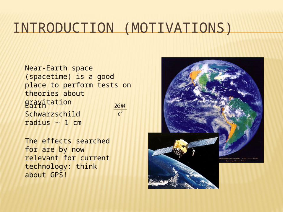
Near-Earth space (spacetime) is a good place to perform tests on theories about gravitation
Earth Schwarzschild radius 1 cm
The effects searched for are by now relevant for current technology: think about GPS!
2
2
c
GM

INTRODUCTION (MOTIVATIONS)
What do we need in order to perform good science?
A theory: Schwarzschild, Kerr (gravitomagnetism) exact solutions sufficiently general to be descriptive and predictive
Contat points with experiment: weak field and slow motion, PPN formalism
A probe: test masses

LAGEOS SATELLITES AND SLR
LAGEOS AND SLR
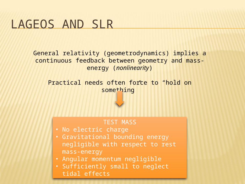
General relativity (geometrodynamics) implies a continuous feedback between geometry and mass-energy
(nonlinearity)
Practical needs often force to “hold on something”
TEST MASS• No electric charge• Gravitational bounding energy
negligible with respect to rest mass-energy
• Angular momentum negligible• Sufficiently small to neglect tidal
effects

THE MOONThe smallness of a test mass depends on the scale under consideration
LAGEOS and SLR
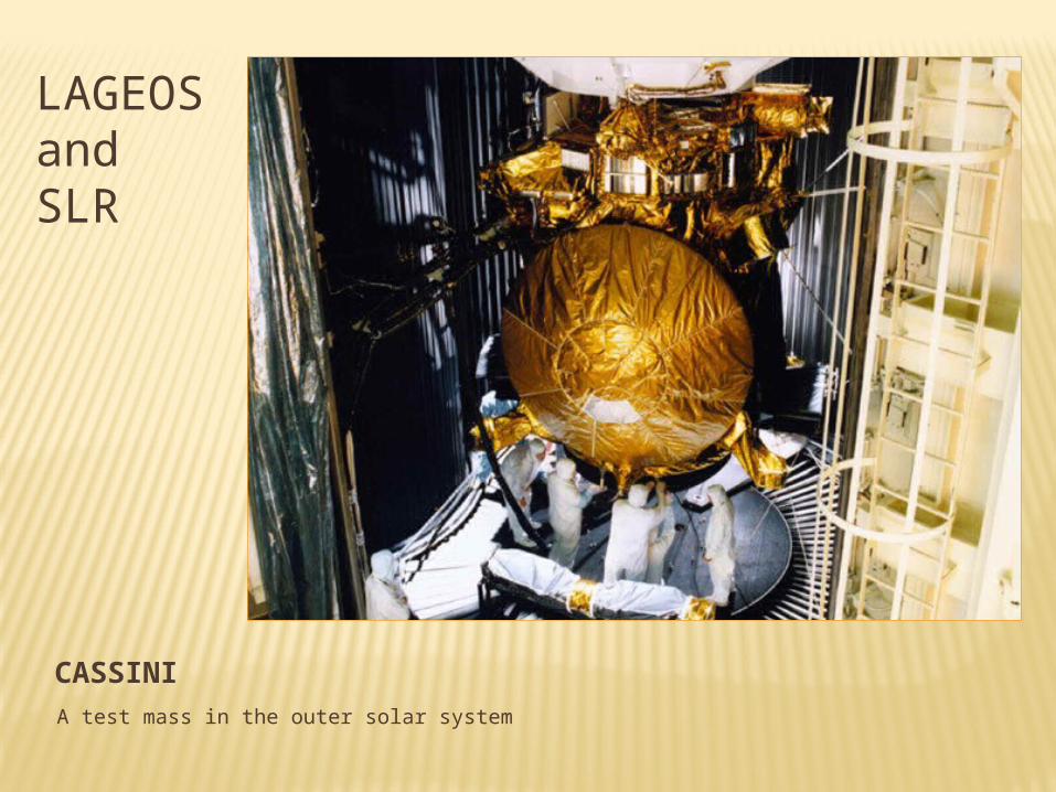
CASSINIA test mass in the outer solar system
LAGEOS and SLR

BEPICOLOMBOA future test mass pretty close to the Sun
LAGEOS and SLR

LAGEOS IIThe LAGEOS satellite are probably the closest to the ideal concept of a test mass
LAGEOS and SLR
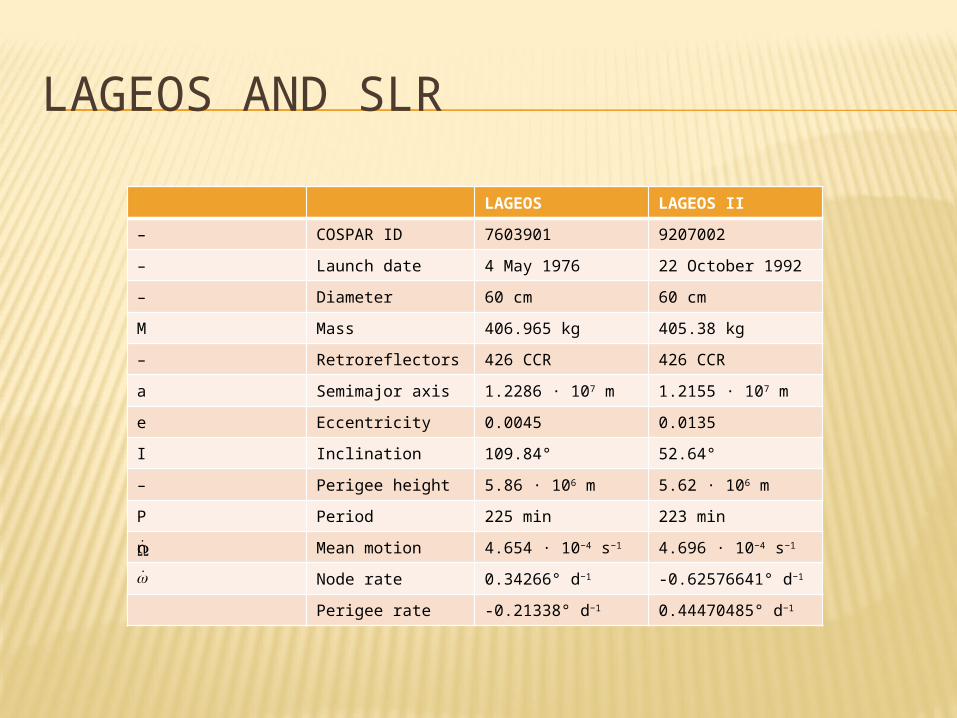
LAGEOS AND SLR
LAGEOS LAGEOS II
– COSPAR ID 7603901 9207002
– Launch date 4 May 1976 22 October 1992
– Diameter 60 cm 60 cm
M Mass 406.965 kg 405.38 kg
– Retroreflectors 426 CCR 426 CCR
a Semimajor axis 1.2286 · 107 m 1.2155 · 107 m
e Eccentricity 0.0045 0.0135
I Inclination 109.84° 52.64°
– Perigee height 5.86 · 106 m 5.62 · 106 m
P Period 225 min 223 min
n Mean motion 4.654 · 10−4 s−1 4.696 · 10−4 s−1
Node rate 0.34266° d−1 -0.62576641° d−1
Perigee rate -0.21338° d−1 0.44470485° d−1

LAGEOS AND SLR
Satellite Laser Ranging (SLR)A laser pulse from a ground station is sent to the satellite, where it is reflected back in the same direction from optical elements called Cube Corner Retroreflectors (CCR)The precision of this technique is noteworthy ( 1 mm)
Matera MLRO
CCRilrs.gsfc.nasa.gov

INTERNATIONAL LASER RANGING SERVICE (ILRS) NETWORK
ilrs.gsfc.nasa.gov
LAGEOS and SLR
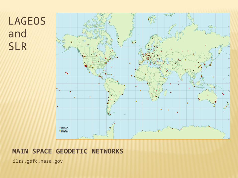
MAIN SPACE GEODETIC NETWORKSilrs.gsfc.nasa.gov
LAGEOS and SLR
GRAVITOMAGNETISM (IN WEAK-FIELD AND SLOW-MOTION)
GRAVITOMAGNETISM
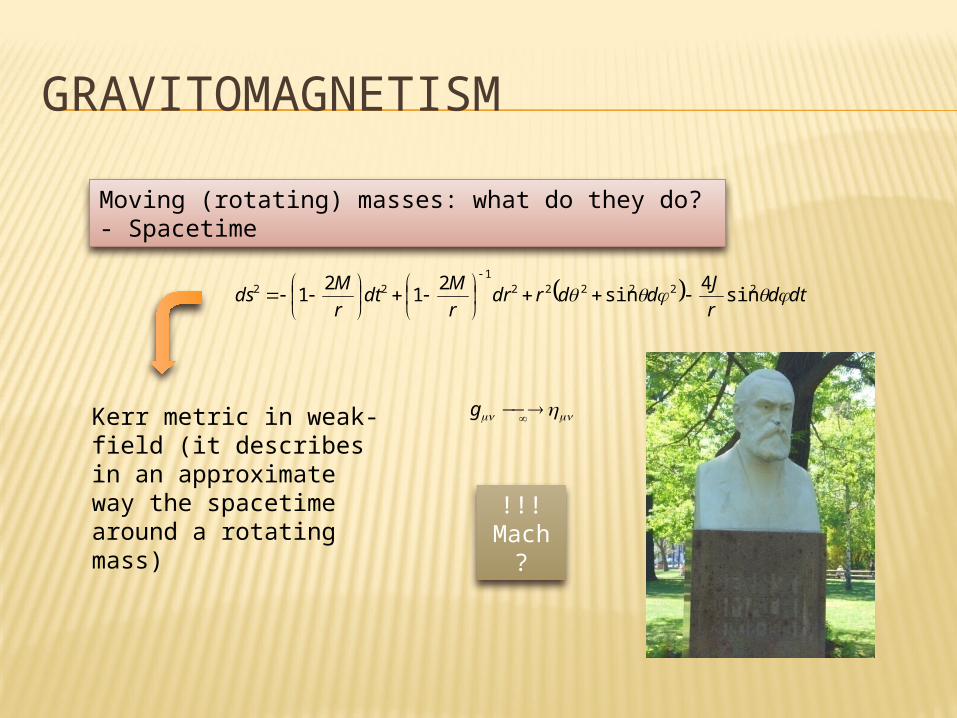
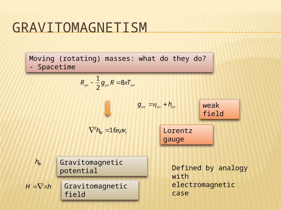
Moving (rotating) masses: what do they do? - Spacetime
dtdr
Jddrdr
r
Mdt
r
Mds 222222
122 sin
4sin
21
21
Kerr metric in weak-field (it describes in an approximate way the spacetime around a rotating mass)
g
!!!Mach
?
GRAVITOMAGNETISM
Moving (rotating) masses: what do they do? - Spacetime
TRgR 82
1
hg
ii vh 1602
weak field
Lorentz gauge
hH
ih0 Gravitomagnetic potential
Gravitomagnetic field
Defined by analogy with electromagnetic case
GRAVITOMAGNETISM
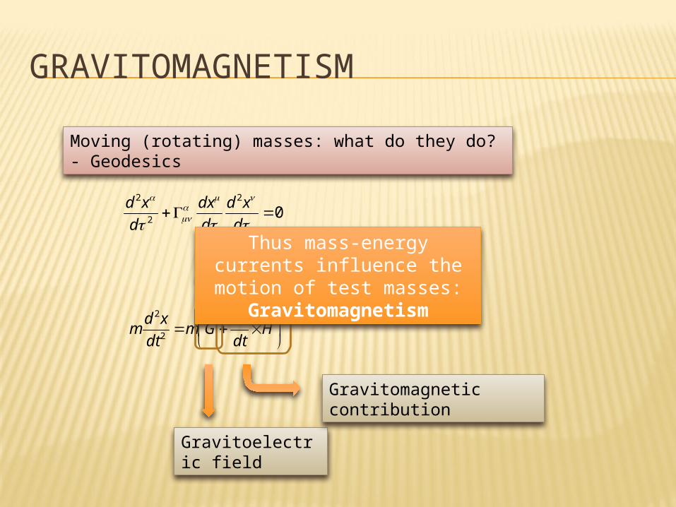
Moving (rotating) masses: what do they do? - Geodesics
02
2
2
d
xd
d
dx
d
xd
Slow-motion
H
dt
xdGm
dt
xdm
2
2
Gravitoelectric field
Gravitomagnetic contribution
Thus mass-energy currents influence the motion of test
masses:Gravitomagnetism

GRAVITOMAGNETISM
32)(x
xJxh
3
ˆ)ˆ(32
x
xxJJH
3
ˆ)ˆ(3
x
xxJJ
Spherically symmetric rotating mass-energy distribution (J is the angular momentum associated to the distribution)
A gyroscope in a gravitomagnetic field precesses
Dragging of inertial frames

GRAVITOMAGNETISM
Obtain a solution
Celestial mechanics tools
• Osculating ellipse (Keplerian elements)• Perturbation first-order analysis (Lagrange and
Gauss equations)
• Periodic effects• Secular effects (
t)
GRAVITOMAGNETISM
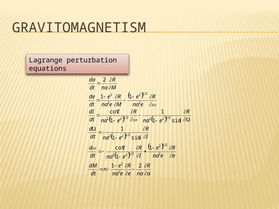
Lagrange perturbation equations
a
R
nae
R
ena
en
dt
dM
e
R
ena
e
I
R
ena
I
dt
d
I
R
Ienadt
d
R
Iena
R
ena
I
dt
dI
R
ena
e
M
R
ena
e
dt
de
M
R
nadt
da
21
1
1
cot
sin1
1
sin1
1
1
cot
11
2
2
2
2
2/12
2/122
2/122
2/1222/122
2
2/12
2
2
GRAVITOMAGNETISM
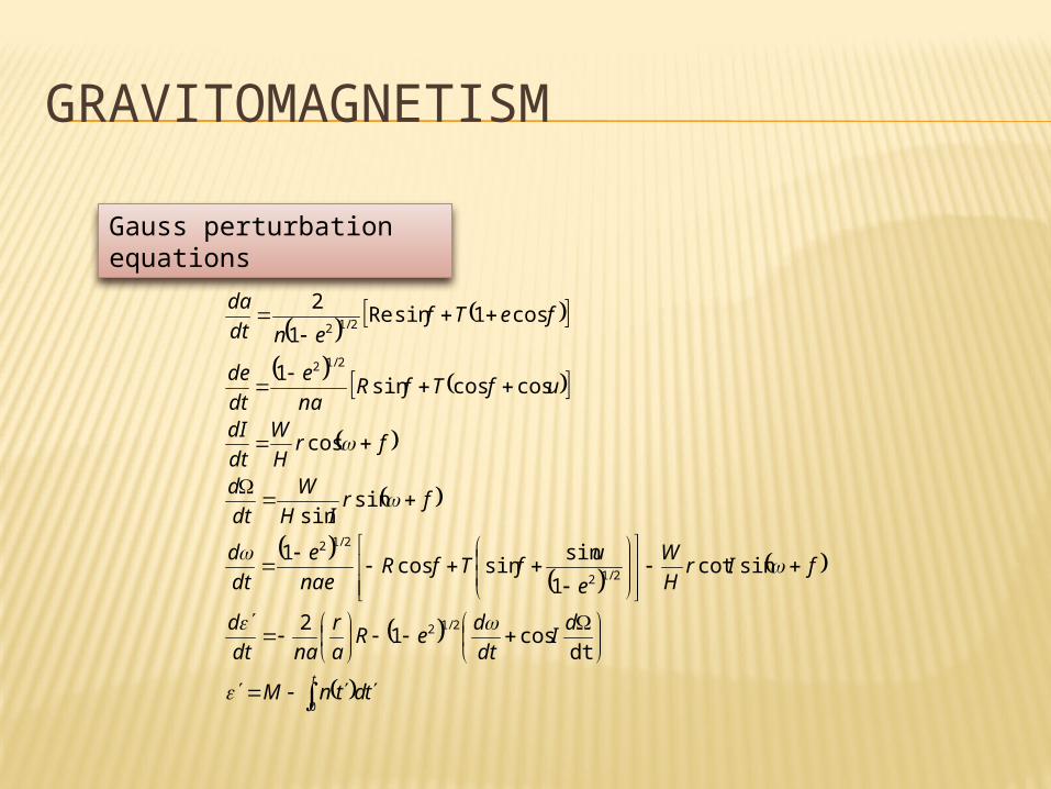
Gauss perturbation equations
ttdtnM
dI
dt
deR
a
r
nadt
d
fIrH
W
e
ufTfR
nae
e
dt
d
frIH
W
dt
d
frH
W
dt
dI
ufTfRna
e
dt
de
feTfendt
da
0
2/12
2/12
2/12
2/12
2/12
dtcos1
2
sincot1
sinsincos
1
sinsin
cos
coscossin1
cos1sinRe1
2
GRAVITOMAGNETISM
2/3232 1
2
eac
GJTL
Ieac
GJTL cos1
62/3232
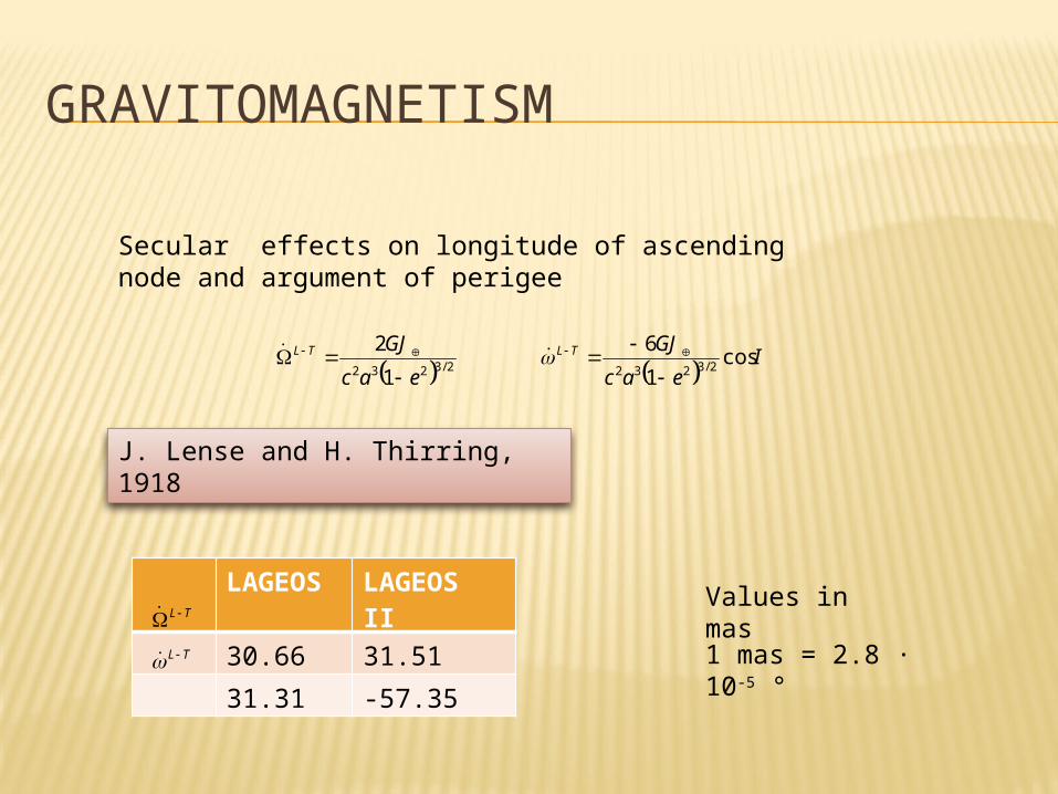
Secular effects on longitude of ascending node and argument of perigee
J. Lense and H. Thirring, 1918
LAGEOS
LAGEOS II
30.66 31.51
31.31 -57.35
Values in mas1 mas = 2.8 ∙ 10-5 °
TL
TL

PARAMETER ESTIMATION

W
P
CM
COf
dPz
j
iij
iii
ii
PARAMETER ESTIMATION
Differential correction procedure
j ij
j
iii dOdP
P
CCO
fWMMWMz TT 111
Corrections to the models parameters
Residuals
Observation equations
Least-squares (normal equations)
Partials
Covariance matrix
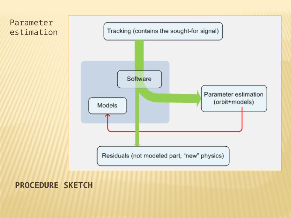
PROCEDURE SKETCH
Parameter estimation
MODELS
MODELS
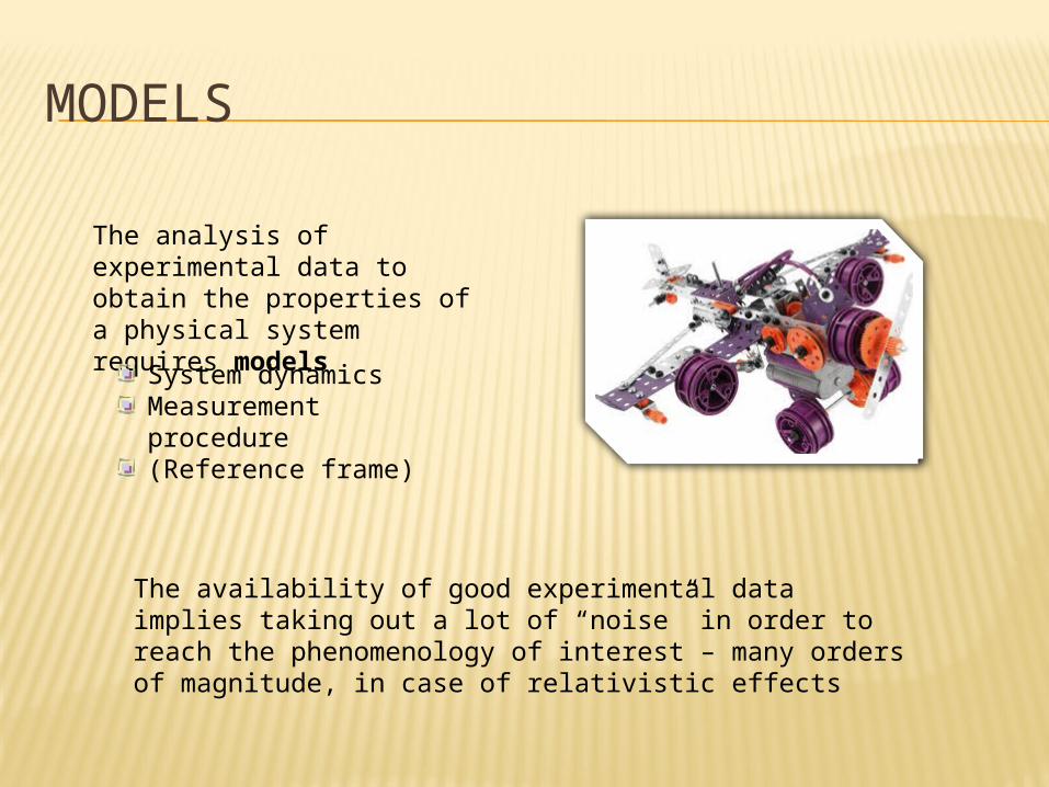
The analysis of experimental data to obtain the properties of a physical system requires models
System dynamicsMeasurement procedure(Reference frame)
The availability of good experimental data implies taking out a lot of “noise” in order to reach the phenomenology of interest – many orders of magnitude, in case of relativistic effects

MODELS
• Geopotential (static part)• Solid Earth and ocean tides / Other temporal
variations of geopotential• Third body (Sun, Moon and planets)• de Sitter precession• Deviations from geodetic motion• Other relativistic effects• Direct solar radiation pressure• Earth albedo radiation pressure• Anisotropic emission of thermal radiation due to
visible solar radiation (Yarkovsky-Schach effect)• Anisotropic emission of thermal radiation due to
infrared Earth radiation (Yarkovsky-Rubincam effect)
• Asymmetric reflectivity• Neutral and charged particle drag
Gravitational
Non-gravitational

MODELS
Cause Formula Acceleration (m s-2)
Earth’s monopole 2.8
Earth’s oblateness 1.0 ∙ 10-3
Low-order geopotential harmonics
6.0 ∙ 10-6
High-order geopotential harmonics
6.9 ∙ 10-12
Perturbation due to the Moon
2.1 ∙ 10-6
Perturbation due to the Sun
9.6 ∙ 10-7
General relativistic correction
9.5 ∙ 10-10
Table taken from A. Milani, A. Nobili, and P. Farinella, Non–gravitational perturbations and satellite geodesy, Adam Hilger, 1987
2r
GM
20
2
23 J
r
R
r
GM
224
2
3 Jr
RGM
18,1820
18
19 Jr
RGM
rr
GM
Moon
Moon3
2
rr
GM
Sun
Sun3
2
rc
GM
r
GM 122

MODELS
Cause Formula Acceleration (m s-2)
Atmospheric drag 3 ∙ 10-12
Solar radiation pressure
3.2 ∙ 10-9
Earth’s albedo radiation pressure
3.4 ∙ 10-10
Thermal emission 1.9 ∙ 10-12
Dynamic solid tide 3.7 ∙ 10-8
Dynamic ocean tide 0.1 of the dynamic solid tide
3.7 ∙ 10-9
Reference system: non-rigid Earth nutation (fortnightly term)
0.002 arsec in 14 days
3.5 ∙ 10-12
Table taken from A. Milani, A. Nobili, and P. Farinella, Non–gravitational perturbations and satellite geodesy, Adam Hilger, 1987
2
2
1V
M
ACD
cM
A Sun
2
r
RA
cM
A Sun
09
4
T
T
cM
A Sun
4
32
23 r
R
r
R
r
GMk
MoonMoon
Moon
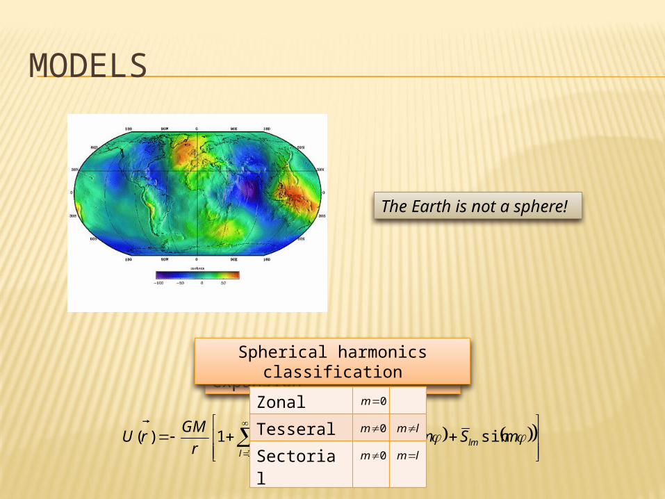
MODELS
The Earth is not a sphere!
Spherical harmonics expansion
1 0
sincoscos1)(l
l
mlmlmlm
l
mSmCPr
R
r
GMrU
Spherical harmonics classification
Zonal
Tesseral
Sectorial
0m
0m
lm
lm
0m

MODELS
Quadrupole perturbation (l = 2, m = 0) to first order
2/32
22
20
22
22
20
22
2
20
1
cos31
4
3
1
cos51
4
3
1
cos
2
3
0
0
0
e
I
a
RnCn
dt
dM
e
I
a
RnC
dt
d
e
I
a
RnC
dt
d
dt
dIdt
dedt
da
MODELS
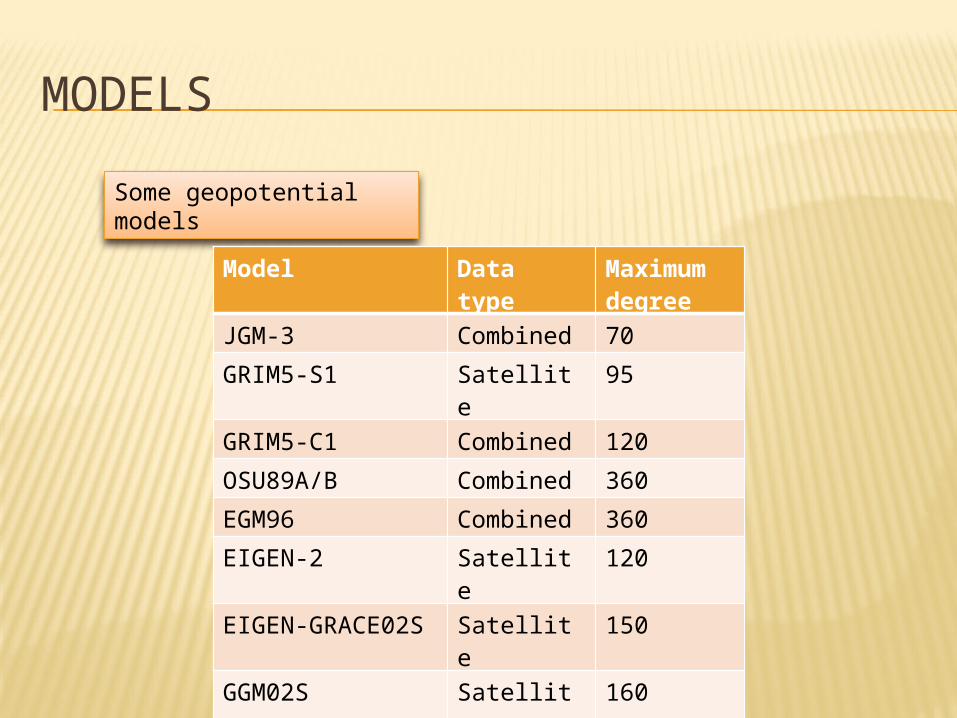
Some geopotential models
Model Data type
Maximum degree
JGM-3 Combined 70
GRIM5-S1 Satellite 95
GRIM5-C1 Combined 120
OSU89A/B Combined 360
EGM96 Combined 360
EIGEN-2 Satellite 120
EIGEN-GRACE02S Satellite 150
GGM02S Satellite 160
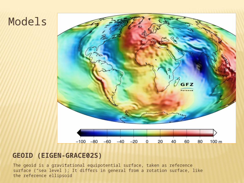
GEOID (EIGEN-GRACE02S)The geoid is a gravitational equipotential surface, taken as reference surface (“sea level”); It differs in general from a rotation surface, like the reference ellipsoid
Models

GRAVITY ANOMALIES (EIGEN-GRACE02S)The gravity anomalies are the difference between the real gravity field and that of a reference body (rotation ellipsoid)
Models
MODELS
l
mlmlml SC
lC
0
222
12
1
4
102 10
7.0l
Cl
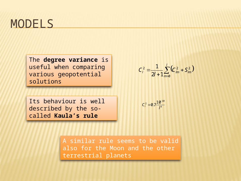
The degree variance is useful when comparing various geopotential solutions
Its behaviour is well described by the so-called Kaula’s rule
A similar rule seems to be valid also for the Moon and the other terrestrial planets

EGM96 AND KAULA’S RULEEarth geopotential degree variance is well approximated by Kaula’s rule
Models
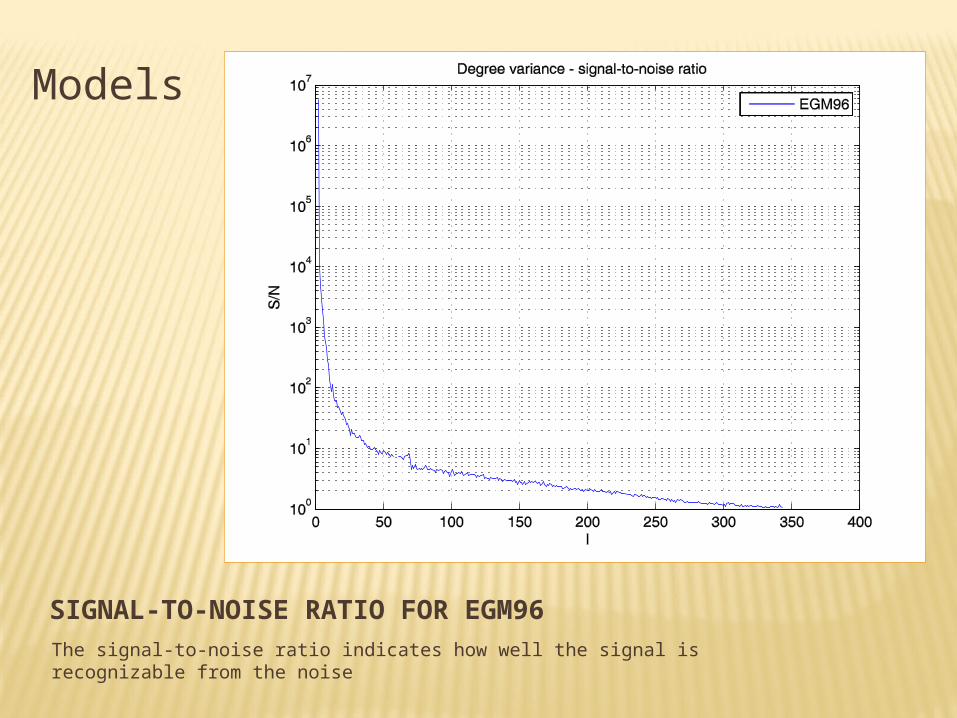
SIGNAL-TO-NOISE RATIO FOR EGM96The signal-to-noise ratio indicates how well the signal is recognizable from the noise
Models
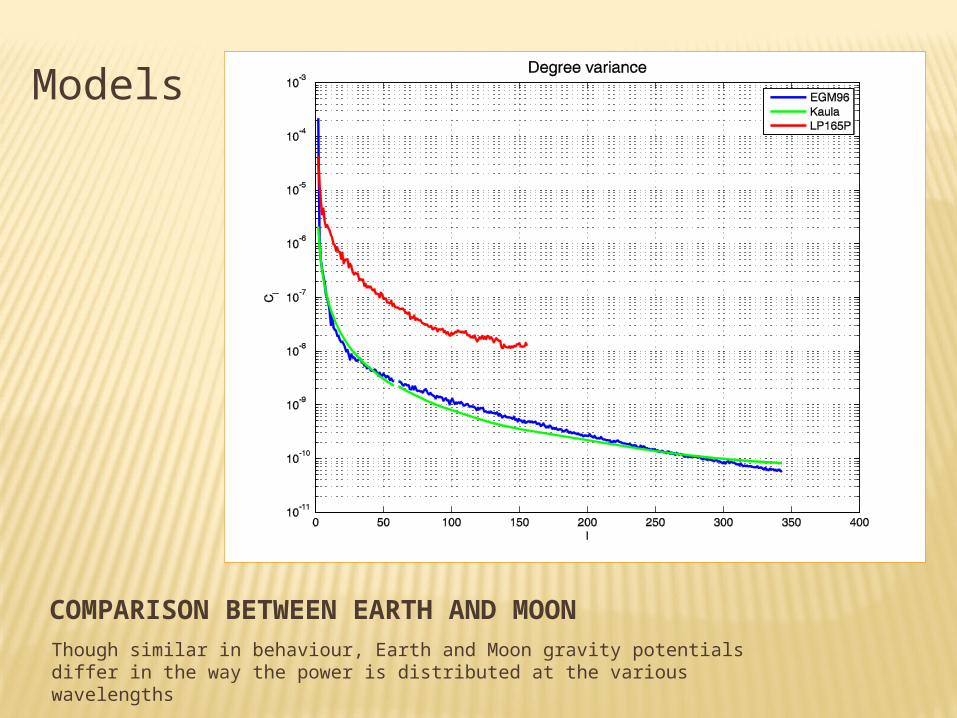
COMPARISON BETWEEN EARTH AND MOONThough similar in behaviour, Earth and Moon gravity potentials differ in the way the power is distributed at the various wavelengths
Models
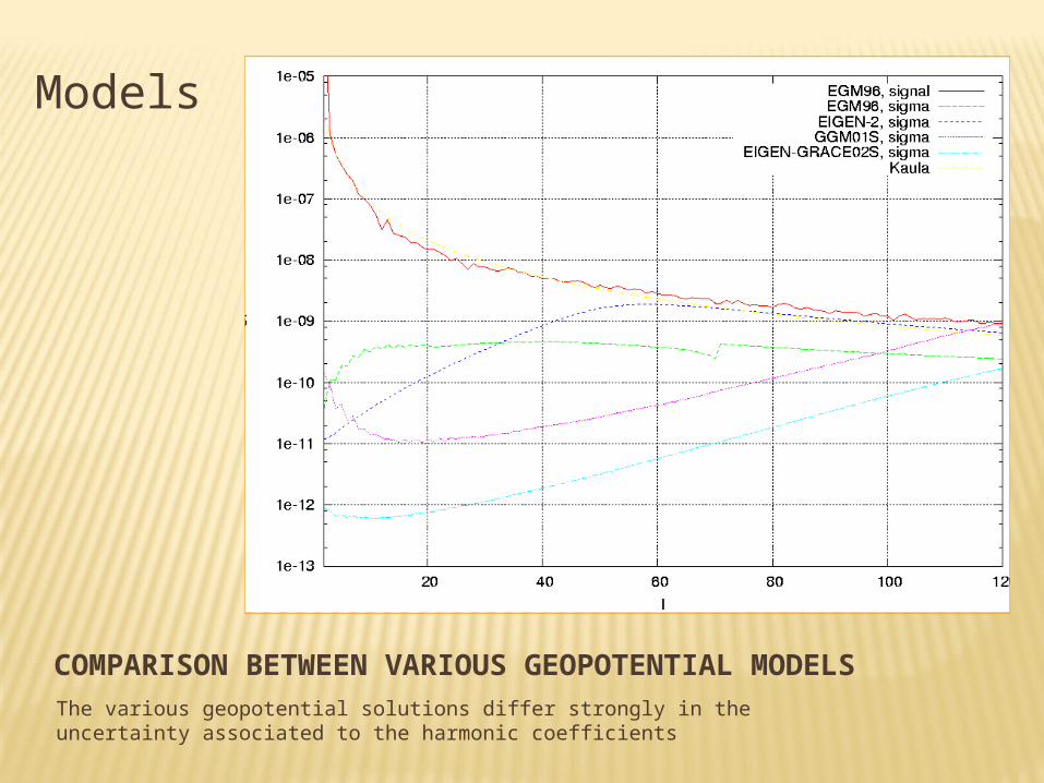
COMPARISON BETWEEN VARIOUS GEOPOTENTIAL MODELS
The various geopotential solutions differ strongly in the uncertainty associated to the harmonic coefficients
Models
MODELS
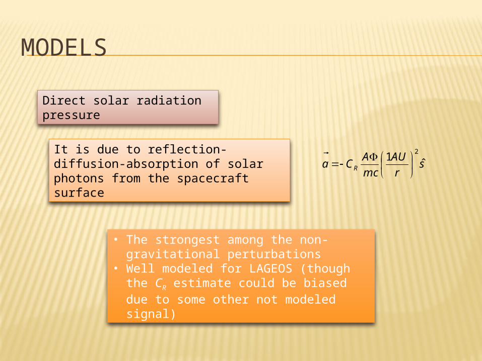
Direct solar radiation pressure
It is due to reflection-diffusion-absorption of solar photons from the spacecraft surface
sr
AU
mc
ACa R ˆ
12
• The strongest among the non-gravitational perturbations
• Well modeled for LAGEOS (though the CR estimate could be biased due to some other not modeled signal)
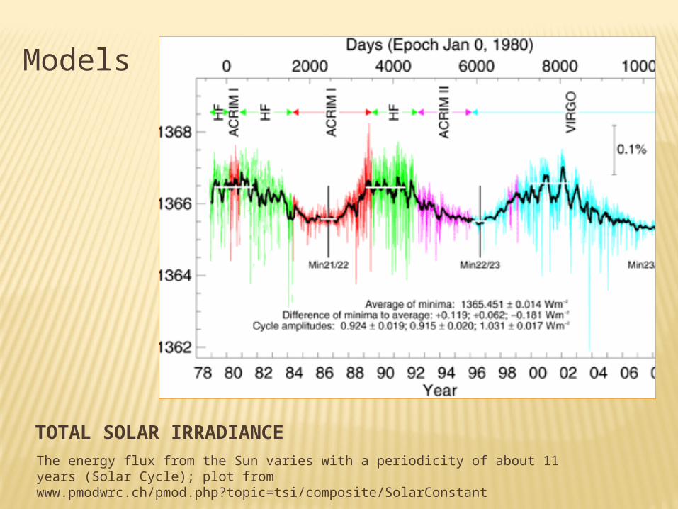
TOTAL SOLAR IRRADIANCEThe energy flux from the Sun varies with a periodicity of about 11 years (Solar Cycle); plot from www.pmodwrc.ch/pmod.php?topic=tsi/composite/SolarConstant
Models

MODELS
Yarkovsky-Schach effect
It is due to infrared radiation anisotropically emitted from the satellite (warmed by the Sun)
SaYar ˆcos
TTRmcir 3
02
9
16
• Effective on argument of perigee behaviour• Difficult modelization (the acceleration depends
on S)
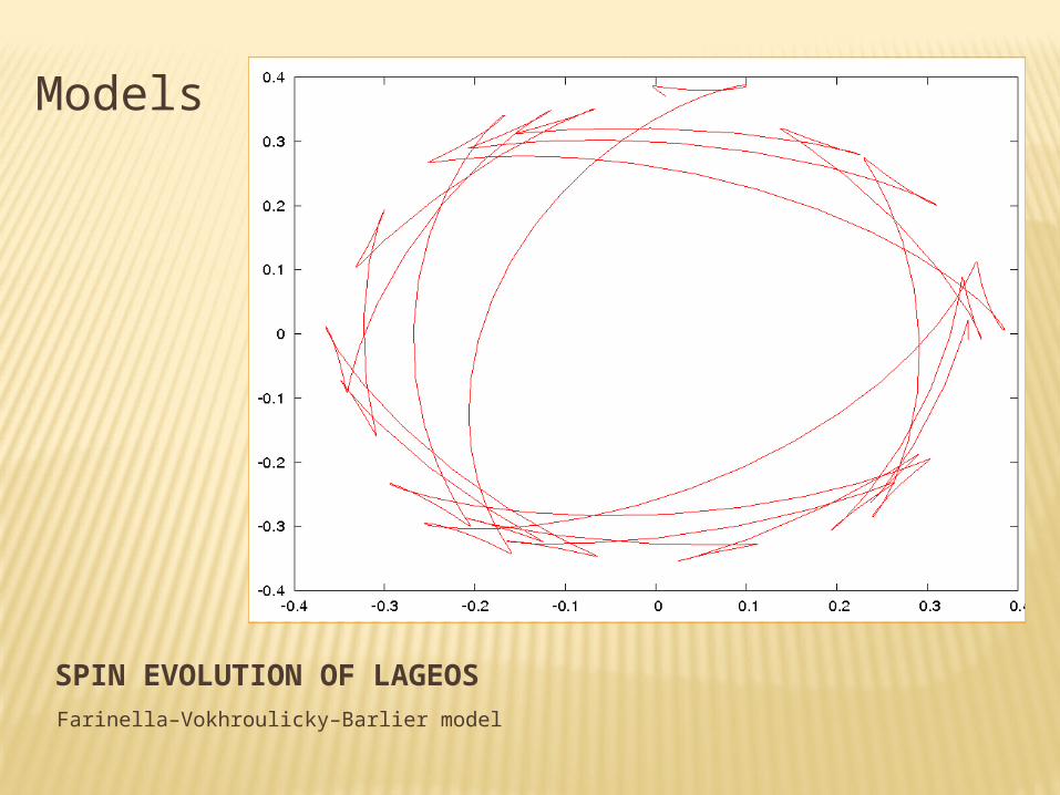
SPIN EVOLUTION OF LAGEOSFarinella–Vokhroulicky–Barlier model
Models
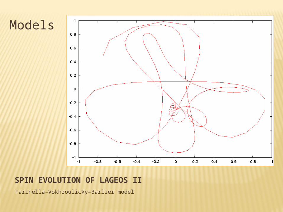
SPIN EVOLUTION OF LAGEOS IIFarinella–Vokhroulicky–Barlier model
Models

MODELS
“Inertial” reference
frame
ICRF
Precession
Nutation
Length of Day
Pole motion
ITRF
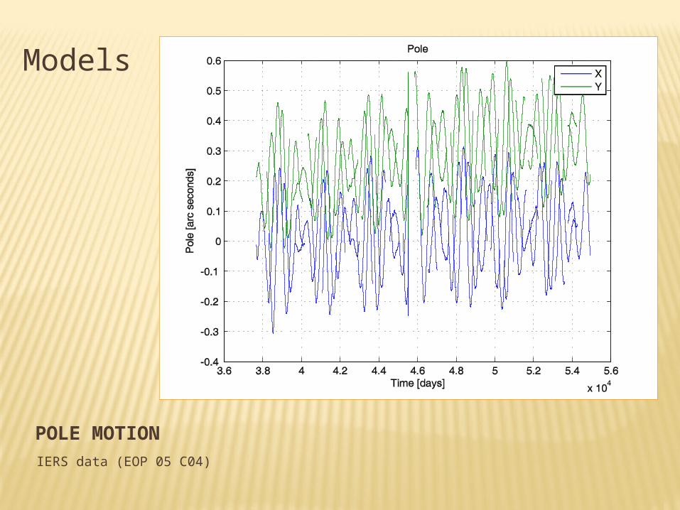
POLE MOTIONIERS data (EOP 05 C04)
Models

LENGTH OF DAY VARIATIONIERS data (EOP 05 C04)
Models
DATA ANALYSIS (EXTRACTING PHYSICS)

DATA ANALYSIS
• Tracking data: Normal Point from ILRS• Software: Geodyn II (NASA GSFC)• Arc length: 15 days• Estimate: state vector and other model
parameters• Further information: residuals
RESIDUAL = OBSERVED - CALCULATED
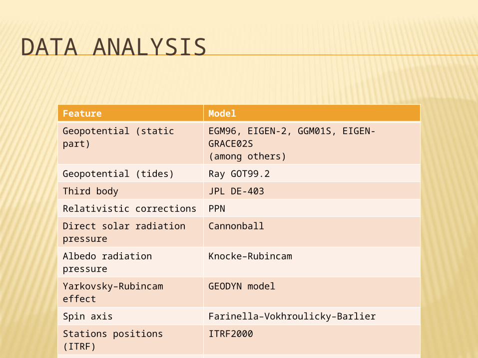
DATA ANALYSIS
Feature Model
Geopotential (static part) EGM96, EIGEN-2, GGM01S, EIGEN-GRACE02S(among others)
Geopotential (tides) Ray GOT99.2
Third body JPL DE-403
Relativistic corrections PPN
Direct solar radiation pressure
Cannonball
Albedo radiation pressure Knocke–Rubincam
Yarkovsky–Rubincam effect GEODYN model
Spin axis Farinella–Vokhroulicky–Barlier
Stations positions (ITRF) ITRF2000
Ocean load Scherneck with GOT99.2 tides
Pole motion IERS EOP
Earth rotation IERS EOP
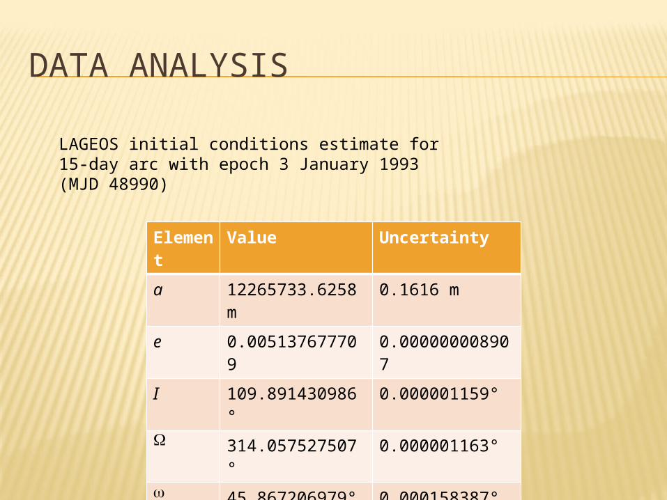
DATA ANALYSIS
Element
Value Uncertainty
a 12265733.6258 m
0.1616 m
e 0.005137677709
0.000000008907
I 109.891430986°
0.000001159°
314.057527507°
0.000001163°
45.867206979° 0.000158387°
M 212.542258784°
0.000157151°
LAGEOS initial conditions estimate for 15-day arc with epoch 3 January 1993 (MJD 48990)
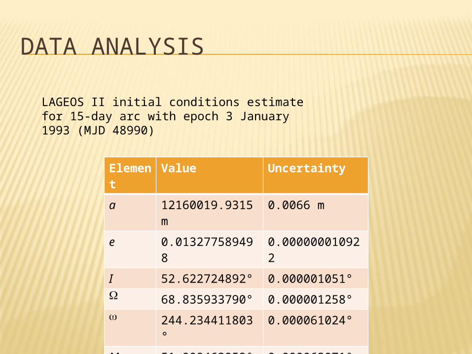
DATA ANALYSIS
Element
Value Uncertainty
a 12160019.9315 m
0.0066 m
e 0.013277589498
0.000000010922
I 52.622724892° 0.000001051° 68.835933790° 0.000001258° 244.234411803
°0.000061024°
M 51.909462952° 0.000063071°
LAGEOS II initial conditions estimate for 15-day arc with epoch 3 January 1993 (MJD 48990)

LAGEOS POST-FIT RMS (EGM96)
Data analysis

LAGEOS II POST-FIT RMS (EGM96)
Data analysis

LAGEOS POST-FIT RMS (VARIOUS MODELS)
Data analysis
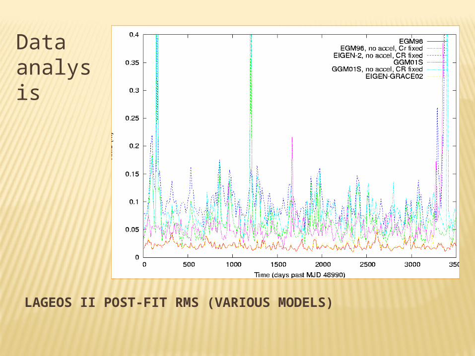
LAGEOS II POST-FIT RMS (VARIOUS MODELS)
Data analysis

Data analysis – Residuals
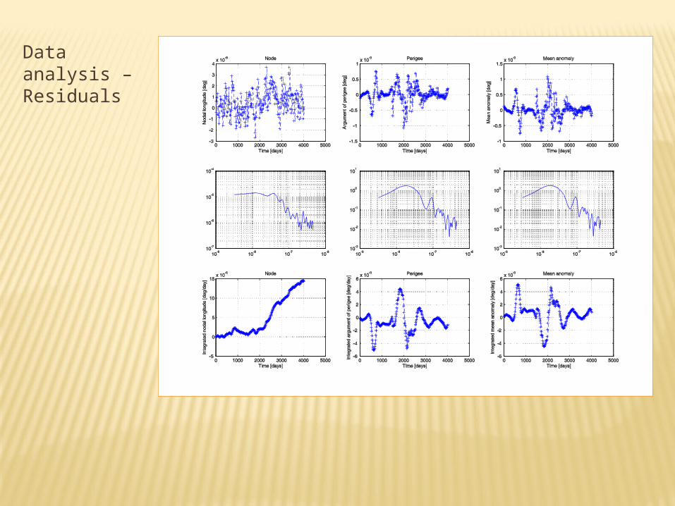
Data analysis – Residuals

DATA ANALYSIS – LENSE-THIRRING
IIII
I
ITL
IIII
ITL
I N
N
N
N
2
2
2
2
The recent geopotential models make critical in the error budget only the uncertainty associated with C20 (Earth quadrupole)
Two-node combination to overcome this problem

SECULAR TREND IN THE COMBINED INTEGRATED NODAL RESIDUALS: EIGEN-GRACE02SCiufolini, Pavlis and Peron, New Astron. 11, 527 (2006)
Data analysis – Lense-Thirring

SECULAR TREND IN THE COMBINED INTEGRATED NODAL RESIDUALS: VARIOUS MODELSA peculiar error estimate is associated to each analysis
Data analysis – Lense-Thirring
DATA ANALYSIS – ESTIMATION BIASES
In common practice often empirical accelerations are included in the modelization setup to take into account small not modeled perturbations
Fit improving Estimation biases risk
Constant part ∼ 10−12 m/s2
Possible correlation between CR and empirical accelerations coefficients
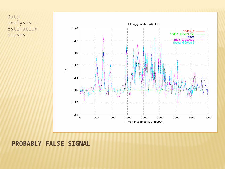
PROBABLY FALSE SIGNAL
Data analysis – Estimation biases

TRUE SIGNAL?Lucchesi et al., Plan. Space Sci. 52, 699 (2004)
Data analysis – Estimation biases
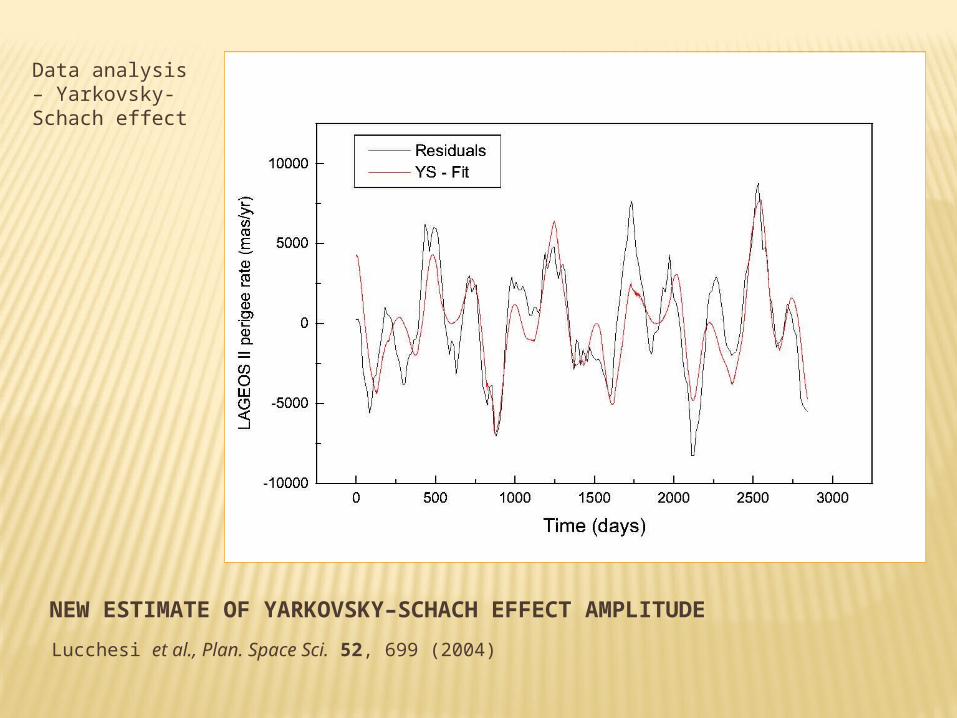
NEW ESTIMATE OF YARKOVSKY–SCHACH EFFECT AMPLITUDE
Lucchesi et al., Plan. Space Sci. 52, 699 (2004)
Data analysis – Yarkovsky-Schach effect

ANOMALOUS NODE RESIDUALS BEHAVIOUR (LAGEOS)
The reported secular trend for the integrated residuals of the longitude of the LAGEOS ascending node abruptly changes from 0.026 mas d−1 to 0.24 mas d−1
Data analysis – Unexpected results

ANOMALOUS NODE RESIDUALS BEHAVIOUR (LAGEOS II)
The reported secular trend for the integrated residuals of the longitude of the LAGEOS II ascending node abruptly changes from -0.0079 mas d−1 to -0.53 mas d−1
Data analysis – Unexpected results
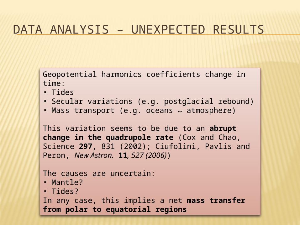
DATA ANALYSIS – UNEXPECTED RESULTS
Geopotential harmonics coefficients change in time:• Tides• Secular variations (e.g. postglacial rebound)• Mass transport (e.g. oceans ↔ atmosphere)
This variation seems to be due to an abrupt change in the quadrupole rate (Cox and Chao, Science 297, 831 (2002); Ciufolini, Pavlis and Peron, New Astron. 11, 527 (2006))
The causes are uncertain:• Mantle?• Tides?In any case, this implies a net mass transfer from polar to equatorial regions

READINGS (MINIMAL SET)
READINGS (MINIMAL SET)
D. W. Sciama, The Unity of the Universe, Faber & Faber, 1959C. W. Misner, K. S. Thorne and J. A. Wheeler, Gravitation, W.H. Freeman and Co., 1973I. Ciufolini and J. A. Wheeler, Gravitation and inertia, Princeton University Press, 1995B. Bertotti, P. Farinella, and D. Vokrouhlický, Physics of the Solar System — Dynamics and Evolution, Space Physics, and Spacetime Structure, Kluwer Academic Publishers, 2003A. Milani, A. Nobili, and P. Farinella, Non–gravitational perturbations and satellite geodesy, Adam Hilger, 1987O. Montenbruck and E. Gill, Satellite Orbits — Models, Methods and Applications, Springer, 2000C. M. Will, The Confrontation between General Relativity and Experiment, Living Rev. Relativity 9, (2006), 3, http://www.livingreviews.org/lrr-2006-3D. McCarthy, and G. Petit (eds.), IERS Conventions (2003), IERS, 2004


