

Rocketsondes/lidars
by P. Keckhut et al.
Talk given by Chantal CLAUD,LMD, Palaiseau, France
+ some other considerations
(EUROSPICE, SOLICE projects)

Rocketsonde and lidar locations and periods of coverage.
Station Reference Latitude Period Instrument
Low latitude stations Keckhut et al. [1998] From 8°S to 34°N 1969-1992 US rocketsondeRyori, Japan Keckhut and Kodera [1999] 39°N 1969-1996 Japan rocketsondeOHP, France Ramaswamy et al. [2001] 44°N 1979-2001 French lidar
Volgograd, Russia This study 48.68°N 1969-1995 USSR rocketsondeWallops Island, Virginia Schmidlin et al. [1998] 37.5°N 1970-1991 US rocketsonde
This study: « Temperature trends in the middle atmosphere of the mid-latitude as seen by systematic rocket launches above Volgograd” Agnès Kubicki1, Philippe Keckhut1*, Marie-Lise Chanin1, Alain Hauchecorne1,Evgeny Lysenko2, Georgy Golitsyn2

Instrumental changes on US Rocket
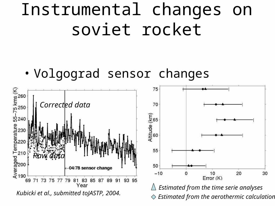
Instrumental changes on soviet rocket
• Volgograd sensor changes
Estimated from the time serie analyses
Estimated from the aerothermic calculations
Raw data
Corrected data
Kubicki et al., submitted toJASTP, 2004.

Tidal interferences
They induce large interferences in data comparisons, trends and satellite validations
6K
Keckhut et al., J. Geophys. Res., p10299, 1996
Keckhut et al., J. Geophys. Res., p447, 1999

Tidal interferences
• Volgograd
Time of launch Averaged temperature 45-55 km
2:00
10:0015:00
Kubicki et al., submitted toJASTP , 2004.
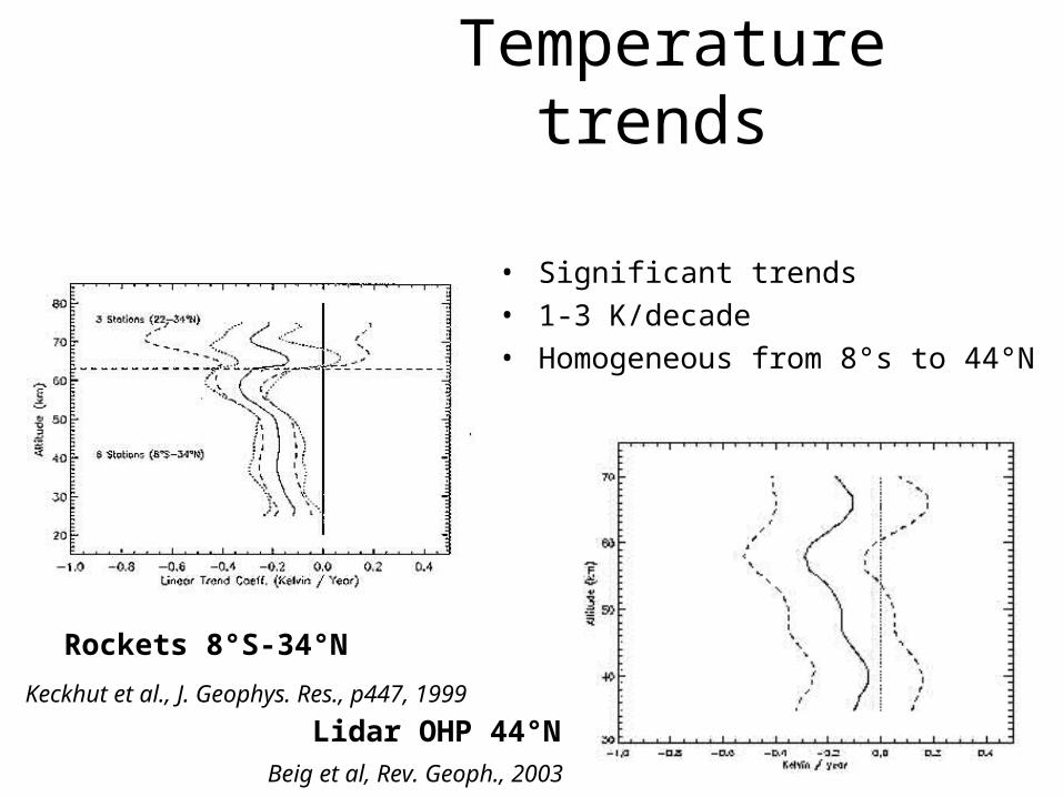
Temperature trends
Rockets 8°S-34°N
Lidar OHP 44°N
• Significant trends
• 1-3 K/decade
• Homogeneous from 8°s to 44°N
Keckhut et al., J. Geophys. Res., p447, 1999
Beig et al, Rev. Geoph., 2003
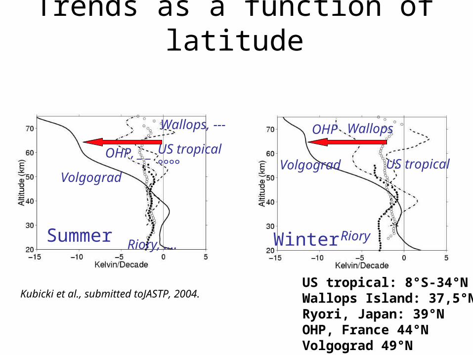
Trends as a function of latitude
Volgograd
OHP, _ _
Wallops, ---
Riory, ….
US tropical°°°° US tropical
WallopsOHP
Volgograd
RiorySummer Winter
Kubicki et al., submitted toJASTP, 2004.US tropical: 8°S-34°NWallops Island: 37,5°NRyori, Japan: 39°NOHP, France 44°NVolgograd 49°N
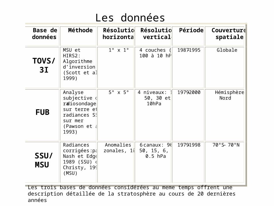
Les donnéesBase de données
Méthode Résolution horizontale
Résolution verticale
Période Couverture spatiale
TOVS/
3I
MSU et HIRS2 : Algorithme d’inversion 3I (Scott et al., 1999)
1° x 1° 4 couches (de 100 à 10 hPa)
1987-1995 Globale
FUB
Analyse subjective de radiosondages sur terre et radiances SSU sur mer (Pawson et al., 1993)
5° x 5° 4 niveaux: 100, 50, 30 et 10hPa
1979-2000
Hémisphère Nord
SSU/ MSU
Radiances corrigées par : Nash et Edge, 1989 (SSU) et Christy, 1993 (MSU)
Anomalies zonales, 10°
6 canaux: 90, 50, 15, 6, 1.5,
0.5 hPa
1979-1998 70°S - 70°N
Les trois bases de données considérées au meme temps offrent une description détaillée de la stratosphère au cours de 20 dernières années
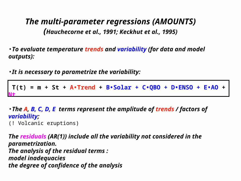
The multi-parameter regressions
(AMOUNTS)(Hauchecorne et al., 1991; Keckhut et al., 1995)
•To evaluate temperature trends and variability (for data and model outputs):
•It is necessary to parametrize the variability:
T(t) = m + St + A•Trend + B•Solar + C•QBO + D•ENSO + E•AO + Nt
•The A, B, C, D, E terms represent the amplitude of trends / factors of variability; (! Volcanic eruptions)
The residuals (AR(1)) include all the variability not considered in the parametrization.The analysis of the residual terms : model inadequacies the degree of confidence of the analysis
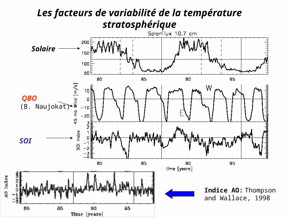
Solaire
SOI
QBO(B. Naujokat)
Indice AO: Thompson and Wallace, 1998
Les facteurs de variabilité de la température stratosphérique
Datasets
• US Rocketsondes 1969-90’s
• LIDAR in France 1970-2001
• SSU 1979-2001
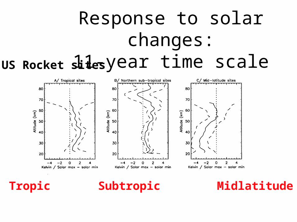
Response to solar changes:11-year time scale
US Rocket sites
Tropic Subtropic Midlatitude
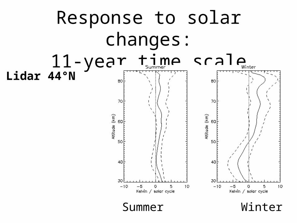
Response to solar changes:11-year time scale
Lidar 44°N
Summer Winter

Response to solar changes:11-year time scale
±60°
SSU at 6 hPa

Response to solar changes
• Photochemical response at low latitude
• Negative response at high latitude• Strong seasonal response
Role of the dynamics?
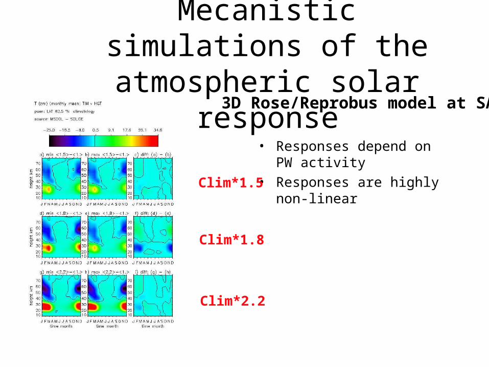
Mecanistic simulations of the atmospheric solar response
• Responses depend on PW activity
• Responses are highly non-linear
Clim*1.5
Clim*1.8
Clim*2.2
3D Rose/Reprobus model at SA

Conclusions
• Equatorial response close to the photochemical response (1-2 K)
• Negative response at mid and high latitude with a strong seasonal effect
• The solar response is strongly related to wave activity • Numerical simulations show a similar response with a
specific planetary wave level

AO regressions
Seasonal regressions at 100 hPa
Vertical structures of annual regressions
Winter
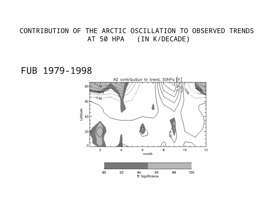
CONTRIBUTION OF THE ARCTIC OSCILLATION TO OBSERVED TRENDS AT 50 HPA (IN K/DECADE)
FUB 1979-1998
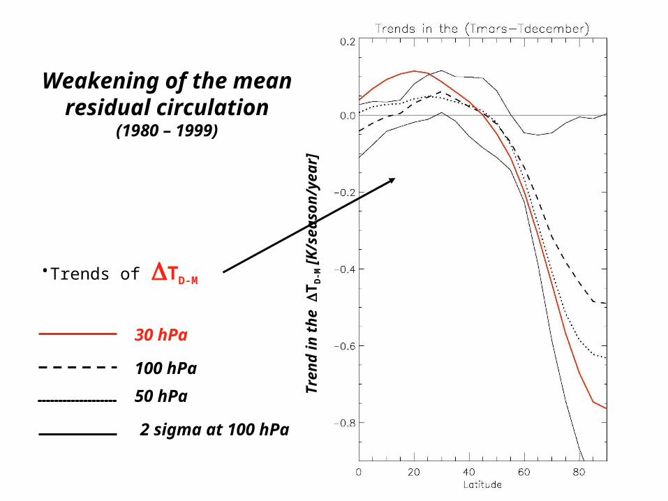
•Trends of TD-M
Weakening of the mean residual
circulation(1980 – 1999)
50 hPa
30 hPa100 hPa
2 sigma at 100 hPa
Tre
nd
in
th
e T
D-M
[K
/season
/year]
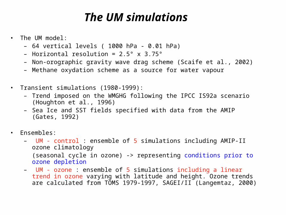
• The UM model:– 64 vertical levels ( 1000 hPa - 0.01 hPa)– Horizontal resolution = 2.5° x 3.75°– Non-orographic gravity wave drag scheme (Scaife et al., 2002)– Methane oxydation scheme as a source for water vapour
• Transient simulations (1980-1999):– Trend imposed on the WMGHG following the IPCC IS92a scenario
(Houghton et al., 1996) – Sea Ice and SST fields specified with data from the AMIP (Gates,
1992)
• Ensembles:– UM - control : ensemble of 5 simulations including AMIP-II ozone
climatology (seasonal cycle in ozone) -> representing conditions prior to ozone depletion
– UM - ozone : ensemble of 5 simulations including a linear trend in ozone varying with latitude and height. Ozone trends are calculated from TOMS 1979-1997, SAGEI/II (Langemtaz, 2000)
The UM simulations
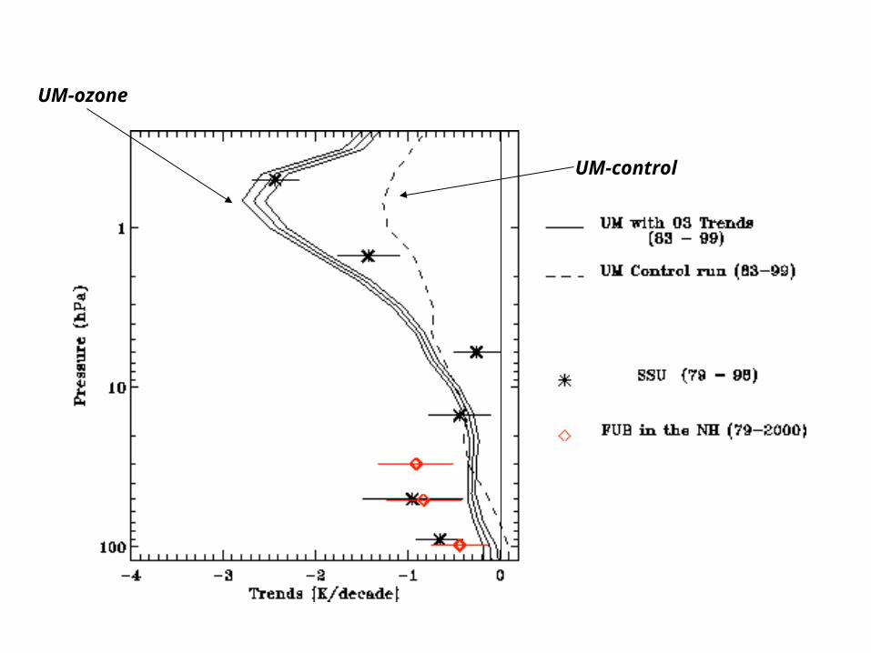
UM-control
UM-ozone
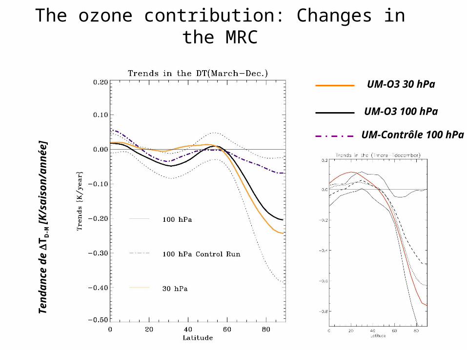
The ozone contribution: Changes in the MRCTen
dan
ce d
e
TD
-M [
K/s
ais
on
/an
née]
UM-O3 30 hPa
UM-O3 100 hPa
UM-Contrôle 100 hPa

Fz trends (Jan- Feb- March)
Ozone changes responsible for reduction in wave activity in high latitudes during late winter? Proposed mechanism: (Hu et Tung, 2003)
UM-ozone
UM-control
Concerning the future…
Russian rockets data continue after 1995, negociations to acquire them also…Lidar data from TMF (Table Mountain Facility, California) whichcover the period 1988-present might be useful. Other lidars data begin after 1995, so that the record might be too short.
At SA, Agnes Kubicki will work on Heiss (82°N), Molodesnaya (67°S), and Thumba (8°N) records.From May 2005 on, Serge Guillas will work on non-linear methodsto determine trends (bootstrap).At LMD, work will continue on trend determination (FUB). At SA and LMD, a 20 years run from LMDz-Reprobus is available.


