
I
384021
Standardization of Asphalt Viscosity and Mix Design Procedures
EGONS TONS
Professor of Civil Engineering
ROBERT 0. GOETZ
Associate Professor of Civil Engineering
and
RICHARD MOORE
Research Assistant
MICHIGAN DEPARTMENT OF
June 1975 TRANSPORTATION liBRARY LANSING ·---- ·-- 48909
Michigan Department of State Highways and Transportation Contract No. 74-0792 Lansing, Michigan
Department of Civil Engineering
T H E U N I V E R S I T Y 0 F M I C H I G A N
COLLEGE OF ENGINEERING
Department of Civil Engineering
STANDARDIZATION OF ASPHALT VISCOSITY AND MIX DESIGN PROCEDURES
Egons Tons Professor of Civil Engineering
Robert 0. Goetz Associate Professor of Civil Engineering
Richard B. Moore Research Assistant
DRDA Project 384021
under contract with:
MICHIGAN DEPARTMENT OF STATE HIGHWAYS AND TRANSPORTATION CONTRACT NO. 74-0792
LANSING, MICHIGAN
administered through:
DIVISION OF RESEARCH DEVELOPMENT AND ADMINISTRATION THE UNIVERSITY OF MICHIGAN
JUNE 1975
MICHIGAN DEPARTMENT OF
TRANSPORTATION LIBRARY LAi\1SiNG 48909
TABLE OF CONTENTS
Abstrac·t ' . . Acknowledgment
Part A - Viscosity
Grading of Asphalts Used in Michigan by Viscosity at 25 C •• , •. , , . , . , .
Cone-plate viscosity measurement and time
Asphalts used in this investigation . ,
Viscosity - temperature curves for the six sources .. .. " " " .. .. " .. .. "' .. " "'
Development of viscosity grading charts
Establishing the tentative viscosity grading limits , ,
Use of the charts . .
Continued improvement
Further Trials to Simplify the Measurement of Viscosity at 25 C . . • . . . . .
Test apparatus and test procedure
Asphalts used and results .. , .
Part B - Mix Design
Computerized Marshall Mix Design
Basis for design
Data analysis
Advantages of the program
Special precautions .
Further Work on Mix Design Factors
Previous work . . . .
ii
iv
vi
1
2
4
5
6
9
12
13
14
15
16
18
. 18
22
26
27
27
27
Calibration of pouring test apparatus for rugosity determination . . . . .
Comparison of calculated asphalt content with Marshall optimum asphalt content
Conclusions . .
Recommendations
Bibliography
Tables
Figures
Appendices
Appendix A
. . .
Aggregate Parameter Program .••..•.•.•.•
Appendix B Computer Program for Mixture Design Tables
Appendix C Pouring Test and Proposed Standard Apparatus •.•.
Appendix D Corrections to Packing Specific Gravity
Appendix E Selection of Optimum Asphalt Content from Design Tables . . . • . . . . • . . • . . . • . . .
iii
28
34
37
39
41
43
86
143
147
152
160
167
ABSTRACT
STANDARDIZATION OF ASPHALT VISCOSITY AND MIX DESIGN PROCEDURES
By E. Tons, R. 0. Goetz and R. B. Moore The University of Michigan
The main purpose of this work was: (a) to develop
practical procedures for grading asphalt cements by vis-
cosity, and (b) to devise a computerized procedure for bitu-
minous concrete mix design. Both goals were achieved.
Part A of the report describes a method of grading
asphalts used in Michigan by viscosity at 25 C. All together
four viscosity grades are proposed: 150-250, 400-650, 900-
1400 and 1800-2500 kilopoises, replacing the present 200-250,
120-150, 85-100 and 60-70 penetration grades, respectively.
Detailed graphical viscosity charts have been prepared
for six sources (producers) of asphalts which permit producers
to select their asphalts for sale (to the consumer) on the
basis of viscosity at 60 C and 135 C. These charts are ready
to be used for practical application.
At the end of Part A a brief description of a test
using a constant penetration rate is given. More work is
needed to see whether such a test could be used as a simplified
method to measure viscosity at 25 C. The present predicted
iv

number of 18 viscosity tests per day using the cone-plate
viscometer is fair and can be used until a faster test pro
cedure is developed.
Part B of the report describes the development of a
computerized procedure for designing bituminous concrete
mixes. The Marshall method, modified to suit Michigan con
ditions, is used as the basis for the design program. The
method includes both numerical and graphical analyses. This
method has immediate practical application and is already
being used by the Michigan Department of State Highways and
Transportation. The code for the design is MICHMIX. A
similar design package using the Marshall method as described
by The Asphalt Institute is also included in the report
(AIMIX)
The second section of Part B presented in this report
involves further measurements and calculations towards im
provements over the Marshall design, which requires 15 or
more laboratory made specimens for testing to obtain the
answers. Again, more work is needed in this area to make
further improvements. In the meanwhile, the computerized
Marshall method should be useful for practical design pur
poses.
v
ACKNOWLEDGMENT
This research was financed by the Michigan Department
of State Highways and Transportation.
The authors wish to acknowledge the assistance given
by the Michigan Department of State Highways and Transporta
tion Testing Laboratory under the direction of M. E. Witteveen
and P. J. Serafin. Special thanks go to A. P. Chritz,
Assistant Supervising Engineer, Bituminous Technical Services
Unit, Testing Laboratory, Michigan Department of State
Highways and Transportation, who provided technical sug
gestions so that the findings could have more direct prac
tical application. The cooperation of M. A. Etelamaki and
M. E. Simpson of the Michigan Department of State Highways
and Transportation Testing Laboratory is also appreciated.
Part of the experimental work and data analysis per
formed by C. F. Scribner and K. S. Leung, Research Assistants,
The University of Michigan, contributed considerably to this
report. Also, technical assistance rendered by G. J. Dixon,
S. M. Hollister, T. C. Esper and J. E. Lebovic, student
assistants, was very helpful.
vi

DISCLAIMER
The opinions, findings and conclusions expressed in
this publication are those of the authors and not necessarily
those of the Michigan State Highway Commission or The
University of Michigan.
vii
STANDARDIZATION OF ASPHALT VISCOSITY
AND MIX DESIGN PROCEDURES
PART A - VISCOSITY
l. Grading of Asphalts Used in Michigan by Viscosity at 25 C.
The penetration test has served as a useful tool for
grading of asphalts at 25 C for a long time. At present, the
trend is toward use of the fundamental property of viscosity
as a yardstick for classifying the various types of asphalts.
In this change from penetration grading to viscosity grading
of asphalt cements, much discussion has been generated as to
what standard temperature would be best. The temperature at
60 C is presently being used by a number of agencies. This
has shifted the basic control point of asphalt consistency
measurement from 25 C to 60 C, which is well above the average
field temperatures in Northern climates. Therefore, a research
program was undertaken to attempt to develop procedures for
measuring viscosity at temperatures of 25 C and lower (1;2)
This work has indicated that a cone-plate viscometer and
shear rate of -2 -1 2xl0 sec at 25 C can be used for asphalts
supplied to Michigan.
It is recognized that measuring viscosity at 25 C
is more difficult and may be less accurate than at 60 C. Also,
it takes longer to run a viscosity test at 25 C than at 60 c.
This part of the present report describes the further
work in an effort to develop methods ·to grade asphalt cements
l
2
on the basis of viscosity measured at 25 C. A test procedure
for the routine testing of asphalt cements at 25 C is presented.
Further, viscosity measurements at 25·c are correlated with
viscosities measured at 60 C and 135 C. From these correlations,
proposed viscosity grading limits for six asphalt sources in
Michigan have been determined. Using these limits, a series
of twenty-four graphs were constructed for the six sources and
four asphalt grades. The viscosity limits were set for both
original and aged asphalts.
1.1 Cone-plate viscosity measurement and time.
The method of testing for viscosity of asphalt cements
by the cone-plate viscometer can be found in Appendix G of
Reference 1. This method of testing was followed except for
two "improvements":
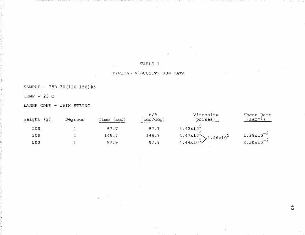
(a) Three weights were used during the test. The
first weight was applied only to find the proper
range of weights to use. In order to calculate
-2 -1 viscosity at a shear rate of 2xl0 sec , one
shear rate had to be below and another above a
certain time (101 to 103.5 seconds, depending
upon the shear rate constant KD) • The second and
third weights were chosen to accommodate this
constraint. From the viscosity and shear values
associated with the two weights, the viscosity
-2 -1 at 2xl0 sec was interpolated. See Table 1
for a typical run.
3
(b) It was also found that asphalts with small samples
to draw from were prone to higher viscosities than
their penetration would indicate, Apparently,
the asphalt "dries out" if there is only a little
of it in the bottom of a sample can. To prevent
this from happening, the sample should be no less
than a full 6 oz. sample can. This is quite
important.
-2 -1 As mentioned before, the shear rate of 2xl0 sec
appears to be "optimum" for Michigan asphalts. If the test is
performed at a higher shear rate, there is a risk (with some
asphalts) of running into so-called non-Newtonian region where
shear stress is no longer proportional to shear rate. On the
other hand, if the shear rate is too slow, it takes a long
time to obtain a viscosity measurement for a given asphalt.
At present, about 50 penetration tests can be made per
day (8 hours) by two operators. A brief study on the number
of viscosity tests possible per 8-hour day (two operators) in-
dicates that 18 readings are possible. To achieve this, four
cone-plate assemblies and two constant temperature baths are
needed. The scheduling for such an operation is given in
Figure l. Although slightly less than half as many samples
can be tested by using the cone-plate viscometer as compared
to regular penetration, this viscosity test procedure appears
to have definite practical promise. Also, the training time
for a technician to run the test is minimal.
4
1.2 Asphalts used in this investigation.
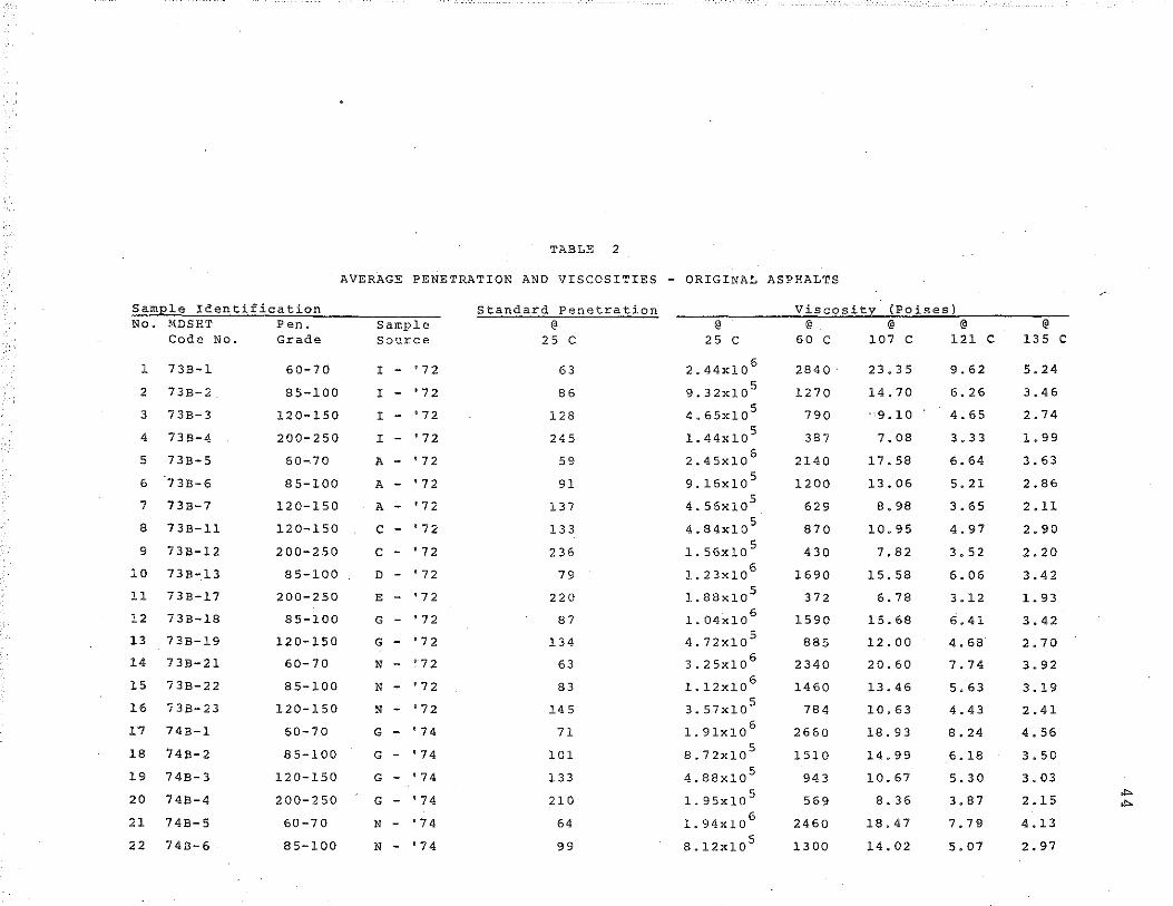
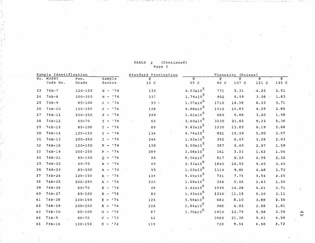
The asphalts used in this investigation were all obtained
from the MDSHT Bituminous Testing Laboratory. These asphalt
samples were collected in 1973, 1974 and 1975 for research and
testing purposes. Data from 73 different asphalts ranging from
high to low penetrations were available for use in this study
and are shown in Table 2. The 1973 and 1974 data have been
reported previously in References 1 and 2. The viscosities
at 135 C have been corrected for the change in specific gravity
of the asphalt with change in temperature. The specific
gravity was used in the conversion from stokes to poises. This
minimal correction was neglected previously. Also shown are
additional viscosity measurements at 107 C (225 F) and 121 C
(250 F). The 1975 data has not been previously reported.
The asphalts presented in Table 2 are labeled as
"original" asphalts to distinguish them from the "aged"
asphalts in Table 3. For the 1975 samples, twenty-eight
asphalts were aged by subjecting them to the thin-film oven test
(ASTM Dl754). The standard penetration and viscosity at various
temperatures were then determined for these samples.
After consultation with MDSHT personnel, six sources
were selected for detailed study in this investigation. These
sources, A-'75, E-'74, G-'74, I-'74, J-'75 and N-'75, furnish
the bulk of the asphalt used in Michigan. Also, they are the
ones for which the most complete data is available. The test
results for these asphalts have been abstracted from Tables 2
and 3 are are presented in Table 4 for ready reference.
1.3 Viscosity - temperature curves for the six sources.
The viscosity data for the six sources is first
presented in a series of viscosity vs. temperature curves,
Figures 2 through 7. These curves are drawn on the ASTM
Standard Viscosity-Temperature Chart for Asphalts (D. 2493).
The solid curves show the relationship for the original
asphalts and the dashed curves for the aged asphalts. Each
curve represents a different asphalt grade.
5
The aged data shown for asphalts A-'75, J-'75 and
N-'75 are the results from the laboratory tests. There were
no aged da·ta for E-'74, G-'74 and I-'74. The aged curves for
these three asphalts were constructed by a method to be dis
cussed later in this section.
Examination of these six figures show that for a given
asphalt grade, viscosi·ty decreases as the temperature increases.
Also, for a given temperature, the viscosity decreases as the
standard penetration increases. Further, for a given asphalt,
the curves for the different grades are nearly parallel. These
relationships are valid for both the original and aged data.
In addition, the aged asphalt curves, for the three sources
where results were available, are close to being parallel to
the original asphalt curves. Apparently, the effect of aging
is to translate the original curves upwards, or in other words,
aging increases the viscosity for a given asphalt.
The apparent parallelism of the viscosity vs. temperature
curves was used to construct aged curves for the three 1974 sources
6
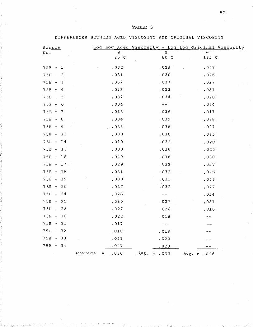
by the following method. The respective differences between the
log log of aged viscosity data (expressed in centipoises) and the
log log of the original viscosity data (centipoises) was
determined for all samples in which aged data was available.
The results are shown in Table 5. For a given temperature,
this difference is fairly consistent and an average value was
computed. At 25 C, the differences ranged from 0.017 to 0.038
with 20 of the 25 samples falling between 0.027 and 0.038.
Comparable figures at 60 C are 0.018 to 0.039 with 17 of 22
ranging from 0.028 to 0.039; and at 135 C, 0.016 to 0.031 with
18 of 20 falling between 0.020 and 0.031. The aged curves
for the three 1974 sources were drawn by adding the average
difference at each temperature to the original viscosities at
that temperature for each penetration grade.
1.4 Development of viscosity grading charts.
There were two main objectives in this viscosity
grading investigation. One was to develop viscosity grading
charts for the various types of asphalts that could be used
by manufacturers to determine if their asphalts could meet
the viscosity grading requirements at 25 C. The second was
to establish the viscosity grading limits.
The first objective is dealt with at this point in
the report. As mentioned in the introductory remarks, it
takes longer to run viscosity tests at 25 C than at higher
temperatures. In addition, there is no generally accepted
test procedure at 25 C at this time while there are standard
7
test procedures for determining viscosity at 60 C and 140 C
(ASTM D 2170 and D 2171). Suppliers are accustomed, to using
these standard procedures. For these reasons it was felt that
the viscosity grading charts should be developed so viscosity
measurements at any of the three temperatures could be employed.
'['wenty-four viscosity grading charts, Figures 16
through 39, were developed, one for each of four viscosity
grades for the six sources. The viscosity, temperature and
penetration data were used to establish the necessary re-
lationships for the construction of the charts. The relation-
ships were determined by regression analysis techniques using
the method of leas't squares. The best fit curve was a power
function of the form y = cxa.
Using the original data for each source and grade, the
viscosity at 60 C, the viscosity at 25 C and the standard
penetration at 25 C were respectively regressed on the vis
cosity at 135 C. For the three 1975 sources, for which aged
data was available, relationships were obtained between the
viscosity a't 60 C, the viscosity at 25 C, and the viscosity
at 135 C separately. As for the three 1974 sources where aged
data was unavailable, the estimated viscosity vs. temperature
results were employed to obtain the viscosity relationships.
The results of these regression analyses are given in
Tables 6 through 11. Presented are the measured or estimated
values of the viscosities and penetrations, the calculated
values and the percent differences between the measured or
estimated values and the calculated values. Below each table
MICHIGAN DEPAHTMENT OF
RANSPORTATION LIBRARY LANSING
8
are shown the regression equations relating the viscosities at
25 C and 60 C to the viscosity at 135 C, and, for the original
asphalts, the standard penetration to the viscosity at 135 C.
The error ranged from 0 percent to a maximum of 21.0
percent. Of the 110 calculated values, 69.1 percent fall
between 0 to 4.9 percent; 22.7 percent between 5.0 to 9.9
percent; 5.5 percent between 10.0 to 14.9 percent; 1.8 per
cent between 15.0 to 19.9 percent; and 0.9 percent between
20.0 to 24.9 percent.
Typical plots of the results are presented in Figures
8 through 13. The first three are for the A-'75 asphalt
where the fit was good. The second three are for I-'74
asphalt where the fit was not as good. The best fi·t for
the six sources was the N-'75 asphalt.
A different procedure was used to determine the re
lationships between viscosity and penetration for the aged
asphalts. In Figure 14, the logarithm of the viscosity in
poises at 25 C for all the aged data is plotted against the
logarithm of the penetration at 25 C. It is apparent from
the graph that one curve will not give a good fit to all the
points. Therefore, two curves are used: one for penetration
values above 70, and another for the penetration values below
70. A regression analysis was made on the data below 70
penetration since this relationship was needed in constructing
the scales. The resulting curve is shown as a solid line.
Pendleton, in his equation relating viscosity to penetration,
found also that two equat~ons were necessary (Reference 1,
page 4). It is felt that this discontinuity is associated
9
with the shape of the penetration needle which changes from
a truncated right circular cone to a right circular cylinder.
With the above relationships available, the viscosity
grading charts were then developed. Each chart is divided
into two parts. The lower part presents the relationships
between the viscosities at the three temperatures for the
original asphalts; the upper part is for the aged asphalts.
The horizontal spacing of the three vertical lines is in
proportion to the temperatures. The vertical scales were
constructed as follows: on the right hand vertical line,
an arithmetic scale was established covering the desired
range of viscosities at 135 C. The scales for the middle
line, viscosity at 60 C, and the left line, viscosity at
25 c, were then determined from the approximate regression
equation relating viscosity at 60 C or 25 C to the viscosity
at 135 C. Penetration scales at 25 C were also obtained
using the relationships discussed above.
1.5 Establishing the tentative viscosity grading limits.
As stated earlier, the second objective of the vis-
cosity grading investigation was to establish tentative
• grading limits using viscosity at 25 C for the four asphalt
grades in common use in Michigan. There were two main con-
siderations that entered into the se·tting of these limits.
First, the viscosity values selected had to be such that they
could be easily remembered. The second consideration was
that differences between the limits for the four grades and

differences in the limits between grades should vary in a
logical manner.
10
To aid in determining the limits, Figure 15, in which
the logarithm of the viscosity at 25 C in poises for all the
original data vs. the logarithm of the penetration at 25 C,
was plotted. Examination of the graph indicates that the
points fall into four groups which correspond to the old
penetration grading system. The tentative viscosity grading
limits were established by bounding each group of points
with horizontal lines. The limits proposed are 1800-2500
kilopoises, 900-1400 kilopoises, 400-650 kilopoises and 150-
250 kilopoises for the four grades of asphalt used in Michigan.
They meet the first consideration.
Table 12 presents two comparisons between the pene
tration system of grading and the proposed viscosity at 25 C
system. In the top part of the table, the difference between
the upper and lower limits for the four penetration grades and
the four viscosity grades have been computed. A ratio was
found by dividing each difference by the difference for the
85-100 penetration grade or the 900-1400 viscosity grade.
The inverse of the viscosity ratio was computed since the
viscosity varies as the inverse of the penetration. In the
bottom part of the table, the same procedure was followed by
finding differences between the adjacent limits for the
four grades. Examination of the ratios for the penetration
system and the inverse ratios for the viscosity system show
that viscosity ratios vary in much the same manner as the
conventional penetration system.
With establishment of viscosity grading limits, the
remaining problem was to determine viscosity limits for the
price adjustment called for in the 1973 MDSHT Standard
Specification for Highway Construction 4.12.28. This speci
fication calls for a decreased payment where the penetration
of recovered asphalt from pavement cores falls within the
range indicated in Table 4.12-2. For reference, this table
is reproduced as Table 13 in this report. The lower pene
tration value of the grade was used for determining the
aging limits. The percent penetration of the recovered
asphalt has been added to the table and follows the recovered
penetrations in parentheses.
The procedure used to determine the viscosity limits
for reduced payment is best explained by means of an example.
Reference is made to Figure 16, the viscosity grading chart
for the 1800-2500 kilopoises grade of the A- 175 asphalt. The
penetration range for this grade was 59 to 70 as found from
the lower part of the chart. The lower limit, 59, was multi
plied by the percentages given in Table 13 to obtain the re
covered penetration requirements. These penetration values
were then converted to viscosity values by means of the
regression equation for aged data that relates the viscosity
at 25 C to the penetration at 25 C.
The results of these computations for the four grades
and six sources are presented in Tables 14 through 17. Exam
ination of the tables show that at a given reduced payment
limit, the viscosities are about the same. For example, for
12
1800-2500 kilopoises asphalt, the viscosities for the six
7 7 sources range from 1.55xlO to 2.13xl0 poises for the limit
at which 10 percent decrease in payment starts. These six
values were averaged together to arrive at the limit, l.8xl07
poises, shown on the charts. The same method was used to
obtain the.other limits.
1.6 Use of the charts.
As sta·ted earlier, suppliers may run the viscosity
tests at 60 C and 135 C using the standard ASTM procedures.
To show how the viscosity grading charts (Figures 16 through
39) would be used, the viscosities from Table 5 for the six
sources and four grades have been plotted on the appropriate
grading charts. A straight line has been drawn through the
135 C and 60 C viscosity points and extended to the 25 C
viscosity line. In most cases, this line is reasonably
horizontal and intersects the 25 C viscosity line at or near
the measured viscosity at 25 C.
There are three cases where the intersection value is
significantly different from the measured viscosity at 25 C.
These cases are shown in Figures 21, 27 and 32. In each case
the straight line has a definite slope.
In prac·tice, the supplier would determine the vis-
cosity at 60 C and 135 C of the asphalt he intends to furnish
to meet, say, the 900-1400 kilopoises grade asphalt. He
would plot these points on his chart for that grade. If the
points fall within the horizontal lines, and the straight line
13
through the points intersects the 25 c viscosity line within
the limits, and is reasonably horizontal, the supplier would
be fairly sure that his asphalt would be accepted. The
MDSHT would determine the viscosity at 25 C to see if it
meets the viscosity grading specification. If the slope of
the line departed significantly from the horizontal, the
supplier would be alerted to the possibility that the asphalt
might not meet specifications.
The same procedure could be used to see if an asphalt
meets the aging requirements. Viscosities at 60 C and 135 C
conducted on samples subjected to the thin-film oven test
would be plotted on the chart. The straight line would be
drawn and the intersections determined. If the line falls
below the reduced payment limit, the supplier could be
reasonably sure that his asphalt would meet the laboratory
acceptance tests conducted at 25 C.
1.7 Continued improvement.
As mentioned before, Figures 16 through 39 can be used
by the asphalt supplier and the user (MDSHT) to control the
accep-tance of asphalt on the basis of viscosity at 25 C.
These charts should be tried under actual practical condi
tions as soon as possible. It can be expected that changes
and adjustments will be necessary with passage of time and new
sources of asphalt. However, a method has been established
which permits a systematic approach for such adjustments.
Since the described approach is based on viscosity grading
14
using three different temperatures, a definite improvement in
asphalt consistency control has been achieved.
2. Further Trials to Simplify the Measurement of Viscosity at 25 c.
During the studies in 1973-74 (1) viscosities for 43
asphalts of various hardness were measured at 25 C, 60 C and
135 c. Parallel to this three types of penetrations were run
at 25 C. The results indicated that the best correlation
between penetration and viscosity at 25 C was obtained when
the standard penetration needle was first submerged 70 dmm so
that the truncated cone end of the needle was covered by asphalt.
The test was then run just like in the standard penetration
procedure (ASTM D 5). Using a log viscosity versus log pene-
tration (submerged), a straight line regression curve was
obtained with correlation coefficient of 0.991595 and 95.6%
of the tested values within 0-20% from the mean. I·t was felt
that further improvements in the correlation between viscosity
and some simplified penetration test could be realized if
certain parameters in the "penetration" test could be better
controlled. One of these parameters is the shear rate. It
is a well-known fact that a 200 penetration asphalt permits
the needle, on the average, to go down twice as fast as a 100
penetration asphalt (5 sec, 100 g, 25 C). Thus, the relative
shear rates developed in each asphalt will be different and
may affect the results. This led to the idea of trying a
penetration test where the rate of penetration is constant and
the load is allowed to vary. This work will be described
below.
2.1 Test apparatus and test procedure.
15
The basic test apparatus for the constant rate pene
tration test consists of:
(a) Instron testing machine capable of constant rate
downward movement, a 2000-gram load cell, and a
strip chart recorder accurate to 1-gram reading.
(b) Specially made holding device for the needle
weighing approximately 200 grams.
(c) Large constant temperature bath capable of keep
ing the temperature at 25± 0.1 c.
(d) Insulated transfer dish for holding the asphalt
specimens during the test.
The specimens are prepared similar to the procedure in
a regular penetration test (ASTM D 5) . They are then placed
in an insulated transfer dish and set in the Instron testing
machine. The downward movement of the penetration needle is
activated simultaneously with a strip chart recorder. There
is no need for the operator to set the needle on top of the
asphalt sample as in a regular test. As soon as the needle
touches the asphalt in the container (at 25 C) the strip chart
recorder pen starts to move indicating a contact and subsequent
penetration. The needle moves down into the asphalt at 1 inch
per minute for 30 seconds. So, the total depth of penetration
and penetration rate for all asphalts is kept identical.
16
The weight of the holding device and the needle keeps
the load cell in tension. The recorded value on the strip
chart is in actuality a reduction of the tension on the load
cell. The area under the strip chart curve for a fixed
penetration value is measured and compared with viscosity.
Just as in the standard penetration test, the final value
is taken as an average of three readings.
2.2 Asphalts used and results.
All together 28 different asphalts, with a range of
viscosity values between 1.42xl05 to 3.97xlo6 (at 25 C), were
used in the constant penetration rate study. These asphalts
with their viscosities and constant penetration data are
tabulated in Table 18. Three penetration values were ob
tained for each asphalt. The constant penetration values
are in ergs (work units) and they were obtained by measuring
the area under the curve from the strip chart as shown in
Figure 40 (grams x em of penetration) and multiplying this
product by 980.1 (gravitational constant). These units were
adopted primarily for convenience and any other system can be
used.
Table 18 also gives standard deviation (ergs) and the
coefficient of deviation D (in percent). All but two asphalts
have a coefficient of deviation less than 10%. It is thought
that with improved techniques and equipment the reproducibility
of the results could be further improved and made at least
similar to that of a regular penetration test.
17
Data on regression analysis is shown in Table 19 and
Figure 41. The correlation coefficient is 0.993, and 96.4%
of the tested values are within 0-20% from the mean. Thus
numerically the correlation between viscosity and this con
stant rate penetration test is better than for previously
mentioned submerged penetration. However, there are some
points in Figure 41 which appear to be distant from the
regression line. One of them is in the upper right hand
corner (starred). The repeatability of the starred pene
tration measurement was good with D = 2.58%. This is not an
isolated case, when Tables 18 and 19 are compared. What this
may indicate is tha·t the shear rate, shear stress or some
other factors are still influencing the correlation between
viscosity and this new constant rate penetration test. The
test itself is as fast as the regular penetration test. More
work is needed in this area.
PART B - MIX DESIGN
1. Computerized Marshall Mix Design.
1.1 Basis for design.
The Marshall method of mix design is one of the most
widely used methods of designing asphalt concrete paving
mixtures. Generally speaking, there are three parts to the
Marshall method:
(a) Preparation of test specimens.
(b) Testing.
(c) Analysis - interpretation of test data.
Computerization of the Marshall method described here deals
mainly with the analysis of the test data. Two program
packages have been developed:
(a) AIMIX - that which handles the Marshall method
as found in the third edition of The Asphalt
Institute's Manual Mix Design Method of Asphalt
Concrete (MS-2), October, 1969 (3).
(b) MICHMIX - a modified Marshall method used by
the Michigan Department of State Highways and
Transportation.
AIMIX is a program written in FORTRAN IV and all calculated
data is presented in tabular form. MICHMIX is also written
18
19
in FORTRAN IV with *PLOTSYS (a University of Michigan graphical
package) and calculated data is presented in tabular form with
accompanying graphs.
Due to the length, a listing of the FORTRAN IV commands
for AIMIX and ·the FORTRAN IV and *PLOTSYS commands for MICHMIX
has been omitted.**
The basic mix design procedure for AIMIX can be found
in publication MS-2 of The Asphalt Institute (3). MICHMIX
differs from The Asphalt Institute's procedure in the calcu-
lations of air voids and V.M.A. An additional factor V.F.A.
(voids filled wi·th asphalt) is also included. For the pro-
cedure used see Reference 4 and Table 23.
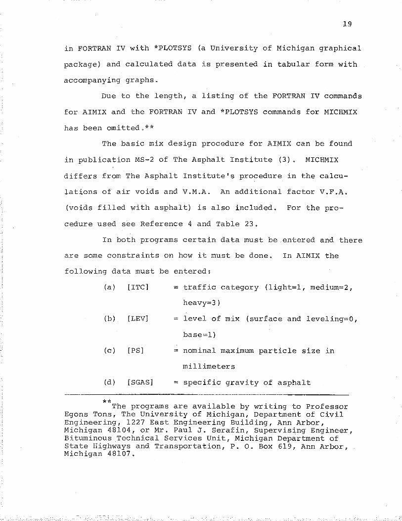
In both programs certain data must be.entered and there
are some constraints on how it must be done. In AIMIX the
following data must be entered:
(a) [ITC] = traffic category (light=l, medium=2,
heavy=3)
(b) [LEV] = level of mix (surface and leveling=O,
base=l)
(c) [PS] = nominal maximum particle size in
millimeters
(d) [SGAS] = specific gravity of asphalt
** The programs are available by writing to Professor Egons Tons, The University of Michigan, Department of Civil Engineering, 1227 East Engineering Building, Ann Arbor, Michigan 48104, or Mr. Paul J. Serafin, Supervising Engineer, Bituminous Technical Services Unit, Michigan Department of State Highways and Transportation, P. 0. Box 619, Ann Arbor, Michigan 48107.
20
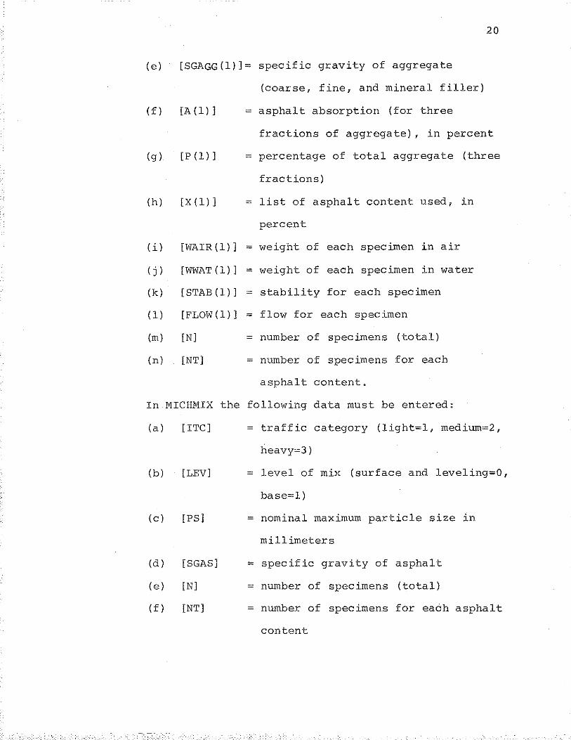
(e) [SGAGG(l)]= specific gravity of aggregate
(coarse, fine, and mineral filler)
(f) [A ( l) ]
(g) [P(l)]
(h) [X(l)]
(i) [WAIR(l)]
( j ) [WWAT (l)]
(k) [STAB ( l)]
( l) [FLOW(l)]
(m) [N]
(n) [NT]
In MICHMIX the
(a) [ITC]
(b)
(c)
(d)
(e)
(f)
[LEV]
[PS]
[SGAS]
[N]
[NT]
= asphalt absorption (for three
fractions of aggregate), in percent
= percentage of total aggregate (three
fractions)
= list of asphalt content used, in
percent
= weight of each specimen in air
= weight of each specimen in water
= stability for each specimen
= flow for each specimen
= number of specimens (total)
= number of specimens for each
asphalt content.
following data must be entered:
= traffic category (light=l, medium=2,
heavy=3)
= level of mix (surface and leveling=O,
base=l)
= nominal maximum par-ticle size in
millimeters
= specific gravity of asphalt
= number of specimens (total)
= number of specimens for each asphalt
content
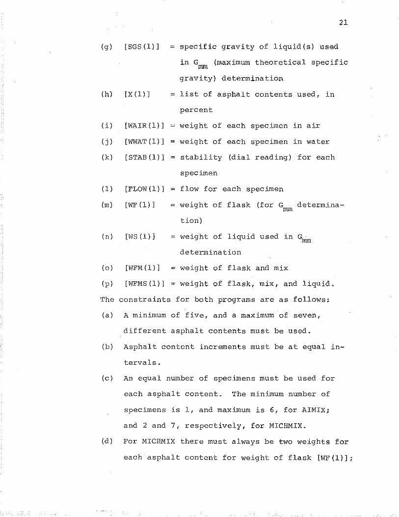
21
(g) [SGS (1)] = specific gravity of liquid (s) used
in Gmm (maximum theoretical specific
gravity) determination
(h) [X(l)] = list of asphalt contents used, in
percent
(i) [WAIR(l)] =weight of each specimen in air
(j) [WWAT(l)] =weight of each specimen in water
(k) [STAB(l)] = stability (dial reading) for each
(1)
(m)
( n)
specimen
[FLOW(l)] =flow for each specimen
[WF(l)] =weight of flask (for G determinamm
[WS (1)]
tion)
= weight of liquid used in Gmm
determination
(o) [WFM(l)] = weight of flask and mix
(p) [WFMS(l)] =weight of flask, mix, and liquid.
The constraints for both programs are as follows:
(a) A minimum of five, and a maximum of seven,
different asphalt contents must be used.
(b) Asphalt content increments must be at equal in-
tervals.
(c) An equal number of specimens must be used for
each asphalt content. The minimum number of
specimens is 1, and maximum is 6, for AIMIX;
and 2 and 7, respec·tively, for MICHMIX.
(d) For MICHMIX there must always be two weights for
each asphalt content for weight of flask IWF(l)];
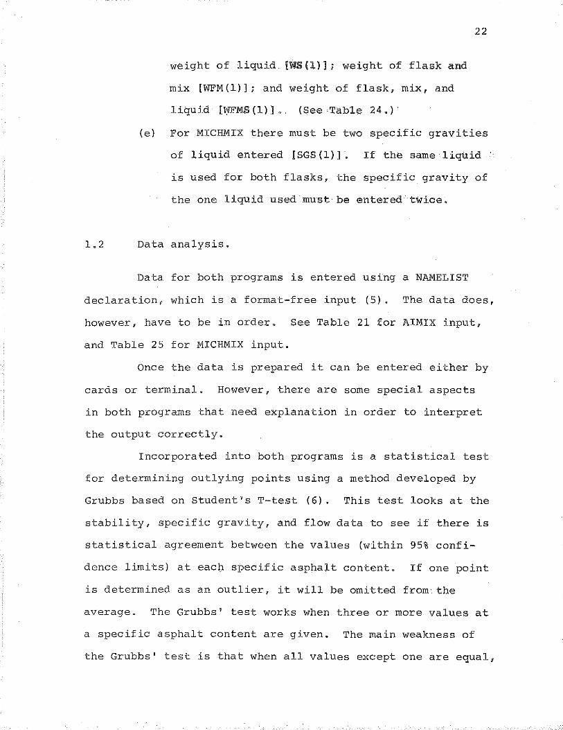
weight of liquid [WS{l)]; weight of flask and
mix [WFM(l)]; and weight of flask, mix, and
liquid ll:i'FMS (1)].. (See Table 24.) ·
22
(e) For MICHMIX there must be two specific gravities
of liquid entered [SGS (1)] • If the same liquid ·
is used for both flasks, the specific gravity of
the one liquid used must be entered twice.
1.2 Data analysis.
Data for both programs is entered using a NAMELIST
declaration, which is a format-free input (5). The data does,
however, have to be in order. See Table 21 for AIMIX input,
and Table 25 for MICHMIX input.
Once the data is prepared it can be entered either by
cards or terminal. However, there are some special aspects
in both programs that need explanation in order to interpret
the output correctly.
Incorporated into both programs is a statistical test
for determining outlying points using a method developed by
Grubbs based on Student's T-test (6). This test looks at the
stability, specific gravity, and flow data to see if there is
statistical agreement between the values (within 95% confi
dence limits) at eaCD specific asphalt content. If one point
is determined as an outlier, it will be omitted from the
average. The Grubbs' test works when three or more values at
a specific asphalt content are given. The main weakness of
the Grubbs' test is that when all values except one are equal,
23
the one not equal will be eliminated as an outlier. Take the
flow values of 9, 9, 9 and 11. The 11 value will be deter
mined as an outlier and will be omitted--which may be un
desirable. However, in both programs the Grubbs' test has
been modified for the flow test values. The reason for this
modification is that the flow readings are rounded-off values
(to the nearest interger) and this affects the distribution
unfairly. If a flow value has been determined outlier, the
other values are checked to see if they are equal to each
other. If not, the extreme point is omitted; if they are
equal, then the extreme point is checked to see if it is
within 20% of the average. If it is within 20% of the
average, it is kept. Otherwise, it is omitted.
Also, in both programs, stability dial readings can
be read in directly if the calibration constant is written
into the program. In MICHMIX this has already been done to
accommodate the present MDSHT equipment. In AIMIX it has not.
The instruction
XSTAB(I,J) = CF* YSTAB(!,J).
can be changed to
XSTAB(I,J) = CF* YSTAB(I,J)* 15.
where 15 is the calibrative constant, for example, to accommo
date directly entering of dial readings. The program also
adjusts the stability according to the volume of the specimen.
The correc·tion factor for adjusting the stability was derived
by running a regression analysis of the values presented
in MS-2 Table III-1 (3). The factor was found to be expressed
24
best by the third degree polynomial,
where
CF = -l.027xl0-? (VOL) 3 + 1.657xl0-4 (VOL) 2
-.09143(VOL) + 18.19,
CF =correction factor,
VOL = volume of specimen in cubic centimeters.
This correction factor will introduce some variance
from the tabular values in MS-2 Table III-1, but not over 3%.
When analysis of Marshall data is done conventionally,
graphs are drawn using the calculated and observed data. Both
AIMIX and MICHMIX use the least-square method of regression to
fit curves to the data. In AIMIX, second and third degree
polynomials are fitted to the five plots: specific gravity,
stability, air voids, V.M.A., and flow vs. asphalt content by
weight of mix. The correlation coefficient of the second and
third degree polynomials are compared, and the equation with
the highest coefficient is selected. In MICHMIX all regres
sions, except for flow vs. asphalt contents, are the compari
sons between second and third degree polynomials. Maximum
theoretical specific gravity vs. asphalt content is theoret
ically a straight line, and a first degree polynomial is fitted.
The curve fitting routine is also equipped with 95% upper and
lower confidence limits to determine if any of the average
points lie outside this range. If they do, then the point is
omitted and another regression is run.
Both programs also give the optimum asphalt content
which is the average of:
(a) Asphalt content at maximum stability.
(b) Asphalt content at max~mum spec~f~c gravity.
(c) Asphalt content providing proper air voids
(4% air voids for surface and leveling, 5.5%
for base) .
25
If it is impossible to design the mix for the proper
air voids, a message on the output will be printed:
***CANNOT DESIGN FOR PROPER AIR VOIDS WITHIN GIVEN ASPHALT
CONTENT RANGE***
The optimal asphalt content given in this case will
be the average of the asphalt content at maximum stability
and the asphalt content at maximum specific gravity.
Error messages will also be printed for a deficiency
in V.M.A. or a flow outside the acceptable range (reference
to MS-2 (3) ) .
An output example for AIMIX is shown in Table 22.
The input data is taken from the example in MS-2 as shown in
Table 20. Figure 42 shows graphs drawn using the regression
values from AIMIX.
It can be seen from the examples presented that the
program does a generally good job of analysis. The co.mpari
son between AIMIX and the example from MS-2 (Table 20) is
good.
AIMIX MS-2
Asphalt content at maximum stability 4.56 4.8
Asphalt content at maximum specific gravity 5.15 5.1
Asphalt content providing proper air voids 4.36 4.3
Optimum asphalt content 4.69 4.7
An output for MICHMIX is shown in Table 26. The
graphical output shown in Figures 43 to 49 can be obtained
on a plotter or a cathode ray tube terminal.
26
The asphalt content of 4.88% at maximum stability for
this example may be low (Table 26, page 3). Otherwise,
MICHMIX's curve fitting routines seemed to do well.
The Grubbs' test did throw out some values in both
design examples which probably should not have been. This
was due ·to all but one point being nearly equal. However, if
the values are all approximately equal and one is omitted,
the average will change little (example from Table 26,
page 3- 1488*, 1465, 1461, 1466).
1.3 Advantages of the program.
The advantages of AIMIX and MICHMIX are several, First
there is a savings in time. It takes approximately one-half hour
to prepare, input, receive, and interpret the data for each mix
design. Conventional data analysis takes much longer. It takes
MDSHT approximately 8 man-hours for each mix design to analyze
Marshall data by conventional methods. The second advantage
is that there are no computational errors. Third, least-
square regression provides an excellent curve fit if the data

27
is reasonable. Fourth, with no computational errors and a
better curve fit, generally a better optimum asphalt content
value can be obtained. Fifth, a very neat and professional
looking report is achieved. The MDSHT has already adopted
MICHMIX for operational use.
1.4 Special precautions
If one is to use either MICHMIX or AIMIX, two recom
mendations are pertinent:
(a) Use at least 4 specimens for each asphalt content
(this helps to establish more real·istic limits
for the Grubbs' test and should give truer
averages at each asphalt content) .
(b) Graphs should always accompany each design and
they should be analyzed. The output from the
two programs is always subject to human review.
2. Further Work on Mix Design Factors
2.1 Previous work.
Many attempts have been made to define the geo
metric characteristics of aggregates to facilitate a unified
bituminous mixture design procedure. The packing volume con
cept of Tons and Goetz (7) served as the basis of previous
work. Tons and Ishai (8) refined this concept to develop a
simple pouring test which would evaluate the particle charac
teristics of shape, angularity or roundness, and roughness or
surface texture. Using the common aggregate parameters of
apparent specific gravity, bulk specific gravity, and water
absorption along with the derived pouring test parameters,
an accurate prediction of overall particle irregularity can
be made. Tons et al. (7) defined the packing volume of a
particle as the volume enclosed under a thin membrane
28
stretched along the particle surface, as shown in Figure 50.
The term rugosity has been used to describe the ratio of the
volume of asphalt lost under this imaginary membrane to the
surface area of the membrane.
Using the rugosity values obtained for specific
fractions of the overall aggregate mixture and considering
interaction of particles of various sizes, a mixture design
program was developed. A revised version of this program is
shown in Appendix B. Aggregate factors vital to this program
may also be calculated by computer, and this aggregate
parameter program is shown in Appendix A.
2.2 Calibration of pouring test apparatus for rugosity determination.
Considerable time was spent on standardization and
calibration of apparatus used in the pouring test. A variety
of pouring tests were performed using aggregates, glass beads,
and precision steel ball bearings of various sizes with
different types and sizes of orifices and different sizes of
catch containers. Table 27 shows a compilation of the various
container sizes and bead types and sizes used in the tests.
29
Glass beads and steel ball bearings were also hand-packed into
various containers in the hope of establishing a practical
limit of packing for each sphere-container combination.
Appendix C illustrates the pouring test apparatus and in
dicates the two previously used fraction-container size combi
nations. A new container size spectrum is also proposed
based on present knowledge of pouring test parameters.
Significance of the following factors was evaluated:
(a) Pouring time.
(b) Pouring height.
(c) Orifice size.
(d) Orifice type.
(e) Container-particle volume ratio for standard
beads.
(f) Container-particle volume ratio for aggregates.
(g) Variability of standard beads.
(h) Catch container volume-area ratio.
(i) Ratio of volume poured to volume caught.
(j) Catch container shape.
It may be assumed that as particles are poured more
slowly, mutual interference between them will decrease,
resulting in higher packing density. This assumption was
verified by Tons and Ishai (8) and present tests agreed with
previous findings.
Pouring height was also found to be significant.
Tests performed with P#8-R#l0 crushed gravel using a one
inch cone orifice and 234 ml. catch container gave an
30
approximately linear relationship between pouring height and
caught weight of aggregate as shown in Figure 51. A similar
series of tests were performed with l, 3, 4, 5 and 6 mm. glass
beads and here the caught weight increase was not quite linear
at heights greater than 3-4 inches. The relationship example
for 3 mm. beads is shown in Figure 52.
The previously used pouring height of 21 em. (approx.
8 in.), while in the non-linear range for the glass beads,
has worked well. Previous research with fourteen experimental
aggregates used this pouring height as a standard, and mix
designs based on the rugosity values obtained were in close
agreement with Marshall mix designs. For future designs, how
ever, small adjustments are proposed from this study.
The factor of pouring orifice size is significant in
that it directly affects pouring time. Orifice size must be
chosen to allow particles to pour slowly, but must be kept
large enough to preclude bridging of particles. Although
particle bridging and the resultant intermittent pouring did
not significantly affect caught weight, such slow pouring is
time consuming and not necessary to insure packing optimiza
tion.
Orifice type also had a pouring time related effect.
For purposes of tests, orifices were defined as being either
plate type or cone type as illustrated by Figure 53. Opening
type is significant only for large opening/particle size
ratios (8-10) . This is due to the fact that the cone type
orifice significantly reduces pouring time, as the rock
31
particles can slide down the smooth cone sides more easily.
The opening type was insignificant at small opening/particle
size ratios. This behavior is predicted by the caught weight-
pouring time relationship mentioned previously, which in-
dicated no further significant increase in caught weight
beyond a sufficiently long pouring time. Beyond such a point
it is immaterial whether pouring time is increased by a re-
duction in opening size or a change of opening type.
The ratio of catch container volume to the volume of
an individual particle was found to have a very significant
effect on packing of standard beads. Extensive work was
done to define this effect. Figure 54 shows the relationship
for a wide range of standard beads (smooth, spherical par-
ticles) and containers where hand packing of beads was
employed. When such behavior was observed in hand packing
tests, it was logical to predict a similar phenomenon in
pouring tests. A test was designed to define the relation-
ship statistically. Appendix D describes the conduct of
this test and presents a method to adjust packing specific
gravity to counteract volume ratio effects.
Unlike the smooth particles, aggregates packed uni-
formly well for most ratios of container volume to individual
particle volume. Figure 55 shows the results of a series
of tests performed with Pl"-R3/4" and P3/4"-Rl/2" slag frac-
tions. In these tests, although the container volume-particle
volume ratio varied widely, the statistical analysis of
variance shows no significant difference in packing efficiency
MICHIGAN DEPARTMENT OF
TRANSPORTATION LIBRARY LANSING 48909
for the range considered for the two aggregate sizes. In
light of these tests, we may conclude that the rough aggre
gate particles are not much affected by container boundary
effects.
32
Consider the simultaneous analysis of the rough
aggregate and the smooth spheres used as a basis for pack
ing specific gravity. As explained in detail in Appendix D,
the boundary effects for the beads may be corrected statis
tically. The rough aggregate particles need no correction
for boundary effects. Now, both the smooth beads and the
rough aggregate particles may be viewed as randomly packed
particles occupying some small portion of an infinitely
large collection of particles. As such, the difference in
volumes occupied by the respective smooth and rough particles
in this small portion of the mass will differ by only the
rugosity volume.
Two other parameters associated with the test apparatus
were found to be insignif1cant. The ratio of catch container
volume to catch container inside surface area was found to be
insignificant, as demonstrated in Appendix D. The ratio of
volume poured to volume caught was also found to be insignifi
cant for ratios between 1.1 and 1.7. Table 29 shows the
results of the statistical analysis.
Present research was directed at standardizing catch
container shape rather than evaluating container shape as
such. All catch containers were constructed by modifying
commercially available stainless steel griffin beakers. To
alleviate as many variables as possible, it is recommended
that all catch containers be right circular cylinders, the
bottom-side intersection having a circular radius at l~ast
as large as that of the standard beads to be poured into
it. The dimensions of the 250 ml. and 600 ml. containers
are shown in Figure 56.
33
Having determined the relative significance of each
pouring test variable, the following recommendations may be
made for calibrating pouring test apparatus:
(a) For a given size aggregate fraction, select a
catch container from Table C-1, Appendix C.
(b) Determine catch container volume by any con
venient and reliable method, i.e., mensuration
formula, water calibration, etc.
(c) Standard smooth particles (glass beads) should
be used to represent particles with zero rugosity
for comparison purposes in the pouring test. A
bead size is specified in Table C-1, Appendix c,
for any fraction size, and in general standard
bead diameter should be approximately the same
as the diameter of the aggregate particle it is
intended to represent. Properties of the standard
beads which must be determined are apparent spe
cific gravity and coefficient of deviation of
bead weight. The latter can be determined with
sufficient accuracy by weighing 20 to 50 beads
individually. For beads smaller than 1 mm.
34
diameter, this is not practical, and no correc-
tion for bead size variability is considered
in this range.
(d) Select an orifice diameter which will allow
aggregate or beads to flow as slowly as possible
without bridging within the cone. The same size
orifice need not be used for both the aggregate
fraction and the associated standard bead, but
an orifice size should be chosen based on flow
characteristics of the material being poured.
As a guide, the first trial orifice size should
be chosen with diameter approximately 6-8 times
the diameter of the particle being poured.
2.3 Comparison of calculated asphal·t content with Marshall optimum asphalt content.
Based on the aggregate factors determined for each
fraction of an aggregate blend, a prediction of optimum
asphalt content may be made as recommended in Appendix E.
The work of Tons and Ishai (8) dealt with a six-fraction mix.
In an effort to illustrate the applicability of the packing
factor concept on a broader scale, it was decided to compare
the calculated optimum asphalt content for seven gravel mixes
recently used by the Michigan Department of State Highways
and Transportation. The optimum asphalt content for these
mixes was determined by the Marshall mix design method. A
typical MDSHT design data sheet is shown in Tables 30 and 31.
35
Table 32 shows the composition of the various aggregate
blends by size of aggregate. Since the actual aggregates used
in the mix design specimens were not available, packing spe-
cific gravity values were based on a weighted mean of natural
and crushed gravel parameters determined by Tons and Ishai
for Michigan sources (8). Because maximum specific gravity
and asphalt content tests were not run on each fraction, it
was considered the same for all fractions. Water absorption
was taken as the weighted mean of the absorptions of the ag-
gregates making up the individual fractions. Flyash, used
as a mineral filler, was considered to have an absorption of
zero. Although this is not completely correct, the amount
used in each mix was very small, and the simplification was
not considered to be a serious departure.
As detailed in Appendix E, selection of an optimum
asphalt content was based on a minimum calculated packing
V.M.A. in conjunction with an air void content of 4"' 0 • It
must be noted that compaction of a number of Marshall speci-
mens is necessary for optimum asphalt prediction, since
for any particular asphalt content, we must know mix specific
gravity at that content as a result of a standardized com-
paction effort. Knowing the mix specific gravity for any
asphalt content, we can easily enter the design tables and
determine packing V.M.A. As in the Marshall method of mix
design, it is best to bracket the optimum value with trial
specimens. As shown in Table 33 optimum asphalt contents
predicted by this method agree closely with MDSHT design
36
values.
From the work done so far, it is apparent that for the
time being the Marshall approach is a useful practical method
for designing mixes. The future outlook for a more "funda
mental" mix design is good, but more work is needed to elimi
nate the necessity for a trial-and-error specimen making and
testing.
CONCLUSIONS
The conclusions are concerned with the two parts of
this report, namely: (a) grading of asphalts by viscosity
at 25 C, and (b) computerized bituminous concrete design.
On the basis of work done so far, the following is pertinent:
(a) A workable method for measuring asphalt viscosity
at 25 c has been developed using the cone-plate
viscometer. -2 -1 At the shear rate of 2xl0 sec ,
18 samples per 8-hour day can be tested.
(b) USING THE VISCOSITY AT 25 C AS A STANDARD, PRAC-
TICAL VISCOSITY CHARTS FOR ASPHALT CEMENTS FOR
SIX SOURCES (SUPPLIERS) IN MICHIGAN HAVE BEEN
DEVELOPED. A DESIRED VISCOSITY (HARDNESS)
ASPHALT (AT 25 C) CAN BE SPECIFIED ON THE BASIS
OF VISCOSITY AT 135 C AND 60 C SO THAT THE
SUPPLIER DOES NOT HAVE TO MEASURE VISCOSITY AT
25 c.
(c) Specification limits for viscosity due to aging
of different asphalt cements have also been·pro-
duced in a graphical form.
(d) The constant rate penetration test at 25 C showed
a better correlation with viscosity (at 25 C)
than the regular and submerged penetration tests.
More work in this area is needed.
37

(e) A PRACTICAL COMPUTERIZED PROCEDURE HAS BEEN
PRESENTED FOR CALCULATIONS IN THE DESIGN OF
BITUMINOUS CONCRETE MIXES USING A MODIFIED
MARSHALL TEST PROCEDURE AS THE BASIS.
(f) The mix design method gives both numerical and
graphical display of the results to be used
for engineering decisions.
38
(g) Additional work on mix design using fundamental
properties of materials has indicated promise
for further design improvements in the future.
RECOMMENDATIONS
(a) The viscosity grading approach should be tried
as soon as possible to make minor adjustments
where necessary.
(b) The cone-plate viscometer with 18 tests per day
is still not a very fast method to determine
asphalt viscosity at 25 C. Further work on
simplified viscosity measuring methods is
desirable, if time and funds permit.
(c) The Marshall method is a good practical way for
designing mixes, even though it involves certain
amount of trial-and-error testing .. Future
pursuits towards a more "fundamental" design
method should be of interest.
39

BIBLIOGRAPHY
BIBLIOGRAPHY
1. Egons Tons, Tsuneyoshi Funazaki and Richard Moore, "Low Temperature Measurement of Asphalts for Viscosity and Ductility," Research Report, The University of Michigan, Department of Civil Engineering, December, 1974.
2. Egons Tons and Alfred P. Chritz, "Grading of Asphalt Cements by Viscosity," Technical paper presented at ·the Annual Meeting of The Association of Asphalt Paving Technologists, February, 1975.
3. The Asphalt Institute, "Mix Design Methods for Asphalt Concrete," MS-2, October, 1969.
4. P. J. Serafin, "Measurement of Maximum Theoretical Specific Gravity of a Bituminous Mixture," Michigan Department of State Highways, June, 1956.
5. B. Carnahan and J. 0. Wilkes, "Digital Computing, Fortran IV, WATFIU, and MTS," The University of Michigan, Chemical Engineering Department, 1973.
6. F. E. Grubbs, "Sample Criteria for Testing Outlying Observations," Ann. Math. Stat., 21:27-58 (1950).
7. Egons Tons and w. H. Goetz, "Packing Volume Concept for Aggregates," Research Report No. 24, Joint Highway Research Project, Purdue University, September, 1967.
8. Egons Tons and Ilan Ishai, "Design Factors for Bituminous Concrete," Research Report, The University of Michigan, Department of Civil Engineering, May, 1973.
9. D. J. Fox and K. E. Guire, "Documentation for Michigan Interactive Data Analysis System," 2nd Ed., The Statistical Research Laboratory of The University of Michigan, September, 1973.
41

TABLES
SAMPLE- 75B-30(120-150)#5
TEMP - 25 C
LARGE CONE - THIN STRING
Weight (g)
500
200
500
Degrees
1
1
1
TABLE 1
TYPICAL VISCOSITY RUN DATA
Time (sec)
57.7
145.7
57.9
t/8 (sec/deg)
57.7
145.7
57.9
Viscosity (poises)
4.42x10 5
5 4.47x10⁵~4.46x10⁵ 4.44x10 Y
Shear Rate (sec:-1)
-2 1.39x10 -2 3.50x10
.... w
Sample Identification No. MDSHT Pen.
Code No. Grade
l 73B-1
2 73B-2
3 73B-3
4 73B-4
5 73B-5
6 73B-6
7 73B-7
8 73B-ll
9 73B-l2
10 73B-13
ll 73B-17
12 738-18
13 73B-l9
14 73B-21
15 73B-22
16 738-23
l7 74B-1
18 74B-2
19 74B-3
20 748-4
21 74B-5
22 74B-6
60-70
85-100
120-150
200-250
60-70
85-100
120-150
120-150
200-250
85-100
200-250
85-100
120-150
60-70
85-100
120-150
60-70
85-100
120-150
200-250
60-70
85-100
TABLE 2
AVERAGE PENETRATION AND VISCOSITIES - ORIGINAL ASPHALTS
Sample Source
I - '72
I - '7 2
I - I 72
I - I 72
A- '72
A- '72
A - '72
c- '72
c - '72
D - '72
E - I 7 2
G - I 72
G - I 72
N- '72
N- '72
N- '72
G - I 74
G - I 74
G- '74
G - '74
N - '74
N- '74
Standard Penetration @
25 c
63
86
128
245
59
91
137
133
236
79
220
87
134
63
83
14 5
71
101
133
210
64
99
@
25 c
2.44xlo 6
9.32x10 5
4.65x10 5
1.44x1o5
6 2.45x10
9.16x10 5
4.56x1o5
4.84x1o5
5 1.56x10
6 1. 23x10
l.88x1o 5
l. 04x1o 6
4.72x1o 5
3.25x1o 6
1.12x1o 6
3.57x1o 5
l. 91x1o 6
8.72x1o5
4.88x1o 5
l. 95x1o 5
1.94x1o6
8.12x10⁵
Viscosity (Poises) @ @ @
60 c 107 c 121 c
2840
1270
790
387
2140
1200
629
870
430
1690
372
1590
885
2340
1460
784
2660
1510
943
569
2460
1300
23.35
14.70
' 19.10
7.08
17.58
13.06
8. 98
10.95
7.82
15.58
6.78
15.68
12.00
20.60
13.46
10.63
18.93
14.99
10.67
8. 36
18.47
14.02
9.62
6.26
4.65
3.33
6.64
5.21
3.65
4.97
3.52
6.06
3.12
6.41
4.68
7.74
5.63
4.43
8.24
6.18
5.30
3.87
7.79
5.07
@
135 c
5.24
3.46
2.74
1. 99
3.63
2.86
2.11
2.90
2.20
3.42
l. 93
3.42
2.70
3.92
3.19
2.41
4.56
3.50
3. 03
2.15
4.13
2.97
Sample Identification No. MOSHT Pen.
Code No. Grade
23 74B-7
24 74B-8
25 74B-9
26 74B-10
27 74B-ll
28 74B-12
29 74B-l3
30 74B-l4
31 748-15
32 748-18
33 74B-19
34 74B-2l
35 74B-22
36 748-23
37 74B-24
38 74B-25
39 74B-26
40 74B-27
41 74B-28
42 74B-29
43 74B-30
44 73B-9
45 738-16
120-150
200-250
85-100
120-150
200-250
60-70
85-100
120-150
200-250
120-150
200-250
85-100
60-70
85-100
120-150
200-250
60-70
8 5-100
120-150
200-250
85-100
60-70
120-150
Sample Source
N - '74
N - I 74
J - '74
J - I 74
J - '74
I - I 74
I - I 74
I - I 74
I - I 74
p - '74
P - I 74
Q - '74
A - '74
A - '74
A - '74
A - '74
E - '74
E - '74
E - 1 74
E - I 74
Q - I 74.
c - . 7 2
E - '7 2
TABLE 2 (Continued) Page 2
Standard Penetration @
25 c
132
2 37
90
128
249
63
89
134
244
159
289
96
69
95
124
235
68
82
125
226
87
64
119
@
25 c
4.63x1o 5
1. 74x10 5
1. 07x1o 6
4.88x10 5
l. 61x105
2.60x10⁶
9.83x1o5
4.74xlo 5
1. 63x1o 5
5.50x1o5
5 2.08x10
8.04x10 5
2.33x1o6
l. 03x106
5.60x1o 5
1.69x10⁵
2.42x10⁶
l. 33x106
5.54x10 5
5 1. 94x1 0
1. 30x1o6
Viscosity (Poises) @ @ @
60 c 107 c 121 c
771
402
1710
1010
480
3130
1230
861
392
387
161
817
1840
1110
721
354
1930
1230
683
388
1410
2680
720
9.31
6.59
14.38
10.85
6.88
21.62
13.85
10.59
6.63
5.40
3.22
9.23
16. 55
9. 85
7. 71
5. 08
14.28
11.15
8.10
6.02
12.75
21.38
9.54
. 4. 25
3.06
6.33
4.39
3.20
9.33
6.19
5.00
3.26
2.57
1. 62
4.05
5.46
4.48
3.54
2.43
6.41
5.20
3.88
2.88
5.58
9.41
4.50
@
135 c
2.51
1. 83
3. 71
2.86
1. 98
5.36
3. 68
3.07
2.03
1. 59
1. 04
2.35
3.42
2.72
2.25
1.50
3.71
3.11
2.36
1. 81
3.36
4.54
2.72
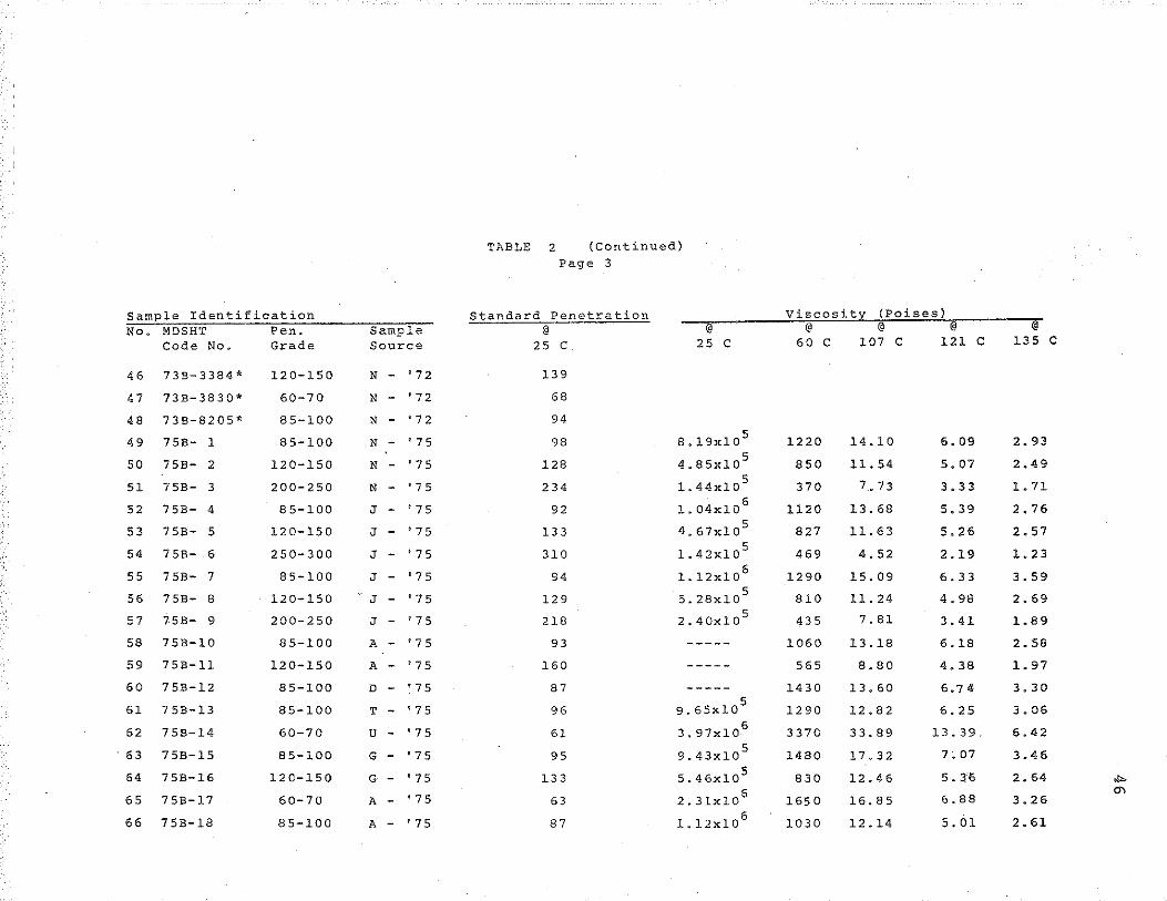
TABLE 2 (Continued) Page 3
Sample Identification Standard Penetration Viscosity (Poises) No. MDSHT Pen. Sample @ @ @ @ @ @
Code No. Grade Source 25 c. 25 c 60 c 107 c 121 c 135 c
46 738-3384* 120-150 N - '72 139
47 73B-3830* 60-70 N - '72 68
48 738-8205* 85-100 N - '72 94
'75 5
1220 14.10 6.09 2.93 49 758- 1 85-100 N - 98 8.19xl0
50 75B- 2 120-150 N - '75 128 4.85xl0 5
850 11.54 5.07 2.49
51 75B- 3 200-250 N - '75 234 1.44x10 5
370 7. 73 3.33 l. 71
52 75B- 4 85-100 J - '75 92 . 6
l. 04x10 ll20 13.68 5.39 2.76
53 75B- 5 120-150 J - '75 133 4.67x1o5
827 11.63 5.26 2.57
54 758- .6 250-300 '75 310 5
469 4.52 2.19 1. 23 J - 1.42x10
55 758- 7 85-100 J - '75 94 l.l2x106
1290 15.09 6.33 3.59
56 758- 8 120-150 J - '75 129 5.28x10⁵
810 11.24 4. 98 2.69
57 758- 9 200-250 J - '75 218 2.40x10⁵
435 7.81 3.41 1.89
58 758-10 8 5-100 A - '75 93 1060 13.18 6.18 2. 58
59 75B-ll 120-150 A - '75 160 565 8.80 4.38 l. 97
60 758-12 85-100 D - '75 87 1430 13.60 6. 7 4 3.30
61 758-13 85-100 T - '75 96 9.65x10 5
1290 12.82 6.25 3.06
62 758-14 60-70 '75 6 3370 33.89 13.39. 6.42 u - 61 3.97x10
63 7 5B-l5 85-100 '75 95 5 1480 17.32 7; 07 3. 46 G - 9.43x10
64 758-16 120-150 G - '75 133 5.46x1o 5 830 12.46 5. 3'6 2. 64 ,. 2.31x10
6 "' 65 75B-17 60-70 A - '75 63 165 0 16.85 6.88 3.26
66 75B-18 85-100 A - '75 87 l.12x10 6
1030 12.14 5.01 2.61
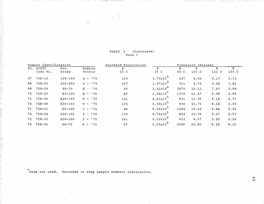
TABLE 2 {Continued) Page 4
Sam:ele Identification Standard Penetration Viscosity {Poises} No. MDSHT Pen. Sample @ @ @ @ @ @
Code No. Grade Source 25 c 25 c 60 c 107 c 121 c 135 c
67 758-19 120-150 '75 5
8.65 4.17 2.13 A - 129 5.75x10 627
68 758-20 200-250 A - '75 237 1.97x10⁵
311 6.74 3.06 1. 61
69 75B-24 60-70 E - '75 63 2.41x10 6 2870 18.12 7.87 3.46
70 7 58-25 85-100 E - '75 88 1. 36x106
1370 14.97 6.38 3.09
71 75B-26 120-150 '75 5
831 12.08 5.12 2.71 E - 122 6.41x10
72 758-30 120-150 u - '75 135 4.50x10⁵ 920 13.74 6.16 3.05
73 758~31 ·85-100 I - '75 98 8.62x1o 5 1260 15.49 6.66 3.26
74 758-32 120-150 '75 139 5
653 10.78 5. 07 2.53 I - 4.74xl0
75 . 758-33 200-250 '75 241 5 423 8.57 3.95 2.10 I - 2.02xl0
76 758-34 60-70 '75 6
2090 22.86 8.28 4.15 D - 69 2.05x10
• Data not used~ Included to keep sample numbers consecutive.
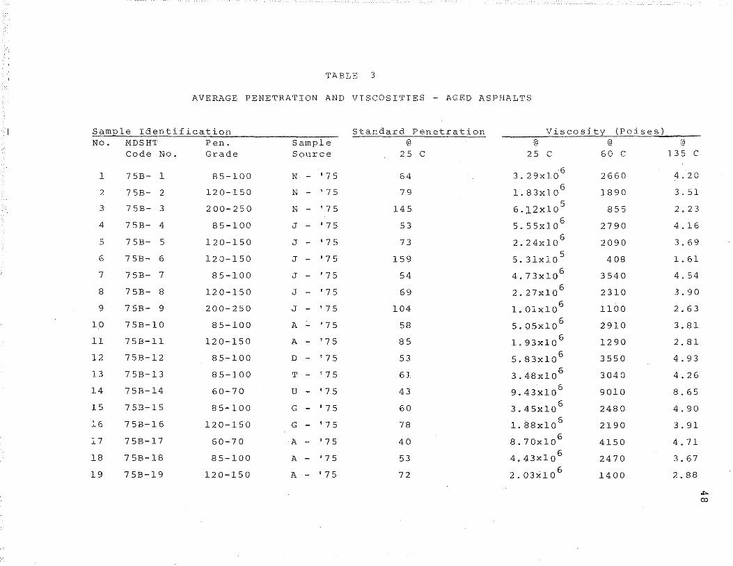
TABLE 3
AVERAGE PENETRATION AND VISCOSITIES - AGED ASPHALTS
SamJ2le Identification Standard Penetration Viscosity (Poises) No. MDSHT Pen~ Sample @ @ @ @
Code No. Grade Source 25 c 25 c 60 c 135 c
1 75B- 1 85-100 N - '75 64 ·6
3.29xl0 2660 4.20 6
1890 3. 51 2 75B- 2 120-150 N - '75 79 1.83xl0 5 2.23 3 7 5B- 3 200-250 N - '75 145 6.12xl0 855 6 4.16 4 75B- 4 85-100 J - '75 53 5. 55xl0 2790
120-150 73 6 2090 3.69 5 75B- 5 J - '75 2.24xl0
6 120-150 '7 5 159 5 4 08 1. 61 75B- 6 J - 5.3lxlo
7 75B- 7 85-100 '75 54 6 3540 4.54 J - 4.73xlO
8 75B- 8 120-150 '75 69 6 2310 3.90 J - 2.27x10
9 7 SB- 9 200-250 '75 104 6 1100 2.63 J - 1. Olxl 0
10 75B-10 85-100 '75 58 6 2910 3.81 A - 5.05xl0
11 75B-11 120-150 A '7 5 85 6 1290 2.81 - 1.93xlO
12 75B-12 85-100 D '7 5 53 6 3550 4.93 - 5.83xl0
13 75B-13 85-100 T '75 61 6 3040 4.26 - 3.48xl0
14 75B-14 60-70 u '75 43 6 9010 8.65 - 9.43xl0
15 75B-15 8 5-10 0 G '75 60 6 2480 4.90 - 3.45xlO
16 75B-16 120-150 '75 78 6 2190 3.91 G - 1. BBxlO
758-17 6 4.71 17 60-70 A - '75 40 B.70x1o 4150
18 758-18 85-100 A - '75 53 4.43x1o 6 2470 3.67
19 758-19 120-150 '75 72 6 1400 2.88 A - 2.03x10
,. a:>
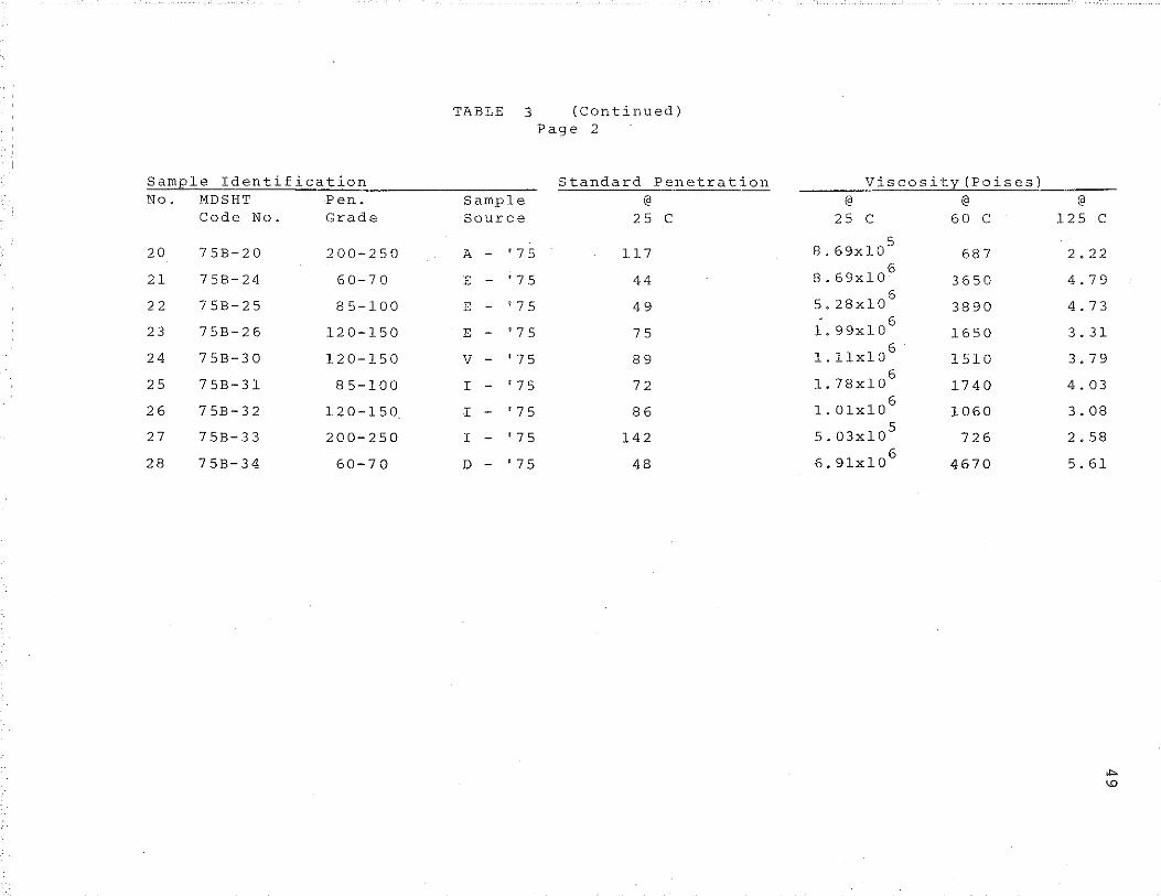
TABLE 3 (Continued) Page 2
Sample Identification Standard Penetration Viscosity(Poises) No. MDSHT Pen a Sample @ @ @ @
Code No. Grade Source 25 c 25 c 60 c 125 c 5
20 7 5B- 2 0 200-250 A - '75 117 8.69xl0 687 2. 2 2 6
21 75B-24 60-70 E - '75 44 8.69xl0 3650 4.79 6
22 75B-25 85-100 E - • 7 5 49 5.28xl0 3890 4.73 . 6
23 75B-26 120-150 E - '75 75 l.99xl0 1650 3. 31 6
24 75B-30 120-150 v - '75 89 l.llxlO 1510 3. 7 9 6
25 75B-31 85-100 I - '75 72 l.78xl0 1740 4. 03 6
26 7 5B-3 2 120-150 .I - '75 86 l. OlxlO 1060 3.08
27 75B-33 200-250 I - • 7 5 5
142 5.03xl0 726 2.58
28 75B-34 60-70 D - '75 6
48 6.9lxl0 4670 5.61
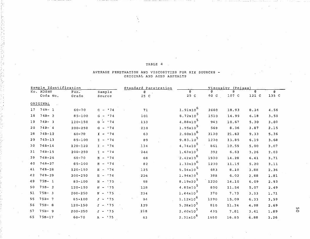
TABLE 4
AVERAGE PENETRATION AND VISCOSITIES FOR SIX SOURCES -ORIGINAL AND AGED ASPHALTS
Sarn;ele Identification Standard Penetration Viscosity {Poisesl No. MDSHT Pen. Sample @ @ @ @ @ @
Code No. Grade Source 25 c 25 c 60 c 107 c 121 c 135 c
ORIGINAL
17 74B- 1 60-70 G - '74 71 1.9lx106 2660 18.93 8.24 4.56
18 74B- 2 8 5-l 00 G - '74 101 8.72x1o 5 1510 14.99 6.18 3.50
19 74B- 3 120-150 G - '74 133 4.88x1o5
943 10.67 5.30 3. 03
20 74B- 4 200-250 G - '74 210 1.95xl05 569 8.36 3.87 2.15
28 748-12 60-70 I - '74 63 2.60x10⁶
3130 21.62 9.33 5.36
29 74B-13 85-100 I - 1 74 89 9.83.10 5 1230 13.85 6.19 3. 68
30 74B-14 120-120 I - '74 134 4.74x1o5
861 10.59 5.00 3.07
31 748-15 200-250 I - '74 244 1.63xlo5
392 6.63 3.26 2. 03
39 74B-26 60-70 E - '74 68 2.42xlo 6 1930 14.28 6.41 3.71
40 748-27 8 5-100 E - 1 74 82 1.33xlo 6 1230 11.15 5.20 3.11
41 74B-28 120-150 E - '74 125 5.54xl0 5 683 8.10 3.88 2.36
42 748-29 200-250 E - '74 226 1. 94x1o5 388 6.02 2.88 1.81
49 75B- 1 85-100 N - '75 98 8.19xlo 5 1220 14.10 6.09 2.93
50 7 5B- 2 120-150 N - '75 128 4.85xlo 5 850 11.54 5.07 2.49
51 7 5B- 3 200-250 N - '75 234 1.44xlo 5 370 7.73 3.33 1. 71
55 75B- 7 85-100 J - '75 94 1.12x10⁶ 1290 15.09 6.33 3.59
56 75B- 8 120-150 J - '75 129 5.28xlo5
810 11.24 4. 98 2.69 5 (J1
57 7 5B- 9 200-250 J - '7 5 218 2.40xlO 435 7.81 3.41 1.89 0
65 758-17 60-70 A - '75 63 2.31xlo6 1650 16.85 6.88 3.26
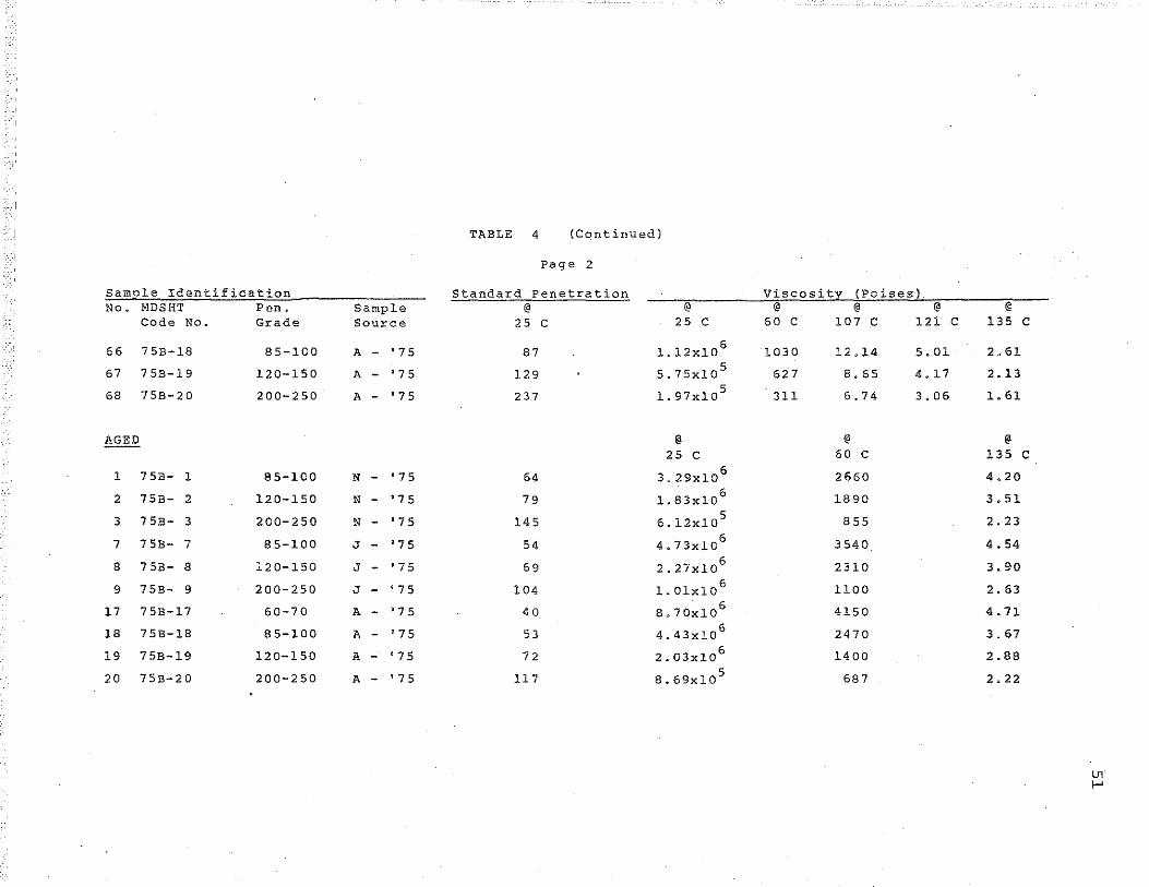
TABLE 4 (Continued)
Page 2
SamE)e Identification Standard Penetration Viscosity (Poises) No. MDSHT Pen. Sample @ @ @ @ @ @
Code No. Grade Source 25 c 25 c 60 c 107 c 121 c 135 c
66 75B-18 85-100 A - '75 87 1.12x10⁶ 1030 12.14 5.01 2.61
67 7 5B-19 120-150 A - '75 129 5.75x1o 5 627 8. 65 4.17 2.13
68 75B-20 200-250 A - '75 237 1.97x1o5 311 6.74 3.06 l. 61
AGED @ @ @
25 c 60 c 135 c 1 75B- 1 85-100 '75 64 6 2660 4.20 N - 3.29x10
2 75B- 2 120-150 N • 7 5 79 6 1890 3. 51 - l. 83xl0
3 75B- 3 200-250 N '7 5 14 5 5 855 2.23 - 6.12x10
7 7 5B- 7 85-100 J '75 54 6 3540 4. 54 - 4.73xl0
8 7 5B- 8 120-150 J - '75 69 2.27x10⁶ 2310 3.90
9 75B- 9 200-250 J - '75 104 l. Olx10 6 1100 2.63
17 75B-17 60-70 A - '75 40 8.70xl0 6 4150 4.71
18 75B-18 85-100 A - '75 53 4.43xlo 6 2470 3. 67
19 7 5B-19 120-150 A - '75 72 2.03x10 6 1400 2.88
20 75B-20 200-250 A - '75 117 8.69xlo 5 687 2.22
- -- - --
52
TABLE 5
DIFFERENCES BETWEEN AGED VISCOSITY AND ORIGINAL VISCOSITY
samr1e Log: Log: Aged Viscosity - Log: Log: Original Viscosity NO. @ @ @
25 c 60 c 135 c
75B - 1 .032 . 028 .027
75B - 2 • 031 .030 • 02 6
7 5B - 3 . 03 7 . 033 .027
75B - 4 • 038 .033 .031
7 5B - 5 .037 . 034 .028
75B - 6 . 034 . 0 2 4
75B - 7 • 03 3 . 0 3 6 • 017
75B - 8 .034 . Q39 . 028
75B - 9 .035 .q36 . 02 7
75B - 13 .030 .Q30 .025
75B - 14 • 019 . 03 2 .020
75B - 15 .030 . 018 ,025
75B - 16 . 02 9 .036 .030
75B - 17 .029 .032 .027
7 58 - 18 .031 .032 • 02 6
7 58 - 19 .030 . 031 .023
7 SB - 20 • 03 7 .032 • 0 2 7
7 58 - 24 • 02 8 • 024
758 - 25 .030 .037 • 031
7 58 - 26 . 0 2 7 .026 ,016
758 - 30 .022 .018
7 58 - 31 . 017
758 - 32 . 018 . 019
7 58 - 33 • 0 2 3 .022
758 - 34 . 02 7 . 028
Average . 030 Avg • . 030 Avg • ~ .026
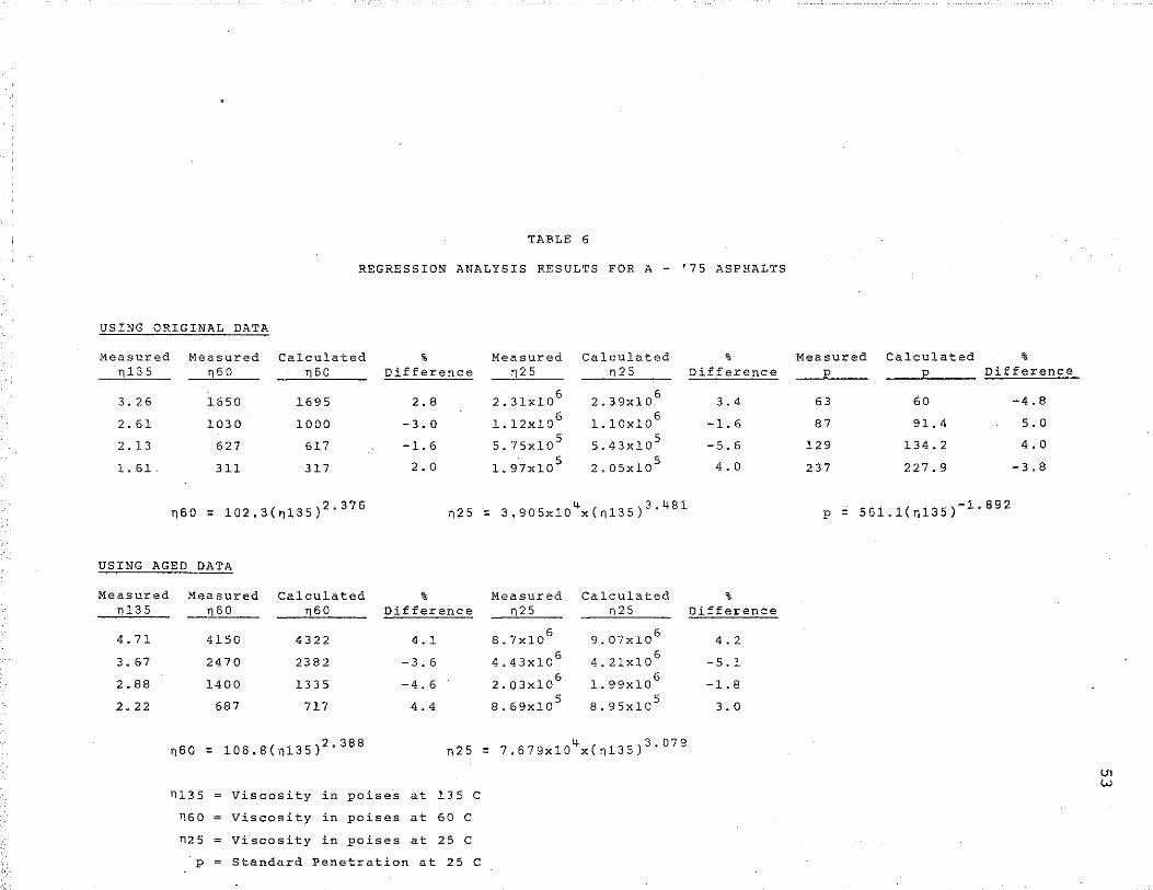
TABLE 6
REGRESSION ANALYSIS RESULTS FOR A - '75 ASPHALTS
USING ORIGINAL DATA
Measured n135
3. 26
2. 61
2.13
1. 61.
Measured n60
1650
1030
627
311
Calculated n60
1695
1000
617
317
• Difference
2. 8
-3.0
-1.6
2.0
Measured n25
2.3lxlo6
1.12x10⁶
5.75x10⁵
. 5 l. 97x10
Calculated n25
2.39x10⁶
1.10x10 6
5.43x10⁵
2.05x10⁵
n6o = 102.3(n13s)2
·376
n25 = 3.905xl04x(n135)
3•481
USING AGED DATA
Measured n135
4.71
3.67
2.88
2. 22
Measured nso
4150
2470
1400
687
Calculated n60
4322
2382
133 5
717
• Difference
4.1
-3.6
-4. 6
4.4
Measured n25
8.7x10⁶
4.43xl0 6
2.03x10 6
8.69xl05
Calculated n25
9.07xlo 6
4.2lxl06
l. 99x106
8.95xl05
n6o = 105.B(n13s)2
·388 n25 = 7.679x10
4x(n135)
3•
079
n135 Viscosity in poises at 135 C
n60 Viscosity in poises at 60 c
n25 Viscosity in poises at 25 C
p Standard Penetration at 25 C
• Difference
3.4
-1.6
-5.6
4.0
• Difference
4.2
-5.1
-1.8
3.0
Measured Calculated • Difference
63 60 -4.8
87 91.4 5.0
129 134.2 4.0
237 227.9 -3.8
p = 561.1(n135l-1
·892
U1 w
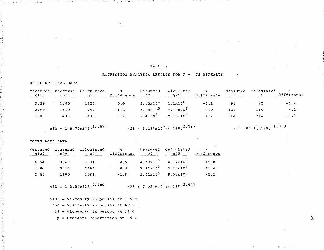
TABLE 7
REGRESSION ANALYSIS RESULTS FOR J - '75 ASPHALTS
USING ORIGINAL DATA
Measured ~135
3. 59
2. 69
l. 89
Measured ~60
1290
810
435
Calculated n50
1301
7 97
438
% Difference
0.9
-l. 6
0.7
Measured ~25
l.12xl06
5.28xla5
2.4x10 5
Calculated n25
l.lxlo6
5.49xlo5
2.36xl0 5
n50 = 148.7(n135)1
"697
n25 = 5 .134xl04x(n135)
2"
395
USING AGED DATA
~1easured
nl35
4. 54
3.90
2.63
Measured ~50
3540
2310
1100
Calculated nso
3381
2462
1081
%
f>ffference
-4.5
6.6
-1.8
Measured Calculated n25 n25
4.73x1o6 4.12xl0 6
2.27x10⁶ 2.75x10 6
1.01x1o6 9.58x10⁵
n50 = 143.3(n135) 2 "089
n25 = 7.22lxl04x(nl35)
2"
673
nl35 Viscosity in poises at 135 c
n6o Viscosity in poises at 60 c
n25 = Viscosity in poises at 25 c p Standard Penetration at 25 c
%
Difference
-2.1
4.0
-1.7
%
Difference
-12.8
21.0
-5.2
Measured Calculated % riffference
94 92 -2.2
129 134 4.2
218 214 -1.8
p = 495.1(n135)- 1 " 318
U1 ...
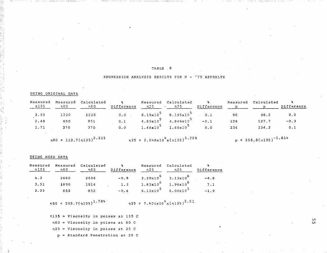
TABLE . 8
REGRESSION ANALYSIS RESULTS FOR N - '75 ASPHALTS
USING ORIGINAL DATA
Measured n135
2. 93
2.49
1. 71
Measured n60
1220
850
370
Calculated n6o
1220
851
370
%
Difference
o.o
0.1
o.o
Measured Calculated n25 n25
8.19xl0 5 8.195x10 5
4.85xl05
4.846xl0 5
1.44xl05
l.44x105
n60 = 112.7(nl35)2
" 215 n25 = 2.548x10
4x(n135)
3"
229
USING AGED DATA
Measured n13 5
4.2
3.51
2.23
Measured n60
2660
1890
855
Calculated n60
2636
1914
852
% Difference
-0.9
1.3
-0.4
Measured Calculated n25 n25
3.29x10⁶
3.13x10⁶
1. 83x106
1. 96x106
6.12x10⁵ 6.00x10
5
n60 = 203.7(n135)1
"784
n25 = 7.401xl04x(n135)
2·61
nl35 Viscosity in poises at 135 c n5o Viscosity in poises at 60 c
n25 Viscosity in poises at 25 c p Standard Penetration at 25 c
%
Difference
0.1
-0.1
o.o
%
Difference
-4.8
7.1
-1.9
Measured Calculated %
Difference
98 98.2 0.2
128 127.7 -0.3
234 234.2 0.1
p = 556.B(n135)- 1 " 614
U1 U1
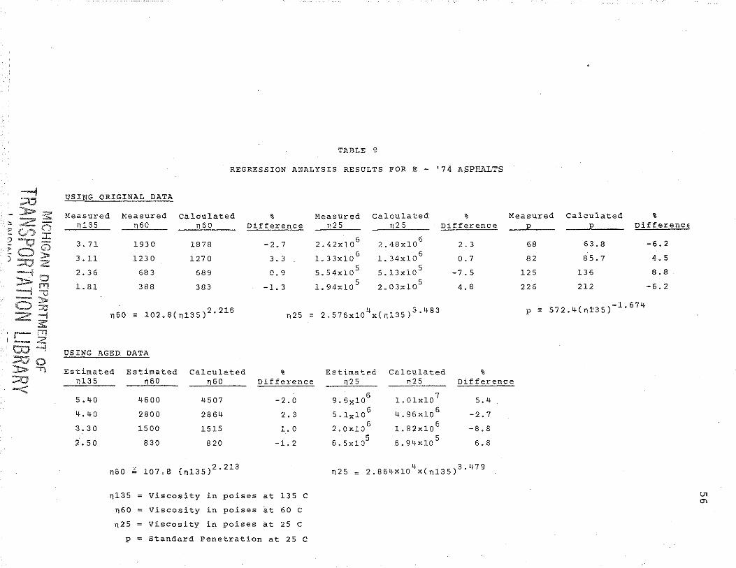
TABLE 9
REGRESSION ANALYSIS RESULTS FOR E - '74 ASPHALTS
USING ORIGINAL DATA
Measured n135
3. 71
3.11
2.36
1. 81
Measured n 60
1930
123 0
68 3
388
calculated n60
1878
127 0
689
383
n60 = 102.8(n135)2
·216
USING AGED DATA
Estimated Estimated Calculated
% Measured Difference n25
-2.7
3.3
0.9
-1. 3
2.42x1o6
1.33x1o 6
5.54xlo5
1.94xlo5
Calculated n25
6 2.48xl0
1.34xl06
5 5.13xl0
2.03xlo5
n25 = 2.576x10⁴x(nl35)
3"483
%
Difference
2.3
0. 7
-7.5
4.8
% Estimated Calculated %
Measured Calculated %
DifferencE
68 63.8 -6.2
82 85.7 4.5
125 136 8.8
226 212 -6.2
p = 572.4(n~35)- 1 " 674
nl35 n60 nso Difference n25 n25 Difference
5.40 4600 4507 -2.0 9.6xl0 6
l.Olxlo7
5.4
4.40 2800 2864 2. 3 5.lxl0 6 4.96xlo 6
-2.7
3.30 1500 1515 1.0 2.0xl0 6 1.82xlo 6 -8.8
2.50 830 820 -1.2 6.5xl0 5
6.94xlo5
6.8
n60 ~ 107.8 (nl35)2.213 4 3.479 n25 = 2.864xlO x(nl35)
nl35 Viscosity in poises at 135 c n60 = Viscosity in poises at 60 c
n25 Viscosity in poises at 25 c p = Standard Penetration at 25 c
U1
"'
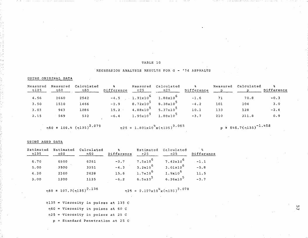
TABLE 10
REGRESSION ANALYSIS RESULTS FOR G - '74 ASPHALTS
USING ORIGINAL DATA
Measured Measured Calculated ' n135 n6o n6o Difference
4.56 2660 2542 -4.5
3. 50 1510 1466 -2.9
3. 03 943 1086 15.2
2.15 569 532 -6.4
n6o = 108.4 (n135)2.079 n25 =
USING AGED DATA
Estimated Estimated Calculated ' n135 n60 n6o Difference
6.70
5.00
4.30
3. 00
6500 6261 -3.7
3 500 3351 -4. 3
2100 2428 15.6
1200 1125 -6.2
n60 = 107.7(n135)2
·136
nl35
n6o
Viscosity in poises at 135 C
Viscosity in poises at 60 C
n25 Viscdsity in poises at 25 C
p Standard Penetration at 25 C
Measured Calculated % Measured Calculated %
n2S n2S Difference Difference
l.91x10 6
l. 88x106
-1.6 71 70.8 -0.3
8.72xl05
8.3Bxl0 5 -4.2 101 104 3.0
4.88x10 5 5.37x1o 5
10.1 133 128 -3.4
1.95xl0 5
l.88x105
-3. 7 210 211.8 0.9
1.801xl04x(n135)
3" 063 p = 646.7(n135)-1 "458
Estimated Calculated %
n25 n2S Difference
7.5x10⁶
7.42x10 6 -1.1
3.2x10⁶
3.01x10⁶
-5.8
1. 7x10 6 l.9xl0
6 11.5
6.5x10⁵
6.26x10⁵
-3.7
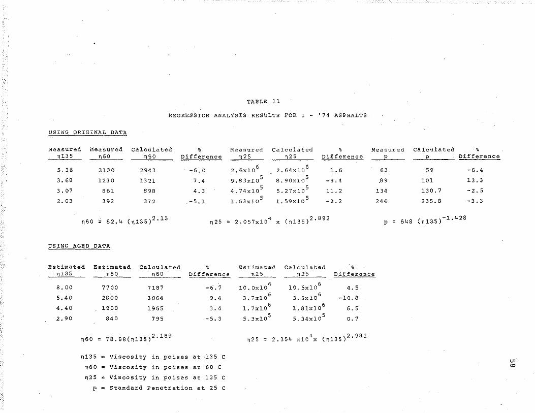
TABLE .11
REGRESSION ANALYSIS RESULTS FOR I - '74 ASPHALTS
USING ORIGINAL DATA
Measured Measured Calculated % Measured Calculated % Measured n135 n60 n5o Difference n25 n25 Difference
5. 3 6 3130 2943 -6.0 2.6xl0 6
2.64x10 6
1.6 63
3. 68 1230 1321 7.4 9.83x10⁵
8.90x10 5
-9.4 .89
3,07 861 898 4. 3 4.74x10⁵
5.27x10⁵
11.2 134
2. 03 392 372 -5.1 l.63xl05
l. 59x105
-2.2 244
n60 = 82.4 (n135)2.13 n25 = 2.057x10 4 (n135)2.B92 X p = 648
USING AGED DATA
Estimated Estimated Calculated • Estimated Calculated • n135 n60 n 50 Difference n25 n25 Difference
8.00 7700 7187 -6.7 10.0x10 6
10.5x10 6
4.5
5. 40 2800 3 064 9.4 3.7x10 6
3. 3xl06
-10.8
4.40 1900 1965 3. 4 1.7x10 6
l.81x106
6.5
2.90 840 795 -5. 3 5.3x10 5 5.34x10
5 0.7
n60 = 78.9B(n13S)2
'169 4 2.931
n25 = 2.354 xlO x (n135)
nl35 Viscosity in poises at 135 c n6o Viscosity in poises at 60 c n25 Viscosity in poises at 135 c
p Standard Penetration at 25 c
Calculated • Difference
59 -6.4
101 13.3
130.7 -2,5
235.8 -3.3
(n135)-1.428
U1 00
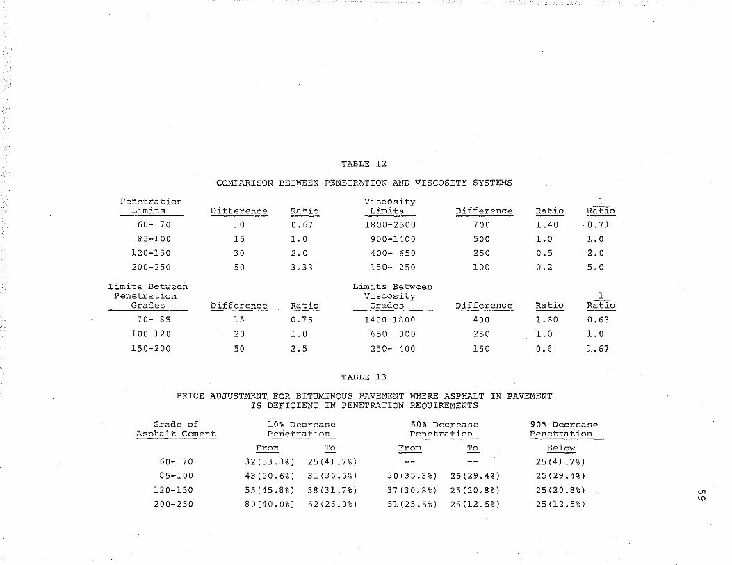
TABLE 12
COMPARISON BETWEEN PENETRATION AND VISCOSITY SYSTEMS
Penetration Viscosity 1 Limits Difference Ratio Limits Difference Ratio Ratio
60- 70 10 0.67 1800-2500 700 1.40 0.71
85-100 15 1.0 900-1400 500 1.0 1.0
120-150 30 2.0 400- 650 250 0.5 2.0
200-250 50 3.33 150- 250 100 0.2 5.0
Limits Between Limits Between Penetration Viscos-ity l
Grades Difference Ratio Grades Difference Ratio Ratio
70- 85 15 0. 7 5 1400-1800 400 1.60 0.63
100-120 20 1.0 650- 900 250 1.0 1.0
150-200 50 2.5 250- 400 150 0.6 1.67
TABLE 13
PRICE ADJUSTMENT. FOR BITUMINOUS PAVEMENT WHERE ASPHALT IN PAVEMENT IS DEFICIENT IN PENETRATION REQUIREMENTS
Grade of 10% Decrease 50% Decrease 90% Decrease ASJ2hal t Cement Perietration Penetration Penetration
From To From To Below
60- 70 32 (53 .3%) 25(41.7%) 25(41.7%)
85-100 43 (50.6%) 31(36.5%) 30(35.3%) 25(29.4%) 25(29.4%)
120-150 55(45.8%) 38 (31. 7%) 37 (30.8%) 25(20.8%) 25(20.8%)
200-250 80(40.0%) 52 (26.0%) 51(25.5%) 25(12.5%) 25(12.5%)
U1
"'
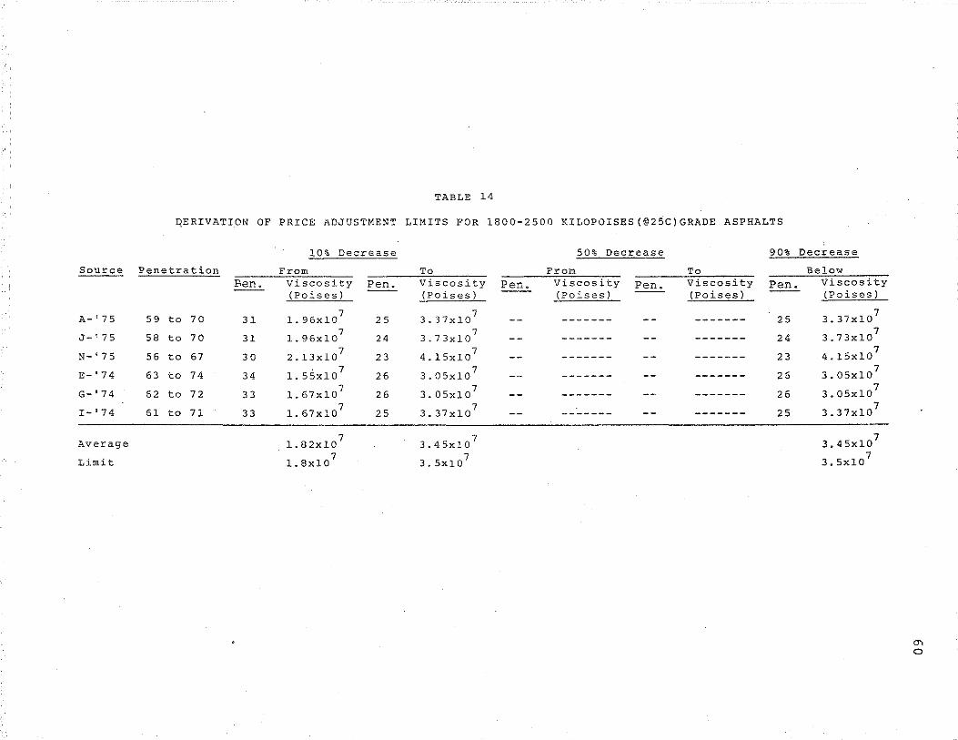
TABLE 14
QERIVATION OF PRICE ADJUSTMENT LIMITS FOR 1800-2500 KILOPOISES(@25C)GRADE ASPHALTS
10% Decrease 50% Decrease 90%
Source Penetration From To From To
~ Viscosity Pene Viscosity Pen .. Viscosity Pen .. Viscosity Pen .. (Poises) (Poises} (Poises) (Poises)
A-'75 59 to 70 31 1. 96xl0 7
25 3.37x10⁷ ------- ------- 25
J-'75 58 to 70 31 1.96xl07
24 3.73x10⁷ ------- ------- 24
N-'75 56 to 67 30 2.13x10⁷
23 4.15x10⁷ ------- ------- 23
. 7 3.05x10
7 E- 1 74 63 to 74 34 1.55xl0 26 ------- ------- 26 7
3.05x10⁷ G- 1 74 62 to 72 33 1.67x10 26 ------- ------- 26
I-'74 61 to 71 33 1.67xl07
25 3.37xl07 ------- ------- 25
Average 1.82x10 7
3.45xl07
Limit 1. 8x10 7
3. Sx 10 7
Decrease
Below Viscosity (Poises)
3.37x10 7
3.73x10 7
4.15x10 7
3.05x10 7
3.05x10 7
3.37x10 7
3.45xl0 7
3.5xl0 7
0'1 0
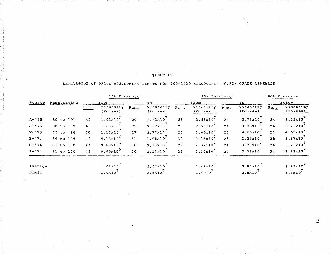
TABLE 15
DERIVATION OF PRICE ADJUSTMENT LIMITS FOR 900-1400 KILOPOISES (@25C) GRADE ASPHALTS
10% Decrease 50% Decrease 90% Decrease
Source Penetration From To From To Below Pen~ Viscosity Pen. Viscosity Pen. Viscosity Pen a
Viscosity Pen. Viscosity (Poises) (Poises) (Poises) (Poises) {Poises)
A-'75 80 to 101 40 l. 03x107
29 2.32x10 7
28 2.53xl07
24 3.73x10⁷
24 3.73x10 7
J- 1 75 80 to 102 40 1.03x10 7
29 2.32x10 7
28 2.53x10⁷
24 3.73x10⁷
24 3.73x10 7
N-'75 75 to 94 38 l.17x10 7
27 2. 77x10 7
26 3.05x10⁷
22 4.65xl0 7
22 4.65x10 7
E-'74 84 to 104 42 9.12x1o6
31 l. 96x10 7
30 2.l3x107
25 3.37x10 7
25 3.37x10 7
G-'74 81 to 100 41 9.69x10⁶
30 2.13x10 7
29 2.32x10⁷
24 3.73x10⁷
24 3.73x10 7
I- 1 74 81 to 100 41 9.69xlo6
30 2 .13x10 7
29 2.32x10 7
24 3.73x10 7
24 3.73x10 7
Average l. 01x10 7
2.27x10 7
2.48xl0 7
3.82x1o7
3.82x10 7
Limit l.Ox107
2.4xl07
2.4xl07
3.8x10⁷
3.8x10 7
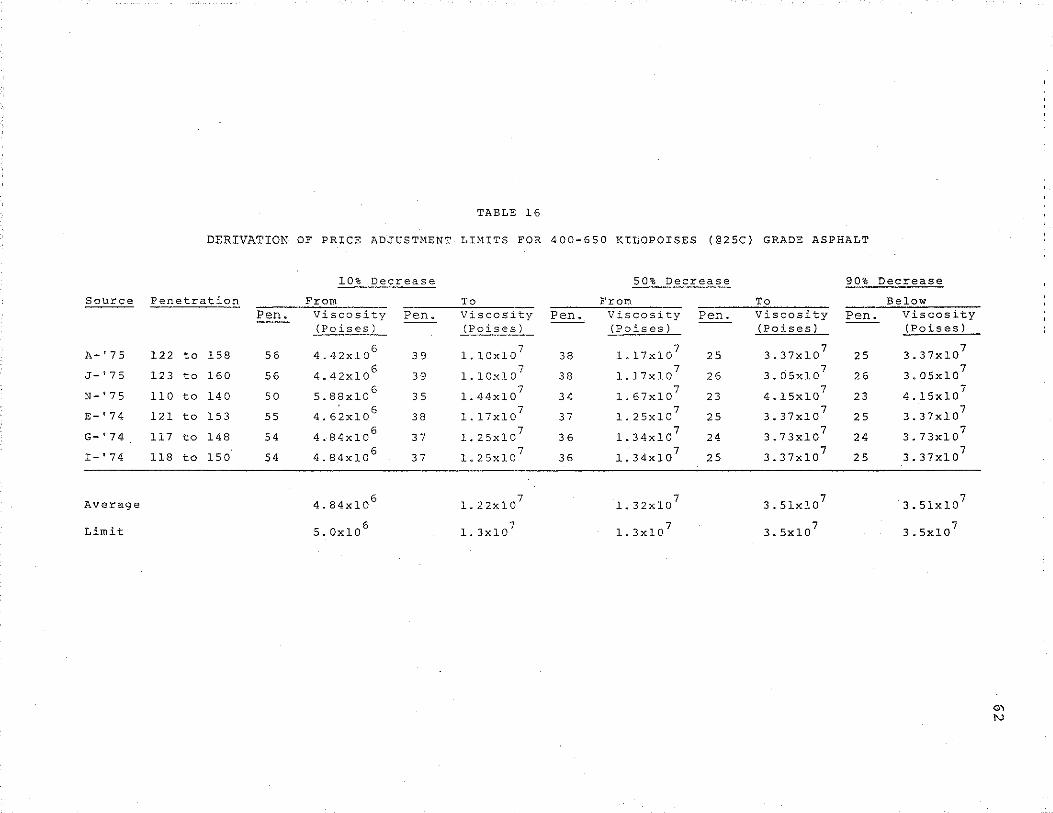
TABLE 16
DERIVATION OF PRICE ADJUSTMENT LIMITS FOR
10% Decrease
Source Penetration From To Pen. Viscosity Pen~ Viscosity
{Poises) (Poises)
A-' 7 5 122 to 158 56 4.42xlo 6 39 1.10xlo 7
6 " J-'75 123 to 160 56 4.42xl0 39 1.1o:x1o'
N-'75 110 to 140 50 5.88xlo6
35 l.44x10 7
E-'74 121 to 153 55 . 6
4.62x10 38 l.l7xl07
G-'74 117 to 148 54 4.84x10⁶
37 l.25xlo7
I-'74 118 to 150 54 4.84x10 6 37 1.25x10⁷
Average 4.84x10⁶
1.22x10⁷
Limit S.Ox106
l. 3xl 0 7
400-650 KILOPOISES (@25C)
50% Decrease
From Pen~ Viscosity Pen.
(Poises)
38 1.17x10 7
25
38 l.l7x10 7
26
34 1. 67x10 7
23
37 1.25x10⁷
25
36 1.34x10⁷
24
36 . 7
1.34x10 25
1. 32x10 7
l.3xl07
GRADE ASPHALT
90%
To Viscosity Pen. (Poises)
3.37xl07
25
3.05xl07
26
4.15xl0 7
23
3.37xl07
25
3.73xl0 7
24
3.37x10⁷
25
3.51xl07
3.5xlo7
Decrease
Below Viscosity (Poises)
3.37x10 7
3.05xl0 7
4.15x10 7
3.37xl0 7
3.73x10⁷
3.37x10 7
3.51xl0 7
3.5xl07
"' "'
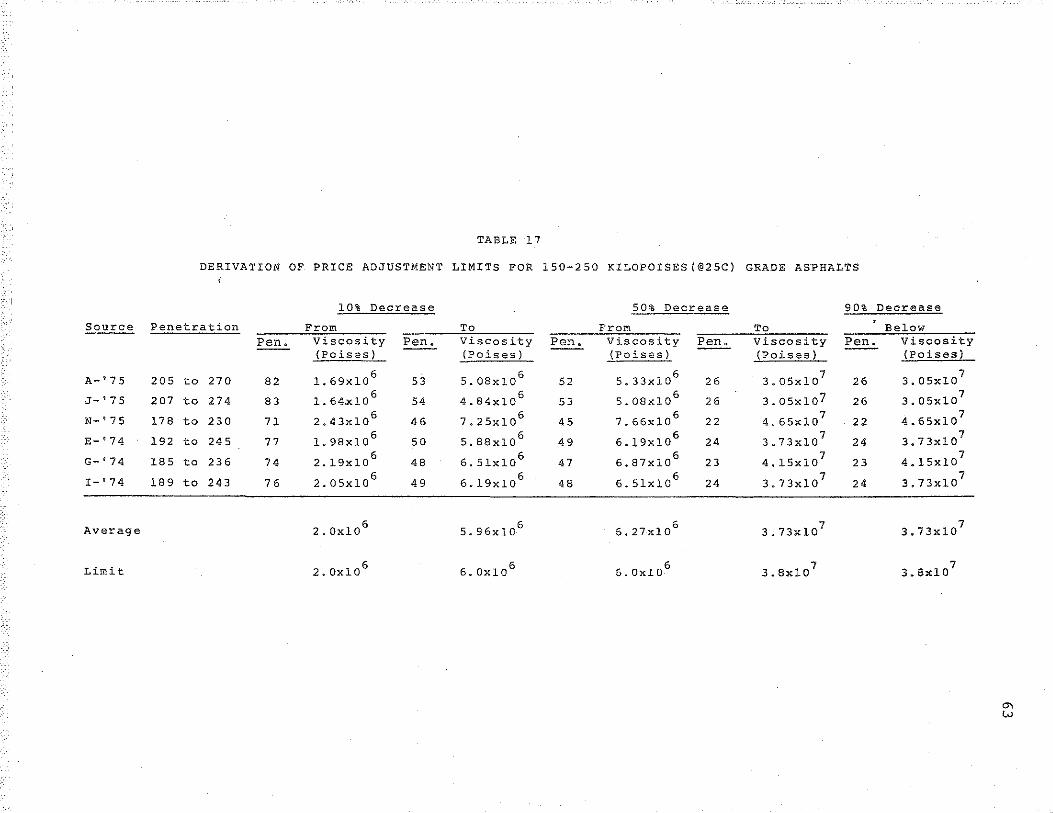
TABLE 17
DERIVATION OF PRICE ADJUSTMENT LIMITS FOR 150-250 KILOPOISES(@25C) GRADE ASPHALTS
10% Decrease 50% Decrease 90% Decrease
Source Penetration From To From To Below Pen. Viscosity Peno Viscosity Pen. Viscosity Pen .. Viscosity Pen~ Viscosity
(Poises) (Poises) (Poises) (Poises) (Poises)
A-~75 205 to 270 82 1.69x10 6
53 5.08x1o6
52 5.33x10 6
26 3.05x10 7
26 3.05x10 7
J- 1 75 207 to 274 83 1.64.:xl0 6
54 4.84x10⁶
53 5.08x10⁶
26 3.05x1o7 26 3.05x10 7
N-'75 178 to 230 71 2.43x10⁶
46 7.25x10 6 45 7.66x10
6 22 4.65xlo
7 22 4.65x10
7
E-'74 192 to 245 77 l. 98x106
50 5.88x10⁶
49 6.J.9x10 6 24 3.73x10
7 24 3.73x10
7
G-'74 185 to 236 74 2.19x10 6
48 6.51x1o6
47 6.87xl0 6
23 4.15x10 7
23 4.15xl0 7
I-'74 189 to 243 76 2.05xl06
49 6.19xl0 6
48 6.5lxl0 6
24 3.73xl0 7
24 3.73xl0 7
Average 2.0x10⁶
5. 96xl06
6.27x10 6
3. 73xl07
3.73xl0 7
Limit 2.0x10⁶
6.0x1o 6 6.0x10
6 3.Bx10
7 3.8xl0
7
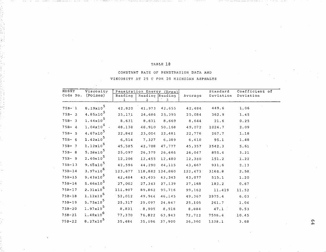
TABLE 18
CONSTANT RATE OF PENETRATION DATA AND
VISCOSITY AT 25 c FOR 28 MICHIGAN ASPHALTS
MDSHT Viscosity Penetration Energy (Era~) Standard Coefficient of ·Code No. (Poises) Reading I Reading IR.eading Average Deviation Deviation
1 2 3
75B- 1 8.19x10 5
42,820 41,973 42,655 4 2, 484 449.6 l. 06
75B- 2 4.85x10⁵
25,171 24, 68 6 25,395 2 5. 084 362.9 l. 45
75B- 3 l.44x105
8,631 8,631 8,669 8, 644 21.6 0.25
7 5B- 4 1. 04x106
48,138 48,910 50,168 4 9. 07 2 1024.7 2.09
7 SB- 5 4,67x10 5 22,842 23,004 22,481 22,776 267.7 1.18
75B- 6 l.42x1o 5 6,514 7,327 6,389 6,410 95.1 1. 48
75B- 7 1.12x10⁶
45,585 42,708 47,777 45,357 2542.3 5. 61
75B- 8 5.28x1o5
25,097 26,379 26,666 26,047 855.4 3.21
75B- 9 2~40xl0 5 12,206 12,455 12,480 12,380 151.2 1. 22
75B-13 9. 6Sx1o5
42,596 44,290 44,115 43,667 931.6 2.13
7SB-14 3.97x10⁶
123,677 118,882 124,860 122,473 3165.8 2. 58
75B-15 9.43x10⁵
42,484 43,405 43,343 43,077 515.1 l. 20
75B-16 5.46x1o 5 27,0'02 27,363 27,139 27,168 182.2 0.67
75B-17 2.31x10⁶
111,907 89,862 95,716 99,162 11.419 11.52
75B-18 l.12x106
52,012 49,944 46,145 49,367 2975.4 6.03
7 5B-19 5.75x10⁵
25,317 25,097 24,847 25,105 261.7 1.04
75B-20 l. 97x1o5
8,831 8,905 8,918 8,884 47.1 0.53
7 5B-2l 1. 48x106
77,370 76,822 63,943 72,712 7598.4 10,45
75B-22 8.27x10 5 35,484 35,696 37,900 3 6. 3 60 1338.1 3. 68 0"\
""
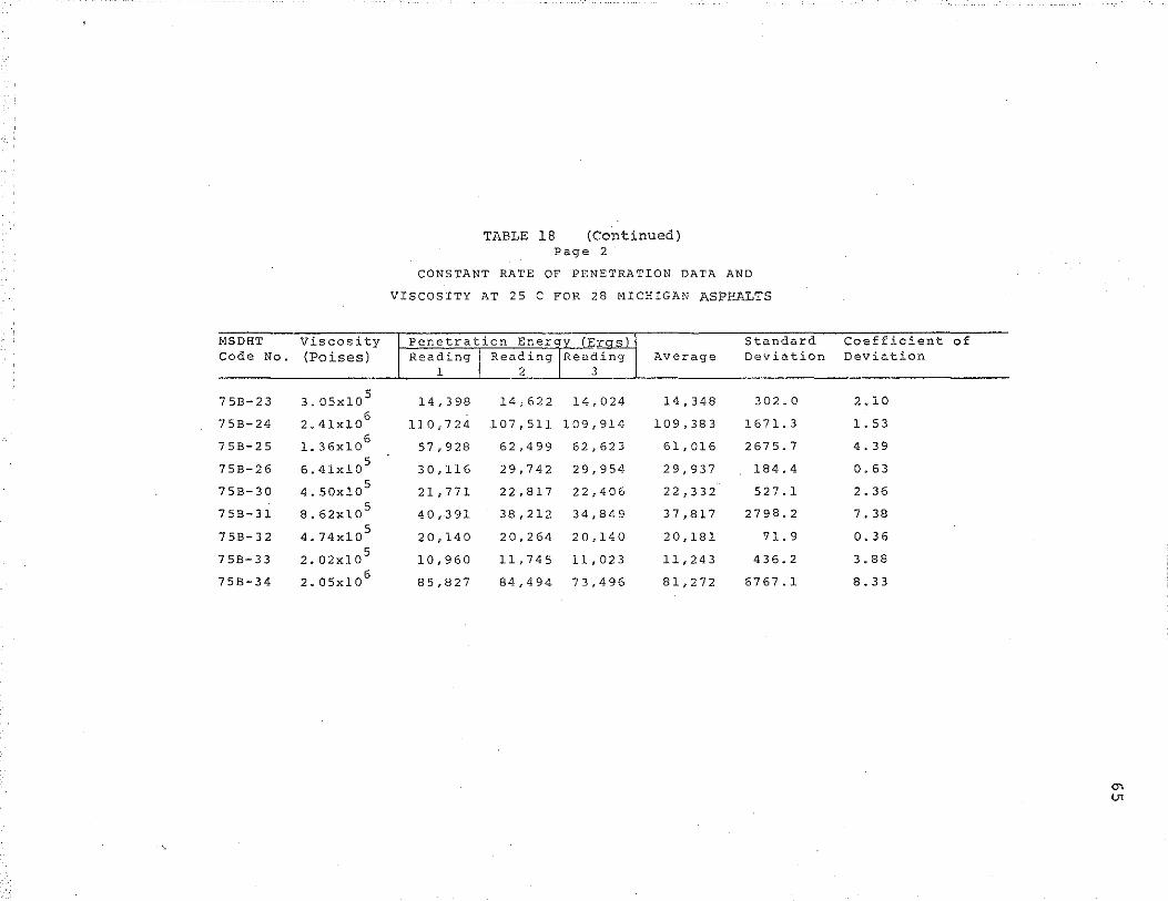
MSDHT Viscosity Code No. (Poises)
75B-23 3.05x10 5
75B-24 2.4lx10 6
75B-25 1.36x10 6
75B-26 6.4lxl0 5
75B-30 4.50xlo5
75B-31 8. 62x105
7 SB- 3 2 4.74x10⁵
75B-33 2.02x10⁵
75B-34 2.05x10⁶
TABLE 18 (Continued) Page 2
CONSTANT RATE OF PENETRATION DATA AND
VISCOSITY AT 25 c FOR 28 MICHIGAN ASPBALTS
Penetration Enerqy (~~ Standard Reading l Reading IRead.ing Average Deviation
1 2 3
14,398 14,622 14,024 14,348 302.0
110,724 107,511 109,914 109,383 1671.3
57,928 62,499 62 '62 3 61,016 2675.7
30,116 29,742 29,954 29,937 184.4
21,771 22,817 22,406 22,332 527.1
40,.391 38,212 34,849 37,817 2798.2
2 0' 14 0 2 0, 2 64 20,140 20,181 ?1. 9
10,960 11' 74 5 11,023 11,243 436.2
85,827 84 1 4 94 73,496 81,272 6767.1
Coefficient Deviation
2.10
1. 53
4.39
0.63
2.36
7. 38
0.36
3.88
8.33
of
"' U1
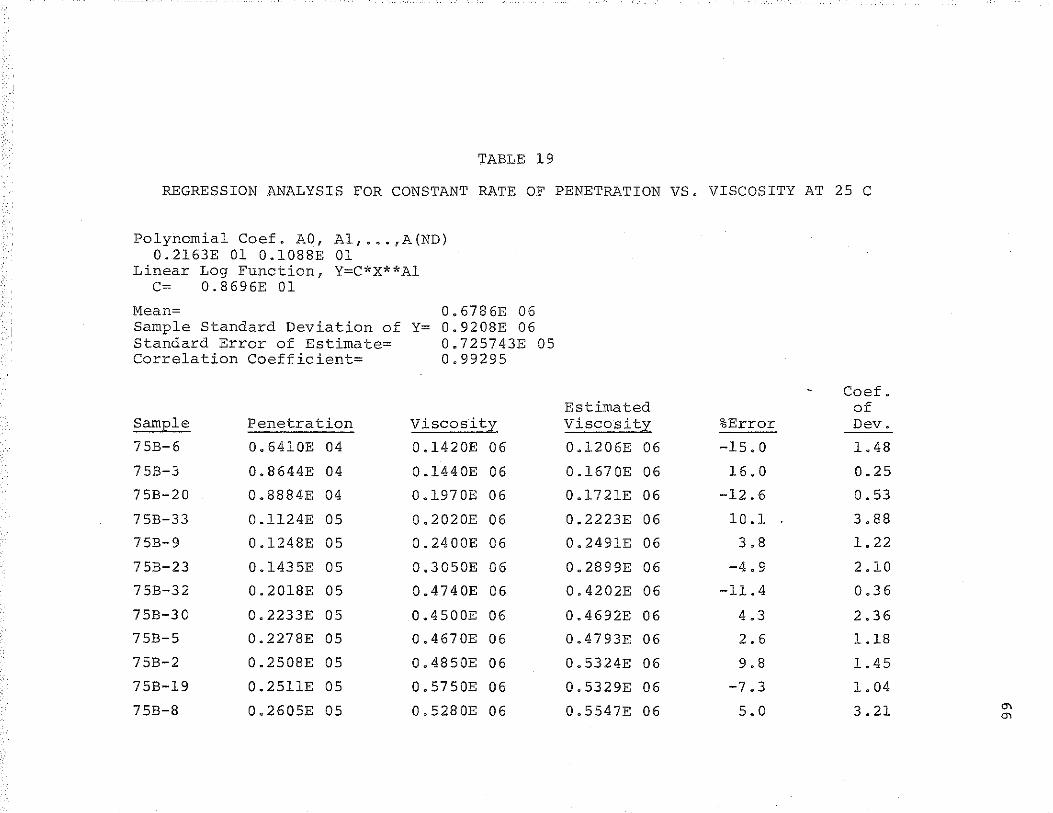
TABLE 19
REGRESSION ANALYSIS FOR CONSTANT RATE OF PENETRATION vs. VISCOSITY AT 25 c
Polynomial Coef. AD, Al, ... ,A(ND) 0.2163E 01 0.1088E 01
Linear Log Function, Y=C*X**Al C= 0. 8696E 01
Mean= 0.6786E 06 Sample Standard Deviation of Y= 0.9208E 06 Standard Error of Estimate= 0.725743E 05 Correlation Coefficient= 0.99295
Coef. Estimated of
SamEle Penetration Viscosity Viscosity %Error Dev.
75B-6 0.6410E 04 0.1420E 06 0.1206E 06 -15.0 1.48
75B-3 0.8644E 04 0.1440E 06 O.l670E 06 16.0 0.25
75B-20 0.8884E 04 0.1970E 06 0.1721E 06 -12.6 0.53
75B-33 O.ll24E 05 0.2020E 06 0.2223E 06 10.1 3.88
75B-9 0.1248E 05 0.2400E 06 0.2491E 06 3.8 1. 22
75B-23 0.1435E 05 0.3050E 06 0.2899E 06 -4.9 2.10
75B-32 0.2018E 05 0.4740E 06 0.4202E 06 -11.4 0.36
75B-30 0.2233E 05 0.4500E 06 0.4692E 06 4.3 2.36
75B-5 0.2278E 05 0.4670E 06 0.4793E 06 2. 6 1.18
75B-2 0.2508E 05 0.4850E 06 0.5324E 06 9.8 1.45
75B-19 0.25llE 05 0.5750E 06 0.5329E 06 -7.3 1.04
75B-8 0.2605E 05 0.5280E 06 0.5547E 06 5.0 3.21 0"\ 0"\
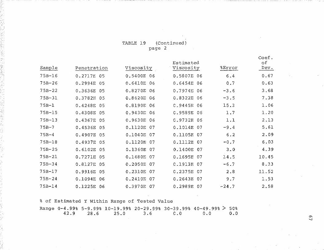
• I
TABLE 19 (Continued) page 2
Coef. Estimated of
Sample Penetration Viscosity Viscosity %Error Dev.
75B-16 0.2717E 05 0.5400E 06 0.5807E 06 6.4 0.67
75B-26 0.2994E 05 0.6410E 06 0.6454E 06 0.7 0.63
75B-22 0.3636E 05 0.8270E 06 0.7974E 06 -3.6 3.68
75B-31 0.3782E 05 0.8620E 06 0.8322E 06 -3.5 7.38
75B-l 0.4248E 05 0.8190E 06 0.9445E 06 15.3 1. 06
75B-15 0.4308E 05 0. 9430E 06 0.9589E 06 1.7 1. 20
75B-13 0.4367E 05 0.9630E 06 0.9732E 06 1.1 2.13
75B-7 0.4536E 05 0.1120E 07 O.l014E 07 -9.4 5.61
75B-4 0.4907E 05 0.1040E 07 0 .ll05E 07 6.2 2.09
75B-18 0.4937E 05 0.1120E 07 0.1112E 07 -0.7 6.03
75B-25 0.6102E 05 O.l360E 07 0.1400E 07 3.0 4.39
75B-21 0.7271E 05 O.l480E 07 0.1695E 07 14.5 10.45
75B-34 0.8127E 05 0.2050E 07 0 .1913E 07 -6.7 8.33
75B-17 0.9916E 05 0.2310E 07 0.2375E 07 2.8 11.52
75B-24 0.1094E 06 0.2410E 07 0.2643E 07 9.7 1. 53
75B-14 0.1225E 06 0.3970E 07 0.2989E 07 -24.7 2.58
% of Estimated Y Within Range of Tested Value
Range 0-4.99% 5-9.99% 10-19.99% 20-29.99% 30-39.99% 40-49.99%> 50% 42.9 28.6 25.0 3.6 0.0 0.0 0.0
"' "
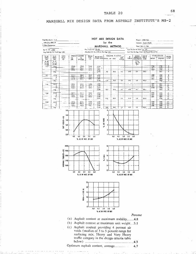
TABLE 20
MARSHALL MIX DESIGN DATA FROM ASPHALT INSTITUTE'S MS-2
HOT MIX DESIGN DATA by the
MARSHALL METHOD
l'rojo<t: F-003-4(2)
i\og_ 1\~lk Sp. Gr. Tot•lllgg. 2_e_, ___ _
• ' 1
1
160
15 9
100
~ 190
5 180
0
0
0
~ 0 f"
~'" 0
/ ~ I
4.0 4.5 5.0 5.5 6.0
% AC BY WGt Of MIX
/ \ \
\ \
4.(} 4.5 s.o 5.5 6.0 "'o AC SY WGT. Of MIX
' 0
' 0
,....-'
8
1
' ' • '
/
4.0 4j s.o 5.5 6.0
% AC DY WGT. Of MIX
I i i /
...... /
4.0 4.5 5.0 s.s 6.0
% AC BY WGl Of MIX
4.0 4.5 5.0 5.5 6.0
% AC BY WGt Of MIX
Percent (a) Asphalt content at maximum stability_ ..4.8 (b) Asphalt content at maximum unit weight .. .5.1 (c) Asphalt content providing 4 percent air
voids (median of 3 to 5 percent range for surfacing mix, Heavy and Very Heavy traffic category in the design criteria table below) _____________ .. .4.3
Optimum asphalt content, average ............. _. _____ _4,7
68
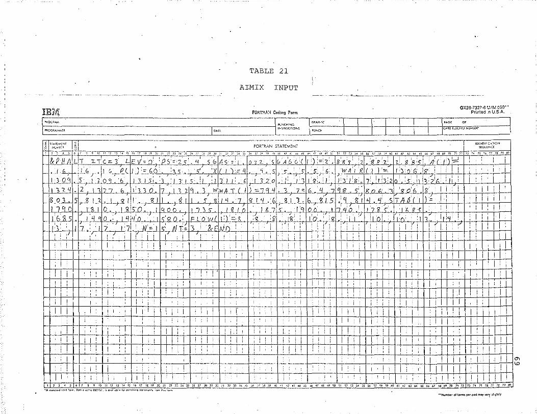
TABLE 21
AIMIX INPUT
IBM FORTRAN Coding Form
LP~OG~AM ~ I"UNO<ING
PROGRAMMER I OAr< IINSIRUCliONS
i ';IATl>hONI
8 FORTRAN STATEMENT 8 NU'·~n 0
' ' ' ' ' ' ' ' " "l) 1) ,. , 16 17 li) 19 1\l 11 '~ 7] 1< .•5 -:~ 17 ~a /? JU J I J.' J1 "' 1\ " ]/ }~ "\? -1<1 ,, <7 '' ... ,
&fHA. L.l 'IT c-3 L ,CC f. v'='o' rJs=z,- . y' 's G lAs:=' I: In 221 'I G'A'b (,i(
I G: ~6,Q lr11.:=1 I,(, c,;._£1- s35c... ~,..'.;x r,."',.~ t~.s ;.s::-~,3:
=~.1 fL'- "
I :}.0'\ 0.3... 6 ~ _1_3, 1 ~s.i._ 3.+-LJ.l s..J.tc,.i ' ' ' ,"L3'lo "'--~J~.-~1~ J~LJ..'..:J 1'1,?.4 • 2 1 o 2..7 ... .b"f' cil3..0 .. L 4L1.2 j' } w WitT ( I l ""7 'L':I ,_]_~
' S OJ~ I 11 I ~~ T"·u L._rZI I 5 .-\l. ..L.':L.~:Z, 'LL':L .• ~b s: ,_3'__1_1 .,_E..Ll.~ I 7 '1C 0. I 11 I II l '>.Q.. I lq O..Q.,_ ,,,, I.~LO ~~L7 I 'q
' :I·~ o 'iii '·t l}.=::~L 5...(_;·-·
..1)>.'3.5 .o_..,.~ p:S:.~ £..LQ.Ild rL- g : ' i '
r- ~-,J.<L .• .c • : {! ·~-,.,: ; 7 '' 7 ., .-, ~~~ 3 &E Ni ' : i : i I ! ' :' ' 57 .N - I.L;.-- ~~
' ! ,} / ~ : ' ·i-:-,-~-~ I i 1 I I ' ! i ! : : ' ' I ' ·: i I : ' I ' ' ~.
' i I : I i ' i I i : I • I I ' ! i I i i ' I
i ' i : ' i : I ' ! I I ' ~· : I ' I I I I
' ' '
! ' i I I I ! ' ' I i ' i
' ' I ' ! I I
t i I ' ' ' I i I ' I i : ' : : ' I I ' I ' I I I I ! ! I i I I ! ' '
' ' ' ' ' '
i
! I ' ' ' I : I ' !
' ' I I : ' I ! ' I I ' I i i ' ! ' '
I I
I i i ' i ! ' I i ' I : i I ' i ! ; i ' I ' ' '
I
' ' ' ' ' ! I ' ' ' ' ' ' i ' '
i I I '
I I I I i i : i
' I
I I I i i I ' I i : ~~ I : I i i r ! ' ' I i ! ' ' I ·, ' ' I I
I i I ' ' ' i I ' I ! I I I ' ' ' '
I : I ' ' I I .; I ' I I ! I I i i I ' I ' I ! ' I ! ' ' I ' ' '' ! : ' ' '
I : I I I i ! ' ' i ' i I I I ! I I I ' I I I : I I i ' I i ' I I i i ' ' I I I I ' I I
I I ' ' ' ' i I I I ! I I ' : ' ' ' ' I ' i ' I ! I
i ' i i ' I I I I ' ' ' I ! ' ' I i I ' I
'
! ·. I i ' I ' I · I ! I !
' : :
I I I I I I ! : I , I I ' : ' ' ' ' '
' ' ' . ' • ' • ' '" II 11 n ~~ 15 I~ 17 IB 19" 2<l ?I n n <• <5 16 u 7e :;>9 JO jJ 31 3.1 ·~ J; ~~ V '!S J9 . " <7 jJ 4.;\ <';
•A .,,..J~,d co•~ '"""• IOM el~"o 0~61~1. i• ovo;lo±or~ lot"""<!""~ ""'""'""'' '""" ''"' to,.,
~ G~AP!;IC
II'I.)NCH
·~ <7 '" ,., sa
.0 :::;;:z;. ':' : ~: !'9; I 1: .L4 :.,
(u. G~. o o' 1
I'll: : e ! i ( l ' ' '
' ' I . I ~ ·~ I
~
' ' I ' i '
I
i i ! i I I
I ' ' ' I ' I
i I I I
I I ' I i ' !
\ ' ' ! ' I
' i
i ' I I : I f i ! : ' ' i
. '
: '
'
I I I I ! I I I I I
I I I I
PACE
GX28-7327-6 U/M oso· • Printed ln U.S.A.
oe J C.<.~O El!<CTRO NUMB<R•
ID!;NTIFIC"tiQN SEQUENCE
" 5? 5J 5< 55 56 vs~>•60ol " hl " 65 M 67 oa 69 70 71 77 !J 7< 75 ?6 77 ~~ )Q so
z's',· 1 2 ' ' I : <.!. & 's:, _'tiLC_II) i:=J I I '
' I i 8 !1 2' I
WA'I R ! I I l : ,:) 0 !L. r, ' i I 1 ' i I i 52 ! I ' I I I I
1'3~ JlJlJ3 12 I r : 1
1-, 21 6! : lr I i I I I lo 5 CL ' r. '! I I I I q s .~s_;. IFr" "'' ,, '<? o'6 3:_' I i : i i
l'l~'L s t . I ' I i ' I I ' g T If 6 II )= ,1 ' I I .:.:L .. 'I ' ' '
]'Lin ' 117 g ,, I I. !1 I' I i I ' ' ' ' I I I ' I '
1 I l ' i1o! I:(): ' I I l' I I, l'l ' I ' I i I I ' '
";j:' :i I I IT' ' I I I i ' I ( I I I I I I I I ' , I ' I ' ' ' ' i I i i I I I I I I I ! I I ' : i :
I ! I I, i ! I i I I I I I i I I I I I I
I ' i i I I I I ! I I I ' I I I I i I I I ' ' I I ' ! I ' I I ' : ! I I ' i I I I I ! I
' I ' 1 ! I
' I I I IJ ' I I I ! I I I I I I I I ' I I I I
I ' ' ' I ! I I I I
I ' '
i ! I I I I I ' I !
! 1 I ' ' i _ _I i i i I i I I I I : I I i I ' ' ' ' ' ' '
! i I i I i I i I I i I I i I ! I I I I I i ' I ! I I I I I I l I I II I I I ' I I I I I ' I I ! I I i I I I ! I ! I I ! ! I I I I I I I I
' ' i
i I I I ! ! I I I I I ! I I I ! I I I I ' I I I I I I i i ' I I I ' I I I I I I j I I I ! I ' ' i I ' i ! : . I , I I I i I I ! : ! I ' I I ' ! I ! i I ' ' ' I
' ! I I ' i : ! ! i i i I i i i ! I I i : ! I
I ! ! i ' I I I I I I I I i I i I '
: ' ' ' l j i I I I I I I I ! I ! I ~ ., •s 49 so Sl n SJ s~ ss S6 S7 58 S9 6Q 61 o1 631>44561>67 oa o9 7ll 71 71 7J 7• 757~n;g79BO
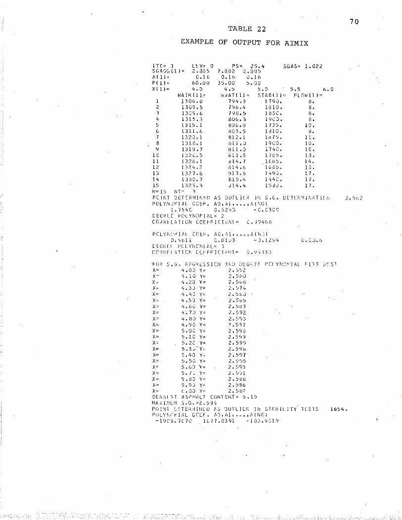
TABLE 22
EXAMPLE OF OUTPUT FOR AIMIX
I TC= J SGAGG(l l= A { 11 = P{ ll = X { 11=
LEV= 0 2. ua; c .1 6
60.00 4.0
WA!R{11.= 1 130&.8 2 1309.5 3 13GS~ 6 4 1315.3 5 131~.1 6 1311./c 7 1320.1 8 1318.1 9 1313.7
lC 132C.5 11 1326.1 12 1324.2 u 1327.6 14 13>0.7 15 1329.3 N=15 NT= 3
PS= 25~ '* ? .. 882 2.335
0.16 0 .. 16 35.00 5~GO
4 .. 5 5.0
SGAS= 1.022
5.5 w.;AT{1J= STAB!ll= FL0\1(11=
794.3 1790. u. 796.4 18 10. 8. 7'}8.5 185C~ 8. 806.3 l9C0& 8. U'J6.3 1735. l ·:) ~ 80.3~5 ldlO. u. 812 .[ ld'/S. 11 • U11.J 19CO. 10. 811 .. :} 1740. 1 c. bll.5 17U~ .. 13. 01". 7 1GB5. 14. 814.6 l6tl~. 13. 813.6 149·.1. 17. 815,/t 1.'14 0. 1 7 • d14.4 15UJ. 17.
70
6.0
PCJ~T DET~RMI~~O
PCILYNC.::/11 PL CCH-. AS CJUTLlCR li'i S. G. or-E:r· ~~. 1 1\t, T ll;'< 2, :H1Z Ao,,u, ••• ,At\LJl
l.i54S G.32J~ -C~C3CS CEGR[[ ~CLYND~Ihl= 2 CDKKf:L;UICN CCEI-FICI:::I\T= C.. 1?460
PCLYI\L·;..!JAL CCEF. AC,,'Il, .... ,t.tN~) O.S6ll Q.81J3 -J.l2:•Jt1
CEGkll PCLYNCMJhl= ) CPRR[L~TlC~ CC[FFICl~Nl= 0.Y~J3J
·~uR S.G~ R~GkESSlCN
X= 4.0.:J Y= Xc= '1. 1 U '¥= X= 4.20 Y= X= X= X= X= X= X= X= Xo X= X= x~
X= X= X= X= X= X=
<1. 3 j Y= li • 1-18 Y= 4. 5 J Y= 4.60 Y= li;.? J Y= 4.H·J Y= Lj.90 Y= 5. OJ Y= ? o t G Y= 5. 2 C Y= 5.3J.Y= 5 .'t-0 Y= !:J .. SC Y= 5.6:) Y= 5. n Y= 5 .. 80 Y= 5o 9J Y=
3HJ Df::Gi=.Cf 2.~~2 2.560 2.5u8 2. '::> 7 't 2.5bC 2.5u5 z.sH~
2.~92 2.~:<;:;
2.5S7 2.5':Jd 2. 54'=J 2.599 2.59'.) 2.597 2. ~,'15 2. 593 2. ~'j 1 .z.~~i:.)
2. 586 X= OE~O>LST MAX. I.'·lU.'-1
C. 00 Y= 2. 5 82 ~S~HALT CONTENT= '.J.l5 S.G.-""2.59',
C.CJvb
PUI:'n LfTEf~,'\lNtD f,S 'JUTLIER IN STM>ILITY. 1TSTS PULYh~~IAL CC[F. ~J,~l, ••• ,A(I~Cl
-L9C3.7C7C lL77.0391 -1U3.9Cl9
1854.
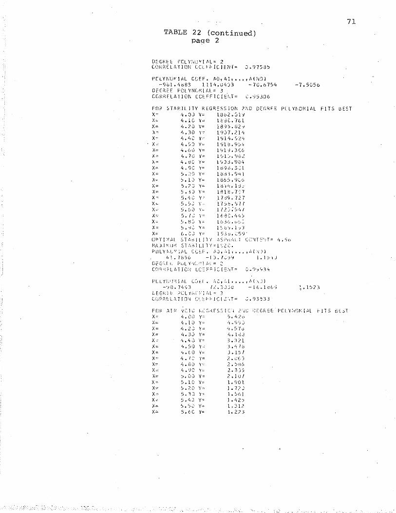
TABLE 22 (continued) paqe 2
DEGREE FCLY~uwr~L= 2 CORRELATION tC~FFICIENT= 0.97SU5
P(LYf'<Oiv'lAL CCEF. AO,tdt~H,A{,~;:ll
-9bl.4d83 1114.04)3 -70.67~4 DECREE PCLYNLMlAL= 3 CGRRELATIO~ CCEFFIC!E~T· C.~53D6
71
-7.50?6
FO~ STABILITY REGRESSION 2~C DEGREE PlLY~.OMIAL FITS BEST X= 4.0J Y= l862.Jl'i X= 4~1C Y= UL3C.-Jt..l X= 4.20 \'= 1895.82'1 X• 4.30 Y• !9)7.214 X= 4b4C Y= l9l4e!J24 X= 4.5J Y= 1SlU~9j4
x~ 4.6J Y= 1Yl~.3C6
X= 4.70 Y= 1Slj.9d2 X= 4.dC Y= l~Jd.984
X= 4.9C Y= liJ'i0.3::1 X= S.J·J Y= l0d3.94l X= ~.lJ Y= 1865.9\.G X= 5.2~ Y= lci~<t.ld:)
X= 5.3J v~ 1818.7·:'7 X-= 5.9•: Y-~ .l7J'J.727 X= 5.iJJ Y""' 11:J6.{df X;:, ~.6J Y= l72.::;<.;ttf X= 5. /:.J Y=.: l£_·8:. 1t4~
X= :-.a:; Y= 1636.'-'l'..-X= ?.~.:, Y= l;.;b'-,.1:;'3 X; 6.C.J Y= 1'.-'.:'.u.~S'J·
UPTI'>~il.L STAD!Lll"{ i'l$1-'ru\Ll CC\Hf::''!T= r,.5o F:AXJ-~·.u,~ STf\~lLI TY=l<Jzc. POLYhL'1 JAL CC.~f. AJ,4l,~ •• ,A(;"))
fJl~7856 -1::).7·>)'::1 l.l~·';J
DEGt:..LL r~t...LY·'IL:'!l /•L= 2 COR~~LATIOI~ LC~F~ICI~~T= 0.9~~34
PCLY1"<'''-',J,'IL CC1t.r-. :~c,.·.r, ... ,/,(.\'.)) -':~D~ 7'tiJ3 7?.3:J:..G ;-l6.lu60
U:GiZH: PLLYid!!Jfllo' 3 CGPRlL~TIO:~ C~~~FICI~\T= ~.93533
FOR !1. I f! vc I~~ hL C><.fS:J I .. • 2. ll~ •JlGRf:[ PCL Yi~m·. I ill ..
X• 't. co Y• '>. 4 Zl1 X= 4. I 0 Y~ ·LSSJ X• ,, • 2,:: Y• 1t. 57-J X• L1 ~ 3 J Y• <i. 1 d3 X• 4 • !; J. Y• 3. ~~ (' 1 X• 4.~0 Y" 3. 4 7 B X• <1o tO yo J. 15 l X• I; o 7 2 Y• 2. 0()
X• 4oBJ Y• 2. ~116 X• 4.9G Y• 2~33:)
X• s.oJ Y= 2 • I 0 7 X• S.lO Y~ 1. 90 l X• ~.20 yo [. 72J X• 5.3J Y= l. ~61 X• 5 ,I; J Y• L 1t2j
X• ~.?J yo !. 312 X" 5.6C Y= 1. 22 3
I-ITS 8 f: :::i 1
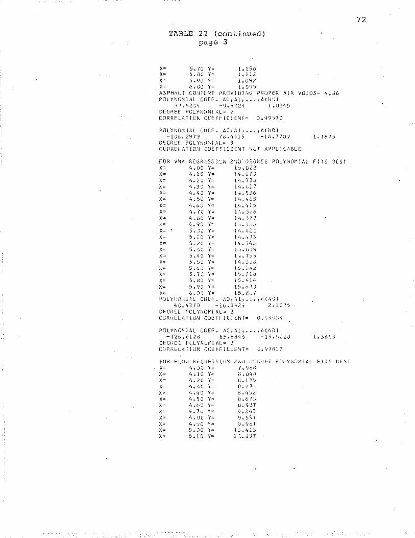
TABLE 22 (continued) page 3
X= 5Q70 Y= 1~156 X" <,,HOY= 1.112 X= 5o 90 Y= l. 092 X= 6o00 Y= 1o095 ASPHALT CO~TENT PROVIDING PROPER A[R VOIDS= 4o36 POLYNO~IAL COEF. A0 1 Al, ••• ,A(NC)
37.S2C4 -9oBZ24 1.0245 DEGREE PCLYNUHl;\l-= 2 CORRELATIO~ CCEFFlCIENT= 0~99370
POLYNQ;\ji/I.L CfJE:F. AOtAl, ••• ,A( NO) -106.2979 7cl.4%15 -16.7709 L lU25
OECREf PCLYNOMIAL= 3 CGRRELATJON CUEFFlClENT NQT APPLILAOLE
FOR V!<,, X=
REGRESSJCN Z'~J.OEG~EE POLY~O~IAL FITS BEST
X= X" X= x= x~
X" x= X= x= X= X= X=
X= X= X= X= PGL'YH
4 OEGRE
't.OO Y=- 1'..1.022 4.lc v~ 14.ci7J 4&2) Y::::. 14.730 4.30 Y= l4.L27 4.4J Y= 1~.536
4.5C Y= llt.'t65 4.60 Y= 14.41:) 4.7C Y= 1',.:3d6 4.00 Y= 1"1.3"17 4.90 Y= 14.3~d
5.JU Y= l't.4.2J 5.10 Y= 14.~73
5. 2 0 Y= 5. 3 0 Y=-5o 4 0 Y= 5.5) Y=
l 1;.j4h
l '-1. 63=1 li-.Ei3
:.>.OJ ·,·= l).l_.<t2 5.7V Y= 1').2ld 5. 8 J Y= l S ~ 4 l tt 5.'1J Y::: 1?~03)
6.JJ Y== 15~2:07
~lAL CIJE~. AO,~l, ••• ,A(NO) 9-4310 -16.5-iZ,·t 2~1C75
PCLYI,UIAL~ 2 CCRRE ~TlUN COEFFICIENT= O.S9954
POLYt\l:IIIJAL CCEF3 /IJ 1 ld, ••• ,Jdi\Jl -126~612d 85.6346 -18.5010
CEGRE~ PCLY~U~IAL= 3 CURRELATJON CCEFFJCIENT= ~.97dJ3
FOR FUJI/ REGKf::)SIO'\ n .. u u:::G~:E[ PULYi'i:J,\1 IAL X= 4 0 J,J v~ (.96d x~ 4. l 0 Y= a. o.; J X= 4.2C Y= b. 135 X= 4.3C Y= l:l.273 X= 4 o4 a Y= o. 't :>z X= 1+ • 5 Q Y= u.67:J X= 4,6J Y= tl. SJ 7 X= 4.7C Y= 9.2tt3 x= 1-J • u c Y= 9. 5 s 1 X= tt.'JO Y= 9.9Hl x~ ~ • ·JO Y= 1~,.415
X= 5o10 Y= l':oddl
1o36S3
FITS BC S T
72
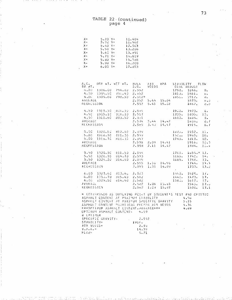
X= X= X= X= X= X= X= X= X=
TABLE 22 (continued) page 4
5QZCI Y-= llo40 1t
5 ~ "!-C Y= 11. SG2 ~ 0 '10 Y= l2oSL3 5 ~ :) G Y= 1:3.206 5. (J J Y= 13. oSil 5. 70 Y= l-1~619
s.eo Y= l:J.3d8 5.90 Y= l6.2CO 6.00 Y= 17.053
A.Co DRY hl. kET ~T. BULK Ali~ VMA GY WT. ~.JJ l306.LO 7S4.BJ 4.00 lJ09.0C 706.40 4.00 1309.60 790~5J
I-IVH·,I'IGE REGI.:..CSSJON
'<.50 1315.30 4.5C l315.1G 4.50 1311.60
AVtRt.:.Gf: REG~~f:SSICJ''!
S.8C l320,lC 5.00 LHiLJO 5.00 l3ltl.1C
t>VlRAG[ REGPESS 10!~
s.~o 132o.so 5.'JJ 1326.1.0 5~50 1324.20
AVE:f::hGE: KEGK!:SS It:~l
i;(:(,.J . .J :J C:t:. 3 J 803.5;)
ij 1 2. l.J
dll.JJ
2lL:-d t.\l4 .. 7J OlLJ.,6J
S.G. VOIDS 2.~52
2.:.')2
2. :i':J2 ~.,.4 15.0't 2.552 ::...'-t3 15.V2
2.5d4 2. ') [j 7 2. 5 t•l 2. 5 dlt 2. 5c?
2. '59') 2. 5 'i')
2. ::iS 1 2.5'10 2 .. 598
2. 5 '?<~ 2 .. 593 z .. S'J9 2.5'7~ 2.51f'5
3 .'1 {~ 3. •i ,;
2. J<)
2. 11
L 50 1. J 1
14. 't2 llt,it?
6,()) L327.C;C Bl3o6i:. 2. 5CJ 6 .. 00 1J3.J. 70 JlS.4J 2. Sll2 6.GC l329.~C 814.48 2.~d2
f,V f:R:~(;L REGRE' . .SSICN
z.~.)(i2 t.G6 t:.;.b3 2.5b2 l.C~ l~.J7
73
STililiLJTY FLOW Cl1~l i\DJUST
l"f<JJ. 1846. H. 181J. lB6L u. lH;;G. 191"2. H.
19..:. J 0
1 7:'> 5. l b l J 0
1 J I:.; • 1 r:;l C V o
1 7 4 <} 0
l7L5. 1(:;6::>.
1685.
1873. d,J
1862o d o\..1
1973. l8J~. lu(n. 1t>JB. 19l(Jo
1,52. 1963. l cll 3 0
1916. 1Hcl4.
lu5 1t ... ~
1 "{I; Co l 7 1t E. 1 "{ 4 '"' 0
17 57.
t. l 'J •
B • B. I b. 7
ll 10. 10. 10 • 3 1 ::,. -t
LL 14. 13. 13. J 13."
lttSJ., 15ZS. 17. l4't;::. 1413. 17. 158~. 1617. 17.
lS4Jo l?ov 153[. 17.1
"-' ClTt-;1,/'~li\ED AS OUTLYING PClo~1 DY STUCt;NT 1 5 TEST /J\D CFITTLC t~SPHALT C_DNTENT ,\T l·'t,,.;,I'·IU.·l ::;·! 1\lHLlTY 4.50 ASPHhLT CCi~Tl~T ~T ~AXJ~'UM SPECIFIC GRAVITY 5.15 ~SPI~4LT CONTlNT Pk~VlJING PF(:PCR ~lR VOIDS 4q3L >:'*"~OPTii'U/i. t-SPH!d ... T C:>lTCNT 1 1iVt:;..:AGE:'c*1.< 4~6'i
OPTltJ.U'·i ASPHALT Cm;TENT= 4.69 @ [ PT I iH_.fv'l SPECIFIC GRAVITY~ S T /1 L-1 I L J T Y= AIH VUICSo::
FLG,.J:o.
1911.-. 2. 8'1
l't. 3'.)
S.21
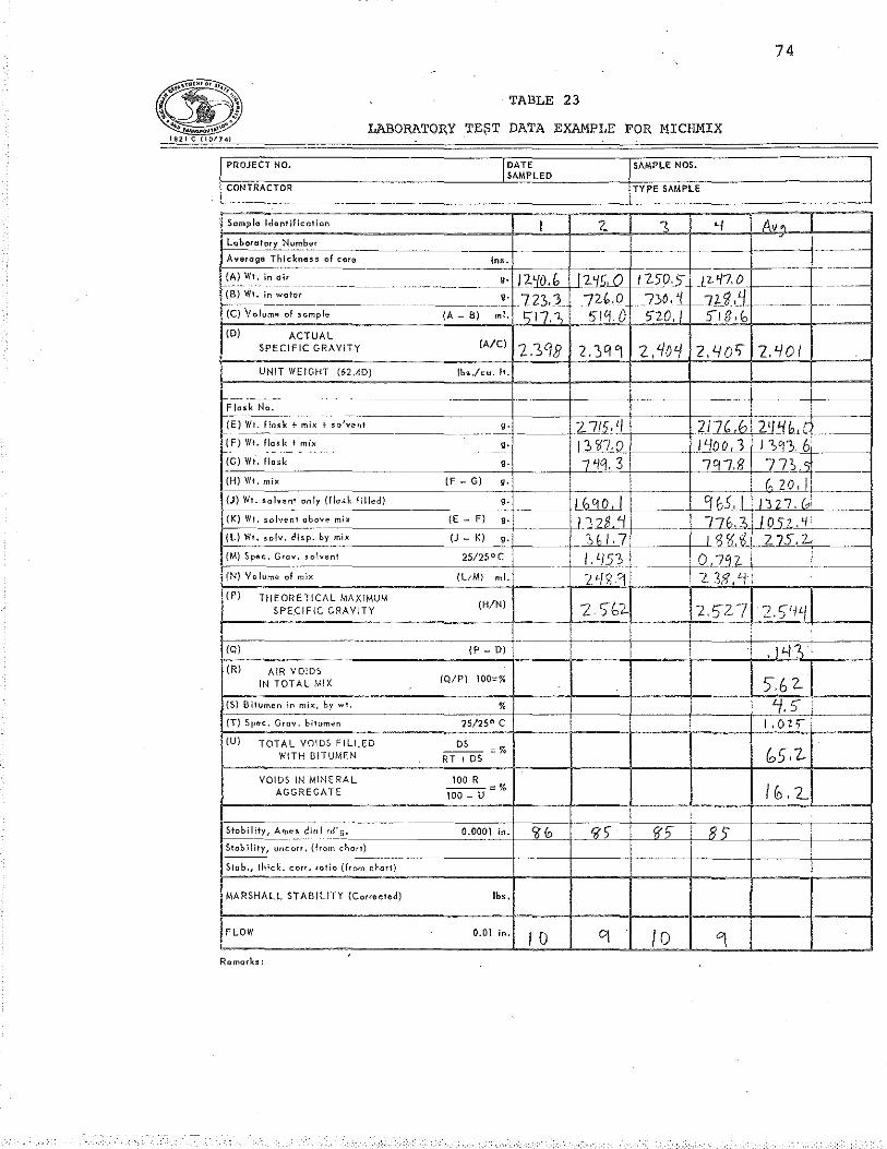
74
TABLE 23
'~·~·' . 1621 c !10174)
LABORATORY TE~T PATA EXAMPLE FOR MICHMIX
PROJECT NO. !DATE SAMPLE NOS. SAMPLED
CONTRACTOR TYPE SAMPLE
Sample ldontificotion I '2.. s '1 Avo ~~oratory Num~er
Averago Thickness of c(lre Ins. -~ '--~~- ·- --------- - --
{A) Wt. in air •· r11'1Q_.~ .1'1£.I2 cJ"2:50,..)_ p.q7. 0 ~--1-- ~--··--·-- - --- ------------~--- --------------- -----
(B) Wt. in water •· 723.} 72-lc.O 7:>0' 'i t--vs.~ 1-- -~ .. --~---------------- - ----------- -------(C) Volume of sample (A- B) mi. 1)17,' '510.0 -'i'lo.l ')18 •b (D) ACTUAL
SPECIFIC GRAVITY (A/C) 7_,<,qg 2.YI'l 2,'10'/ 2.40'> 7.'101 UNIT WEIGHT (62.40) !bs./eu. ft.
------ - .. ------------- ·--~- ----- ·-·· - -- t- -~ t----Flask No. f-'-::-: --- . -- z 715_,'j }l]C,A-2 ,_l'J~f,,( -· (E) Wt. flask+ mix +solvent •· ----- ---~ ·-~~----------· ---- ---- -----
(F) Wt, flask t mix •· i3'il7.o ... 1400,3 1'2,93 6 --~ . - -- --
(G) Wt, flask 9· 7~q. 3 79 7.il n~.' (H) Wt, mix IF - G) •· _£_2illf---~ {J) Wt. solvent only (flask filled) •· L6CJo.J c-'lfJ_._l /1 27. & ------- -- ------ ------(K) Wt. solvent above mix (E - F) ,. ___ U~f-'J 776:-~- .l05J..c'4--~--!-'-'--- ~--- . -(l) Wt. solv. disp. by mix (J- K) 9. I 3 1.7 ,-q)i 275.2 {M) Sp0c;, Grov. solvent 25/250( I I. '!53 0,7_'!2- ' f'-'-~-- ·i10i9 - ' (N) Volume of mix (l;M) mi. 2 3??,'-1 I (P) THEORETICAL MAXIMUM
(H/N) SPECIFIC GRAVITY 2 ')(,'2. ?.527 7.')'1~
I - ---- ~
(Q) (P- D) I ' I!../ 1, IRI AIR VOIDS
100:::% IN TOTAL MIX (Q/P) 5.62-(S) Bitumen in mix, by wt. % '-/.5"
-~
{T) Spec. Grov. bitumen 25/250 c I 1 .ozs- · lUI TOTAL VOIDS FILLED DS :::% k,5.2 WITH BITUMEN RT + DS
VOIDS IN MINERAL 100 R
I iD. 7_ AGGREGATE ---:::% 100- u
----· ----- ---- ----~, qj R) Stability, Ames dial rd'g. 0.0001 in. 'i)(o
-----·
Stability, uncorr, (from chon) -- ----------- --·----Stab., thick. corr. ratio (from chart)
MARSHALL STABILITY (Correeted) lbs,
FLOW 0.01 in. I 0 D\ /0 "'\ Remarks:
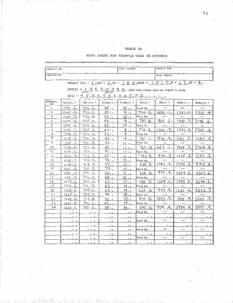
75
TABLE 24
WORK SHEET FOR EXAMPLE USED IN MICHMIX
I'R\lJECT "· 'OAH HSTE!'l SAI!1Pl E II o s,
CDIITRACHIR TYH SAMPU
&PHALT ITC ~]_,LEV~ .Q_,PS ~ _j_.l?._.J!._,SGAS ~ _I_._Q3o_.> ,N =~.±...,NT~ ..1_,
SGS(l) = _l._i 2._ _l_,_Q_, _ _]_ .9._ .1:._, (Fill boi:h blocks when one !iq~id h u"ed) (lr 1) (Ita t ~)
-- ------- -X(l) ~ ~ . 5' ,_s:. 0 , <;", 5, G. 0, (,. 5' .~ • .Q_, _ --MARSHHL WA I R( I) "' 'IIIlA T ( 1 ) " STAB(!)"' FLOW(!)= 'IfF (I} " \!IS ( 1 ) "' WFM( 1) "' WFMS(l)" ,w.
I 12~0 -G. 723 .. ~, ~6.' to., Flask No, -- -- --2. /1.~5" .o, 7L6 .c. ?5".' q ., 7Y'l ·3 • 1&90 ·I' 1337 ·0· 271> .'{, 3 11.5 0 . c;, 7'0 ·~· q 5" • ' 10·· !ask No, -- -- --4 IL'-n ·0· 72P . ~ ~ ~,.' Cj ., 797-l?, %5" .I' I ~00 .>, "217, .(, c; 12Y5 .2 72'1 .o )( (, . (0. hsk No. -- -- --G !LY~ .I' 724 .]. Si3.' B.' 726 .'/, 17L'1 .7, I-, 11 .z, 27/ti .(}.
7 12'10 .o, 77-2.... o, 8.,.' 9 . ' !Fta•k No. -- -- --2 /B9 .!,, 71; -7. ><O·' 9 . ' 7~1 -I' q77. .q, I'JII .c;, 2.1 "'~ .-z. g 1241' . I. 7>' .~. ~3.' II ·, I ask No. -- -- --
10 I ZY?,.: b, 7)S. 6, iS'5 . , J I . ' 7V'i · (), lf:h'> ·I, 14111 .3, 2.7()4.2., II \?_ 1,~ . ! , -n,\ .\, C!\ ., II., !ask No. -- -- --11 ]2_~7 .t, 7U .7, ~5., II . , ~~~7.9, '17~ .7, I :>OS .3 21'5'/ .3 l'l 12 ,g . ''• 72'1 .7, -,4.' "' . ' !Fla!k :-io. -- -- -/Y ~.I-, 7/g. 7 77. "· <;,sq . s 11q I .4 17.'10 .3 271'2. .8. ,, 1n1- . b, 711 .), 77., I 12. . ' lask No. -- -- --I' 12'1S . 1', 71'1 .'\ {;,() . , II. t,zs .o q77 ,q 122.'1 .z., 2.013 .£_, L7 1"1...~0 . 3, 71 ~ .z. (,9. lb . Fla 1k No. -- -- --1£ )"'2.1~/.(,, 7ln .o, ?.1. ' I <;. , 741\ .5, lb';\J .~. l'l1~ .8, H4q .:>,
f---1.1..___ I '2 '.Q....2..,_ 714 .3, ~ '\., IY . lask No. -- -- --20 1230 .g, 720.2, 6']., I <J • , !,<; .'1., "117 .q, !HI .b, '2.01,(, .7, ?I IU<;.(,, 712 .. 3 59. I >I • Fls3k No. -- -- --1'2 )1.1£"·2. 7138, '>< . ' /.0.' g7R .~.
'""' .7, 15'10 • "[, 7(;~7 .-1
2} 12L3 ·-'· 7/ z... I , G 1. . 17. · Flask No. -- -- --1'1 \].~I · I, 7f7l .I, ss . , 7() • ' ~41' .o. 97~ . 'I, I"Zl9 .~ • '2017 . '-/,
' ' . ' ., !ask No. -- -- --. . ... . ' .
' ' ., ., Flask No, -- - --
' ' .. .. ' ' ' . • ' ' . ' . ' Flnsk No, -- -- --' • ., . ' ' • ' • • ' . ' ., Flask No. -- -- --' ' . , ., ' • • •
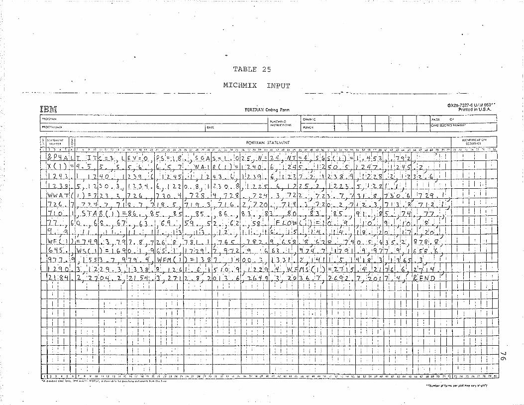
. I
TABLE 2.5
MICHMIX INPUT
FORTRAN Coding Form
. -- ... .. - -----·-----
GX2B-7327·6 UIM oso•· Printed in U.S.A.
; I ' i ' I I . I : ' ' ' I ' ! i i I I i I I I I I I I I I 'It: 1 : I,,,,' 1: 1 1 ir 11:, 1 i! 1111 11111: 1llll!l
I i ' I ' : I ' ! I : I . I : : :·I : I I I : I : I I ! I i I i I I I I i I I I ! i i i ~tt I I ·II I i II j : i! I ::I I i: i ! : i] ::! i 1111 i! II I iII iII iiI i 111_1 I
1: :!: ,; ii ! i!i' rj :,il I i i,•! I iii :ill !Ill" illi ,1:1!! i iJii __ u i I : I- i I l i ! I: i I i I i I ! I i i ! ; i ! 1___l i i : : ! i ! I i l_l iJI i : I ! i IJI I ! I ! I ' i i I I "i : i I : I : I : i i I I I I I I ' ! I I i I i i I I -...,J
I I- ! : ; I : ! I : ! : - : I : I I ! I i : ' i I ! I : ; I ! ij "" , : I I I : · i . : : I I I [ I I
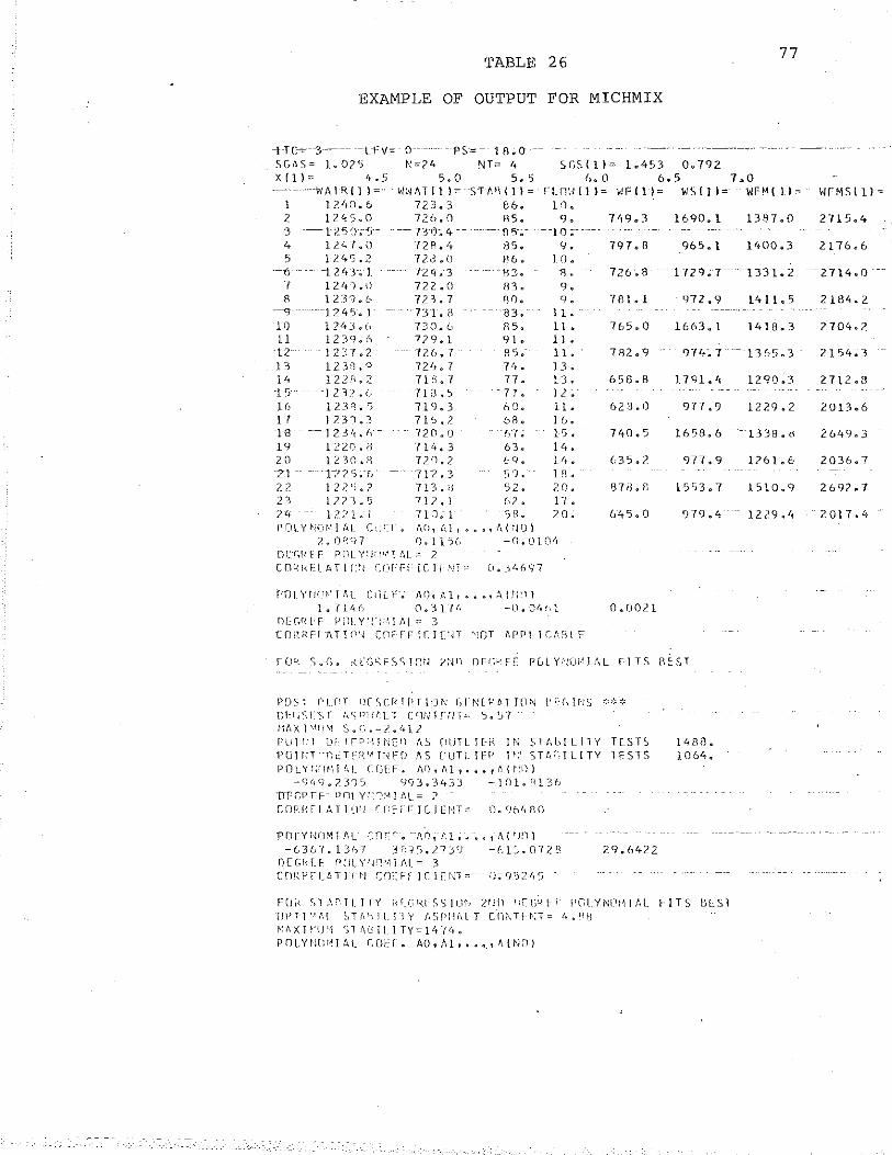
TABLE 26 77
EXAMPLE OF OUTPUT FOR MICHMIX
-nc~--3---- -t-Fv~o----- -ps~-rs;(} --SGAS= l-025 ~=24 NT;;;: It SGS(ll= 1~453 0$792 X{l)= '•-5 5.0 5. 5
s-TI'I 1HU= 86.
6.0 6o5 leO --WA!Rl1 )o H:<ATI1 }o
1 2
lZ't0.6 1245.0
-3 -~r2o'.1•5-1247.o
723.3 72.6.0
----r:ro-.. 4
rtn:-1111~ WF11l" WS(ll" WFM(ll" 10.
4 5
---(}'
7 R
..------q·---
10 ll 12 13 14
16 11 -Is 19 20 ·z!u 2'1 2_4-
124'5.2 -!243;1 12ft I .. \) 123'L6
--1245.! 124J.(• 1239~6
-1237.2 123'1. 0
12211.2
123l. s 1 ?.3'L3
---J231t,h'--
1220.0 12 3l"Li--l 1-z2s.-r)· 1 2 2 ').? 12? '). fj 12?1.1
72R.4 72.i.LO 724.3 722.0 72'. 7
· 731. B 730~ (_, 729.} 7?_6.7 72 1t. 7 7 Ul. -, 7!3.S 719.3 716.2 720.0 714. 3 1zn.z 712.3 7D.I_l
RS. 9. -----115-~-- ---to;
85. 9. 86. !0.
83~
RO. '83. -
R5. 91. 8 s .-7 1t • 77.
-n. 60. 63. '67 .. 63. [:4. S').
52.
"· 9. 9.
1!. !I. 1 ) • 11. 13. 13. 1 2. ll. 1 (). 15. 14.
71? 0 1 (,2.
l 1f •
1'1. 20. n. /:0. 710.1 ')8.
1\(J, {.,1, ••• ,t\(~JfJ) 1.0 1~CJ7 f).ll'JC -0.010 1~
11~-r'".;Kf: F PnL Y!YI','1 .1\L::: ;:?
CGRI<ElATif 1 ~.) (OFF!- ICir-.~!1= 0.34697
PO\ Yi!\_Wjt,t_ CCI[ f-. Af) 1 /,1 1 ••• ,!:<(!'i'lJ l.7lfd, 0.31"(1, -O.QI,!,
D/:Gf<l·f !Jfl!.Y~·!'i:-',J AL-:o: 3 LrH~Rft-,t;.T1f1'~ COFrFI(l['H ''!OT 1\PPLJ(.,',:'\ F
~;A X j \\i I\\ S J, . ::::? • ltl ?
749.3
797.8
7 8]. 1
782.9
658.8
623.0
(,35.2
87B.8
0. 0021
PUJLT 8i· rr~;J:.\JN[11 f'IS \1UTL TFk JN 5'-Tt,bl LTTY TrST.S l'OJr;r--n~r::RMTr~FD f\S l_lUTL IFf! rr:• STf,I,TLlTY TESTS POLYI;rH·\1 t.j_ COfF. J\1), /11, •• 01 1\. U-111)
-~~9.?31S 993,343] -lOl~Rl36
m~r,p rr- VrJJ Yi:J!.lJ L\t_ = 2 COP!~ II ,'.,Tl•.JI! r.f:f:f FICltf'lT:::: 0,f)t;:.tifl0
-rnrvr~or.nr-L- r_n~:~·.--An,t.t, .... ,A..('H1l -63b7.13G7 3R15.27J9 -~1~.0728 29.fA22
OEGkll rrJLYNn~lAL= 3 CrJJ-.;l'fU<TlmJ CrF-Fr lClEH1=--- rr;rJ')2l,:J
1690.1
965.1
972.9
977.9
977.9
fJ79.4
FUH. C.L\:-o-TLllY r~f_(;RrSSIIJ~ .. 21JO nt:G'-'!:-1" f'[,l_YNL'~I~lf·L FlTS t>EST OPTT'-',<.1 STt,(-:,fLJ'fY f1SPil/1lT CCi~Tf~·;T:o lt.f~tl
f.1AXJ!·'U'1 ~;1 :\l<ILI TY-::::ltt.f<t. POLYtJn:~IAL COtr~ AO,;\lt·~~-~A{N:-1)
1387.0
lft00.3
141!.5
1418. 3
1229.2
1?61.6
1510.9
1229.4
HrMS! ll =
2715.4
2176.6
2184.2
2704.2
2712.8
2013.6
2036.7
2 692.7
'2017.4
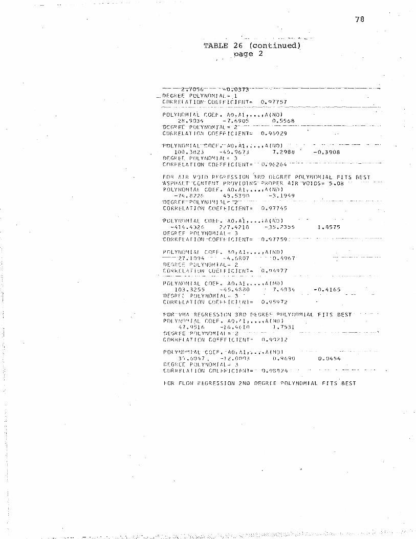
78
- ..__ "' -
TABLE 26 (continued) page 2 ·
-- -·z-c7o'56·· · ·- ·- ··1l ;1l37T--·-·· ---····----·-·---------·--·
_DEGREE POLYNnM!hl.= l CORRFLAfiON COEFFICIFNT= O.Q7757
POLYNOMT~l (OEF. AO,Al,.~.;A{NOJ ~B.9034 -7~0905 0.5568
"t)ff,P EE- --pOLY NOM r 1\L =·--"2·-· --- -------CORRFLATJnN CnEFFICIF~/1= 0.9S929
"Pnt.Y NrHn At· r: ntF .-- llO, A1, •• ~ ,-n.-um) 100.3BZ3 -4~.9673 792988 -0.3908
fJ[GI-'EI?. POLY~JO~li/lt-= 3 -c-nHFF.L-ATION COfFFICIUH= 0.9(,264 --
FOR AIR V~JD REGP[SSION 3RD O~GREE POLYNCIMIAL FITS REST ·A-s-PHtd:r-·-cuNTFNT PlHJVIOlHG- P;<,nPF~ ATR -VOl OS== ·s,.OH POLYNOMIAL CDEF. AO,A!, ••• ,~{~InJ
-74~R22A 4~.539n -3.1949 ·DE GP r F ---p fll Y I'Fl11J _·i l = L. CORRELATION COEFFICIENT• 0.97745
-Pot.Y:~'li·H-tll- C1lF.F.· ·1\.o,-A·l, .... !4-{NOl -41~-4326 ?27.4210 -35.?355
DEGREF POLYNOMIAL= 3 roKR r·t 1\ f I CJ~J --CoFn·- f (. H-NT::: - Q .--<'J"l7 59.
POLYt-lf!Ltit..L COEF. r'I.O,Alt•••tAINO) ~----27. 10'14 -th(,{W7 0. 1t907
DEGREE P(JLYNOMIAL= 2 CO~kfl.AflUN LIJE~FICI[NT= o.q~q77
POLYNilf.\Il\L COEF$ /i0~t\1 1 ~ •• ~t,(HOJ 103.3255 -45.4nao 7.6134 -0.4!65
i)f-'(',f/U PtJL YNOf'ti /IL=- 3 CUKREL/1T!l1N COFFf--ICirNT== Oo'-J5972
r:-m~-v~1/\ REG!.{fSSlON -3Rf) N:GRE-f PflLYI-~Ilf·11AL FITS BEST PflLYNn'~IAL. C!lEF. A0,~l, ••• tA!NI1)
47.Y~l6 -1&.4610 1.7~31 nttiRFE -POLYN~MIAL~ 2 COkl<.fi.ATlON COF:F-TIClf:NT= 0.99212
i'Ol-v~.J[_l'lh'IL (.CJ[P. ll,Q-,At;·· ... -.;,/l(l')l_l}
30.60~7. -}2.0003 0.,9690 0.0454 D~GPEE POLY~OMJAL== 3 t:tJRHfUl.TION CflEf-"f·JCIF-:H= -o.,<JflfJ?'f
FOR FLOW REGRESSION 2ND DEGREE POLYNOMIAL FITS BEST
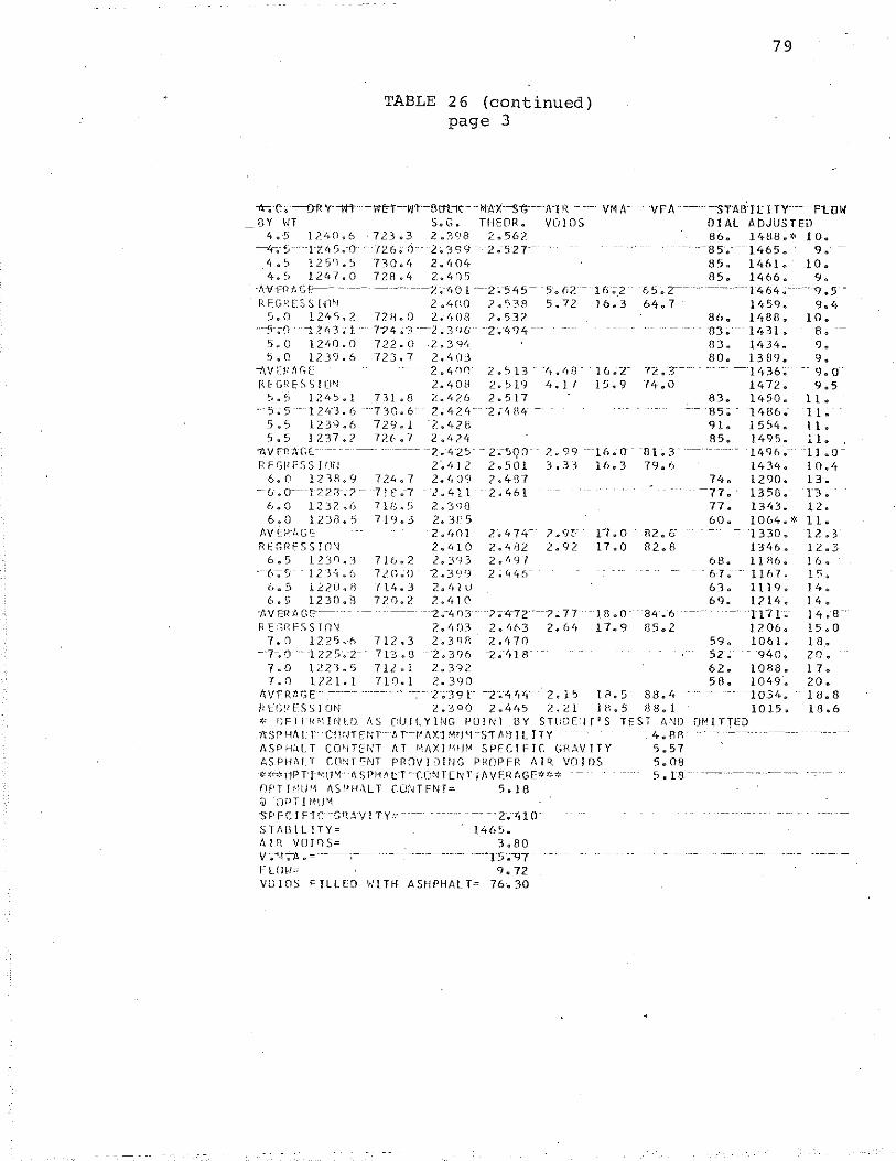
TABLE 26 (continued) page 3
79
"k;;f-;·----t:rf<Y-vt'f·--I<E-T--wr·-Btft><c- ·MAJ<--,-r;-- A-IR ·-- ·· VM A· -- VFA ----·--sTAB.I U Tv·-- -FLOW BY fiT S.G. THEOR. VOIDS DIAL ADJUSTED 4~5 1Z40o6 723o3 2.398 2~562 86o 1488.* lOo
-q:-.--:;-· -u~~~~)~-o 726~-0- 2o399 2.-527-- --ss·.---1465.. 9 .. --4.'> 125'l~~) 730.'t 2.1t04 85~ 1461 .. 10 .. 4.s 1247.0 7ZB.4 2.4n5 as .. 1466. 9.,
-11-v;~-n n. ·ct;.,_____,_ __ ----- ·------··-----:.:.-,to 1 ---2;. 54 5- -s· .. (j?.- - 16·;-_2 -- 6 5 .. z-- -- - 1 4 64 ~----- -- 9 .. 5 -RF.GkFSS lfl~l
5.0 12't5~~ 2.400 2.538 5.72 16.3 64.7
?. 532 72H.O 2.t,OB 7-'?4 .3-----2.346' 722.0 -2.3<;14 723.7 2.403
-5-.---0 -1.?'1-3.-j S~O 1240.0 5~0 1239.6
7\Vi:F Ma_:-- -- ---z .4nrr 1{!:-"GRE-SSJU~J 2.110H
5.5 12'+5 .. 1 rn .a 2.4?.6 s-.-s-"" 121-d.6- -730.6 2.'424-5~5 1239.6 729.1 "2.428 5.5 1237.? 72~.7 2.424
2. 494---
-2.5 13 2.519 2.517
16 & T 72.3-----15.9 74.0
·t.v r-r.:-;\-(;£_------ ··- -~- -------- --z. 4 '2? · -- z-~-sQ o·- z. 99 -- 16 .. o - -ot. 3 ·
RFG!<ESSIOI~ z··'•l2 2.501 3.33 16.3 79.,6 6.0 l23R.9 724.7 2.409 ?.4B7
--6 • o--- 1"2 21L 7 -- -71 g .-7 - 2. 4 1 1 - 2 ~ 4 61 6.0 1232.6 718.5 2.3q8 6.0 1238~5 719~3 2~3P5
1\V-fP-A"G-t_::- -----· -"---------- --· z-;;-1~01 ---7.-,-4 74·-·- ?-;,----qf-
RF.Gf<FSSI0'4 2~410 2.482 2~92 6~5 123f)~J 2of•97 7lfh 2 2.393
---()----;:.- "12'3·t.b 2.446-7 20.0 --z ~3tJ9 fl4~3 2. It] U
7 ?.0~2 ?_ 0 It ]_ ('
n.o 17.0
& .. 5 1L204B 6.~ 1230.8
·AVfi~AGr:--- .. --- --R E:-;RESS IO'l 7~0 12Z5.·f>
-2.403. 2. 403
2;4-72 ---;>.77 ·1s.o· 2.463 2.64 17q9
_ .. 7-~ o --- -1z2s·.-z--7.0 1221.5 7.0 1221.1
712.3 713 ~ 8 712. I no.1
2.38R --z. 396 2. 392 2.390
8£(,;6 ---1]5 .. 2
1459. 86.. 1488 .. 83. -- l't31 ..
83.. l'd'tG 80. 1389. ---.-1436.
83. 85 •. 91. 85.
74. -n ..
1472. 1450. l't86 .. 1 5 54. 1495. 1496. 1434. 1290. 1350. 1343. 77.
60. 1064.* .- 1330 •.
1346. 68. 1186. 67. JIA7, 63. 1119. 69. 1214.
Tl7l' 1206.
59. 1061. 52; 940., 62. 1088. 50. 1049.
·1\V'FRAt;E-·----------- --2~Atr4-·2.15 1P..5 88.4 -1034 .. -;?-~-391-
REGL'fSSION 2.,300 2 .. 4't5 ?..21 111.5 H8.1 1015. * GFTf"f{~\HlfU AS OUTLYING PUINT BY STUOE:n'S TEST .1\ND OMITTED 7\:SP HI\ L r- -c-n~H fNl - f:, ~--f-1!\X-J MtJ'-1 --s-,- /1111 L f TY 4., RA · ASPH~LT C0'1TfNT AT MAXli~!J~ SPECIFIC GRAVITY 5.57 ASPH1\I T CO~H'::i'JT PI~OVIDII-lG PROPFR AIR, VOIDS 5 .. 08
·* :<n~rJP r·p.~ t1V. '!\ S PH-" t-T --coN T [NT ; A Vf.R t,G[*':--* -- 5 ~ 13-0PTJ~lJ'1 AS!>H~LT CONTENT= 5~18 @ -i.JPT I ,'},\1'1 "SP Fc-f FH: --cn.,tV 1 TY~ -- 2&--lil o· ST/\l)lllTY= 1.465., AIR VOF1$= 3q80 v-;•-t-;-A -. = ·--- ;--- ---- ·-- --------- - · r5 '""7 · FUli-J:o 9 .. 72 VOIDS FILLED WITH ASHPHALT= 76•30
9.4 10.
B • --9. 9.
- 9.0 9.5
11. ll. II. ll" li.o-1 0.4 13. n.-12. 1!. 12.3 12 .. 3 1 6 .. 15 >
14. 1 4. 14.8. 15.0 18. 20. 1 7. zo. 18.8 18.6
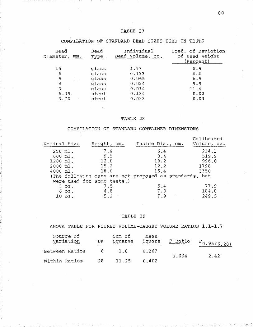
80
TABLE 27
COMPILATION OF STANDARD BEAD SIZES USED IN TESTS
Bead Bead Individual Coef. of Deviation Diameter, mm. ~ Bead Volume, cc. of Bead Weight
(Percent)
15 glass l. 77 6.5 6 glass 0.133 4.4 5 glass 0.065 6.5 4 glass 0.034 9.9 3 glass 0.014 11.4 6.35 steel 0.134 0.02 3.70 steel 0.033 0.03
TABLE 28
COMPILATION OF STANDARD CONTAINER DIMENSIONS
Calibrated Nominal Size Height, em. Inside Dia., em. VoluiUe, cc.
250 ml. 7.6 6.4 234.1 600 ml. 9.5 8.4 519.9
1200 ml. 12.0 10.2 996.0 2000 ml. 15.2 12.2 1798 4000 ml. 18.0 15.4 3350 (The following cans are not proposed as standards, but were used for some tests:)
3 oz. 3.5 5.4 77.9 6 oz. 4.8 7.0 184.8
10 oz. 5.2 7.9 249.5
TABLE 29
ANOVA TABLE FOR POURED VOLUME-CAUGHT VOLUME RATIOS 1.1-1.7
Source of Sum of Mean Variation DF Squares Square F Ratio F0.95(6,28)
Between Ratios 6 1.6 0.267 0.664 2.42
Within Ratios 28 ll. 25 0.402
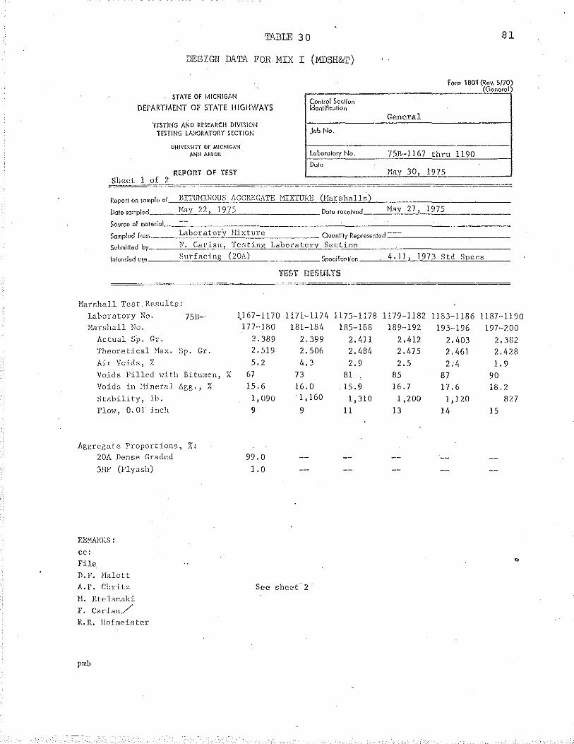
TABLE 30
DESIGN DATA FOR MIX I (MDSH&T)
STATE OF MIC!I!GAN
DEPARTMENT OF STATE HIGHWAYS
TrSTING AND RES[ARCH DIVISIOfi TESTit~G LMORATORY SECTION
S_hect 1 of _2
UHIVCRSITY OF MICHIGAN ANH ArWOit
R<PORT OF TEST
Con!rol Scc.Ho~ Identification
Job No.
l.oboralory No.
Dolo
81
Form 1801 (Rev. S/70) (G I) )Onora
General
75B-1167 thru 1190
May 30 1975
Roport on wmplo o! BITU11INOUS AGGREGATE HIXTURE _Qfarshalls"'--------------
Date smnpled --"J1~a_,_'_:c22oc.,__1"9ec7ec)o__ ________ Doro rocoived __ __clcc1a~y'.c--'2cc7~,'.c--'1C:9-'7"'5-
Source of material ___ -=:_ __ --:--:--:-- ---------'------------- -----Samplod from Laborator"y_ .. H:ixture Ouonlily Reprosonted_-_-_-__________ _
Svbml!ted by F. Caria_!l_t_Testing Laboratory Sectio,,n ___ _
lnlondod us.o Surf acing CW!i) Spocilkotion 4. 11! 1973 S td Specs
11arshall Test. Results:
Laboratory No. 75B-Narshall Nt).
Actual Sp. Gr. Theoretical Hax. Sp. Gr. A-:._r Voids, %
Voids Filled uith Bitumen, Voids in Hineral Agg..,
Stability, ]_b.
Flmv, 0. 01- inch
AggrPgate Proportions, %· 20A Denc,e Graded
3HF (Flyash)
REHAJU(S:
cc: File
D.F. Halott A.r. Chritz H. EtL'lamaki
F. Carlan./ R.R. Hofmeister
pmb
% %
1.)67-1170 177-180
2,389 2.519 5.2
67 15.6
1,090 9
99.0 1.0
1171-1174 181-184
2.399 2.506 4.3
73 16.0 . 1' 160
9
See sheet-· 2 ·
1175-1178 1179-1182 1183-1186 1187-1190 185-188 189-·192 193-196 197-200
2.411 2,412 2.403 2.382 2.484 2.475 2. 461 2. 428 2.9 2.5 2.4 1.9
81 85 87 90 15.9 !6.7 17.6 18.2 1,310 1,200 1,120 827
ll 13 11, 15
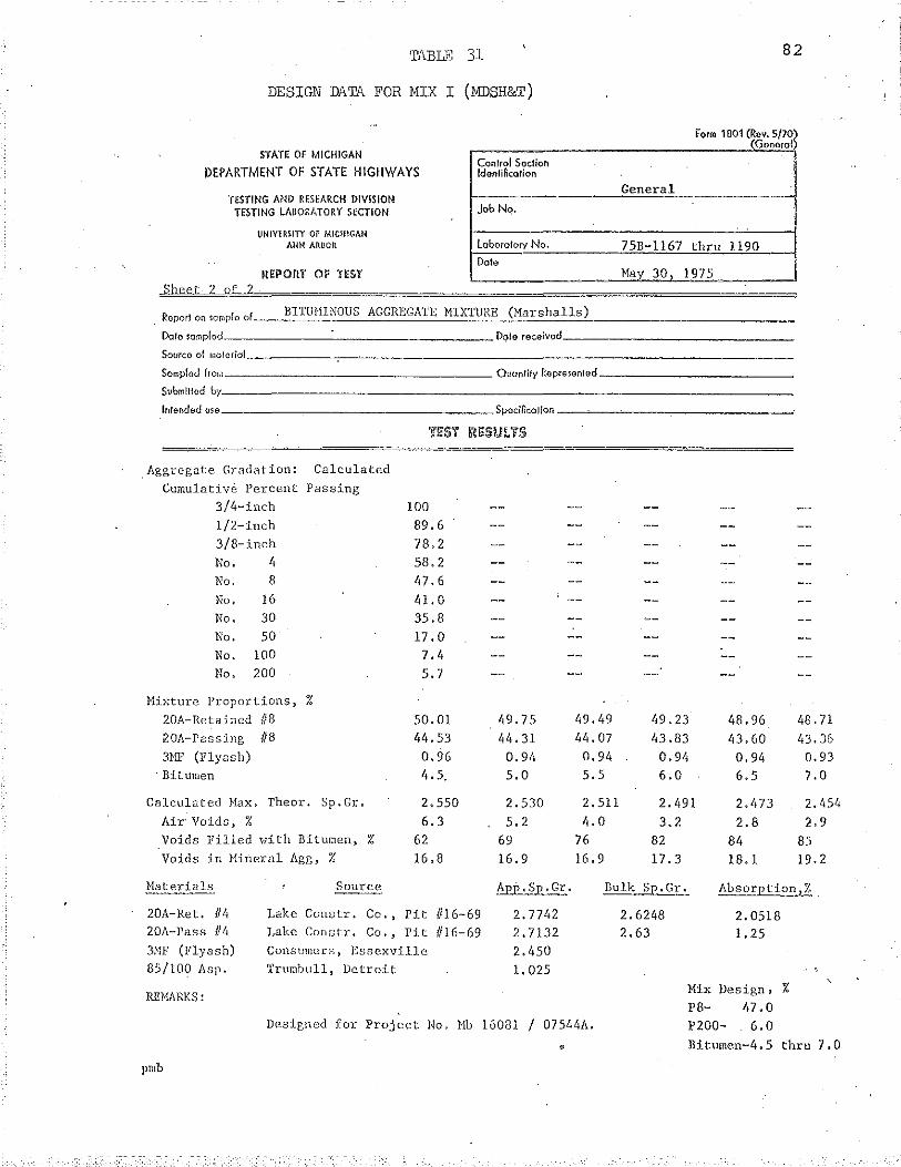
TABLE 31 82
DESIGN DATA FOR MIX I (MDSH&T)
STATE OF MICHIGAN
DEPARTMENT OF STATE HIGHWAYS
TESTING AND RESEARCH DIVISION TESTING LABORATORY SECTION
Sheet 2 gf 2
\JHIVERSITY OF MICHIGAN AHH ARDOR
REPORT OF TEST
Control Sodion ldonti~colion
job No.
laboratory No.
Dole
General
75B-1167
May 30
Form 1£101 (Rev. S/70) (G e I) on ra
thru 1190
1975
BITUHINOUS AGGREGATE MIXTURE (Marshalls) . Roporl on $Omplo of--=========_::__=="="'-~"-"'==='--------------Daro samplod _________________ Dqlo received ______________ _
Source of woloriai _____ ~----------------------------
Sampled from----------------- Ouonlify Represon!ed ______ ~----~
Submltlod bY------------------------------------
Intended use _________________ Spodllcotion __ ~----~-------
Aggregate Gradation: Calculated Cumulative Percent Passing
3/4-inch 100 1/2-inch 89.6 3/8-inch 78.2 No, 4 58.2 No. 8 47.6 No, 16 4!. 0 No. 30 35.8 No. 50 17.0 No. 100 7.4 No. 200 5.7
Mixture Proportions, %
20A-Retained 118 50.01 49.7 5 '•9. 49 49.23 48.96 i20A-Passing /18 44.53 44.31 44.07 43.83 43.60 3HF (Flyash) 0.96 0.94 0.94 0.94 0.94
·Bitumen 4. 5. 5.0 5.5 6.0 6.5
Calculctted Hax. The or. Sp.Gr. 2.550 2.530 2. 511 2.491 2.1•73 Air Voids, % 6.3 5.2 4.0 3.2 2.8 Voids Filled Hith Bitumen, % 62 69 76 82 84 Voids in Hineral Agg, % 16.8 16.9 16.9 17.3 18.1
48.71 43.36 0.93 7. 0
2.454 2.9
85 19.2
Haterials Source App.Sp.Gr. Bulk Sp.Gr. Absorption,%
20A-Ret. 114 20A-Pass 114 311F (Flyash)
85/100 Asp.
REHAHKS:
pmb
Lake Con.str. Co., Pit IJ16-69 Lake Conr~tr. Co., Pit //16-69 Consumers, Essexville Trumbull, Detroit
2. 7742 2. 7132 2.450 l. 025
Designed for Project No. Mb 16081 j 07544A.
•
2.6248 2.63
2.0518 l. 25
Hix Design, % P8- 1,7,0
P200- 6.0 Bitumen-4.5 thru 7.0
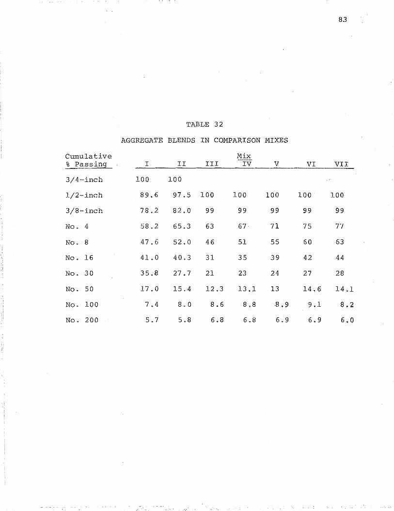
83
TABLE 32
AGGREGATE BLENDS IN COMPARISON MIXES
Cumulative Mix % Passing I II III IV v VI VII
3/4-inch 100 100
l/2-inch 89.6 97.5 100 100 100 100 100
3/8-inch 78.2 82.0 99 99 99 99 99
No. 4 58.2 65.3 63 67 7l 75 77
No. 8 47.6 52.0 46 51 55 60 63
No. 16 41.0 40.3 31 35 39 42 44
No. 30 35.8 27.7 21 23 24 27 28
No. 50 17.0 15.4 12.3 13.1 13 14.6 14.1
No. 100 7.4 8.0 8.6 8.8 8.9 9.1 8.2
No. 200 5.7 5.8 6.8 6.8 6.9 6.9 6.0
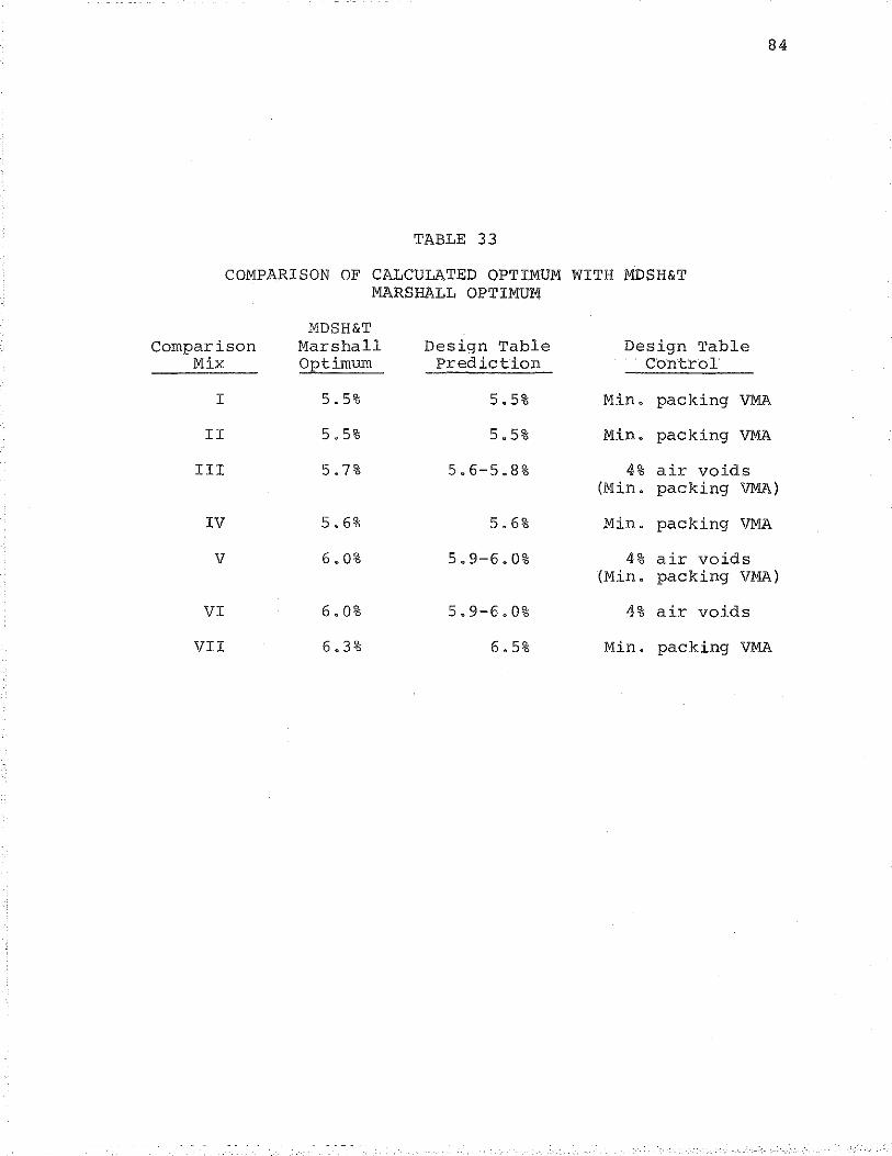
84
TABLE 33
COMPARISON OF CALCULATED OPTIMUM WITH MDSH&T MARSHALL OPTIMUM
MDSH&T Comparison Marshall Design Table Design Table
Mix Optimum Prediction Control
I 5.5% 5.5% Min. packing VMA
II 5.5% 5.5% Min. packing VMA
III 5.7% 5.6-5.8% 4% air voids (Min. packing VMA)
IV 5.6% 5 .. 6% Min. packing VMA
v 6 .. 0% 5.9-6.0% 4% air voids (Min. packing VMA)
VI 6.0% 5.9-6.0% 4% air voids
VII 6 .. 3% 6.5% Min. packing VMA

FIGURES
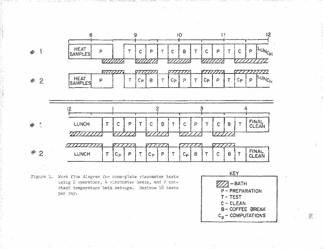
8 9 10 II 12
# 1 lsA~Et~s~ PWJJ r~jr u~ T ~l;J T [j~~H # 2 HEAT p T Cp B T T Cp p T Cp p LUNc
SAMPLE H
2 4
# 1 ;;:J T l±J T ~~l;J T lizJ;J T c:Jj T I FINAL I CLEAN
#2
Figure l. Work flow diagram for cone-plate viscometer tests ·using 2 operators, 4 viscometer heads, and 2 con
stant temperature bath set-ups. Maximum 18 tests per day.
KEY
I FINAL CLEAN
~-BATH P- PREPARATION T- TEST C- CLEAN B- COFFEE BREAK
C p- COMPUTATIONS
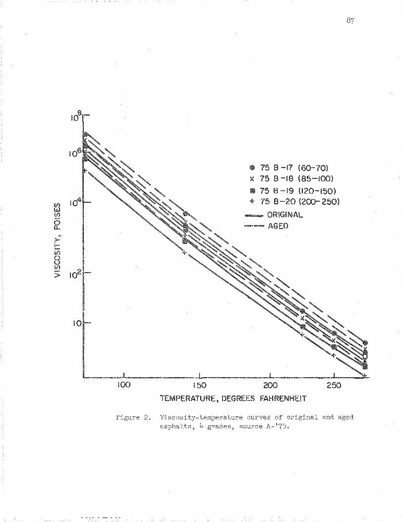
10
100
• 75 8 -17 (60-70) )( 75 8-18 (85-100)
1111 75 B -19 (120-150) + 75 B -20 (200- 250)
-ORIGINAL
150 200 250
TEMPERATURE, DEGREES FAHRENHEIT
Figure 2. Viscosity-temperature curves of original and aged asphalts, 4 grades, source A-'75.
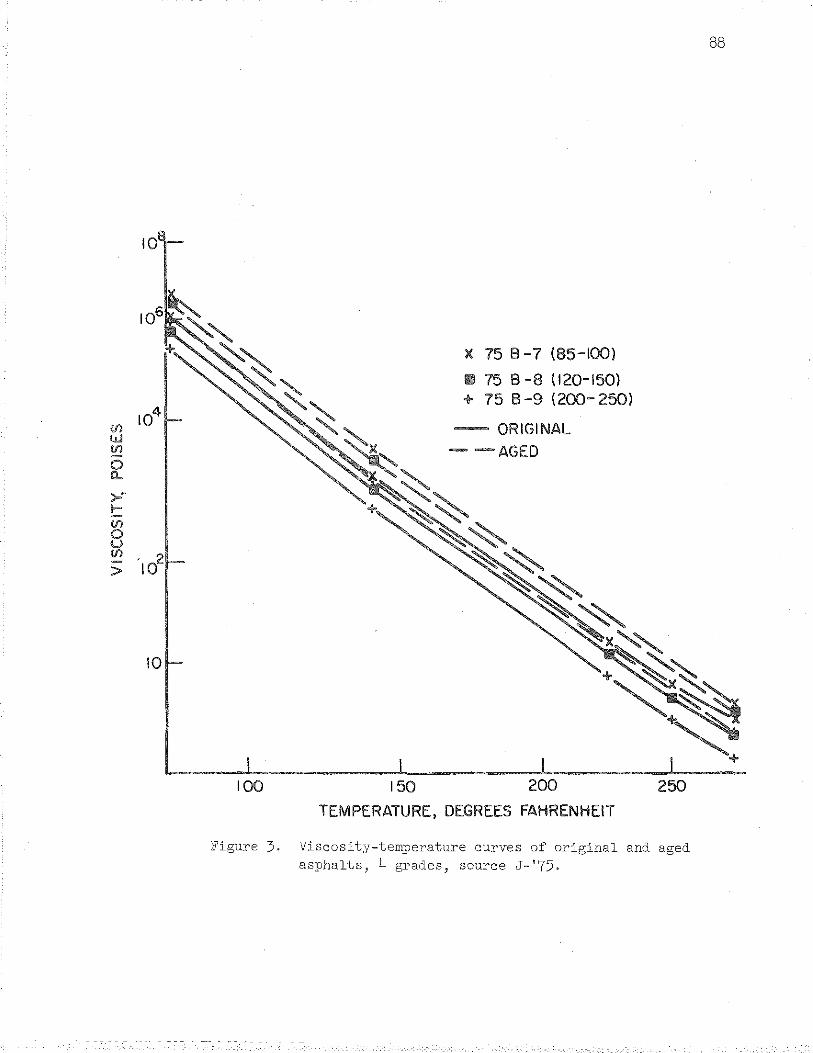
10
If) IJ.J If)
0 a.
>" 1-If)
0 u If)
'lo2 ->
10
100
)( 75 8 -7 (85-100)
Ill 75 8 -8 ( 120-150) + 75 8-9 (200-250)
-ORIGINAL
--AGED
150 200
TEMPERATURE, DEGREES FAHRENHEIT
250
Figure 3. Viscosity-temperature curves of original and aged asphalts, 4 grades, source J-'75.
88
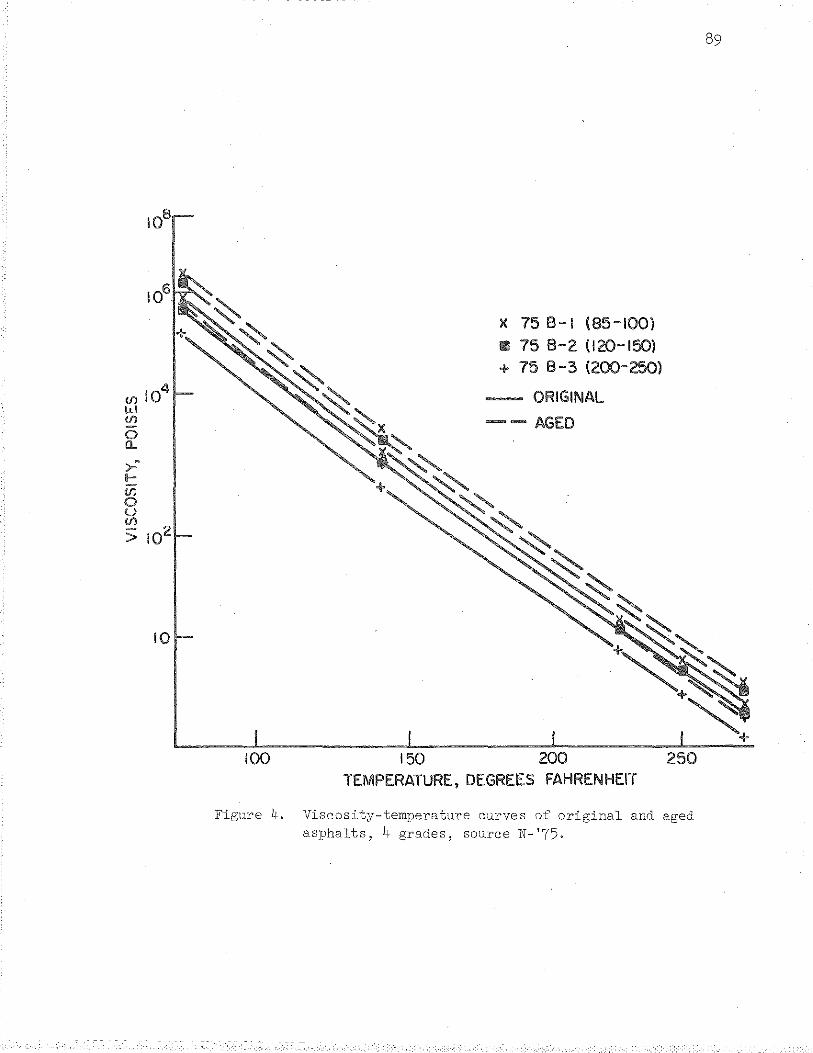
(f) I 04
w (f)
0 Cl..
;.: 1-(f) 0 u (fJ
> 102
10
X 75 B-1 (85-100) II 75 8-2 (120-150) + 75 B-3 (200-250)
-ORIGINAL
--AGED
100 150 200 TEMPERATURE, DEGREES FAHRENHEIT
Figure ~. Viscosity-temperature curves of original and aged asphalts, 4 grades, source N- '75.
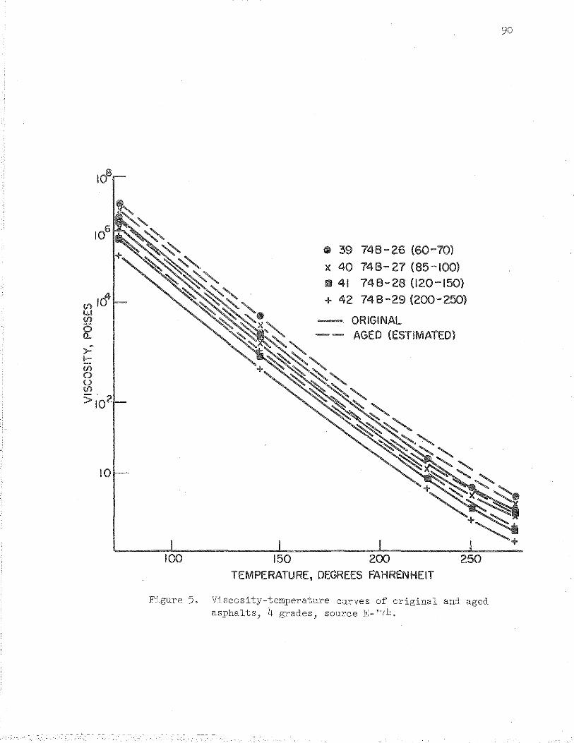
10
100 150
• 39 748-26 (60-70)
)( 40 748-27 (85-100) Iiiii 41 748-28 (120-150) + 42 74 8-29 (200-250)
ORIGINAL
200 250 TEMPERATURE, DEGREES FAHRENHEIT
Figure 5. Viscosity-temperature curves of original and aged asphalts, 4 grades, source E- '74.
90
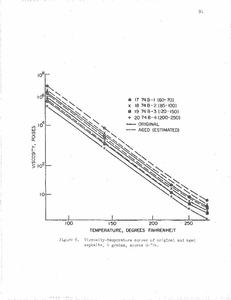
10
100 150
• 17 748-1 (60-70) )( 18 748-2 (85-100) II 19 748-3(120-150) + 20 74 8-4 (200-250)
-ORIGINAL -- AGED (ESTIMATED)
200
TEMPERATURE, DEGREES FAHRENHEIT
250
Figure 6. Viscosity-temperature curves of original and aged asphalts, ~·grades, source G-'74.
91
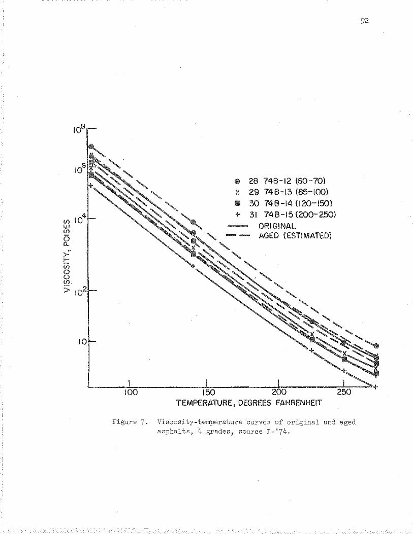
106
(!) w (!)
0 11. ~
>-1-(!) 0 u If).
> 102
• 28 748-12 (60-70) X 29 748-13 (85-100) Ill 30 748-14 (120-150)
+ 31 748-15 (200-250)
ORIGINAL -- AGED (ESTIMATED)
TEMPERATURE, DEGREES FAHRENHEIT
Figure 7. Viscosity-temperature curves of original and aged asphalts, 4 grades, source I-'74.
92
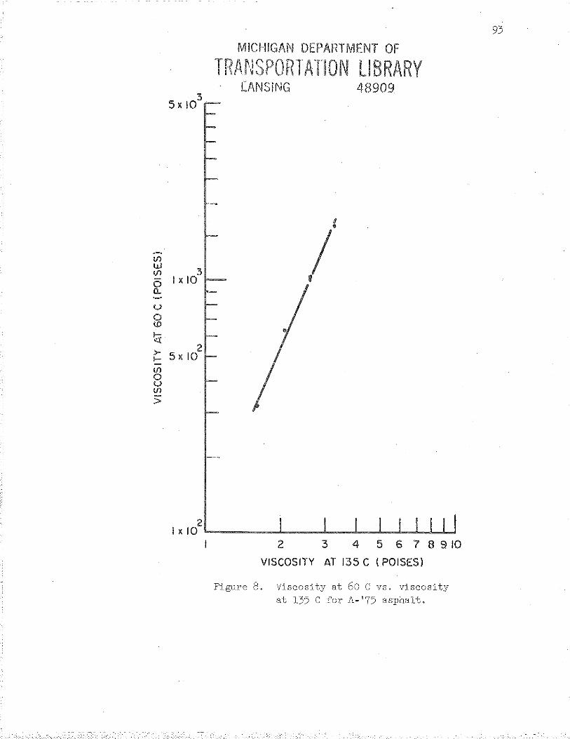
Vl
3 Sx 10
~ 3 0 I X 10 a..
u 0 \D
~ )-1-
Vl 0 u Vl
>
MICHIGAN DEPARTMENT OF
THANSPORTATION LIBRARY LANSING
/
2 3
8 •
48909
4 5 6 7 8 9 10
VISCOSITY AT 135 C (POISES)
Figure 8. Viscosity at 60 C vs. viscosity at 135 C for A-'75 asphalt.
93
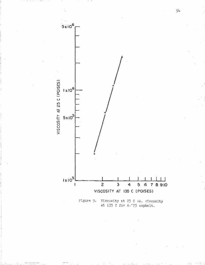
Vl w tf)
lxi06 0 a_
u I() N
~ )-1-Vl 0 u IJ)
>
•
•
VISCOSITY AT 135 C (POISES)
Figure 9. Viscosity at 25 C vs. viscosity at 135 C for A-'75 asphalt.
94
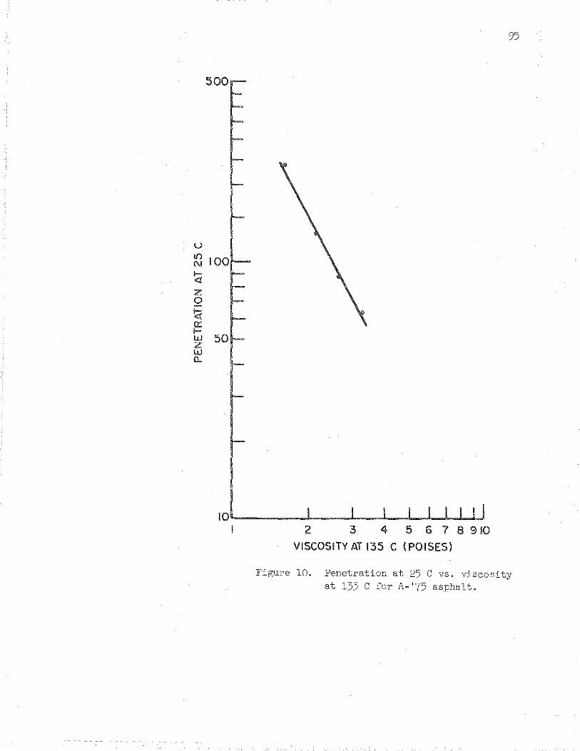
u I{) N
~ z 0
'<i a:: 1-w z w 0..
95
500
IOL-------~----L---b-~~~~~
I 2 4 5 6 7 8 910 VISCOSITY AT 135 C (POISES)
Figure 10. Penetration at 25 C vs. viscosity at 135 C for A-'75 asphalt.
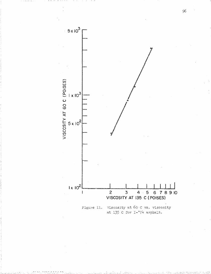
~
(f) w Vl 0 e:_ I x103
u 0 (b)
!<{ )-
:;; 5 )( 102
0 u (f)
>
Figure ll.
2 3 4 5678910 VISCOSITY AT 135 C (POISES)
Viscosity at 60 C vs. viscosity at 135 C for I-'74 asphalt.
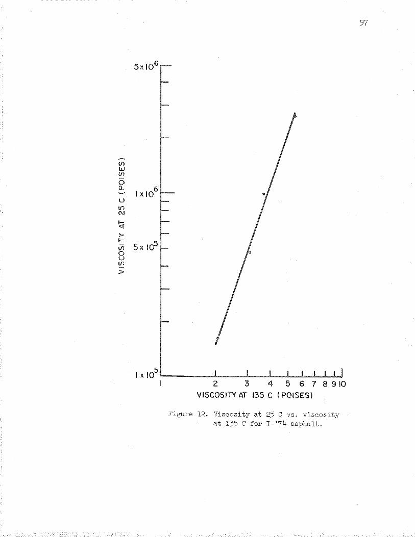
If) w If)
0 0..
1x10⁶
u !() (\j
'<! )-
'"""" 5 X 10⁵ (/)
0 u If)
>
• I
2 3 4 5 6 7 8 910 VISCOSITY AT 135 C (POISES)
Figure 12. Viscosity at 25 C vs. viscosity at 135 C for I-'74 asphalt.
97
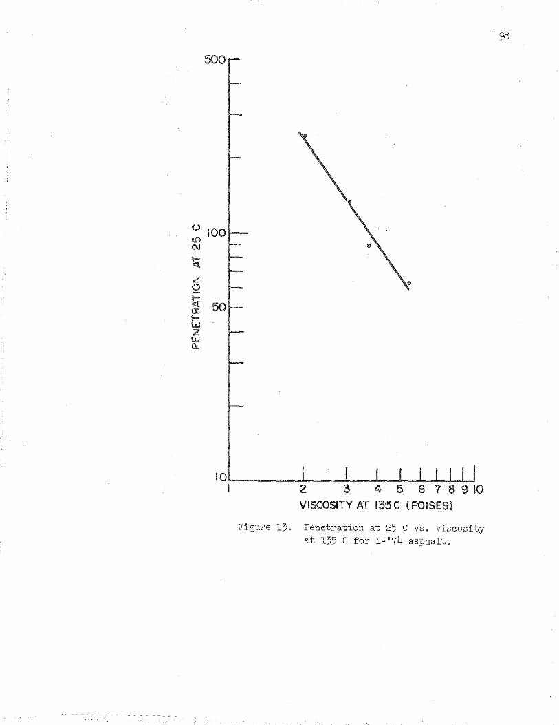
u lfl N
!;:{ z 0
~ 0: i-Ul z w Cl..
500
100
50
•
VISCOSITY AT 135C (POISES)
Figure 13. Penetration at 25 C vs. viscosity at 135 C for I-'74 asphalt.
98
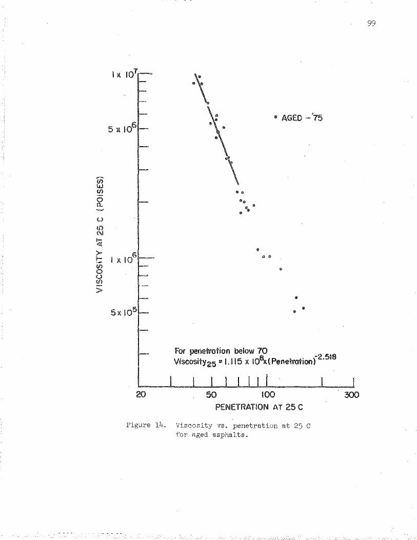
--If) w VI 0 !1. ~
u If} N
~ >-1-If) 0 u VI
>
I ll 106
• • •• ••• •
• • •
" AGED -'75
•
• •
For penetration below 70 Viscosity25 = 1.115 ll 10~( F'enetratioof
2·518
PENETRATION AT 25 C
Figure 14. Viscosity vs. penetration at 25 C for aged asphalts.
99
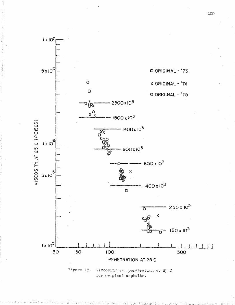
~
Vl w ~ 0 a
u !I) N
l;:i ,., 1-
Vl 0 u Vl
>
100
5xi06 0 ORIGINAL- '73
0 X ORIGINAL- '74
0 0 ORIGINAL- '75
)(
~8l!:i 2500xl03
0 X X
1800x 103
1400x 103
6 I X 10
900x 103
.......a-- 650xi03
5 ')( 5xl0
400 X 103 0
lx105 L-----~~~~~~~~----~~--~~--~~--L-~~~ 30 50 100
PENETRATION AT 25 C
Figure 15. Viscosity vs. penetration at 25 C for original asphalts.
500
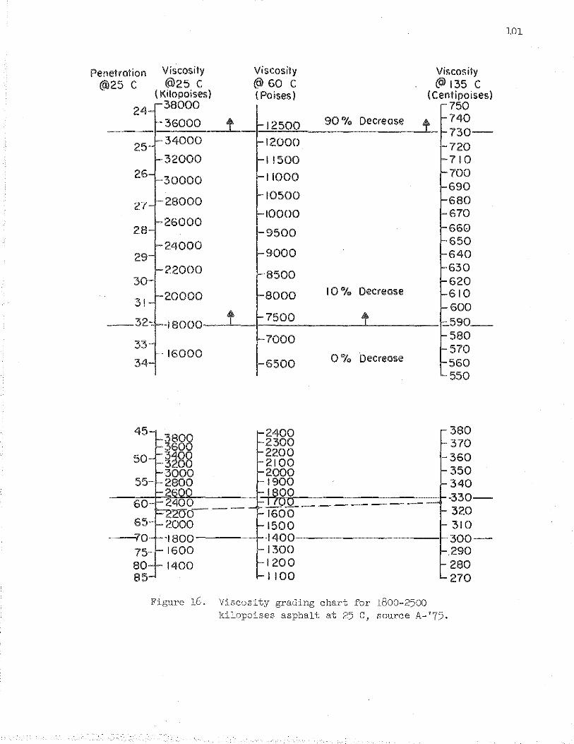
101
Penetration Viscosity Viscosity Viscosity @)25 c @25 c @) 60 c @ 135 c
( Kilopoises) (Poises l { Centipoises) 24-'38000 r750
1-36000 t i-12500 90% Decrease t 1-740 i-730-
25-i-34000 F'" 12000 1-720 t-32000 1-11500 f-71 0
26--30000 -11000 -700
-690 -28000 -10500 -680 27-
-26000 -10000 -670
28- -9500 -660
-24000 -650 29- -9000 -640
-22000 '-8500 -630
30- -620 -20000 -8000 10 "1 .. Decrease -610
31- -600 __ 32-,: --18000 f -7500 ~ -590 __
r-7000 -580 33- -570 -16000 34- -6500 0 "lo Decrease -560
-550
45 2400 380 .2300 370
50 2200 360 2100 2000 350
55 1900 340 1800 -330-
60 lfOO ---------1600 320
65 1500 310 70 •1800 ·1400 300-75 1600 1300 .290 80 1400 1200 280 85 1100 270
Figure 16. Viscosity grading chart for 1800-2500 kilopoises asphalt at 25 C, source A-'75-
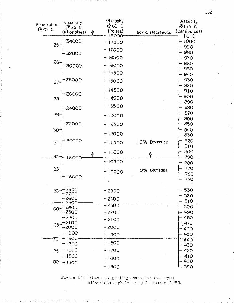
102
Penetration Viscosity Viscosity Viscosity @25 c @60 c @135 c
@25 c (Kilopoisesl + (Poises) 90% Decreos~ (Cenlipoises)
-18000 1010-
25--34000 - 17500 !- 1000
b. 990 - 17000 -980 -32000 -16500 - 970
26--16000 -960 -30000
'"""950 1-15500 !- 940
27- i-28000 -15000 i- 930 !- 920
- 14500 !- 910 1-26000
-900 28- -14000 - 890
1-24000 -13500 '"""880 29- -13000 !- 870
- 860 i-22000 - 12500 - 850
30- - 840 -1:2000 - 830
31-b. 20000
!- 11500 I 0% Decrease i- 820 !- 810
t !- 11000 1 1- 800
--32- i-18000 790-i- 10500 !- 780
33- 0% Decrease !- 770 1-10000 !- 760 i-16000 b. 750
55 2800 1"-2500 r 530 2700 1- 520 2600 1-2400 1- 510 250U 2400 1-2300 1- 500 2300 1-2200 1- 490 2200 !- 2100 !- 480 2100 1-.470 2000 i-2000 1- 460 1900 1-1900 1- 450
-70 1800 F440-1700 1- 1800 1- 430 1600 1- 1700 1- 420 1500
1- 1600 1- 410 80 1400 1- 400
L 1500 '- 390
Figure 17. Viscosity grading chart for 1800-2500 kilopoises asphalt at 25 C, source J-'75.
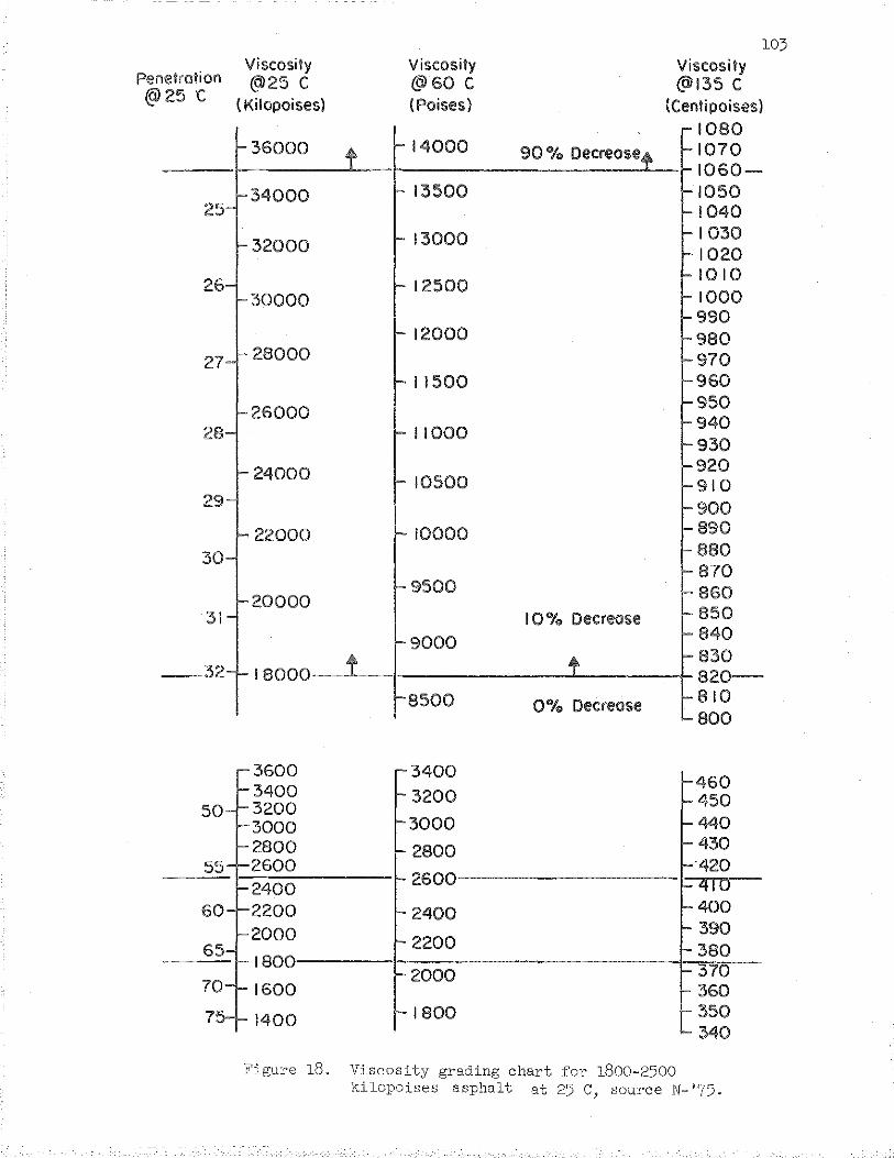
--- -- -- -
Penetration @25 c
25
26
27
28
29
30
31
--32
50-
55-
60-
65-
70-
75-
103 Viscosity Viscosity Viscosity @25 c @60 c @135 c
( Kilopoises) (Poises) (Centipoises) 1080
36000 14000 90 "/o Decrease 1070 1060-
34000 13500 1050 1040
13000 I 030 32000 1020
12500 1010 1000 30000 990
12000 980 28000 970
11500 960
26000 950 940
11000 930
24000 920 10500 910
900
22000 10000 890 880 870
9500 860 20000 850 I 0 "!., Decrease
9000 840
t 830 18000 820-
8500 0"!., Decrease 810 800
~ r 1-460 1-3400 1-3200 1-450 1-3200
3600 3400
1-3000 1-3000 1-440 1-2800 1-2800 1-430 1-2600 1-"420 1-2400
1- 2600 1-410 1-2200 1-2400 1-400
1-2000 1-390 1-2200 1-380
1-1800 1-370 t-2000 1-1600 1-360
1- 1400 r 1800 1-350 L 340
Figure 18. Viscosity grading chart for 1800-2500 ki1opoises asphalt at 25 C, source N- '75.
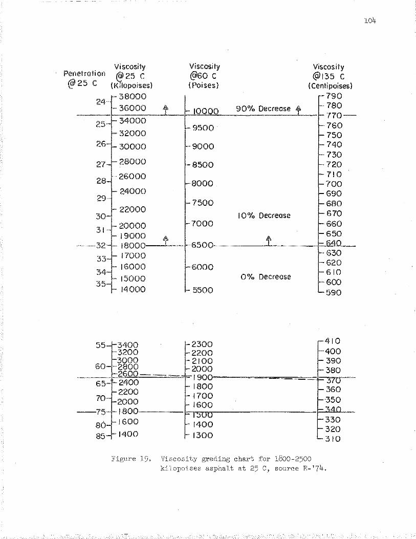
Penetration @25 c
24
25
26
27
28
29
30
31
--32
33
34
35
55
60
65
70
--75
86 85
Viscosity Viscosity Viscosity ~25 c @60 c @1135 c
( K 1lopoises) (Poises) (Centipoisesl
38000 790
36000 90% Decrease 780
34000 770-760
32000 750
30000 740 730
28000 720
26000 710 700
24000 690 680
22000 I 0% Decrease 670
20000 660 650 19000
~ 18000 6500 6~0
17000 630 620 16000 6000 610
15000 0% Decrease 600
14000 5500 590
3400 2300 410 3200 2200 400 3000 2100 390 2800 2000 380 2600----2400
1900 -- 370 1800
2200 360
2000 l700 ·350 1600
1800 340
1600 1400 330 320
1400 1300 310
Figure 19. Viscosity grading chart for 1800-2500 ki1opoises asphalt at 25 C, source E-'74.
104
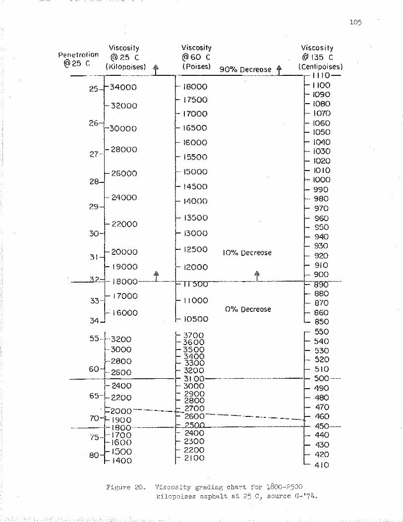
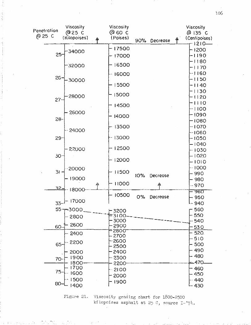
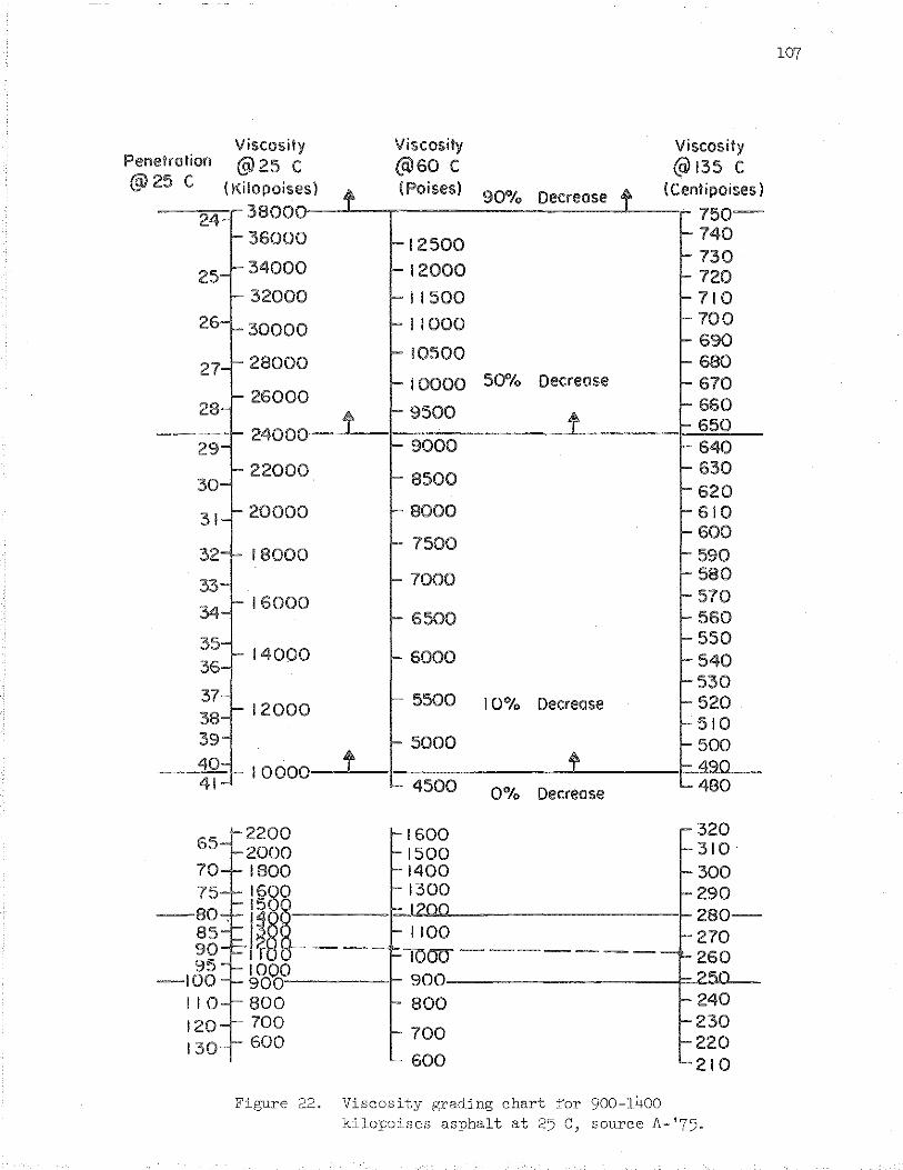
107
Viscosity Viscosity Viscosity Penetration @25 c @)60 c @135 c @25 c ( Kilopoisesl (Poises) 90"/o Decreose (Cenlipoises l
24 38000 750-36000 12500
740 130
25 34000 12000 720 32000 11500 710
26 30000 11000 700 690
28000 10500 680 27 10000 50% Decreose 670
28 26000 660
1 9500 t 650 24000 29 9000 640
22000 8500 630
30 620
31 20000 8000 610
7500 600
32 18000 590 7000 580
33 16000 570
34 6500 560 35 550
36 14000 6000 540
530 37 5500 10% Decreose 520 12000 38 510 39 5000 500 40 10000 1 ~9Q 41 4500 0% Decreose 480
2200 320 65 2000 310 70 1800 300 75 1600 290
--80, 150~ 280-
~~~ -·--85 1100 90 1000"' _______ 95 IOQO
-100 900 900 II 0 800 800 120 700
700 130 600
600
Figure 22. Viscosity grading chart for 900-1400 kilopoises asphalt at 25 c, source A-'75.
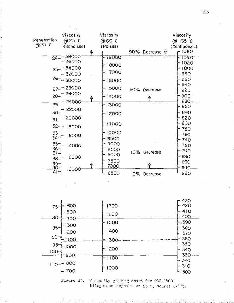
Viscosity Viscosity Viscosity Penetration @25 c (i:\)60 c (@ 135 c @!25 c ( K i lopoises) (Poises) ( Centipoises)
90"/o Decrease 1060
24 38000 36000
18000 1020 34000 1000 32000 17000 980
30000 16000 960 940
28000 15000 50"/., Decrease 920 26000
14000 900.
24000 880-13000 860
22000 840 12000
20000 820 11000 800
18000 780 16000
10000 760 9500 740
14000 9000 720 8500
I 0"/o Decrease 700
12000 8000 680 7500 660
10000 7000 640-6500 0% Decrease 620
-430 1-1700 -420
--80 1500 ~ 410
1- 1600 4(')(') 1400----~~---------------~~~-
!- 380 1200 1- 1400 ,__ 370
85 I- 1500 !- .390
1300
90 :llill)___ 1- 1300---------1- 360 ..--r r 350
10oo ~ 1200 r- 340 100
95
---+- 900 330-~ 1100 r- 320
110 1- 310 800
~1000 700 '-300
Figure 23. Viscosity grading chart for 900-1400 ki1opoises asphalt at 25 C, source J- '75·
108
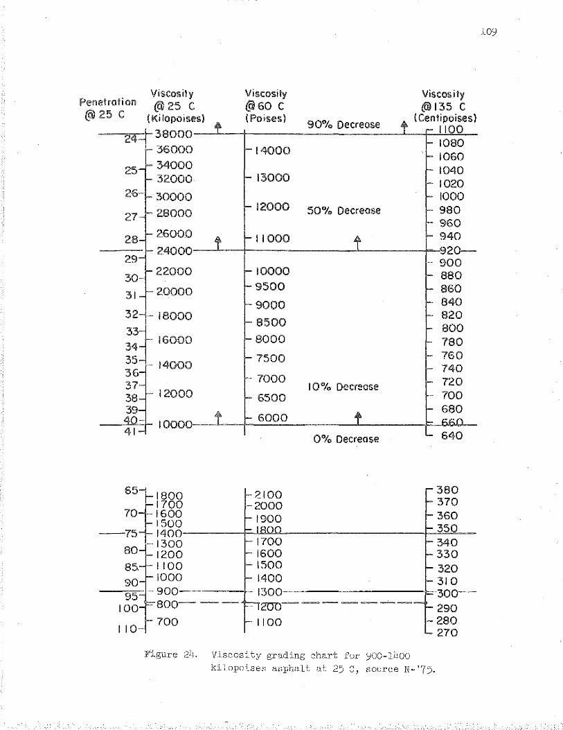
Penetrol ion @25 c
24
25
26
27
28
29
31
65
70
--75
80
110
Viscosity Viscosity Viscosity @125 c @60 c (.6)135 c
( Ki lopoisesl (Poises) 90"/o Decrease
( Centipoisesl 1100 38000 1080
36000 14000 1060
34000 1040 32000 13000 1020 30000 1000
28000 12000 50% Decrease 980
960 26000 I 1000 940 24000 920-
22000 10000 900 880
20000 9500 860
9000 840 18000 820
8500 800 16000 8000 780
7500 760 14000 740
7000 I 0% Decrease 720
12000 6500
10000 6000
0% Decrease
Figure 24. Viscosity grading chart for )100-1400
kilopoises asphalt at 25 C, source N- '75.
109
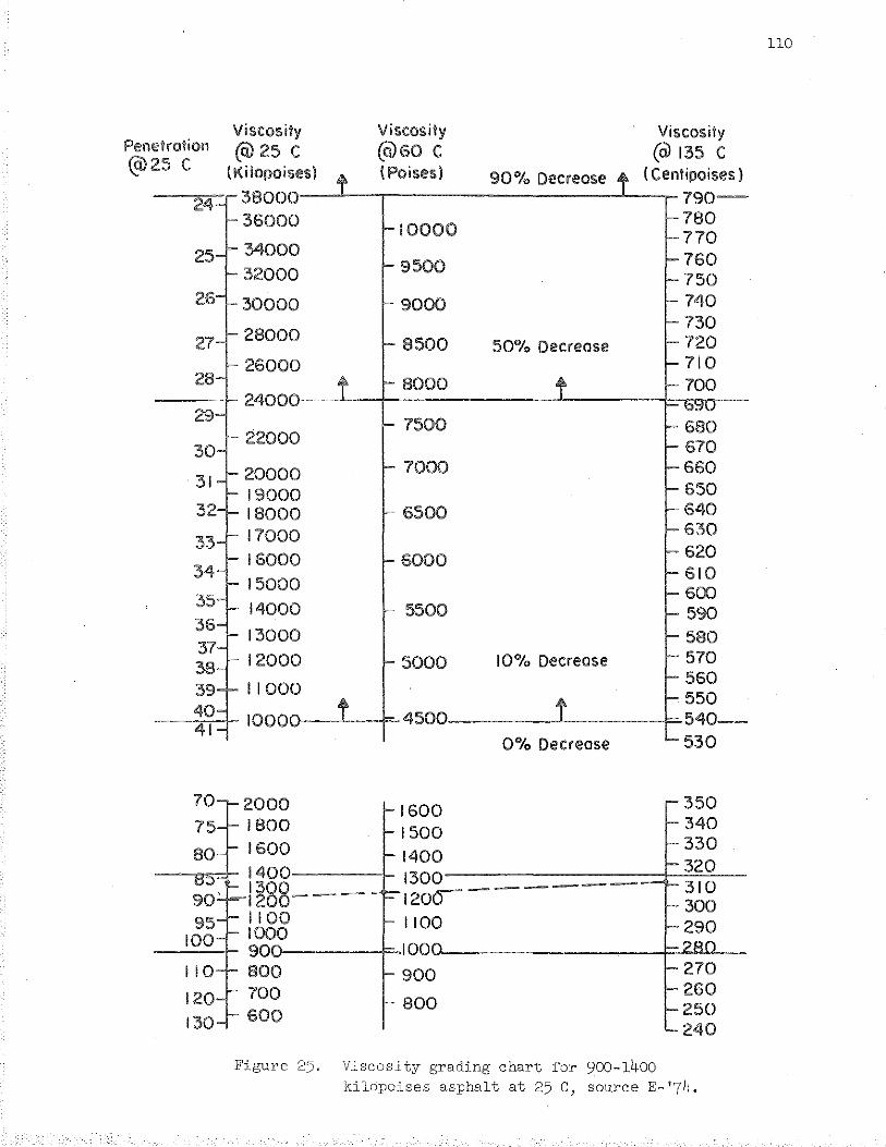
Penetration @25 c
24
25
27
28
29
Viscosity Viscosity Viscosity (ci) 25 c @)60 c @ 135 c
(Kilopoisesl I Poises) 90% Decrease ( Centipoises) 38000 790-36000 10000
780 770
34000 32000 9500
30000 9000
28000 8500 50% Decrease
26000 8000
22000 7500
20000 1000
19000 18000 6500 17000 16000 6000 15000
14000 5500 13000 580 12000 5000 10% Decrease 570
11000 560 550
1000 4500 540-
0% Decrease
2000 1600 1800 1500 1600 1400 1400 1300 1~88--- 1200------II 00 1100 1000 900 100 800 900 700
800 600
Figure 25. Viscosity grading chart for 900-1400 kilopoises asphalt at 25 c, source E-'74.
llO
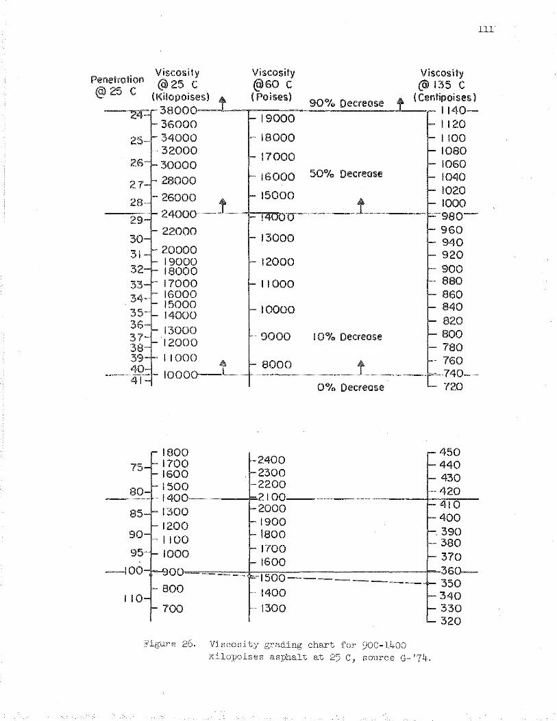
lll
Penetration Viscosity Viscosity Viscosity
@ 25 c @25 c @60 c @) 135 c (Kilopoisesl (Poises) ( Centipoises l
38000 90"/o Decrease
1140-24 19000 36000 1120
25 34000 18000 1100 32000
17000 1080 26 30000 1060
28000 16000 50"/., Decrease 1040 27 1020 28 26000 15000
1000
29 24000 980-
22000 960 30 13000 940 31 20000 920
19000 12000 32 18000 900
33 17000 11000 880
34 16000 860 15000 10000 840
35 14000 820 36 37
13000 9000 I 0% Oecreose 800
38 12000 780 39 11000
8000 760 40 1000 740-41
0% Decrease 720
1800 ,..... 450
75 1700 ~2400 1-440 1600 1-2300 f- 430
80 1500 1-2200 1-420
1400 2100 f- 410
1300 1-2000 85 f-400 1200 1- 1900
90 1- 1800 1-. 390 1100 1-380
95 1000 1- 1700 1- 370 1- 1600
-100 00 1="1500---------
360--1- 350
110 1- 1400 1-340 700 1- 1300 f- 330
'-- 320
Figure 26. Viscosity grading chart for 900-1400 kilopoises asphalt at 25 C, source G- '7le.
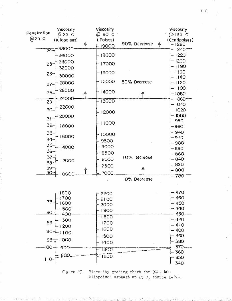
112
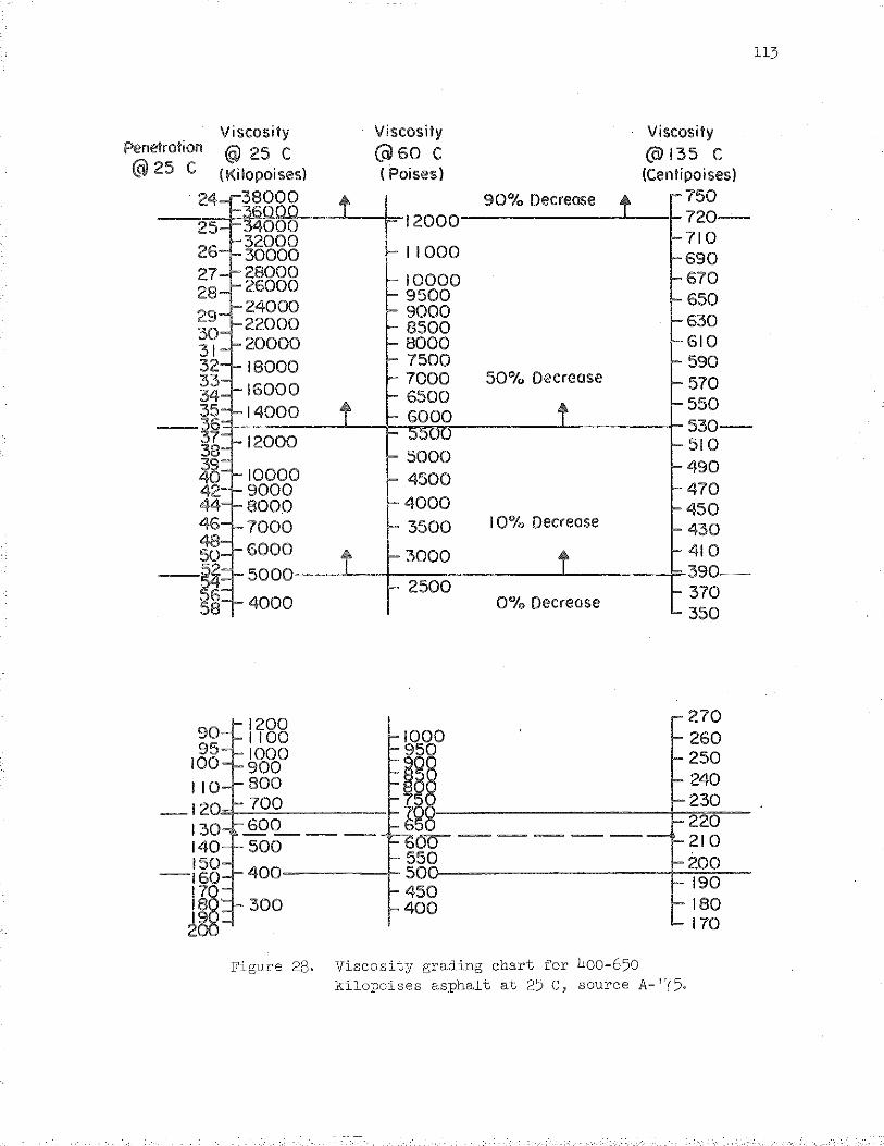
113
Penetration Viscosity Viscosity Viscosity @ 25 c @60 c @1135 c
@25 c (Kilopoisesl (Poises) (Cenlipoisesl
24 38000 90% Decrease t 750
25 4000 12000 720-32000 710
26 30000 11000 690 27 28000 10000 670 28 26000 9500
24000 650 29 9000 30
22000 8500 630
31 20000 8000 610 32 18000 7500 590 33 16000
7000 50% Decrease 570 34 6500 35 14000 6000
550
-~~ 530-12000 510 38 5000 4o 10000 4500
490 42 9000 470 44 800.0 4000 450 46 7000 3500 I 0% Decrease 430 48 6000 410 50 3000
-~ 390-2500 370 56 0% Decrease 58 350
1200 270 90 1100 1000 260 95 1000 95 250 100 900 -i 110 800 240
_120 700 230
130 600 220 ---- oo----- 210 140 500
150 550 200 -160 400 50
190
l~ 450
300 400 180 170
Figure 28. Viscosity grading chart for 400-650 kilopoises asphalt at 25 C, source A-'75.
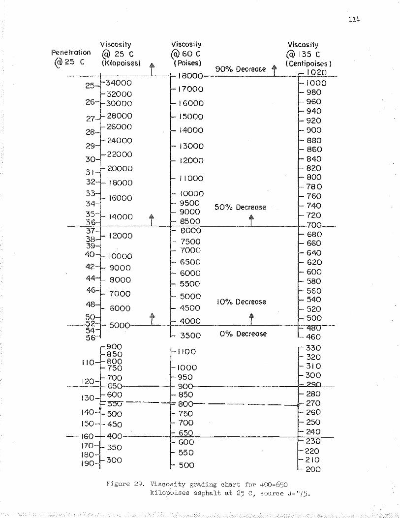
114
Viscosity Viscosity Viscosity Penetration (Q) 25 c @)60 c (ci) 135 c @25 c (Kilopoisesl (Poises)
90% Decrease ( centipoises )
1020 18000
32000 17000
1000 980
30000 16000 960
28000 940 15000 920
26000 14000 900 24000 880
13000 860 22000 840 12000
20000 820 11000 800
18000 780 16000 10000 760
9500 50% Decrease 740 14000
9000 720 8500 700-
12000 8000 680 7500 660 7000 640 10000 6500 620
9000 6000 600
8000 5500 580
7000 560 5000
I 0"/o Decrease 540 6000 4.500 520
4000 500 5000
3500 0% Decrease
900 1100 850
110 800 750 1000
120 700 950 65 900
130 600 850 55CT-- 8oo----- ---
140 500 750 150 450 700
--160 400- 650
170 600 350
180 550 190 300
500
Figure 29. Viscosity grading chart for 400-650 kilopoises asphalt at 25 c, source J-'75.
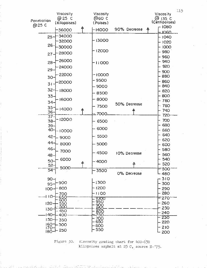
115 Viscosity Viscosity Viscosity
Penetration @25 c @)60 c @ 135 c ( Kilopoises) (Poises l (Cenlipoises)
@25 c 90'% Decrease
1080 36000 14000
34000 1040 32000 13000 1020 30000 1000
28000 12000 980
960 26000 11000 940 24000 920
22000 10000 900 880
20000 9500 860 9000 840
18000 8500 820
800 16000 8000 780
7500 50'%, Decrease 760 14000 740
700 720-12000 6500 700
680 10000
6000 660
5500 640 9000
620 8000 5000 600
7000 580 4500 I 0% Decrease 560
6000 4000 540 520
5000 3500 soo-
0'% Decrease 480 90 310 95" 900 300
100 800 1200 290 700 280
~88 270-950 260 120 550 900
130 ~-- 850-- ------ -- 250 450 800 240 -140 400 750
230 150 700 350 650 220 160 300 600 210 170 180 250 550
200
Figure 30. Viscosity grading chart for 400-650 kilopoises asphalt at 25 C, source N- '75.
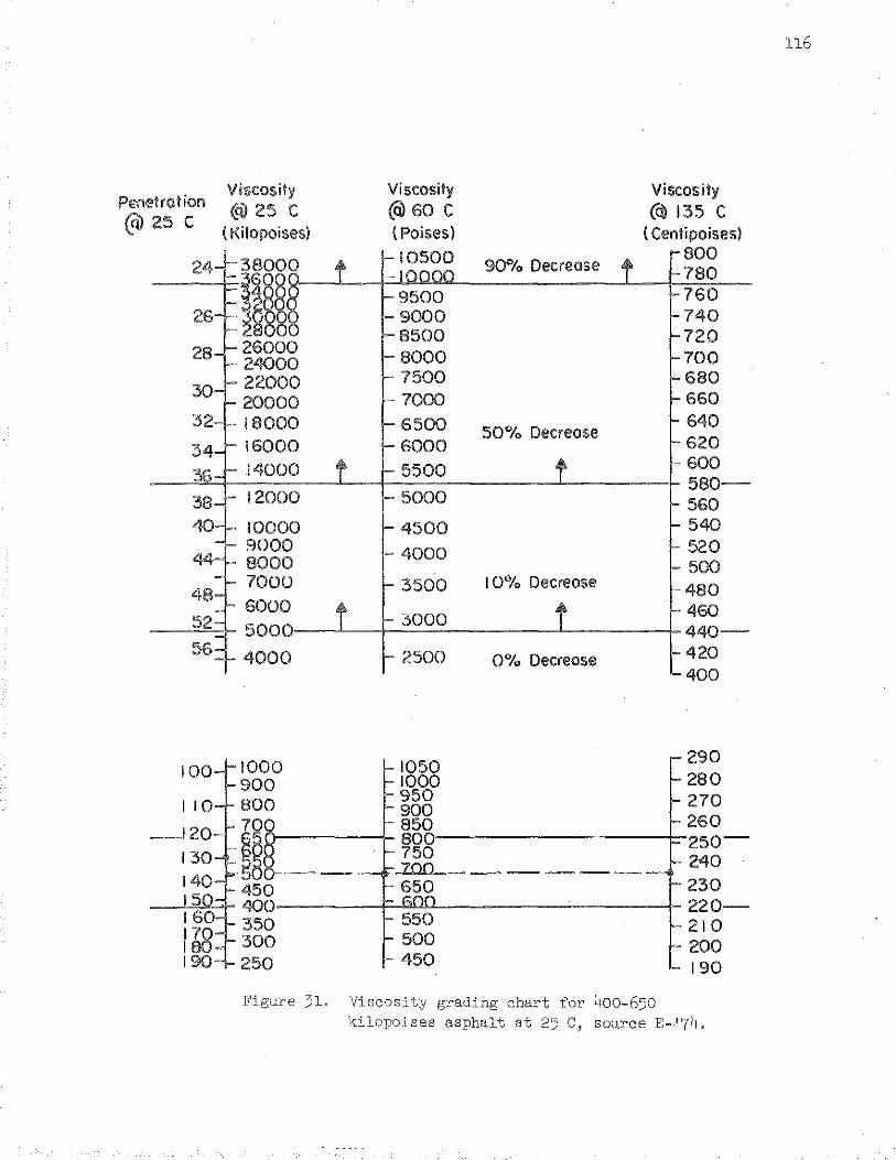
Penetration Viscosity Viscosity Viscosity @ 25 c @)60 c (Q) 135 c
@l25 c ( Kilopoises) (Poises) ( Centipoises) 10500 800
38000 90% Decreose 780
i§~~~ 9500 760 9000 740 8500 720
26000 8000 700 24000
22000 7500 680 20000 660 18000 50% Decreose
640 16000 620
14000 600 580-
12000 560 10000 4500 540 9000 4000 520 8000 500 7000 3500 I 0% Decrease 480 6000
3000 460 5000 440-
4000 2500 0% Decrease 420 400
r- 290 1000 r-1050 1-280 900 1-1000 800 ~ §68 1- 270
~B0 __ -· _: !~§~-----------!::-: ~ig-~go r- §~Q -----·-~-- 230
--'->~>j- 400 1- o-.r ll I 22 0-350 1- 550 1- 2 I 0 300 1- 500 1- 200 250 1- 450 '- I 90
Figure 31. Viscosity grading chart for 400-650 kilopoises asphalt at 25 c, source E-'74.
116
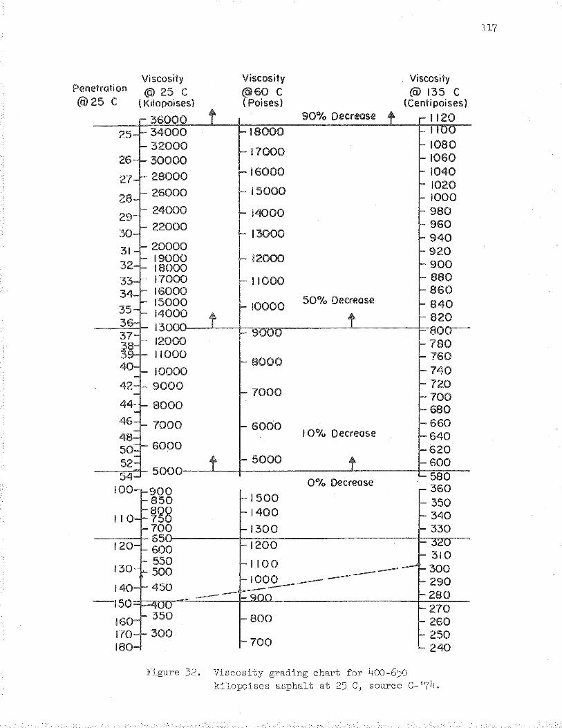
117
Viscosity Viscosity Viscosity Penetration @ 25 c @60 c (ci) 135 c (cil25 c ( Kilopoisesl l Poises) (Centipoises)
36000 90''/o Decrease 1120 34000 18000 32000 17000
1080
30000 1060
28000 16000 1040
26000 15000 1020 1000
24000 14000 980 22000 960
13000 940 20000 920 19000 12000 900 18000 17000 11000 880 16000 860 15000 10000
50'%, Decreose 840 14000 820 130 8oo-
180 760
10000 42 9000
8000
1000 660 I 0% Decrease 640
6000 620 600
5000 580 0% Decrease 900 360 850 1500 350 8~0 1400 340 110 7 0 700 1300 330
120 65
1200 600 550 310
130 500 -- 300 - 290 140 450 - 280
-150 270 160 350 260 170 300 250 180 240
Figure 32. Viscosity grading chart for 400-650 kilop0ises asphalt at 25 c, source G-t74.
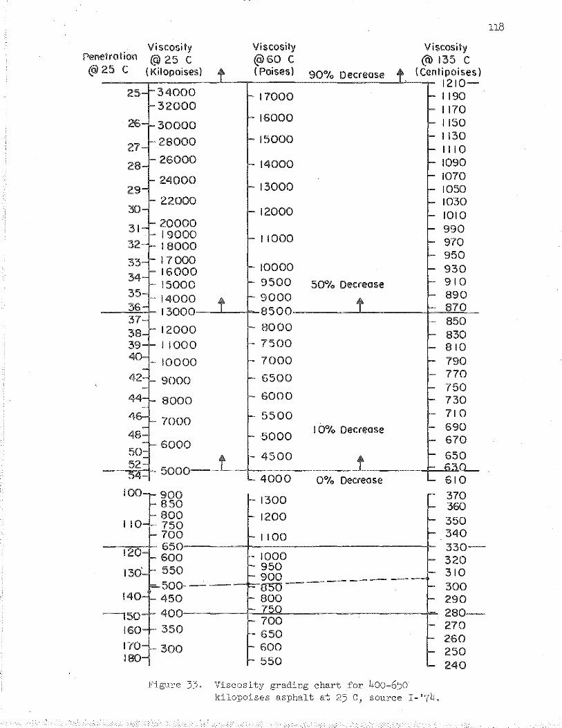
118
Penel r o I ion Viscosity Viscosity Viscosity @) 25 c @60 c @> 135 c
@25 c ( Kilopoises) (Poises) 90% Oecreose (Centipoises) 1210-
34000 17000 1190 32000 1170
30000 16000 1150
28000 15000 1130 1110
26000 14000 1090
24000 1070 13000 1050
22000 1030 12000 1010
20000 990 19000 11000 970 18000 17000 950
16000 10000 930
15000 9500 50'% Decrease 910
14000 9000 890
13000 8500 870
8000 850 12000 830 11000 7500 810 10000 7000 790
9000 6500 770 750
8000 6000 730 5500 710
7000 5000
I 0% Decrease 6000
4500 5000
4000 0% Decrease 900 1300 370 850 360 800 1200 350 750 700 1100 340 650 330-600 1000 320 550 950 310 900 -----500--- gso- 300
140 450 800 290
~50 400 280-
160 350 270 260
170 300 250 100 550 240
Figure 33. Viscosity grading chart for 400-6)0 kilopoises asphalt at 25 c, source I-'74.
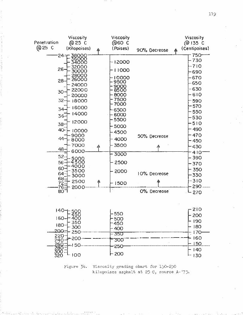
ll9
Viscosity Viscosity Viscosity Penel rolion @) 25 c (@60 c (a) 135 c @25 c (Kilopoisesl (Poises) 90% Decrease ( Centipoisesl
~~§§§ 750-
12000 730 32000 710 30000 11000 690 28000 10000 670 26000 24000
9500 650 22000 ~~88 630 20000 8000 610 18000 7500 590
7000 570 16000 6500 550 14000 6000 5500 530
12000 510 5000
490 10000 4500 9000 50"/o Decreose 470 8000 4000 450 7000 3500 430 6000
3000 410-
4000 390 500 2500 370
60 4000 350 3500 2000 64 3000 I 0% Decrease 330
68 2500 310 72 1500
--76 200 290-80 0% Decrease 270
r- 210 4~8 1- 550 1- 200 400 1- 500 1- 190
~gg ~:gg 1- 180 -2-Ltu..:::J.- 250 1- 350 . I 7D--
200-- ----b-,,.,o----- ----p.. 160
I 50 .:5U' 1- I 50
-~~!=- 25U
100
}"igure 34-
1-200 1- 140 1- 130
Viscosity grading chart for 150-250 kilopoises asphalt at 25 C, source A- '75-
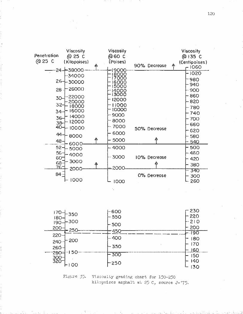
Viscosity Penetration @) 25 c @l25 c ( Kilopoises)
38000 34000 30000
26000
22000 20000 18000 16000 14000 12000 10000
8000
6000 5000 4000 3000
2000
1000
Viscosity @60 c (Poises)
19000 18000 17000 16000 15000 14000 13000 12000 11000 10000 9000 8000 7000 6000
5000
4000
3000
2000
1000
f-600 1-550
90% Decrease
50"1., Decrease
I 0"/., Decrease
0% Decrease
Viscosity (00 135 c
{Cenlipoises) 1060 1020
780 740 700 660 620 580 540 500 460
•230 1-220 -210
-500 -200 ---=-=-;t,-2~- -·-~ 45_v _______ ._;-·l90
240 260
-2a 300 320
200 -400 - 180 -350 - 170
15v0-~--------+-~~-------------------t-~16~0~--300 - 150
100 1-250 1- 140 ~ 130
Figure 35. Viscosity grading chart for 150-250 kilopoises asphalt at 25 C, source J-'75.
120
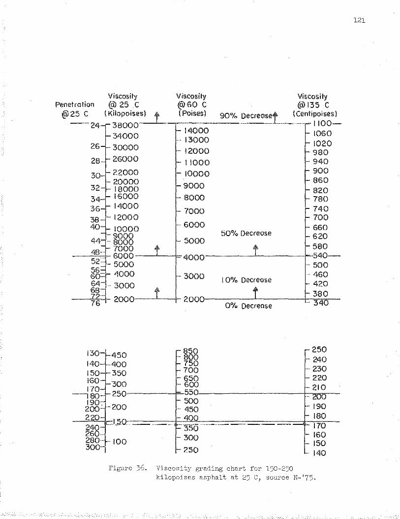
Penetration @25 c
--24
26
130 140 150 160 170
-180 190. 200 220 240 260 280 300
Viscosity Viscosity Viscosity @ 25 c @60 c @) 135 c
( Kilopoises) (Poises) 90% Decrease (Centipoises)
38000 1100-
34000 14000 1060 13000 1020 30000 12000 980
26000 11000 940 22000 10000 900 20000 860 18000 9000
820 16000 8000 780 14000
7000 740 12000 700
10000 6000 660 9000 50% Decrease 620 8000 5000
580 7000 6000 4000 540-5000 500 4000 3000 460
I 0% Decrease 420 3000 380
2000 200 340 0% Decrease
450 850 800
400 750 350 700
650 300 600 250 550
200 500 450
I !ill= ----400 350 ______
100 300
250
Figure 36. Viscosity grading chart for 150-250 kilopoises asphalt at 25 C, source N-'75.
121
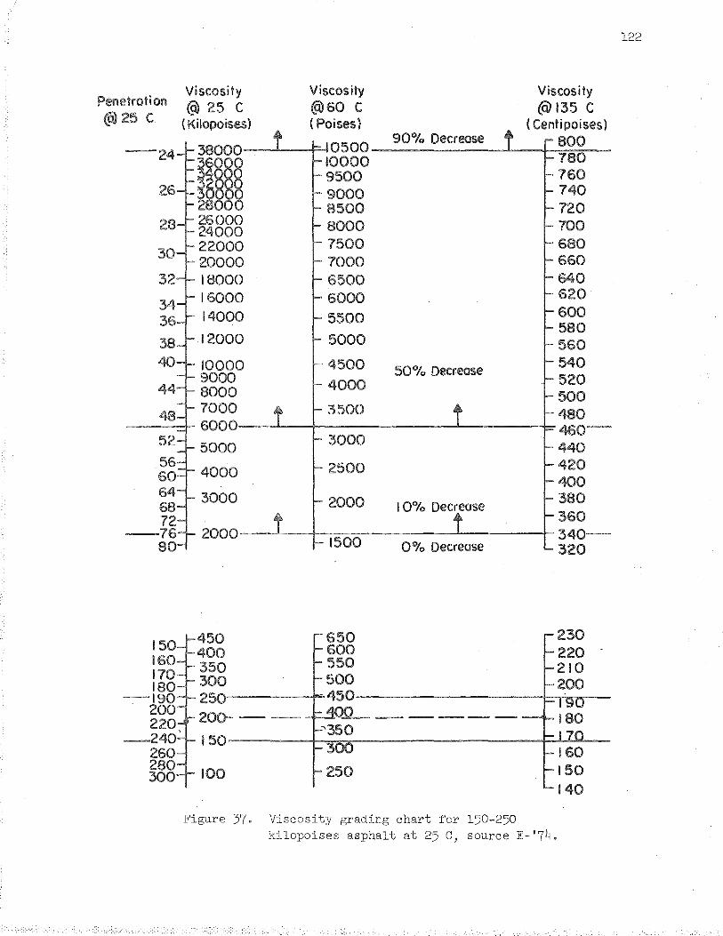
Penetration @25 c
--24
26
28
30
32
34 36
38 40
44
48
52
56 60 64 68 72
--76 80
150 160 170 180
-190 . 200
220 -240
260 280 300
Viscosity Viscosity @ 25 c @)60 c
( Kilopoise.sl (Poises)
38000 10500
~~~~ 10000 9500 9000 8500
26000 8000 24000 22000 7500 20000 7000 18000 6500 16000 6000 14000 5500
12000 5000
10000 4500 9000 4000 8000 7000 3500 6000
5000 3000
4000 2500
3000 2000
2000 1500
450 400 350 300 250>----.....jc,
Viscosity @J 135 c
( Cenlipoises) 90% Decrease BOO
780 760 740 720 700 680 660 640 620 600 580 560
50% Decrease 540 520 500 480 460-440 420 400 380 I 0% Decrease 360 340-
0% Decrease 320
20Q- - ---i~~- -- ------ --
150--------~~~----------------~~~-
100
Figure 37. Viscosity grading chart for 150-250 kilopoises asphalt at 25 c, source E-'74.
122
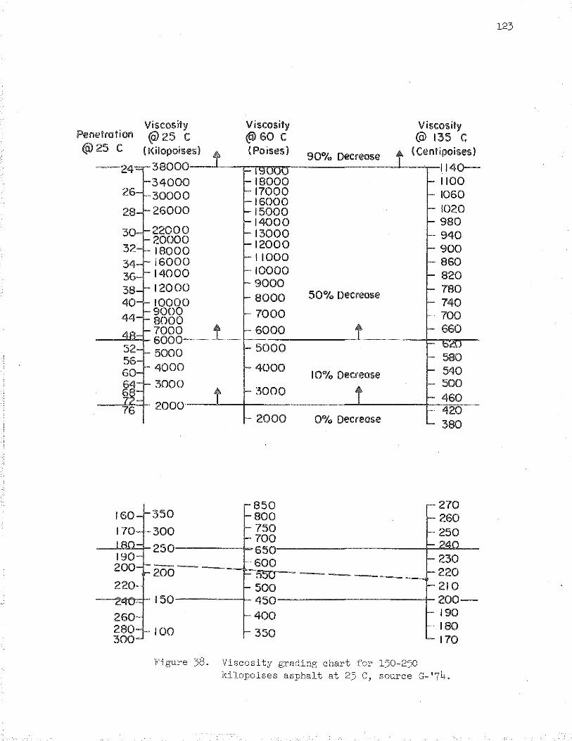
PenelmtiOil @25 c
Viscosity Viscosity Viscosity (@ 25 c (6)60 c (OJ 135 c
( Kilopoisesl (Poises) 90"/o Decreose ( Centipoises)
38000 114()--34000 18000 1100 30000 17000 1060
16000 26000 15000 1020
14000 980 22000 13000 940 20000 12000 900 18000 16000 11000 860 14000 10000 820 12000 9000 780 10000 8000 50% Decreose
9000 7000 8000 7000 6000 6000
5000 5000 4000 4000
I 0"/., Decreose 3000
3000 460
2000 420 2000 0"/o Decrease 380
850 350 800 300 750
700 250 650
600 230 200-- 550 ---- 220
500 210 150 450 200-
400 190
100 350 180 170
Figure 38. Viscosity grading chart for 150-250 kilopoises asphalt at 25 C, source G-'74.
123
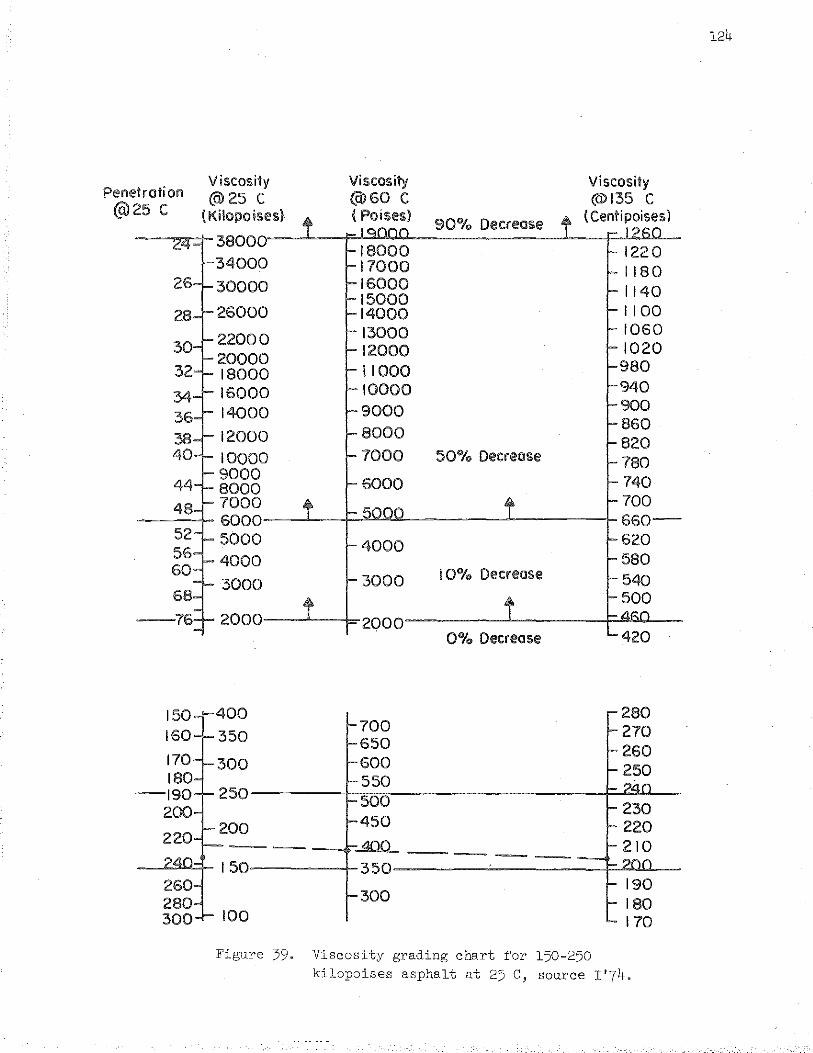
Penetration @25 c
26
28
30
32
34 36 38 40
44
68
170 180
-J90 200
Viscosity @125 c
(Kilopoises)
3800 34000
30000
26000
22000 20000 18000 16000 14000
12000 10000 9000 8000 7000 6000 5000 4000
3000
2000
Viscosity @>60 c (Poises)
18000 17000 16000 15000 14000 13000 12000 11000 10000 9000 8000
7000
6000
4000
3000
2000
700 650 600 550 500 450
90% Decrease
50% Decrease
I 0% Decrease
0"/o Decrease
Viscosity (li) 135 c
( Centipoisesl
1180 1140 1100 1060 1020 980 940 900 860 820 780 740 700 660-620 580 540 500
-- -- -4"":..!40!1.J.1..0L _____ _
--~~ 150t-------~350-------~-------~~~-
300 100
180 170
Figure 39. Viscosity grading chart for 150-250 kilopoises asphalt at 25 c, source 1'74.
124
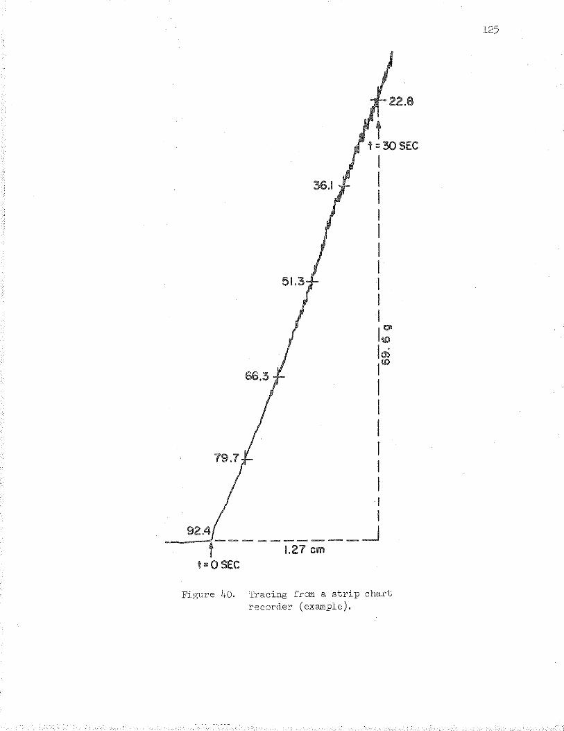
79.7
t t = 30 SEC
I I I I I I I I I I 1: lm liD
I I I I I I I I
92.4 _j t--- --1.""27 ~--
t= 0 SEC
Figure 40. Tracing from a stri.P chart recorder (example).
125
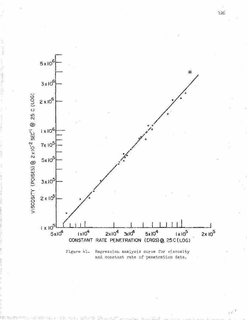
(.!)
0 _J ~
u 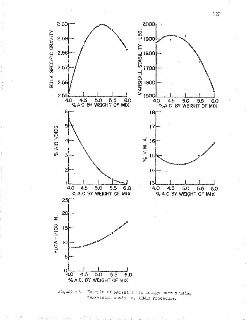
/~' . \
•
2.55• I
z
8 ' I 3: 0 ...J. lL
4.0 4.5 5.0 5.5 6.0 %A.C. BY WEIGHT OF MIX
4.0 4.5 5.0 5.5 6.0 "lo A.C. BY WEIGHT OF MIX
127
<( 16 •
~15·~ ~/ ~ ./ @ .~
14
13~--~--~--~~ 4.0 4.5 5.0 5.5 6.0
%A.C.8Y WEIGHT OF MIX
Figure 42. Example of Marshall mix design curves using regression a.na.lysis, AIMIX procedure.
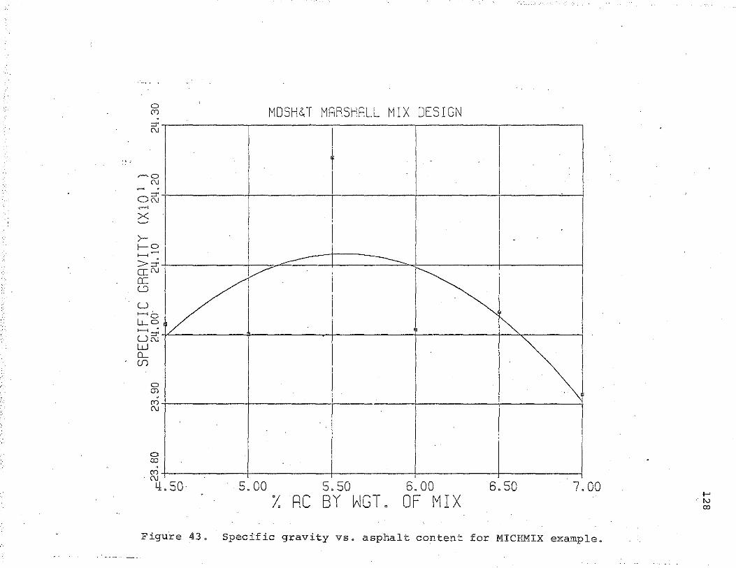
:·'
0 (C) . :::r (\]
~o (\] - .
0~ ....... X
>-r---s >---< >;;:i< O::N a: C)
u >---<(:) i..LO >--; •
u~ w n_ (f)
0 0)
(C) (\]
0 (XJ
('f) . (\]
MOSH&T MARSHALL MIX DESIGN
I
----- --------
./ v
~ ~
I
' 4.50 5.00 5.50 6.00 6.50
% RC BY HGT" OF MIX
I
I
7.00
Figure 43. Specific gravity vs. asphalt content for MICHMIX example.
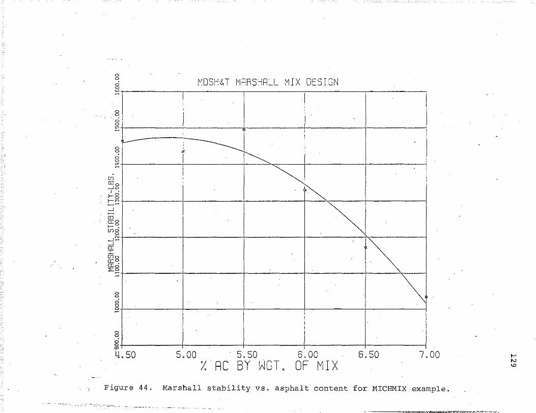
. . ·~ .... ~-.
0 0
0 0
"'
0 0
0 0
"'
0 0
0 0
""
0 0
0 g
g
I ,_
.
g 4.50
MDSH&T MRRSHRLL MIX DESIGN
I I
-----------~ .
~ ~
~ ~ ~
5.00 5.50 6.00 6.50 7.00 % RC BY WGT. OF MIX
Figure 44. Marshall stability vs. asphalt content for MICHMIX example .
.--.-.-._._. ______ -- ··-------
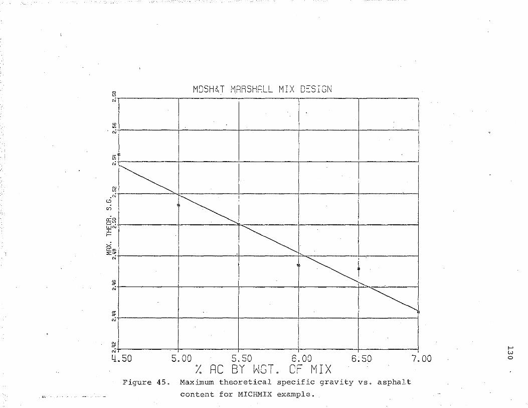
a:g D. WN I ,_
~ I
~
MOSH&T MRRSHRLL MIX DESIGN
~ .~ ~ :-.... ~
4.50 5.00 5.50 6.00 6;50 7.00 % RC BY HGT. OF MIX
Figure 45. Maximum theoretical specific gravity vs. asphalt
content for MICHMIX example.
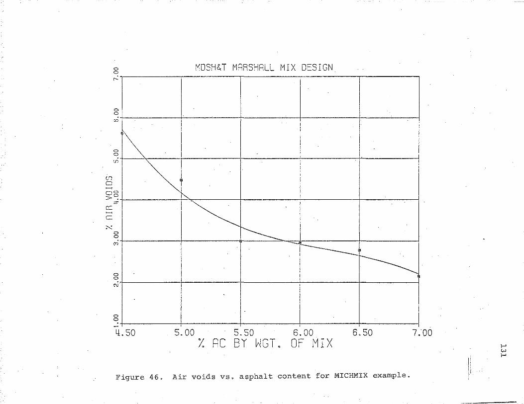
(f) 0
a:
0 0
r-
0 0
.r\ 0 0
0 0
"'
0 0
N
0 0
I
I I I '
I I
4.50
MOSH&T MRRSHRLL MIX DESIGN
I I
~ I
I~ '------- -~
~·
5.00 5.50 6.00 6.50 7.00 % RC BY WGT. OF MIX
Figure 46. Air voids vs. asphalt content for MICHMIX example.
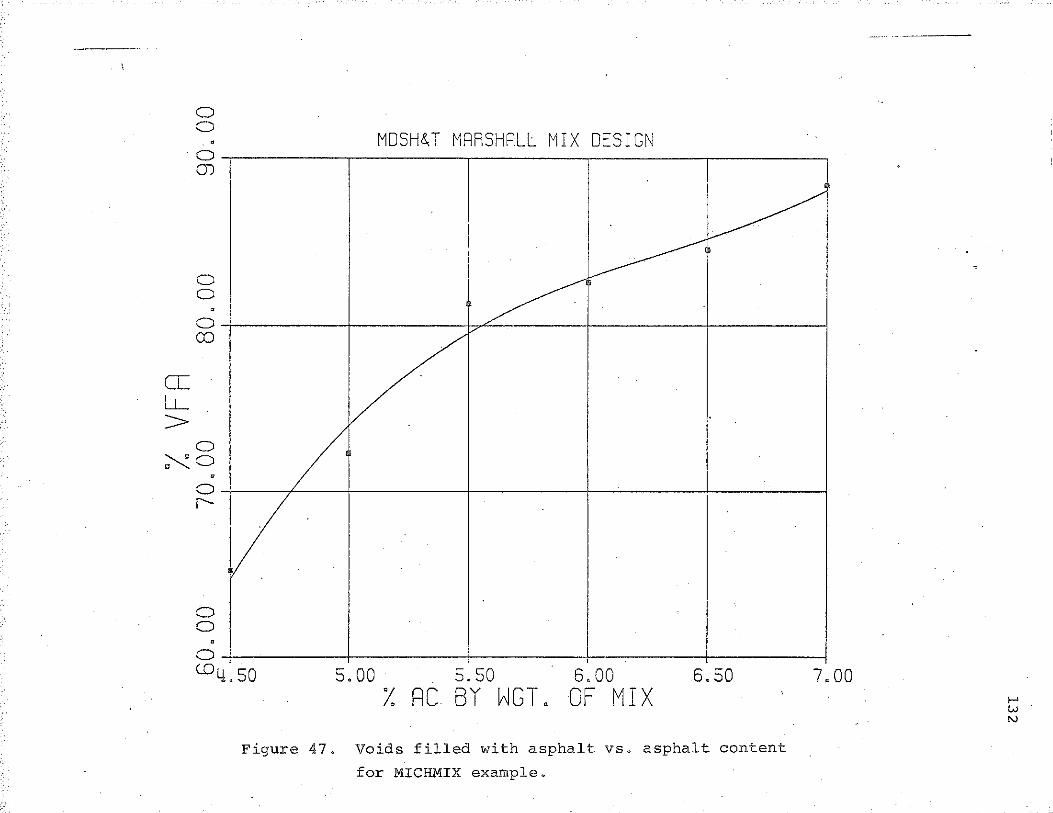
cr:: LL >
0 0
0 m
0 0
0 CD
0 ~0
0 r--
MDSH~T MRRSHRLL MIX DESIGN
~ ~
~
/ I ' '
5. 00 . 5. 50 6.00 6.50 /. RC BY NGT. OF MIX
Figure 47. Voids filled with asphalt vs. asphalt content
for MICHMIX example.
7.00 1-' w N
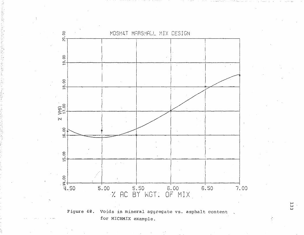
0 0
0 N
0 0
en -0 0
00 -
0 0
"' -0 0
tJ) -0 0
r-----
-
MDSH&T MARSHALL MIX DESIGN
~
/ v
I
~ v
I
4.50 5.00 5.50 6.00 6.50 7.00 I. RC BY WGT. OF MIX
Figure 48. Voids in mineral aggregate vs. asphalt content
for MICHMIX example.
1-' w w
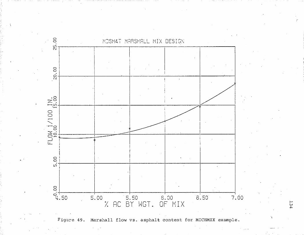
..
0 0
L0 (\J
0 0
0 (\J
.o :z:C: ,_.\.f) ·-0 0
..-.o 0
::;:: . o:=: _j
LL
0 0 . \.f)
0 0
0
I I
I
I
!
L!.SO .
MOSH&T MARSHALL MIX DESIGN
. / ~~
~ ....... I
I
s.oo ·s.so 6.00 6.50 7.00 /. RC BY WGT. OF MIX
Figure 49. Marshall flow vs. asphalt content for MICHMIX example. \
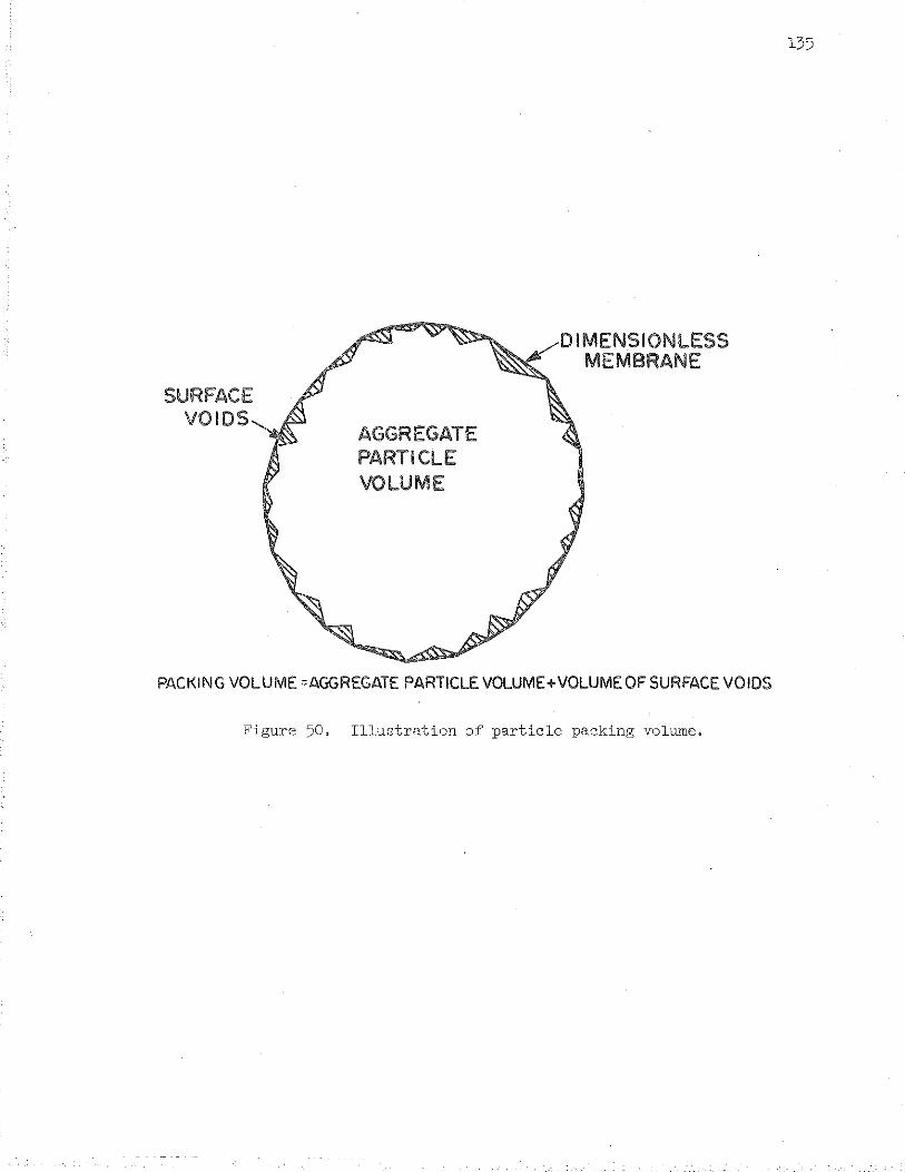
SURFACE VOIDS
AGGREGATE PARTICLE VOLUME
./DIMENSIONLESS Jill' MEMBRANE
PACKING VOLUME =AGGREGATE PARTICLE VOLUME+VOLUMEOF SURFACE VOIDS
Figure 50. Illustration of particle packing volume.
135
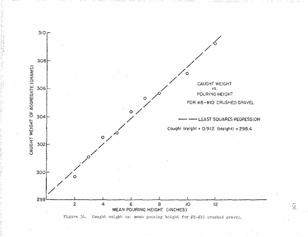
<f)
::1: <1: 0::: <.::>
310
308
w 306 ~ ti3 0::: <.::> <.::> <1: IJ.. 0 304 1--:I: C> w 5: I-
~ 302 ::::J <1: u
300
CAUGHT WEIGHT vs.
POURING HEIGHT
FOR #8-#10 CRUSHED GRAVEL
--LEAST SQUARES REGRESSION
Caught Weigh! = 0.912 (Height} + 298.4
298~------~------~------~------~------~------L--------------2 4 6 8 10 12
MEAN POURING HEIGHT {INCHES)
Figure 5l. Caught weight vs. mean pouring height for #8-#lO crushed gravel.
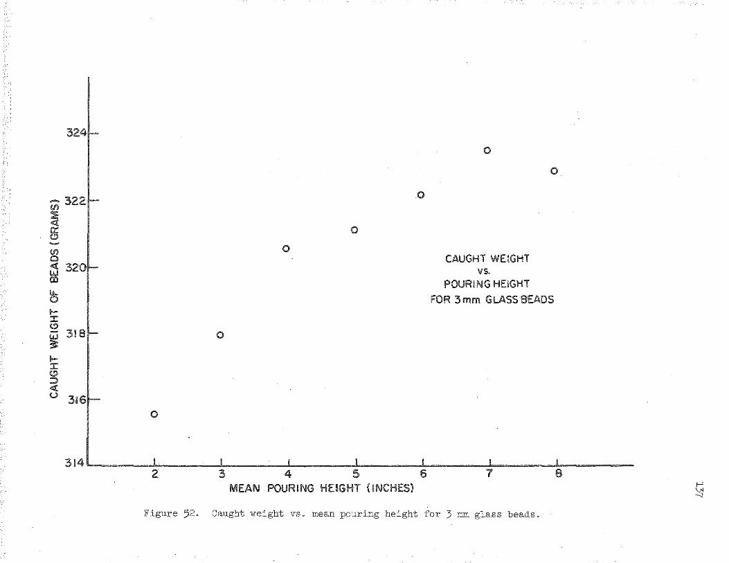
324
-322 !f)
:::E <t !li: C) ~
!f) 0 <t 320 IJJ Ill IJ.. 0 i-J: C)
318 IJJ 31: i-:;: C) :::;) <t u 316
.0
0
0
0
0
0
CAUGHT WEIGHT 1/S.
POURING HEIGHT
0
FOR 3 mm GLASS BEADS
314L-------~-------L------~------~~------~------~------~---------2 3 4 5 6 7 8
MEAN POURING HEIGHT {INCHES)
Figure 52. Caught weight vs. mean pouring height for 3 mm glass beads.
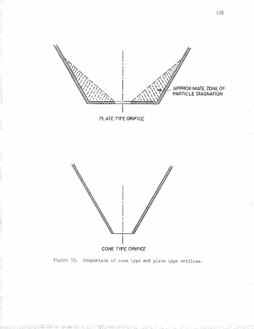
PLATE TYPE ORIFICE
CONE TYPE ORIFICE
138
~IS'- APPROXIMATE ZONE OF PARTICLE STAGNATION
Figure 53. Comparison of cone type and plate type orifices.
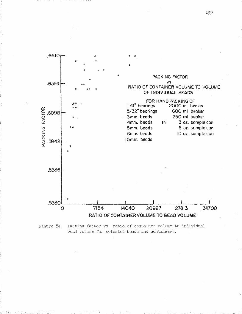
.6610
·6354
!lC ~ .6098 u ~ <.') 2
~
~ .5842 a.
. 5586
•
•
• • •
•• •
,. . ••
•
••
•
139
• • • •
• • '
• • PACKING FACTOR
\1 s.
•• • RATIO OF CONTAINER VOLUME TO VOLUME OF INDIVIDUAL BEADS
FOR HAND PACKING OF 1/4" bearings 2000 ml beaker 5/32" bearings 600 ml beaker 3mm. beads 250 ml beaker 4mm. beads IN 3 oz. sample con 5mm. beads 6 oz. sample can 6mm. beads I 0 oz. sample can
15mm. beads
RATIO OF CONTAINER VOLUME TO BEAD VOlUME
Figure 54. Packing factor vs. ratio of container volume to individual bead volume for selected beads and containers.
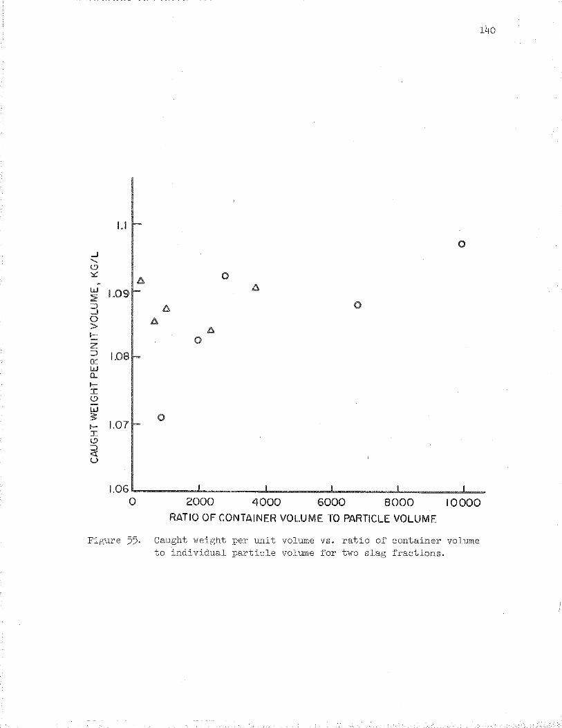
140
1.1
0 _J
' L? :>:
t:. 0 " w 1.09 2
::> t:. 0 _J
0 t:. > t:. f-
0 z ::J 1.08 0:: w Q_
f-I L? w s: 0 f- 1.07 I L? ::> <( u
1.06 L.....,. ___ ..,~_ ___ ....J.... ___ -~.. ___ ......~. ___ --!1......-
0 2000 4000 6000 8000 10000 RATIO OF CONTAINER VOLUME TO PARTICLE VOLUME
Figure 55. Caught weight per unit volume vs. ratio of container volume to individual particle volume for tw·o slag fractions.
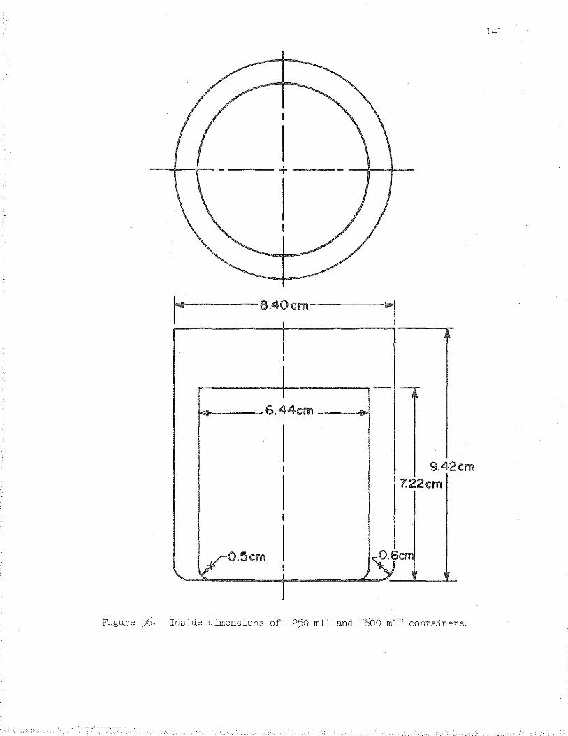
141
""~~~~------- 8.40 cm,-----li'>l~~
I
I
- -
6.44cm
I 9.42 em 7.22cm
I
' vo.Scm
: )~en I
Figure 56. Inside dimensions of "250 m1" and "600 m1" containers.

APPENDICES
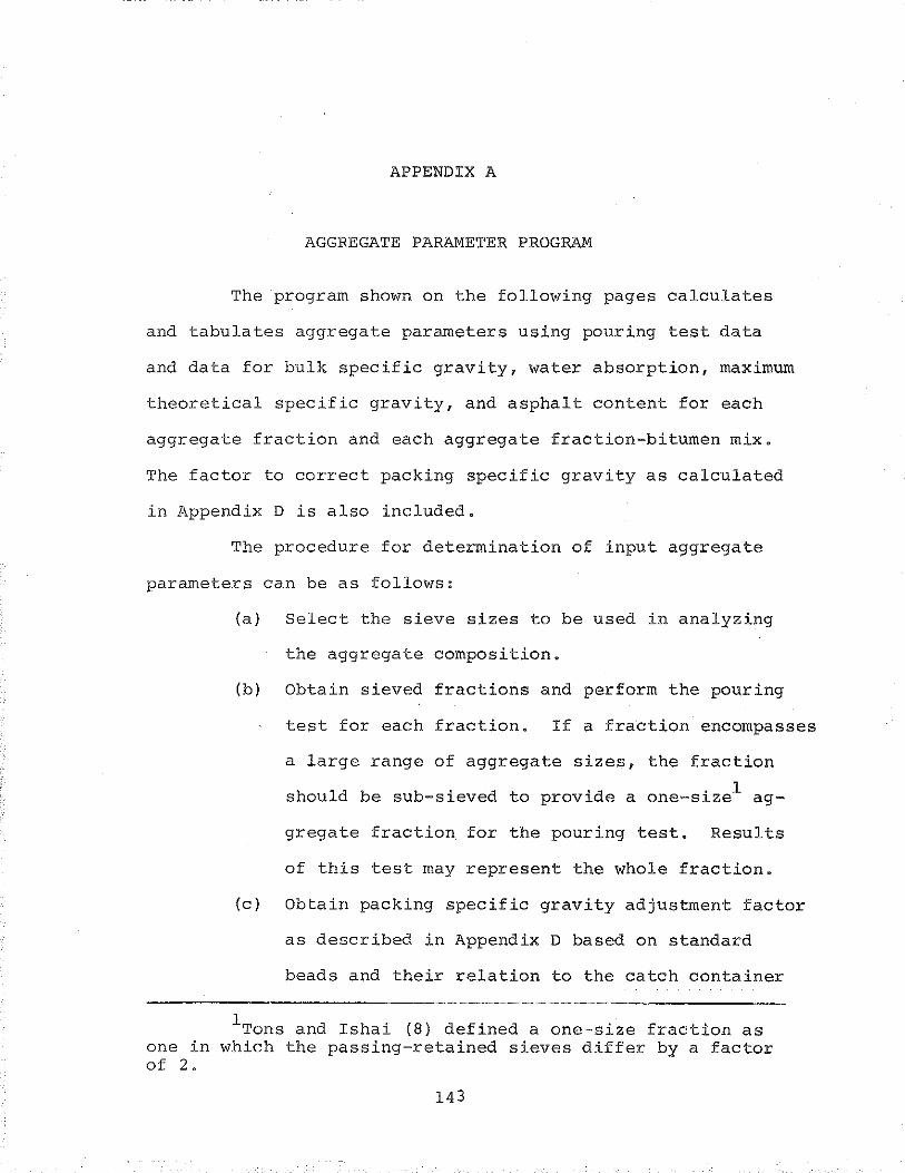
APPENDIX A
AGGREGATE PARAMETER PROGRAM
The program shown on the following pages calculates
and tabulates aggregate parameters using pouring test data
and data for bulk specific gravity, water absorption, maximum
theoretical specific gravity, and asphalt content for each
aggregate fraction and each aggregate fraction-bitumen mix.
The factor to correct packing specific gravity as calculated
in Appendix D is also included.
The procedure for determination of input aggregate
parameters can be as follows:
(a) Select the sieve sizes to be used in analyzing
the aggregate composition.
(b) Obtain sieved fractions and perform the pouring
test for each fraction. If a fraction encompasses
a large range of aggregate sizes, the fraction
should be sub-sieved to provide a one-size1 ag-
gregate fraction for the pouring test. Results
of this test may represent the whole fraction.
(c) Obtain packing specific gravity adjustment factor
as described in Appendix D based on standard
beads and their relation to the catch container
1Tons and Ishai (8) defined a one-size fraction as one in which the passing-retained sieves differ by a factor of 2.
143
144
employed.
(d) Obtain bulk specific gravity and water absorption
values for each fraction.
(e) Produce an aggregate-bitumen mix for each fraction.
Calculate its theoretical maximum specific gravity
and associated asphalt content.
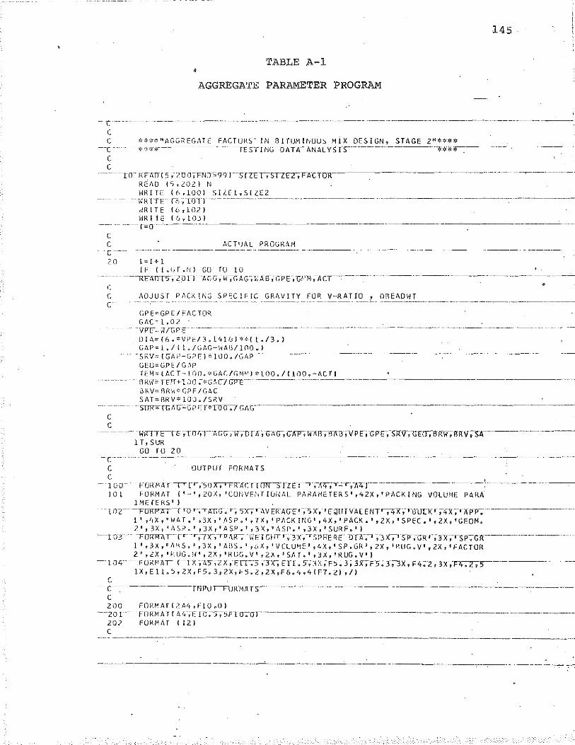
145
TABLE A-1 ' AGGREGATE PARAMETER PROGRAM
- r: -----------------·------------------------- ---------- -------------- ---
c c
--c-c c
****"AGGREGATE FACTORS' IN BITUMINOUS MIX DESIGN, STAGE 2''**** - --;:,~,,~,*-·-- ----------- -··---IESTI NG-DATA'- ANALv-STS _________ ---··--------···-***~----------.-- ---------·
- IO RFAD'f5, 2DO>ENJ"991--SfZFT-;-STZFZ>FATTUR----REJ\0 {5,2.02.) N WRITE: {6,100) S[LEl,SIZE2 \.;'RTTF. r.s -;TOl.T ··-··- ··---------- ------~- ----------------- .. -------------------------------
..-.IR IT E { 6 , l 02) r/R I T E ( 6 'I 1 i)J l
- ---I"[J ____ - -----------------------
c c c
ACTU1\L PROGRAM
20 l-=I+l IF I I.<;f .!·II
---I<FADT5;Zon GO TO 10 '. A"GG~-w-,-GAG-;hAtr;GPE1-GV:\\;7~.cr·---· ------------------------------------------
(
c C'
c c
"(
c c 100 10 l
ADJUST PACKING SP~CIFfC GRAVITY FOR V-RATIO ! DBEADWT
GPE=GPE/FACTOR GAC= l.O<' VPE= il/GPE------·------- -------·- ·- --------·---- ------ ------------- ----·--------·· -----·--
0 I A= { 6 ~ * V PC I 3 ~ 1 '+ l 6 l * '~ { l o I 3 ~ ) GAP=l~/(1./GAG-WAB/100.)
-SKV=' { GA P-Gtl E)* lUo-;-rG.6P .. GEO=GPE/G,\P fEM=(ACT-l00.¥GA~/GMkll*t00./(lOO~-ACT)
-· f3R\f:O:T"P1+1JC ;;->:•G!\C/QrE·~----~-~-·-- -·------ --~-------------------
l3 !<, V"" BR'.~"" GPI:/GAC SAT=BRV*lOO./SRV
- SUJ<=[C;AG"~GP E I"*T00-;-7 GAG---------·
WinTE-r-c. -PLD-4T--JI GG",li"1D rti. ~ 'G7\ G;'GA?f\TA!1;"!-r.lf3··;· V P E; -G p-~-SR"V,~ffRW;S!n.r;--s-;.----1 T, SUR
GO TO 20
OUTPlJT FORMATS
·- FDR74AT----rrr'--,-stT~"Fi=rACTT~-rzr:"'l-~-,"izt;·r--=Ti-A4--r-·----_--------------:-----------------
FORI"1AT ('-'rZOX,'COI'JVEt-~TIOi~AL PARM•IETER.S 1 , 1-tZX,'PACKING VOLUNE PARA [,~ErERS' I
-l o-z-- -FORf.f1.iT~\ 'D r9--,-AG'G-~ r; 5'XI'-J.\V ER-AG-E''-;3 x-,-t CQTII VAl ENT~X'~--1Wll[Kt- ;-!txt·• ll,p·p-~------------1 I , 'tX ' • w A T .. I t 3X , I Asp ~ I , 7 X f I pACK IN G I , 4X' ' PACK b ' , 2 X , ' spEC ~ i f 2 X, f GEOM .. 2°,3X 1
1 ASP.' ,3Xr'ASP. 1 r3X,vASP .. 1 ,3X 11 $URFo 1 )
--1UT ... --T-OR1'f!'l. ~-~-,------..-;-7AiTf11\'K"; -~~;r:I GHT ,-; 3X,~TSPRE At· D'fA~o-1 ·;-3X"r'_S __ P_ ~-~~ ,. ;--3y~-~--sp-;c·R--·-- ----------1' t3X,'fl 1iS .. ' ,3x,~ABS~' ,tiX, 1 VCLU~E' ,4x~•sP.GR' ,2x, 'RUG~V',2X, 'FACTOR 2', zx, •HJG~ \-1'' 2X, 1 R.UG. vI' LX, I SAT. 1 dX, 'RUG. V')
--104 -------FOiUfAT-- r-rx f'AYJZ A1Err-e-5 ~·3-XJ ETI ~-5-,- 3X ;·Fs-~- 3, 3X:.;Fs-;-J;-JXJF4---.;'2JJ>C,"F4~5----------·------~ l X t E ll .. 5 , 2 X, F 5. 3 _, 2 X r F- 5. 2 , 2 X, F 6 Q 4 , 4 ( F 7. 2) , I)
c ---c--:--- ---------rNPUT""FURHJITS' ___________ --------~--- ------------·-----' C 200
--2o 1 --zoz c
FORMAT(2A4,FlO.O) -FORMAT{A4.j:TID-;;-T;-SFTO:-ar·-~-------·---------··--------~-·----------·---------
FORMAT ( 121
-------- ------~-
---------·---
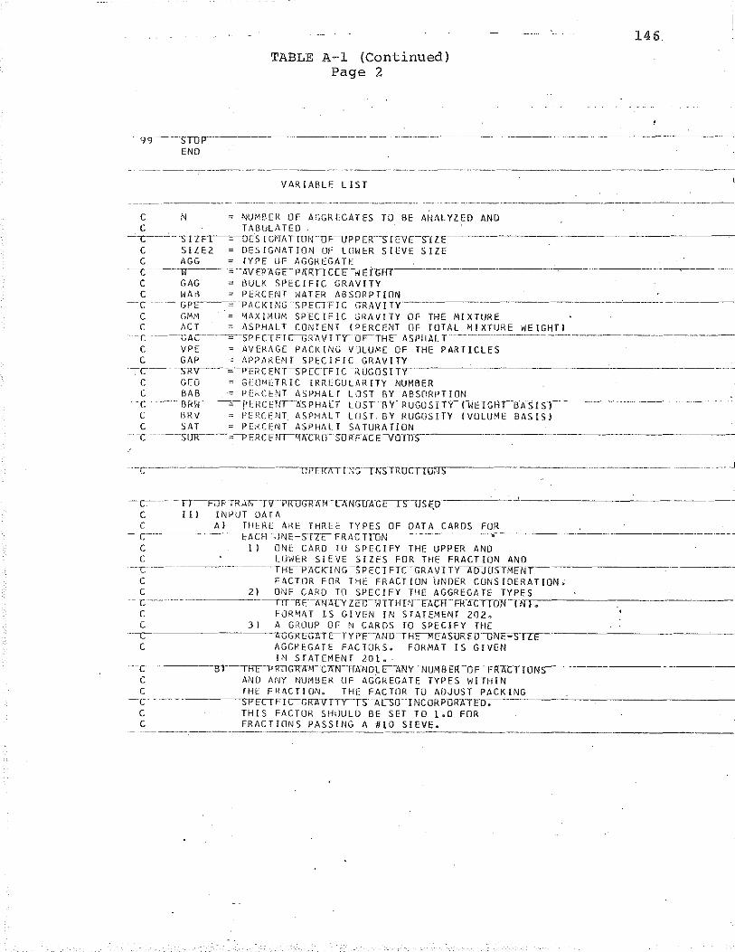
TABLE A-1 (Continued) Page 2
· 99 ----srur---_ ---------------------------END
VARIABLE LIST
C N • NUMBER OF AGGREGATES TO BE ANALYZED AND C TABULATED
146.
----c----··..:. __ S I 7 FT-----=-----nE S f G~l A TTTIN-·D F--u P P ER ___ S IE\1 E~SI lF -~----------------------------------
( SIZE2 DESIGNATION OF LOWER SIEVE SIZE C AGG TYPE Of AGGREGATE
--c-----1'1--- -WEFAGE- PI\RTTCEE -WETGRT----------------. ---C GAG BULK SPECIFIC GRAVITY C WA• PERCENT WATER ABSORPTION
--c GPE--~-.= -PACKING "SPECTFfC GRAVITY··----·-·-----··------·------------------------------
C GMt>l 1-111XP1UM SP-ECIFIC Gl~AVITY OF THE MIXTURE C ACT ASPHALT CONTENT !PERCENT OF TOTAL MIXTURE WEIGHT!
-c ----GAc------=--SPFCTFlcGRAVlTT OcTHE- ASPfiAl T -------------------------------------
( VPE = AVERAGE PACKING VDLU~E OF THE PARTICLES C GAP • APPAKENf SPECIFIC GRAVITY
--:-c--- -,Rv----··=-PERCENT:>PECTFIC RUGOSTT\'------------7 --------------------------
C GF::O = GE(JI.iETR IC IRREGULARITY NUMAER C BAB • PE~CENT ASPHALT LOST BY ABSORPTION
--.:-------- - BRw·------,- f'ERCENT-ASN!HT cosr·B y- RUGOSI TT n-IE[(;RT--B-Asrs-r------------------------C BRV • PERCENT ASPHALT LOST. BY RUGOSITY !VOLUME BASIS} C SAT • PERCENT ASPHALT SATURATION
-- T ------sUR-----=-I'ERCF~flATRO- SORFATE--vo-rn-:;--
----~--- , ... ----~-------- ------------ . . J
- c---- - n-F<JF TR-1r.-rv--PK1JGJUiWCANGTFAGrT:>-USE.O ________ _
C Ill INPUT DATA C A) THERE Al<E THREE TYPES OF DATA CARDS FOR - c- -----------ElicH fJl'TE~srrc--FR<rc rroN ____________ --,-------------------c I l ONE CARD TO SPECIFY THE UPPER AND C LOWER SIEVE SIZES FOR THE FRACTION AND
---c ---------···-- ----THcl'MXfNG -!:PEC !FTCGRAVJ Tr,>rnOSTMFl-ir
C FACTOR FOR THE FRACTION UNDER CONSIDERATION. C 2} ONE CARD TO SPECIFY ,THE AGGREGATE TYPES
-- c-- ------------nr-roF-A"fi\1.Y ZED-WTTffHrTACR-·FiftiCTTON-lff;_.----
C EOR~AT LS GIVEN IN STATEMENT 202. C 31 A GROUP OF N CARDS TO SPECIFY THE
-·--c------------·AGGREGJ\TcTYPF-AIW-THET-IFA-SUP:EO.<JNF'o;TTo ________ _
C AGGREGATE FACTORS. FORMAT IS GIVEN IN STATEMENT 201.-
--c- --------rn--THF-1' RTIGRAM-CAW-HA1JO[ c-ANYNUM 8 ER --oF-FRI\CnOfl> C AND ANY NUMBER OF AGGREGATE TYPES WITHIN C THE FRICTION, THE FACTOR TO ADJUST PACKING
--c ---------sPECTFJc-G!<AVTTTTS. ACSO -INCORPOR-ATEIJ-. -----C THIS FACTOR SHOULD BE SET TO 1.0 FOR C FRACTIONS PASSING A #10 SIEVE.
APPENDIX B
COMPUTER PROGRAM FOR MIXTURE DESIGN TABLES
The program shown on the following pages use6 input
from aggregate analysis and from the aggregate parameter
program to construct design tables for prediction of optimum
asphalt content. Procedure for use of the design tables is
outlined in Appendix E.
147
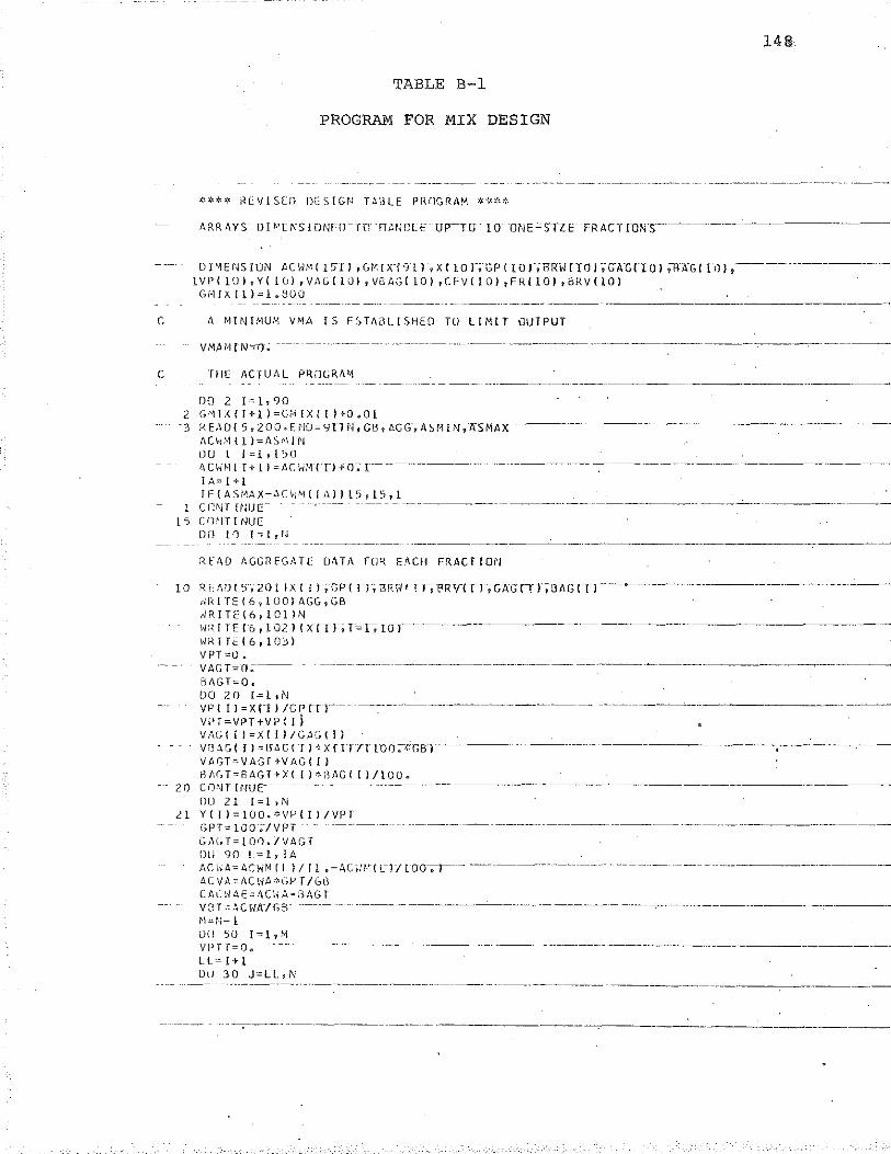
148
TABLE B-l
PROGRAM FOR MIX DESIGN
>:•***' R.tVISE/1 n;:siGfJ TA'JLE PROGRAM****
D I-'-lE i~S llJN ACHr-n-15IrJ-G/':rX·r 9-t Y1XTTO r;·-cPTTOTiBRW £TO J t-GAG{T0Ti1rA-GITOl"f ~---------~~--~ 1 V P ( 1 0 ) , Y ( 1 (J) tV;\(.( l;}) , VB AG ( 1 0 ) , C F V ( t 0) , F R ( 1 0) , 6R V ( l 0) Gf.IIXIll=l.800
- -~ -- ------------- --~-- --- -----~--~~~-----~~~~-----
C A MINIMUM VMA IS ESThaLISHEO Ttl LIMIT OUTPUT
C fi-lE ACTUAL PR!JGRA"''
DO 2 I=l,90 2 G '\I X C I+ 1 ) -= Gi'.-1 I X I I l tO ~ 0 1
-3 R E:\0{ 5 i200, E i'J0='9llN?GB ,--AcG·;-trsmr;r-;1\SM'AA- ------·-----~------···--~~~ An;,\1 ( 1 )=AS;\\ IN DO l I:::ld50 ll.CWI-1( T+ll ;:;1\CW:HT) -f-0~ r-- -----~-----. -·---------,.-------~------~-----------~--~--------~-
IA=I+l I F { A S,'-JA X-.'. C f.' M { I A ) ) 15 , 15 , 1
1 CCr-.JT H:UC - ----- ------~~~--~----- ---------------------------~------~--
15 Cn~!TINUC DD 10 I=l,N
---~---------~-~~--~--~------~~- ~~~----~~--
RfAD AGGREGATE DATA FUR EACH FRACTION
10 R El\Df s-·,· 201 IXTf l-j. Gfr(TTi1JRff/'!Tf)FRVTTTt1:;-AG{!1-;lJ.tYGTtl- ---o----------~~-~~----~RITE(6?lOOlAGG7GB ,.JRITI:::(6,10l)N WRI TEC6, 102 J fXTI r; T'o=T9IOT WR [ TE ( 6, 10.::.>)
VPT=O" Vl\GT=o;;---~-
BAGT-=0. DO 20 I-=1 ,N
------------~-------~---------~-~ ---~------- -~-
vP I II= X c-1 I /G P rrr--- -~-- -----~------~---~-- ------------VPT~VPT+VP!Il VAG{!)=X!Il/GAG!II VBAG( Il=frAG{ I l*X[!TilTOO~<'GBT~~~~ ---~~------- --~---~~-VAGT=VAGT+VAG([) 8/\GT=BAGT+X( I )>:<afiG( [ )/100,.
20 CO~H H-IVE___ ·-··------ ------~~~-
00 z 1 r = 1 , N ll Y(l)=lOO.~VP(Il/VPT
---- -------
GPT= 100 ;/VPT ------·~-- ------ -------~-------~ ---------------~------~--------·-·----~--~-~--
G/\l;T=lOO./VAGT DU 90 l=l,IA f1C hA-= ACWM ( L} If l .-AUU.ff LT/ roo·--;;-y----- ------· -~---------- -----------------. ··------------------------- ---------~-------------ACVA=ACWA*GPT/G8 CACWAE=ACW~-RAGT V 8 T = ~ C WA"/ G g- ------------- ------ ··-----~---- ------------~------ -- ~------·------- -·-------:-----·----------·----------------
1'1-= r-i-1 D!l 50 I=l,M VPTT=O .. -. --LL=:ol+l Utl 30 J=LL,N
-~---------~·~-----c-
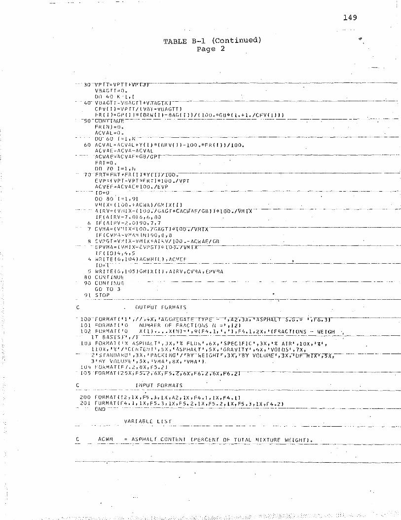
c
c
c
TABLE B-1 (Continued) Page 2
30 VP fT=VPTHVPT;rr·----~------~---
VRAGTT=O~
on 40 K==t,r
149
40- VBAGTT .:::VBAGTT +Vffi'\-GTK_J ______ ~------- ·----·--------·-----------------~- -------------------~----
CFVIII=VPTT/IVBT-V8AGTT) F R I I l = GP I I ) * I BR WI I ) - 8 AG I I ) ) I I 100. *G e *I l• +l· /C F VI I l ) l
-50 -CDNTT NliE -·-- - ------- -- -·------------------ ------------------------------------------·------
FRIN)=O. ACVAL=O. oo- 60 I =I, N ----------------------------------
60 ACVALo::ACVt,L+Y(l)*{BRV{ll-lOO.*FR(ll)/100., ACVA!:~ACVA-ACVAL
ACWAE~~CVAEOGB/GPT
F R T =0. DO 70 I==ld\1
70- FRT~FRT+FR{T l*YfTJFroo.-· EVP=(VPT-VPT*FRTl*lOO./VPT ACVEF=ACVAE*100./EVP .
- I 0=0- - - -------·
DO 80 1=1991 V M I X= ( 100 .. +A_ C HA l /G.~1 1 X { I )
------------------
h. IR Vc= ( Vi·II X-( 100-~-/GAGT+CAGf/YFlGH rl *1-0U----:--/Vl.ffX ----------------- -·-------------IF(AIRV-7.0)6,6,80
6 IF(AIRV-2G0)90,7?7 7 CV!1A" IV'Il x-·100. /GAGTWIOO-;-TVATX--------------
IF(CV•'}•\-VMt,'-i !N)gQ,8?8 8 EVPGT=V~[X-VMIX*AI~VIlOO~-ACWAEIGB
- EPVMA={ VMfX:...;EVPGTr>:' roG· .. 7VHTX _:_::_ __ IF( IOJ4,ttt5
'' WRITE(6,lll4)ACWNfi.J,AC:11EF ID"l -- ----- --- ------ ------- ------ -------- -----
WRITE(61l05)GMlX(IJ9AIRV,CV~A,EPV~A 5 80 90
CO~T !NUE C ONT f !'-JU C --- -------------------- --------------------GO TO 3
91 STOP
OUTPUT FURHATS
100- FORMAT ( '1' ,-/I 1-+X, r-A"G-GKE"GATE"-TYP-F :....----r ;-·~-,~Xf11A-SPHlllT--s-~·c;:: ,-,~1,------
101 FOR•\1t..T( '0 NUI-YIRER OF FRf,CTirJ•'~S ii =' ,12) 102 FUk!'1AT('O X(l),~~aX(~JJ= 1 ,9(F4 .. 1, 1 , 1 ),F4Gl,;!!Xr 1 CFRACTIONS- WEIGH ,
1 T BASIS l"', n- -------- ---------- --- ---- ---- ----------------------------·--103 FORMAT('% ASPHALT',3X,'% FL0\·:',6X, 1 SPECIF1C',3X, 1 % AfR 1 ,lOX, 1 %',
11 ox ~ '% • 1 'c C:N r en ' , s x , 1 ASP HAL r ' , s x , ' G RA v IT v ' , ,_,.x , ' vo 1 o.s' , 1 x , 2 1 STANOA RD' ,3X-; 1 PACKrNG~7i"RT.WE IGHT r--;-3 )C,- 1 'BY-·VoUmEr,"3X·;---.oF--MTx-r;-5"X"~--~---·-----·-----
31HY VfllU,'1 f 11 5X 1
1 Vi"lA 11 8X, 'VMA 1 ).
104 FOkMATIF7.2,8X,F5~21 l 0 5 FOR1•rAT 1·2 5X, F 5-;.-z ,--6X-IF5:ZI-5XVF6_o_Z?6X-;F6-~-zr----·-·-------·-. --·-----------·----··--------
INPUT FORMATS
2 0 0 F 0 f< MAT ( f 2 , 1 X , F5 .. J v l X , A 2 r lX , F 4 ~ 1 , l X r F 4 o Ll 201 FUR/~AT{F4.1, lXvF5o3, lX,FS. 2,1X,F5~2,1X,F5~3,1XrF4 .. 2)
END --- --------------- ------- -----------------------------------~-- ------
VARIABLE LIST
ACWM ASPHALT CONTENT IPENCENT OF TOTAL MIXTURE WEIGHT). -- ·----- ----·- ·-----------· -----------·----~---· -------- ----~----- ~------ ~------------··------
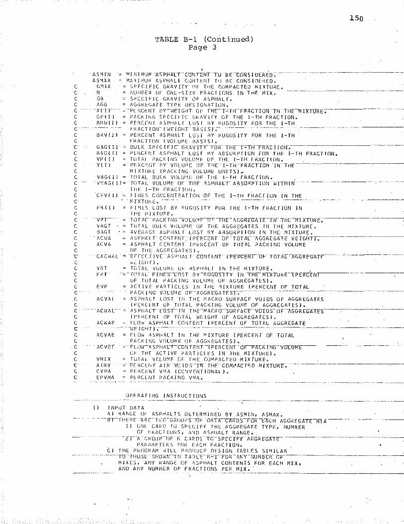
c c c c c c c -c--c c c c c c c c c c c c c c c c c c c c c c c c c c cc c c c c c c c c c c c -c c
TABLE B-1 (Continued) Page 3
150
ASIHN -~ MJN!'IUM A>Pf'AlTTIJNHNT ni BE-1:0NS!O£REO; ----A$~'>1AX
G't [X N GB f,GG XI! r· GP I I I Bln-1 (I)
BRV ( l l
GAG'(Tl B<\G I t I VP (II Yl I l
VAGI I l
= MlXIMUN ASPHALT C~NTftJT TU BC CUNSIOEREO. SPECIFIC GkAVITY OF THE: CUMPACTEU MlXTllRE .. ~UMBER ()F ONE-SIZE FRACTIONS TN-THE-MfX~
SPECIFIC GRAVITY OF ASPHALTo AGGREGATE TYPE OfSIGNATIUNo
-pE RCENr tlY-,Fl GfH OF THE- FTH. FRACTION TN THE-1~ l~T\JRE:.--·------------- -~~-PACKING SPECIF[C GkAV1TY OF THE I-TH FRACTION. PERCfr"H /ISPHt\Lf UJ.Sr RY RUGOSITY fOR THE I-HI -fRACTfOW-(~1E[GHT :lASfSr .. --- --~----
PEf{CENT ASPHALT LO~T RY RUGOSITY FOR THE 1-TH FRACTifiN (VOLUME BASISID BULK SPECIFIC .GKAV1TY ___ FOR- THF_T_.-:-n-f-TR7;;.Cl J"C;'N_e ____________________ ~~-- -----~-
P~I~CE~lf ASPHALT LOST HY ABSORPTION fOR TtlE I-TH FRACT[ON6 TtJT/d_ PACK Ii'J~ VULUNE OF THE I-TH FKACT£ON~ PF.HCEfiT f'·Y VOLUME TJF THE·l..:_TH·--FR.lfCTfON -nf-THE-----------~--f.IIXTUkE (P/ICKING VULU1\JE UNITS)~· TOTAL BULK VOLLrH=: OF THE l-TH fRI\CTWNo
VB AG ( I l =--TOTAL ·vat UME ___ OF' THE --n:SPHAlT' J\BSORPTI orr· W ITHiw------.-·-----
CFVI I l
FR (I I
vPr-VAGT !31\GT
-ACYJA /l.CV/•
---- CA-CHAE
VB T FRT
EVP
TH!-: l-Hl FRACT I(I,\J. FINES CU~CENTPATION OF THE I-TH FRACTION IN THE ,'-; rXTUR"E ~-- ------ ----- ---------- ---
fl'fES LOST BY PUGDS!TY FUR THE 1-TH FRACfiON IN T/--IE n!XHJRE. TOTAc P1\CK !NG ·vrJLUHtU"--rFlE-AGGKEGATE-Trr THLi-HXHI~IO; ~------ -----~
Tf.JT/IL BULK VDLU'lE Of ThE AGGK.EGATES IN THE NIXTURE. AVERAGE A~l1 i~AL-r LOST BY AdSO~~TION IN T~IE MIXTUREo ASPHli"L T CCNTEI'lT. ( PFRCENT- DF--TOT Al--AGGREGA'TE WEIGRTr .. ---~- -·----·---- ----ASPHll.LT C:CNTF.NT (PERCENT OF TOTAL PACKING VOLUME UF TH~ AGGREGATESio EFFECT TVE . ASPHALTCONIT~ITTPERT.ENTIJFIOIA[-·-JI'GFRH;-ATF- -------'--~~-1-.ElGrlr)a
~ TC1TAL VGLUME UF ASPHALT IN THE MIXTURE. , - fC'TAL F!NESTOST DrRUGDS1TY !N THE-IOTXTURE-lPERCEN.----~
~F TUTAL PACKING VOLUME OF AGGREGATES)o ACTIVE !-'fdHICLES IN THE NIXTURE (PERCENT OF T.OTAL P 1\ CK I i\JG"' VCJ CUT~ e· 0 F- f. GG KEG,\ T E s-r~------- ~ ~---.·--~-------. -~-------------------
ASPH~LT LOST lti Tf1E M~CRO SURFACE VOIDS OF AGGREGATES !PERCENT UF TUTAL PGC~ING VOLUME OF AGGREGATES).
--- ACHAl-- ASPHALTTOST!i-J THE-~<\CRuSURFACEVUIOS-OFI\G-GREc-ATt!>--.-----------~--
ACWAE
ACVAE
il.C VFF
VNIX A IRVCVMA EPVMA
fPERCENT OF TGT~L WEIGHT OF AGGREGATESio FLOW ASPHALT CO~TE~iT (PERCENT OF TOTAL AGGREGAT~
-\-,'E [ GHTT.--·-------------··-·-~-------·---------~----'---
fLOW ASPf4ALT lN THE MIXTURE (PERCENT OF TOTAL PACJ<ING VfJLU!.\E DF- 1\GGkEGATES) ..
- FliJW-1\ SPHAL"T-CCNTFl"lT --(PERCENT' -or-PACK I NG--VG[UMF·------~------·-~·----'-CF THE ACTIVE PARTICl.ES IN THE MIXTURE}. TUTAL VCLU.'1E OF THE CfJI"~PACTF.O 1'-1lXTURE.
- PE RCE~i T A IR---vt:ro S ·rw THE. COM~ ACT'OIJ M l XTURF-. --- ·--- --PERCENT VMA (CC~VENTIONAL}. PERCENT PACKING VMA.
OPERATING INSTRUCTIONS . ------- ------~-·----· --.-----~~-----~------ ·-·------------------ --·~-----·- ----
l) lNP0T OAT1\ 1\) :.{ANGE OF ASPHIILTS UETER:'HNEO BY ASM(N9 AS/1AX,
- -·-aT-TI-lE Fl [ ARE-- H,' r~---GKClliP S --DF" fJ/\TA--C"IIKD'S-FOR-tA'C H-AGGR EG-ATI-Ml )(---~-------~-- --~ ll UNE CAkO TO SPECIFY THE AGGI--l.EGATf: TYPE, NUMBER
OF FRACTIONS~ A~D ~SP~lALT ~ANGE,. - -- ---- 11· A -GHOUP-nF-·;r C oRDS-TO.SPECTFY-7rGl;RFGATr----~-------- ----------~---·· --
PARI\METERS FfJP. EACH FRACTION-.. C) THE PkOGRAM ~ILL PROfliJC~ DESIGN TABLES SIMILAR
---·------TO -THOSE 5HO"?li'r.Tt~- T A3LF--B:...-r--FOR -Ar\Y-NUHB'ER- ·c-F·~~---~~---~---------MIXES, ANY KANGE OF 4SPHALT CONTENTS FOR EACH MIX~ AND ANY NUMBER OF FRACTIONS PER MIX •.
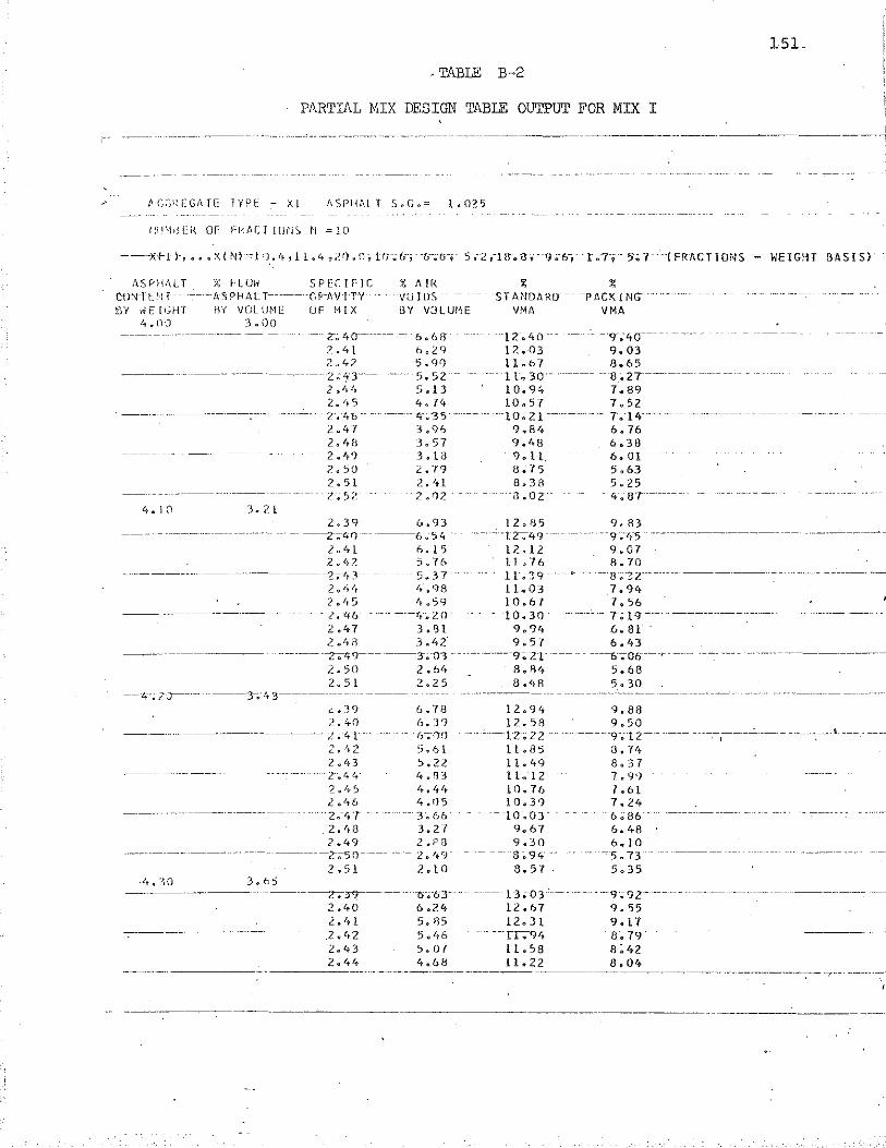
,--
lSL
-TABLE B-2
PARTIAL MIX DESIGN TABLE OUTPUT FOR MIX I
' -----------~---~--------- ----------·
fi.SPHI\LT % flOW SPE[IFIC Cii"t-T-E 1·1 T-- -----AS PH At T----- -cF-AV-Il'Y EY ~E[GHT HY VOLlJME OF M[X
4~!1J 3&00 z-~ 4o--Z.41 2a4?
------------------------------ L;<';t'3
%AIR % VU IDS ---- ST MIOARo- ---pACK !NG· BY VJLUHE VMA VMA
-1z.4o--12.03 ll .. b7
. 11.30
-9.-40--9.03 8.65
--8. 27-~-7.89 7. 52
? ~'· 4 2 ~ '• 5 2-. 'tO 2.47 2.48 2. 4ry-z.so 2&51
6. 68 b~29
5.Q0 ·5.52 5.13 4. 74
-4-.35
1 o. 94 10.57
--la;zl--9.84 9~48
'). 11.
. - T; 14 ____ - -- -------
4. l () 3. 2 1 -- L·.; 52
~L96
3.57 --3.13 L~79
2. 1-t 1 2.D2
2.39 6.93 ·---- --· -- ----z--;;--41/ -- -~-6.-?"
l.4L 6.15 2~42 5.7&
-------- ~.-~t J -- 5 .. 3 7 2.44 ~.9R 2o45 4.59
- z.46 -------t.--,zo 2.47 3.~1
2 • .'tR 3.42"
e .. 7s
12.B5 -·-rr.4o
12.12 11 • 7 6 1 t .. 39 11.03 10.67 10.30
6. 76 6.38 6.01 5.63 5o25
- 4" 8 y---·-----
9.83 ~-- ""9'~''{t'5
9.07 8. 70
-a.;;-3z----- ----------------
7.94 7 9 56
- 7; 19- - ~---- ---- ------ -
6.81 6.43
--- ---------- .. ------ -;>-;-49 ___ ----3; 01
9.,94 9.57
------- 9; Z1 - ----6-706-- c.-- .
2.50 2.6lt 2.51 ,2 .. 25
---4--~ zo---·-.. ----J-.·43------------ -------
Lo39 2.40
. -------- ---------- 2. 41•
2. l-t3 .. z·.t-tt.-
2 .t+ ~
2. 0 1t6
z. 1t8 2.49
-------,-,-5o··
''t.:-\0 3~6S
6.78 6.J'} 6-;-rHJ
5.61 5.22 4;83 4. 4 1t
4.05 --- 3.66""
3.27
2.10
8.B4 8 .. 48
12~9't 12.58
--- -1z; 22 ·· 11.85 11.49
- 11.·1z 10.76 10.39
- 1o.or 9 .. 67 9.30 3;.94 8o57
5.,68 5.30
9.88 9 .. 50 9-.-1z---
n. 7't 8.3 7 7.9') 7.61 7. 24 6. 86 -6.48 6.10
-5.73 5 .. 35
----------------- --------' ---- -----
-------~---------------z-;-,-<r-~---o·.-63' 13;03.- --q;n----- ---~ ---------- -----------2~1+0 6 .. 24 12 .. 67 9~'55
2.41 5.85 12.31 9.!7 -------~- ·-------;z-;;--tt.-z-·----- --s-~-z,.o ---·- ---rr..-94---------------s-;7r--------· ----- -------------
2.43 5.o7 11.ss a:4z
~---=z_:__. 4 4 ----~--4_. 6_8__ ---~-l_l._z_z ______ a_._o4 __________ ------------~ -~--- ____ _
APPENDIX C
POURING TEST AND PROPOSED STANDARD APPARATUS
The pouring test is used to directly measure the
packing specific gravity of an aggregate fraction. This test
was developed by Tons and Ishai (8) for six one-size fractions.
The basic pouring test assembly is shown in Figure C-1, and
the two stages of modification prior to the present proposed
standard apparatus are detailed in Table C-1. Table C-1 also
presents the proposed standard apparatus based on current
knowledge of the pouring test. The following should be noted
in connec·tion with the proposed apparatus:
(a) A conical bin is used for all aggregate sizes.
This is accepable because aggregate head within
the aggregate holding bin was found to be in-
significant in determining packing. efficiency of
the caught sample.
(b) Orifice diameter is variable to allow selection
of an orifice for each fraction and each aggre-
gate type within the fraction for greatest test
efficiency.
(c) A fraction range, rather than a specific fraction,
is specified for each container assembly. The
entire range of aggregate size likely to be
encountered in bituminous mix design is considered,
MICHIGAN DEPARTMENT OF 152 TRANSPORTATION LIBRARY
LANSING 48909
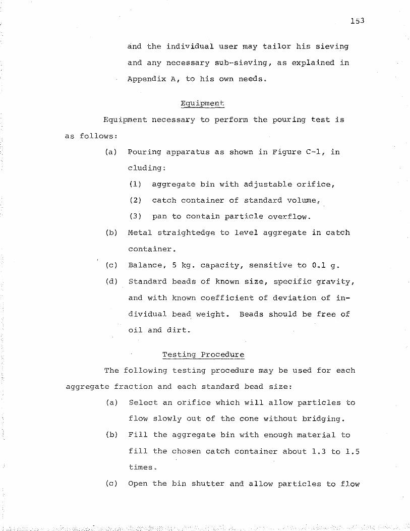
and the individual user may tailor his sieving
and any necessary sub-sieving, as explained in
Appendix A, to his own needs.
Equipment
Equipment necessary to perform the pouring test is
as follows:
(a) Pouring apparatus as shown in Figure C-1, in
eluding:
(1) aggregate bin with adjustable orifice,
(2) catch container of standard volume,
(3) pan to contain particle overflow.
(b) Metal s·traightedge to level aggregate in catch
container.
153
(c) Balance, 5 kg. capacity, sensitive to 0.1 g.
(d) Standard beads of known size, specific gravity,
and with known coefficient of deviation of in
dividual bead weight. Beads should be free of
oil and dirt.
Testing Procedure
The following testing procedure may be used for each
aggregate fraction and each standard bead size:
(a) Select an orifice which will allow particles to
flow slowly out of the cone without bridging.
(b) Fill the aggregate bin with enough material to
fill the chosen catch container about 1.3 to 1.5
times.
(c) Open the bin shutter and allow particles to flow
J.54
into the catch container.
(d) Carefully level particles to the top edge of the
container with the metal straightedge.
(e) Weigh the contents of the container and record
this as the test response.
(f) Repeat this procedure for as many replications
as desired.
(g) Repeat for as many different aggrega·te fracticms ·
as necessary.
Calculations
Calculation of packing specific gravity can be per~
formed as follows:
(a) Perform the desired number of replications of the
pouring test for standard smooth particles.
Average the test results. Divide the apparent
specific gravity of the beads by average caught
weight and obtain the packing specific gravity
factor, Q.
(b) Using the same container, perform the pouring
test for the aggregate fraction represented by
the standard beads. Average the test responses
for the replications performed and multiply this
average by the packing specific gravity factor
to obtain the packing specific gravity of the
test aggregate.
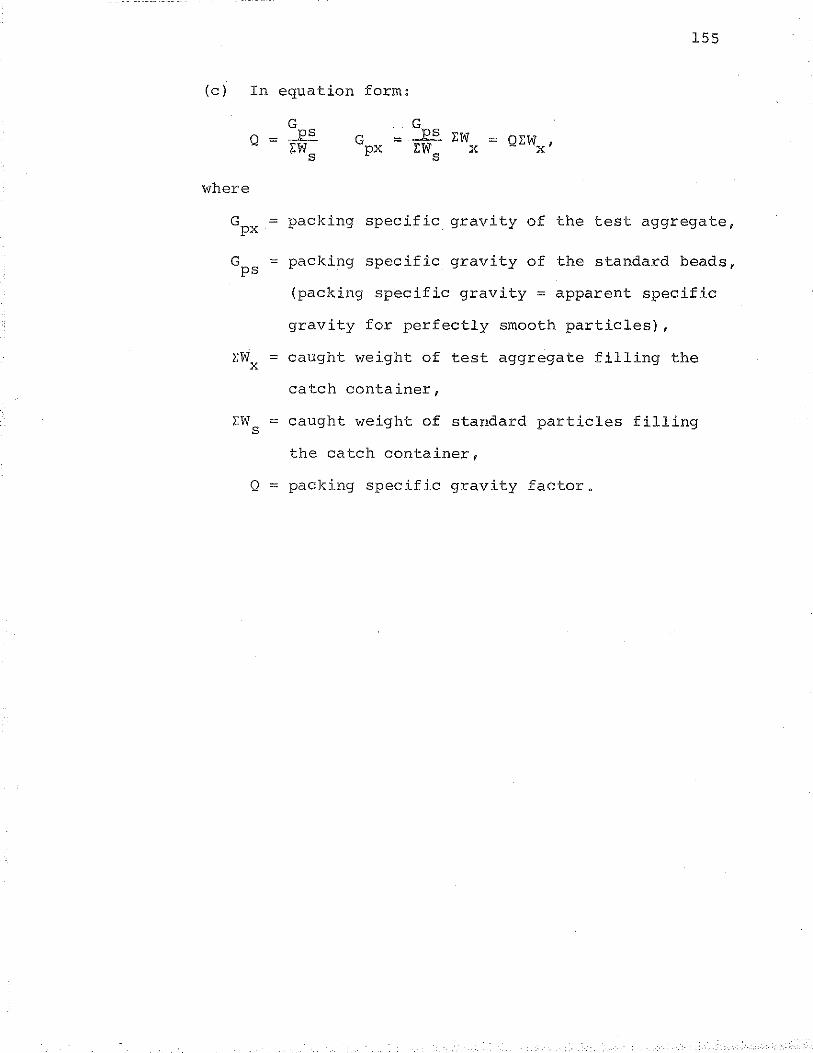
155
(c) In equation form:
G Gps Q = ~ G
_, EW = Ql:W , ~w px l:Ws X X s
where
Gpx = packing specific gravity of the test aggregate,
G = packing specific gravity of the standard beads, ps
(packing specific gravity = apparent specific
gravity for perfectly smooth particles),
l:Wx = caught weight of test aggregate filling the
catch container,
l:W = caught weight of standard particles filling s
the catch container,
Q = packing specific gravity factor.
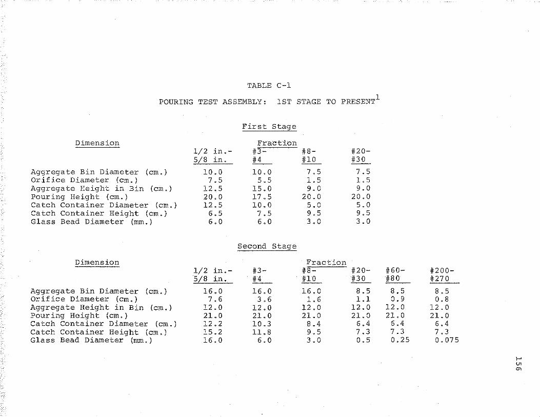
TABLE C-1
POURING TEST ASSEMBLY: 1ST STAGE TO PRESENT1
Dimension
Aggregate Bin Diameter (em.) Orifice Diameter (em.) Aggregate Height in Bin (em.) Pouring Height (em.) Catch Container Diameter (em.) Catch Container Height (em.) Glass Bead Diameter (mm.)
Dimension
Aggregate Bin Diameter (em.) Orifice Diameter (em.) Aggregate Height in Bin (em.) Pouring Height (em.) Catch Container Diameter (em.) Catch Container Height (em.) Glass Bead Diameter (mm.)
1/2 in.-5/8 in.
10.0 7.5
12.5 20.0 12.5
1/2 5/8
6.5 6.0
in.-in.
16.0 7.6
12.0 21.0 12.2 15.2 16.0
First Stage
Fraction #3-#4
10.0 5.5
15.0 17.5 10.0
7.5 6.0
Second
#3-
Stage
H_ 16.0 3.6
12.0 21.0 10.3 11.8
6.0
#8-#10
7.5 1.5 9.0
20.0 5.0 9.5 3.0
Fraction #8 #10
16.0 1.6
12.0 21.0 8.4 9.5 3.0
#20-#30
7.5 1.5 9.0
20.0 5.0 9.5 3.0
#20-#30
8.5 1.1
12.0 21.0 6.4 7.3 0.5
#60- #200-#8 0 #270
8,5 8.5 0.9 0.8
12.0 12.0 21.0 21.0
6.4 6.4 7.3 7.3 0.25 0. 07 5
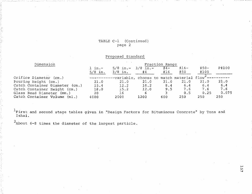
Dimension
Orifice Diameter (em.) Pouring Height (em.) Catch Container Diameter {em.) Catch Container Height (em.) Glass Bead Diameter {mm.) Catch Container Volume (ml.)
TABLE C-1 (Continued) page 2
Proposed Standard
Fraction Range l in.- 5/8 in.- 3/8 in .. - #4- U6-5/8 in. 3/8 in. #4 #16 #50
-----------variable, choose to match material 21.0 21.0 21.0 21.0 21.0 15.4 12.2 10.2 8.4 6.4 18.0 15.2 12.0 9.5 7.6 20 16 6 3 0.5
4000 2000 1200 600 250
#50- P#lOO #100
flow 2 ----------21.0 21.0
6.4 6.4 7.6 7.6 0.25 0.075
250 250
1First and second stage tables given in "Design Factors for Bituminous Concrete" by Tons and Ishai.
2About 6-8 times the diameter of the largest particle.
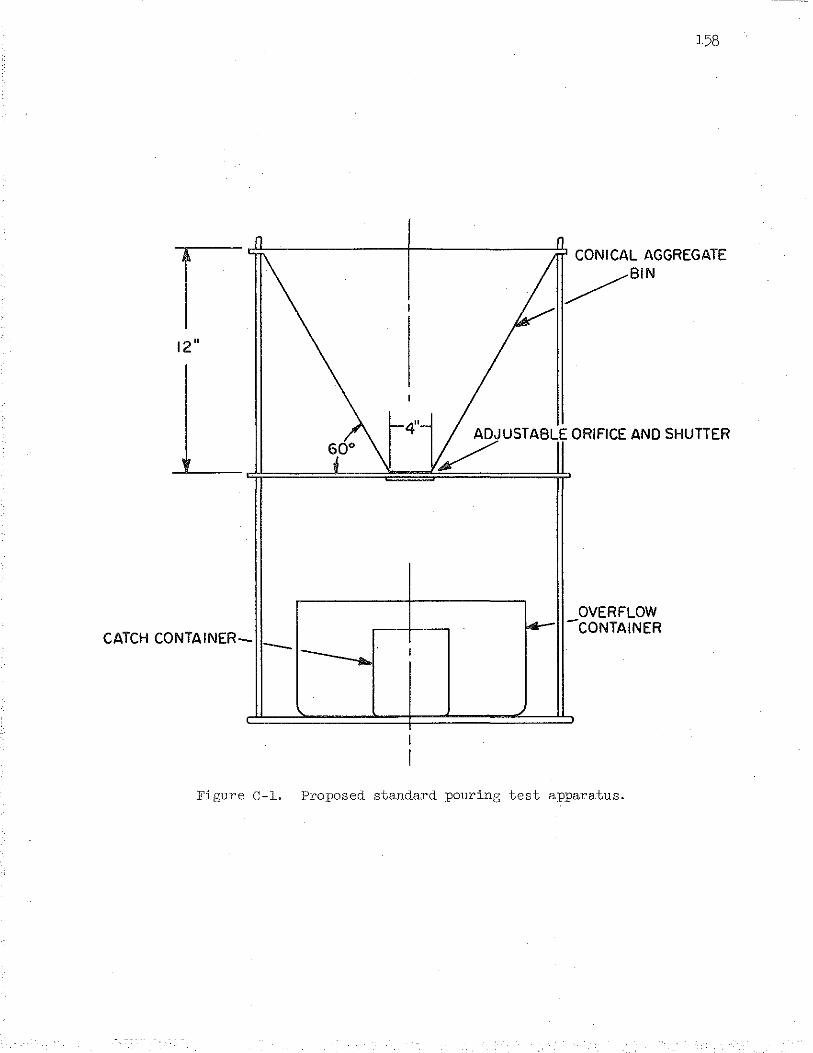
158
ADJUSTABLE ORIFICE AND SHUTTER v
CATCH CONTAINER-
OVERFLOW -CONTAINER
Figure C-l. Proposed standard pouring test apparatus.
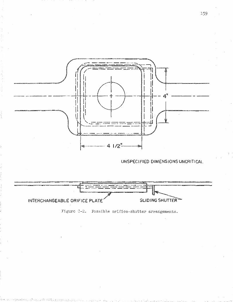
159
----
(;~----==--=--=----=--="'-. --------- =n / ------ 'I l I 11 I II
II :I --+-- t --+- -i>-l-1-TII-1 - 4' -
II II
li ll I 11
'-=-~===== :-::iJ --------- -'
1 ________ 1
~-41/2'~ UNSPECIFIED DIMENSIONS UNCRITICAL
INTERCHANGEABLE OR I!:::;----~s Figure C-2. Possible orifice-shutter arrangements.
APPENDIX D
CORRECTIONS TO PACKING SPECIFIC GRAVITY
The following factors were found to be significant in
determining porosity of the caugh·t sample in the pouring test:
(a) Pouring height.
(b) Pouring time.
(c) Ratio of container volume to individual bead
volume.
(d) Variability of bead size within a single nominal
bead size.
An additional factor was the ratio of container area
to container volume. It was not known whether or not this
factor was significant. This factor was included as a
variable and will be shown to be insignificant within the
range encountered.
The variables of pouring height and pouring time were
held constant by using the same pouring height for all tests
and by choosing an orifice size which would just preclude
bridging of beads in the cone.
A variety of bead types and sizes was employed to
provide a wide range of container-bead volume ratios, bead
variability values (defined as the coefficient of deviation
of bead weigh·t) , and container area-volume ratios. Table D-1
shows the containers and beads used. Note that three small
160
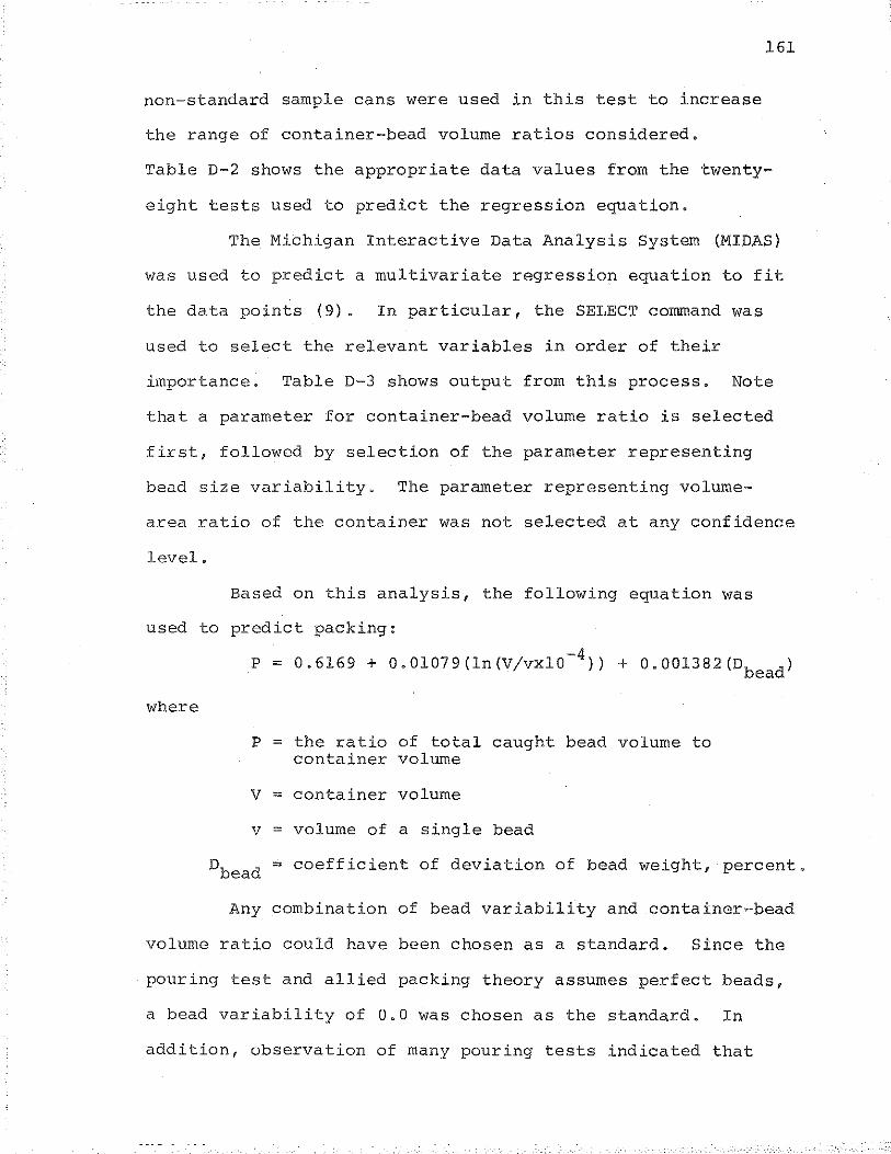
161
non-standard sample cans were used in this test to increase
the range of container-bead volume ratios considered.
Table D-2 shows the appropriate data values from the twenty-
eight tests used to predict the regression equation.
The Michigan Interactive Data Analysis System (MIDAS)
was used to predict a multivariate regression equation to fit
the data points (9). In particular, the SELECT command was
used to select the relevant variables in order of their
importance. Table D-3 shows output from this process. Note
that a parameter for container-bead volume ratio is selected
first, followed by selection of the parameter representing
bead size variability. The parameter representing volume-
area ratio of the container was not selected at any confidence
level.
Based on this analysis, the following equation was
used to predict packing:
p = 0.6169 + O.Ol079(ln(V/vxl0-4
)) + 0.001382(Dbead)
where
p = the ratio of total caught bead volume to container volume
v = container volume
v = volume of a single bead
Dbead ~ coefficient of deviation of bead weight, percent.
Any combination of bead variability and container-bead
volume ratio could have been chosen as a standard. Since the
pouring test and allied packing theory assumes perfect beads,
a bead variability of 0.0 was chosen as the standard. In
addition, observation of many pouring tests indicated that
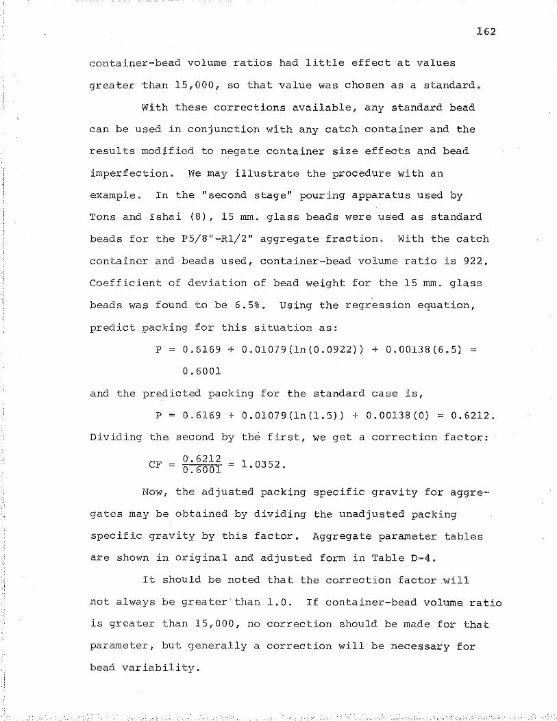
162
container-bead volume ratios had little effect at values
greater than 15,000, so that value was chosen as a standard.
With these corrections available, any standard bead
can be used in conjunction with any catch container and the
results modified to negate container size effects and bead
imperfection. We may illustrate the procedure with an
example. In the "second stage" pouring apparatus used by
Tons and Ishai (8), 15 mm. glass beads were used as standard
beads for the P5/8"-Rl/2" aggregate fraction. With the catch
container and beads used, container-bead volume ratio is 922,
Coefficient of deviation of bead weight for the 15 mm. glass
beads was found to be 6.5%. Using the regression equation,
predict packing for this situation as:
P = 0.6169 + O.Ol079(ln(0.0922)) + 0.00138(6.5) =
0.6001
and the predicted packing for the standard case is,
P = 0.6169 + 0.01079(ln(l.5)) + 0.00138(0) = 0.6212.
Dividing the second by the first, we get a correction factor:
CF = 0.6212 = 1 0352 0.6001 . .
Now, the adjus·ted packing specific gravity for aggre-
gates may be obtained by dividing the unadjusted packing
specific gravity by this factor. Aggregate parameter tables
are shown in original and adjusted form in Table D-4.
It should be noted that the correction factor .will
not always be greater than 1.0. If container-bead volume ratio
is greater than 15,000, no correction should be made for that
parameter, but generally a correction will be necessary for
bead variability.
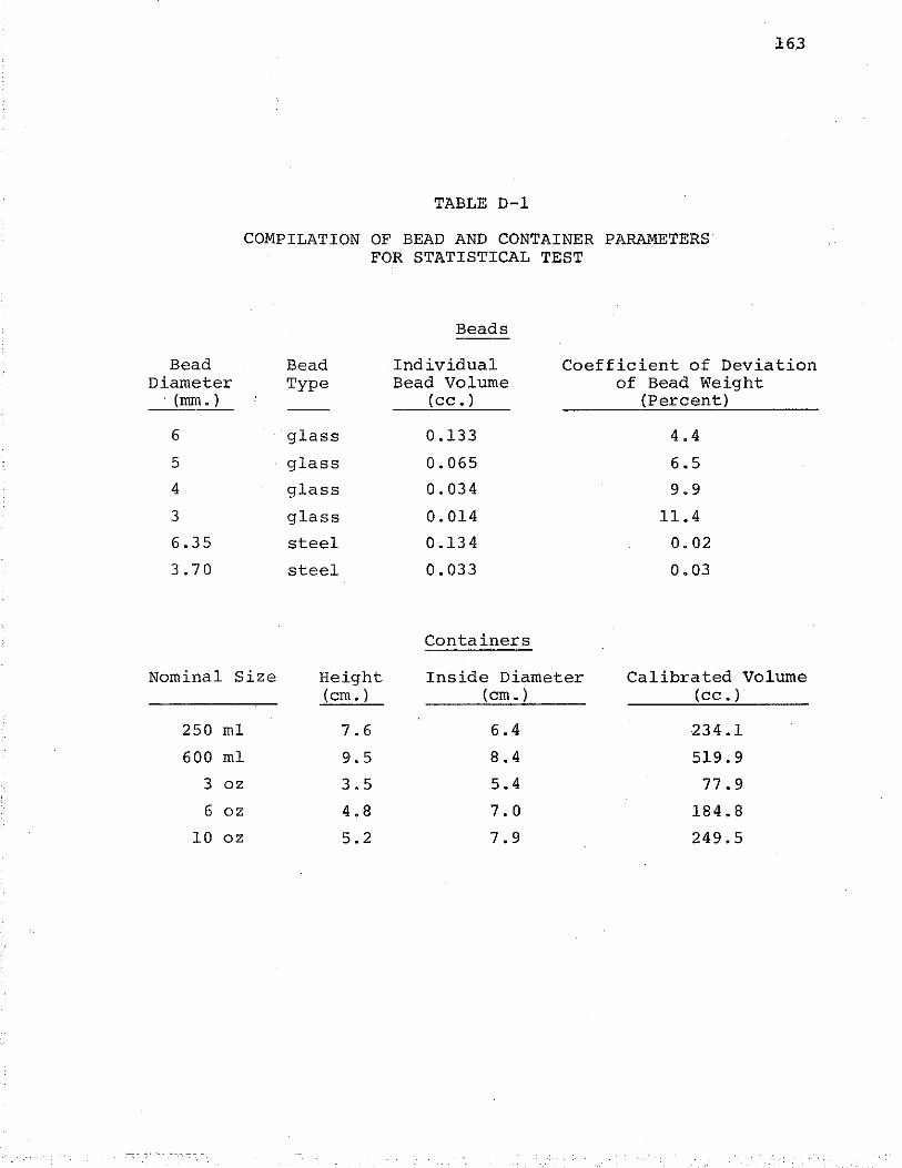
Bead Diameter
. (rom.)
6
5
4
3
6.35
3.70
TABLE D-1
COMPILATION OF BEAD AND CONTAINER PARAMETERS FOR STATISTICAL TEST
Beads
163
Bead Individual Coefficient of Deviation Type Bead Volume of Bead Weight
( cc.) (Percent)
glass 0.133 4.4
glass 0.065 6.5
glass 0.034 9.9
glass 0.014 11.4
steel 0.134 0.02
steel 0.033 0.03
Containers
Nominal Size Height Inside Diameter Calibrated Volume (em.) (em.) (cc.)
250 ml 7.6 6.4 234.1
600 ml 9.5 8.4 519.9
3 oz 3.5 5.4 77.9
6 oz 4.8 7.0 184.8
10 oz 5.2 7.9 249.5
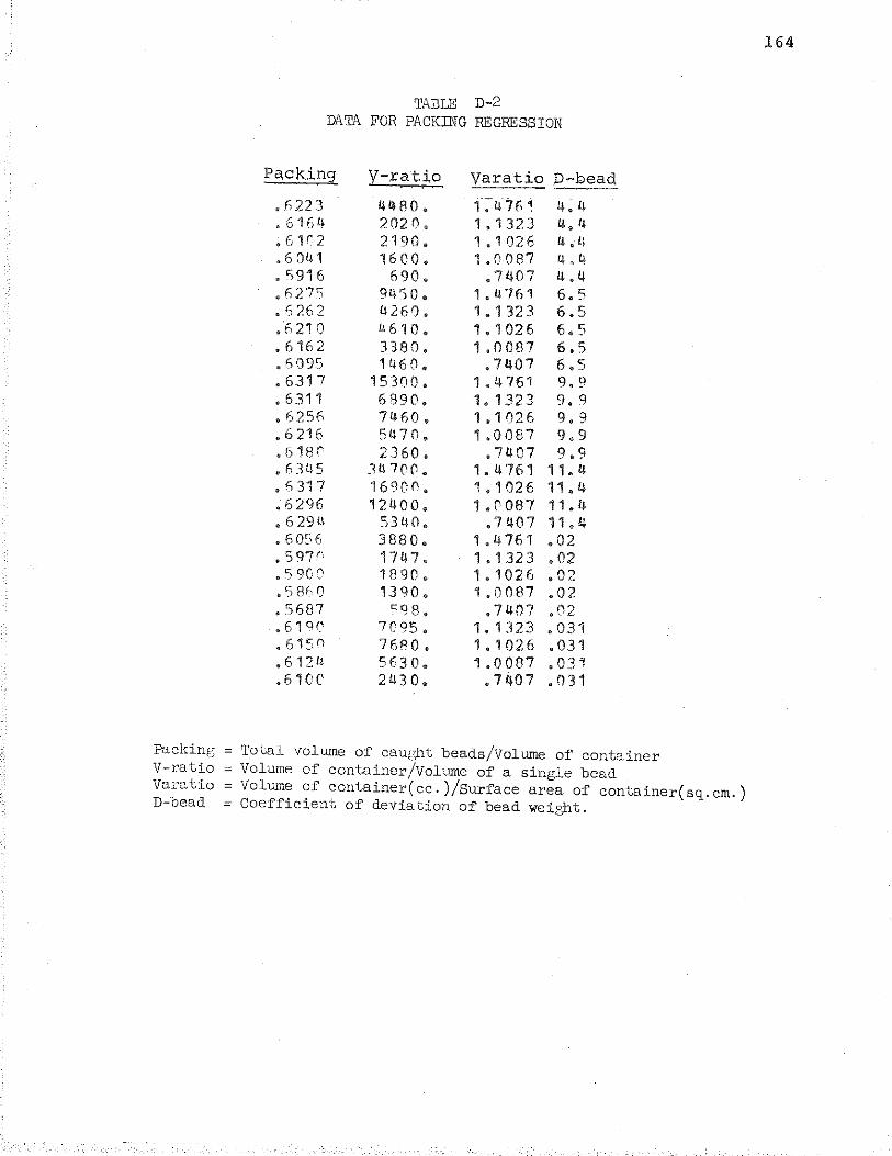
TABLE D-2 DATA FOR PACKING REGRESSION
P2\CJ<;i.ng v-rat;i.o Varat;i.o D~bead
• 622 3 4!180 • 1~4'761 4,4 &6164 202 n, 1. 132 3 U,4 • 61r2 2190 • 1 • , 02 6 U g. L~
• 6 041 1600 • 1.0087 4. 4 • 594 6 690 • • 7407 U,4 .fi27~ 91.+50,.. 1. 4 761 6.5 • 6 26 2 4260 • 1 • 1 32 3 6.5 • h 21 0 4610. 1 • 1 02 6 6.5 .6162 338ri, 1.0087 6,5 • 6095 1460 • • 7407 6.5 • 6317 153r!O, 1. 4 761 9,9 .6311 6890, 1. 1323 9. 9 • 6256 7460, 1.1 026 C). 9 • 6 216 5470 • 1.0087 9.9 • 5180 2360 • .7407 9.9 • 6345 3470(1 • 1. 4 761 , 1. 4 • fi 317 16900, 1 • 1 02 6 11. 4 • 6296 12400 • 1.C087 11.4 • 6 294 531!0, • 7 407 11.4 • 6056 3880 • 1. 4 761 .02 . s 97" 174 7 • 1 • 132 3 .02 • 'i9CO 18 90 • 1.1026 QI02 "5 86 0 1390. 1.0087 .02 • 5687 ~9 8' • 7407 .02 • 61Q(1 7095 • 1. 1323 • 031 ~ 61:)0 7680. 1,1026 .031 • 6121• 563 o • 4.0087 o031 • 61CC 2 4 3 0 • • 7407 ,()31
Packinc; = Total volume of caught beads/Volume of container V-ratio = Volume of container/Volt~e of a single bead Varatio = Volume of container( cc. ) /Surface area of container( sq. em. ) D-bead = Coefficient of deviation of bead weight.
164
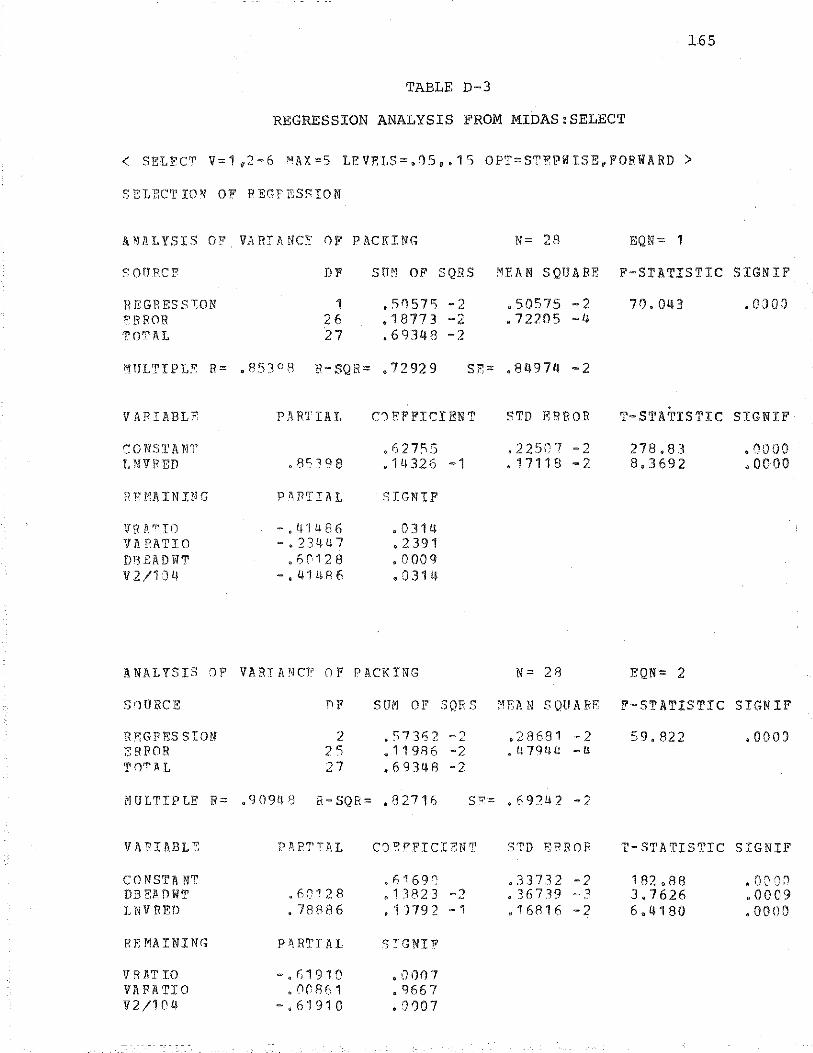
165
TABLE D-3
REGRESSION ANALYSIS FROM MIDAS:SELECT
< SELFC~ V=1 ,2-6 MAX=S LEVEL$=,05,.15 OPT=STEPIISE,FORWARD >
SELHCTIO• OF REGFHSSION
UrALYSIS OF VARIANCE 0F PACKING N= 28 EQN= , S0fl.HCF DF S U!'! OP SQRS MEAN S QUA llE F-SrATISTIC SIGN IF
REGRESSION 1 ,51157') -2 ,50575 -2 70.043 .OJOJ FHROll 26 .18773 -2 .72205 -4 TO'CH 27 .69348 -2
"'UL'ri PLF R= .8530fl H-SQR= • 7 2 92 9 sr:= .84974 -2
VAPIABLB PARTIAL CJEFFICIENT STD ERROR T-STATISTIC SIGN IF
CONSTI\N~ ,02755 • 2 250 7 -2 278,83 ~0000 T.NVPED • 85<98 • 1 4 32 6 -1 .17118 ~ 8.3692 • 0000 -,<.
HE t1l\ IN ING P~RTIAL :) IGNIP
1fR~."'IO -.411J86 .0311.1 VA Rl\1'1.0 -.23447 • 2 391 D~'l El\ D WT .60128 • 0 00 g v 2/1 J 4 -.411+86 .0314
ANALYSIS OP VARIANCP OF PACKING N = 28 EQN= 2
S'JURCE "flF SUM OF SQR S ~lf:A N S QUA FP F-STATISTIC SIGNIF
RF.GPES SION ERROR TOTAL
2 2"i 27
MULTIPLE R= .90948 R- SQR=
VA"'?If\BLE PP.PTIAL
CONSTANT DB F.P. D WT .6()128 lNVRETl • 78886
REMAINING P~RTTAl
V RAT I0 -.fi1910 I' A llATIO .11(1861 V2/1 f\4 -.61910
.S73<;2 -2
.11986 -2 ,69348 -2
,82716 S:;'-::::
C:J~fi'FICIF.:NT
.f;"!69-';
.13823 -2 • 1 ")792 -1
s TGNIF
,001)7 • %67 • ') 007
.28681 -2 59. 82 2 .0003 • 4 7944 -U
• 69:?42 -2
STD BRHOR T-STATISTIC SIGNIF
.33732 -2 1 82 • 8 8 o00!JJ • 3 6 719 -.~ 3.7626 .0009 ,16816 -2 6.4180 ,0000
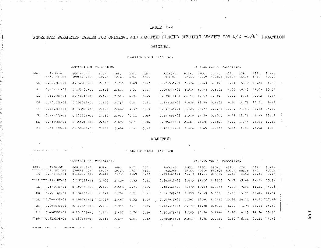
TABLE D-4
AGGREGATE PARI\METER TABLES FOR ORIGINAL AND ADJUSTED PACKING SPECIFIC GR!\VITY FOR 1/2"-5/8" FRACTION
~v'-"·'--·,:c 0:"l·, I • ..,::_ j:__,b:
u:.. {.. ·,·JylJt:+Jl
S$
CG
s l
LS
ss
··-gp -~-u-.SlJlOt:TJl
i:'Jl' I V :..1_ ~ ~;l sr-i,:. c..:~ <JI ; .•
J.l5542l:+01
C~l'5Cll'+Ol
U.l5070H·C l
0~ 15SJl:c+Cl
£:\)1) i V ~LEN i s;'H;:=R~ o:.\. ~J.l53l':J~+Jl
o. b7")lt+Ol
o.l5c8i)2+01
Q.15737ET01
jl_I~J.
:;..>.Gt<.
2. t1U2.
.?. t c;::.
2,.c::.o
lllJ Li\ SP~ (;.{ 2. ,.1;:.
z. J02
2.179
:::.691
2.656
z. dZS
2.7?2
2 .. '}31
SP.C~
l..72D
2..568
2" 7'J.~
ORIGINAL
Ft<-4CT1DN SILt: i/2- ';;/6
l. (; ')
0.33
J .J l
.c... 3 2
. l. !.1
t..SP. :,,_\ :~.
0. 3.'
0.21
0. 51
3. t.,•J
-J.Q5
J. 3 t,
J.32
,•.;,c.,<,.r.-.c; 1/'il :j ;.;
G.l'/~ulF+-)1 2.3t3
O.l97llt+JL 2.628
ADJUSTED
f-KACrlON S!LE: l/2- 5/8
lr'~.4·-J J.c351 3.2i
ll.4b J. d:::52
:..n
1 1..:.,.71 93.31
::~:;;.' . ~ UG. '-'
10.::.3
PACKiNG VOLUME PAKh~ETE~S
',.,'/. T" ;.F.s. l.t.9
J. 3:3
0.53
~~s ~-.
:.ss. PAC KIN::; VJLU~1E
0~ t'/Q;,f:>r;:f-Ol
?.I:.CK~
s P. z;"-2.419
:;1-"- !C:C. :-:·JG. v L l .. <':> t
GEOM. Fc.C TC::; ~-~:S~')
O.l8556E+Ol 2.072 19.33 0.3067
0.19L7JErOl 2.353 !4.49 0.2551
0.20405E+Ol 2~539 5.76 8.9424
ASP. f{U~.w
3.54
ASP~
KUS-.V SJRF .. R:..IG. V 1'.52
5.96 L3.75 9~ .. 8~ 12.57
APPENPIX E
SELECTION OF OPTIMUM ASPHALT CONTENT FROM PESIGN TABLES
An acceptable procedure for selection of optimum
asphalt content using the design tables produced by the
design table program is as follows:
{a) Obtain actual mix specific gravities for a
variety of asphalt contents. Specimens made
in conformance with Marshall specifications are
convenient for this purpose. The range of
asphalt contents considered should ideally have
as its mean the optimum content. A good esti
mation for optimum asphalt content can be made
from analysis of the design tables alone.
(b) Enter the design tables at ·the respective asphalt
contents and mix specific gravities as obtained
from the experimental specimens. ··At these_points,
note and record the packing V.M.A. calculated by
the design table program.
{c) Plot packing V.M.A. versus asphalt content.
Tests to date have shown that optimum asphalt
content is indicated at minimum packing V.M.A.
(d) In some cases, packing V.M.A. will not reach a
minimum, but will continue to decrease as asphalt
content is increased. In such cases, asphalt
167
168
optimum prediction should be made based on the
value chosen for minimum air voids. This value I
may vary. The air void value used herein is the
value used by the Michigan Department of State
Highways and Transportation, 4%.
Figure E-1 shows a typical example of the relation-
ship between Marshall data and computed packing V.M.A.
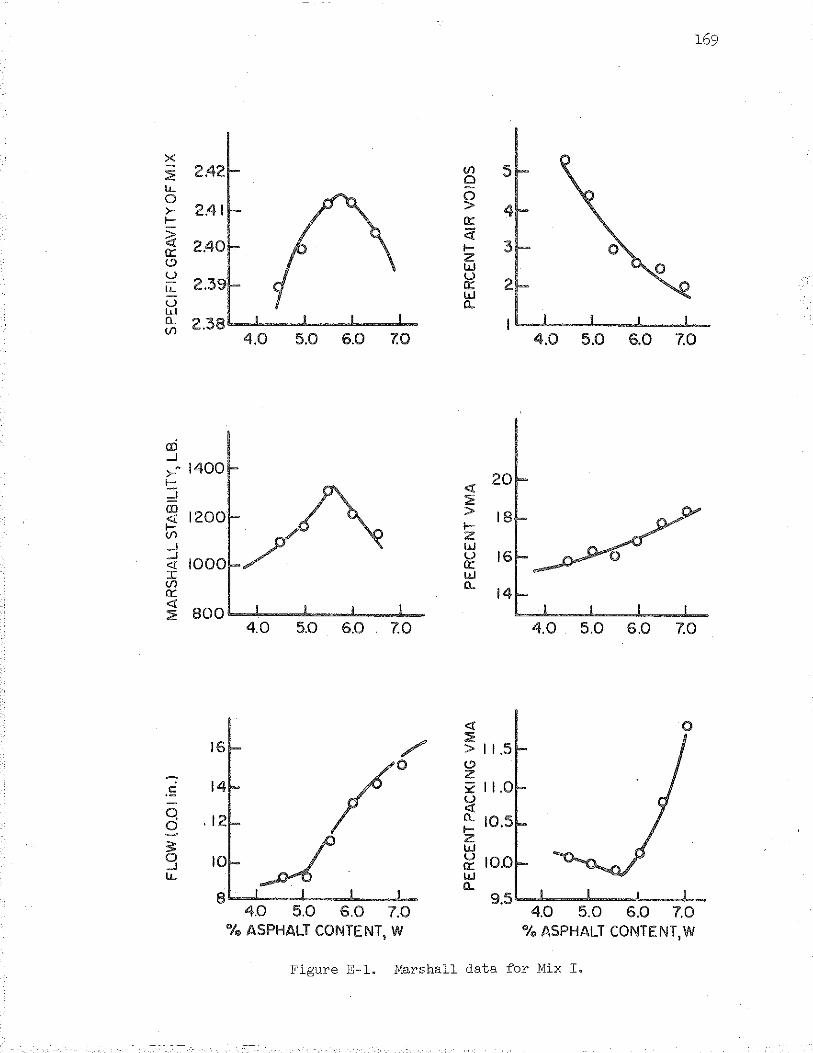
>< ::1: 2.42 u.. 0 >- 2.41 1-
~ 2.40 0::: <.:> u u.. u w a.. 2.38 (/)
ai ....! >-" 1400 1-:i <D
f5! (/)
....!
....! < I (/)
0::: q
BOO ::1:
16
-.E 14
Q 0
3: 0 ....! 1.1..
8
4.0 5.0 6.0 7.0
4.0 5.0 6.0 7.0
/ /0 ~
4.0 5.0 6.0 7.0 %ASPHALT CONTENT, W
(/) 0 0 > 0::: ;:{ 1-z w u 0::: w CL
<l: ::1: > 1-z w u 0::: w a..
q ::1:
5
4
3
2
20
18
16
14
> 11.5
1-z w u 0::: w CL
169
4.0 5.0 6.0 7.0
4.0 5.0 6.0 7.0
4.0 5.0 6.0 7.0 %ASPHALT CONTENT, W
Figure E-l. Marshall data for Mix I.


