
Chapter 14
Ruled Surfaces
We describe in this chapter the important class of surfaces, consistng of those
which contain infinitely many straight lines. The most obvious examples of
ruled surfaces are cones and cylinders (see pages 314 and 375).
Ruled surfaces are arguably the easiest of all surfaces to parametrize. A
chart can be defined by choosing a curve in R3 and a vector field along that
curve, and the resulting parametrization is linear in one coordinate. This is the
content of Definition 14.1, that provides a model for the definition of both the
helicoid and the Mobius strip (described on pages 376 and 339).
Several quadric surfaces, including the hyperbolic paraboloid and the hyper-
boloid of one sheet are also ruled, though this fact does not follow so readily from
their definition. These particular quadric surfaces are in fact ‘doubly ruled’ in
the sense that they admit two one-parameter families of lines. In Section 14.1,
we explain how to parametrize them in such a way as to visualize the straight
line rulings. We also define the Plucker conoid and its generalizations.
It is a straightforward matter to compute the Gaussian and mean curvature
of a ruled surface. This we do in Section 14.2, quickly turning attention to flat
ruled surfaces, meaning ruled surfaces with zero Gaussian curvature. There are
three classes of such surfaces, the least obvious but most interesting being the
class of tangent developables.
Tangent developables are the surfaces swept out by the tangent lines to a
space curve, and the two halves of each tangent line effectively divide the surface
into two sheets which meet along the curve in a singular fashion described by
Theorem 14.7. This behaviour is examined in detail for Viviani’s curve, and
the linearity inherent in the definition of a ruled surface enables us to highlight
the useful role played by certain plane curves in the description of tangent
developables.
In the final Section 14.4, we shall study a class of surfaces that will help us
to better understand how the Gaussian curvature varies on a ruled surface.
431
432 CHAPTER 14. RULED SURFACES
14.1 Definitions and Examples
A ruled surface is a surface generated by a straight line moving along a curve.
Definition 14.1. A ruled surface M in R3 is a surface which contains at least
one 1-parameter family of straight lines. Thus a ruled surface has a parame-
trization x : U → M of the form
x(u, v) = α(u) + vγ(u),(14.1)
where α and γ are curves in R3. We call x a ruled patch. The curve α is called
the directrix or base curve of the ruled surface, and γ is called the director curve.
The rulings are the straight lines v 7→ α(u) + vγ(u).
In using (14.1), we shall assume that α′ is never zero, and that γ is not identi-
cally zero.
We shall see later that any straight line in a surface is necessarily an as-
ymptotic curve, pointing as it does in direction for which the normal curvature
vanishes (see Definition 13.9 on page 390 and Corollary 18.6 on page 560). It
follows that the rulings are asymptotic curves. Sometimes a ruled surface Mhas two distinct ruled patches on it, so that a ruling of one patch does not
belong to the other patch. In this case, we say that x is doubly ruled.
We now investigate a number of examples.
The Helicoid and Mobius Strip Revisited
We can rewrite the definition (12.27) as
helicoid[a, b](u, v) = α(u) + vγ(u),
where {α(u) = (0, 0, bu),
γ(u) = a(cos u, sinu, 0).(14.2)
In this way, helicoid[a, b] is a ruled surface whose base curve has the z-axis as its
trace, and director curve γ that describes a circle.
In a similar fashion, our definition (11.3), page 339, of the Mobius strip
becomes
moebiusstrip(u, v) = α(u) + vγ(u),
where
α(u) = (cosu, sin u, 0),
γ(u) =(
cosu
2cosu, cos
u
2sin u, sin
u
2
).
(14.3)
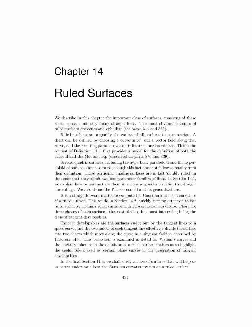
This time, it is the circle that is the base curve of the ruled surface. The Mobius
strip has a director curve γ which lies on a unit sphere, shown in two equivalent
ways in Figure 14.1.
14.1. DEFINITIONS AND EXAMPLES 433
Figure 14.1: Director curve for the Mobius strip
The curve γ is not one that we encountered in the study of curves on the sphere
in Section 8.4. It does however have the interesting property that whenever p
belongs to its trace, so does the antipodal point −p.
The Hyperboloid of One Sheet
We have seen that the elliptical hyperboloid of one sheet is defined nonparamet-
rically byx2
a2+
y2
b2− z2
c2= 1.(14.4)
Planes perpendicular to the z-axis intersect the surface in ellipses, while planes
parallel to the z-axis intersect it in hyperbolas. We gave the standard parame-
trization of the hyperboloid of one sheet on page 313, but this has the disad-
vantage of not showing the rulings.
Let us show that the hyperboloid of one sheet is a doubly-ruled surface by
finding two ruled patches on it. This can be done by fixing a, b, c > 0 and
defining
x±(u, v) = α(u) ± vα′(u) + v (0, 0, c),
where
α(u) = ellipse[a, b](u) = (a cosu, b sinu, 0).(14.5)
is the standard parametrization of the ellipse
x2
a2+
y2
b2= 1
in the xy-plane. It is readily checked that
x±(u, v) =(a(cosu ∓ v sin u), b(sinu ± v cosu), cv
),(14.6)
434 CHAPTER 14. RULED SURFACES
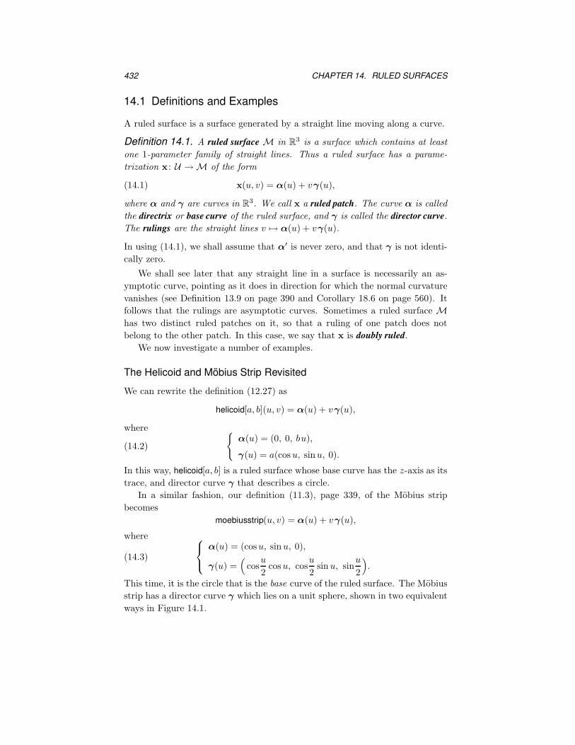
and that both x+ and x− are indeed parametrizations of the hyperboloid (14.4).
Hence the elliptic hyperboloid is doubly ruled; in both cases, the base curve can
be taken to be the ellipse (14.5). We also remark that x+ can be obtained from
x− by simultaneously changing the signs of the parameter c and the variable v.
Figure 14.2: Rulings on a hyperboloid of one sheet
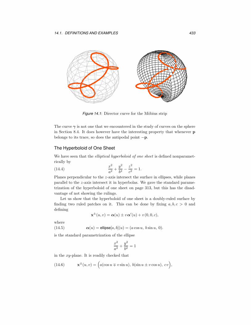
The Hyperbolic Paraboloid
The hyperbolic paraboloid is defined nonparametrically by
z =x2
a2− y2
b2(14.7)
(though the constants a, b here are different from those in (10.16)). It is doubly
ruled, since it can be parametrized in the two ways
x±(u, v) = (au, 0, u2) + v(a, ±b, 2u)
= (a(u + v), ±bv, u2 + 2uv).
Although we have tacitly assumed that b > 0, both parametrizations can ob-
viously be obtained from the same formula by changing the sign of b, a fact
exploited in Notebook 14.
A special case corresponds to taking a = b and carrying out a rotation by
π/2 about the z-axis, so as to define new coordinates
x =1√
2(x − y)
y =1√
2(x + y),
z = z.
This transforms (14.7) into the equation a2z = 2 xy.
14.1. DEFINITIONS AND EXAMPLES 435
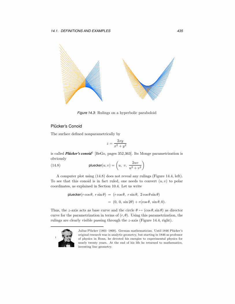
Figure 14.3: Rulings on a hyperbolic paraboloid
Plucker’s Conoid
The surface defined nonparametrically by
z =2xy
x2 + y2
is called Plucker’s conoid1 [BeGo, pages 352,363]. Its Monge parametrization is
obviously
pluecker(u, v) =
(u, v,
2uv
u2 + v2
)(14.8)
A computer plot using (14.8) does not reveal any rulings (Figure 14.4, left).
To see that this conoid is in fact ruled, one needs to convert (u, v) to polar
coordinates, as explained in Section 10.4. Let us write
pluecker(r cos θ, r sin θ) = (r cos θ, r sin θ, 2 cos θ sin θ)
= (0, 0, sin 2θ) + r(cos θ, sin θ, 0).
Thus, the z-axis acts as base curve and the circle θ 7→ (cos θ, sin θ) as director
curve for the parametrization in terms of (r, θ). Using this parametrization, the
rulings are clearly visible passing through the z-axis (Figure 14.4, right).
1
Julius Plucker (1801–1868). German mathematician. Until 1846 Plucker’s
original research was in analytic geometry, but starting in 1846 as professor
of physics in Bonn, he devoted his energies to experimental physics for
nearly twenty years. At the end of his life he returned to mathematics,
inventing line geometry.

436 CHAPTER 14. RULED SURFACES
Figure 14.4: Parametrizations of the Plucker conoid
It is now an easy matter to define a generalization of Plucker’s conoid that
has n folds instead of 2:
plueckerpolar[n](r, θ) = (r cos θ, r sin θ, sin nθ).(14.9)
Each surface plueckerpolar[n] is a ruled surface with the rulings passing through
the z-axis. For a generalization of (14.9) that includes a variant of the monkey
saddle as a special case, see Exercise 5.
Even more general than (14.9) is the right conoid, which is a ruled surface
with rulings parallel to a plane and passing through a line that is perpendicular
to the plane. For example, if we take the plane to be the xy-plane and the line
to be the z-axis, a right conoid will have the form
rightconoid[ϑ, h](u, v) =(v cosϑ(u), v sin ϑ(u), h(u)
).(14.10)
This is investigated in Notebook 14 and illustrated in Figure 14.12 on page 449.
Figure 14.5: The conoids plueckerpolar[n] with n = 3 and 7
14.2. CURVATURE OF A RULED SURFACE 437
14.2 Curvature of a Ruled Surface
Lemma 14.2. The Gaussian curvature of a ruled surface M ⊂ R3 is every-
where nonpositive.
Proof. If x is a ruled patch on M, then xvv = 0; consequently g = 0. Hence it
follows from Theorem 13.25, page 400, that
K =−f2
EG − F 26 0.(14.11)
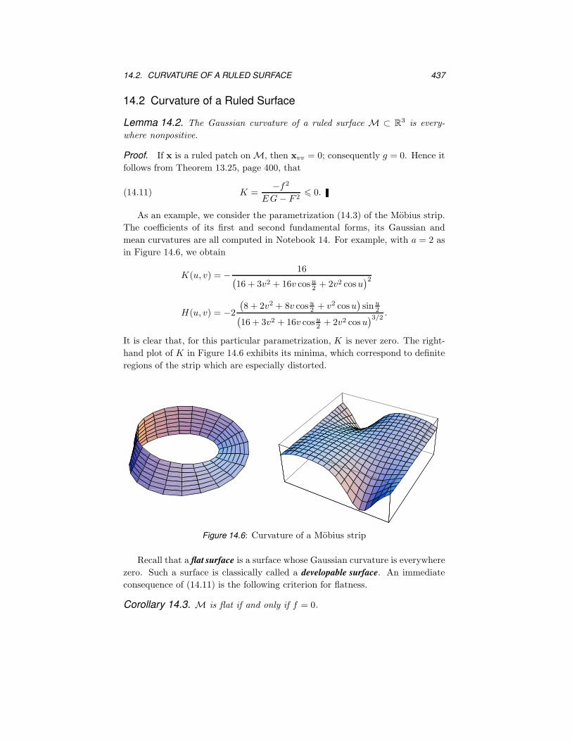
As an example, we consider the parametrization (14.3) of the Mobius strip.
The coefficients of its first and second fundamental forms, its Gaussian and
mean curvatures are all computed in Notebook 14. For example, with a = 2 as
in Figure 14.6, we obtain
K(u, v) = − 16(16 + 3v2 + 16v cosu
2+ 2v2 cosu
)2
H(u, v) = −2
(8 + 2v2 + 8v cosu
2+ v2 cosu
)sin u
2(16 + 3v2 + 16v cosu
2+ 2v2 cosu
)3/2.
It is clear that, for this particular parametrization, K is never zero. The right-
hand plot of K in Figure 14.6 exhibits its minima, which correspond to definite
regions of the strip which are especially distorted.
Figure 14.6: Curvature of a Mobius strip
Recall that a flat surface is a surface whose Gaussian curvature is everywhere
zero. Such a surface is classically called a developable surface. An immediate
consequence of (14.11) is the following criterion for flatness.
Corollary 14.3. M is flat if and only if f = 0.

438 CHAPTER 14. RULED SURFACES
The most obvious examples of flat surfaces, other than the plane, are circular
cylinders and cones (see the discussion after Figure 14.7). Paper models of both
can easily be constructed by bending a sheet of paper and, as we shall see
in Section 17.2, this operation leaves the Gaussian curvature unchanged and
identically zero. Circular cylinders and cones are subsumed into parts (ii) and
(iii) of the following list of flat ruled surfaces.
Definition 14.4. Let M ⊂ R3 be a surface. Then:
(i) M is said to be the tangent developable of a curve α : (a, b) → R3 if M
can be parametrized as
x(u, v) = α(u) + vα′(u);(14.12)
(ii) M is a generalized cylinder over a curve α : (a, b) 7→ R3 if M can be
parametrized as
y(u, v) = α(u) + vq,
where q ∈ R3 is a fixed vector;
(iii) M is a generalized cone over a curve α : (a, b) → R3, provided M can
be parametrized as
z(u, v) = p + vα(u),
where p ∈ R3 is fixed (it can be interpreted as the vertex of the cone).
Our next result gives criteria for the regularity of these three classes of
surfaces. We base it on Lemma 10.18.
Lemma 14.5. (i) Let α : (a, b) → R3 be a regular curve whose curvature κ[α]
is everywhere nonzero. The tangent developable x of α is regular everywhere
except along α.
(ii) A generalized cylinder y(u, v) = α(u) + vq is regular wherever α′ × q
does not vanish.
(iii) A generalized cone z(u, v) = p + vα(u) is regular wherever vα × α′ is
nonzero, and is never regular at its vertex.
Proof. For a tangent developable x, we have
(xu × xv)(u, v) = (α′ + vα′′) × α′ = vα′′ × α′.(14.13)
If κ[α] 6= 0, then α′′×α′ is everywhere nonzero by (7.26). Thus (14.13) implies
that x is regular whenever v 6= 0. The other statements have similar proofs.
14.2. CURVATURE OF A RULED SURFACE 439
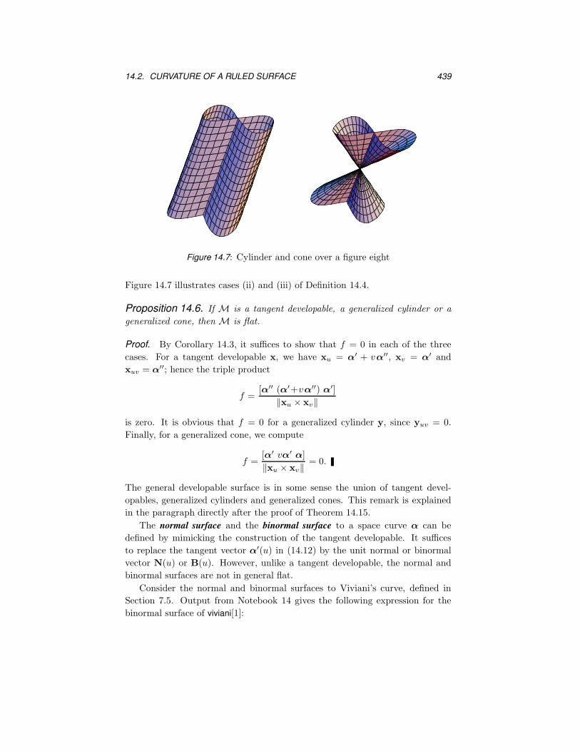
Figure 14.7: Cylinder and cone over a figure eight
Figure 14.7 illustrates cases (ii) and (iii) of Definition 14.4.
Proposition 14.6. If M is a tangent developable, a generalized cylinder or a
generalized cone, then M is flat.
Proof. By Corollary 14.3, it suffices to show that f = 0 in each of the three
cases. For a tangent developable x, we have xu = α′ + vα′′, xv = α′ and
xuv = α′′; hence the triple product
f =[α′′ (α′+vα′′) α′]
‖xu × xv‖
is zero. It is obvious that f = 0 for a generalized cylinder y, since yuv = 0.
Finally, for a generalized cone, we compute
f =[α′ vα′ α]
‖xu × xv‖= 0.
The general developable surface is in some sense the union of tangent devel-
opables, generalized cylinders and generalized cones. This remark is explained
in the paragraph directly after the proof of Theorem 14.15.
The normal surface and the binormal surface to a space curve α can be
defined by mimicking the construction of the tangent developable. It suffices
to replace the tangent vector α′(u) in (14.12) by the unit normal or binormal
vector N(u) or B(u). However, unlike a tangent developable, the normal and
binormal surfaces are not in general flat.
Consider the normal and binormal surfaces to Viviani’s curve, defined in
Section 7.5. Output from Notebook 14 gives the following expression for the
binormal surface of viviani[1]:

440 CHAPTER 14. RULED SURFACES
(1 + cosu +
v(3 sinu
2+ sin 3u
2
)√
26 + 6 cosu,−2
√2v cos3 u
2√13 + 3 cosu
+ sin u,
2√
2v√13 + 3 cosu
+ 2 sinu
2
)
Figure 14.8 shows parts of the normal and binormal surfaces together, with the
small gap representing Viviani’s curve itself. The curvature of these surfaces is
computed in Notebook 14, and shown to be nonzero.
Figure 14.8: Normal and binormal surfaces to Viviani’s curve
14.3 Tangent Developables
Consider the surface
tandev[α] = α(u) + vα′(u);
this was first defined in (14.12), though we now use notation from Notebook 14.
We know from Lemma 14.5 that tandev[α] is singular along the curve α. We
prove next that it is made up of two sheets which meet along the trace of α in
a sharp edge, called the edge of regression.
Theorem 14.7. Let α : (a, b) → R3 be a unit-speed curve with a < 0 < b, and
let x be the tangent developable of α. Suppose that α is differentiable at 0 and
that the curvature and torsion of α are nonzero at 0. Then the intersection of
the trace of x with the plane perpendicular to α at α(0) is approximated by a
semicubical parabola with a cusp at α(0).
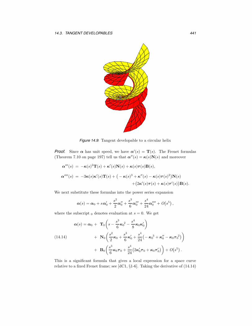
14.3. TANGENT DEVELOPABLES 441
Figure 14.9: Tangent developable to a circular helix
Proof. Since α has unit speed, we have α′(s) = T(s). The Frenet formulas
(Theorem 7.10 on page 197) tell us that α′′(s) = κ(s)N(s) and moreover
α′′′(s) = −κ(s)2T(s) + κ′(s)N(s) + κ(s)τ (s)B(s),
α′′′′(s) = −3κ(s)κ′(s)T(s) +(− κ(s)3 + κ′′(s) − κ(s)τ (s)2
)N(s)
+(2κ′(s)τ (s) + κ(s)τ ′(s)
)B(s).
We next substitute these formulas into the power series expansion
α(s) = α0 + sα′
0 +s2
2α′′
0 +s3
6α′′′
0 +s4
24α′′′′
0 + O(s5),
where the subscript 0 denotes evaluation at s = 0. We get
α(s) = α0 + T0
(s − s3
6κ0
2 − s4
8κ0κ
′
0
)
+ N0
(s2
2κ0 +
s3
6κ′
0 +s4
24
(− κ0
3 + κ′′
0 − κ0τ 02))
+ B0
(s3
6κ0τ 0 +
s4
24
(2κ′
0τ 0 + κ0τ′
0
))+ O
(s5).
(14.14)
This is a significant formula that gives a local expression for a space curve
relative to a fixed Frenet frame; see [dC1, §1-6]. Taking the derivative of (14.14)
442 CHAPTER 14. RULED SURFACES
gives
α′(s) = T0
(1 − s2
2κ0
2 − s3
2κ0κ
′
0
)
+ N0
(sκ0 +
s2
2κ′
0 +s3
6
(− κ0
3 + κ′′
0 − κ0τ 02))
+ B0
(s2
2κ0τ 0 +
s3
6
(2κ′
0τ 0 + κ0τ′
0
))+ O
(s4).
The tangent developable of α is therefore given by
x(u, v) = α(u) + vα′(u)
= α0 + T0
(u − u3
6κ0
2 + v − u2v
2κ0
2 − u3v
2κ0κ
′
0
)
+ N0
(u2
2κ0 +
u3
6κ′
0 + uvκ0 +u2v
2κ′
0 +u3v
6
(− κ0
3 + κ′′
0 − κ0τ 02))
+B0
((u3
6+
u2v
2
)κ0τ 0 +
u3v
6
(2κ′
0τ 0 + κ0τ′
0
))+ O
(u4).
We want to determine the intersection of x with the plane perpendicular to α
at α0. Therefore, we set the above coefficient of T0 equal to zero and solve for
v to give
v = −u − 1
6u3κ0
2 + O(u4)
1 − 1
2u2κ0
2 − 1
2u3κ0κ
′
0 + O(u4) = −u − κ0
2 u3
3+ O
(u4).
Substituting back this value yields the following power series expansions:
x = coefficient of N0 = −u2
2κ0 − · · ·
y = coefficient of B0 = −u3
3κ0τ 0 + · · ·
(14.15)
By hypothesis, κ0 6= 0 6= τ 0, so that we can legitimately ignore higher order
terms. Doing this, the plane curve described by (14.15) is approximated by the
implicit equation
8τ 02 x3 + 9κ0 y2 = 0,
which is a semicubical parabola.
14.3. TANGENT DEVELOPABLES 443
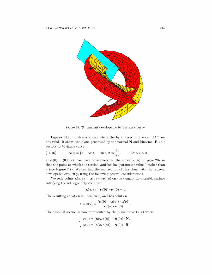
Figure 14.10: Tangent developable to Viviani’s curve
Figures 14.10 illustrates a case where the hypotheses of Theorem 14.7 are
not valid. It shows the plane generated by the normal N and binormal B unit
vectors to Viviani’s curve
α(t) =(1 − cos t, − sin t, 2 cos
t
2
), −3π 6 t 6 π(14.16)
at α(0) = (0, 0, 2). We have reparametrized the curve (7.35) on page 207 so
that the point at which the torsion vanishes has parameter value 0 rather than
π (see Figure 7.7). We can find the intersection of this plane with the tangent
developable explicitly, using the following general considerations.
We seek points x(u, v) = α(u) + vα′(u) on the tangent developable surface
satisfying the orthogonality condition
(x(u, v) − α(0)) · α′(0) = 0.
The resulting equation is linear in v, and has solution
v = v(u) =(α(0) − α(u)) · α′(0)
α′(u) · α′(0).
The cuspidal section is now represented by the plane curve (x, y) where{
x(u) = (x(u, v(u)) − α(0)) · N,
y(u) = (x(u, v(u)) − α(0)) · B.
444 CHAPTER 14. RULED SURFACES
-4 -3 -2 -1
1.8
1.9
2.1
2.2
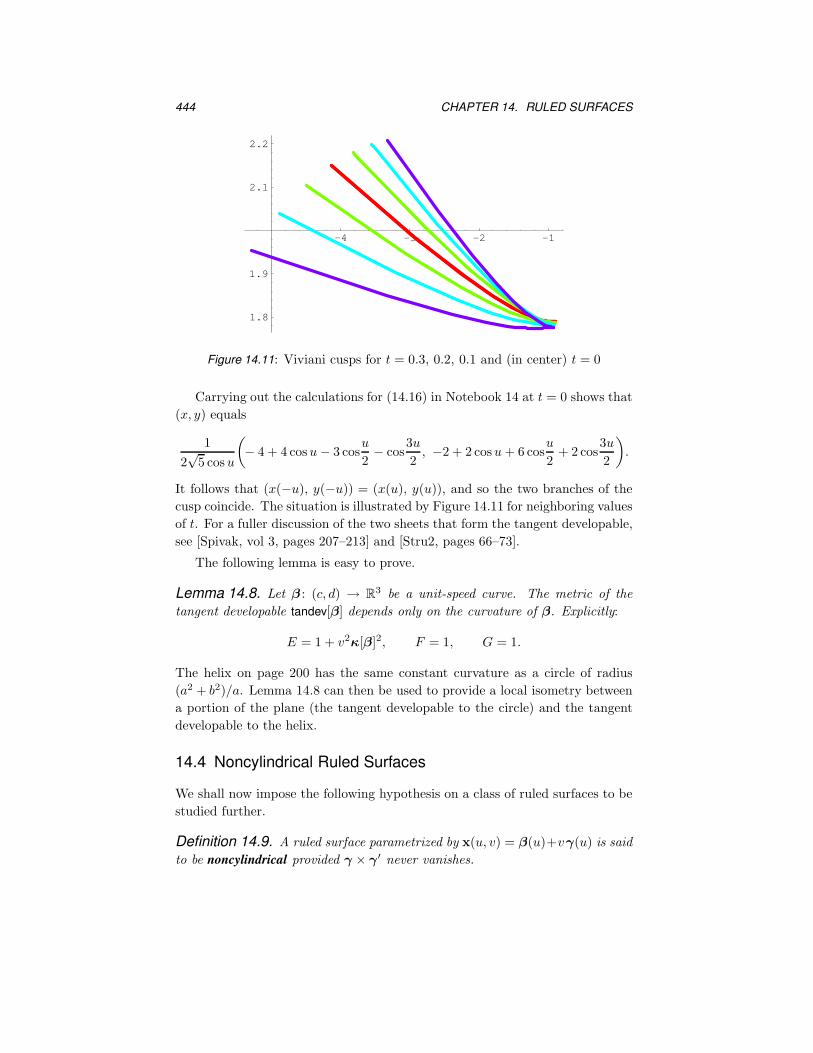
Figure 14.11: Viviani cusps for t = 0.3, 0.2, 0.1 and (in center) t = 0
Carrying out the calculations for (14.16) in Notebook 14 at t = 0 shows that
(x, y) equals
1
2√
5 cosu
(− 4 + 4 cosu − 3 cos
u
2− cos
3u
2, −2 + 2 cosu + 6 cos
u
2+ 2 cos
3u
2
).
It follows that (x(−u), y(−u)) = (x(u), y(u)), and so the two branches of the
cusp coincide. The situation is illustrated by Figure 14.11 for neighboring values
of t. For a fuller discussion of the two sheets that form the tangent developable,
see [Spivak, vol 3, pages 207–213] and [Stru2, pages 66–73].
The following lemma is easy to prove.
Lemma 14.8. Let β : (c, d) → R3 be a unit-speed curve. The metric of the
tangent developable tandev[β] depends only on the curvature of β. Explicitly:
E = 1 + v2κ[β]2, F = 1, G = 1.
The helix on page 200 has the same constant curvature as a circle of radius
(a2 + b2)/a. Lemma 14.8 can then be used to provide a local isometry between
a portion of the plane (the tangent developable to the circle) and the tangent
developable to the helix.
14.4 Noncylindrical Ruled Surfaces
We shall now impose the following hypothesis on a class of ruled surfaces to be
studied further.
Definition 14.9. A ruled surface parametrized by x(u, v) = β(u)+vγ(u) is said
to be noncylindrical provided γ × γ′ never vanishes.

14.4. NONCYLINDRICAL RULED SURFACES 445
The rulings are always changing directions on a noncylindrical ruled surface.
We show how to find a useful reference curve on a noncylindrical ruled surface.
This curve, called a striction curve, is a generalization of the edge of regression
of a tangent developable.
Lemma 14.10. Let x be a parametrization of a noncylindrical ruled surface of
the form x(u, v) = β(u) + vγ(u). Then x has a reparametrization of the form
x(u, v) = σ(u) + vδ(u),(14.17)
where ‖δ‖ = 1 and σ′· δ′ = 0. The curve σ is called the striction curve of x.
Proof. Since γ×γ′ is never zero, γ is never zero. We define a reparametrization˜x of x by
˜x(u, v) = x
(u,
v
‖γ(u)‖)
= β(u) +vγ(u)
‖γ(u)‖ .
Clearly, ˜x has the same trace as x. If we put δ(u) = γ(u)/‖γ(u)‖, then
˜x(u, v) = β(u) + vδ(u).
Furthermore, ‖δ(u)‖ = 1 and so δ(u) · δ′(u) = 0.
Next, we need to find a curve σ such that σ′(u) · δ′(u) = 0. To this end, we
write
σ(u) = β(u) + t(u)δ(u)(14.18)
for some function t = t(u) to be determined. We differentiate (14.18), obtaining
σ′(u) = β′(u) + t′(u)δ(u) + t(u)δ′(u).
Since δ(u) · δ′(u) = 0, it follows that
σ′(u) · δ′(u) = β′(u) · δ′(u) + t(u)δ′(u) · δ′(u).
Since γ × γ′ never vanishes, γ and γ′ are always linearly independent, and
consequently δ′ never vanishes. Thus if we define t by
t(u) = −β′(u) · δ′(u)
‖δ′(u)‖2,(14.19)
we get σ′(u) · δ′(u) = 0. Now define
x(u, v) = ˜x(u, t(u) + v).
Then x(u, v) = β(u) + (t(u) + v)δ(u) = σ(u) + vδ(u), so that x, x and ˜x all
have the same trace, and x satisfies (14.17).
446 CHAPTER 14. RULED SURFACES
Lemma 14.11. The striction curve of a noncylindrical ruled surface x does
not depend on the choice of base curve.
Proof. Let β and β be two base curves for x. In the notation of the previous
proof, we may write
β(u) + vδ(u) = β(u) + w(v)δ(u)(14.20)
for some function w = w(v). Let σ and σ be the corresponding striction curves.
Then
σ(u) = β(u) − β′(u) · δ′(u)
‖δ′(u)‖2δ(u)
and
σ(u) = β(u) − β′
(u) · δ′(u)
‖δ′(u)‖2δ(u),
so that
σ − σ = β − β − (β′ − β′
) · δ′
‖δ′‖2δ.(14.21)
On the other hand, it follows from (14.20) that
β − β = (w(v) − v)δ.(14.22)
The result follows by substituting (14.22) and its derivative into (14.21).
There is a nice geometric interpretation of the striction curve σ of a ruled
surface x, which we mention without proof. Let ε > 0 be small. Since nearby
rulings are not parallel to each other, there is a unique point P (ε) on the straight
line v 7→ x(u, v) that is closest to the line v 7→ x(u+ε, v). Then P (ε) → σ(u) as
ε → 0. This follows because (14.19) is the equation that results from minimizing
‖σ′‖ to first order.
Definition 14.12. Let x be a noncylindrical ruled surface given by (14.17).
Then the distribution parameter of x is the function p = p(u) defined by
p =[σ′ δ δ′]
δ′· δ′
.(14.23)
Whilst the definition of σ requires σ′ to be perpendicular to δ′, the function
p measures the component of σ′ perpendicular to δ × δ′.
Lemma 14.13. Let M be a noncylindrical ruled surface, parametrized by a
patch x of the form (14.17). Then x is regular whenever v 6= 0, or when v = 0
and p(u) 6= 0. Furthermore, the Gaussian curvature of x is given in terms of
its distribution parameter by
K =−p(u)2
(p(u)2 + v2
)2 .(14.24)
14.4. NONCYLINDRICAL RULED SURFACES 447
Also,
E = ‖σ′‖2 + v2‖δ′‖2, F = σ′· δ, G = 1,
EG − F 2 = (p2 + v2)‖δ′‖2,
and
g = 0, f =p‖δ′‖√p2 + v2
.
Proof. First, we observe that both σ′ × δ and δ′ are perpendicular to both δ
and σ′. Therefore, σ′ × δ must be a multiple of δ′, and
σ′ × δ = pδ′ where p =[σ′ δ δ′]
δ′· δ′
.
Since xu = σ′ + vδ′ and xv = δ, we have
xu × xv = pδ′ + vδ′ × δ,
so that
‖xu × xv‖2 = ‖pδ′‖2 + ‖vδ′ × δ‖2 = (p2 + v2)‖δ′‖2.
It is now clear that the regularity of x is as stated.
Next, xuv = δ′ and xvv = 0, so that g = 0 and
f =[xuv xu xv]
‖xu × xv‖=
δ′· (pδ′ + vδ′ × δ)√
p2 + v2‖δ′‖=
p‖δ′‖√p2 + v2
.
Therefore,
K =−f2
‖xu × xv‖2=
−(
p‖δ′‖√p2 + v2
)2
(p2 + v2)‖δ′‖2,
which simplifies into (14.24).
Equation (14.24) tells us that the Gaussian curvature of a noncylindrical
ruled surface is generally negative. However, more can be said.
Corollary 14.14. Let M be a noncylindrical ruled surface given by (14.17) with
distribution parameter p, and Gaussian curvature K(u, v).
(i) Along a ruling (so u is fixed), K(u, v) → 0 as v → ∞.
(ii) K(u, v) = 0 if and only if p(u) = 0.
(iii) If p never vanishes, then K(u, v) is continuous and |K(u, v)| assumes its
maximum value 1/p2 at v = 0.
Proof. All of these statements follow from (14.24).
448 CHAPTER 14. RULED SURFACES
Next, we prove a partial converse of Proposition 14.6.
Theorem 14.15. Let x(u, v) = β(u) + vδ(u) with ‖δ(u)‖ = 1 parametrize a
flat ruled surface M.
(i) If β′(u) ≡ 0, then M is a cone.
(ii) If δ′(u) ≡ 0, then M is a cylinder.
(iii) If both β′ and δ′ never vanish, then M is the tangent developable of its
striction curve.
Proof. Parts (i) and (ii) are immediate from the definitions, so it suffices to
prove (iii). We can assume that β is a unit-speed striction curve, so that
β′· δ′ ≡ 0.(14.25)
Since K ≡ 0, it follows from (14.24) and (14.23) that
[β′ δ δ′] ≡ 0.(14.26)
Then (14.25) and (14.26) imply that β′ and δ are collinear.
Of course, cases (i), (ii) and (iii) of Theorem 14.15 do not exhaust all of
the possibilities. If there is a clustering of the zeros β or δ, the surface can be
complicated. In any case, away from the cluster points a developable surface
is the union of pieces of cylinders, cones and tangent developables. Indeed,
the following result is proved in [Krey1, page 185]. Every flat ruled patch
(u, v) 7→ x(u, v) can be subdivided into sufficiently small u-intervals so that the
portion of the surface corresponding to each interval is a portion of one of the
following: a plane, a cylinder, a cone, a tangent developable.
Examples of Striction Curves
The parametrization (12.27) of the circular helicoid can be rewritten as
x(u, v) = (0, 0, bu) + av(cos u, sinu, 0),
which shows that it is a ruled surface. The striction curve σ and director curve
δ are given by
σ(u) = (0, 0, bu) and δ(u) = (cos u, sin u, 0).
Then
x
(u,
v
a
)= σ(u) + vδ(u) = (v cosu, v sin u, bu),
and the distribution parameter assumes the constant value b.
14.5. EXERCISES 449
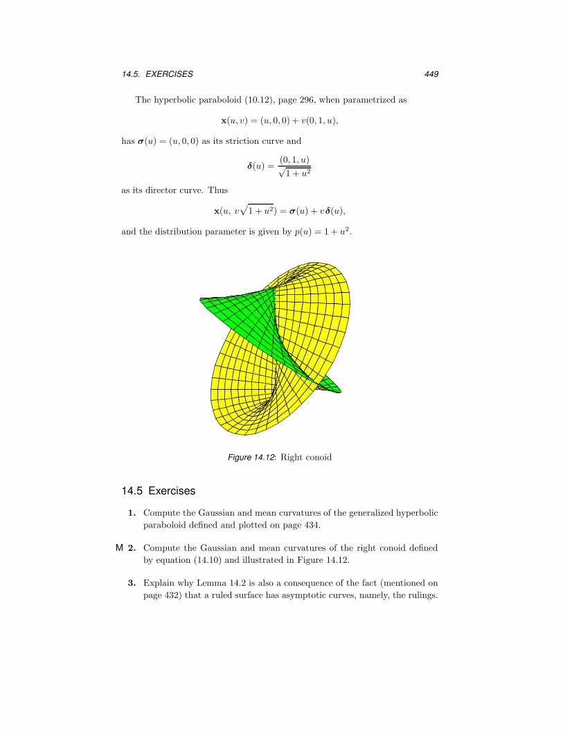
The hyperbolic paraboloid (10.12), page 296, when parametrized as
x(u, v) = (u, 0, 0) + v(0, 1, u),
has σ(u) = (u, 0, 0) as its striction curve and
δ(u) =(0, 1, u)√
1 + u2
as its director curve. Thus
x(u, v√
1 + u2) = σ(u) + vδ(u),
and the distribution parameter is given by p(u) = 1 + u2.
Figure 14.12: Right conoid
14.5 Exercises
1. Compute the Gaussian and mean curvatures of the generalized hyperbolic
paraboloid defined and plotted on page 434.
M 2. Compute the Gaussian and mean curvatures of the right conoid defined
by equation (14.10) and illustrated in Figure 14.12.
3. Explain why Lemma 14.2 is also a consequence of the fact (mentioned on
page 432) that a ruled surface has asymptotic curves, namely, the rulings.
450 CHAPTER 14. RULED SURFACES
M 4. Further to Exercise 2 of the previous chapter, describe the sets of elliptic,
hyperbolic, parabolic and planar points for the following surfaces:
(a) a cylinder over an ellipse,
(b) a cylinder over a parabola,
(c) a cylinder over a hyperbola,
(d) a cylinder over y = x3,
(e) a cone over a circle.
M 5. Compute the Gaussian and mean curvature of the patch
plueckerpolar[m, n, a](r, θ) = a(r cos θ, r sin θ, rm sin nθ
)
that generalizes plueckerpolar on page 436. Relate the case m = n = 3 to
the monkey saddle on page 304.
6. Complete the proof of Lemma 14.5 and prove Lemma 14.8.
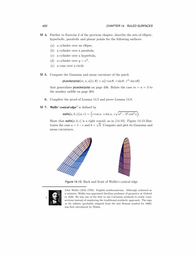
M 7. Wallis’ conical edge2 is defined by
wallis[a, b, c](u, v) =(v cosu, v sin u, c
√a2 − b2 cos2 u
).
Show that wallis[a, b, c] is a right conoid, as in (14.10). Figure 14.13 illus-
trates the case a = 1− c and b =√
3. Compute and plot its Gaussian and
mean curvatures.
Figure 14.13: Back and front of Wallis’s conical edge
2
John Wallis (1616–1703). English mathematician. Although ordained as
a minister, Wallis was appointed Savilian professor of geometry at Oxford
in 1649. He was one of the first to use Cartesian methods to study conic
sections instead of employing the traditional synthetic approach. The sign
∞ for infinity (probably adapted from the late Roman symbol for 1000)
was first introduced by Wallis.
14.5. EXERCISES 451
8. Show that the parametrization exptwist[a, c] of the expondentially twisted
helicoid described on page 563 of the next chapter is a ruled patch. Find
the rulings.
M 9. Plot the tangent developable to the twisted cubic defined on page 202.
M 10. Plot the tangent developable to the Viviani curve defined on page 207 for
the complete range −2π 6 t 6 2π (see Figure 14.10).
11. Plot the tangent developable to the bicylinder defined on page 214.
M 12. Carry out the calculations of Theorem 14.7 by computer.
M 13. Show that the normal surface to a circular helix is a helicoid. Draw the
binormal surface to a circular helix and compute its Gaussian curvature.
M 14. For any space curve α, there are other surfaces which lie between the
normal surface and the binormal surface. Consider
perpsurf[φ, α](u, v) = α(u) + v cosφN(u) + sin φB(u),
where N,B are the normal and binormal vector fields to α. Clearly,
perpsurf[0, α] is the normal surface of α, whilst perpsurf[π2, α] is its bi-
normal surface. Use perpsurf to construct several of these intermediate
surfaces for a helix.


