

Runge-Kutta and CollocationMethods
Florian Landis
Geometrical Numetric Integration – p.1
Overview
• Define Runge-Kutta methods.
• Introduce collocation methods.
• Identify collocation methods as Runge-Kutta
methods.• Find conditions to determine, of what order
collocation methods are.
Geometrical Numetric Integration – p.2
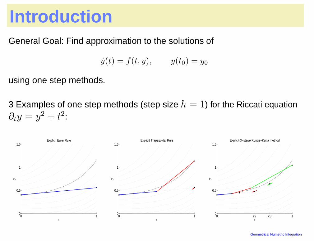
IntroductionGeneral Goal: Find approximation to the solutions of
y(t) = f(t, y), y(t0) = y0
using one step methods.
3 Examples of one step methods (step size h = 1) for the Riccati equation∂ty = y2 + t2:
0 10
0.5
1
1.5
t
y
Explicit Euler Rule
0 10
0.5
1
1.5
t
y
Explicit Trapezoidal Rule
0 c2 c3 10
0.5
1
1.5
t
y
Explicit 3−stage Runge−Kutta method
Geometrical Numetric Integration – p.3
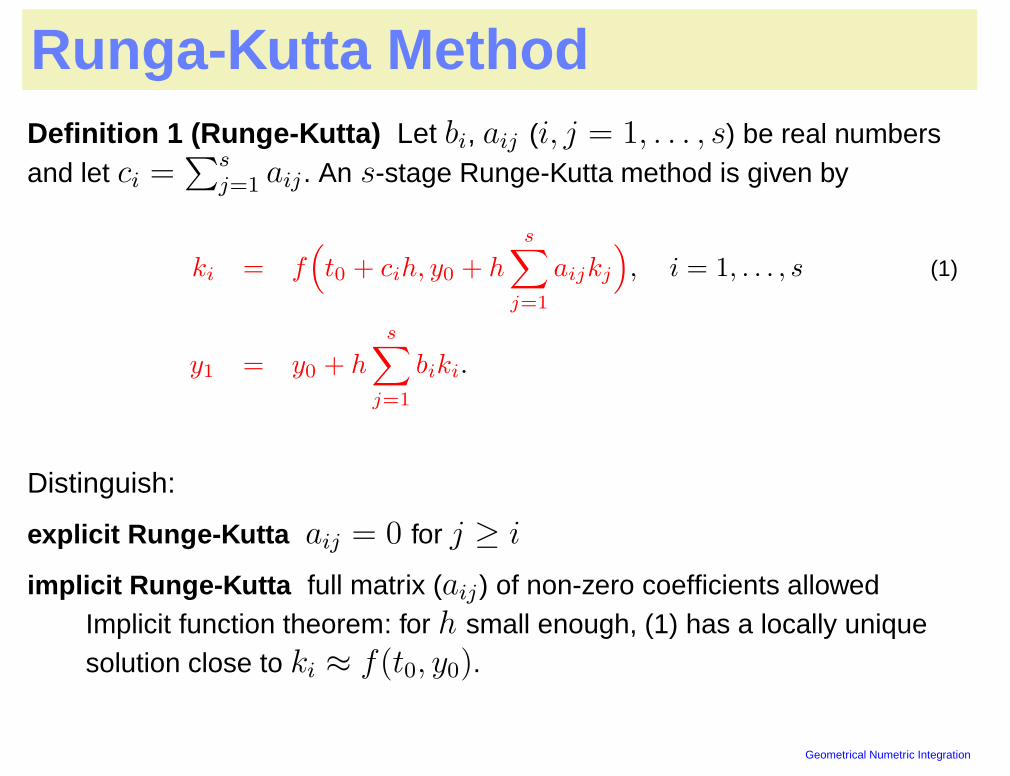
Runga-Kutta MethodDefinition 1 (Runge-Kutta) Let bi, aij (i, j = 1, . . . , s) be real numbersand let ci =
∑s
j=1 aij . An s-stage Runge-Kutta method is given by
ki = f(
t0 + cih, y0 + h
s∑
j=1
aijkj
)
, i = 1, . . . , s (1)
y1 = y0 + hs∑
j=1
biki.
Distinguish:
explicit Runge-Kutta aij = 0 for j ≥ i
implicit Runge-Kutta full matrix (aij) of non-zero coefficients allowedImplicit function theorem: for h small enough, (1) has a locally uniquesolution close to ki ≈ f(t0, y0).
Geometrical Numetric Integration – p.4
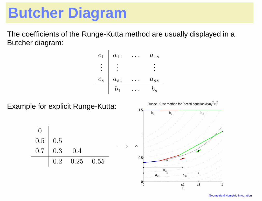
Butcher DiagramThe coefficients of the Runge-Kutta method are usually displayed in aButcher diagram:
c1 a11 . . . a1s
......
...cs as1 . . . ass
b1 . . . bs
Example for explicit Runge-Kutta:
0
0.5 0.5
0.7 0.3 0.4
0.2 0.25 0.55
−→
0 c2 c3 10
0.5
1
1.5b1 b2 b3
a21
a31 a32
t
y
Runge−Kutte method for Riccati equation ∂ty=y2+t2
Geometrical Numetric Integration – p.5
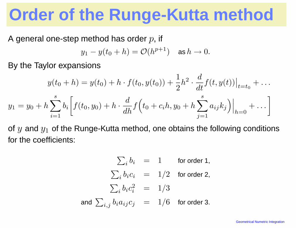
Order of the Runge-Kutta methodA general one-step method has order p, if
y1 − y(t0 + h) = O(hp+1) as h → 0.
By the Taylor expansions
y(t0 + h) = y(t0) + h · f(t0, y(t0)) +1
2h2 ·
d
dtf(t, y(t))
∣∣t=t0
+ . . .
y1 = y0 + hs∑
i=1
bi
[
f(t0, y0) + h ·d
dhf(
t0 + cih, y0 + hs∑
j=1
aijkj
)∣∣∣h=0
+ . . .
]
of y and y1 of the Runge-Kutta method, one obtains the following conditionsfor the coefficients:
∑
i bi = 1 for order 1,∑
i bici = 1/2 for order 2,∑
i bic2i = 1/3
and∑
i,j biaijcj = 1/6 for order 3.
Geometrical Numetric Integration – p.6

The Collocation MethodDefinition 2 (Collocation Method) Let c1, . . . , cs be distinct real numbers(usually 0 ≤ ci ≤ 1). The collocation polynomial u(t) is a polynomial ofdegree s satisfying
u(t0) = y0 (2)
u(t0 + cih) = f(t0 + cih, u(t0 + cih)), i = 1, . . . , s, (3)
and the numerical solution of the collocation method is defined byy1 = u(t0 + h).
0 10
0.5
1
1.5Scetch of Collocation Polynomial of degree 3y
t
u
y1
y0
c 1 c2 c3
Geometrical Numetric Integration – p.7
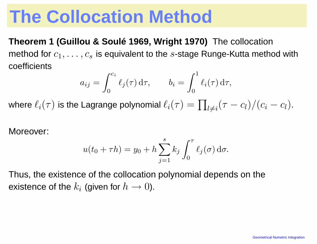
The Collocation MethodTheorem 1 (Guillou & Soulé 1969, Wright 1970) The collocationmethod for c1, . . . , cs is equivalent to the s-stage Runge-Kutta method withcoefficients
aij =
∫ ci
0
`j(τ) dτ, bi =
∫ 1
0
`i(τ) dτ,
where `i(τ) is the Lagrange polynomial `i(τ) =∏
l 6=i(τ − cl)/(ci − cl).
Moreover:
u(t0 + τh) = y0 + h
s∑
j=1
kj
∫ τ
0
`j(σ) dσ.
Thus, the existence of the collocation polynomial depends on theexistence of the ki (given for h → 0).
Geometrical Numetric Integration – p.8

Proof of Theorem 1Proof. Let u(t) be the collocation polynomial and define ki := u(t0 + cih) .By the Lagrange interpolation formula we have u(t0 + τh) =
∑s
j=1 kj · `j(τ),and by integration we get
u(t0 + cih) = y0 + hs∑
j=1
kj
∫ ci
0
`j(τ) dτ .
Inserted into the definition of the collocation polynomial
u(t0 + cih) = f(t0 + cih, u(t0 + cih)),
this gives the first formula of the Runge-Kutta equation
ki = f(
t0 + cih, y0 + hs∑
j=1
aijkj
)
.
Integration from 0 to 1 yields y1 = y0 + h∑s
j=1 biki. �
Geometrical Numetric Integration – p.9
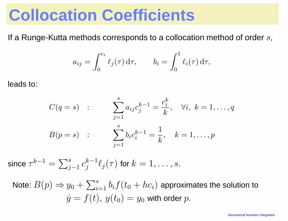
Collocation CoefficientsIf a Runge-Kutta methods corresponds to a collocation method of order s,
aij =
∫ ci
0
`j(τ) dτ, bi =
∫ 1
0
`i(τ) dτ,
leads to:
C(q = s) :s∑
j=1
aijck−1j =
cki
k, ∀i, k = 1, . . . , q
B(p = s) :s∑
j=1
bick−1i =
1
k, k = 1, . . . , p
since τ k−1 =∑s
j−1 ck−1j `j(τ) for k = 1, . . . , s.
Note: B(p) ⇒ y0 +∑s
i=1 bif(t0 + hci) approximates the solution to
y = f(t), y(t0) = y0 with order p.
Geometrical Numetric Integration – p.10
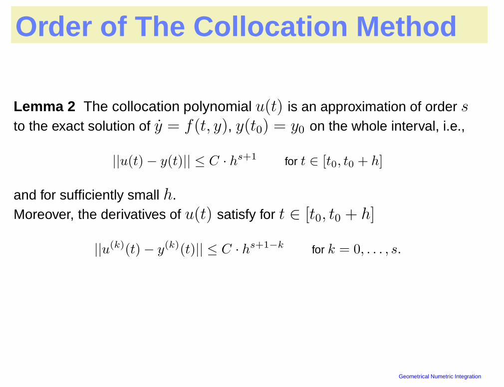
Order of The Collocation Method
Lemma 2 The collocation polynomial u(t) is an approximation of order sto the exact solution of y = f(t, y), y(t0) = y0 on the whole interval, i.e.,
||u(t) − y(t)|| ≤ C · hs+1 for t ∈ [t0, t0 + h]
and for sufficiently small h.Moreover, the derivatives of u(t) satisfy for t ∈ [t0, t0 + h]
||u(k)(t) − y(k)(t)|| ≤ C · hs+1−k for k = 0, . . . , s.
Geometrical Numetric Integration – p.11
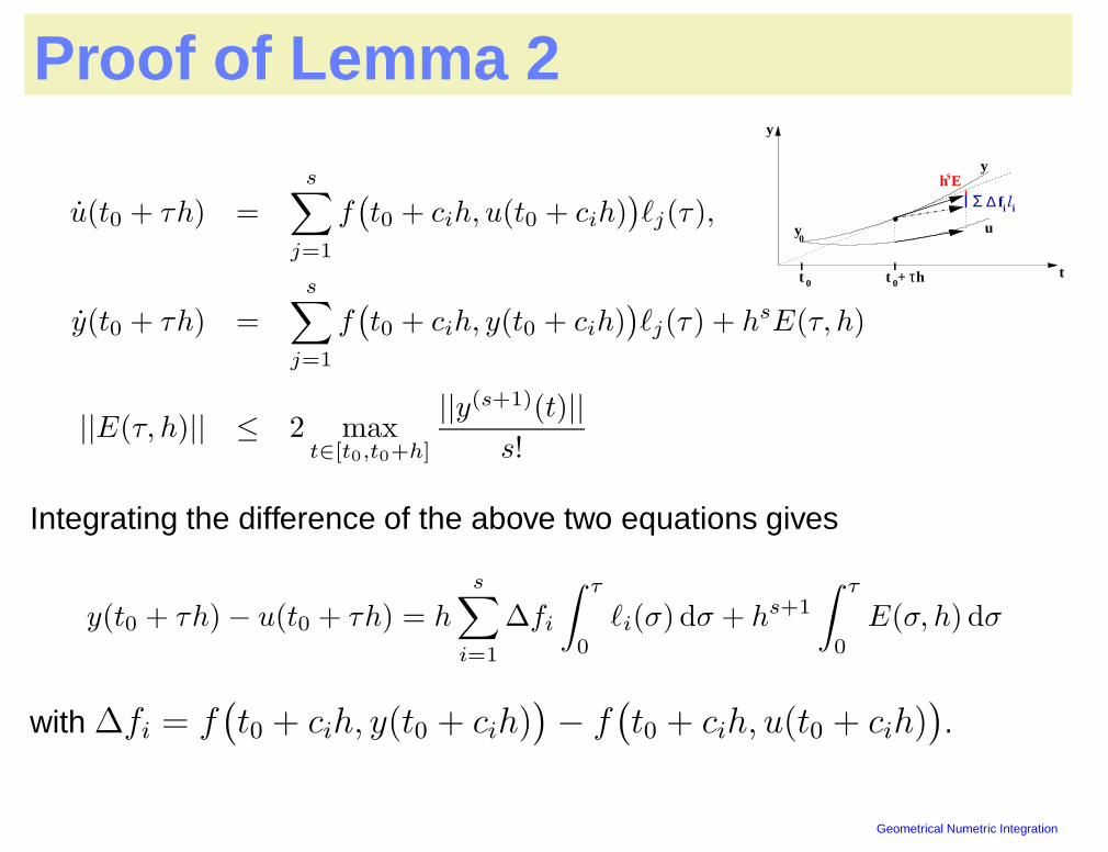
Proof of Lemma 2
u(t0 + τh) =s∑
j=1
f(t0 + cih, u(t0 + cih)
)`j(τ),
y(t0 + τh) =s∑
j=1
f(t0 + cih, y(t0 + cih)
)`j(τ) + hsE(τ, h)
||E(τ, h)|| ≤ 2 maxt∈[t0,t0+h]
||y(s+1)(t)||
s!
Integrating the difference of the above two equations gives
y(t0 + τh) − u(t0 + τh) = hs∑
i=1
∆fi
∫ τ
0
`i(σ) dσ + hs+1
∫ τ
0
E(σ, h) dσ
with ∆fi = f(t0 + cih, y(t0 + cih)
)− f
(t0 + cih, u(t0 + cih)
).
t
E
y
y0
y
u
∆ fi li
hs
tt 0 0+ τh
Σ
Geometrical Numetric Integration – p.12
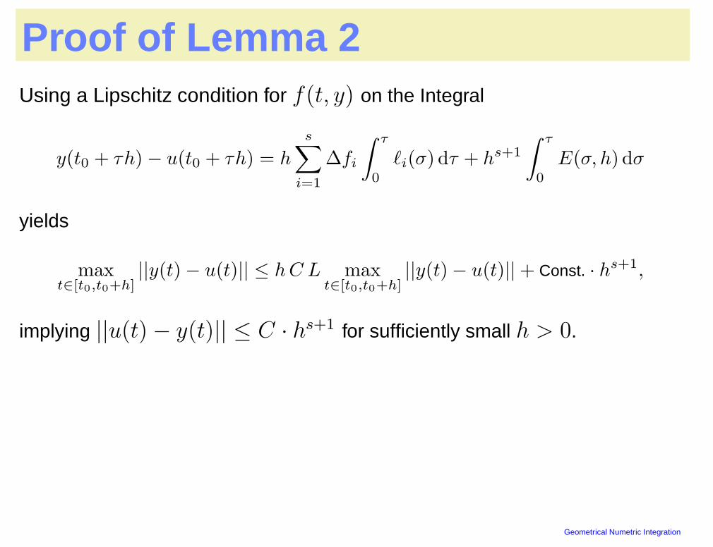
Proof of Lemma 2Using a Lipschitz condition for f(t, y) on the Integral
y(t0 + τh) − u(t0 + τh) = hs∑
i=1
∆fi
∫ τ
0
`i(σ) dτ + hs+1
∫ τ
0
E(σ, h) dσ
yields
maxt∈[t0,t0+h]
||y(t) − u(t)|| ≤ h C L maxt∈[t0,t0+h]
||y(t) − u(t)|| + Const. · hs+1,
implying ||u(t) − y(t)|| ≤ C · hs+1 for sufficiently small h > 0.
Geometrical Numetric Integration – p.13
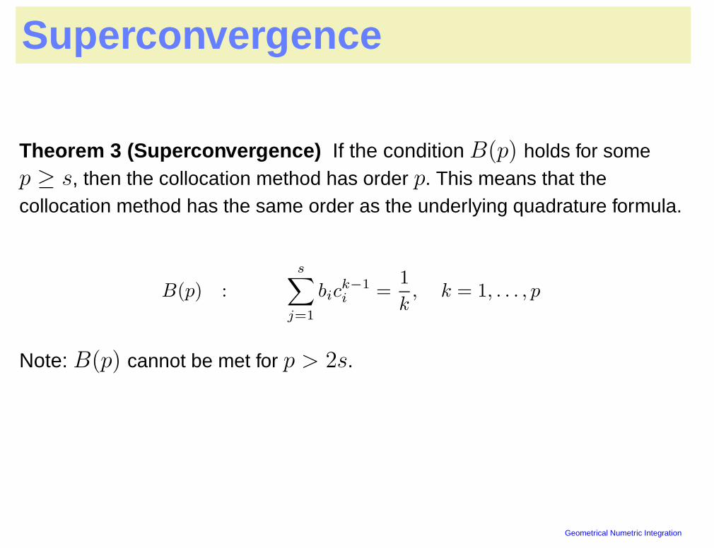
Superconvergence
Theorem 3 (Superconvergence) If the condition B(p) holds for somep ≥ s, then the collocation method has order p. This means that thecollocation method has the same order as the underlying quadrature formula.
B(p) :s∑
j=1
bick−1i =
1
k, k = 1, . . . , p
Note: B(p) cannot be met for p > 2s.
Geometrical Numetric Integration – p.14
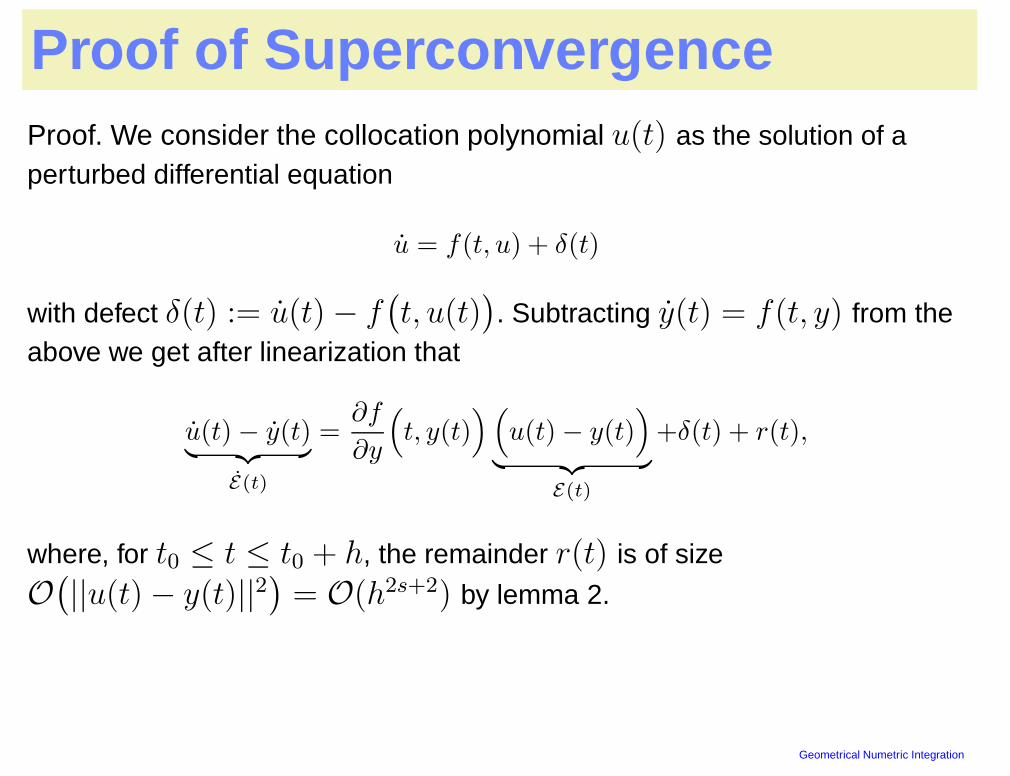
Proof of SuperconvergenceProof. We consider the collocation polynomial u(t) as the solution of aperturbed differential equation
u = f(t, u) + δ(t)
with defect δ(t) := u(t) − f(t, u(t)
). Subtracting y(t) = f(t, y) from the
above we get after linearization that
u(t) − y(t)︸ ︷︷ ︸
E(t)
=∂f
∂y
(
t, y(t)) (
u(t) − y(t))
︸ ︷︷ ︸
E(t)
+δ(t) + r(t),
where, for t0 ≤ t ≤ t0 + h, the remainder r(t) is of size
O(||u(t) − y(t)||2
)= O(h2s+2) by lemma 2.
Geometrical Numetric Integration – p.15
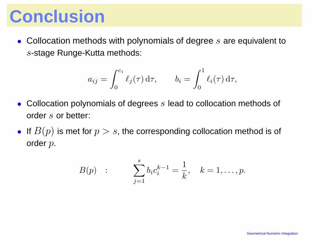
Conclusion• Collocation methods with polynomials of degree s are equivalent to
s-stage Runge-Kutta methods:
aij =
∫ ci
0
`j(τ) dτ, bi =
∫ 1
0
`i(τ) dτ,
• Collocation polynomials of degrees s lead to collocation methods oforder s or better:
• If B(p) is met for p > s, the corresponding collocation method is oforder p.
B(p) :s∑
j=1
bick−1i =
1
k, k = 1, . . . , p.
Geometrical Numetric Integration – p.16

Geometrical Numetric Integration – p.17
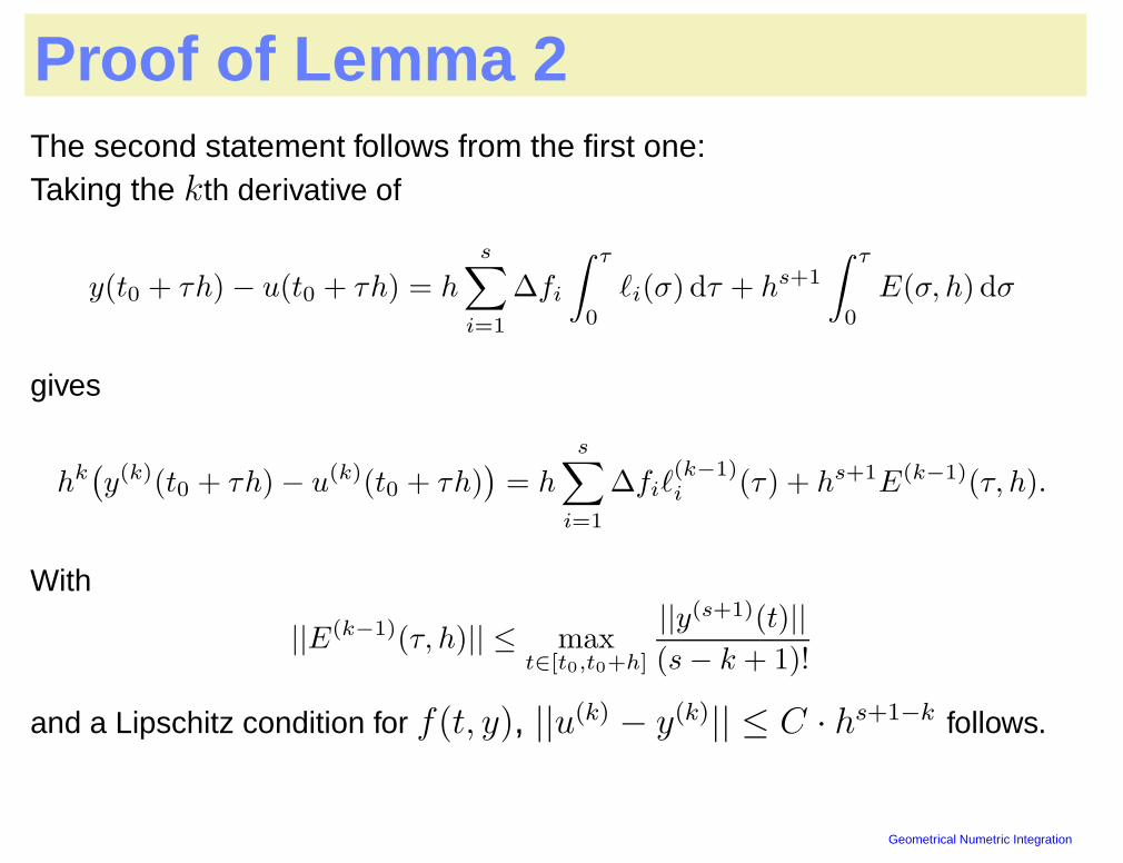
Proof of Lemma 2The second statement follows from the first one:Taking the kth derivative of
y(t0 + τh) − u(t0 + τh) = hs∑
i=1
∆fi
∫ τ
0
`i(σ) dτ + hs+1
∫ τ
0
E(σ, h) dσ
gives
hk(y(k)(t0 + τh) − u(k)(t0 + τh)
)= h
s∑
i=1
∆fi`(k−1)i (τ) + hs+1E(k−1)(τ, h).
With
||E(k−1)(τ, h)|| ≤ maxt∈[t0,t0+h]
||y(s+1)(t)||
(s − k + 1)!
and a Lipschitz condition for f(t, y), ||u(k) − y(k)|| ≤ C · hs+1−k follows.
Geometrical Numetric Integration – p.18
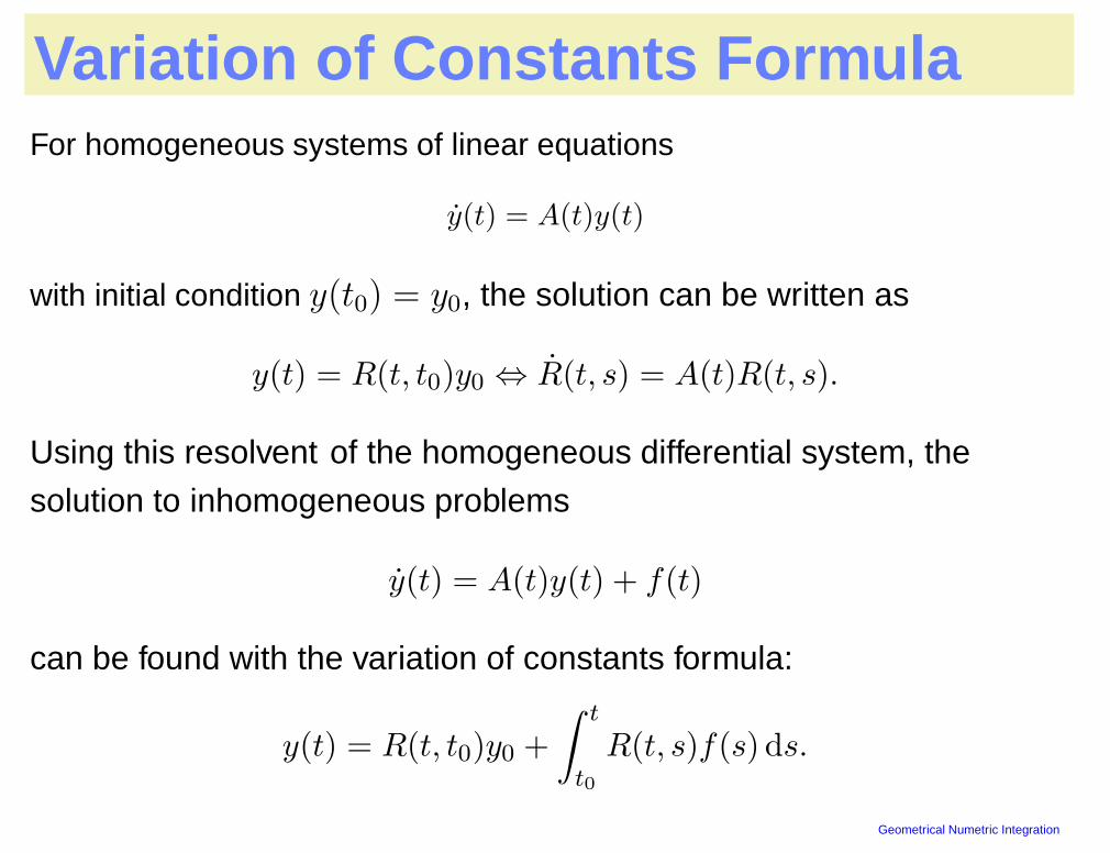
Variation of Constants FormulaFor homogeneous systems of linear equations
y(t) = A(t)y(t)
with initial condition y(t0) = y0, the solution can be written as
y(t) = R(t, t0)y0 ⇔ R(t, s) = A(t)R(t, s).
Using this resolvent of the homogeneous differential system, the
solution to inhomogeneous problems
y(t) = A(t)y(t) + f(t)
can be found with the variation of constants formula:
y(t) = R(t, t0)y0 +
∫ t
t0
R(t, s)f(s) ds.
Geometrical Numetric Integration – p.19
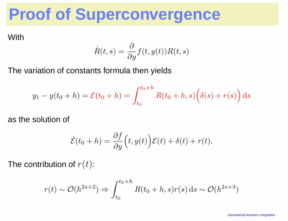
Proof of SuperconvergenceWith
R(t, s) =∂
∂yf(t, y(t))R(t, s)
The variation of constants formula then yields
y1 − y(t0 + h) = E(t0 + h) =
∫ t0+h
t0
R(t0 + h, s)(
δ(s) + r(s))
ds
as the solution of
E(t0 + h) =∂f
∂y
(
t, y(t))
E(t) + δ(t) + r(t).
The contribution of r(t):
r(t) ∼ O(h2s+2) ⇒
∫ t0+h
t0
R(t0 + h, s)r(s) ds ∼ O(h2s+3)
Geometrical Numetric Integration – p.20
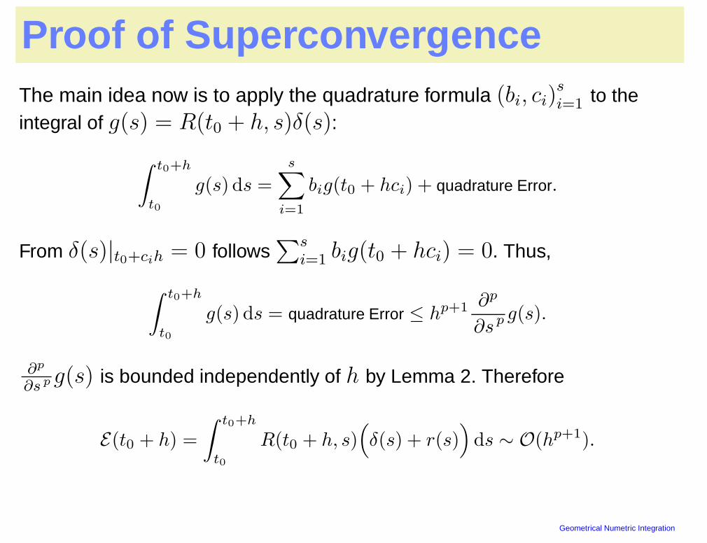
Proof of SuperconvergenceThe main idea now is to apply the quadrature formula (bi, ci)
s
i=1 to theintegral of g(s) = R(t0 + h, s)δ(s):
∫ t0+h
t0
g(s) ds =s∑
i=1
big(t0 + hci) + quadrature Error.
From δ(s)|t0+cih = 0 follows∑s
i=1 big(t0 + hci) = 0. Thus,
∫ t0+h
t0
g(s) ds = quadrature Error ≤ hp+1 ∂p
∂sp g(s).
∂p
∂s p g(s) is bounded independently of h by Lemma 2. Therefore
E(t0 + h) =
∫ t0+h
t0
R(t0 + h, s)(
δ(s) + r(s))
ds ∼ O(hp+1).
Geometrical Numetric Integration – p.21
![Third-order Composite Runge Kutta Method for Solving Fuzzy … · Adam Bashford [14], Runge Kutta of order five [15], block methods [16], and Runge-Kutta Method with Harmonic Mean](https://static.documents.pub/doc/80x56/5e2750b6a2f1ce49c1270795/third-order-composite-runge-kutta-method-for-solving-fuzzy-adam-bashford-14-runge.jpg)


