

Salem Saleh Balobaid
ID: 213203284
Deakin University
PRINCIPLES OF THERMODYNAMICS
SEM314
(2013)
LAB REPORT
Due Date
27th SEPT 2013
Experiment 1
Determination of heat capacity ratio
Objective
To determine the heat capacity ratio ⁄ for air near standard temperature and
pressure
Method
The experiment involves a two-step process. In the first step a pressurised vessel is
depressurised briefly by opening then closing a large bore valve very quickly. The gas inside
the vessel expands from to - a process that can be assumed as adiabatic and reversible
( ⁄⁄ is constant)
The volume of the gas inside the vessel is then allowed to return thermal equilibrium,
attaining a final pressure . The second step is therefore a constant volume process (P/T is
constant)
Theory
For a perfect gas,
Where = molar heat capacity at constant pressure, and
= molar heat capacity at constant volume.
For a real gas a relationship may be defined between the heat capacities, which are
dependent on the equation of state, although it is more complex than that for a perfect gas.
The heat capacity ratio may then be determined experimentally using a two-step process:
1. An adiabatic reversible expansion from the initial pressure P, to an intermediate
pressure Pi
{Ps, Volls, Ts} {Pi, Volli, Ti}
2. A return of the temperature to its original value Ts at constant volume Volli
For a reversible adiabatic expansion
From the First Law of Thermodynamics,
Therefore during the expansion process
or
At constant volume the heat capacity relates the change in temperature to the change in
internal energy
Substituting in to equation x,
Substituting in the ideal gas law and then integrating gives
(
) (
)
Now, for an ideal gas
Therefore,
(
)
Rearranging and substituting in from equation x,
During the return of the temperature to the starting value,

Thus
Rearranging gives the relationship in its required form:
Experimental Data
Observations 1 2 3
Atmospheric Pressure (absolute), Patm (N/m2)
Starting Pressure (measured), Ps(N/m2)
Starting Pressure (absolute), Pabss(N/m2)
Intermediate Pressure (measured), Pi (N/m2)
Intermediate Pressure (measured), Pabsi
(N/m2)
Final Pressure (measured), Pf (N/m2)
Final Pressure (absolute), Pabsf (N/m2)
Result and Calculation
For observation 1:
Following same calculation procedure,

for observation 2,
for observation 3,
Conclusions
In this experiment, the heat capacity ration or adiabatic index of air have been measured
three times at near standard temperature and pressure. The result obtained was quiet close
to the value expected. There were some errors came out after calculation which shows slight
difference from the actual value. This experiment allows us to understand the adiabatic
process and the steps to determine the heat capacity ratio of air.
Questions and Answers
1. Why can the initial expansion process be considered adiabatic?
An adiabatic process is a process where no thermal energy is transferred from or to
the system ( . It is possible is the system is completely isolated or is the time
taken to undergo change in the system is very negligible. Rapid change is the system
does not allow any heat to be transferred from or to the system thus creates adiabatic
process. In this experiment the pressure released from the initial state to intermediate
state so quickly that there were no chance of heat to be escaped or added from the
surroundings.
2. How well does the result obtained compare to the expected result? Give possible
reason for any difference.
The heat capacity ratio or adiabatic index of air at standard pressure and
temperature of dry air was found three different values (1.383, 1.457, and 1.451) from
three observations. The actual value of heat capacity ratio of dry air at 20oC is 1.40
(source: Wikipedia). The average value from this experiment comes up with 1.43. This
variation is mainly due to inaccuracy in measuring pressure from the apparatus.
Pressure readings were taken manually hence deviation from accuracy generated. It can
be improved by taking all those pressure values more precisely by using data logger
during the experiment.
Experiment: 2
Simple Refrigeration cycle
Objective
To determine the average thermal output and refrigeration capacity of a simple compression
refrigeration cycle;
Theory
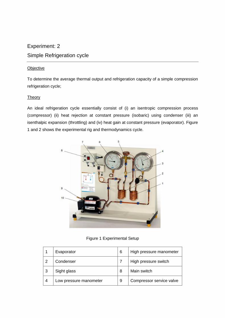
An ideal refrigeration cycle essentially consist of (i) an isentropic compression process
(compressor) (ii) heat rejection at constant pressure (isobaric) using condenser (iii) an
isenthalpic expansion (throttling) and (iv) heat gain at constant pressure (evaporator). Figure
1 and 2 shows the experimental rig and thermodynamics cycle.
Figure 1 Experimental Setup
1 Evaporator 6 High pressure manometer
2 Condenser 7 High pressure switch
3 Sight glass 8 Main switch
4 Low pressure manometer 9 Compressor service valve
5 Thermoelectric expansion valve 10 Compressor
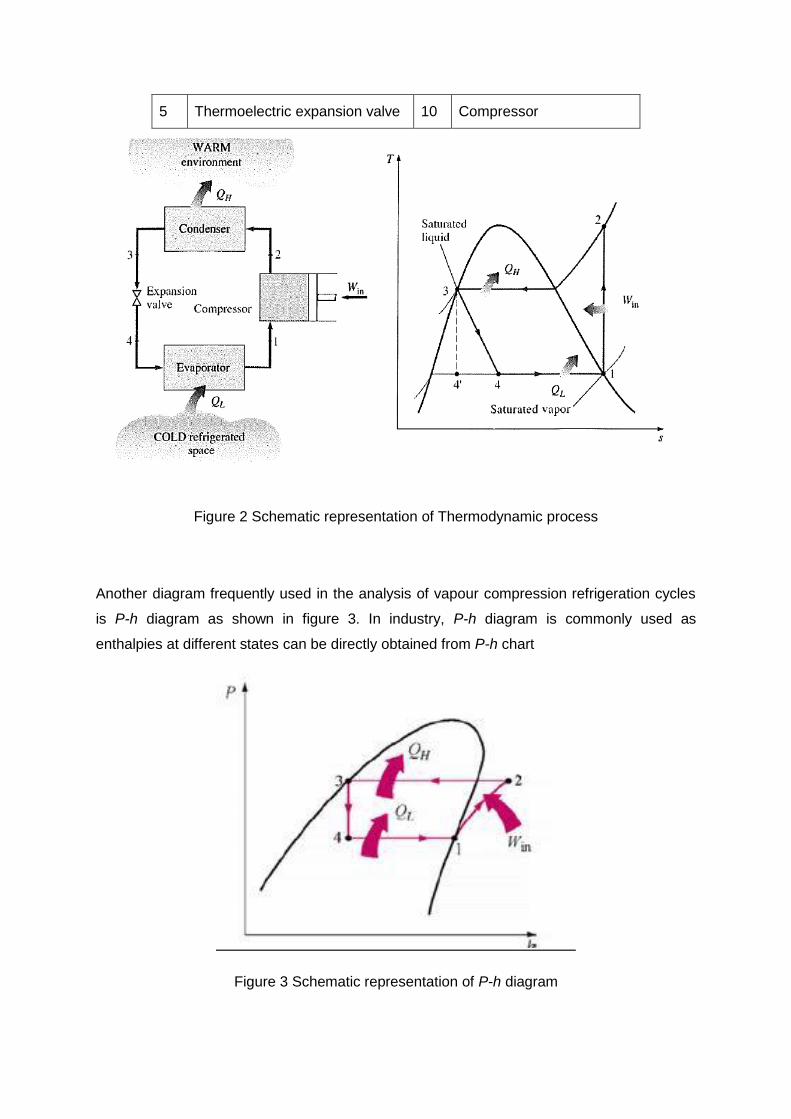
Figure 2 Schematic representation of Thermodynamic process
Another diagram frequently used in the analysis of vapour compression refrigeration cycles
is P-h diagram as shown in figure 3. In industry, P-h diagram is commonly used as
enthalpies at different states can be directly obtained from P-h chart
Figure 3 Schematic representation of P-h diagram
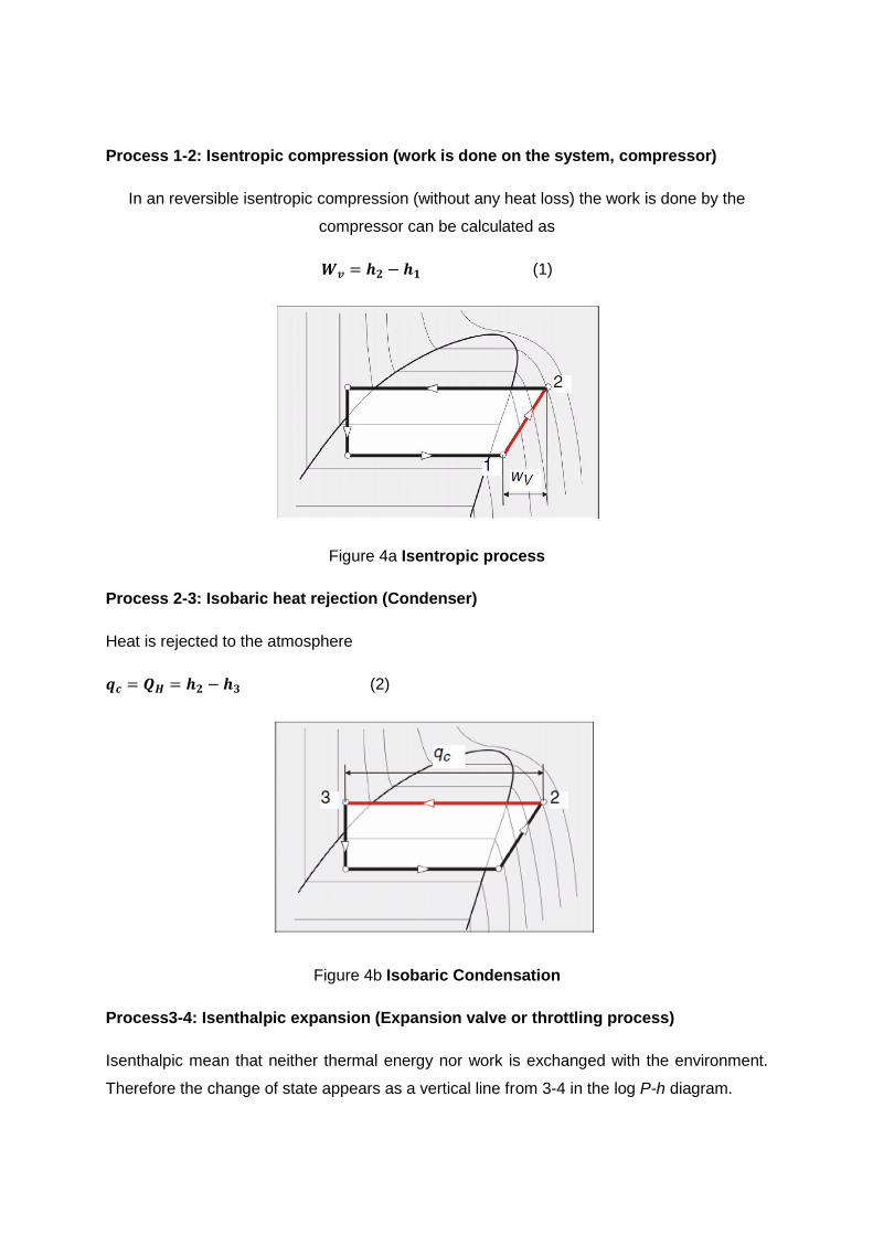
Process 1-2: Isentropic compression (work is done on the system, compressor)
In an reversible isentropic compression (without any heat loss) the work is done by the
compressor can be calculated as
(1)
Figure 4a Isentropic process
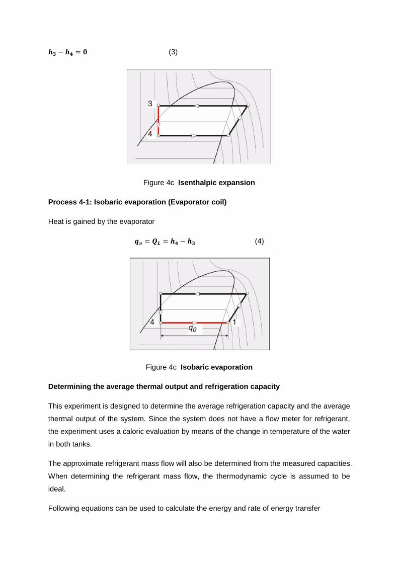
Process 2-3: Isobaric heat rejection (Condenser)
Heat is rejected to the atmosphere
(2)
Figure 4b Isobaric Condensation
Process3-4: Isenthalpic expansion (Expansion valve or throttling process)
Isenthalpic mean that neither thermal energy nor work is exchanged with the environment.
Therefore the change of state appears as a vertical line from 3-4 in the log P-h diagram.
(3)
Figure 4c Isenthalpic expansion
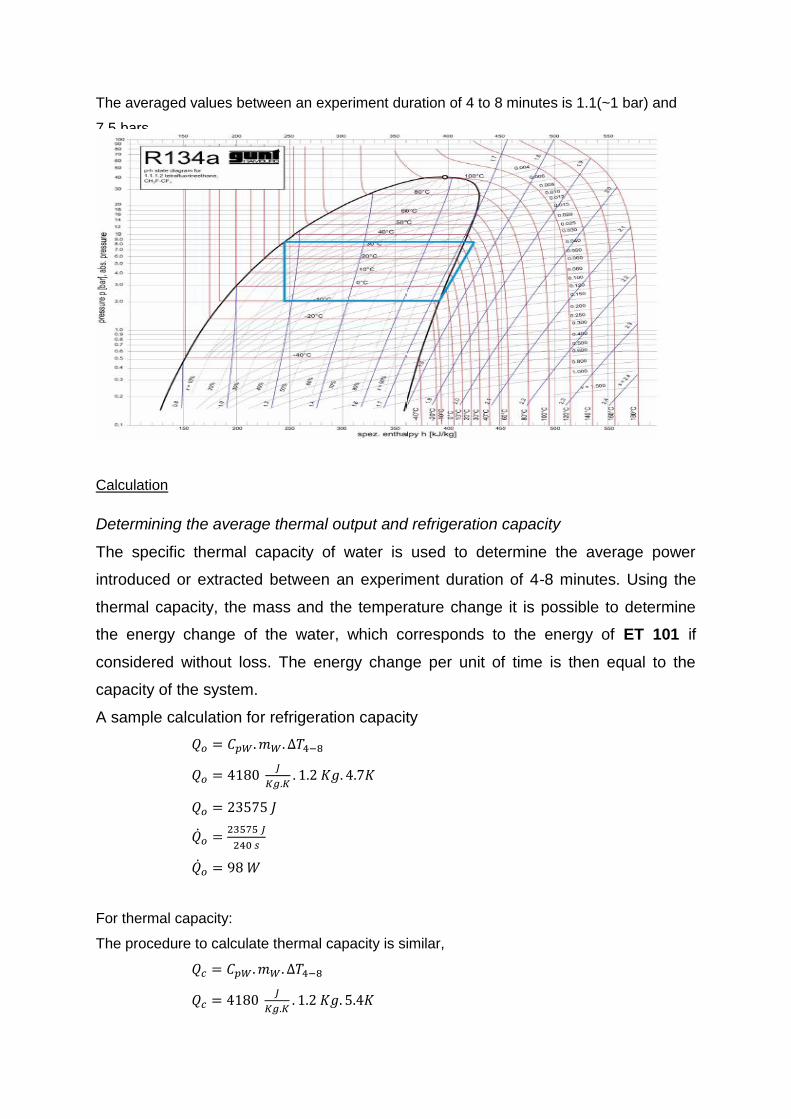
Process 4-1: Isobaric evaporation (Evaporator coil)
Heat is gained by the evaporator
(4)
Figure 4c Isobaric evaporation
Determining the average thermal output and refrigeration capacity
This experiment is designed to determine the average refrigeration capacity and the average
thermal output of the system. Since the system does not have a flow meter for refrigerant,
the experiment uses a caloric evaluation by means of the change in temperature of the water
in both tanks.
The approximate refrigerant mass flow will also be determined from the measured capacities.
When determining the refrigerant mass flow, the thermodynamic cycle is assumed to be
ideal.
Following equations can be used to calculate the energy and rate of energy transfer

(5)
(6)
Measurements
Time (min) P1 in bar P2 in bar Twc Twh
0 6.8 6.5 20.5 25
2 1 7.25 18 26
4 1.0 7.0 18.2 24.3
6 1.1 7.75 15 28
8 1.2 8.0 13.5 29.7
10 1.2 8.5 13 31
12 1.2 9.0 12 31
14 1.3 9.5 10 36
16 1.3 10.0 9 39
18 1.4 10.5 7 40
20 1.5 11.25 5 41
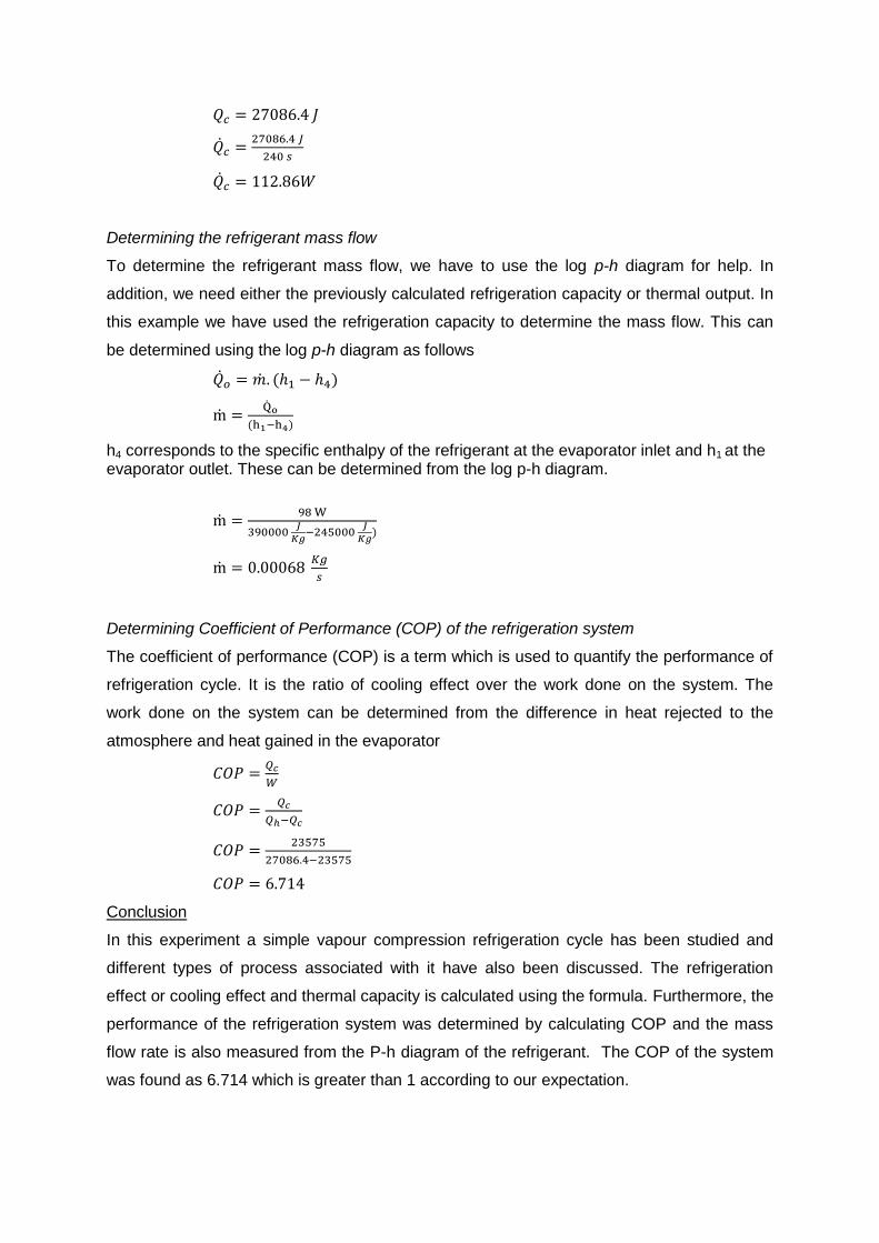
The averaged values between an experiment duration of 4 to 8 minutes is 1.1(~1 bar) and
7.5 bars.
Calculation
Determining the average thermal output and refrigeration capacity
The specific thermal capacity of water is used to determine the average power
introduced or extracted between an experiment duration of 4-8 minutes. Using the
thermal capacity, the mass and the temperature change it is possible to determine
the energy change of the water, which corresponds to the energy of ET 101 if
considered without loss. The energy change per unit of time is then equal to the
capacity of the system.
A sample calculation for refrigeration capacity
For thermal capacity:
The procedure to calculate thermal capacity is similar,
Determining the refrigerant mass flow
To determine the refrigerant mass flow, we have to use the log p-h diagram for help. In
addition, we need either the previously calculated refrigeration capacity or thermal output. In
this example we have used the refrigeration capacity to determine the mass flow. This can
be determined using the log p-h diagram as follows
h4 corresponds to the specific enthalpy of the refrigerant at the evaporator inlet and h1 at the evaporator outlet. These can be determined from the log p-h diagram.
Determining Coefficient of Performance (COP) of the refrigeration system
The coefficient of performance (COP) is a term which is used to quantify the performance of
refrigeration cycle. It is the ratio of cooling effect over the work done on the system. The
work done on the system can be determined from the difference in heat rejected to the
atmosphere and heat gained in the evaporator
Conclusion
In this experiment a simple vapour compression refrigeration cycle has been studied and
different types of process associated with it have also been discussed. The refrigeration
effect or cooling effect and thermal capacity is calculated using the formula. Furthermore, the
performance of the refrigeration system was determined by calculating COP and the mass
flow rate is also measured from the P-h diagram of the refrigerant. The COP of the system
was found as 6.714 which is greater than 1 according to our expectation.
Question and Answer
1. In general which is greater: the capacity of the condenser or the capacity of the
evaporator? Justify your answer. (hint: refer to p-h diagram of a refrigeration cycle)
The capacity of the condenser is always greater than the capacity of evaporator. When
the refrigerant is compressed, it gains some heat which comes out from the mechanical
work done on it by the compressor. After being compressed it is then cooled to the
temperature from which it starts expanding and then creating cooling effect by taking
away heat from evaporator. Therefore in the condenser it has to remove heat gained in
the evaporator as well as heat gained from the mechanical work done upon it in
compressor.
Experiment: 3
Simple heat pump
Objective
To determine the average thermal output and heating capacity of a simple heat pump;
Theory
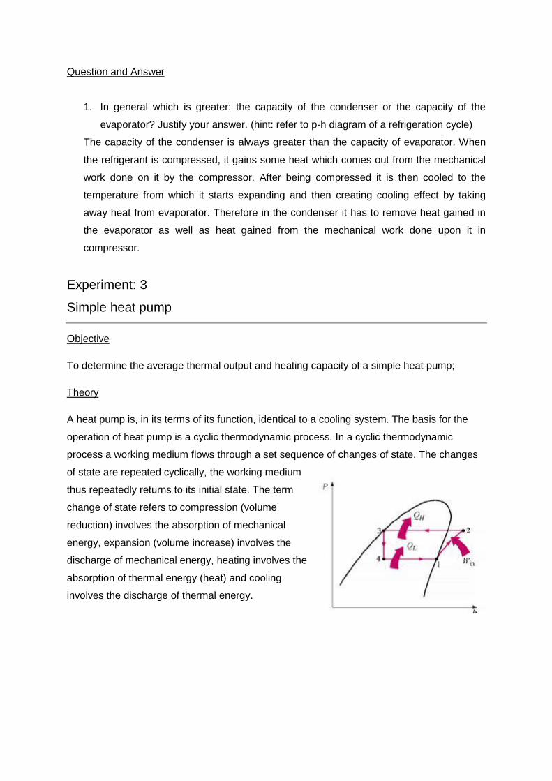
A heat pump is, in its terms of its function, identical to a cooling system. The basis for the
operation of heat pump is a cyclic thermodynamic process. In a cyclic thermodynamic
process a working medium flows through a set sequence of changes of state. The changes
of state are repeated cyclically, the working medium
thus repeatedly returns to its initial state. The term
change of state refers to compression (volume
reduction) involves the absorption of mechanical
energy, expansion (volume increase) involves the
discharge of mechanical energy, heating involves the
absorption of thermal energy (heat) and cooling
involves the discharge of thermal energy.

Figure 1 Heat pump cyclic process
Figure 2 Schematic representation of Thermodynamic process
Another diagram frequently used in the analysis of heat pump cycles is P-h diagram as
shown in figure 3. In industry, P-h diagram is commonly used as enthalpies at different
states can be directly obtained from P-h chart
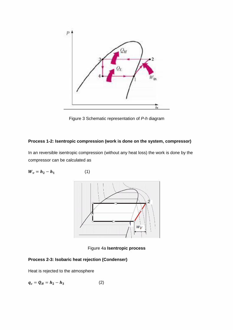
Figure 3 Schematic representation of P-h diagram
Process 1-2: Isentropic compression (work is done on the system, compressor)
In an reversible isentropic compression (without any heat loss) the work is done by the
compressor can be calculated as
(1)
Figure 4a Isentropic process
Process 2-3: Isobaric heat rejection (Condenser)
Heat is rejected to the atmosphere
(2)

Figure 4b Isobaric Condensation
Process3-4: Isenthalpic expansion (Expansion valve or throttling process)
Isenthalpic mean that neither thermal energy nor work is exchanged with the environment.
Therefore the change of state appears as a vertical line from 3-4 in the log P-h diagram.
(3)
Figure 4c Isenthalpic expansion
Process 4-1: Isobaric evaporation (Evaporator coil)
Heat is gained by the evaporator
(4)

Figure 4c Isobaric evaporation
Determining the Output coefficient (or
coefficient of performance, COP)
In order to be able to make a judgement as to the effectiveness of a heat pump, an output
coefficient is used. This corresponds to the efficiency of thermal power plants and is
determined from the relationship of benefit to work. The benefit comprises the heat flow
discharged, the work the power input Pin or the mechanical energy expended.
Contrary to the efficiency of other machines and systems, the output coefficient is in general
larger than 1. The output coefficient can therefore not be termed efficiency.
The quantities of energy converted in the cyclic process can be taken directly from the p-h
diagram as differences in the enthalpies. Thus the output coefficient for the ideal process
can be derived in a very straight forward manner
(5)
Obviously this equation goes for an ideal cycle but in actual case the process slightly differ.
For the real process with suction gas superheating and liquid supercooling the following
applies
(6)
The output coefficient can also be calculated from the actual amount of heat drawn off from
the condenser using the water circuit and the actual power input by the compressor.
Here all the losses due to radiation, heat conduction friction, etc. are also taken into account.

The benefit, that is the heat flow, is calculated from the flow of the water, the temperature
difference between the inlet and the outlet, and the specific heat capacity of water.
(7)
The lower the temperature differences between the absorption side and the suction side, the
larger the output coefficient.
Measurements
Time (min) 1 2 3 4 5
T1 in oC 12 18.5 12.1 11.4 11.7
T2 in oC 66.8 66 66.4 66.8 67.1
T3 in oC 37.6 37.4 37.6 38.2 37.7
T4 in oC 6.4 6.4 6.5 6.5 6.5
T5 in oC 33.6 33.4 33.7 33.8 33.7
T6 in oC 52.3 52.2 52.4 52.3 52.4
F1 in ltr/min 20.4 20.44 18.9 19.5 19.3
F2 in ltr/hr 20 20 20 20 20
Pel in W 213 213 213 213 213
P1/4 in bar 3.43 3.44 3.38 3.38 3.44
P2/3 in bar 14.78 14.92 14.64 14.76 14.86
h1 in kJ/kg 402.7 402.3 402.4 402.8 402.3
h2 in kJ/kg 442.4 441.6 442.0 447.8 441.8
h3 in kJ/kg 254 253.7 254 254.1 254
h4 in kJ/kg 254 253.7 254 254.1 254
Calculation

Determining the ideal and real output coefficient
Here the output coefficient is determined from the differences in the enthalpies on the log p-h
diagram. To do this the cyclic process must be plotted on the log p-h diagram.
The pressures read from observation 1 at the inlet and outlet of the compressor are now
plotted on the p-h diagram
P1/4=3.43+1 bar abs. =4.43 bar abs
P2/3=14.78+1 bar abs. =15.78 bar abs
Enthalpy values
h1 = 405.8 kJ/kg
h2 = 432 kJ/kg
h3 = h4= 217.2 kJ/kg
Compressor compression ratio
The output coefficient for the ideal cyclic process can now be calculated using the
differences in the enthalpies.

To determine the output coefficient for the real cyclic process, the cyclic process is plotted
on the p-h diagram taking the temperatures into account.
T1 = 12 oC
T2 = 66 oC
T3 = 37.6 oC
T4 = 6.4 oC
Enthalpy values:
h1* = 402.7 kJ/kg
h2* = 442.4 kJ/kg
h3* = h4
*= 254 kJ/kg
The output coefficient for the real cyclic process then has the following value
Experimental Determination of the Actual Output Coefficient
The actual output coefficient is calculated from the amount of heat extracted from the
condenser using the hot water circuit and the power input at the compressor. Here all the
losses due to radiation, heat conduction, friction, etc. are also taken into account.

The benefit, that is the heat flow, is calculated from the water flow rate, the temperature
difference between the inlet and outlet and the specific heat capacity of the water (cp =
4.19kJ/kg K).
= Flow rate in m3/s =
m3/s =5.67X10⁻⁶ m3/s
= Density in Kg/m3 = 996 Kg/m3
= Compressor output in kW = 0.213 kW
Conclusion
In this experiment a heat pump system has been thoroughly studied and the output
coefficient measured with different method. The theoretical performance numbers obtained
from the enthalpies are always slightly higher than those determined from the measured
output. This is because of the thermal output power dissipated through the compressor
housing. This heat dissipation results in removal of heat from the hot gas before the
compressor outlet. The actual output coefficient is considerably lower than the ideal/real
output coefficient due to heat losses resulting from radiation and conduction.
The output coefficient for a heat pump is dependent on the temperature gradients between
the hot medium on the hot side and the heat source on the cold side. The higher this
temperature difference, the lower the output coefficient. This effect is comparable with the
behaviour of a normal pump: the higher the pump head, the lower the capacity.

Experiment: 4
Methods of pressure and temperature measurement
Objective
To familiarize with different pressure and temperature measurement
Theory
There are various method available to measure pressure and temperature In this experiment
pressure measurement are to be carried out on a U-tube manometer, an inclined U-tube
manometer and a Bourdon gauge for positive and negative applied pressures. Temperature
measurements are to carried out using a thermocouple, resistance thermometer and a
thermistor (NTC). The temperature of water undergoing a phase change will be measure
using these measurement device mentioned above and compared. The experimental
devices are shown below:

Figure 1 Pressure measurement setup
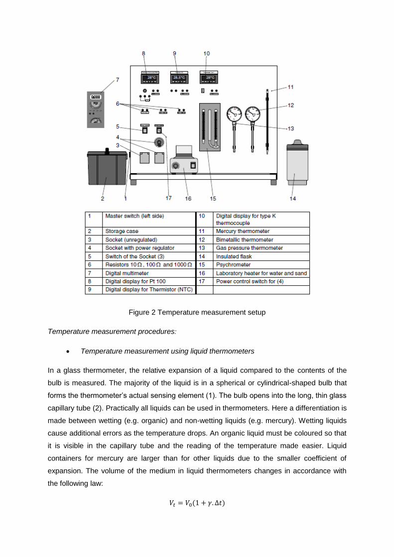
Figure 2 Temperature measurement setup
Temperature measurement procedures:
Temperature measurement using liquid thermometers
In a glass thermometer, the relative expansion of a liquid compared to the contents of the
bulb is measured. The majority of the liquid is in a spherical or cylindrical-shaped bulb that
forms the thermometer’s actual sensing element (1). The bulb opens into the long, thin glass
capillary tube (2). Practically all liquids can be used in thermometers. Here a differentiation is
made between wetting (e.g. organic) and non-wetting liquids (e.g. mercury). Wetting liquids
cause additional errors as the temperature drops. An organic liquid must be coloured so that
it is visible in the capillary tube and the reading of the temperature made easier. Liquid
containers for mercury are larger than for other liquids due to the smaller coefficient of
expansion. The volume of the medium in liquid thermometers changes in accordance with
the following law:
Vt Volume at Temperature t
V0 Volume at 0°C
Coefficient of linear expansion in 1/K
Difference in temperature from °C to K
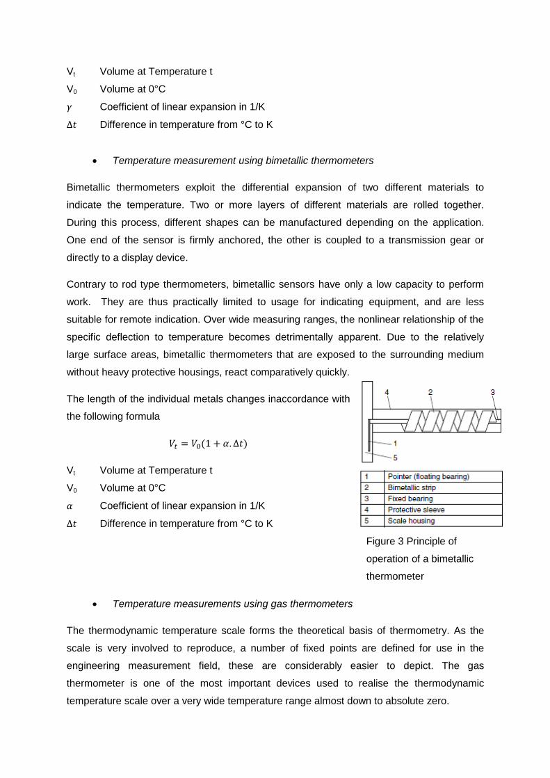
Temperature measurement using bimetallic thermometers
Bimetallic thermometers exploit the differential expansion of two different materials to
indicate the temperature. Two or more layers of different materials are rolled together.
During this process, different shapes can be manufactured depending on the application.
One end of the sensor is firmly anchored, the other is coupled to a transmission gear or
directly to a display device.
Contrary to rod type thermometers, bimetallic sensors have only a low capacity to perform
work. They are thus practically limited to usage for indicating equipment, and are less
suitable for remote indication. Over wide measuring ranges, the nonlinear relationship of the
specific deflection to temperature becomes detrimentally apparent. Due to the relatively
large surface areas, bimetallic thermometers that are exposed to the surrounding medium
without heavy protective housings, react comparatively quickly.
The length of the individual metals changes inaccordance with
the following formula
Vt Volume at Temperature t
V0 Volume at 0°C
Coefficient of linear expansion in 1/K
Difference in temperature from °C to K
Figure 3 Principle of
operation of a bimetallic
thermometer
Temperature measurements using gas thermometers
The thermodynamic temperature scale forms the theoretical basis of thermometry. As the
scale is very involved to reproduce, a number of fixed points are defined for use in the
engineering measurement field, these are considerably easier to depict. The gas
thermometer is one of the most important devices used to realise the thermodynamic
temperature scale over a very wide temperature range almost down to absolute zero.

Using this method, the change in the pressure or volume of a gas is measured as a function
of temperature in accordance with the ideal gas equation:
Here the mass m and the gas constant R are constant. All approximately ideal gases can be
used (helium, nitrogen, argon). The lowest measurable temperature is just above the critical
point of the respective charge gas (nitrogen -147°C).
The following relationship exists between the gas states at two different temperatures:
p Pressure in N/mm2
V Volume in m3
T Temperature in K
Temperature measurement using temperature measuring strips
Alongside the classic temperature measuring equipment described, which can be classified
in the mechanical contact thermometer category, there is a series of further methods that are
based on totally different physical or chemical effects. They mostly have serious
disadvantages, which is why they have not become commonly adopted in practice, but are
only used in very specific applications. One type is temperature indicating films that change
colour from light to dark at a specific temperature as a result of a chemical reaction. A heat
sensitive layer is vapour deposited on small self-adhesive pieces of plastic. The colour
change is irreversible. The error on the indication is between 1% and 2% of the printed
value. These films are suitable for a measuring range from 29°C to 290°C.
Temperature measurement using resistor thermometers
The electrical resistance of the majority of materials varies significantly with temperature.
This effect, often regarded as a problem in other areas, is exploited here for a temperature
measuring principle. The cause of this temperature dependency in metallic conductors is the
unattached bonding electrons in the metal lattice: at the temperature drops, the electrical
resistance also drops. In semiconductors there is normally a lack of conduction electrons. It
only through the addition of thermal energy (temperature increase) that electrons for the
conduction of current become free: the electrical resistance drops with increasing
temperature.
Contrary to thermocouples, using which only temperature differences compared to a known
temperature can be measured, the absolute temperature can be determined using resistive
sensor elements. Resistive sensor elements require an auxiliary power supply that is often
not used in thermocouple circuits. The measuring range of resistive sensor elements is
limited, particularly at high temperatures, the linearity of the temperature characteristic is in
some circumstances poor, depending on the material used for the sensor.
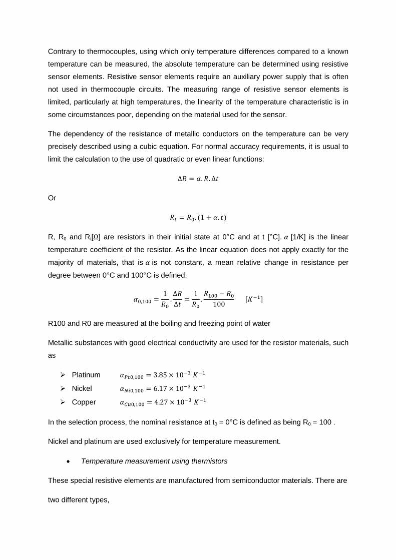
The dependency of the resistance of metallic conductors on the temperature can be very
precisely described using a cubic equation. For normal accuracy requirements, it is usual to
limit the calculation to the use of quadratic or even linear functions:
Or
R, R0 and Rt[ ] are resistors in their initial state at 0°C and at t [°C]. [1/K] is the linear
temperature coefficient of the resistor. As the linear equation does not apply exactly for the
majority of materials, that is is not constant, a mean relative change in resistance per
degree between 0°C and 100°C is defined:
R100 and R0 are measured at the boiling and freezing point of water
Metallic substances with good electrical conductivity are used for the resistor materials, such
as
Platinum
Nickel
Copper
In the selection process, the nominal resistance at t0 = 0°C is defined as being R0 = 100 .
Nickel and platinum are used exclusively for temperature measurement.
Temperature measurement using thermistors
These special resistive elements are manufactured from semiconductor materials. There are
two different types,

• NTC thermistors
• PTC thermistors.
Thermistors or NTC (negative temperature coefficient) resistors are conductive materials
that conduct current more effectively at high temperatures than at low temperatures. This
means that as the temperature increases, their electrical resistance falls. They have a
negative temperature coefficient. The opposite of thermistors are posistors (PTC resistors),
which conduct better at lower temperatures and have a positive temperature coefficient.
All semiconductor elements are ideal insulators at very low temperatures. Their increase in
conductivity is described approximately by the following law:
(
) ⇔
(
)
RT Resistance in at absolute temperature T
RN Resistance in at nominal temperature
T Operating temperature
TN Nominal temperature, normaly 25°C (298,16 K)
b Material constant 2000 to 6000 K
The material constant b and the nominal resistance are specified by the manufacturer in the
data sheet.
The normal operating range is between -80°C and +250°C.
Temperature measurement using thermocouples
The technical exploitation of the thermoelectric effect for temperature measurement began
with Seebeck and Peltier. The development and testing of new materials for thermocouples
is still not complete.
In general, any combination of two conductor materials can be utilised to manufacture a
thermocouple.
The sensitivity of the thermocouple is the algebraic sum of the thermal electromotive forces
of the two conductors. The sensitivity is very high if the thermal electromotive forces are very
different. If two different materials are welded into a thermocouple and this joint is heated, an
electromotive force (e.m.f.) is generated. With the aid of the e.m.f. the temperature becomes
a measured parameter.
The following thermocouples are standardised in terms of their e.m.f. and their tolerance:
Iron constantan (Fe-CuNi) code letter "J" up to 750°C
Copper constantan (Cu-CuNi) code letter "T" up to 350°C
Nickel-chromium nickel (NiCr-Ni) code letter "K" up to 1200°C
Nickel-chromium constantan (NiCr-CuNi) code letter "E" up to 900°C
Nicrosil nisil (NiCrSi-NiSi) code letter "N" up to 1200°C
Platinum-rhodium platinum (Pt10Rh-Pt) code letter "S" up to 1600°C
Platinum-rhodium platinum (Pt13Rh-Pt) code letter "R" up to 1600°C
Platinum-rhodium platinum (Pt30Rh-Pt6Rh) code letter "B" up to 1700°C
Experimental data
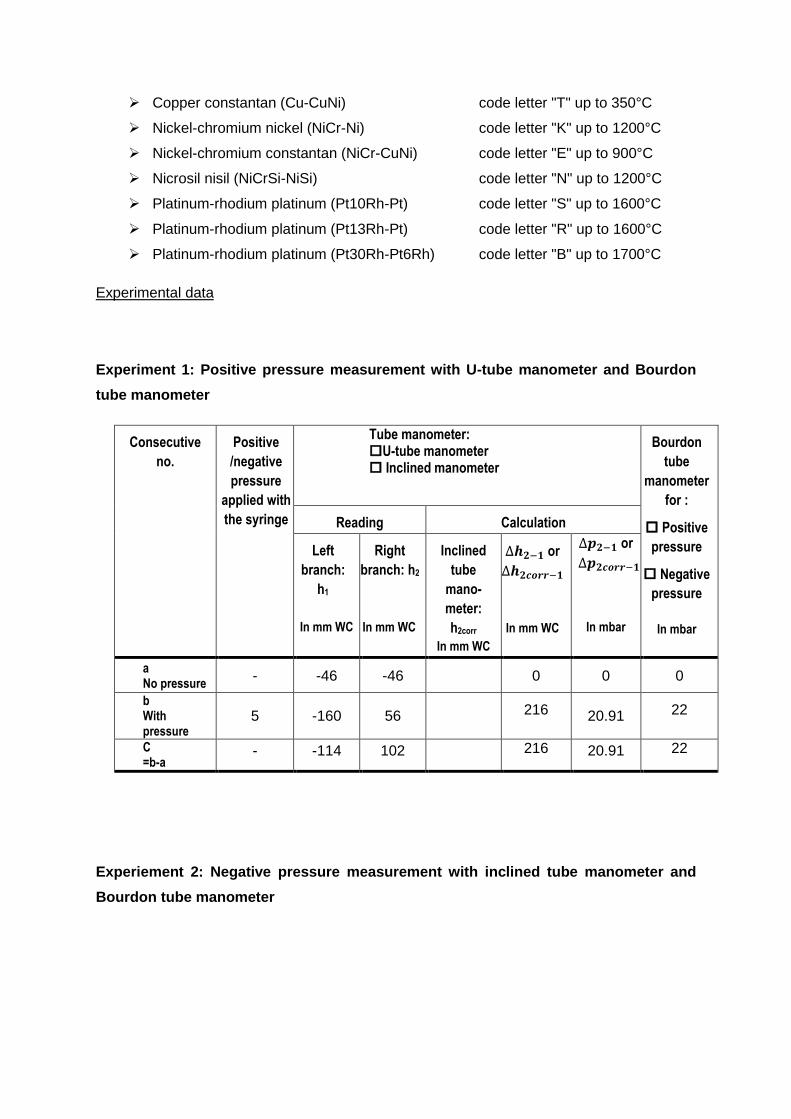
Experiment 1: Positive pressure measurement with U-tube manometer and Bourdon
tube manometer
Consecutive
no.
Positive
/negative
pressure
applied with
the syringe
Tube manometer: U-tube manometer Inclined manometer
Bourdon
tube
manometer
for :
Positive
pressure
Negative
pressure
In mbar
Reading Calculation
Left
branch:
h1
In mm WC
Right
branch: h2
In mm WC
Inclined
tube
mano-
meter:
h2corr
In mm WC
or
In mm WC
or
In mbar
a No pressure
- -46 -46 0 0 0
b With pressure
5 -160 56 216 20.91 22
C =b-a
- -114 102 216 20.91 22
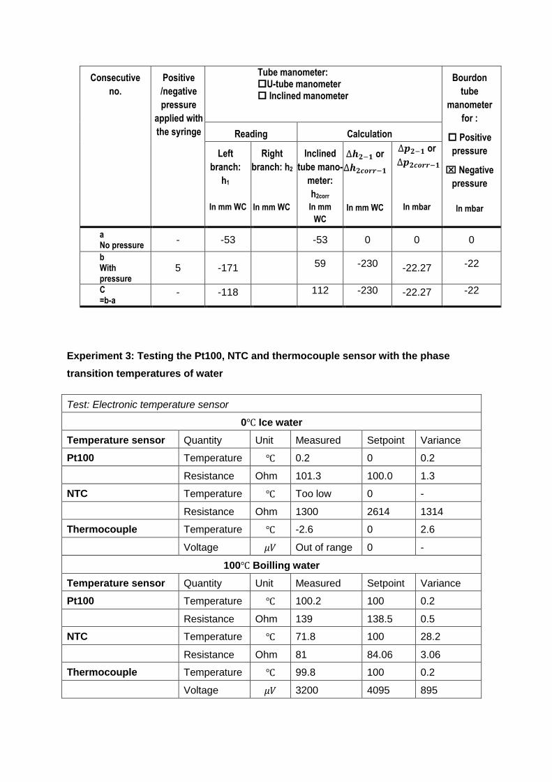
Experiement 2: Negative pressure measurement with inclined tube manometer and
Bourdon tube manometer
Consecutive
no.
Positive
/negative
pressure
applied with
the syringe
Tube manometer: U-tube manometer Inclined manometer
Bourdon
tube
manometer
for :
Positive
pressure
Negative
pressure
In mbar
Reading Calculation
Left
branch:
h1
In mm WC
Right
branch: h2
In mm WC
Inclined
tube mano-
meter:
h2corr
In mm
WC
or
In mm WC
or
In mbar
a No pressure
- -53 -53 0 0 0
b With pressure
5 -171 59 -230 -22.27 -22
C =b-a
- -118 112 -230 -22.27 -22
Experiment 3: Testing the Pt100, NTC and thermocouple sensor with the phase
transition temperatures of water
Test: Electronic temperature sensor
0 Ice water
Temperature sensor Quantity Unit Measured Setpoint Variance
Pt100 Temperature 0.2 0 0.2
Resistance Ohm 101.3 100.0 1.3
NTC Temperature Too low 0 -
Resistance Ohm 1300 2614 1314
Thermocouple Temperature -2.6 0 2.6
Voltage Out of range 0 -
100 Boilling water
Temperature sensor Quantity Unit Measured Setpoint Variance
Pt100 Temperature 100.2 100 0.2
Resistance Ohm 139 138.5 0.5
NTC Temperature 71.8 100 28.2
Resistance Ohm 81 84.06 3.06
Thermocouple Temperature 99.8 100 0.2
Voltage 3200 4095 895
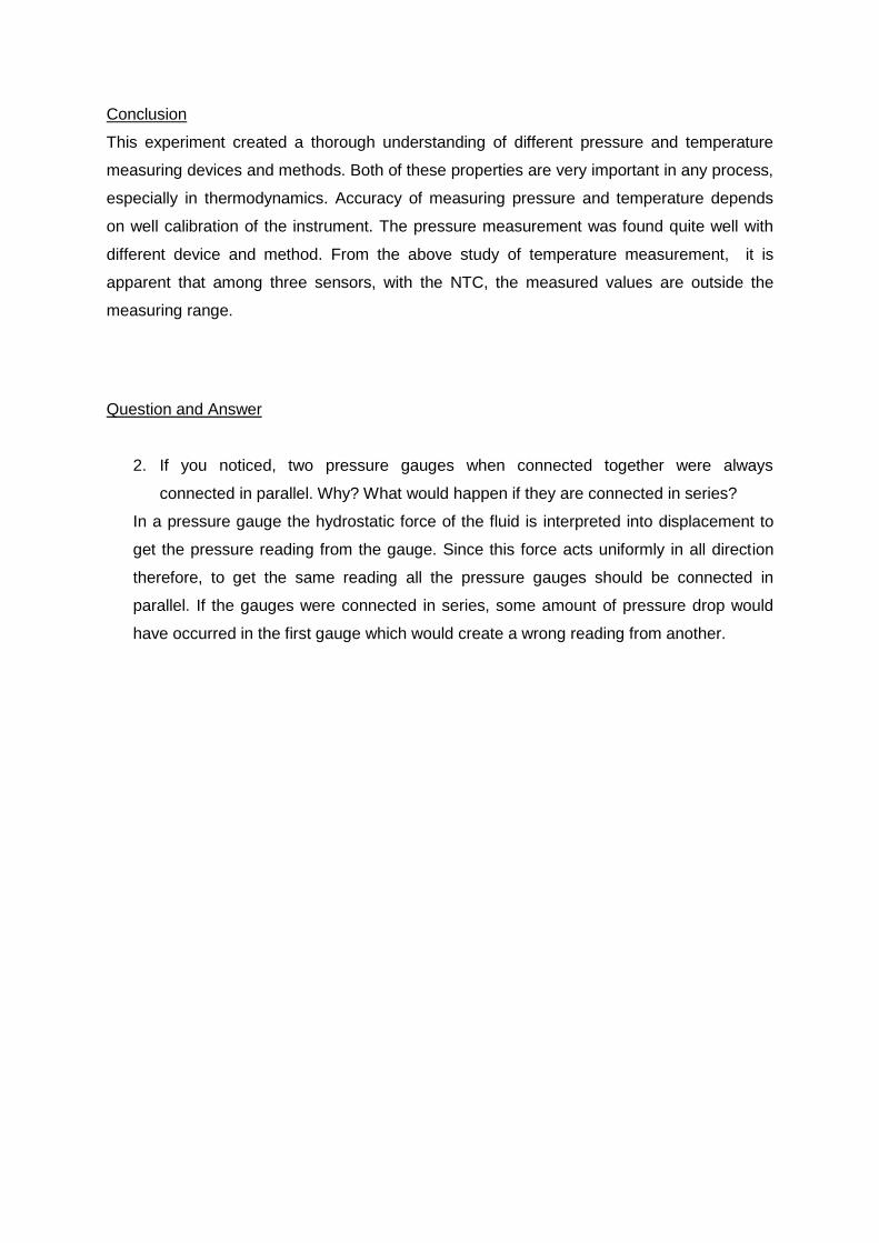
Conclusion
This experiment created a thorough understanding of different pressure and temperature
measuring devices and methods. Both of these properties are very important in any process,
especially in thermodynamics. Accuracy of measuring pressure and temperature depends
on well calibration of the instrument. The pressure measurement was found quite well with
different device and method. From the above study of temperature measurement, it is
apparent that among three sensors, with the NTC, the measured values are outside the
measuring range.
Question and Answer
2. If you noticed, two pressure gauges when connected together were always
connected in parallel. Why? What would happen if they are connected in series?
In a pressure gauge the hydrostatic force of the fluid is interpreted into displacement to
get the pressure reading from the gauge. Since this force acts uniformly in all direction
therefore, to get the same reading all the pressure gauges should be connected in
parallel. If the gauges were connected in series, some amount of pressure drop would
have occurred in the first gauge which would create a wrong reading from another.


