

1
Copyright © 2012 Quintiles
Sample Size Estimation for Observational Studies
7 November 2012
Eric Gemmen, MA
Mark Nixon, PhD
Dr. Pablo Mallaina
Andrew Burgess, BSc
2
Background and Motivation
• Unlike randomized control trials (RCTs), observational studies and patient registries typically address objectives rather than test specific hypotheses.
> Nevertheless, estimation of sample size is an important part of the planning
process.
> A minimum sample size is required to ensure:
- adequate exploration of the objectives
- ensure suff icient generalisability
• Sample size estimation for observational studies is often complex
> Subgroup analyses and modelling are to be expected in observational studies
- methods require more assumptions and larger sample sizes.
• Analysis follows design
2
3
Landscape (not necessarily unique to observational studies)
Studies with an observational unit other than the patient
Patient-years
Site/provider
Single-cohort studies
Outcome comparisons against historical comparator
Outcome comparisons w here patients serve as their ow n control (i.e., historical control, paired responses)
No comparison
Multiple comparison adjustments to support:
comparisons betw een multiple study sites or multiple patient types
comparisons using multiple interim/intermediate analyses (“refreshes of the data”)
4
Objective
To explore sample size estimations performed for a variety
of observational studies with an array of challenges and
objectives:
• Missing Data
• Selection Bias
• Unknown Enrollment Distributions
• Time-to-Event
• Precision around Point Estimate
• Need for Generalisability of Results
3
5
Sample Size Estimation in Anticipation of Missing Data, Selection Bias and Unknown Enrollment Distributions Eric Gemmen, MA
6
• Missing data is the norm in observational studies.
• Covariate-adjusted analyses use complete data only
• Example:
> Required sample size = 300
> Expect 5% of data randomly missing from 3 covariates
> Complete data in 100*0.95^3 = 86% of patients
> Corrected sample size is 300 / 0.86 = 350
• This approach is valid for complete-case analysis as well as multiple imputation.
Missing Data
4
7
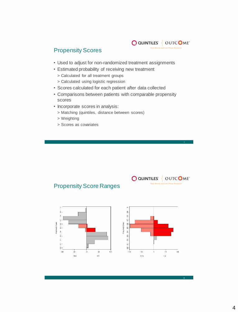
• Used to adjust for non-randomized treatment assignments
• Estimated probability of receiving new treatment
> Calculated for all treatment groups
> Calculated using logistic regression
• Scores calculated for each patient after data collected
• Comparisons between patients with comparable propensity
scores
• Incorporate scores in analysis:
> Matching (quintiles, distance between scores)
> Weighting
> Scores as covariates
Propensity Scores
8
Propensity Score Ranges
5
9
• Observational study comparing two treatments (new vs.
standard) for rheumatoid arthritis.
• Primary endpoint is change in the DAS28-ESR score at six
months.
• If this were a randomized trial, the sample size required per treatment group would be 448 (alpha = 0.05, 2-sided test,
power = 80%).
• Sample size increased to 560, assuming 80% propensity score
overlap.
Propensity Score Example
10
• Long-term longitudinal oncology study of treatment response and its association with genomic variants
• Real-world personalized medicine study with ‘standard-of-care’ treatments
• Initially, treatment patterns and distribution of genomic variants largely unknown
• Also, uncertain estimates for treatment response and dropout rates in initial
sample size calculations
• Plan to re-estimate sample size after 10% and 20% of patients enrolled.
• No adjustment in P-value is planned
Sample Size Re-Estimation Example
6
11
Time-to-Event Mark Nixon, PhD
12
Time to first (AE, MACE, Death, Progression)
Binary
1 event same as 3 events
Hazards Ratio – Ratio of the Hazard (event) rates
Patient-Years
100 pts for 5 years = 500 pts over 1 year.
Power
90% or 80%
Time to Event
7
13
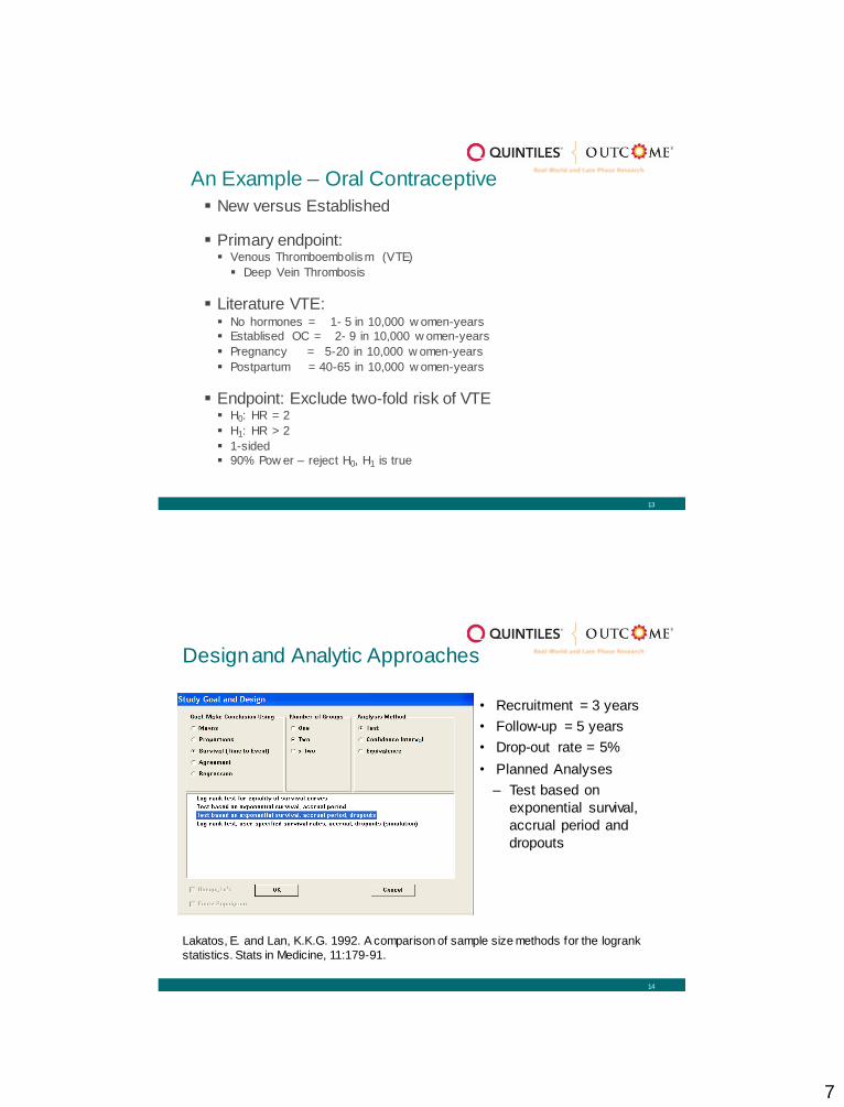
New versus Established
Primary endpoint: Venous Thromboembolism (VTE)
Deep Vein Thrombosis
Literature VTE: No hormones = 1- 5 in 10,000 w omen-years
Establised OC = 2- 9 in 10,000 w omen-years
Pregnancy = 5-20 in 10,000 w omen-years
Postpartum = 40-65 in 10,000 w omen-years
Endpoint: Exclude two-fold risk of VTE H0: HR = 2
H1: HR > 2
1-sided
90% Pow er – reject H0, H1 is true
An Example – Oral Contraceptive
14
Design and Analytic Approaches
• Recruitment = 3 years
• Follow-up = 5 years
• Drop-out rate = 5%
• Planned Analyses
– Test based on
exponential survival,
accrual period and
dropouts
Lakatos, E. and Lan, K.K.G. 1992. A comparison of sample size methods for the logrank
statistics. Stats in Medicine, 11:179-91.

8
15
Method
• 90% Power, 1-sided • z(1-α)=1.64 (5%, 1-sided)
• Z(1-β)=1.28 (90% Power)
• HR = Hazard Ratio = 2 (note: HR≠1)
• Total Events = 71
• π = 0.5 (1:1, ratio of sample in each group)
2
2
21
2
11
)]HR[ln(
34event
)]HR[ln(event
zz
16
o
TdTTd
Td
ee
dP
11
11
101
1)(E
• T0 = Accrual rate = 3 years
• T = Follow-up rate = 5 years • D = drop out rate = 5%
• λ=event rate (events per women-year)
• E(P) = expected event proportion (events per women)
• E(P1,new)=12.7 (events per 10,000W) in study
• E(P2,est) = 6.39 (events per 10,000W) in study
Method
9
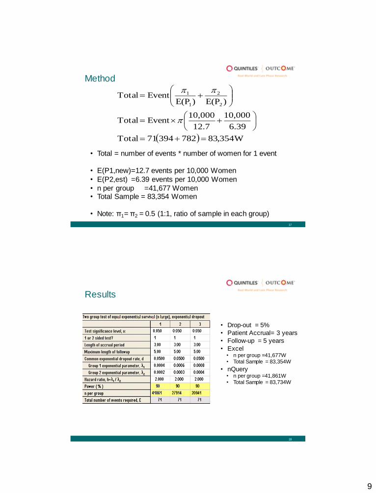
17
W354,8378239471Total
6.39
10,000
12.7
10,000EventTotal
)E(P)E(PEventTotal
2
2
1
1
• Total = number of events * number of women for 1 event
• E(P1,new)=12.7 events per 10,000 Women
• E(P2,est) =6.39 events per 10,000 Women
• n per group =41,677 Women • Total Sample = 83,354 Women
• Note: π1= π2 = 0.5 (1:1, ratio of sample in each group)
Method
18
Results
• Drop-out = 5%
• Patient Accrual= 3 years
• Follow-up = 5 years
• Excel • n per group =41,677W
• Total Sample = 83,354W
• nQuery • n per group =41,861W
• Total Sample = 83,734W
10
19
Summary for Time–to-Event
• Case Study
> VTE incidence rates per Women years
> Hazard Ratio
• Method
> Events
> Expected proportion of events
> Total number
• Results
> nQuery
20
Sample Size Estimation for a Single Cohort Dr. Pablo Mallaina
Andrew Burgess, BSc

11
21
CV Risk assessment among smokers in Primary care in Europe
Study design: > Observational, multi-centre, European, cross-sectional study (single cohort)
Objectives: > To evaluate the CVD risk among smokers at PC in Europe using standard risk assessment
tools
- Multi-factorial risk models
» Framingham Risk Score
» Systemic Coronary Risk Evaluation (SCORE)
» Progetto CUORE
> To estimate the CVD risk attributable to smoking
Sample size calculation:
> Deterministic sample size using Framingham 10-year CVD risk
Example: CV Aspire
22
• Simple case: No comparisons, binary outcome
• No power calculation – no hypothesis
• Considerations
> Desired level of precision
> Expected endpoint (percentage/rate)
> Cost and logistics of recruiting subjects
• Range of sample sizes: balance costs versus precision.
Sample Size Based on Precision of Estimate
12
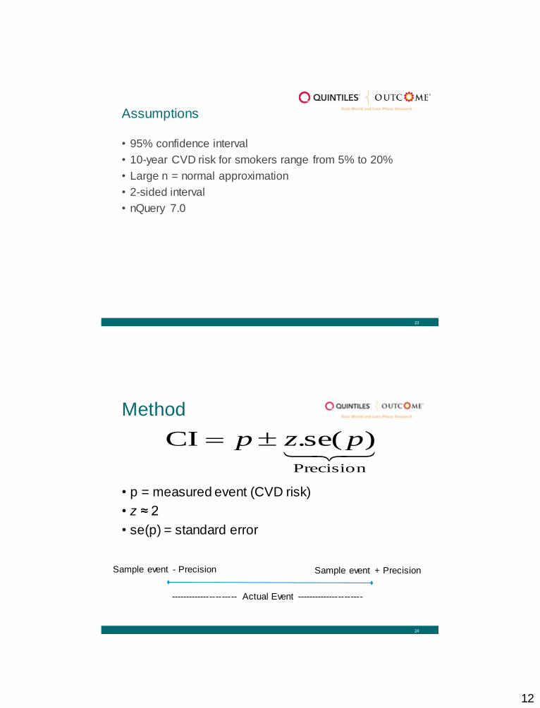
23
• 95% confidence interval
• 10-year CVD risk for smokers range from 5% to 20%
• Large n = normal approximation
• 2-sided interval
• nQuery 7.0
Assumptions
24
Method
• p = measured event (CVD risk)
• z ≈ 2
• se(p) = standard error
Precision
)se(.CI pzp
Sample event - Precision Sample event + Precision
---------------------- Actual Event ----------------------
13
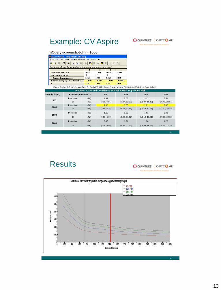
25
Example: CV Aspire
nQuery Advisor 7.0 is as follows :Janet D. Elashoff (2007) nQuery Advisor Version 7.0. Statistical Solutions, Cork, Ireland
nQuery screenshot of n = 1000
Precision Level and Confidence Interval at each Population Risk
Sample Size ↓ Expected proportion → 5% 10% 15% 20%
500 Precision (% ) 1.91 2.63 3.13 3.51
CI (% ) (3.09, 6.91) (7.37, 12.63) (11.87, 18.13) (16.49, 23.51)
1000 Precision (% ) 1.35 1.86 2.21 2.48
CI (% ) (3.65, 6.35) (8.14, 11.86) (12.79, 17.21) (17.52, 22.48)
1500 Precision (% ) 1.10 1.52 1.81 2.02
CI (% ) (3.90, 6.10) (8.48, 11.52) (13.19, 16.81) (17.89, 22.02)
2000 Precision (% ) 0.96 1.31 1.56 1.75
CI (% ) (4.04, 5.96) (8.69, 11.31) (13.44, 16.56) (18.25, 21.75)
26
Number of Patients
0 200 400 600 800 1000 1200 1400 1600 1800 2000 2200 2400 2600 2800 3000
Precisio
n
0
0.01
0.02
0.03
0.04
0.05
0.06
Confidence interval for proportion using normal approximation (n large)
5% Risk10% Risk15% Risk20% Risk
Results
14
27
CV Aspire : Summary
• Number of patients in the study = 1,439
• The CVD risk among smokers is = 21.2%
> (Framingham 10-year CVD score)
• The final precision = 2.1%
• 95% Confident that actual risk = 19.1% to 23.3%
• Objective:
>The relative increase in CVD risk attributable to
smoking = 31.9%
- The CVD risk in simulated non-smoker = 16.0%
28
Summary for
Precision
• Case Study
>CV Aspire
• Method
>Number of patients - precision
• Results
>nQuery

15
29
Sample Size Estimation to Support Generalisability of Results Eric Gemmen, MA
30
What does it mean for the
sample to be ‘representative’?
Treatment
Patterns
Health
Economic
Disease /
Epidemiology
Study Objective
Site / Phy sician Patient
Target Population Level
Possible Strata
Phy sician Specialty
Geography
Practice Size
Age, Gender
Disease & Tx Duration
16
31
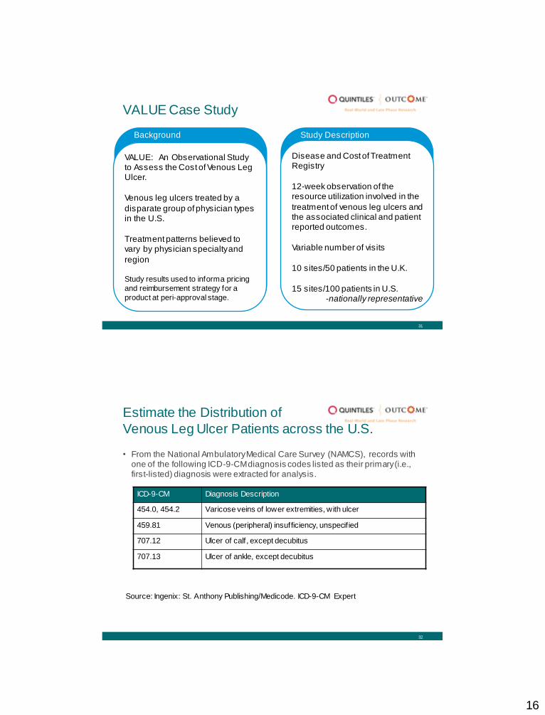
VALUE Case Study
VALUE: An Observational Study to Assess the Cost of Venous Leg Ulcer.
Venous leg ulcers treated by a
disparate group of physician types in the U.S.
Treatment patterns believed to vary by physician specialty and
region Study results used to inform a pricing
and reimbursement strategy for a
product at peri-approval stage.
Background
Disease and Cost of Treatment Registry
12-week observation of the resource utilization involved in the
treatment of venous leg ulcers and the associated clinical and patient reported outcomes.
Variable number of visits
10 sites/50 patients in the U.K.
15 sites/100 patients in U.S. -nationally representative
Study Description
32
Estimate the Distribution of
Venous Leg Ulcer Patients across the U.S.
• From the National Ambulatory Medical Care Survey (NAMCS), records with one of the following ICD-9-CM diagnosis codes listed as their primary (i.e., first-listed) diagnosis were extracted for analysis.
ICD-9-CM Diagnosis Description
454.0, 454.2 Varicose veins of lower extremities, with ulcer
459.81 Venous (peripheral) insufficiency, unspecif ied
707.12 Ulcer of calf, except decubitus
707.13 Ulcer of ankle, except decubitus
Source: Ingenix: St. Anthony Publishing/Medicode. ICD-9-CM Expert
17
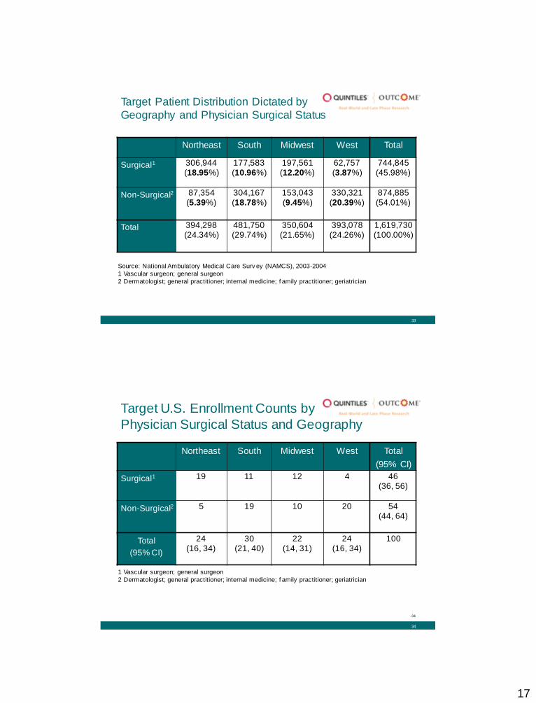
33
Target Patient Distribution Dictated by
Geography and Physician Surgical Status
Northeast South Midwest West Total
Surgical1 306,944 (18.95%)
177,583 (10.96%)
197,561 (12.20%)
62,757 (3.87%)
744,845 (45.98%)
Non-Surgical2 87,354 (5.39%)
304,167 (18.78%)
153,043 (9.45%)
330,321 (20.39%)
874,885 (54.01%)
Total 394,298 (24.34%)
481,750 (29.74%)
350,604 (21.65%)
393,078 (24.26%)
1,619,730 (100.00%)
Source: National Ambulatory Medical Care Surv ey (NAMCS), 2003-2004
1 Vascular surgeon; general surgeon
2 Dermatologist; general practitioner; internal medicine; f amily practitioner; geriatrician
34
Target U.S. Enrollment Counts by
Physician Surgical Status and Geography
Northeast South Midwest West Total
(95% CI)
Surgical1 19 11 12 4 46 (36, 56)
Non-Surgical2 5 19 10 20 54 (44, 64)
Total
(95% CI)
24 (16, 34)
30 (21, 40)
22 (14, 31)
24 (16, 34)
100
1 Vascular surgeon; general surgeon
2 Dermatologist; general practitioner; internal medicine; f amily practitioner; geriatrician
34
18
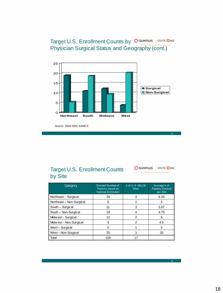
35
Target U.S. Enrollment Counts by
Physician Surgical Status and Geography (cont.)
0
5
10
15
20
25
Northeast South Midwest West
Surgical
Non-Surgical
Source: 2003-2004 NAMCS
36
Target U.S. Enrollment Counts
by Site
Category Desired Number of
Patients based on
National Estimates
# of U.S. VALUE
Sites
Av erage # of
Patients Desired
per Site
Northeast – Surgical 19 3 6.33
Northeast – Non-Surgical 5 1 5
South – Surgical 11 3 3.67
South – Non-Surgical 19 4 4.75
Midw est – Surgical 12 2 6
Midw est – Non-Surgical 9 2 4.5
West – Surgical 5 1 5
West – Non-Surgical 20 1 20
Total 100 17


