

Numerical Investigation of Turbulent Flow Through Bar racks in Closed ConduitsThrough Bar racks in Closed Conduits
Samuel Paul and Haitham GhamrySamuel Paul and Haitham Ghamry
Fi h i & O C d (DFO)Fisheries & Oceans Canada (DFO)Freshwater Institute
Winnipeg, MB

Outline
• Background• Objective• Previous Work• Problem Definition• Methodology• Methodology• Results and Discussion• Concluding Remarks• Future WorkFuture Work
2Outline
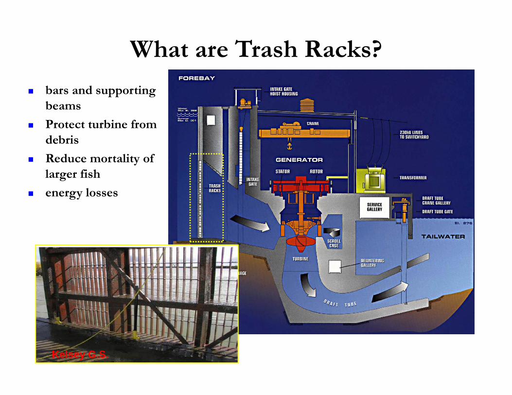
What are Trash Racks?
bars and supporting beams
Protect t rbine from Protect turbine from debris
Reduce mortality of larger fishlarger fish
energy losses
Kelsey G.S.

Trash rack in closed conduitsTrash rack in closed conduits
Trash rack in open channelTrash rack in open channel

Fish injury or mortalityFish injury or mortality
Reducing fish injury or mortality depends on:• Species, sizes, abilities and behaviourp• Spacing between bars (physical exclusion)• Shape of the barsp• Flow conditions near barracks, particularly
magnitude and patterns of flow velocity, g p yacceleration and turbulence fields
• Turbine design
zFlow z' z"2B zFlow z' z"2B
Wch
Rounded leading edge (RD)
z
Square leading edge (SQ) inclined
x
bs
ba
x'x
bs
ba
x'x(e)x
(c)

Ud
h∆h
Salient feature of this flow is yU∞
Lch
h1 h2that it produces head loss.
• These energy losses can be partly attributed to the turbulent largescale flow structures generated by the bars.g
• Both from the fish protection and head loss perspectives, it isi l di h i d d fimportant to accurately predict the magnitude and patterns ofturbulent flow characteristics, and velocity fields around and betweenthe bars.
• The ability to correctly predict complex turbulent flows isfundamental to the design of trash racks as well as other fluidengineering systems.

Objectives
• To perform numerical investigation of turbulent flowthrough arrays of rectangular bar models of variousg y gconfigurations in closed conduits using a commercialCFD code, ANSYS CFX 12.1. .
• To evaluate and validate several turbulence models inorder to assess the most suitable model for predictingorder to assess the most suitable model for predictingturbulent flow through bar racks closed conduit model
• Assess the streamlines and contours of the meanvelocity, turbulence levels, pressure field. As well asthe profiles.
7Objective

Problem Description
Wall
W
Inlet
z
Outlet
WchU∞xy 0
P = ghWall
Ps = gh
LXup Xds
8
Schematic of the flow field around bar racks and solution domainnomenclature
Problem Description
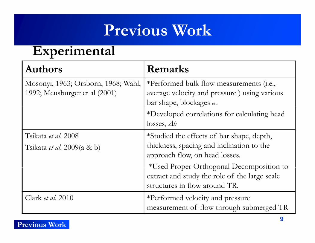
Previous WorkExperimental
Authors RemarksMosonyi, 1963; Orsborn, 1968; Wahl, 1992; Meusburger et al (2001)
*Performed bulk flow measurements (i.e., average velocity and pressure ) using various bar shape, blockages etcp g*Developed correlations for calculating head losses, h
Tsikata et al 2008 *Studied the effects of bar shape depthTsikata et al. 2008Tsikata et al. 2009(a & b)
Studied the effects of bar shape, depth, thickness, spacing and inclination to the approach flow, on head losses.*Used Proper Orthogonal Decomposition toUsed Proper Orthogonal Decomposition to extract and study the role of the large scale structures in flow around TR.
Clark et al 2010 *Performed velocity and pressure
9
Clark et al. 2010 *Performed velocity and pressure measurement of flow through submerged TR
Previous Work
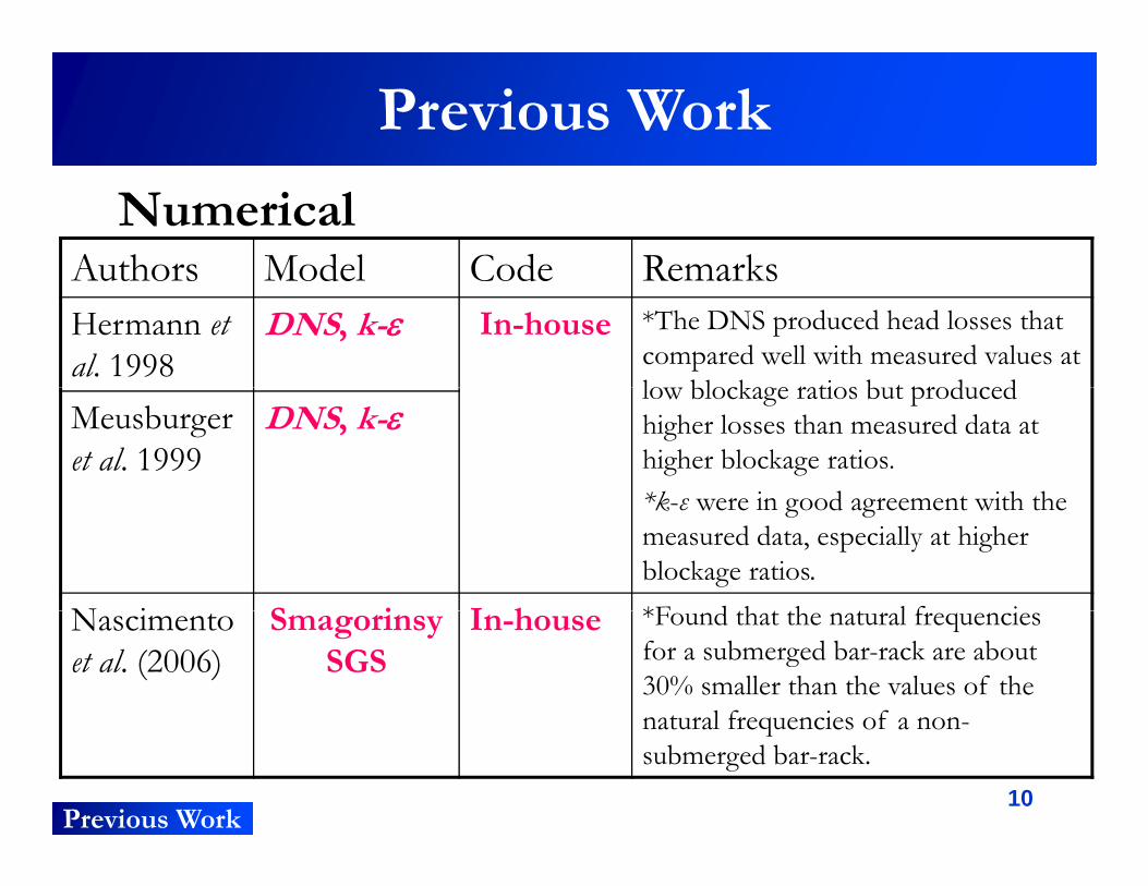
Previous Work
NumericalAuthors Model Code RemarksAuthors Model Code RemarksHermann et al. 1998
DNS, k- In-house *The DNS produced head losses that compared well with measured values at lo blockage ratios b t prod cedlow blockage ratios but produced higher losses than measured data at higher blockage ratios. *k ε were in good agreement with the
Meusburger et al. 1999
DNS, k-
*k-ε were in good agreement with the measured data, especially at higher blockage ratios.
N i S i I h *F d th t th t l f iNascimento et al. (2006)
Smagorinsy SGS
In-house *Found that the natural frequencies for a submerged bar-rack are about 30% smaller than the values of the natural frequencies of a non
10Previous Work
natural frequencies of a non-submerged bar-rack.

Present Work
Summary of geometric parameters and test conditions(University of Manitoba Experimental data for closed conduits by Clark et al.
TEST n s L b p U∞
( y p y2010, supported by Manitoba Hydro used for validation)
TEST[m]
L[m] [m]
p ∞
[m/s]
1 3 0 012 0 100 0 140 0 079 0 32 0 48 0 961 3 0.012 0.100 0.140 0.079 0.32, 0.48, 0.96,
1.12,1.37, 1.64
2 7 0.012 0.100 0.053 0.185 0.49, 0.98, 1.39
3 14 0.012 0 100 0.021 0.369 0.26, 0.78, 1.42
11Problem Description
3 14 0.012 0.100 0.021 0.369 0.26, 0.78, 1.42
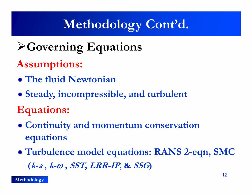
Methodology Cont’d.
Governing EquationsA iAssumptions:
The fluid Newtonian
Steady, incompressible, and turbulent
Equations:Equations:Continuity and momentum conservation
iequations
Turbulence model equations: RANS 2-eqn, SMC(k-ε , k- , SST, LRR-IP, & SSG)
12Methodology
Methodology
Numerical Solution
Commercial CFD Code, ANSYS CFX v12.0:• Element based FVM• Element based FVM• Geometrical representation and integration points are based on FEM
• The coupled discretized mass and momentum equations with the turbulence model equations were solved iteratively using additive
i l i id l icorrection multi-grid acceleration. • Solutions were considered converged when the normalized maximum
residual of all the discretized equations was less than 1×10⁻⁴.residual of all the discretized equations was less than 1 10 .
13Methodology
Methodology Cont’d.
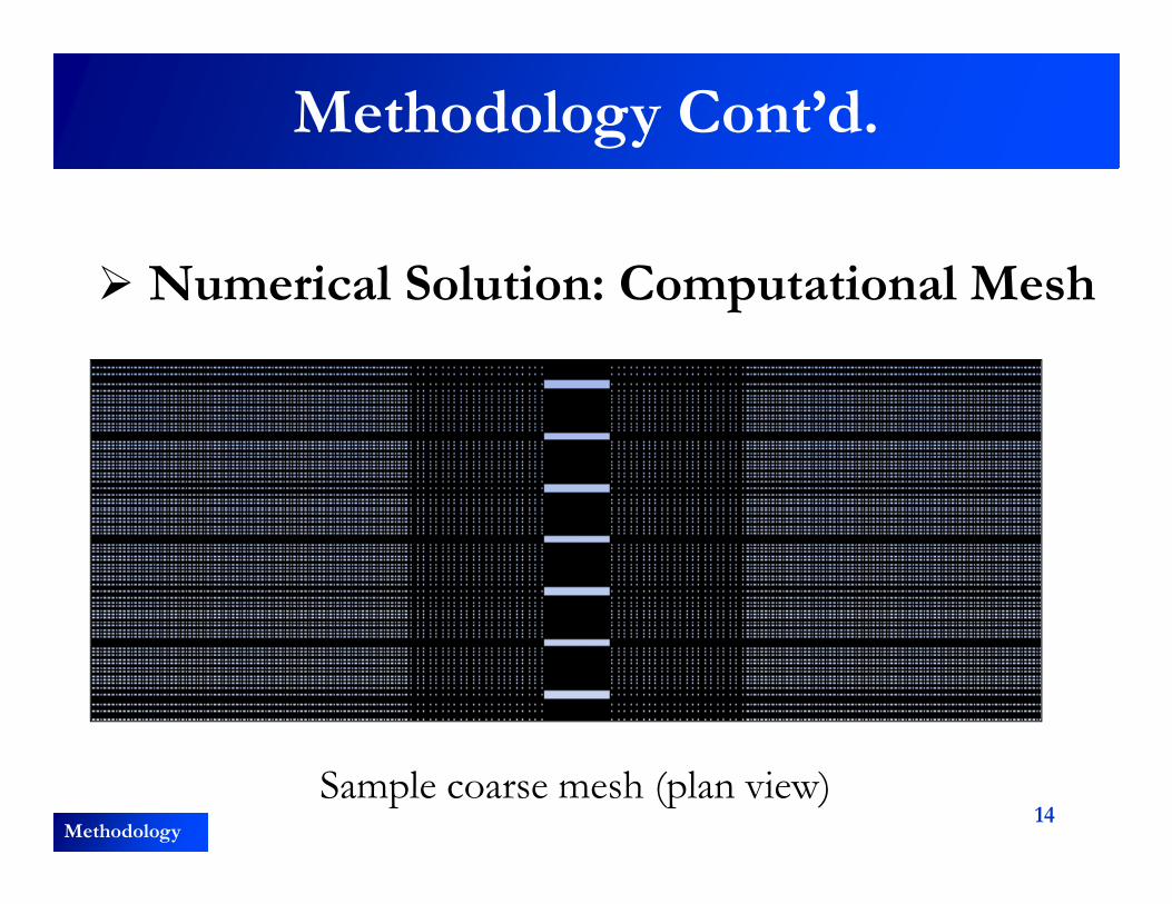
Numerical Solution: Computational Mesh Numerical Solution: Computational Mesh
14Methodology
Sample coarse mesh (plan view)

Methodology Cont’d.
Numerical Solution: Boundary conditions
I l tI l t O tl tO tl tInletInlet OutletOutlet• U = U∞, I = 0.05 Ps = gh
WallsWalls• N li• No-slip
• Low Reynolds number near-wall treatmentLow Reynolds number near wall treatmentfor all models
15Methodology
Results & Discussion
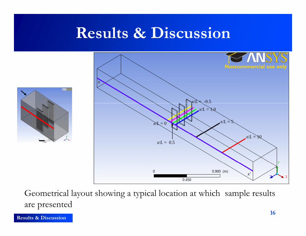
x/L = -0.5
x
x/L = 5x/L = 0
x/L = 1.0
x/L = 10x/L = 0.5
Geometrical layout showing a typical location at which sample results
x'
16
Geometrical layout showing a typical location at which sample results are presented
Results & Discussion

Results & Discussion Cont’d.
0 14
0.16
7bars, U = 0.49 m/s
Present Num. Study: k-
k-
0.16
E i t l d t
3bars, U = 0.48 m/s
-1.5 -1.0 -0.5 0.0 0.5 1.0 1.50.12
0.14 k SST LRR O-Based
Expt.[Clark et al. 2010] (a)
-1.5 -1.0 -0.5 0.0 0.5 1.0 1.50.12
0.14 Experimental data Present Num. Study: k- k- SST (d)
0 16
0.20
0.247bars, U
= 0.98 m/s
h[m]
016
0.20
0.24
h[m]
3bars, U = 0.96 m/s
-1.5 -1.0 -0.5 0.0 0.5 1.0 1.50.12
0.16
(b)
0 28
0.327bars, U = 1.39 m/s
-1.5 -1.0 -0.5 0.0 0.5 1.0 1.50.12
0.16
(e)
0.283bars, U
= 1.37 m/s
0.16
0.20
0.24
0.28 7ba s, U
.39 /s
( )
0.16
0.20
0.24
(f)
17Results & Discussion
Comparison between profiles of predicted pressure head with measured values for selected approach velocity: (a, b, c) 7 bars and (e, f, g) 3 bars.
x[m]-1.5 -1.0 -0.5 0.0 0.5 1.0 1.5
0.12 (c)
x[m]-1.5 -1.0 -0.5 0.0 0.5 1.0 1.5
0.12(f)

Results & Discussion Cont’d.
N i l S d E
TableTable 11:: SummarySummary ofof headhead lossloss coefficientcoefficient forfor TestTest 22
Model L(m) np
U∞(m/s) Numerical Study Expt.∆h ∆h* ∆h*
k-ε0.10 7 0.185 0.49 0.0042 0.343 0.334
0.10 7 0.185 0.98 0.0170 0.343 0.334
0.10 7 0.185 1.39 0.0340 0.343 0.334
k-ω0.10 7 0.185 0.49 0.0044 0.360 0.3340.10 7 0.185 0.98 0.0180 0.360 0.3340.10 7 0.185 1.39 0.0350 0.360 0.334
SST0.10 7 0.185 0.49 0.0043 0.351 0.3340.10 7 0.185 0.98 0.0170 0.351 0.3340.10 7 0.185 1.39 0.0350 0.351 0.3340. 0 7 0. 85 .39 0.0350 0.35 0.334
LRR-IP0.10 7 0.185 0.49 0.0040 0.347 0.3340.10 7 0.185 0.98 0.0170 0.347 0.3340.10 7 0.185 1.39 0.034 0.347 0.334
18Results & Discussion
SSG0.10 7 0.185 0.49 0.0040 0.351 0.3340.10 7 0.185 0.98 0.0172 0.351 0.3340.10 7 0.185 1.39 0.0346 0.351 0.334
Results & Discussion Cont’d.
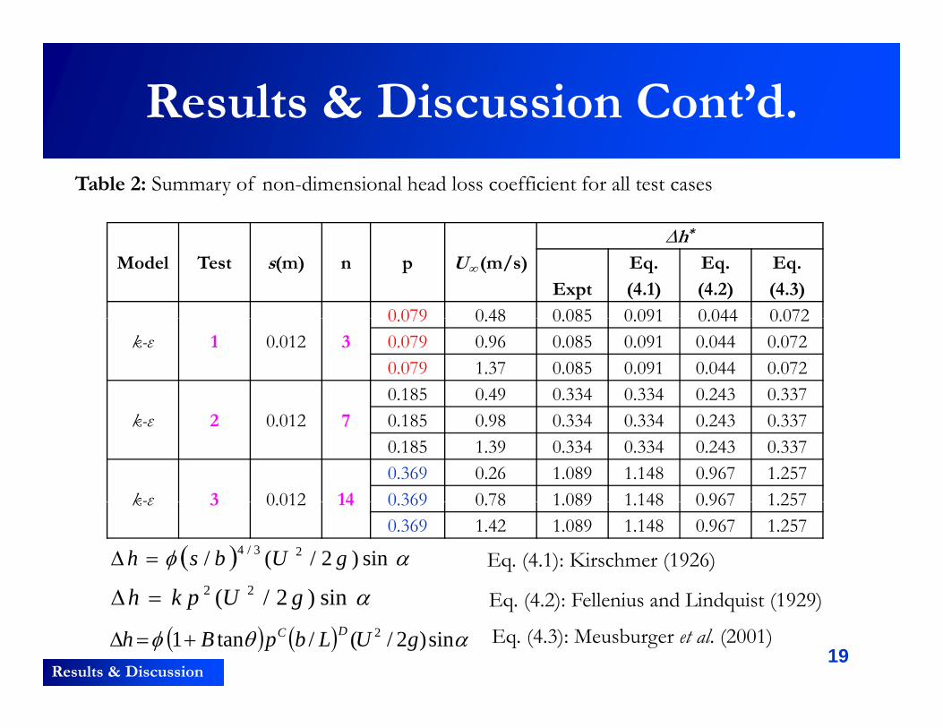
Table 2: Summary of non-dimensional head loss coefficient for all test cases
Model Test s(m) n p U∞ (m/s)
∆h*
Expt
Eq.
(4.1)
Eq.
(4.2)
Eq.
(4.3)
0 079 0 48 0 085 0 091 0 044 0 072k-ε 1 0.012 3
0.079 0.48 0.085 0.091 0.044 0.0720.079 0.96 0.085 0.091 0.044 0.0720.079 1.37 0.085 0.091 0.044 0.0720.185 0.49 0.334 0.334 0.243 0.337
k-ε 2 0.012 7 0.185 0.98 0.334 0.334 0.243 0.3370.185 1.39 0.334 0.334 0.243 0.337
k-ε 3 0 012 14
0.369 0.26 1.089 1.148 0.967 1.2570 369 0 78 1 089 1 148 0 967 1 257k-ε 3 0.012 14 0.369 0.78 1.089 1.148 0.967 1.2570.369 1.42 1.089 1.148 0.967 1.257
sin)2/(/ 23/4 gUbsh
i)2/( 22 Ukh
Eq. (4.1): Kirschmer (1926)
E (4 2) F ll i d Li d i (1929)
19Results & Discussion
sin)2/( 22 gUpkh
sin)2/(/tan1 2 gULbpBh DC
Eq. (4.2): Fellenius and Lindquist (1929)
Eq. (4.3): Meusburger et al. (2001)

Results & Discussion Cont’d.
(a) (b)
20
Contours of: (a) mean streamwise velocity and (b) static pressure field
Results & Discussion

Results & Discussion Cont’d.
(a) (d)
(b) (e)
(c) (f)
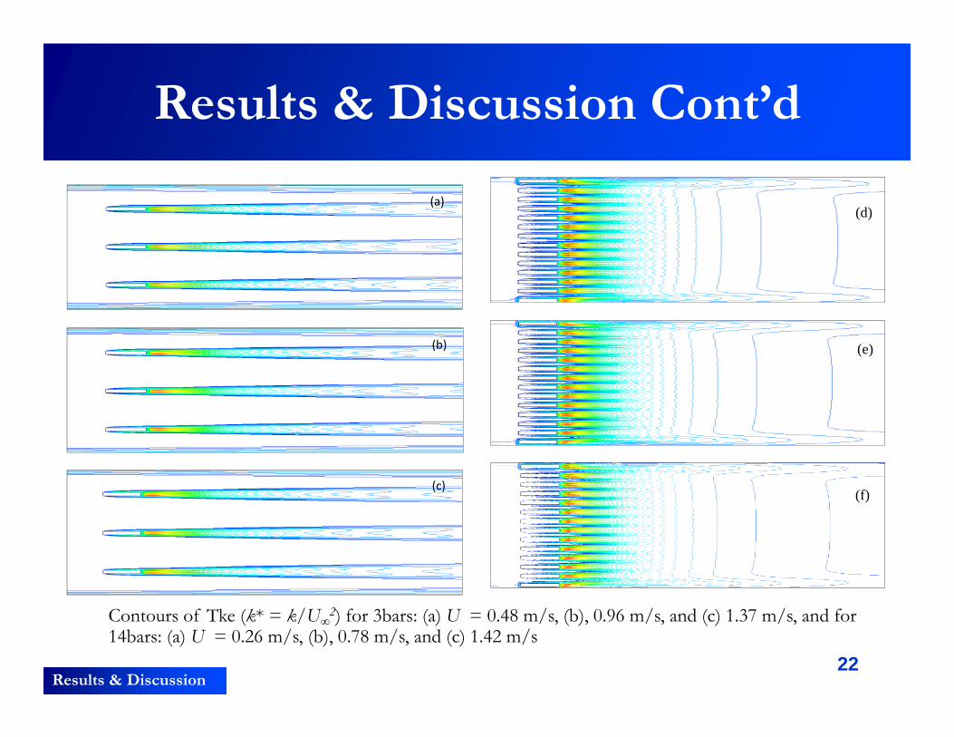
21Results & Discussion
Contours of mean velocity (U* = U/U∞) for 3bars: (a) U = 0.48 m/s, (b), 0.96 m/s, and (c) 1.37 m/s, and for 14bars: (a) U = 0.26 m/s, (b), 0.78 m/s, and (c) 1.42 m/s
Results & Discussion Cont’d
(d)(a)
(e)(b)
(f)(c)
22Results & Discussion
Contours of Tke (k* = k/U∞2) for 3bars: (a) U = 0.48 m/s, (b), 0.96 m/s, and (c) 1.37 m/s, and for
14bars: (a) U = 0.26 m/s, (b), 0.78 m/s, and (c) 1.42 m/s

Results & Discussion Cont’d
05
1.0(a)U/U
(b) (c)
0.0
0.5 U = 0.48 m/s U = 0.96 m/s U = 1.37 m/s
U = 0.49 m/s U = 0.98 m/s U = 1.39 m/s
U = 0.26 m/s U = 0.78 m/s U = 1.42 m/s
0 5 10 150 5 10 15/
0 5 10 15 20
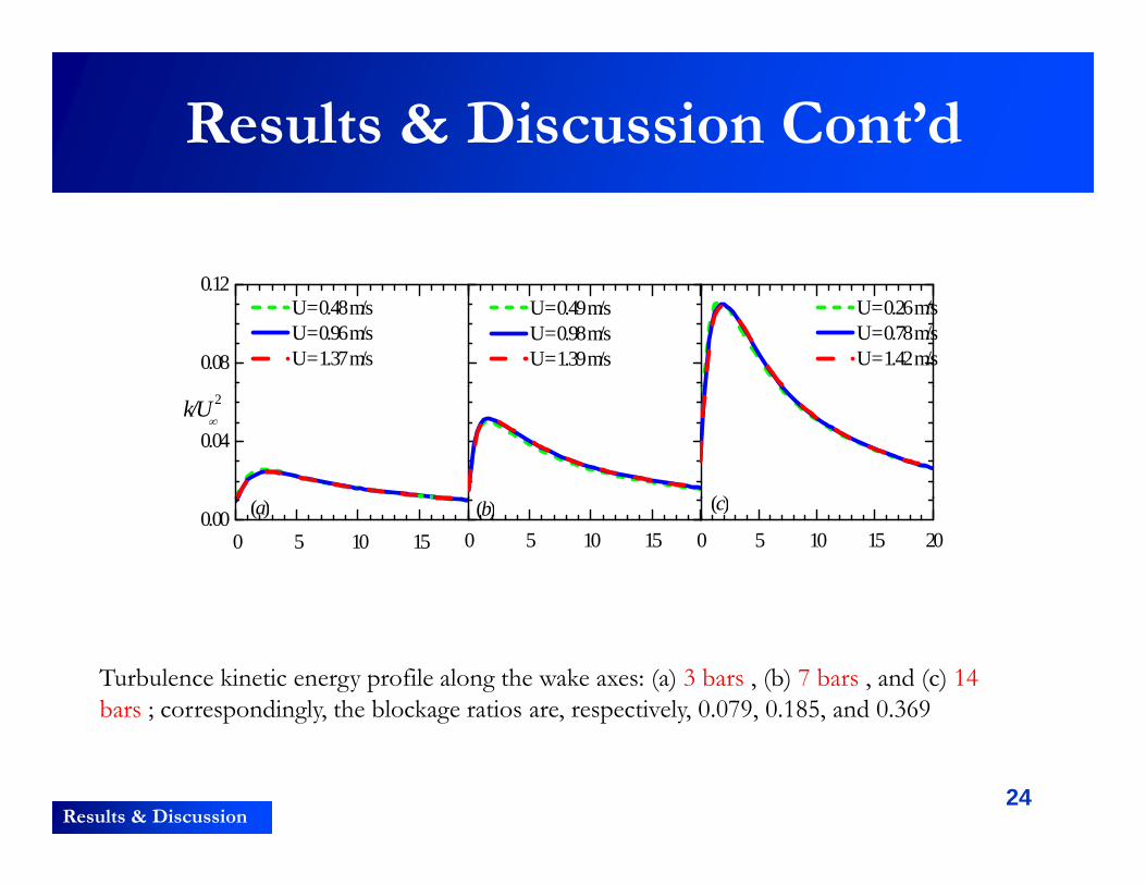
Mean velocity profile along the wake axes; (a) 3 bars , (b) 7 bars , and (c) 14 bars ; correspondingly, the blockage ratios are, respectively, 0.079, 0.185, and 0.369
23Results & Discussion
Results & Discussion Cont’d
0.08
0.12 U = 0.48 m/s U = 0.96 m/s U = 1.37 m/s
U = 0.49 m/s U = 0.98 m/s U = 1.39 m/s
U = 0.26 m/s U = 0.78 m/s U = 1.42 m/s
0.04k/U
2
( )
0 5 10 150 5 10 150.00 (a) (b)
0 5 10 15 20
(c)
Turbulence kinetic energy profile along the wake axes: (a) 3 bars , (b) 7 bars , and (c) 14 bars ; correspondingly, the blockage ratios are, respectively, 0.079, 0.185, and 0.369
24Results & Discussion
p g y g p y
Results & Discussion Cont’d2.5
10.05.01.0x/L = 0
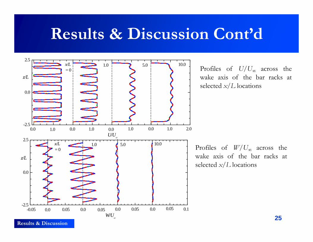
/Profiles of U/U∞ across the
k i f h b k
0.0
z/L wake axis of the bar racks atselected x/L locations
-2.51.01.01.01.0 2.00.00.00.0
U/U0.0
U/U2.5
z/L
10.05.01.0x/L = 0 Profiles of W/U∞ across the
wake axis of the bar racks atselected x/L locations
0.0se ected x/ ocat o s
25Results & Discussion
-2.50.050.00.00.00.0 0.10.050.050.05
W/U
-0.05

Concluding Remarks The ANSYS-CFX reproduces the flow characteristics reasonably
well
k- models give better results than the other models
Present results were in good agreement with prior results
k- model predicted the mean velocity, turbulence kinetic energy, and pressure coefficient reasonably well. It was found that the head loss increases with blockage ratio as well as the independence of dimensionless pressure head (∆h*) on the Reynolds number.y
The recovery of mean velocity to its upstream value (U/U∞= 1) is most rapid at higher blockage ratio.
the level of turbulence increases with increasing blockage ratio26
Future works

Future Works
• Will provide further insight into the effects of bar leading andtrailing edges bar shape bar depth bar thickness bar spacing andtrailing edges, bar shape, bar depth, bar thickness, bar spacing andbar inclination to the approach flow, on head losses in model barracks using Flow 3-D software for improved bar rack design andfish survival at hydroelectric turbines.
• Influence of the following flow parameters on fish survival:• Influence of the following flow parameters on fish survival:– Turbulence and turbulence intensity (area upstream of bar racks)– Shear in flow (area upstream of bar racks)Shear in flow (area upstream of bar racks)– Acceleration (area upstream of bar racks)– Areas of maximum flow speed (area upstream of bar racks)will be fully examined.
27Future works

Acknowledgement
Profound gratitude to:
DFO-CHIF
UNIVERSITY OF MANITOBA
MANITOBA HYDROMANITOBA HYDRO
HYDRONET NSERC
for their support
28Acknowledgement

Question
29Question


