

Scheduling and Fairness in Multi-hop WirelessNetworks
Ananth Rao
Electrical Engineering and Computer SciencesUniversity of California at Berkeley
Technical Report No. UCB/EECS-2007-150
http://www.eecs.berkeley.edu/Pubs/TechRpts/2007/EECS-2007-150.html
December 13, 2007

Copyright © 2007, by the author(s).All rights reserved.
Permission to make digital or hard copies of all or part of this work forpersonal or classroom use is granted without fee provided that copies arenot made or distributed for profit or commercial advantage and that copiesbear this notice and the full citation on the first page. To copy otherwise, torepublish, to post on servers or to redistribute to lists, requires prior specificpermission.
Scheduling and Fairness in Multi-hop Wireless Networks
by
Ananthapadmanabha Rajagopala-Rao
B.Tech. (Indian Institute of Technology, Madras, India) 2001M.S. (University of California, Berkeley) 2004
A dissertation submitted in partial satisfactionof the requirements for the degree of
Doctor of Philosophy
in
Computer Science
in the
GRADUATE DIVISION
of the
UNIVERSITY OF CALIFORNIA, BERKELEY
Committee in charge:
Professor Ion Stoica, ChairProfessor Scott ShenkerProfessor John Chuang
Fall 2007

The dissertation of Ananthapadmanabha Rajagopala-Rao is approved.
Chair Date
Date
Date
University of California, Berkeley
Fall 2007

Scheduling and Fairness in Multi-hop Wireless Networks
Copyright c© 2007
by
Ananthapadmanabha Rajagopala-Rao
Abstract
Scheduling and Fairness in Multi-hop Wireless Networks
by
Ananthapadmanabha Rajagopala-Rao
Doctor of Philosophy in Computer Science
University of California, Berkeley
Professor Ion Stoica, Chair
Multi-hop wireless networks have been a subject of research for many years now. But
recently, availability of inexpensive hardware has spurred interest in a new class of
applications called mesh networks where multi-hop wireless routing is used to avoid
the cost of deploying a wired backbone. However, both simulations and deployments
based on the current generation of hardware (based mostly on the 802.11 standard)
show very poor fairness between competing flows. In fact, the imbalance in through-
put can be so severe that some nodes are completely shut out from sending any data
at all. Some of this unfairness can be attributed to the lack of flexibility in the
802.11 Medium Access Control (MAC) layer to provide control over resource alloca-
tion. Recent work also suggests that Carrier-Sense Multiple Access (CSMA) based
MAC protocols suffer from a more fundamental limitation due to problems caused by
hidden terminals and asymmetric links.
In this work, we address this problem by making the following three contribu-
tions. Firstly, we build an Overlay MAC Layer (OML) that implements a time-slot
based scheduler that works on top of inexpensive 802.11 based hardware without
1
any changes to the standard. The overlay approach also provides a lot of flexibil-
ity and can easily be adapted to specific applications and networks through simple
software modifications. Secondly, we have developed a distributed algorithm that
can efficiently detect interference by using passive measurements. While we use the
inferred interference pattern to improve scheduling under OML, our algorithm can
also be used in a number of other applications such as channel assignment, resource
allocation and admission control. Thirdly, we have designed a transport layer algo-
rithm called End-to-end Fairness using Local Weights (EFLoW) for providing global
Max-Min Fairness. EFLoW uses an iterative additive-increase multiplicative-decrease
(AIMD) based approach using only state from within a given node’s contention re-
gion in each iteration. It can automatically adapt to changes in traffic demands and
network conditions.
We have evaluated our system by conducting experiments in both ns-2 and a
30-node testbed built using commodity hardware. We show that our algorithms
can improve fairness by over 90% with only a small cost (typically less than
10%) in efficiency for a wide variety of traffic patterns and network conditions.
Professor Ion StoicaDissertation Committee Chair
2

Contents
Contents i
List of Figures v
List of Tables viii
Acknowledgements ix
1 Introduction 1
1.1 Fairness in Wireless Networks . . . . . . . . . . . . . . . . . . . . . . 2
1.2 Fairness at the MAC Layer . . . . . . . . . . . . . . . . . . . . . . . . 3
1.3 Detecting Interference between Links . . . . . . . . . . . . . . . . . . 6
1.4 Fairness at the Transport Layer . . . . . . . . . . . . . . . . . . . . . 7
1.5 Organization . . . . . . . . . . . . . . . . . . . . . . . . . . . . . . . 9
2 Previous Work 10
2.1 MAC Layer . . . . . . . . . . . . . . . . . . . . . . . . . . . . . . . . 10
2.2 Detecting Interference . . . . . . . . . . . . . . . . . . . . . . . . . . 12
2.3 Transport and Higher Layers . . . . . . . . . . . . . . . . . . . . . . . 15
2.4 Other Related Work . . . . . . . . . . . . . . . . . . . . . . . . . . . 17
3 Overlay MAC Layer (OML) 20
3.1 Motivation . . . . . . . . . . . . . . . . . . . . . . . . . . . . . . . . . 20
3.1.1 Limitations of 802.11 MAC Layer . . . . . . . . . . . . . . . . 21
3.1.1.1 Effect of Asymmetric Interaction . . . . . . . . . . . 21
3.1.1.2 Sub-optimal Default Allocation . . . . . . . . . . . . 24
i

3.1.2 Need for a MAC Layer Solution . . . . . . . . . . . . . . . . . 26
3.1.3 Advantages of an Overlay Solution . . . . . . . . . . . . . . . 27
3.2 Design . . . . . . . . . . . . . . . . . . . . . . . . . . . . . . . . . . . 28
3.2.1 Assumptions . . . . . . . . . . . . . . . . . . . . . . . . . . . . 29
3.2.2 Solution . . . . . . . . . . . . . . . . . . . . . . . . . . . . . . 30
3.2.2.1 Slot size . . . . . . . . . . . . . . . . . . . . . . . . . 31
3.2.2.2 Clock synchronization . . . . . . . . . . . . . . . . . 32
3.2.2.3 Weighted Slot Allocation (WSA) . . . . . . . . . . . 33
3.2.2.4 Putting it all together . . . . . . . . . . . . . . . . . 38
3.3 Implementation . . . . . . . . . . . . . . . . . . . . . . . . . . . . . . 39
3.3.1 Overview of Click . . . . . . . . . . . . . . . . . . . . . . . . . 40
3.3.2 OML Elements in Click . . . . . . . . . . . . . . . . . . . . . 40
3.4 Results . . . . . . . . . . . . . . . . . . . . . . . . . . . . . . . . . . . 42
3.4.1 Heterogeneous data rates . . . . . . . . . . . . . . . . . . . . . 43
3.4.2 Chain topology . . . . . . . . . . . . . . . . . . . . . . . . . . 44
3.4.3 Multi-hop routing . . . . . . . . . . . . . . . . . . . . . . . . . 46
3.4.4 Weighted allocation . . . . . . . . . . . . . . . . . . . . . . . . 48
3.4.5 Short Flows . . . . . . . . . . . . . . . . . . . . . . . . . . . . 48
4 Detecting Interference using Passive Measurements 50
4.1 Our Approach . . . . . . . . . . . . . . . . . . . . . . . . . . . . . . . 50
4.2 Algorithm . . . . . . . . . . . . . . . . . . . . . . . . . . . . . . . . . 53
4.2.1 Definitions and Assumptions . . . . . . . . . . . . . . . . . . . 53
4.2.2 Centralized Algorithm . . . . . . . . . . . . . . . . . . . . . . 54
4.2.3 Distributed Algorithm . . . . . . . . . . . . . . . . . . . . . . 60
4.2.3.1 Scoped flooding of link information . . . . . . . . . . 61
4.2.3.2 Removing Stale Inferences . . . . . . . . . . . . . . . 63
4.3 Evaluation Methodology . . . . . . . . . . . . . . . . . . . . . . . . . 67
4.3.1 Simulation . . . . . . . . . . . . . . . . . . . . . . . . . . . . . 67
4.3.1.1 Interference pattern in simulation . . . . . . . . . . . 67
4.3.2 Implementation . . . . . . . . . . . . . . . . . . . . . . . . . . 69
4.4 Results . . . . . . . . . . . . . . . . . . . . . . . . . . . . . . . . . . . 70
ii

4.4.1 Evaluation Metrics . . . . . . . . . . . . . . . . . . . . . . . . 70
4.4.2 Simulation . . . . . . . . . . . . . . . . . . . . . . . . . . . . . 71
4.4.2.1 Accuracy of Interference Inference . . . . . . . . . . 71
4.4.2.2 Effect of Node Density . . . . . . . . . . . . . . . . . 72
4.4.2.3 Time to Detect Interference . . . . . . . . . . . . . . 73
4.4.3 Test-bed . . . . . . . . . . . . . . . . . . . . . . . . . . . . . . 73
4.4.3.1 Performance of 1-hop and 2-hop heuristics . . . . . . 74
4.4.3.2 Performance of Passive Detection . . . . . . . . . . . 75
5 End-to-end Fairness using Local Weights 77
5.1 Max-Min fairness . . . . . . . . . . . . . . . . . . . . . . . . . . . . . 77
5.1.1 Max-Min Fairness . . . . . . . . . . . . . . . . . . . . . . . . . 78
5.2 Achieving End-to-end Fairness . . . . . . . . . . . . . . . . . . . . . . 80
5.2.1 System Model . . . . . . . . . . . . . . . . . . . . . . . . . . . 80
5.2.1.1 Stage 1: Single Contention Region . . . . . . . . . . 80
5.2.1.2 Stage 2: Mutli-hop Network . . . . . . . . . . . . . . 81
5.2.2 EFLoW . . . . . . . . . . . . . . . . . . . . . . . . . . . . . . 83
5.3 Results . . . . . . . . . . . . . . . . . . . . . . . . . . . . . . . . . . . 88
5.3.1 Simulations . . . . . . . . . . . . . . . . . . . . . . . . . . . . 89
5.3.1.1 TDMA MAC Protocol . . . . . . . . . . . . . . . . . 89
5.3.1.2 Ideal Allocation . . . . . . . . . . . . . . . . . . . . . 90
5.3.1.3 Convergence of EFLoW . . . . . . . . . . . . . . . . 90
5.3.1.4 Effect of the number of flows . . . . . . . . . . . . . 94
5.3.1.5 Random flows vs. Star traffic pattern . . . . . . . . . 97
5.3.1.6 Effect of accuracy of interference information . . . . 98
5.3.1.7 TCP flows . . . . . . . . . . . . . . . . . . . . . . . . 102
5.3.1.8 Scaling Network Size . . . . . . . . . . . . . . . . . . 104
5.3.2 Test-bed . . . . . . . . . . . . . . . . . . . . . . . . . . . . . . 104
5.3.2.1 Two simultaneous flows . . . . . . . . . . . . . . . . 105
5.3.2.2 Three simultaneous flows . . . . . . . . . . . . . . . 107
5.3.2.3 Short flows . . . . . . . . . . . . . . . . . . . . . . . 108
iii

6 Conclusions 110
6.1 Open Issues and Future Work . . . . . . . . . . . . . . . . . . . . . . 112
Bibliography 115
iv
List of Figures
2.1 In the presence of RF-opaque obstacles, the 2-hop interference modelcan overestimate interference e.g., between nodes A and C. . . . . . . 13
2.2 If nodes are equipped with directional antenna, the interference-rangedoes not correlate very well with network distance. Node C is withing2 hops of node A, but is outside its interference range. . . . . . . . . 14
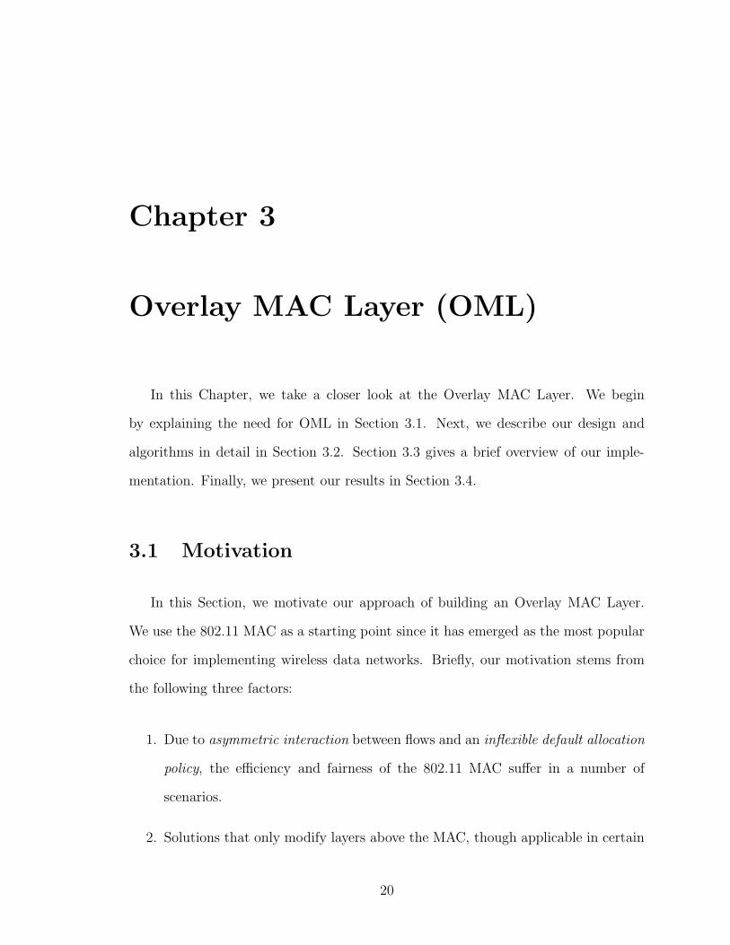
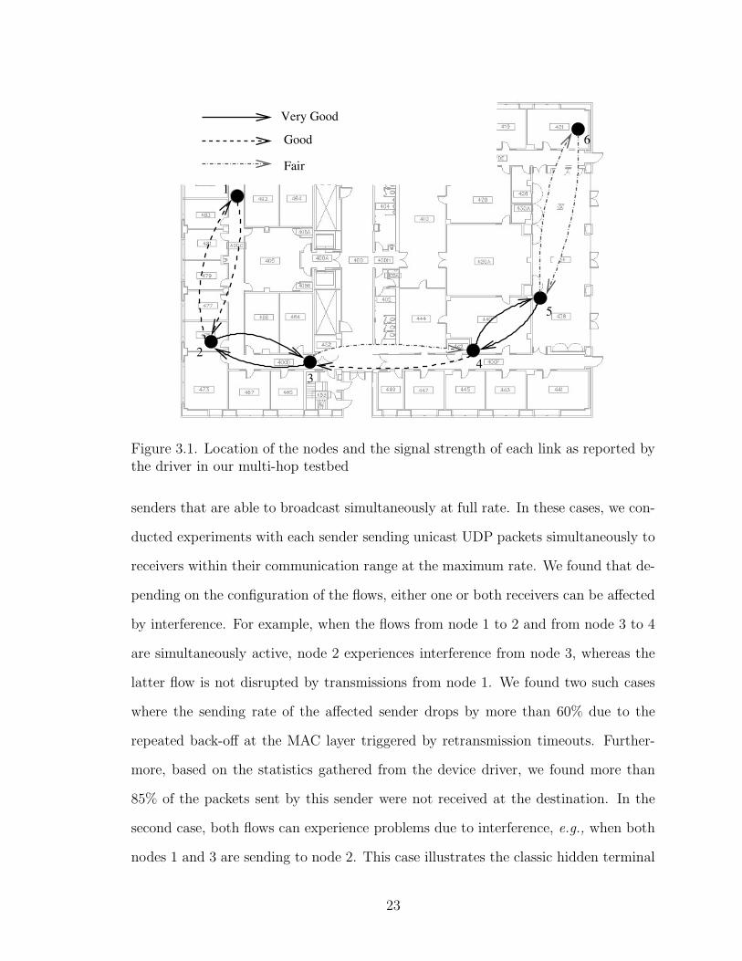
3.1 Location of the nodes and the signal strength of each link as reportedby the driver in our multi-hop testbed . . . . . . . . . . . . . . . . . 23
3.2 802.11 throughput in the presence of heterogeneous data rate senders 24
3.3 Example of interaction of multiple flows in a multi-hop network . . . 26
3.4 Click configuration for OML . . . . . . . . . . . . . . . . . . . . . . . 42
3.5 802.11 throughput in the presence of heterogeneous data rate sendersusing OML . . . . . . . . . . . . . . . . . . . . . . . . . . . . . . . . 44
3.6 CDF of throughput of 1-hop flows in the network . . . . . . . . . . . 46
4.1 The interference graph for five links in a simple network topology . . 55
4.2 An example input for our algorithm. We only show which links areactive in each time-slot. The throughput in each of these slots is alsoavailable in shi. . . . . . . . . . . . . . . . . . . . . . . . . . . . . . . 56
4.3 The graphs constructed by GetInterferingLinks(D) for the network inFigure 4.1 using the shi in Figure 4.2. We initially start with graph(a), which yields (b) after the clean-up phase. We then detect links Cand E as interfering links over two iterations; the corresponding graphsare shown in (c) and (d). . . . . . . . . . . . . . . . . . . . . . . . . 58
4.4 The pseudocode for the centralized algorithm to get the list of linksthat interfere with a given link . . . . . . . . . . . . . . . . . . . . . . 66
4.5 The gain pattern of our simulated directional antenna . . . . . . . . . 69
v

4.6 The effect of node density on the accuracy for various methods ofguessing interference . . . . . . . . . . . . . . . . . . . . . . . . . . . 73
4.7 The CDF of the time taken to detect interference . . . . . . . . . . . 74
4.8 The CDF of the time taken to detect interference in our testbed . . . 76
5.1 Example for Max-Min Fair allocation . . . . . . . . . . . . . . . . . . 79
5.2 Scheduling within a single contention neighborhood . . . . . . . . . . 82
5.3 Contention contexts in a multi-hop network . . . . . . . . . . . . . . 83
5.4 Pseudocode for the function executed by every node at the end of Wtime slots . . . . . . . . . . . . . . . . . . . . . . . . . . . . . . . . . 87
5.5 Pseudocode for the Oracle to approximate the ideal allocation . . . . 91
5.6 Effect of the additive increase parameter α on fairness. . . . . . . . . 93
5.7 Effect of the multiplicative decrease parameter β on fairness. . . . . . 93
5.8 Effect of the duration of the flows on fairness with and without EFLoW 94
5.9 Effect of the number of simultaneous flows on fairness with and withoutEFLoW when using the TDMA MAC (star traffic) . . . . . . . . . . 95
5.10 Effect of the number of simultaneous flows on fairness with and withoutEFLoW when using OML (star traffic) . . . . . . . . . . . . . . . . . 96
5.11 Effect of the number of simultaneous flows on utilization with andwithout EFLoW when using the TDMA MAC (star traffic) . . . . . . 96
5.12 Effect of the number of simultaneous flows on utilization with andwithout EFLoW when using OML (star traffic) . . . . . . . . . . . . 97
5.13 Effect of the number of simultaneous flows on fairness with and withoutEFLoW when using the TDMA MAC for the random traffic pattern . 98
5.14 Effect of the number of simultaneous flows on utilization with andwithout EFLoW when using the TDMA MAC for the random trafficpattern . . . . . . . . . . . . . . . . . . . . . . . . . . . . . . . . . . . 99
5.15 CDF of the ratio of allocation to the ideal under 802.11 and EFLoW(with TDMA MAC) for the star and random traffic patterns . . . . . 99
5.16 The effect of the interference information on fairness when usingEFLoW(Hop-based interference) . . . . . . . . . . . . . . . . . . . . . 100
5.17 The effect of the interference information on fairness when usingEFLoW(Directional antenna) . . . . . . . . . . . . . . . . . . . . . . 101
5.18 The effect of the interference information on efficiency when usingEFLoW(Hop-based interference) . . . . . . . . . . . . . . . . . . . . . 101
vi

5.19 The effect of the interference information on efficiency when usingEFLoW(Directional antenna) . . . . . . . . . . . . . . . . . . . . . . 102
5.20 Comparison of performance of TCP and UDP flows . . . . . . . . . . 103
5.21 Effect of the network size on the performance of 802.11 and EFLoW(with OML) . . . . . . . . . . . . . . . . . . . . . . . . . . . . . . . . 104
5.22 The CDF of the fairness index of two simultaneous TCP flows in thetest-bed . . . . . . . . . . . . . . . . . . . . . . . . . . . . . . . . . . 106
5.23 The CDF of the fairness index of three simultaneous TCP flows in thetest-bed . . . . . . . . . . . . . . . . . . . . . . . . . . . . . . . . . . 107
5.24 The CDF of the throughput of short flows in our test-bed . . . . . . . 108
vii

List of Tables
3.1 Average system throughput (Mbps) and fairness for two simultaneousflows . . . . . . . . . . . . . . . . . . . . . . . . . . . . . . . . . . . . 46
3.2 Interaction of flows in an ad-hoc topology . . . . . . . . . . . . . . . 47
3.3 Throughput received by senders with different weights . . . . . . . . . 48
3.4 Transfer time of a short flow in the presence of a long flow . . . . . . 48
4.1 Accuracy of interference inference for various propagation models . . 72
4.2 Performance of the 1-hop and 2-hop heuristics in our testbed . . . . . 75
5.1 Efficiency of various schemes for 2 simultaneous flows in the test-bed. 105
viii

Acknowledgements
Firstly, I would like to thank my advisor, Prof. Ion Stoica for his support through
good times and bad over the last six years. Besides providing valuable intellectual
guidance, he has been the most understanding and caring person I have ever had a
chance to work with. He perfectly carried out the balancing act of being very closely
involved with my work, yet giving me complete control and freedom over what I did.
Working with Prof. Scott Shenker is an experience I will cherish for a long time
to come. I am convinced he is both the fastest and the best person at what he does;
think about, distill and communicate great research. It was such a delight watching
him turn the most nebulous concept into a concrete, publication-worthy idea at the
blink of an eye.
In addition, I would like to thank Prof. John Chuang for finding the time admist
his busy schedule to read yet another computer science dissertation. He also served on
my qualifying exam committee and gave very useful feedback during our discussions.
Based on his extensive knowledge of computer science and networking, at times it
was hard for me to believe he was actually the external member!
My research would not have been possible without the generosity of Prof. Robert
Morris, who allowed us to use the test-bed set up by his group at MIT. I also received
technical assistance from several of his students including John Bicket, Micah Brodsky
and Jayashree Subramanian.
My two internships at Microsoft Research played a key role in shaping my research.
I got my first chance to work with a real multi-hop wireless test-bed implementation
while I was there. My mentors Lili Qiu, Victor Bahl and Jitu Padhye continued to
provide assistance by reading and helping me improve my papers even after I was
back in Berkeley.
ix

My heart-felt thanks goes to my colleagues Karthik Lakshminarayanan, Mukund
Seshadri, Ranveer Chandra, Matthew Caesar, Rodrigo Fonseca, Sonesh Surana and
Jayanth Kannan for the valuable insight and feedback they provided during discus-
sions about my work.
Finally, none of this would have been possible without the constant support and
encouragement I received from my parents Pramila and Rajagopala Rao. They helped
me understand the importance of education at a very young age and made several
sacrifices in their own lives to ensure that I had the best schooling possible every
step of the way. This dissertation is a culmination of their dedication for the last 27
years.
x

xi
Chapter 1
Introduction
Multi-hop wireless networks have been a subject of research for many years now.
Initially, the primary motivating applications for such networks revolved around emer-
gency response systems and military operations. The high mobility of the nodes and
the lack to time makes it impossible to deploy a wired network in these scenarios.
However, the proliferation of the 802.11 standard and the availability of inexpensive
hardware has spurred interest in a new class of applications called “mesh networks.”
Many research projects [7, 22] and companies [4, 3] are considering the use of multi-
hop wireless networks to avoid the cost of deploying a wired backbone. Such networks
are particularly useful in the context of emerging markets and developing countries
where little to no infrastructure is available [13].
However, both simulations and deployments based on the current generation of
hardware (mostly based on the 802.11 standard) show very poor fairness between
competing flows. In fact, the fairness problem can be so severe that some flows are
completely shut out from sending any data at all [53, 29]. This translates to outages in
connectivity in the case of mesh networks. As a result, the connectivity of a particular
node to the Internet might be affected in presence of flows from other nodes. In this
1
work, we first try to understand what causes this unfairness and then propose a set of
solutions that can prevent it. Our main contributions can be summarized as follows.
• We identify various problems with contention based Medium Access Control
(MAC) layers in general, and the 802.11 standards in particular. We propose
the Overlay MAC Layer (OML) which can solve these problems without the
expense of developing new hardware or standards.
• OML, as well as several other applications require knowledge of which links’
transmissions interfere with each other. Using passive measurements, we have
developed an efficient distributed algorithm that can detect interference quickly
and accurately.
• While OML and other experimental MAC layers provide control over resource
allocation in a local neighborhood, providing end-to-end fairness requires global
knowledge of network topology and traffic demands. Instead of computing the
allocation directly, we propose an iterative increase-decrease based algorithm
(EFLoW) which uses a very light weight control protocol.
1.1 Fairness in Wireless Networks
Both Medium Access Control (MAC) and the Transport layers play an important
role in determining the fairness achieved by a wireless network. The MAC layer
controls the allocation between nodes that directly compete with each other for access
to the wireless medium. In this case, we say that these nodes belong to the same
contention region and MAC decides which nodes are allowed to transmit at any given
time. Our experiments show that there are two key factors that can cause unfairness
at the MAC layer.
2

1. Certain nodes are allowed to access the medium more often that others. In the
extreme case, some nodes are not allowed to send packets at all.
2. Even when nodes are allowed fair access to the medium, transmissions from on
certain links are more likely to be successful. This is because the MAC may
incorrectly allow interfering links to transmit at the same time and the resulting
collisions affect some links more than others.
Ideally, the MAC layer must be able to schedule transmissions without collisions
or underutilization of the channel due to idle times. It should also provide the higher
layers control over how the medium is shared between different nodes in a single
contention region. However, the MAC layer is unaware of end-to-end flows which can
only be seen from the transport layer or above. Therefore, it is the responsibility of
the transport layer to use the MAC layer efficiently to achieve a good allocation to
flows. This includes making sure that the allocation at each hop is the same and
that flows aren’t constrained to the same low throughput as other flows that are
bottle-necked elsewhere in the network.
1.2 Fairness at the MAC Layer
The popularity of the 802.11 standard has made it the de facto choice for develop-
ing and deploying not only mesh networks, but a multitude of other new applications.
Despite making deployment easier, the 802.11 protocol does pose serious limitations
in addressing the different demands of these emerging applications. The 802.11 MAC
protocol was carefully engineered for the wireless LAN environment [45] and many of
the underlying assumptions may not hold in the new environments. Several problems
have been reported in earlier research [31, 29]. Our measurements indicate that such
problems are indeed very common in multi-hop and heterogeneous environments. In
3

particular, we show that link asymmetry or hidden terminals can either cause (a)
poor fairness, sometimes even shutting off all flows through a node or (b) excessive
collisions, leading to poor performance.
Two main approaches have been proposed in the literature to address these prob-
lems. The first approach is to build workarounds in the routing or transport layers to
avoid the cases where the MAC layer performs badly [28, 66, 7, 22]. The second ap-
proach focuses on replacing the MAC layer with new protocols [11, 19] and standards
such as 802.16 (WiMax) and 802.11e. The first approach is more easily deployable
as the functionality of both the routing and transport layers is fully implemented in
software, and thus relatively easy to modify. However, the 802.11 MAC layer suf-
fers from certain limitations, such as unfairness due to asymmetric interference, that
cannot be fully addressed through changes only to the higher layers. In fact recent
research indicates that CSMA-based MACs in general are susceptible to certain types
of information asymmetry which makes them ill-suited for multi-hop networks [29].
In contrast, the second approach is far more powerful since modifying the MAC layer
can directly address all the 802.11 limitations, but it is much harder to implement
and experiment with. The MAC layer is implemented partly in hardware, partly
in firmware, and partly in the device driver of the Network Interface Card (NIC).
Thus, changing the MAC layer can require hardware and firmware changes, a highly
expensive proposition.
In this work, we propose a third approach that combines advantages of changing
the MAC layer with the ease of deployability of modifying only the higher layers.
We propose the design of an Overlay MAC layer (OML) on top of the 802.11 MAC
layer which does not require any changes to the hardware or the 802.11 standard.
Our approach is inspired by the success of the “Overlay” networks, which have been
used in the past few years to study new network protocols and implement new func-
tionality without any modifications to the underlying IP layer. In the context of the
4
MAC layer, using an overlay offers the following three advantages. First, it provides
an immediately useful system which can be used in 802.11 networks while waiting
for newer standards to become more widespread. Second, the additional flexibility of
having the MAC layer in software allows better integration with routing and applica-
tion requirements. Third, it allows research on new protocols to be conducted on any
of the numerous, already-deployed 802.11 testbeds. However, these advantages do
not come for free. Similar to the limitations of overlay networks compared to changes
in the networking layer itself, OML also suffers some additional overhead compared
to direct changes at the MAC layer. In addition, the design of OML is limited by
the interface exposed by the 802.11 MAC layer. For example, OML cannot carrier
sense the communication channel since 802.11 network cards do not typically export
the channel status to higher layers. Despite such limitations, we believe that the
advantages of the our overlay approach make it a valuable alternative to modifying
the MAC layer.
OML uses loosely synchronized clocks to divide the time in equal size slots, and
then uses a distributed algorithm to allocate these slots across the competing nodes.
In addition to preventing unfavorable interaction between senders at the underlying
MAC layer, OML also allows users to implement application-specific resource allo-
cation in the same way overlay networks allow application-specific routing. The slot
allocation algorithm of OML, called Weighted Slot Allocation (WSA), implements
the weighted fair queuing policy [21], where each of the competing nodes that has
traffic to send receives a number of slots proportional to its weight. However, the net
allocation to each node may be further limited by the performance of the underlying
MAC within each time-slot. But if OML has an accurate picture of which links inter-
fere with each other, it can eliminate almost all contention at the 802.11 layer. Thus
OML will have very good control over the allocation since each node will transmit
continuously in every time-slot assigned to it.
5

The interference pattern used by OML can either be obtained using heuristics
(based on the network distance between nodes) or can be dynamically inferred from
passive measurements using an algorithm we develop later in this work. We have
implemented OML in a simulator and two test-beds. Our results show that besides
providing better flexibility than the 802.11 MAC layer, OML also improves through-
put and predictability by minimizing losses due to contention.
1.3 Detecting Interference between Links
The problem of determining the interference pattern of a network can be infor-
mally stated as follows: given any subset of links, what is the the throughput on each
link when there are simultaneous data transfers on all of these links? Knowing the
exact interference pattern has a wide range of applications. In the case of OML, it
allows us to know which links can be scheduled in the same time-slot without loss
of performance at the underlying MAC layer. It is also a prerequisite for efficiently
solving many other problems such as channel assignment [52], resource allocation [63],
admission control [42] and so on. We can obtain the interference pattern by perform-
ing active measurements, but this can take a very long time even in small networks.
Measuring all subsets of links results in a combinatorial explosion which is usually
avoided by considering only pairs of links at a time [46]. However, even in this case
a network with n nodes can have O(n2) links which require O(n4) measurements.
For the above mentioned reason, most previous work [11, 10] (including our initial
implementation of OML) has relied on heuristics to approximate the interference
pattern. Typically, these heuristics are based on either signal strength measurements
or the physical or network distance between nodes. However, these heuristics do not
work well across all different types of wireless networks. Using physical distance does
not work well in indoor environments where the location and the type of walls can have
6

a huge impact on signal propagation. Using network distance (number of hops) works
well only in dense networks where all nodes use omni-directional antennas. Using
signal strength does not account for multi-path fading which can have a significant
impact on performance while using certain types of modulation.
In this work, we propose a new method which seeks to measure the interference
pattern more accurately than heuristics by using passive measurements. Since we
use existing traffic only to determine interference, the additional overhead of our
measurements is very low. We try to quickly detect interference as it occurs during
normal operation of the network by taking advantage of the fact that our MAC
consists of two separate layers; OML and the underlying MAC. First, the underlying
MAC provides protection against collisions and inefficiencies while we try to determine
if a given pair of links interfere or not. Second, once we know that the links do
interfere, OML can then make use of this information to improve performance and
fairness by not allowing the links to transmit at the same time. Our experiments
show that our algorithm can accurately (typically less that 10% false positives or
negatives) determine the interference pattern for links that are in use in less than a
minute for a wide variety of traffic and network conditions.
1.4 Fairness at the Transport Layer
A number of previously proposed MAC layers, including OML, allow the higher
layers control over how transmission opportunities are shared between nodes in a
single contention region by assigning weights to each node. However, the MAC layer
is oblivious of end-to-end flows; it is the job of the higher layers to compute these local
weights in such a way that the desired allocation is achieved. While this is straight
forward in the case of wired networks, it is known to be an NP-complete problem
in multi-hop wireless networks [28] due the interaction between flow constraints (the
7
allocation at each hop of a flow must be the same) and interference constraints (no
two competing nodes can transmit at the same time).
Previous work focusing on end-to-end fairness at the transport layer [28, 66] has
typically relied on a centralized coordinator to compute the global allocation for all
flows. This allocation depends on both the capacity of links in the network and the
configuration and bandwidth demands of flows. In a mesh network, changes in either
traffic demands or network conditions can trigger frequent updates (which require
communication with the coordinator) for a number of reasons. Firstly, measurement
studies [7] have shown that the capacity of links, which depends on the current Signal-
to-Noise Ratio (SNR), varies on short time scales and is hard to predict. Secondly, the
workload primarily consists of HTTP flows which arrive and depart frequently. Fi-
nally, in the case of multi-hop flows, we must ensure that the allocation of bandwidth
at each hop is consistent. Thus, changes in capacity or demands at any intermediate
hop of a flow will trigger changes at every hop in the flow. This leads to a cascading
effect and can quickly lead to reconfiguring the entire network.
In this work, we develop a distributed transport layer algorithm called End-to-end
Fairness using Local Weights (EFLoW), which can be used in conjunction with any
MAC scheme with support for weighted-fair allocation within a contention neigh-
borhood. We show that by using a simple additive-increase multiplicative-decrease
algorithm to compute these weights, we can obviate the need for an expensive control
protocol or global reconfiguration. Our control protocol is lightweight and involves
only exchanging information between nodes in the same contention region. Under
certain assumptions, we show that EFLoW converges to a Max-Min fair allocation of
bandwidth to flows.
8

1.5 Organization
The rest of this dissertation is organized as follows. In Chapter 2, we discuss
relevant previous work in various areas including fairness at the MAC and transport
layers, measurement studies and test-bed deployments. Chapter 3 presents the design
and evaluation of OML. Next, we show how we can obtain the interference pattern
using passive measurements on top of OML in Chapter 4. Chapter 5 shows how can
build on top of these two approaches to provide end-to-end fairness to flows by using
EFLoW. Finally, we present our conclusions and discuss open issues and possible
avenues for future work in Chapter 6.
9
Chapter 2
Previous Work
In this Chapter, we provide a brief overview of related work in various areas. We
start with discussion of proposals targeted at the MAC layer in Section 2.1. Next, in
Section 2.2 we take a look at various methods for determining the interference pattern
of a wireless network. Section 2.3 gives a summary of work addressing the transport
and higher layers. Finally, we look at other related work such as deployment studies
and overlay networks in Section 2.4.
2.1 MAC Layer
There are several MAC layer proposals that address fairness amongst directly
competing nodes. There are several ways to achieve this depending on whether the
MAC is contention-based or time-slot based. In addition to these proposals, the
802.11 MAC protocol in particular has received a lot of attention recently; a number
of projects have been aimed at understanding its performance and limitations.
Contention-based algorithms: he allocation in CSMA-based MACs is determined
by how nodes choose their back-off timers. A number of authors [14, 17, 59] have
10

proposed back-off algorithms with support for weights. These protocols are compli-
mentary to EFLoW; they can be extended to provide end-to-end fairness by using the
local weights computed by EFLoW. However, the accuracy of allocation under such
schemes can suffer due to collisions or excessive back-off. In fact, recent work [29]
shows that all contention-based MACs are susceptible to a generic co-ordination prob-
lem in multi-hop networks. In practice, the resulting inefficiencies may be severe
enough to cause flow throughputs to span several orders of magnitude.
Time-division multi-plexing(TDMA): In TDMA approaches, time is divided into
slots and and only nodes that don’t interfere with each other are allowed to transmit
during a given slot. The schedule is pre-computed in a centralized or distributed
manner depending on the approach. Examples in literature include [11, 10]. Given
accurate knowledge of the interference pattern, these approaches are capable of elim-
inating the hidden terminal problem and other inefficiencies faced by CSMA MACs.
However, the schedule has to be recomputed every time the quality of a link changes
or when flows arrive or depart.
802.11 MAC Limitations: Many researchers have reported problems with the
802.11 MAC protocol. Heusse et al. have described how senders with heterogeneous
data rates can affect the system throughput adversely [31]. The Roofnet and Grid
projects [7, 1] have reported a variety of problems with 802.11 multi-hop testbeds
such as low throughput and unpredictable performance. We add to the set of the
problems reported in these studies, by showing that asymmetric interference at the
MAC layer can cause significant unfairness.
11

2.2 Detecting Interference
Every wireless MAC protocol has to implicitly deal with the issue of interference
in one way or another. CSMA-based approaches use carrier-sensing internally to
determine if two transmissions would interfere. However, in most TDMA approaches
the interference pattern has to be specified externally. More recently, there have also
been some attempts at measuring and understanding interference outside the context
of MAC design.
Geographic partitioning: One of the simplest and earliest methods for reducing
interference in wireless networks makes use of the fact that if we partition the network
into non-overlapping geographic zones, we can bound the distance between links based
on which zones they belong to. Thus, by carefully choosing the size of each zone we
can ensure that links can only interfere with other links in either their own zone,
or in zones that are adjacent to their zone. This approach is commonly used in
cellular networks where the base stations serve as “anchors” to aid in this partitioning.
But in the case of mobile and ad-hoc networks, there is no straightforward way to
achieve this. Also, the number of channels available in ISM1 bands is typically much
lower than in licensed bands that cellular networks use e.g., there are only 3 non-
overlapping channels available for 802.11b and 802.11g. This approach tends to be
very conservative in terms of reusing channels and hence may not be appropriate for
such networks.
Heuristics based on physical distance: Several works have suggested that the
interference range can be approximated by a distance threshold e.g., twice the com-
munication range. While this can serve as a very useful assumption in modeling and
simulations, it is very difficult to use in practice. Firstly, estimating the distance
accurately requires additional hardware support which may not always be available.
1The Industrial, Scientific and Medical band allocated by the FCC for unlicensed radios.
12

Node A
Node B
Node C
Figure 2.1. In the presence of RF-opaque obstacles, the 2-hop interference model canoverestimate interference e.g., between nodes A and C.
Secondly, though some distance-based models work well in open spaces, they may not
be applicable to indoor and urban environments with a large number of obstacles.
Heuristics based on network distance: Network distance has often been sug-
gested as an alternative to physical distance to bound the interference range. For
example, one form of the two-hop heuristic states that if the senders are more than
two network hops away from each other, their transmissions will not interfere. More
sophisticated models might even take into account the quality of the links between
the nodes in terms of other metrics like loss rate and ETX [7]. These models do
not work well in networks with a low density of nodes; in such networks there may
not always be a one-hop neighbor that is capable of forwarding to other interfering
nodes. Another drawback with this model is that it can overestimate interference in
the presence of opaque obstacles or in the presence of directional antenna as shown
in Figures 2.1 and 2.2.
Heuristics based on Signal Propagation Models: This approach seeks to
explain how communication and interference happen based on low-level modeling of
signal propagation. Assuming a particular model, we first collect all available data
(signal strengths and loss rate across all links, limited known interference data etc.)
13

Figure 2.2. If nodes are equipped with directional antenna, the interference-rangedoes not correlate very well with network distance. Node C is withing 2 hops of nodeA, but is outside its interference range.
and try to fit them to a model. The resulting model can then be used to make
predictions about unknown quantities. While this is a very promising approach, the
large number of models available for wireless signal propagation, and the large number
of parameters these models use means that some tweaking might be needed for each
individual network. This method was first suggested by Reis et. al. in [55], and
further improved by Qiu et. al. in [49]. However, both theses approaches require
active measurements where each sender is allowed to transmit in isolation. The
results of these measurements have to be aggregated at a centralized coordinator. In
this paper we do not rely on the availability of a good model for any given network.
Also, we are able to seamlessly integrate the collection of measurement data into the
normal operation of the network, including an application (scheduling) that uses our
interference measurements.
Exhaustive Measurement: Padhye et. al. propose a measurement based ap-
14

proach in [46]. By using broadcast packets, they are able to reduce the number of
required experiments from O(n4) to O(n2) in a network of size n. However, even O(n2)
can be pretty large for certain networks, and it is not clear when we can schedule
these measurements in a network that may be changing slowly over time.
Interference from External Sources: A number of authors have studied the
impact of external interference on 802.11 networks [30, 37]. Solutions are typically
based on frequency hopping either at sub-packet timescales at the physical layer (also
known as spread spectrum techniques) [54], or at longer timescales at the higher
layers [30]. Such techniques are orthogonal to our work. Since nodes that use different
schedules to switch frequencies cannot communicate with each other, all nodes in a
single network are usually synchronized to the same schedule. Thus, links in the same
network will still interfere with each other.
2.3 Transport and Higher Layers
End-to-end flows are only visible from the transport layer and above; hence these
layers are responsible for providing end-to-end fairness between competing flows.
There have been several earlier approaches that address fairness at these layers. They
differ in many ways including the amount of support they require from the MAC layer,
the types of networks, traffic patterns and routing protocols they can accommodate,
or whether they are targeted at TCP in particular or at all traffic in general. We
categorize these approaches based on whether they provide end-to-end fairness, and
if so, whether they use a centralized coordinator or not.
Local Fairness: In [23], the authors propose an adaptation of the fair queuing
algorithm where each node adds its virtual time to the header of each packet it sends.
This approach works well for the wireless-LAN environment where all nodes can hear
15
each other. However, for multihop networks, since a given node can be part of a large
number of contention regions, it is not clear which virtual time to use at that node.
Fairness with a Centralized Coordinator: A number of authors have proposed
mechanisms systems where a centralized coordinator controls allocation to all flows
in the network. For example, in [66], Yi et al. propose a mechanism to limit the
sending rate of TCP flows by delaying the ACKs at intermediate nodes. However,
the rate for each flow has be computed in advance which requires global knowledge
of network state.
Sridharan and Krishnamachari develop efficient algorithms for computing the
max-min fair allocation at centralized coordinator in [60] and [61]. By formulat-
ing the problem as a linear program, they are able to compute the allocation within
a few iterations for tree-based traffic patterns with only one sink. They also show
how to compute a time-slot based schedule for this restricted traffic pattern once the
allocation is computed [60].
Inter-TAP Fairness Algorithm (IFA) is a scheme developed by Gambiroza et al.
in [28]. They propose a new definition for fairness based on ingress aggregation
constraints, but only show how to compute the allocation for a very restricted traffic
pattern; they use a parking-lot scenario with a chain of nodes where all nodes are
trying to reach the gateway at one end. Also, their ingress aggregation constraints
can sometimes prevent nodes the available bandwidth efficiently. When there are two
flows originating at a node, one experiencing very little contention and the other a lot
of contention, the definition compares the total throughput of both flows with that
of other nodes. This introduces an artificial dependence between the two flows and
prevents the node from sending data on the flow experiencing little contention so that
its other flow is not starved by the network.
Distributed End-to-end Fairness: Recently, there have been a number of pio-
16
neering studies on congestion control and fairness in sensor networks [24, 51, 15].
However, all these approaches only work with a restricted traffic pattern. They also
focus only on how to compute the fair allocation and do not address the scheduling
problem.
Lu et al. propose a distributed mechanism to coordinate the back-off window
between the nodes in a contention-based MAC to achieve end-to-end fairness[41].
However they assume that the interference range and the carrier-sense range are
the same; recent measurement studies [46] show that this is not always true. Their
analysis also assumes that the effect of packet losses due to collisions is negligible;
thus their scheme is also susceptible to the problems of CS-based MACs mentioned
earlier.
2.4 Other Related Work
Mesh Network Deployment: The GRID [1] project at MIT was one of the earliest
research projects aimed at deploying 802.11-based multi-hop wireless testbeds. It
started as indoor test-bed with tens of nodes distributed in a single floor of an office
building. An outdoor network that spans several city blocks using rooftop antenna [7]
was also deployed later. Our software environment is very similar to that used by the
GRID project; we were able to use their indoor test-bed for some of our experiments.
In recent years, a number of other similar test-beds have been deployed [22, 55] for
research purposes.
Click Modular Router: Click is a software architecture for building flexible and
configurable routers that has been under active development at MIT and UCLA since
2000. A Click router is assembled from packet processing modules called elements.
Individual elements implement simple router functions like packet classification, queu-
17

ing, scheduling, and interfacing with network devices. A router configuration is a
directed graph with elements at the vertices; packets flow along the edges of the
graph. Our system is implemented on top of Click by adding several new elements
that handle packet scheduling, clock synchronization, slot allocation etc. Click (and
hence our system) can either be compiled as a Linux kernel module or as a user-level
executable that interfaces with the kernel using the TUN/TAP device driver.
Distributed Slot Allocation: The Weighted Slot Allocation (WSA) algorithm
that we propose for OML is roughly based on the Neighborhood-aware Contention
Resolution (NCR) protocol, which was previously proposed by Bao and Garcia-Luna-
Aceves [11, 10]. WSA extends NCR in two aspects. First, unlike OML, NCR assumes
that the interference graph in a multi-hop network consists of isolated, easily identi-
fiable cliques, i.e., if node A interferes with B and B with C, then A interferes with
C. Second, while NCR uses pseudo-identities to support integer weights, WSA can
support arbitrary weights which is a key requirement for building EFLoW on top of
OML.
Time slots above MAC: In [32] Hohlt et al. propose a two-level architecture for
controlling the radios in a sensor network. The first level can be any MAC protocol,
whereas the second level called Flexible Power Scheduling (FPS) is used to turn the
radio on and off to save power. At a high level, this architecture is similar to OML,
but there are key differences in the functionality provided by the second layer of
FPS and OML. These differences stem mainly from the fact that our goals are quite
different: while the main goal of FPS is to reduce power consumption, the primary
goal of OML is to improve throughput and fairness.
The functionality implemented by the first level of FPS is to prevent collisions,
while the functionality of the second level is to control power consumption. In con-
trast, both levels in OML aim to prevent collisions and improving throughput. The
18
reason for a second level in OML is to overcome the lack of flexibility and to work
around the cases where the underlying MAC does not perform satisfactorily.
The algorithm used by FPS has to coordinate time slots only among nodes that
communicate with each other, while OML has to take into account all nodes that
interfere with a given node. FPS assumes a many to one communication pattern
with each source sending periodic data, while OML is intended to work for any
communication pattern. However, the generality of OML comes at a price; it may
not suitable for use in sensor networks. With OML, receivers have to listen all the
time and our current implementation of WSA uses floating point computations.
Overlay Networks: OML is similar in spirit to the overlay network solutions that
aim to improve routing resilience and performance in IP networks [8, 9, 18, 62].
Overlay networks try to overcome the barrier of modifying the IP layer by employing
a layer on top of the IP to implement the desired routing functionality. Similarly,
OML runs on top of the existing 802.11 MAC layer, and its goal is to enhance the
MAC functionality without changing the existing MAC protocols.
19
Chapter 3
Overlay MAC Layer (OML)
In this Chapter, we take a closer look at the Overlay MAC Layer. We begin
by explaining the need for OML in Section 3.1. Next, we describe our design and
algorithms in detail in Section 3.2. Section 3.3 gives a brief overview of our imple-
mentation. Finally, we present our results in Section 3.4.
3.1 Motivation
In this Section, we motivate our approach of building an Overlay MAC Layer.
We use the 802.11 MAC as a starting point since it has emerged as the most popular
choice for implementing wireless data networks. Briefly, our motivation stems from
the following three factors:
1. Due to asymmetric interaction between flows and an inflexible default allocation
policy, the efficiency and fairness of the 802.11 MAC suffer in a number of
scenarios.
2. Solutions that only modify layers above the MAC, though applicable in certain
20

cases, are of limited use in addressing certain undesirable interactions at the
MAC layer.
3. The additional flexibility, the low cost and the immediate deployability of an
overlay solution makes it an attractive alternative for developing a new MAC
layer or modifying an existing one.
Next, we substantiate the first two factors by conducting experiments on a six node
wireless testbed using 802.11a radios. In Section 3.1.1, we illustrate the limitations of
802.11 and in Section 3.1.2 we argue that these limitations cannot be fully addressed
at layers above the MAC layer.
3.1.1 Limitations of 802.11 MAC Layer
In this Section, we illustrate two specific limitations of the 802.11 MAC protocol
using simple experiments:
1. Asymmetric interactions: Interference between two flows either at the senders
or at the receivers can cause one flow to be effectively shut-off.
2. Sub-optimal default allocation: As other researchers have pointed out [31], we
show that the default allocation of the transmission medium by the MAC layer
fails to meet the requirements of some applications.
3.1.1.1 Effect of Asymmetric Interaction
In this Section, we take a closer look at the impact of interference on performance
at the MAC layer. Interference has often been cited as being the cause for poor
performance in other testbeds [7]. Here, we try to understand and quantify the
effect of interference through experiments on a multi-hop testbed. To avoid any
21

complex interaction between the MAC, routing, and transport layers, we restrict our
experiments to two simultaneous 1-hop UDP flows. Figure 3.1 shows the location of
machines in our testbed in relation to the floor plan of our office building. We also
show the signal strength of each link in either direction as reported by the device
driver of the wireless card. The topology of the testbed resembles a chain and we
study how simultaneous transmissions along two links in the chain interfere with each
other.
Asymmetric Carrier Sense: We conduct our first set of experiments using broad-
cast packets only. This allows us to better understand the interaction between
senders, as broadcast communication abstracts away the ACKs and packet retrans-
missions at the MAC layer. We make the two senders continuously send broadcast
UDP packets and measure the sending rate of each sender averaged over 1 minute.
The sending rate of each node depends only on whether it can carrier sense transmis-
sions from the other node.
We conducted this experiment for each of the 15 pairs of nodes in our six node
testbed. As expected, nodes that were far away (e.g., nodes 1 and 5 in Figure 3.1)
did not carrier sense each other and were able to simultaneously send at about 5.1
Mbps. When the nodes are close to each other (e.g., nodes 2 and 3), they carrier sense
each others’ transmissions, and hence share the channel capacity to send at about 2.5
Mbps each. However, in three cases we found than one of the nodes was transmitting
at more than 4.5 Mbps, while the other was transmitting at less than 800 Kbps. The
only possible explanation for this asymmetric performance is that one sender can
carrier sense the other, but not vice-versa. This can impact all configurations of flows
where both senders are active, irrespective of who the receivers are.
Asymmetric Receiver Interaction: Now, we study the interference at the re-
ceiver. To eliminate the effects of sender (carrier sense) interference, we only consider
22
Fair
Good
Very Good
2
1
34
5
6
Figure 3.1. Location of the nodes and the signal strength of each link as reported bythe driver in our multi-hop testbed
senders that are able to broadcast simultaneously at full rate. In these cases, we con-
ducted experiments with each sender sending unicast UDP packets simultaneously to
receivers within their communication range at the maximum rate. We found that de-
pending on the configuration of the flows, either one or both receivers can be affected
by interference. For example, when the flows from node 1 to 2 and from node 3 to 4
are simultaneously active, node 2 experiences interference from node 3, whereas the
latter flow is not disrupted by transmissions from node 1. We found two such cases
where the sending rate of the affected sender drops by more than 60% due to the
repeated back-off at the MAC layer triggered by retransmission timeouts. Further-
more, based on the statistics gathered from the device driver, we found more than
85% of the packets sent by this sender were not received at the destination. In the
second case, both flows can experience problems due to interference, e.g., when both
nodes 1 and 3 are sending to node 2. This case illustrates the classic hidden terminal
23

Figure 3.2. 802.11 throughput in the presence of heterogeneous data rate senders
problem, where back-off at the MAC layer causes the sending rate of both senders to
drop, which in turn reduces the loss rate of both flows to 35%. However, in this case,
the channel utilization and hence the total system throughput drops by about 55%.
3.1.1.2 Sub-optimal Default Allocation
In this Section, we show two examples where the default bandwidth allocation by
the 802.11 MAC is far from ideal. These examples illustrate the need for a flexible
allocation policy which can be controlled by applications.
Heterogeneous Transmission Rates: The 802.11 MAC allocates an equal number
of transmission opportunities to every competing node. However, as shown in previous
work [31], this fairness criterion can lead to a low throughput when nodes transmit
at widely different rates.
We illustrate this behavior using a simple experiment comprising two heteroge-
24

neous senders connected to a single access point. We emulate heterogeneous senders
by fixing the data-rate of transmissions from Node 1 to the access point at 54 Mbps
and varying the data-rate of Node 2 between 6 Mbps and 54 Mbps. Figure 3.2 shows
the average throughput of two TCP flows originated at the two nodes. This experi-
ment shows that while the behavior is fair as nodes see equal performance irrespective
of their sending rate, it hurts the overall system throughput. In particular, as the
sending rate of Node 2 decreases from 54 Mbps to 6 Mbps, the total system through-
put decreases from 24 Mbps to 7.2 Mbps. In addition, this behavior leads to poor
predictability. For example, if Node 1 is the only active one, it will have a through-
put of roughly 24 Mbps. However, when Node 2 starts transmitting at 6 Mbps, the
throughput seen by Node 1 drops to 3.6 Mbps.
Several Flows Traversing a Node: In a multi-hop network, the fairness policy
implemented by 802.11 can lead to poor fairness. This is because of the fact that the
fairness policy of 802.11 does not account for the traffic forwarded by a node on the
behalf of other nodes.
Consider the example in Figure 3.3 where nodes N1, N4, N5 and N6 each generate
a single flow to node N2. Assume the interference range is twice the transmission
range. N2 cannot receive when nodes N4, N5 or N6 are transmitting, and N3 cannot
receive when N1 is transmitting. According to the 802.11 fairness policy, N1 and N3
each get 1/3 of the bandwidth (of N2), while the rest of the nodes share the rest. As
a result, N4, N5, and N6 get only 1/9 of the entire capacity. It is worth noting that a
better solution, would be to allocate 3/7 of the capacity to node N3, and 1/7 of the
capacity to each of the other senders. This way, the transmission rates of nodes N4,
N5, and N6 will increase from 1/9 to 1/7 of the capacity.
While this is an analytical example, our experiments show that 802.11 can indeed
lead to significant unfairness in a multi-hop network. Actually, in some cases, the
25

N1
N2
N3
N4 N5 N6
Figure 3.3. Example of interaction of multiple flows in a multi-hop network
unfairness is so pronounced that it causes flows to be shut-off. Ideally, the MAC
must provide some mechanism to give higher priority to nodes that relay traffic from
a lot of flows.
3.1.2 Need for a MAC Layer Solution
A natural question that arises is whether the limitations we described so far can
be addressed at a layer above the MAC layer, such as the network or transport
layer. Several proposals have tried to answer this question affirmatively [28, 66].
In a nutshell, these proposals estimate the capacity and interference patterns of the
network, and then use this information to limit the sending rate (usually, employing
token-buckets) of each node at the network layer. While these solutions may perform
well in many scenarios, our experience suggests that they fall short in certain practical
26
situations. For instance, consider the problem of fair allocation as defined in [28]. In
order to achieve fair allocation, the following two requirements should hold:
1. Every node should access the medium for only its fair share of time.
2. When a node is transmitting data, other nodes should not interfere with it.
By limiting the sending rate of each node according to its fair share, we can address
the first requirement. However, this solution would work only if the underlying MAC
layer satisfies the second requirement. Unfortunately, as discussed in Section 3.1.1,
the 802.11 MAC fails to satisfy this requirement quite often. As an example, in
the chain configuration of our testbed, we found that both the first and the third
link of the chain taken in isolation had a loss rate of less than 5% and were able
to support a TCP flow at close to the channel capacity of 4.6 Mbps. But when we
started simultaneous flows on both links, one flow always received less than 100 Kbps
whereas the other flow received in the excess of 4 Mbps. In order to mitigate this
problem we tried rate limiting both TCP flows to 2.3 Mbps. In this case we found
that the throughput of the first flow only improved to about 580 Kbps even though
the other flow was only receiving 2.3 Mbps (as specified by the token bucket).
The inability of 802.11 to effectively address the second requirement suggests that
a general solution to fully address all the 802.11 limitations requires changes to the
MAC layer.
3.1.3 Advantages of an Overlay Solution
Given that the 802.11 MAC limitations cannot be fully addressed without chang-
ing the MAC layer, we propose the use of an Overlay MAC layer as an alternative
to building a new MAC layer. We believe that the overlay approach offers several
27

advantages such as low cost, flexibility and the possibility of integration with higher
layers.
First, changing the MAC layer requires the use of expensive proprietary hardware,
or waiting for a new standard and hardware to become available. In contrast, OML
can be deployed using existing 802.11-based hardware.
Second, the fact that OML is implemented in software makes it easier to modify
OML to meet the diverse requirements of the ever increasing spectrum of wireless
applications [7, 1, 50, 31]. For example, in our OML implementation, we support
service differentiation both at the flow and node granularity. In the case of a rooftop
network [20], one could modify OML to take advantage of the relative stationarity of
the link quality and interference patterns.
Finally, the software implementation of OML also enables us to have tighter inte-
gration between the link, network and transport layers. For example, Jain et. al. [33]
show that it is possible to significantly increase the throughput of an ad-hoc network
by integrating the MAC and routing layers. Another example is that the transport
layer can provide information about the traffic type (e.g., voice, ftp, web), and OML
can use this information to compute efficient transmission schedules.
Of course, these advantages do not come for free. Fundamentally, OML incurs
a higher overhead and it is more inefficient than a hardware implementation of the
same functionality. Furthermore, OML is limited to using only the interface exposed
by the 802.11 MAC layer as opposed to all the primitives that the hardware supports.
3.2 Design
In this Section, we present our solution, an Overlay MAC Layer (OML), that alle-
viates the MAC layer issues described in Section 3.1. We first state our assumptions.
28

3.2.1 Assumptions
The primitives available for the design of OML are determined by the interface
exposed by the device driver. For the sake of generality, OML makes minimal as-
sumptions about this interface. In particular, we assume that
1. The card can send and receive both unicast and broadcast packets.
2. It is possible to set the wireless interface in promiscuous mode to listen to all
transmissions from its 1-hop neighbors.
3. It is possible to disable the RTS-CTS handshake by correspondingly setting the
RTS threshold.
4. It is possible to limit the number of packets in the card’s queue to a couple of
packets. This is critical for enabling OML to control packet scheduling because
once the packets are in the card’s queue, OML has no control over when these
packets are sent out.
We note that these assumptions already hold or can be enforced, eventually by
modifying the device drivers in most 802.11 cards.
While carrier-sensing is a very important primitive for the design of a MAC pro-
tocol, we do not assume that OML can use this primitive. This assumption reflects
the fact that most 802.11 cards do not export the current status of the channel or
the network allocation vector (NAV)1 to the higher layers.
1NAV is maintained internally in the hardware to keep track of RTS, CTS and reservations inthe packet header.
29
3.2.2 Solution
As noted in the previous section, the only control that OML can exercise over
packet scheduling is when to send a packet to the network card. Once the packet is
en-queued at the network card, OML has no control on when the packet is actually
transmitted. Thus, ideally, we would like that when OML sends a packet to the
network card, the network card transmits the packet immediately (or at least with a
predictable delay).
To implement this idealized scenario, we propose a solution that aims to (a) limit
the number of packets queued in the network card, and (b) eliminate interference
from other nodes, which is the major cause of packet loss and unpredictability in
wireless networks. Goal (a) can be simply achieved by reducing the buffer size of the
network card.
To achieve goal (b), we synchronize clocks and we use a TDMA-like solution
where we divide the time into slots of equal size l, and allocate the slots to nodes or
links according to a weighted fair queuing (WFQ) policy [21]. We call this allocation
algorithm the Weighted Slot Allocation (WSA) algorithm. Note that WSA can either
operate on a per-node basis (a node can transmit to any destination in a given time-
slot) or a per-link basis (a node can only transmit to a specific destination in a given
time-slot). However, for ease of explanation, we assume the per-node model in the
rest of this Section. It can easily be generalized to the per-link model by considering
each node as a number of pseudo-nodes, where each pseudo-node transmits to only
one destination.
WSA assigns a weight to each node, and in every contention region2 allocates
slots in proportion to the weights of the nodes. Thus, a node with weight two will
2We use the term contention region to refer to a set of nodes that compete with each other foraccess to the channel.
30

get twice as many slots as a node with weight one in the same contention region.
Only nodes that have packets to send contend for time slots, and a node can transmit
only during its time slots. Since a time slot is allocated to no more than one node
in a contention region, no two sending nodes will interfere with each other. This can
substantially increase the predictability of packet transmission, and reduce packet loss
at the MAC layer. However, in practice, it is hard to totally eliminate interference.
In an open environment there might be other devices out of our control (e.g., phones,
microwave ovens), as well as other nodes that run the baseline 802.11 protocol which
can interfere with our network. Furthermore, as we will see, accurately estimating
the interference region is a challenging problem.
The reason we base WSA on the WFQ policy is because WFQ is highly flexible,
and it avoids starvation. WFQ has emerged as the policy of choice for providing
QoS and resource management in both network and processor systems [21, 47, 65].
However, note that WSA is not the only algorithm that can be implemented in OML;
one could easily implement other allocation mechanisms if needed.
There are three questions we need to answer when implementing WSA:
1. What is the length of a time-slot, l?
2. How are the starting times of the slots synchronized?
3. How are the times slots allocated among competing clients?
We answer these questions in the next three sections.
3.2.2.1 Slot size
The slot size l is dictated by the following considerations:
1. l has to be considerably larger than the clock synchronization error.
31
2. l should be larger than the packet transmission time, i.e., the interval between
the time the first bit of the packet is sent to the hardware, and the time the
last bit of the packets is transmitted in the air.
3. Subject to the above two constraints, l should be as small as possible. This
will decrease the time a packet has to wait in the OML layer before being
transmitted and will decrease the burstiness of traffic sent by a node.
In our evaluation, we chose l to be the time it takes to transmit about 10 packets
of maximum size (i.e., 1500 bytes). We found this value of l to work well in both
simulations and in our implementation.
3.2.2.2 Clock synchronization
Several very accurate and sophisticated algorithms have been proposed for clock
synchronization in multi-hop networks [25, 56, 58]. We believe that it is possible
to adapt any of these algorithms to OML. However, OML does not require very
precise clock synchronization since we use a relatively large slot time. For evaluation
of OML, we have implemented a straightforward algorithm that provides adequate
performance within the context of our experiments on the simulator and the testbed.
We synchronize all the clocks in the network to the clock at a pre-designated
leader node. We estimate the one-way latency of packet transmission based on the
data-rate, packet size and other parameters of the 802.11 protocol. We then use this
estimated latency and a timestamp in the header of the packet to compute the clock
skew at the receiver.
32
3.2.2.3 Weighted Slot Allocation (WSA)
In this Section, we describe the design of WSA. The challenge is to design a slot
allocation mechanism that (a) is fully decentralized, (b) has low control overhead, (c)
and is robust in the presence of control message losses and node failures.
For ease of explanation, we present our solution in three stages. In the first two
stages, we assume that any two nodes in the network interfere. Thus, only one sender
can be active in the network at any given time. Furthermore, in the first stage,
we assume that all nodes have unit weight. In the final stage, we relax both these
assumptions.
Step 1 - Network of diameter one with unit weights: One solution to
achieve fair allocation is to use pseudo-random hash functions as proposed in [10].
Each node computes a random number at the beginning of each time slot, and the
node with the highest number wins the slot. The use of pseudo-random hash functions
allow a node to compute not only its random number, but the random numbers of
others nodes without any explicit communication with those nodes.
Let H be a pseudo-random function that takes values in the interval (0, 1] uni-
formly at random. Consider c nodes, n1, n2, . . ., nc, that compete for time slot t.
Then each node computes the value Hi = H(ni, t) for 1 ≤ i ≤ c, where H is a pseudo-
random function, and t is the index of the slot in contention. A node nr wins slot t
if it has the highest hash value, i.e.,
argmax1≤i≤c
Hi = r. (3.1)
Since Hi is drawn from a uniform distribution, it is equally likely that any node will
win the slot. This results in a fair allocation of the time slots among the competing
nodes.
33
A node ns will incorrectly decide that it can transmit if and only if it is unaware
of another node ni such that Hi > Hs. While the probability that this can happen
cannot be neglected (e.g., when a node ni joins the network), having more than one
winner occasionally is acceptable as the underlying MAC layer will resolve the con-
tention using CSMA/CD. As long as such events are rare, they will not significantly
impact the long term allocation.
Step 2 - Network of diameter one with arbitrary weights: Let wi denote an
arbitrary weight associated to node i. Then we define Hi = H(ni, t)1/wi , and again
allocate slot t to node r with the highest number Hr. The next result shows that this
allocation will indeed lead to a weighted fair allocation.
Theorem 1. If nodes n1,. . . ,nc have weights w1,. . . ,wc, and H is a pseudo-random
function that takes values in the range (0, 1], then
P [(argmax1≤i≤c
Hi) = r] =wr
∑cj=1
wj(3.2)
Proof. The probability distribution function for Hi is given by
P [Hi ≤ x] = P [H(ni, t)1/wi ≤ x]
= P [H(ni, t) ≤ xwi ]
= xwi
Hence the probability density function for Hi, obtained by differentiating the
distribution function is given by
fHi(x) = wix
wi−1 for 0 ≤ x ≤ 1 (3.3)
Next, we compute the distribution function of the max[Hi, Hj] as follows,
34

P [max(Hi, Hj) ≤ x] = P [Hi ≤ x and Hj ≤ x]
= P [Hi ≤ x].P [Hj ≤ x]
= xwi+wj
By induction on the above result, we get
P [max(Hi1, . . . , Hin) ≤ x] = xwi1+...+win (3.4)
Now let W =∑k
i=1wi and let Y denote the random variable given by
Y = max1≤i≤k,i6=r
Hi
From Equations 3.4 and 3.3, the distribution and the density functions of Y are
given by
P [Y ≤ y] = yP
1≤i≤k,i6=r wi = yW−wr
fY (y) = (W − wr)yW−wr−1
Finally, we can compute
35

P [(arg min1≤i≤k
Hi) = r] = P [Hr > Y ]
=
∫
1
0
∫ x
0
fHr(x)fY (y)dx dy
=
∫
1
0
wrxwr−1yW−wr|y=x
y=0dx
=
∫
1
0
wrxW−1dx
= wr/W
Step 3 - Larger diameter network: To enable frequency reuse in networks of a
larger diameter, WSA must be able to assign the same slot to multiple nodes as long
as they do not interfere with each other. Ideally, the decision to allocate a new time
slot should involve only nodes that interfere with each other. Therefore, a given node
n should use only the hash values computed for nodes in its contention region. Note
that WSA will only ensure weighted fairness among the nodes in the same contention
region. Nodes in different contention regions can get very different allocations, based
on the level of contention.
Computing the set of nodes that interfere with a given node is a hard problem;
we develop a distributed algorithm to solve this in the next Chapter. Alternatively,
for the time being, we use a heuristic based on the number of network hops between
two nodes; we assume that a node can interfere with all nodes within k-hop distance,
where k is given. When a node wants to contend for a slot it broadcasts its intention
to all nodes within k hops. The set of nodes form which a node hears a broadcast
message is then the set of nodes it assumes it interferes with.
There is a clear trade-off between the probability of interference and the band-
width utilization in choosing the value of k. As the value of k increases, both the
36
probability of interference and the utilization decrease. The reason why the utilization
decreases is because, as k increases, a k-hop region will cover more and more nodes
that do not interfere with each other in the real system. In this paper, we assume
two values of k, k=1, which represents an optimistic assumption as the interference
range is typically greater than the transmission range, and k=2, which as we found
in our experiments is a more conservative assumption.
Even if we are able to obtain the exact interference pattern, there are two other
sources of inefficiencies in the WSA algorithm. First, the node which wins a slot may
not have anything to send during that slot. To address this problem we use a simple
timer mechanism, called inactivity timer. When k=1, each node ni initializes an
inactivity timer at the beginning of each time slot. Let nj be the winner of that slot.
If the timer of node ni expires, and the node still has not heard any transmissions
from nj, it assumes that the slot is free. If ni has the next highest hash value after
nj it starts transmitting in that slot. When k=2, nodes within one hop of nj will
announce to ni that nj is silent. To suppress multiple announcements from one-hop
neighbors of nj to ni, we enforce that of all the nodes within one-hop of both ni and
nj, only the node with the highest hash value will notify ni. When the interference
pattern is externally specified, there may be nodes which are more than two hops
away that interfere; in such cases we simply designate one specific path for control
messages to such neighbors. In practice, we set the inactivity timer to the time it
takes to transmit three MTU-sized packets. This helps us avoid false-positives due
to packet losses.
The second source of inefficiency is due to race conditions caused by overlapping
regions. Consider three nodes ni, nj, nk such that ni and nk do not interfere with
each other, but both ni and nk both interfere with nj. Assume the random numbers
of the three nodes are such that Hi<Hj<Hk. Then, ni will not transmit because
nj has a higher random number, and nj will not transmit because nk has a higher
37

random number. Thus, although ni and nk do not interfere, they would not be able
to transmit in the same slot. Once again, the inactivity timer at ni will detect that
nj is not actually using the slot, and thus ni will be able to use the remainder of the
slot.
3.2.2.4 Putting it all together
Given the hash function H, every node needs the following information to decide
if it is allowed to transmit in a given time-slot.
1. The addresses of all other nodes it interferes with and have packets in their
queue.
2. The weights of these nodes.
We keep track of this information in a data structure called the activeList. We
will start by explaining how we maintain the activeList in the simplest case i.e., when
the interference region is determined by the one-hop neighborhood. We include the
current queue length and the weight of the sending node as part of the OML header
in every packet. Since all nodes are in promiscuous mode, they automatically receive
up-to-date information about their immediate neighbors. However, when a new node
enters the competition, other nodes many not aware of its queue length yet. Since
they do not compute the hash for the new node, they may incorrectly try to send in
a slot where the new node has the lowest value. Both nodes will compete using the
802.11 MAC, but as soon as the new node is successful in sending its first packet, other
nodes become aware of its queue length and weight. Thus, we only use the underlying
MAC to bootstrap the first packet of new nodes that enter the competition.
When k = 2, we also include the queue lengths and weights of all 1-hop neigh-
bors in the OML header. Thus, snooping on packet transmissions from immediate
38
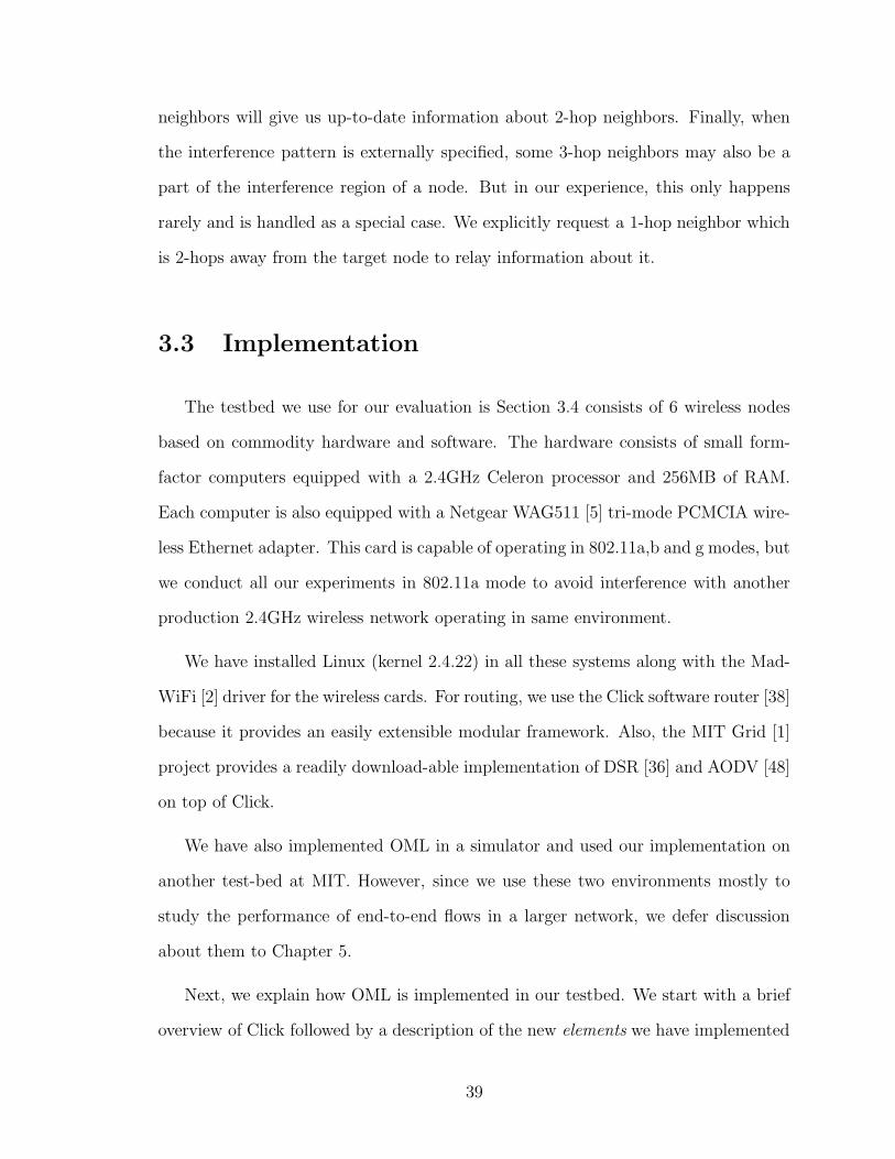
neighbors will give us up-to-date information about 2-hop neighbors. Finally, when
the interference pattern is externally specified, some 3-hop neighbors may also be a
part of the interference region of a node. But in our experience, this only happens
rarely and is handled as a special case. We explicitly request a 1-hop neighbor which
is 2-hops away from the target node to relay information about it.
3.3 Implementation
The testbed we use for our evaluation is Section 3.4 consists of 6 wireless nodes
based on commodity hardware and software. The hardware consists of small form-
factor computers equipped with a 2.4GHz Celeron processor and 256MB of RAM.
Each computer is also equipped with a Netgear WAG511 [5] tri-mode PCMCIA wire-
less Ethernet adapter. This card is capable of operating in 802.11a,b and g modes, but
we conduct all our experiments in 802.11a mode to avoid interference with another
production 2.4GHz wireless network operating in same environment.
We have installed Linux (kernel 2.4.22) in all these systems along with the Mad-
WiFi [2] driver for the wireless cards. For routing, we use the Click software router [38]
because it provides an easily extensible modular framework. Also, the MIT Grid [1]
project provides a readily download-able implementation of DSR [36] and AODV [48]
on top of Click.
We have also implemented OML in a simulator and used our implementation on
another test-bed at MIT. However, since we use these two environments mostly to
study the performance of end-to-end flows in a larger network, we defer discussion
about them to Chapter 5.
Next, we explain how OML is implemented in our testbed. We start with a brief
overview of Click followed by a description of the new elements we have implemented
39

in Click. Finally, we show how these elements are used in a typical multi-hop wireless
router configuration.
3.3.1 Overview of Click
The Click Modular Router[38] is a software architecture developed at MIT for
building routers. We only cover the essentials required to understand our implemen-
tation of OML. For further details, we refer the reader to [38].
Elements are the building block of a Click router. Elements typically perform
some simple packet processing task and are implemented as a C++ class. Packets
flow in and out of elements through ports. A router is a directed graph of elements
connected through their ports using push or pull connections. In a push connection,
data flow is initiated by the upstream element (e.g., input to a queue), whereas in a
pull connection, the downstream element is the initiator (e.g., output from a queue).
The configuration for the router is a directed graph with elements at the vertices and
packets flowing along the edges and is specified through a simple text file.
In addition to ports which deal with the data flow, elements can also implement
handlers. Handlers are used to implement control operations outside the data flow,
e.g., a queue might export a handler that reports the current length of the queue.
A downstream element that implements a scheduling algorithm can then use this
handler to decide which input to dequeue from.
3.3.2 OML Elements in Click
The majority of OML functionality is implemented using the two elements, TimeS-
lotEnforcer and ContentionResolver. TimeSlotEnforcer is responsible for making sure
that send requests are issued only in the allowed time slots. The length of a slot (l)
40
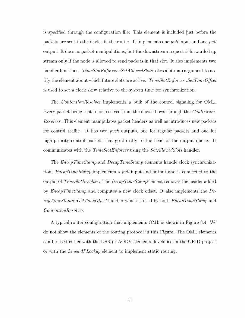
is specified through the configuration file. This element is included just before the
packets are sent to the device in the router. It implements one pull input and one pull
output. It does no packet manipulations, but the downstream request is forwarded up
stream only if the node is allowed to send packets in that slot. It also implements two
handler functions. TimeSlotEnforcer::SetAllowedSlots takes a bitmap argument to no-
tify the element about which future slots are active. TimeSlotEnforcer::SetTimeOffset
is used to set a clock skew relative to the system time for synchronization.
The ContentionResolver implements a bulk of the control signaling for OML.
Every packet being sent to or received from the device flows through the Contention-
Resolver. This element manipulates packet headers as well as introduces new packets
for control traffic. It has two push outputs, one for regular packets and one for
high-priority control packets that go directly to the head of the output queue. It
communicates with the TimeSlotEnforcer using the SetAllowedSlots handler.
The EncapTimeStamp and DecapTimeStamp elements handle clock synchroniza-
tion. EncapTimeStamp implements a pull input and output and is connected to the
output of TimeSlotResolver. The DecapTimeStampelement removes the header added
by EncapTimeStamp and computes a new clock offset. It also implements the De-
capTimeStamp::GetTimeOffset handler which is used by both EncapTimeStamp and
ContentionResolver.
A typical router configuration that implements OML is shown in Figure 3.4. We
do not show the elements of the routing protocol in this Figure. The OML elements
can be used either with the DSR or AODV elements developed in the GRID project
or with the LinearIPLookup element to implement static routing.
41
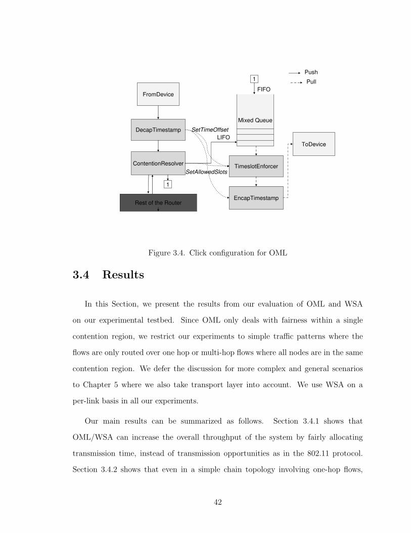
Figure 3.4. Click configuration for OML
3.4 Results
In this Section, we present the results from our evaluation of OML and WSA
on our experimental testbed. Since OML only deals with fairness within a single
contention region, we restrict our experiments to simple traffic patterns where the
flows are only routed over one hop or multi-hop flows where all nodes are in the same
contention region. We defer the discussion for more complex and general scenarios
to Chapter 5 where we also take transport layer into account. We use WSA on a
per-link basis in all our experiments.
Our main results can be summarized as follows. Section 3.4.1 shows that
OML/WSA can increase the overall throughput of the system by fairly allocating
transmission time, instead of transmission opportunities as in the 802.11 protocol.
Section 3.4.2 shows that even in a simple chain topology involving one-hop flows,
42

802.11 can cause a significant number of TCP flows to experience starvation, while
OML can avoid this. Section 3.4.3 shows that, as expected, the starvation problem
under 802.11 is even worse in the case of multi-hop routing, but OML can help in
this case also. In Section 3.4.4, we evaluate the allocation accuracy of WSA using a
simple scenario. Finally, in Section 3.4.5, we show that OML is also effective in the
presence of short flows.
To quantify the fairness of the system, we use the metric defined by Chiu and Jain
in [16]. Consider a system with M flows, with weights w1, w2, . . . , wM , each receiving
a throughput x1, x2, . . . , xM . The fairness index F is defined as
F =(∑
i xi/wi)2
M∑
i x2i /w
2i
Note that F = 1 when each flow’s throughput is exactly in proportion to its
weight, and F = 1/M when only one flow receives the entire throughput.
3.4.1 Heterogeneous data rates
In this experiment, we reconsider the scenario described in Section 3.1.1.2 where
two nodes are simultaneously sending one flow each to the access point (unlike the rest
of our experiments, we use the infrastructure mode for this one). One node operates
at 54 Mbps, and the other node operates at rates ranging from 6 to 54 Mbps. We
use the WSA algorithm to allocate the bandwidth, with each node having the same
weight. This leads to each node receiving an equal channel-access time, rather than
an equal number of transmission opportunities as in 802.11. Note that this allocation
implements the temporal-sharing policy as proposed in [57]. Figure 3.5 shows the
throughputs of both flows. The two flows receive throughputs approximately propor-
43

Figure 3.5. 802.11 throughput in the presence of heterogeneous data rate sendersusing OML
tional to the rates they are operating at, and the total system throughput does not
drop by as much (compared to 802.11) when the second node is operating at 6 Mbps.
3.4.2 Chain topology
In this experiment, we configure our testbed as a five-hop chain, and pick two
random links in this chain. Figure 3.6 shows the CDF of the flows’ throughputs along
these links over 50 trials. We consider four scenarios: (a) the flows are started one
at a time (b) the flows are started at the same time (i.e., simultaneous flows) using
baseline 802.11 (without OML), (c) simultaneous flows using OML assuming one-
hop interference (k = 1), and (d) simultaneous flows using OML assuming two-hop
interference (k = 2). When using OML each flow is assigned a unit weight.
As expected, in scenario (a) when only one flow is active, the flows get very good
throughput. In 96% of the cases the throughput is greater than 4Mbps. However,
44
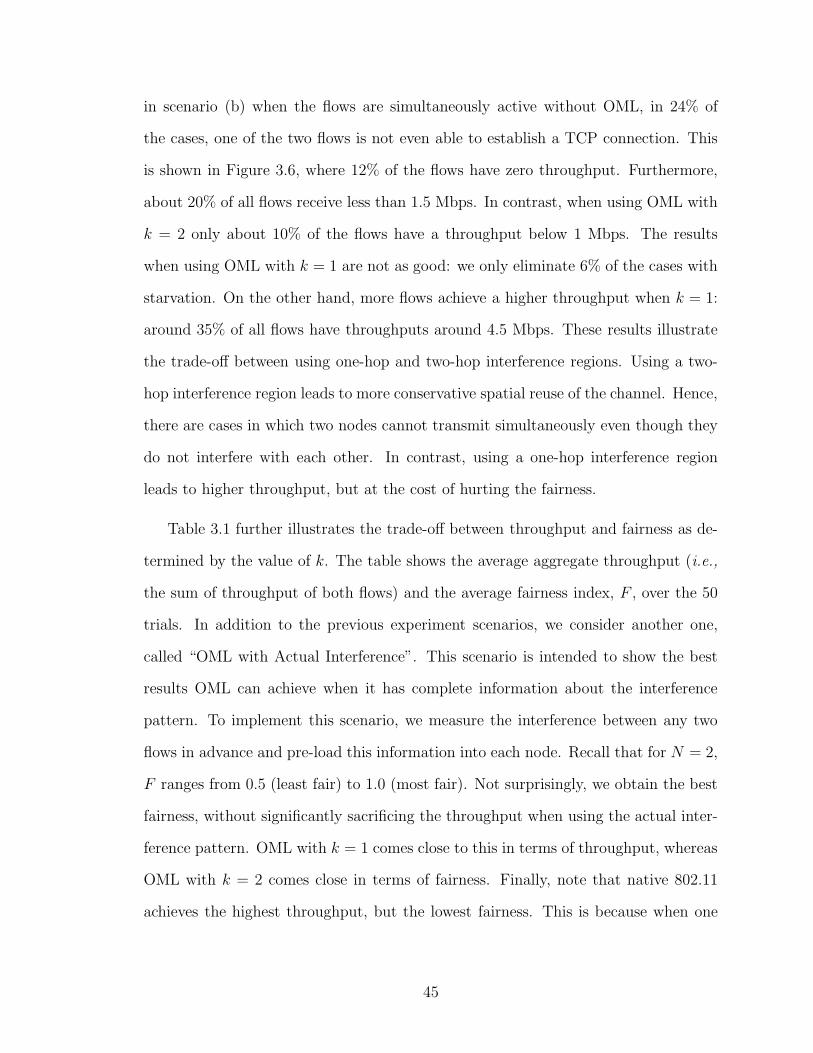
in scenario (b) when the flows are simultaneously active without OML, in 24% of
the cases, one of the two flows is not even able to establish a TCP connection. This
is shown in Figure 3.6, where 12% of the flows have zero throughput. Furthermore,
about 20% of all flows receive less than 1.5 Mbps. In contrast, when using OML with
k = 2 only about 10% of the flows have a throughput below 1 Mbps. The results
when using OML with k = 1 are not as good: we only eliminate 6% of the cases with
starvation. On the other hand, more flows achieve a higher throughput when k = 1:
around 35% of all flows have throughputs around 4.5 Mbps. These results illustrate
the trade-off between using one-hop and two-hop interference regions. Using a two-
hop interference region leads to more conservative spatial reuse of the channel. Hence,
there are cases in which two nodes cannot transmit simultaneously even though they
do not interfere with each other. In contrast, using a one-hop interference region
leads to higher throughput, but at the cost of hurting the fairness.
Table 3.1 further illustrates the trade-off between throughput and fairness as de-
termined by the value of k. The table shows the average aggregate throughput (i.e.,
the sum of throughput of both flows) and the average fairness index, F , over the 50
trials. In addition to the previous experiment scenarios, we consider another one,
called “OML with Actual Interference”. This scenario is intended to show the best
results OML can achieve when it has complete information about the interference
pattern. To implement this scenario, we measure the interference between any two
flows in advance and pre-load this information into each node. Recall that for N = 2,
F ranges from 0.5 (least fair) to 1.0 (most fair). Not surprisingly, we obtain the best
fairness, without significantly sacrificing the throughput when using the actual inter-
ference pattern. OML with k = 1 comes close to this in terms of throughput, whereas
OML with k = 2 comes close in terms of fairness. Finally, note that native 802.11
achieves the highest throughput, but the lowest fairness. This is because when one
45
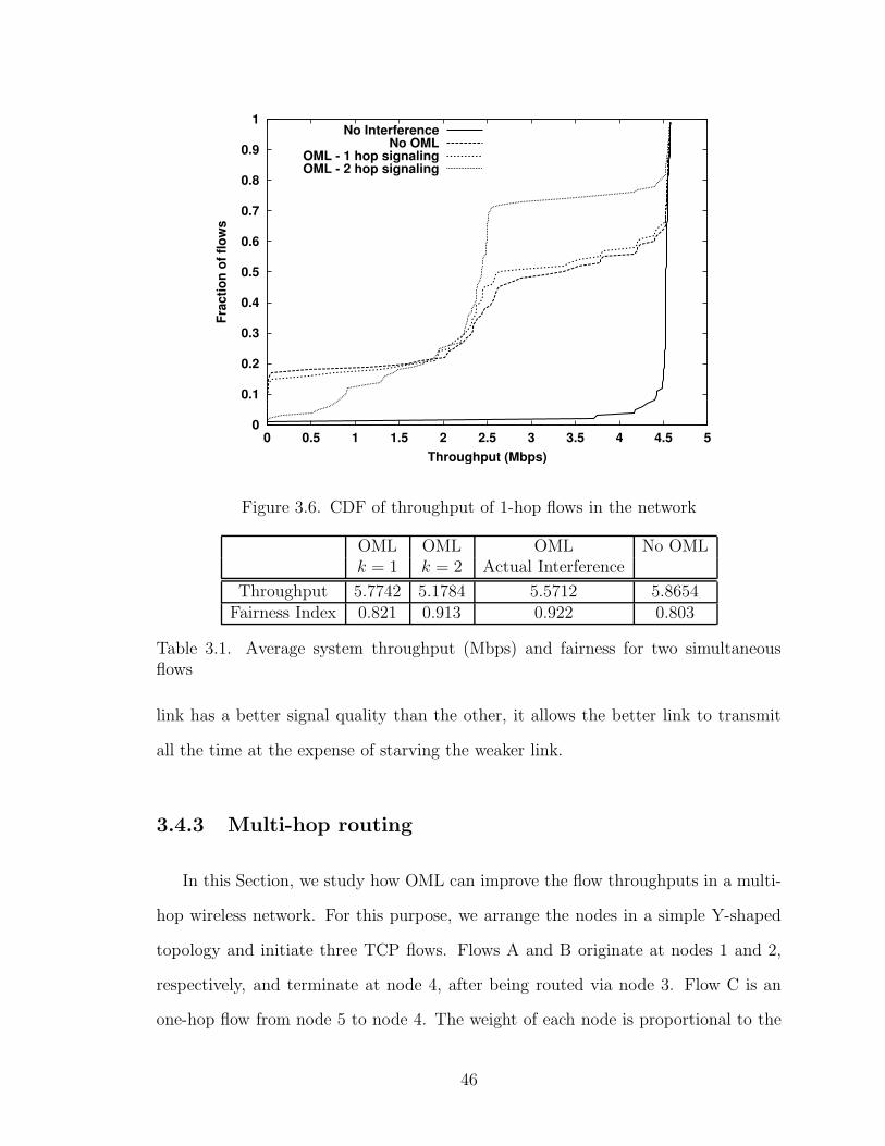
0
0.1
0.2
0.3
0.4
0.5
0.6
0.7
0.8
0.9
1
0 0.5 1 1.5 2 2.5 3 3.5 4 4.5 5
Frac
tion
of fl
ows
Throughput (Mbps)
No InterferenceNo OML
OML - 1 hop signalingOML - 2 hop signaling
Figure 3.6. CDF of throughput of 1-hop flows in the network
OML OML OML No OMLk = 1 k = 2 Actual Interference
Throughput 5.7742 5.1784 5.5712 5.8654Fairness Index 0.821 0.913 0.922 0.803
Table 3.1. Average system throughput (Mbps) and fairness for two simultaneousflows
link has a better signal quality than the other, it allows the better link to transmit
all the time at the expense of starving the weaker link.
3.4.3 Multi-hop routing
In this Section, we study how OML can improve the flow throughputs in a multi-
hop wireless network. For this purpose, we arrange the nodes in a simple Y-shaped
topology and initiate three TCP flows. Flows A and B originate at nodes 1 and 2,
respectively, and terminate at node 4, after being routed via node 3. Flow C is an
one-hop flow from node 5 to node 4. The weight of each node is proportional to the
46
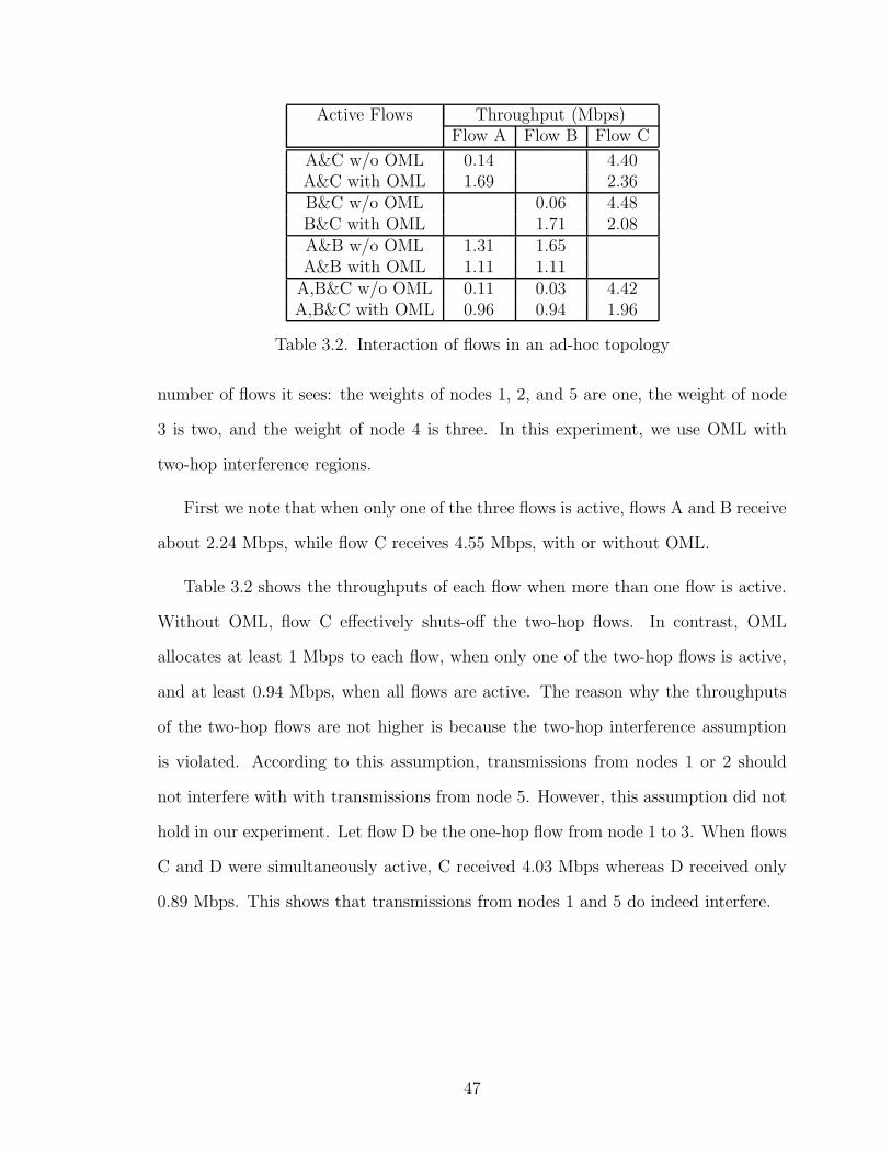
Active Flows Throughput (Mbps)Flow A Flow B Flow C
A&C w/o OML 0.14 4.40A&C with OML 1.69 2.36B&C w/o OML 0.06 4.48B&C with OML 1.71 2.08A&B w/o OML 1.31 1.65A&B with OML 1.11 1.11
A,B&C w/o OML 0.11 0.03 4.42A,B&C with OML 0.96 0.94 1.96
Table 3.2. Interaction of flows in an ad-hoc topology
number of flows it sees: the weights of nodes 1, 2, and 5 are one, the weight of node
3 is two, and the weight of node 4 is three. In this experiment, we use OML with
two-hop interference regions.
First we note that when only one of the three flows is active, flows A and B receive
about 2.24 Mbps, while flow C receives 4.55 Mbps, with or without OML.
Table 3.2 shows the throughputs of each flow when more than one flow is active.
Without OML, flow C effectively shuts-off the two-hop flows. In contrast, OML
allocates at least 1 Mbps to each flow, when only one of the two-hop flows is active,
and at least 0.94 Mbps, when all flows are active. The reason why the throughputs
of the two-hop flows are not higher is because the two-hop interference assumption
is violated. According to this assumption, transmissions from nodes 1 or 2 should
not interfere with with transmissions from node 5. However, this assumption did not
hold in our experiment. Let flow D be the one-hop flow from node 1 to 3. When flows
C and D were simultaneously active, C received 4.03 Mbps whereas D received only
0.89 Mbps. This shows that transmissions from nodes 1 and 5 do indeed interfere.
47

Weight of A 1 1 1 1Throughput of A 2.26 1.48 1.36 0.92
Weight of B 1 2 3 4Throughput of B 2.20 2.97 3.06 3.64
Table 3.3. Throughput received by senders with different weights
Size of Flow 16k 32k 64 128k 256k
Time w/o OML (s) 0.06 0.12 0.23 0.46 0.93Time with OML (s) 0.11 0.17 0.29 0.50 0.97
Table 3.4. Transfer time of a short flow in the presence of a long flow
3.4.4 Weighted allocation
In this experiment, we evaluate the accuracy of WSA, and thus its ability to
provide per-node service differentiation by setting the node weights. We consider two
nodes A and B that send a TCP flow each to a third node C. We set the weight of
node A to 1, and assign a weight ranging from 1 to 4 to node B. Table 3.3 shows
the throughput achieved by the nodes for each combination of weights. As expected,
the ratio of throughputs obtained by the two nodes tracks the ratio of their weights
closely.
3.4.5 Short Flows
Due to the additional delay caused by queueing packets while waiting to obtain a
time-slot, OML can impose a significant overhead on short TCP flows. To quantify
this overhead, we conduct the following experiment. We start two simultaneous one
hop flows, both terminating at the same node; the first flow is a long-lived TCP flow,
while the second is a short TCP flow of varying size. Table 3.4 shows the transfer
time of the second flow as a function of its size. As we can see, the effect of OML
translates to a fixed time overhead, usually less than 60ms. As the size of the flow
increases, the degradation reduces. For flows larger than 100 kilobytes, the resulting
48

throughput degradation is less than 10%. This fixed overhead is simply the time it
takes for the TCP slow start to ramp up under OML. Though we expect this overhead
to be higher for longer (more than one hop) flows, the steady state throughput of such
flows is also lower.3 Thus, we expect the relative overhead to be similar.
3Flows that traverse multiple hops in wireless networks are limited to a lower throughput due tothe contention between the different hops of the same flow.
49

Chapter 4
Detecting Interference using
Passive Measurements
As mentioned earlier, OML, as well as a lot of other applications require infor-
mation about which links interfere with each other in a wireless network. In this
Chapter, we develop an algorithm that can detect interference as it happens during
the normal operation of the network. We start with an overview of our approach in
Section 4.1, followed by a presentation of the details of our algorithm in Section 4.2.
Next, we explain our evaluation methodology by describing our simulation and test-
bed environments in Section 4.3. Finally, we presents the results from our evaluation
in Section 4.4.
4.1 Our Approach
Our approach is motivated by the success of passive measurement techniques in
wired networks [35, 27]. Passive measurements provide a non-intrusive way to obtain
certain network-level performance metrics by studying the behavior of existing traffic.
50
In our system, the additional overhead is limited to a small header in each packet
used to broadcast control information in a local neighborhood.
One of the advantages of using passive measurements is that even though there
may be a large number of links in a network (which can take a long time to measure
exhaustively), a lot of applications e.g., scheduling and resource allocation only need
interference information for the links that are currently in use. In practice, we found
that for most traffic patterns, this subset of links tends to be much smaller for the
following two reasons. Firstly, because of the limited channel capacity, we can only
have a limited number of flows simultaneously sending data at any given time. Sec-
ondly, of the available links, the routing protocol tends to prefer certain links over
others. However, active measurement based approaches may be forced to measure the
entire network even in this case because there is no way of knowing which links are
going to be used until a flow actually starts sending data on that link. By this time,
it is too late to do start measurements using the same link without severely hurting
the performance of that flow. On the other hand, since passive measurements use
existing traffic, they automatically detect interference for useful links only.
Note that some applications may indeed need interference information for all links
in the network. In such cases, it may be possible to supplement passive measurements
with active measurements during periods of lean user traffic. However, such extensions
are outside the scope of this paper. As a start, we have chosen to focus on time-slot
based scheduling; this application only requires information about links that carry
traffic.
To detect interference through passive measurements, we have to keep track of
the following information.
• Exactly which links are sending data during any given time period.
51

• The throughput on each of these links during this period.
As mentioned in Chapter 3, OML divides time into equal size slots and keeps
track of which nodes are transmitting in each slot; thus using OML automatically
takes care of the first requirement. For the second requirement, we made a simple
change to OML to log the number of successful packet transmissions during every
time slot at the sender of each link.
Once we detect interference between a pair of links, we feed that information back
into OML, which in turn will ensure that these links are not allowed to transmit in the
same time slot subsequently. Previously (in Chapter 3) we used very simple hop-based
heuristics to approximate the interference pattern used by OML. Here, we modify
this in the following way. During cold start, we do not have sufficient information to
confidently state which links interfere. So, when the network starts up, we trigger
an exploration process by allowing OML to schedule some interfering links in the
same time slot. Over time, we detect interference based on the performance of these
links. Once we are sure that we can reduce interference and improve performance
by preventing a pair of links from transmitting at the same time, we augment the
interference pattern used by OML with this new information.
Note that though our current implementation uses OML, our algorithm can work
on top any TDMA MAC that keeps track of which nodes are transmitting in each
time slot. However, we believe that the two layer MAC architecture of OML provides
the following additional benefits.
• We are protected by the underlying 802.11 MAC layer while the interference
pattern is being probed by deliberately scheduling interfering links in the same
time slot.
• Most readily available hardware (including those based on newer standards such
52

as 802.11n) already implement some form of a CSMA MAC. In most cases, this
layer cannot be disabled without hardware modifications.
• Even if designing and building custom hardware is possible, we believe that
carrier sensing before transmission is a good idea for radios operating in the
ISM bands. There will always be other hardware that could potentially interfere
but do not follow the rules of the particular TDMA MAC in use.
4.2 Algorithm
We now present the design of our algorithm to detect interference using passive
measurements. For ease of explanation, we initially describe a centralized version of it
assuming global visibility of the entire network (Section 4.2.2). We then show how it
can be implemented in a distributed manner in Section 4.2.3. But before we delve into
the details, we state our assumptions and present some definitions in Section 4.2.1.
4.2.1 Definitions and Assumptions
In this Section, we explain exactly what we mean by interference in the context
of this algorithm. Earlier work in this area has used different ways of specifying the
interference pattern of a wireless network [34, 46]. In the most general case, we have
to specify exactly what happens when each subset of links is active. However, in this
work, we use a pair-wise, binary model as used in [34].
The pair-wise assumption means that we can specify the entire interference pattern
by only specifying how any given pair of links interfere. In other words, there are
no three links A, B and C such that there is interference when all three of them are
active, but no interference when any subset of only two links is active. To predict
53

interference between k links for k ≥ 3, we only have to check if any one of the(
k2
)
pairs of links contained in this set interfere.
Also, for simplicity, we define interference as a binary phenomenon. More formally,
given two links A and B, with throughput tA and tB in isolation, we measure their
throughput when they are simultaneously active as tA/AB and tB/AB respectively. We
say that A and B interfere if and only if tA/AB < αtA or tB/AB < αtB. The parameter
α lies in the range 0 < α < 1 and is chosen by the application.
The pair-wise binary assumption allows us to represent the interference in a net-
work through a simple interference graph G = (L, E). The set L contains a vertex
corresponding to each link in the network. We have an edge between two links A
and B if and only if they interfere as per our previous definition of interference.1
Figure 4.1 shows a simple network topology with five links labeled as A through E.
For clarity, we do not consider the rest of the links (shown with dotted lines). Links
A, B and D interfere with C. In addition, links A and B interfere with each other,
and E interferes with D. The resulting interference graph for these five links is shown
to the right.
4.2.2 Centralized Algorithm
In this Section, we assume that we have information about the entire network
at a centralized location. Since we are operating on top a time-slot based MAC,
we assume that we have history available for all time slots between startTime and
endTime. This information is stored in the array shi of type SlotHistoryInfo. Each
SlotHistoryInfo record has information about every link in the network in a particular
time slot. shi[t].link[i].active indicates if the link i was transmitting during time slot
1We use the terms nodes and links when we refer to the network topology graph, and the termsvertex and edge with respect to other graphs. For example, links are actually vertices in the inter-ference graph.
54
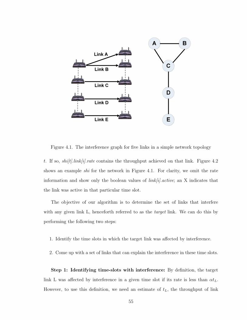
Link A
B
C
A
D
Link B
Link C
Link D
Link E E
Figure 4.1. The interference graph for five links in a simple network topology
t. If so, shi[t].link[i].rate contains the throughput achieved on that link. Figure 4.2
shows an example shi for the network in Figure 4.1. For clarity, we omit the rate
information and show only the boolean values of link[i].active; an X indicates that
the link was active in that particular time slot.
The objective of our algorithm is to determine the set of links that interfere
with any given link L, henceforth referred to as the target link. We can do this by
performing the following two steps:
1. Identify the time slots in which the target link was affected by interference.
2. Come up with a set of links that can explain the interference in these time slots.
Step 1: Identifying time-slots with interference: By definition, the target
link L was affected by interference in a given time slot if its rate is less than αtL.
However, to use this definition, we need an estimate of tL, the throughput of link
55
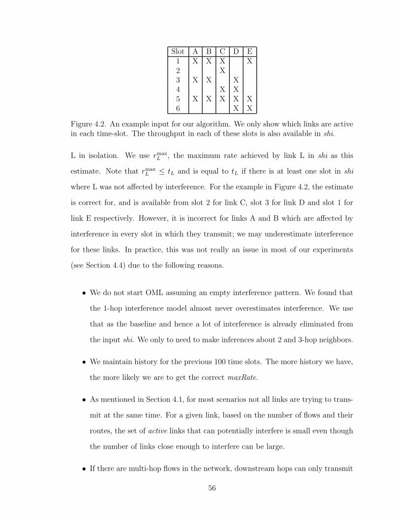
Slot A B C D E1 X X X X2 X3 X X X4 X X5 X X X X X6 X X
Figure 4.2. An example input for our algorithm. We only show which links are activein each time-slot. The throughput in each of these slots is also available in shi.
L in isolation. We use rmaxL , the maximum rate achieved by link L in shi as this
estimate. Note that rmaxL ≤ tL and is equal to tL if there is at least one slot in shi
where L was not affected by interference. For the example in Figure 4.2, the estimate
is correct for, and is available from slot 2 for link C, slot 3 for link D and slot 1 for
link E respectively. However, it is incorrect for links A and B which are affected by
interference in every slot in which they transmit; we may underestimate interference
for these links. In practice, this was not really an issue in most of our experiments
(see Section 4.4) due to the following reasons.
• We do not start OML assuming an empty interference pattern. We found that
the 1-hop interference model almost never overestimates interference. We use
that as the baseline and hence a lot of interference is already eliminated from
the input shi. We only to need to make inferences about 2 and 3-hop neighbors.
• We maintain history for the previous 100 time slots. The more history we have,
the more likely we are to get the correct maxRate.
• As mentioned in Section 4.1, for most scenarios not all links are trying to trans-
mit at the same time. For a given link, based on the number of flows and their
routes, the set of active links that can potentially interfere is small even though
the number of links close enough to interfere can be large.
• If there are multi-hop flows in the network, downstream hops can only transmit
56

when they have already received data from the upstream hops. Also, upstream
hops depend on the TCP congestion control algorithm (window size and the
reception of ACKs) to be able to send data. This means that even for links that
are on the route of an active flow, they are not trying to transmit data at all
times.
Note that even if this turns out to be a problem for some network scenario, a simple
fix is possible. We can periodically, say every 5 minutes, schedule a slot (for each link)
where we explicitly disallow all links we suspect might interfere from transmitting.
We can then store the obtained throughput as the maximum rate for that link.
Step 2: Identifying the links which interfere: We now know that at least
one interfering link was active in each time slot identified in the previous step. In
order to come up with a set that satisfies this property, we first construct a bipartite
graph, intGraph as follows. The vertex set of the graph is given by (V1 + V2) where
V1 = L, the set of links in the network and V2 = T , the set of time slots in shi. We
connect a link M to a time slot t if and only if:
1. The target link L was affected by interference in time slot t
2. Link M was active in time slot t.
Figure 4.3(a) shows the graph constructed with link D as the target using the shi
in Figure 4.2.
Based on our construction of intGraph, we know that every vertex of non-zero
degree in V2 has to be adjacent to at least one link that interferes with L. However,
there can be many subsets of V1 that satisfy this property. Since it is easier to identify
links that do not cause interference, we start by doing that first. For example, in slot
3, links A and B are both active and yet D was not affected by interference. Therefore,
57

A
C
B
1
2
3
4
5
6E
D
(a)
A
C
B
1
2
3
4
5
6E
D
(b)
A
C
B
1
2
3
4
5
6E
D
(c)
A
C
B
1
2
3
4
5
6E
D
(d)
Target Link
I nterf ering Link
D el eted V ertexD el eted E d ge
Figure 4.3. The graphs constructed by GetInterferingLinks(D) for the network inFigure 4.1 using the shi in Figure 4.2. We initially start with graph (a), which yields(b) after the clean-up phase. We then detect links C and E as interfering links overtwo iterations; the corresponding graphs are shown in (c) and (d).
58

we can clean up the graph by removing the vertices corresponding to A and B (see
Figure 4.3(b)). More formally, we identify all links N such that (a) both L and N are
active and (b) L achieves a rate of at least βtL, and remove such links from V1 in the
clean up phase. The parameter β is lies in the range α < β < 1. Choosing a β that
is not exactly equal to α or 1 helps guard against small variations in performance of
links caused by external factors.
While the clean up phase helps reduce the ambiguity in choosing an appropriate
subset of V1, there is no guarantee that all ambiguity is eliminated. At this point, we
have to take a guess and pick some subset that helps explain all interference. We do
this by repeating the following two steps until there are no more edges in intGraph.
1. Pick a vertex V of non-zero degree in V1 and add it to the set of interfering
links.
2. Remove all vertices that are adjacent to V. Note that the removal of a vertex
from a graph also results in the removal of all edges that are incident on that
vertex.
The second step ensures that we only add a new link to the set if it accounts
for interference that is not already explained by links chosen earlier. Note that even
if we underestimate interference, we are likely to see it again in the near future.
Therefore we believe that a conservative policy which affects performance by taking
slightly longer to detect interference is preferable over an aggressive policy which
makes a lot of incorrect inferences. This process takes two iterations for the graph in
Figure 4.3(b). Link C is chosen in the first iteration which results in the removal of
nodes 4 and 5 (Figure 4.3(c)). Link E is chosen in the next step which results in a
graph with no links (Part (d) of the same Figure).
We still haven’t explained how we pick a vertex from V1 in each iteration. Intu-
59

itively, we want to pick links that are more likely to have caused interference at target
link first. A simple heuristic is to pick the node with the highest degree in V1 at each
step; this helps explain interference in the most number of time slots. However, this
does not account for the fact that interference is some slots is easier to disambiguate
than in others. For example, the interference in slot 5 could have been caused by
either link C or E, but the interference in slots 4 and 6 can only be explained by one
link. We account for this factor by using a weighted degree heuristic. The weight of
an edge (v1, v2) where v1 ∈ V1 and v2 ∈ V2 is defined as the reciprocal of the degree of
v2. Thus, the edges incident on slot 5 have a degree 1
2in Figure 4.3(b). The weighted
degree of a vertex in V1 is the sum of the weights of the edges incident on it.
Figure 4.4 gives the complete pseudocode for our algorithm. More specifically,
the function GetInterferingLinks() returns the list of links that interfere with any
given link using shi as input. The first for loop (lines 5 to 7) computes maxRate
as an estimate for tL. The second for loop (lines 11 to 20) constructs the bipartite
graph which is represented as an array of adjacency lists in intGraph. In order to the
implement the weighted degree heuristic, we also create the array numIntLinks which
keeps track of the degree of vertices in V2. The completes Step 1 of the algorithm.
The next for loop (lines 22 to 31) implements the clean up phase followed by the
last while loop (lines 33 to 59) which removes vertices and nodes from the graph
according to the weighted degree heuristic.
4.2.3 Distributed Algorithm
The key idea behind our distributed implementation is that each node is respon-
sible for deciding which other links are interfering with its transmissions. In order to
do this, each node executes the following steps:
1. Gather data about all other links it thinks might interfere with its transmissions.
60
2. Run GetInterferingLinks locally with this information.
3. Notify other nodes once it concludes that they interfere with its transmissions.
This is required because interference sometimes only affects the performance of
one of the two links. But OML needs the information at both senders to ensure
that they don’t transmit at the same time.
In order to stay current in a dynamic network, we have to repeat these steps
periodically to learn new information. The data gathered in step (1) is kept up-to-
date by continuously flooding information about recent timeslots piggybacked on the
headers of data packets. This mechanism is described in detail in Section 4.2.3.1.
Step (2) can be significantly optimized by saving the constructed intGraph between
calls to GetInterferingLinks. In each call, we first discard all edges and vertices where
the time slot is less than the new startTime. To add new links, we only have to
process shi between the previous endTime and the current one. Finally, in step (3)
we only have to notify neighbors that haven’t already been notified during previous
calls to GetInterferingLinks.
4.2.3.1 Scoped flooding of link information
The first observation we make regarding GetInterferingLinks is that at any given
node, we only need time-slot level information about other links that could potentially
interfere with transmissions originating at that node; the algorithm does not require
information about links that are “far away” in the network. In practice, we found
three network hops to be a very good upper bound on the interference range of a
given link. Thus at every node we need information about links that are within three
network hops of this node and the time slots in which these links were active. Instead
of explicitly flooding this information, we will now explain how we can achieve a much
lower overhead by using packet snooping and piggybacking techniques.
61
Since OML enables promiscuous receptions at every node, we automatically get
information about links that are one hop away. If sender is one hop away, we can
snoop on all data transmissions on that link. On the other hand, if only the receiver
is one-hop away, we can use the link layer ACKs to determine when data was being
sent on that link. In order to gather information about 2-hop and 3-hop neighbors,
we piggyback this data in the headers of data transmissions from each node. For
each link, the time-slots in which it was active are represented through a simple
bitmap that uses only 1-bit for each time-slot. We include information about every
1-hop neighbor in each packet; this ensures that each node has relatively up-to-date
data about its 2-hop neighbors by listening to all transmissions in promiscuous mode.
However, to save space in the header, we only include information about selected
2-hop neighbors (chosen at random and changed periodically). We found this to be
an acceptable trade-off for two reasons
• For each 3-hop neighbor n, there is typically more than one immediate neighbor
that can reach n over 2-hops. We will receive information about n as long as it
is chosen by any one of these neighbors.
• Even if the node is not chosen by any of these 1-hop neighbors, it is likely
to be chosen later when one of them updates their selection. Thus, it might
take longer to infer interference from 3-hop neighbors. In our experiments,
interference from 3-hop neighbors was very rare and did not significantly affect
performance.
Our implementation typically adds 40 to 60 bytes of overhead in the header of
each packet. It may be possible to further optimize this using header compression
techniques [40, 64]. A lot of our header overhead consists of bitmaps that indicate
when each link was active; these bitmaps tend to be sparse since only one of several
interfering links can be active at any given time. We can potentially save more
62

space by using bloom filters [43] or other advanced techniques [44] designed for such
bitmaps. The implementation of such techniques, however, is outside the scope of
this work.
4.2.3.2 Removing Stale Inferences
We use a very simple time-out based mechanism to ensure that we expire stale
inferences as the network changes. We assume that the inferences made by GetInter-
feringLinks are valid only for a maximum of one hour. This is a very conservative
assumption; when the nodes are not mobile, the interference changed for only 8% of
the link pairs when measured five days apart [46]. But it works well in practice because
most inferences take less than one minute in our experiments(see Section 4.4). We
randomize the expiration timer between 45 and 60 minutes to avoid synchronization
where a large number inferred interferences become invalid at the same time.
The above mechanism works well when nodes are stationary and channel con-
ditions are static. However, if the network (nodes move) or the channel conditions
change (a microwave oven is turned on, obstacles such as furniture are moved etc.)
we need a mechanism to detect this change and react sooner than an hour.2 We use
the throughput of a link in the absence of any interference as an indicator for its sta-
bility. This throughput is calculated as maxRate in GetInterferingLinks. If maxRate
changes by more that 50% from the time a particular inference was made, we do not
consider it to be valid any longer. We immediately expire this information by sending
a explicit message to the other senders.
2Our scheme may not be suitable for networks where the mobility is very high. In this case, wemay be unable to detect interference quickly enough for it to be useful. Even though we do detectchanges pretty quickly, we require that the changes are not too frequent.
63
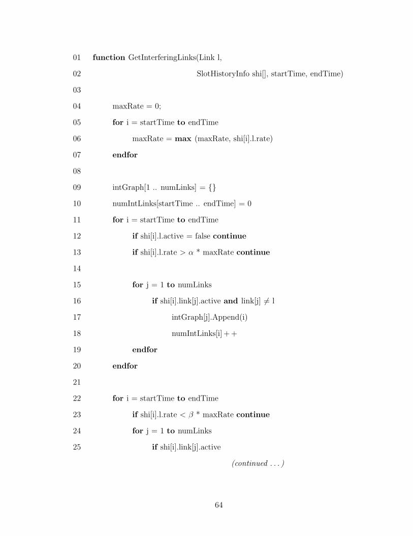
01 function GetInterferingLinks(Link l,
02 SlotHistoryInfo shi[], startTime, endTime)
03
04 maxRate = 0;
05 for i = startTime to endTime
06 maxRate = max (maxRate, shi[i].l.rate)
07 endfor
08
09 intGraph[1 .. numLinks] = {}
10 numIntLinks[startTime .. endTime] = 0
11 for i = startTime to endTime
12 if shi[i].l.active = false continue
13 if shi[i].l.rate > α * maxRate continue
14
15 for j = 1 to numLinks
16 if shi[i].link[j].active and link[j] 6= l
17 intGraph[j].Append(i)
18 numIntLinks[i] + +
19 endfor
20 endfor
21
22 for i = startTime to endTime
23 if shi[i].l.rate < β * maxRate continue
24 for j = 1 to numLinks
25 if shi[i].link[j].active
(continued . . . )
64
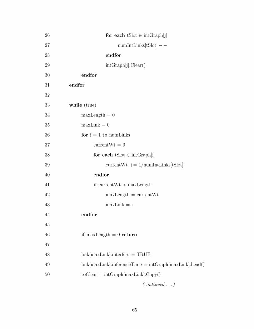
26 for each tSlot ∈ intGraph[j]
27 numIntLinks[tSlot]−−
28 endfor
29 intGraph[j].Clear()
30 endfor
31 endfor
32
33 while (true)
34 maxLength = 0
35 maxLink = 0
36 for i = 1 to numLinks
37 currentWt = 0
38 for each tSlot ∈ intGraph[i]
39 currentWt += 1/numIntLinks[tSlot]
40 endfor
41 if currentWt > maxLength
42 maxLength = currentWt
43 maxLink = i
44 endfor
45
46 if maxLength = 0 return
47
48 link[maxLink].interfere = TRUE
49 link[maxLink].inferenceTime = intGraph[maxLink].head()
50 toClear = intGraph[maxLink].Copy()
(continued . . . )
65

51
52 for i = 1 to numLinks
53 for j = 1 to length(toClear)
54 intGraph[i].Remove(toClear[j])
55 endfor
56 endfor
57
58 intGraph[maxLink].Clear()
59 endwhile
60
61 endfunction
Figure 4.4. The pseudocode for the centralized algorithm to get the list of links thatinterfere with a given link
66

4.3 Evaluation Methodology
In order to evaluate our algorithm, we have implemented it in a test-bed, which
we describe in Section 4.3.2, and in a simulator which we describe below.
4.3.1 Simulation
Our simulator is based on ns2 [6], an event-based packet level simulator and it’s
wireless extensions developed at the Carnegie Mellon University. Even though our
ultimate goal was to implement our algorithms in a real test-bed, we found a simulator
to be useful for a number of reasons. Firstly, unlike a test-bed, the simulator allows
us to make changes and perform experiments very quickly - this was very useful while
we were designing our algorithm. Secondly, the simulator allows to us change the
characteristics of the antenna and the wireless medium very easily.
4.3.1.1 Interference pattern in simulation
In order to stress our algorithm, we have implemented two new signal propaga-
tion models in ns2. The first model is a purely synthetic model that generates an
interference pattern based on a certain probability of interference at each distance.
The second model simulates the gain pattern of a directional antenna. These models
are described below.
Hop-based interference: In this model, for any two nodes A and B, they can
either:
1. Communicate with each other.
2. Carrier sense each others transmissions.
3. Do not interfere.
67

We say that A and B interfere if they are in categories (1) or (2). To decide
the relationship between a given pair of nodes, we do the following at the start of
each simulation. First, we set the communication range to 250m and compute the
distance between them in terms of the number of hops. By definition, two nodes can
communicate and if only if they are 1-hop away. For nodes separated by two hops,
there is a 60% chance that they are within carrier sense range of each other and a 40%
chance they do not interfere. At three hops, there is a 40% chance that nodes can
carrier sense each other, and nodes that are more than 3 hops away never interfere.
Based on this model, to determine if two links S1 to R1 and S2 to R2 interfere, we
have to first check if the senders S1 and S2 interfere. If so, carrier sensing in 802.11
will prevent them from sending at the same time and the links do interfere. Next, we
have to check if S1 interferes with R2, or if S2 interferes with R1. If either of these
conditions is true, the packet cannot be decoded correctly at the receiver experiencing
interference. Thus, the two links do not interfere if and only if the following three
conditions are met
1. Senders S1 and S2 do not interfere.
2. S1 and R2 do not interfere.
3. S2 and R1 do not interfere.
Note that for the sake of simplicity, this model implicitly assumes that the carrier
sense range and the interference range are the same. That is, S1 interferes with the
reception at R2 if and only if R2 can carrier sense transmissions from S1.
Directional Antenna: In this model, we use a simple directional antenna
along with the two-ray ground reflection model [39] for signal propagation. The gain
pattern for our antenna is shown in Figure 4.5. It consists of two lobes opposing each
other. The maximum gain is 3 on the major lobe and 1 on the minor lobe. The gain
68
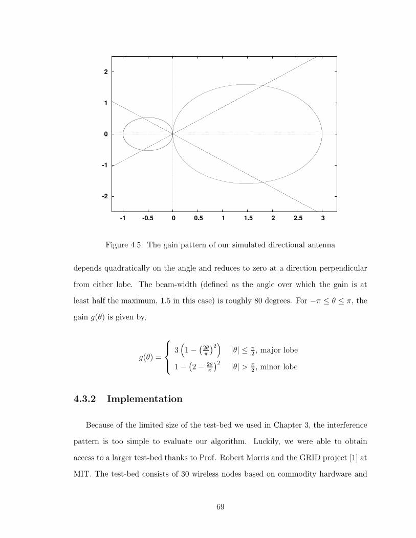
-2
-1
0
1
2
-1 -0.5 0 0.5 1 1.5 2 2.5 3
Figure 4.5. The gain pattern of our simulated directional antenna
depends quadratically on the angle and reduces to zero at a direction perpendicular
from either lobe. The beam-width (defined as the angle over which the gain is at
least half the maximum, 1.5 in this case) is roughly 80 degrees. For −π ≤ θ ≤ π, the
gain g(θ) is given by,
g(θ) =
3(
1−(
2θπ
)2)
|θ| ≤ π2, major lobe
1−(
2− 2θπ
)2|θ| > π
2, minor lobe
4.3.2 Implementation
Because of the limited size of the test-bed we used in Chapter 3, the interference
pattern is too simple to evaluate our algorithm. Luckily, we were able to obtain
access to a larger test-bed thanks to Prof. Robert Morris and the GRID project [1] at
MIT. The test-bed consists of 30 wireless nodes based on commodity hardware and
69
software placed on a single floor of an office building. The hardware consists of small
form-factor computers equipped with a 266 MHz Geode processor and 128MB of
RAM. Each computer is also equipped with a Netgear [5] tri-mode mini-PCI wireless
Ethernet adapter. This card is capable of operating in 802.11a,b and g modes, but
we conduct all our experiments in 802.11a mode to avoid interference with another
production 2.4GHz wireless network operating in same environment. The software
platform uses Linux and the Click modular router [38] and was very similar to our
previous test-bed; hence we were able to use our implementation of OML without
modifications. In addition, we implemented our interference detection algorithm also
on top of Click.
4.4 Results
We present the results from our evaluation in this Section. We first explain the
different metrics that we use in Section 4.4.1. Next, we show the results from our
simulations and our testbed in Sections 4.4.2 and 4.4.3 respectively.
4.4.1 Evaluation Metrics
In this Chapter, we are primarily interested in finding out how quickly and ac-
curately we are able to infer interference. We also compare our performance against
the 1-hop and 2-hop heuristics. We defer the discussion of performance of end-to-end
flows to Chapter 5. In particular, we try to answer the following questions here:
1. Are there any interfering pairs of active links that are not detected by our
algorithm? (False Negatives)
70

2. Do we erroneously infer interference between pairs of links that do not interfere
with each other? (False Positives)
3. How long do we allow interfering links to transmit at the same time before we
detect the interference?
4.4.2 Simulation
For our simulations, we create a wireless network by placing 30 nodes uniformly
at random in a rectangular region. The height of the rectangle is twice the radio
range and the width is changed to vary the density of node placement. We use static
pre-configured routes to avoid any undesirable interactions between the execution of
a routing protocol and our algorithm. Each data point is obtained by averaging over
8 simulation runs unless otherwise specified. We use α = 0.5 and β = 0.8 in all
our experiments; recall that once we infer interference between two links, OML will
prevent them from sending in the same time-slot, thus limiting each to roughly half
the throughput. We simulate 802.11b radios at 2Mbps in all cases.
4.4.2.1 Accuracy of Interference Inference
In this experiment, we first fix the average density of network at 16 nodes per radio
range (the area of the circle covered by the transmitter of each node). We then simu-
late ten simultaneous flows generated between randomly chosen (source,destination)
pairs while varying the signal propagation model at the physical layer. We then look
at interference between links that were on the paths of any one of these 10 flows.
Table 4.1 shows the false positives and negatives for various methods of determining
interference. The ‘1-hop’ and ‘2-hop’ methods refer to heuristics based on the network
distance between the senders of each link. In the case of our passive measurement
71
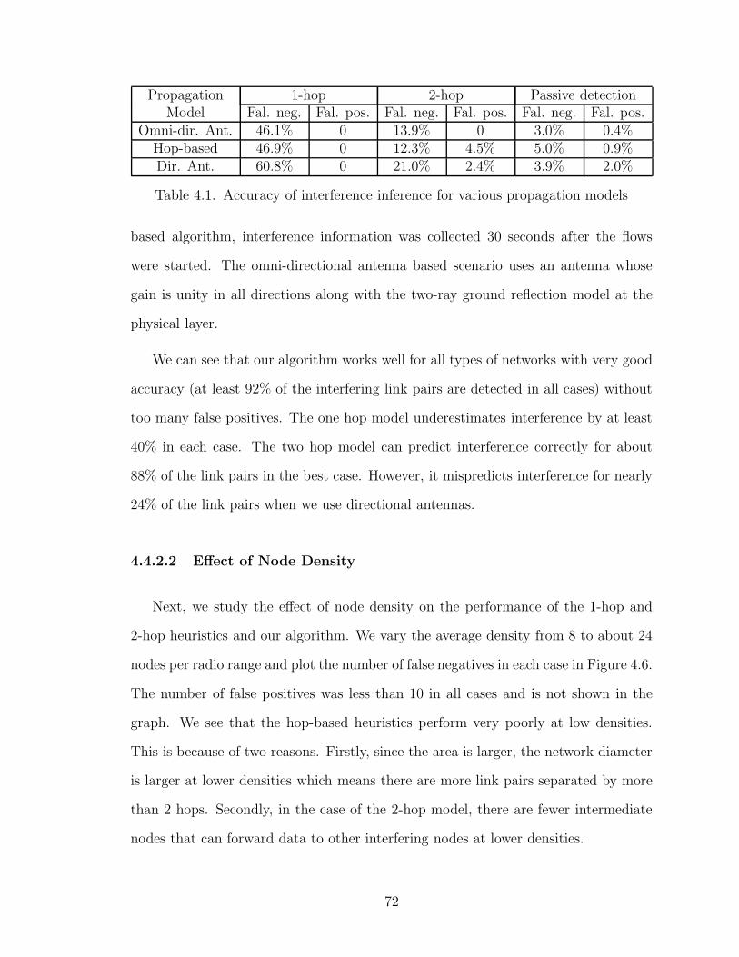
Propagation 1-hop 2-hop Passive detectionModel Fal. neg. Fal. pos. Fal. neg. Fal. pos. Fal. neg. Fal. pos.
Omni-dir. Ant. 46.1% 0 13.9% 0 3.0% 0.4%Hop-based 46.9% 0 12.3% 4.5% 5.0% 0.9%Dir. Ant. 60.8% 0 21.0% 2.4% 3.9% 2.0%
Table 4.1. Accuracy of interference inference for various propagation models
based algorithm, interference information was collected 30 seconds after the flows
were started. The omni-directional antenna based scenario uses an antenna whose
gain is unity in all directions along with the two-ray ground reflection model at the
physical layer.
We can see that our algorithm works well for all types of networks with very good
accuracy (at least 92% of the interfering link pairs are detected in all cases) without
too many false positives. The one hop model underestimates interference by at least
40% in each case. The two hop model can predict interference correctly for about
88% of the link pairs in the best case. However, it mispredicts interference for nearly
24% of the link pairs when we use directional antennas.
4.4.2.2 Effect of Node Density
Next, we study the effect of node density on the performance of the 1-hop and
2-hop heuristics and our algorithm. We vary the average density from 8 to about 24
nodes per radio range and plot the number of false negatives in each case in Figure 4.6.
The number of false positives was less than 10 in all cases and is not shown in the
graph. We see that the hop-based heuristics perform very poorly at low densities.
This is because of two reasons. Firstly, since the area is larger, the network diameter
is larger at lower densities which means there are more link pairs separated by more
than 2 hops. Secondly, in the case of the 2-hop model, there are fewer intermediate
nodes that can forward data to other interfering nodes at lower densities.
72
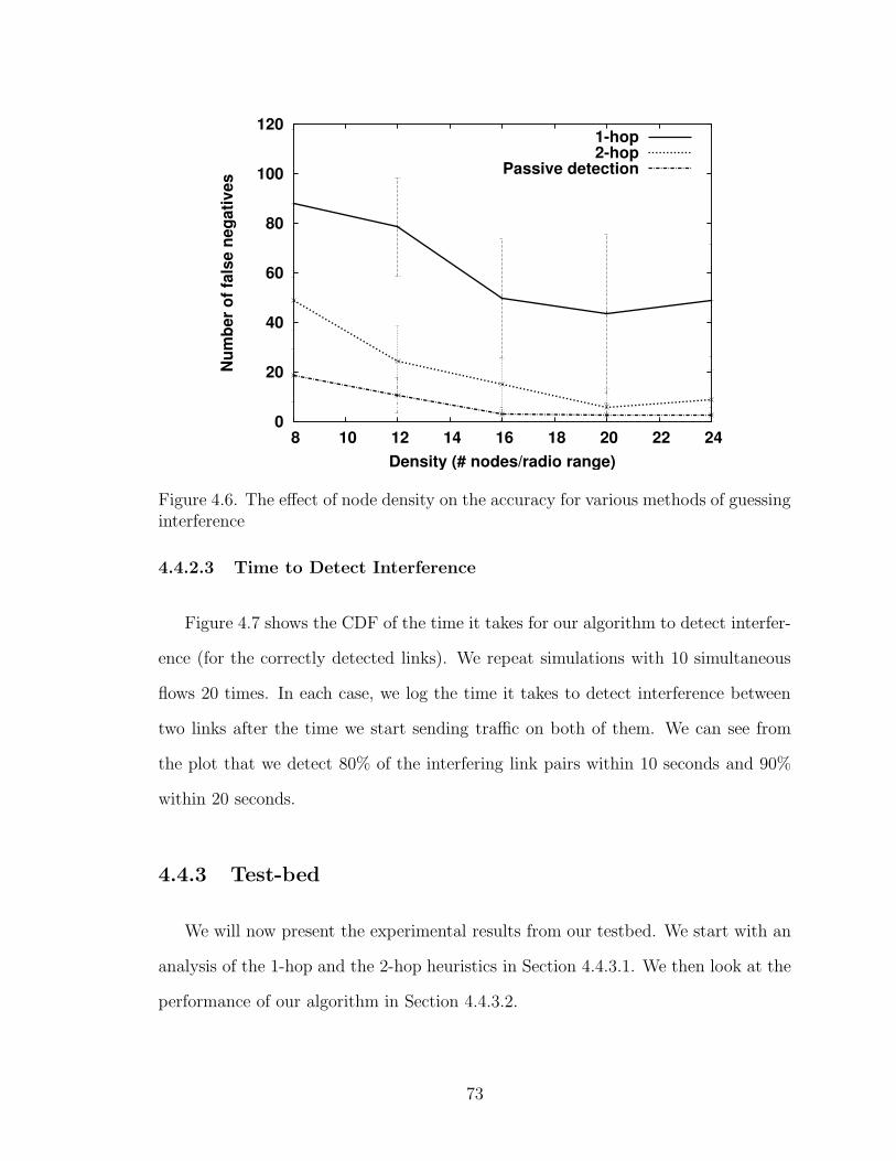
0
20
40
60
80
100
120
8 10 12 14 16 18 20 22 24
Num
ber o
f fal
se n
egat
ives
Density (# nodes/radio range)
1-hop2-hop
Passive detection
Figure 4.6. The effect of node density on the accuracy for various methods of guessinginterference
4.4.2.3 Time to Detect Interference
Figure 4.7 shows the CDF of the time it takes for our algorithm to detect interfer-
ence (for the correctly detected links). We repeat simulations with 10 simultaneous
flows 20 times. In each case, we log the time it takes to detect interference between
two links after the time we start sending traffic on both of them. We can see from
the plot that we detect 80% of the interfering link pairs within 10 seconds and 90%
within 20 seconds.
4.4.3 Test-bed
We will now present the experimental results from our testbed. We start with an
analysis of the 1-hop and the 2-hop heuristics in Section 4.4.3.1. We then look at the
performance of our algorithm in Section 4.4.3.2.
73

0
0.1
0.2
0.3
0.4
0.5
0.6
0.7
0.8
0.9
1
0 10 20 30 40 50 60
Perc
enta
ge o
f lin
ks
Time to detect interference (s)
Figure 4.7. The CDF of the time taken to detect interference
4.4.3.1 Performance of 1-hop and 2-hop heuristics
In our first experiment, we measured the loss rate for broadcast packets (mod-
ulated at 6 Mbps at the physical layer) sent from each node in our network. We
say that a link exists from node A to B if B can receive at least 75% of the packets
broadcast by A. According to this definition, there were 191 links in our network.3
Next, we measured the interference between all pairs of links by using the method-
ology described in [46]. By using broadcast packets, we only had to conduct(
30
2
)
= 435
experiments each lasting about 30 seconds. Of the 18,145 link pairs, there were 5125
pairs that did not interfere. In other words, there was a 72% chance that any given
pair of links would interfere.
Table 4.2 shows the performance of the 1-hop and the 2-hop heuristics for these
links. We can see that the 1-hop heuristic has few false positives whereas the 2-
3There were only 6 node pairs where the reception rate was between 20% and 80%. Therefore,any choice of the threshold in this range would’ve resulted in a similar number of links.
74
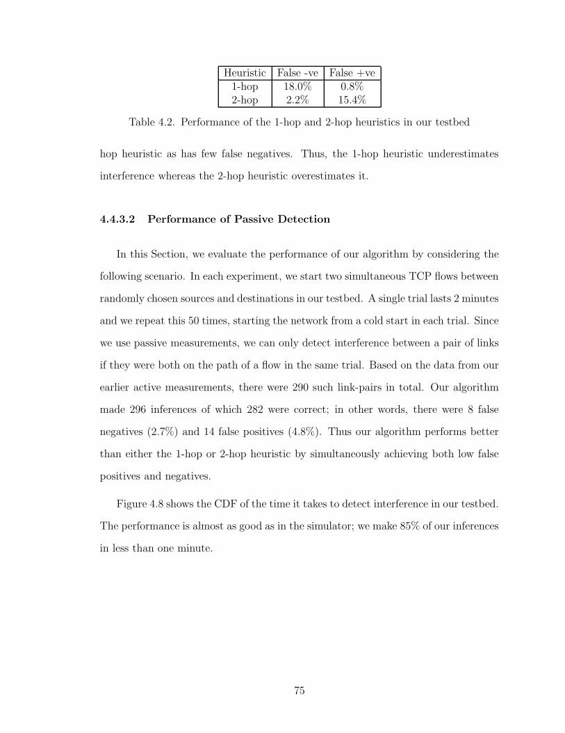
Heuristic False -ve False +ve1-hop 18.0% 0.8%2-hop 2.2% 15.4%
Table 4.2. Performance of the 1-hop and 2-hop heuristics in our testbed
hop heuristic as has few false negatives. Thus, the 1-hop heuristic underestimates
interference whereas the 2-hop heuristic overestimates it.
4.4.3.2 Performance of Passive Detection
In this Section, we evaluate the performance of our algorithm by considering the
following scenario. In each experiment, we start two simultaneous TCP flows between
randomly chosen sources and destinations in our testbed. A single trial lasts 2 minutes
and we repeat this 50 times, starting the network from a cold start in each trial. Since
we use passive measurements, we can only detect interference between a pair of links
if they were both on the path of a flow in the same trial. Based on the data from our
earlier active measurements, there were 290 such link-pairs in total. Our algorithm
made 296 inferences of which 282 were correct; in other words, there were 8 false
negatives (2.7%) and 14 false positives (4.8%). Thus our algorithm performs better
than either the 1-hop or 2-hop heuristic by simultaneously achieving both low false
positives and negatives.
Figure 4.8 shows the CDF of the time it takes to detect interference in our testbed.
The performance is almost as good as in the simulator; we make 85% of our inferences
in less than one minute.
75

0
0.1
0.2
0.3
0.4
0.5
0.6
0.7
0.8
0.9
1
0 20 40 60 80 100
Perc
enta
ge o
f lin
k pa
irs
Time to detect interference (s)
Figure 4.8. The CDF of the time taken to detect interference in our testbed
76
Chapter 5
End-to-end Fairness using Local
Weights
In the Chapter, we present End-to-end Fairness using Local Weights (EFLoW), a
distributed transport-layer algorithm that can compute the correct local weights to be
used at the MAC layer. EFLoW provides Max-Min fairness (as defined in Section 5.1)
between competing flows. We describe the design of EFLoW in detail in Section 5.2.
Finally, we present results from our simulations and experiments in Section 5.3.
5.1 Max-Min fairness
While there are many different definitions of fairness used in wireless network
literature [12], Max-Min fairness appears to be the most popular choice among re-
searchers [60, 61, 51, 41]. The key idea behind Max-Min fairness is that we should
not provide more throughput to any flow if it prevents us from giving at-least as much
throughput to other flows [12]. Weighted Max-Min fairness is a generalization of this
approach with support for weights, and is formally defined below.
77
5.1.1 Max-Min Fairness
Consider a network with n flows. Let fi be the throughput received by the i-th
flow. The allocation is said to be Max-Min fair if for each flow i, an allocation of
fi + ε1 is possible only by reducing the allocation of another flow j to fj − ε2 where
fj < fi. On the other hand, if we can find a subset H of flows {m1, m2, . . . , mk},
which all have throughput higher than fi, and if we can increase the throughput of
fi by only decreasing the throughput of flows from H, then the allocation is not fair.
Informally, Max-Min fairness states that inequality in throughput of flows is al-
lowed under the condition that penalizing the richer flows wouldn’t provide any ben-
efits to the poorer flows. On the other hand, if we can provide better service to any
flow by only penalizing flows that receive a higher throughput, then the allocation is
not Max-Min fair.
The above definition does not provide any means to differentiate service between
flows. A simple method to address this limitation is to associate a weight with
each flow. When comparing two flows, we always check if their throughputs are in
proportion to their weights. More formally, if flow fi is assigned a weight of wi, we
make a simple change to the above definition by modifying the condition that fj < fi
to fj/wj < fi/wi. Similarly, for all t : ft ∈ H, ft/wt > fi/wi.
To illustrate this definition, consider the example in Figure 5.1, which shows a
network with three flows (f1, f2, f3). Assume an interference model where two links
interfere if and only if they share an end-point. Then, (a), (b) and (c) are three
possible allocations in terms of the fraction of time for which the source is active. It
is easy to see that (a) is unfair because we can increase f1 without decreasing any other
flow’s allocation. Similarly, (b) is not fair because we can increase f3 by decreasing
f2 and f2 > f3. Finally, (c) is fair even though f1 receives twice the throughput of
78

A
B
DC E
f2
f3
f1
0.25f3
0.25f2
0.4f1
0.2f3
0.3f2
0.5f1
0.25f3
0.25f2
0.5f1
(a) (b) (c)
Figure 5.1. Example for Max-Min Fair allocation
the other flows. This is because node C is already saturated and we cannot increase
f2 or f3 even if we decrease f1.
Weighted Fair Queueing (WFQ) [21] is a popular method for providing Max-Min
fairness when all flows compete for the same resource. WFQ states that throughput
must be assigned to flows in proportion to their weight. If the allocation to any
flow is more than its demand, the surplus is again divided among the rest of the
flows in proportion of their weights. This process continues until there is either no
surplus capacity or when all demands are satisfied. In wired networks, per-hop WFQ
guarantees end-to-end Max-Min fairness. But because of the shared nature of the
medium, this is not true for wireless networks.
79

5.2 Achieving End-to-end Fairness
In this Section, we describe EFLoW , a distributed transport layer algorithm for
achieving end-to-end fairness. Though our current implementation of EFLoW uses
WSA, it can also work on top any MAC layer that provides the higher layers control
over resource allocation within a single contention neighborhood. More specifically,
we assume that the MAC layer allows the transport layer to dynamically associate a
weight with each node, and allocates transmission opportunities to each node in a con-
tention region proportional to its weight by implementing a Weighted Fair Queueing
(WFQ) discipline [21].
We use the term local weight to refer to the weights at the MAC layer. They
are only used to resolve conflicts between directly competing nodes. In contrast, the
weights defined in Section 5.1 are assigned to flows (not nodes or links) and have
global significance. In Section 5.2.1, we detail our system model, and show why
achieving end-to-end fairness is hard even when the MAC provides support for local
fairness. We then present the design of EFLoW in Section 5.2.2.
5.2.1 System Model
For ease of explanation, we first consider a network in which all nodes are in the
same contention region. We generalize this to a multi-hop network in the next step.
5.2.1.1 Stage 1: Single Contention Region
Consider a simple network consisting of three nodes (A, B and C), where there are
three flows originating at each node (Figure 5.2). Scheduling happens at two levels in
our system. First, within a node, we have to decide which packet will be sent to the
wireless interface. Second, at the MAC layer, we have to decide which node transmits
80

in each time slot. Unless otherwise specified, we assume that a node uses WFQ to
schedule its flows [21].
Since all nodes compete with each other, ideally we would like to achieve the
functionality of a single WFQ system with six queues. Thus, to achieve max-min
fairness, we have to assign to each node a local weight that is the sum of the weights
of all its backlogged flows. Note that a flow f is said to be backlogged at a node N if
the arrival rate of f at N is greater than its service rate. For instance, the weight of
node A, WA, should be computed as WA = w11 + w12 + w13, assuming that all flows
of node A are backlogged. In this case, the allocation to the first flow is given by,
f11 =w11
w11 + w12 + w13
× (Alloc. to A at MAC)
=w11
w11 + w12 + w13
×WA
WA + WB + WC× C
=w11
WA + WB + WC
× C
Thus, computing a schedule at the MAC layer requires knowledge of the demands
of all six flows as well as the capacity C at the MAC layer.
5.2.1.2 Stage 2: Mutli-hop Network
To illustrate the additional challenges that arise in a multi-hop network, we revisit
the example topology in Figure 5.1. For a multi-hop network, a contention region is
defined as a maximal set of nodes where all pairs interfere with each other. Since
no two nodes in the same region can transmit simultaneously, the total allocation in
each region has to be less than the channel capacity. Assuming a one-hop interference
model, Figure 5.3 shows a network in which (a) there are multiple contention regions
and (b) the same node (node C) is a part of multiple contention regions. The final
allocation to node C is the minimum of its allocation from regions 1 and 2. So if we
81
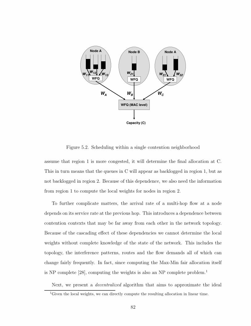
Node A
WFQw11
w12 w13
Node B
WFQ
w21
Node A
WFQw31 w32
WFQ (MAC level)
WA WB WC
Capacity (C)
Figure 5.2. Scheduling within a single contention neighborhood
assume that region 1 is more congested, it will determine the final allocation at C.
This in turn means that the queues in C will appear as backlogged in region 1, but as
not backlogged in region 2. Because of this dependence, we also need the information
from region 1 to compute the local weights for nodes in region 2.
To further complicate matters, the arrival rate of a multi-hop flow at a node
depends on its service rate at the previous hop. This introduces a dependence between
contention contexts that may be far away from each other in the network topology.
Because of the cascading effect of these dependencies we cannot determine the local
weights without complete knowledge of the state of the network. This includes the
topology, the interference patterns, routes and the flow demands all of which can
change fairly frequently. In fact, since computing the Max-Min fair allocation itself
is NP complete [28], computing the weights is also an NP complete problem.1
Next, we present a decentralized algorithm that aims to approximate the ideal
1Given the local weights, we can directly compute the resulting allocation in linear time.
82
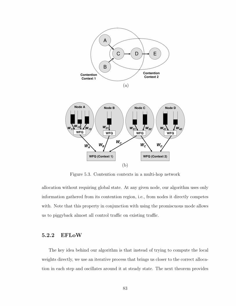
A
B
DC E
Contention Context 1
Contention Context 2
(a)
Node A
WFQw11
w12 w13
Node B
WFQ
w21
Node C
WFQw31 w32
WFQ (Context 1)
WAWB
WC
Node D
WFQw41 w42
WFQ (Context 2)
WC WD
(b)
Figure 5.3. Contention contexts in a multi-hop network
allocation without requiring global state. At any given node, our algorithm uses only
information gathered from its contention region, i.e., from nodes it directly competes
with. Note that this property in conjunction with using the promiscuous mode allows
us to piggyback almost all control traffic on existing traffic.
5.2.2 EFLoW
The key idea behind our algorithm is that instead of trying to compute the local
weights directly, we use an iterative process that brings us closer to the correct alloca-
tion in each step and oscillates around it at steady state. The next theorem provides
83
the theoretical building block of our design by providing an alternate characterization
of Max-Min fairness.
Definition 1. If flow f1 is backlogged at node N1, we define this backlog to be a
permissible backlog in a contention region C iff for every flow f2 passing through
node N2 ∈ C, the service rate of f2 at N2 is no greater than the service rate of f1 at
N1 (in proportion to the weights of f1 and f2).
Theorem 2. The allocation is Max-Min fair if and only if every node where any flow
is backlogged is a permissible in at least one contention region.
Proof. For ease of explanation, we assume that every flow has unit weight (the proof
can easily be generalized to non-unit weights). The proof is by contradiction.
=⇒: Assume the contrary, i.e., there is a flow f backlogged at a node N which is
impermissible in every contention region Cj that N is a part of. In other words, there
is at least one flow fj through Nj ∈ Cj where fj > f . By reducing the allocation
to all fj, there is some surplus capacity in every contention region that contains N .
Thus we can increase the allocation to N and hence to f , which violates the definition
in Section 5.1.
⇐=: We first make the observation that in order to increase the allocation f of a
flow, we have to increase its allocation at at-least one node N where it is backlogged.
In order to do this we have to decrease the transmit rate of at least one node Nj in
every contention region Cj such that N ∈ Cj. Without loss of generality, assume that
the backlog at N is permissible in C1. Since no flow at Nj ∈ C1 is being serviced
faster than f , we cannot decrease the allocation of Nj without violating the definition
of Max-Min fairness.
Note that the condition in Theorem 2 can be verified at each node using only in-
84

formation gathered from its own contention neighborhood(s). In contrast, our earlier
definition required a global view of the network. In a nutshell, our approach is to
identify impermissible backlogs and use an additive-increase multiplicative-decrease
algorithm (similar to the TCP’s congestion control algorithm) to adapt the weights
to fix it. Initially, we set the local weights of all nodes to 1 and perform the following
operations periodically:
1. Service nodes using their current local weights for a time window, W . W is a
system-wide constant expressed in terms of the number of time slots. Within
each window, each node receives a number of time slots proportional to its
weight.
2. Estimate the service rate of a unit-weight backlogged flow at each node over
the previous window.
3. Compare each backlogged node N ’s service rate with the service rate of ev-
ery node it competes with. If there are nodes with a higher service in every
contention region N is a part of, add N to the set I.
4. At the beginning of each time window, add a positive constant α to the local
weight of all nodes in the set I (additive increase). Reduce the local weight of
all other nodes by multiplying it by (1− β) where β is a constant between zero
and one (multiplicative decrease).
Note that step 3 identifies all nodes with impermissible backlogs and adds them
to the set I. In step 4, we increase the weights of all these nodes while decreasing
the weight of nodes which are either (a) not backlogged or (b) have only permissible
backlogs. This moves to system closer to its ideal state in the next time window.
To implement step 2, each node has to keep track of the service rates of its queues.
Since we use a virtual time (VT) based implementation of WFQ for scheduling flows
85
within a node, the required book-keeping is already taken care of. Recall that VT
measures the service (i.e., the number of bits) received by a continuously backlogged
flow with unit-weight. Let tW be the start of a window period, and let N.VT(t) denote
the virtual time of node N at time t. Then, N.VT(tW +W )−N.VT(tW ) represents the
service received by a continuously backlogged flow during the window starting at tW .
Note that this service is exactly the value we need at step 2 within a multiplicative
constant, i.e., 1/W . Thus, at step 3 we can directly use the progress of the virtual
time in the previous window to compare the service rate of queues at different nodes.
Step 4 requires broadcasting the the service rates of queues in a two-hop neigh-
borhood. For 1-hop neighbors, this is easily accomplished by including the current
virtual-time as part of the EFLoW header of every packet. By listening in promiscu-
ous mode, nodes can easily determine the service rates of their immediate neighbors.
In order to disseminate this information to 2-hop neighbors, every node also includes
a list of its 1-hop neighbors and their service rates in the EFLoW header.2 As in
Chapter 4, 3-hop neighbors which interfere are treated as a special case - we explic-
itly request a 1-hop neighbor to forward information about them. Due to this lazy
approach, nodes may not always have the most up-to-date information about their
two-hop neighbors. But in practice, we found that the AIMD algorithm is robust
enough to converge despite this limitation.
Figure 5.4 shows the pseudocode for updating the local weights. We experimented
with values of W = 20 and W = 40 time slots and found that either choice works
well in practice. The function queue.ExpWtAvg() returns the exponentially weighted
average queue size which we use to determine if the node is backlogged.
2The EFLoW header is variable in length, and was 48 bytes on average in our experiments.Further optimizations (compression, differential coding etc.) are possible, but are outside the scopeof this work.
86

function Node::ProcessEndWindow()
//first check if we are backlogged
if queue.ExpWtAvg() < congestionThreshold
//not congested hence multiplicative decrease
weight ← weight × (1− β)
return
myServiceRate ← VT(currTime) −
VT(currTime − W)
minMaxServiceRate ← ∞
for all C ∈ N.GetContentionRegions()
cServiceRate = C.GetMaxServiceRate()
if cServiceRate < minMaxServiceRate
minMaxServiceRate = cServiceRate
endfor
if minMaxServiceRate > myServiceRate
//additive increase
weight ← weight + α
else
//congested, but must go into MD
weight ← weight × (1− β)
Figure 5.4. Pseudocode for the function executed by every node at the end of W timeslots
87

5.3 Results
We have implemented EFLoW on top of OML in both ns-2 and in Click. We
present results from our simulations in Section 5.3.1 followed by the results from the
MIT test-bed in Section 5.3.2. But first, we start with a brief overview of the metrics
we use.
The two important aspects of the system we wish to quantify are its efficiency and
fairness. To quantify the fairness of the outcome, we again use the fairness index as
defined in Section 3.4. One possible way to quantify efficiency is to simply look at the
average throughput of a flow in the system. However, a key drawback of this metric is
that the resource demands for supporting a given throughput is not the same across
different flows. For example, it takes three times as many wireless transmissions to
provide the same throughput to a flow routed over three hops compared to a flow
where the source and sink can communicate directly. Instead, we use the number of
useful transmissions per second as the metric for efficiency. A packet transmission is
considered to be useful if (a) the packet is eventually delivered to the end point of
the flow and (b) the packet is not a duplicate when it is received at the end point.
If we overestimate the interference pattern, OML and EFLoW will prevent links
from sending at the same time even though they do not interfere. This means that our
efficiency will suffer compared to using the correct interference pattern. On the other
hand, if we underestimate interference, links that do interfere with each other will
be allowed to transmit in the same time slot. As a result, the accuracy of resource
allocation in OML will suffer, and hence the fairness seen by EFLoW will also be
suboptimal.
88

5.3.1 Simulations
We have implemented our algorithm in ns2 for the following three reasons. Firstly,
we can easily change the topology or the size of the network in a simulator. Secondly,
the simulator allows us to implement an Oracle which uses global state to approximate
the ideal allocation. We use this Oracle (see Section 5.3.1.2) for comparison with
EFLoW. Thirdly, the simulator allows us to implement an idealized TDMA MAC so
that we can evaluate EFLoW independent of the inefficiencies introduced by OML
(see Section 5.3.1.1).
As in Chapter 4, we simulate 802.11b radios at 2Mbps in each of our experiments.
RTS/CTS was disabled in all the experiments because there is no need for it when
using time slots. Surprisingly we saw better fairness and throughput with RTS/CTS
disabled even when not using OML or a TDMA MAC. As reported in some earlier
work [22, 7], our observations confirm that the overhead of RTS/CTS is not justified
in relation to the number of collisions it prevents.
5.3.1.1 TDMA MAC Protocol
Since OML is designed to run on 802.11 hardware without any changes to the
standard, it has a number of limitations compared to a TDMA MAC implemented
with hardware support. For example, OML uses time-slots which are long enough to
send 10 packets of about 1500 bytes each. The clock synchronization and enforce-
ment at the boundaries of slots are not perfect either. In order to evaluate EFLoW
independent of these limitations, we have implemented an idealized TDMA MAC in
ns-2 as follows. The slot duration is calculated as the time it takes to transmit an
MTU-sized packet, receive an acknowledgment plus a guard time3 of 200 microsec-
3The guard time is a short idle time between two slots. It is used in TDMA MACs to providerobustness against clock drift and small errors in clock synchronization.
89

onds. We decided to implement link-layer acknowledgments to prevent unnecessary
retransmissions and time-outs at the TCP layer. We included carrier-sensing also
to protect against imperfect interference information while using the 1-hop or 2-hop
heuristics.
5.3.1.2 Ideal Allocation
As mentioned earlier, computing the ideal allocation is a hard problem even in
the case of a simulation. Instead of trying to compute it exactly, we use the following
slot allocation algorithm (called the Oracle) to approximate the ideal schedule. The
algorithm uses global knowledge to sort all nodes based on how much service their
queues are receiving. We can then prioritize assignment of slots to nodes which have
received less service. The pseudocode for the Oracle is shown in Figure 5.5. Note
that this is only an approximation since we break ties arbitrarily in GetLeastServiced.
To quantify the benefits of EFLoW, our first step is to look at the convergence
time of our iterative algorithm (Section 5.3.1.3). Next, we look at the effect of the
number of simultaneous flows in Section 5.3.1.4. After that, we study the impact of
the accuracy of the interference pattern in Section 5.3.1.6 followed by the effect of the
traffic pattern in Section 5.3.1.5. Finally, we study the performance of TCP flows in
Section 5.3.1.7 and the scaling behavior of EFLoW when increasing the network size
in Section 5.3.1.8.
5.3.1.3 Convergence of EFLoW
To get a better understanding of the convergence of EFLoW, we start by looking
at the effect of the parameters α and β. In order to do this, we first construct a
network of 30 nodes with an average density of 16 nodes per radio range. Nodes
are equipped with omni-directional antennas and the signal propagation follows the
90
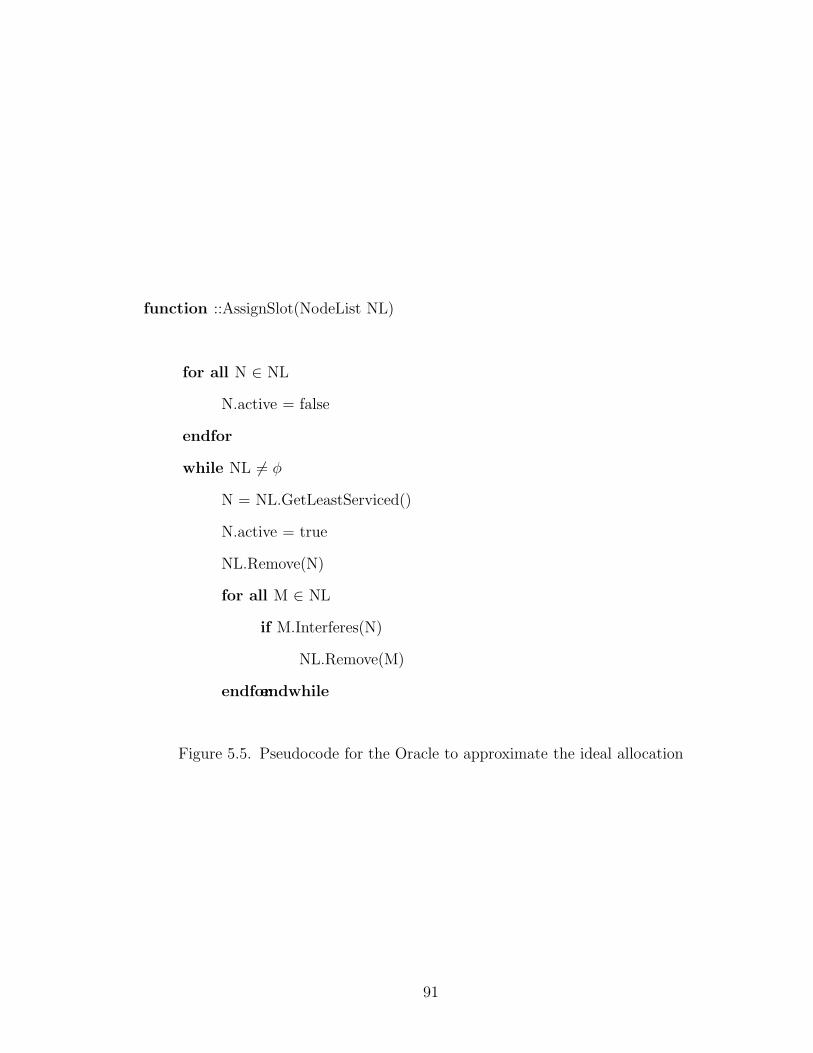
function ::AssignSlot(NodeList NL)
for all N ∈ NL
N.active = false
endfor
while NL 6= φ
N = NL.GetLeastServiced()
N.active = true
NL.Remove(N)
for all M ∈ NL
if M.Interferes(N)
NL.Remove(M)
endforendwhile
Figure 5.5. Pseudocode for the Oracle to approximate the ideal allocation
91

two-ray ground reflection model. We simulate 8 simultaneous flows with a duration
of 30 seconds in each experiment. We also record the throughput of each flow at the
end of 2 seconds and 5 seconds. The traffic pattern is a star i.e., sources are chosen
at random but all flows terminate at the same node.4
Figure 5.6 shows the fairness index as a function of α (β is fixed at 0.5). Since we
are only trying to look at the convergence process, we simulate the TDMA protocol
described in Section 5.3.1.1. We also assume that the exact interference pattern is
available for the MAC layer; this can easily be obtained from global state in the
simulator. Surprisingly, the fairness index (especially after 30 seconds) does not vary
much even when we change α by nearly three orders of magnitude (from 0.001 to
0.5). This reason for this follows from the fact that the absolute values of the local
weights do not matter in WSA; the allocation would be the same even if we multiply
all local weights by the same constant factor. Therefore, the behavior of EFLoW will
also not change if we multiply both α and the initial weights by the same constant.
In other words, multiplying α by a constant c has the same effect as dividing the
initial weights by c. Thus, Figure 5.6 shows that the value of α does not affect the
convergence of EFLoW; the differences in fairness at 5 seconds (due to differences in
the initial conditions) disappear after 30 seconds.
Next, we fix α = 0.5 and vary β from 0.001 to 0.9 and plot the fairness in
Figure 5.7. We can see that the value of β has a much greater effect on the fairness.
As mentioned in [16], higher values of β lead to both quicker convergence and larger
oscillations after convergence. β = 0.5 appears to be the best compromise; the fairness
after 5s is comparable to using higher values of β. At the same time the oscillations
are small also; the standard deviation in fairness after 30 seconds is the lowest for
β = 0.5.
4We consider the star traffic pattern to be indicative of the scenario where all nodes are tryingto reach the same wired gateway.
92

0.6
0.65
0.7
0.75
0.8
0.85
0.9
0.95
1
0.001 0.01 0.1 1
Fairn
ess
Inde
x
alpha (beta fixed at 0.5)
2 second flows5 second flows
30 second flows
Figure 5.6. Effect of the additive increase parameter α on fairness.
0.6
0.65
0.7
0.75
0.8
0.85
0.9
0.95
1
0.001 0.01 0.1 1
Fairn
ess
Inde
x
beta (alpha fixed at 0.5)
2 second flows5 second flows
30 second flows
Figure 5.7. Effect of the multiplicative decrease parameter β on fairness.
93

0
0.2
0.4
0.6
0.8
1
5 10 15 20 25 30
Fairn
ess
Inde
x
Duration of the flows (s)
802.11OML w/ static weight
TDMA w/ static weightOML w/ EFLoW
TDMA w/ EFLoW
Figure 5.8. Effect of the duration of the flows on fairness with and without EFLoW
Finally, we compare the performance of EFLoW with that of (a) the standard
802.11 protocol and (b) WSA with static weights, i.e., we do not use EFLoW, by
plotting the fairness as a function of the duration of the flows in Figure 5.8. We
repeat (a) and (b) for both OML and the TDMA MAC. We can see that both OML
and the TDMA MAC do not perform well with static weights; the fairness index,
while better than 802.11, is below 0.7 in all cases. This shows that fairness within a
single contention neighborhood does not directly give us end-to-end fairness in multi-
hop wireless networks. EFLoW converges within 10 seconds irrespective of the length
of the slots; the fairness index is better than 0.9 in both cases.
5.3.1.4 Effect of the number of flows
In this experiment, we construct the network as in the previous section and sim-
ulate between 2 and 10 simultaneous flows each lasting 100 seconds. Figures 5.9
and 5.10 plot the fairness index for OML and the TDMA MAC respectively. The
94

0
0.2
0.4
0.6
0.8
1
1.2
2 3 4 5 6 7 8 9 10
Fairn
ess
Inde
x
Number of Simultaneous Flows
802.11WSA w/ static weight
EFLoWOracle
Figure 5.9. Effect of the number of simultaneous flows on fairness with and withoutEFLoW when using the TDMA MAC (star traffic)
802.11 MAC shows poor fairness (index below 0.6) when there are 6 or more flows.
OML with static weights does not improve on this much. On the other hand, EFLoW
shows very little degradation in fairness even with a large number of flows; the fair-
ness index is always greater than 0.9 (0.95 with the TDMA MAC). The Oracle yields
a fairness index which is almost exactly 1 in all cases.
Next, we compare the utilization of the transmission medium under various
schemes. WSA and EFLoW can lead to some inefficiency due to the control overheads.
However, the efficiency can also suffer under 802.11 because of the poor fairness; a lot
of transmissions may not reach their destination if an intermediate hop experiences
starvation. To quantify this overhead, we plot the number of useful transmissions
per second versus the number of flows in Figures 5.11 and 5.12 (for the TDMA MAC
and OML respectively). The efficiency of EFLoW is close to, and in most cases even
better than 802.11.
95

0
0.2
0.4
0.6
0.8
1
1.2
2 3 4 5 6 7 8 9 10
Fairn
ess
Inde
x
Number of Simultaneous Flows
802.11OML w/ static weight
EFLoWOracle
Figure 5.10. Effect of the number of simultaneous flows on fairness with and withoutEFLoW when using OML (star traffic)
0
50
100
150
200
250
2 3 4 5 6 7 8 9 10
Usef
ul tr
ansm
issi
ons
per s
econ
d
Number of Simultaneous Flows
802.11WSA w/ static weights
EFLoWOracle
Figure 5.11. Effect of the number of simultaneous flows on utilization with andwithout EFLoW when using the TDMA MAC (star traffic)
96
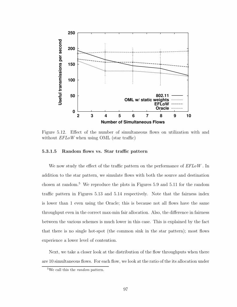
0
50
100
150
200
250
2 3 4 5 6 7 8 9 10
Usef
ul tr
ansm
issi
ons
per s
econ
d
Number of Simultaneous Flows
802.11OML w/ static weights
EFLoWOracle
Figure 5.12. Effect of the number of simultaneous flows on utilization with andwithout EFLoW when using OML (star traffic)
5.3.1.5 Random flows vs. Star traffic pattern
We now study the effect of the traffic pattern on the performance of EFLoW . In
addition to the star pattern, we simulate flows with both the source and destination
chosen at random.5 We reproduce the plots in Figures 5.9 and 5.11 for the random
traffic pattern in Figures 5.13 and 5.14 respectively. Note that the fairness index
is lower than 1 even using the Oracle; this is because not all flows have the same
throughput even in the correct max-min fair allocation. Also, the difference in fairness
between the various schemes is much lower in this case. This is explained by the fact
that there is no single hot-spot (the common sink in the star pattern); most flows
experience a lower level of contention.
Next, we take a closer look at the distribution of the flow throughputs when there
are 10 simultaneous flows. For each flow, we look at the ratio of the its allocation under
5We call this the random pattern.
97
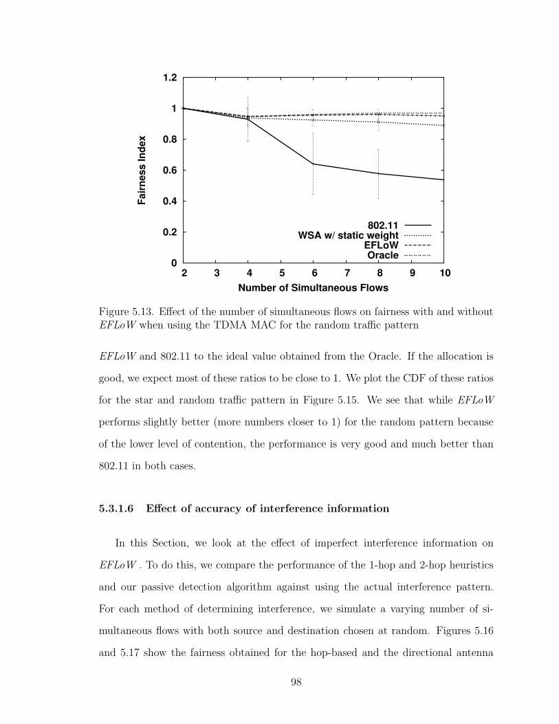
0
0.2
0.4
0.6
0.8
1
1.2
2 3 4 5 6 7 8 9 10
Fairn
ess
Inde
x
Number of Simultaneous Flows
802.11WSA w/ static weight
EFLoWOracle
Figure 5.13. Effect of the number of simultaneous flows on fairness with and withoutEFLoW when using the TDMA MAC for the random traffic pattern
EFLoW and 802.11 to the ideal value obtained from the Oracle. If the allocation is
good, we expect most of these ratios to be close to 1. We plot the CDF of these ratios
for the star and random traffic pattern in Figure 5.15. We see that while EFLoW
performs slightly better (more numbers closer to 1) for the random pattern because
of the lower level of contention, the performance is very good and much better than
802.11 in both cases.
5.3.1.6 Effect of accuracy of interference information
In this Section, we look at the effect of imperfect interference information on
EFLoW . To do this, we compare the performance of the 1-hop and 2-hop heuristics
and our passive detection algorithm against using the actual interference pattern.
For each method of determining interference, we simulate a varying number of si-
multaneous flows with both source and destination chosen at random. Figures 5.16
and 5.17 show the fairness obtained for the hop-based and the directional antenna
98
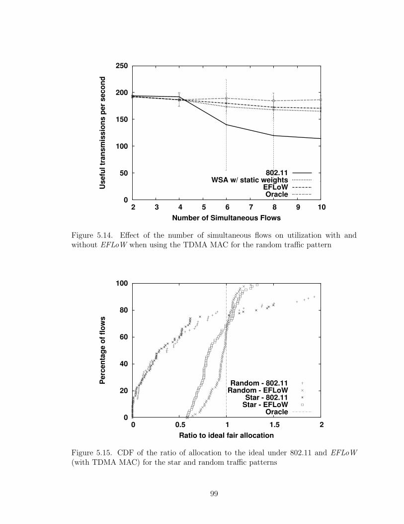
0
50
100
150
200
250
2 3 4 5 6 7 8 9 10
Usef
ul tr
ansm
issi
ons
per s
econ
d
Number of Simultaneous Flows
802.11WSA w/ static weights
EFLoWOracle
Figure 5.14. Effect of the number of simultaneous flows on utilization with andwithout EFLoW when using the TDMA MAC for the random traffic pattern
0
20
40
60
80
100
0 0.5 1 1.5 2
Perc
enta
ge o
f flo
ws
Ratio to ideal fair allocation
Random - 802.11Random - EFLoW
Star - 802.11Star - EFLoW
Oracle
Figure 5.15. CDF of the ratio of allocation to the ideal under 802.11 and EFLoW(with TDMA MAC) for the star and random traffic patterns
99

0
0.2
0.4
0.6
0.8
1
2 3 4 5 6 7 8 9 10
Fairn
ess
Inde
x
Number of Simultaneous Flows
802.111-hop2-hop
Passive detectionActual interference
Figure 5.16. The effect of the interference information on fairness when usingEFLoW(Hop-based interference)
based propagation models respectively (see Section 4.3 for more information about
these models). We can see that though the reduced accuracy of the 1-hop and 2-hop
heuristics affects the fairness of EFLoW, especially in the case of directional anten-
nas, we still obtain better performance than 802.11 in all cases. On the other hand,
the performance when using our detection algorithm is almost as good as having the
exact interference pattern.
Figure 5.18 looks at the efficiency obtained for the hop-based interference model.
We can see that the few false positives that we get with our learning algorithm do not
impact system efficiency by much. However, the 2-hop model leads to about 18% loss
of efficiency even though the number of false positives is very similar. This is explained
by the fact that the amount of information available for detecting interference is
directly proportional to the amount of traffic carried by a link. Thus our algorithm
tends to have better accuracy for the more important links. We obtained similar
results for the directional antenna based propagation model also (see Figure 5.19).
100

0
0.2
0.4
0.6
0.8
1
2 3 4 5 6 7 8 9 10
Fairn
ess
Inde
x
Number of Simultaneous Flows
802.111-hop2-hop
Passive detectionActual interference
Figure 5.17. The effect of the interference information on fairness when usingEFLoW(Directional antenna)
0
50
100
150
200
250
2 3 4 5 6 7 8 9 10
Num
ber o
f Use
ful T
rans
mis
sion
s/s
Number of Simultaneous Flows
802.111-hop2-hop
Passive detectionActual interference
Figure 5.18. The effect of the interference information on efficiency when usingEFLoW(Hop-based interference)
101
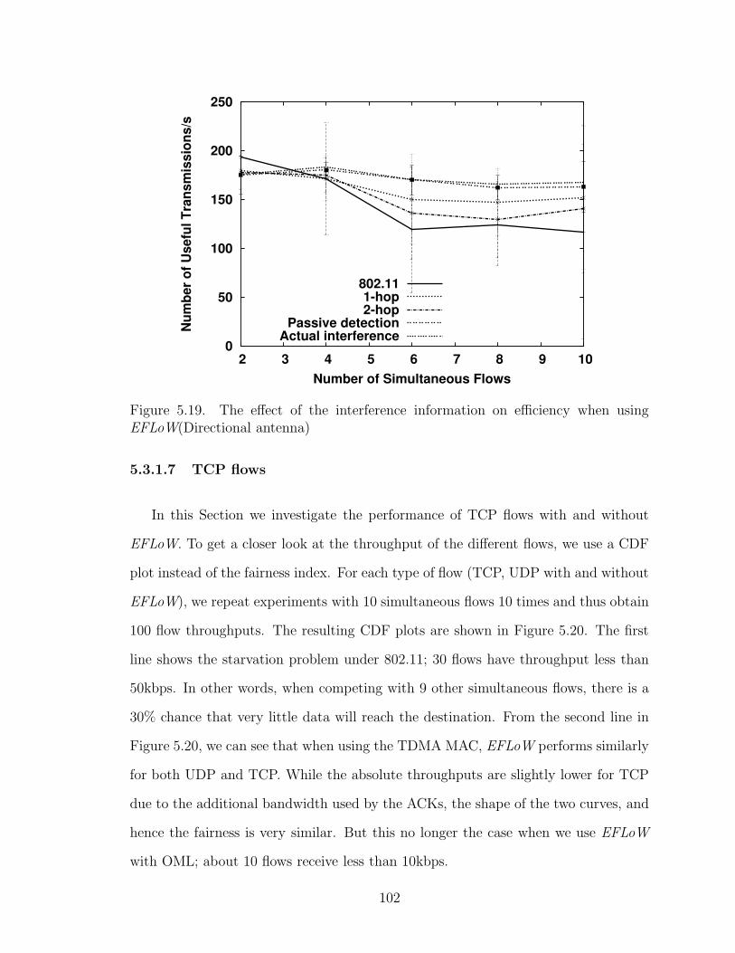
0
50
100
150
200
250
2 3 4 5 6 7 8 9 10
Num
ber o
f Use
ful T
rans
mis
sion
s/s
Number of Simultaneous Flows
802.111-hop2-hop
Passive detectionActual interference
Figure 5.19. The effect of the interference information on efficiency when usingEFLoW(Directional antenna)
5.3.1.7 TCP flows
In this Section we investigate the performance of TCP flows with and without
EFLoW. To get a closer look at the throughput of the different flows, we use a CDF
plot instead of the fairness index. For each type of flow (TCP, UDP with and without
EFLoW), we repeat experiments with 10 simultaneous flows 10 times and thus obtain
100 flow throughputs. The resulting CDF plots are shown in Figure 5.20. The first
line shows the starvation problem under 802.11; 30 flows have throughput less than
50kbps. In other words, when competing with 9 other simultaneous flows, there is a
30% chance that very little data will reach the destination. From the second line in
Figure 5.20, we can see that when using the TDMA MAC, EFLoW performs similarly
for both UDP and TCP. While the absolute throughputs are slightly lower for TCP
due to the additional bandwidth used by the ACKs, the shape of the two curves, and
hence the fairness is very similar. But this no longer the case when we use EFLoW
with OML; about 10 flows receive less than 10kbps.
102
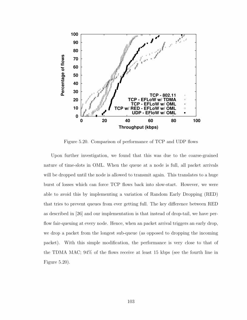
0
10
20
30
40
50
60
70
80
90
100
0 20 40 60 80 100
Perc
enta
ge o
f flo
ws
Throughput (kbps)
TCP - 802.11TCP - EFLoW w/ TDMA
TCP - EFLoW w/ OMLTCP w/ RED - EFLoW w/ OML
UDP - EFloW w/ OML
Figure 5.20. Comparison of performance of TCP and UDP flows
Upon further investigation, we found that this was due to the coarse-grained
nature of time-slots in OML. When the queue at a node is full, all packet arrivals
will be dropped until the node is allowed to transmit again. This translates to a huge
burst of losses which can force TCP flows back into slow-start. However, we were
able to avoid this by implementing a variation of Random Early Dropping (RED)
that tries to prevent queues from ever getting full. The key difference between RED
as described in [26] and our implementation is that instead of drop-tail, we have per-
flow fair-queuing at every node. Hence, when an packet arrival triggers an early drop,
we drop a packet from the longest sub-queue (as opposed to dropping the incoming
packet). With this simple modification, the performance is very close to that of
the TDMA MAC; 94% of the flows receive at least 15 kbps (see the fourth line in
Figure 5.20).
103

0
0.2
0.4
0.6
0.8
1
1.2
20 25 30 35 40 45 50
Fairn
ess
Inde
x
Number of Nodes
802.11EFLoW
Figure 5.21. Effect of the network size on the performance of 802.11 and EFLoW(with OML)
5.3.1.8 Scaling Network Size
In this experiment, we simulate 5 simultaneous flows while scaling the network
size from 20 to 50 nodes. In each case, the nodes are distributed at random in a
square area; the dimensions of the square are varied to keep the average node density
constant at 25 per radio range. The average fairness index for each case is shown in
Figure 5.21. We can see that the performance of 802.11 progressively worsens as we
increase the network size, whereas EFLoW shows only a slight degradation.
5.3.2 Test-bed
We now present the results from experiments on the MIT test-bed described in
Section 4.3.2. Once again, we use static routing based on measurement of link quality
in advance. We look at the performance of long-lived TCP flows in Sections 5.3.2.1
and 5.3.2.2 followed by the performance of short flows in Section 5.3.2.3.
104

802.11 1-hop 2-hop Passive Actualdetection interference
Averagesystem throughput 1.618 1.485 1.382 1.387 1.418
(Mbps)Average no.
of useful 273.5 268.2 257.0 261.2 268.0transmissions (/s)
Table 5.1. Efficiency of various schemes for 2 simultaneous flows in the test-bed.
5.3.2.1 Two simultaneous flows
In this experiment, we study the performance of two simultaneous TCP flows in
our test-bed. We pick two random sources and sinks and measure the throughput
of both flows over 2 minutes. We determine the interference pattern by either using
heuristics, our passive detection algorithm or the actual measured interference pattern
obtained in Section 4.4.3.1.
We repeat the experiment 50 times, and in each case measure F both with default
802.11 as well as with EFLoW and plot the CDF of F in Figure 5.22. Recall that
since there are two flows, F takes values from 0.5 (least fair) to 1 (most fair). We see
that without EFLoW, one of the two flows is starved (F ≈ 0.5) in 38% of the cases;
this never happens when using EFLoW with the correct interference pattern. We see
good fairness with the 2-hop heuristic because it has very few false negatives in our
test-bed (as mentioned earlier, false positives do not affect the fairness of EFLoW ).
The passive detection algorithm performs almost identically.
Table 5.1 shows the efficiency of our system in each case. The system throughput
is defined as the sum of the throughput of both flows in each trial. However, as
mentioned earlier, this metric is biased towards schemes that give higher priority to
flows routed over fewer network hops (such as 802.11). The difference between the
various schemes is much lower when we look at the number of useful transmissions. We
105

0
0.1
0.2
0.3
0.4
0.5
0.6
0.7
0.8
0.9
1
0.5 0.6 0.7 0.8 0.9 1
Perc
enta
ge o
f exp
erim
ents
Fairness Index
802.111-hop2-hop
Passive detectionActual interference
Figure 5.22. The CDF of the fairness index of two simultaneous TCP flows in thetest-bed
expect the efficiency of the 2-hop heuristic to be lower due to the large number of false
positives, but in practice, the difference is very small especially when compared to the
passive detection algorithm. This is because of two reasons. First, the efficiency of the
2-hop heuristic is only affected when it overestimates interference for the bottleneck
link of a flow, which is usually the link experiencing the most interference. Because
of the high level of interference in our test-bed (recall that 72% of the link pairs
interfere), the bottleneck is likely to interfere with almost all the other links and
hence very unlikely to be affected by false positives. Second, the advantage of our
passive detection algorithm is further diminished because of the delay in detecting
interference. Therefore, we don’t see as much improvement as when using the actual
interference pattern.
Based on these results, one could argue that the 2-hop heuristic is sufficient for
our test-bed. However, this depends on a number of factors that may not always be
true. Other applications may be more sensitive to false positives than EFLoW. There
106

0
0.1
0.2
0.3
0.4
0.5
0.6
0.7
0.8
0.9
1
0.3 0.4 0.5 0.6 0.7 0.8 0.9 1
Perc
enta
ge o
f exp
erim
ents
Fairness Index
802.111-hop2-hop
Passive detectionActual interference
Figure 5.23. The CDF of the fairness index of three simultaneous TCP flows in thetest-bed
may be more links pairs that do not interfere if the nodes are spread over a larger
area. As shown in our simulations, the type of antennas is a crucial factor as well.
The key advantage of passive measurements is that the algorithm can automatically
correct for all these factors without any modifications.
5.3.2.2 Three simultaneous flows
In this Section, we conduct 50 experiments as before, with the change that there
are three simultaneous flows in each experiment. The CDF of the resulting through-
puts is shown in Figure 5.23. Note that F = 0.333 if two of the 3 flows are starved,
which happens in roughly 25% of the cases under 802.11. If one of the flows is starved,
F lies between 0.33 and 0.66 depending on the distribution between the other two
flows. Finally F > 0.66 implies that all three flows were able to establish a connec-
tion; this happens in 80% of the cases when we use the actual interference pattern.
107
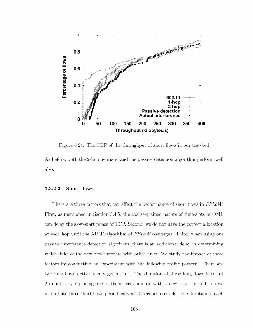
0
0.2
0.4
0.6
0.8
1
0 50 100 150 200 250 300 350 400
Perc
enta
ge o
f flo
ws
Throughput (kilobytes/s)
802.111-hop2-hop
Passive detectionActual interference
Figure 5.24. The CDF of the throughput of short flows in our test-bed
As before, both the 2-hop heuristic and the passive detection algorithm perform well
also.
5.3.2.3 Short flows
There are three factors that can affect the performance of short flows in EFLoW.
First, as mentioned in Section 3.4.5, the coarse-grained nature of time-slots in OML
can delay the slow-start phase of TCP. Second, we do not have the correct allocation
at each hop until the AIMD algorithm of EFLoW converges. Third, when using our
passive interference detection algorithm, there is an additional delay in determining
which links of the new flow interfere with other links. We study the impact of these
factors by conducting an experiment with the following traffic pattern. There are
two long flows active at any given time. The duration of these long flows is set at
2 minutes by replacing one of them every minute with a new flow. In addition we
instantiate three short flows periodically at 15 second intervals. The duration of each
108

of these flows is chosen at random between 2 to 10 seconds. Thus there are 2 long
flows and up to 3 short flows active at any given time.6 We run this experiment for
15 minutes and plot the CDF of the throughput of the short flows in Figure 5.24.
A throughput of zero indicates that a TCP connection was not established during
the duration of the flow. We can see that this happens for almost 44% of the flows
when we use the standard 802.11 MAC. However, with EFLoW, all the short flows
were able to establish a connection when using the actual interference pattern. The
performance is not as good while using the 2-hop heuristic or our passive detection
algorithm, but is still much better than the 802.11 MAC protocol.
6The short flows model web browsing and the long flows model file sharing applications anddownloads.
109

Chapter 6
Conclusions
Recently, there has been a lot of excitement about multi-hop wireless networks
built using commodity hardware. Deployments have become wide spread thanks
to the inexpensive and ready availability of 802.11 based hardware. However, the
observed performance have been disappointing especially while trying to support
multiple users at the same time. In this work, we have proposed a set of solutions that
can alleviate this problem by giving all nodes fair and efficient access to the wireless
medium. Though our primary target is mesh networks, we believe our approach is
also applicable to other scenarios such as sensor and vehicular networks.
The first component of our solution is the Overlay MAC Layer. OML implements
a time-slot based scheduler on top of any other MAC protocol. This allows us to
experiment with existing 802.11 based hardware. The ability to modify the MAC
without changes to standards is not only important to save costs but also to save
time; standards take a very long time to emerge since they have to satisfy the needs
and demands of a lot of different entities and applications. Also, since OML is based
on time slots, it avoids various problems that have plagued contention-based MACs
in multi-hop networks. Ultimately, the overlay approach will enable us to experiment
110
with new scheduling and bandwidth management algorithms, and evaluate their ben-
efits to existing applications, before implementing them in hardware at the MAC
layer; WSA and EFLoW are only a first step in this direction.
In order to reap the benefits of OML we need an accurate picture of which links
interfere with each other. We found previously used heuristics to be inadequate and
active measurements are expensive in terms of both resources and time. Motivated by
the fact that OML (and many other applications) only need interference information
for links that are in use, we develop an algorithm based on passive measurements
as an alternative. Our approach measures interference for exactly the links we need
without introducing any additional traffic in the network. We have demonstrated the
power of this approach by comparing it with other heuristics and show that it can
quickly and accurately determine the interference pattern for a wide variety of traffic
patterns and network scenarios.
Even with a method to control allocation within a local neighborhood (OML),
achieving end-to-end fairness in multi-hop networks is not an easy problem. Most
previous work assumes that state about the entire network can be consolidated at
a single node, which can lead to a very high control overhead. The distributed
approaches either assume a restricted traffic patterns or are tied to a particular con-
tention based MAC. Our solution, EFLoW, addresses the above mentioned limitations
by using an additive-increase multiplicative-decrease (AIMD) based algorithm. By
using EFLoW and WSA, we are able to both compute a fair allocation and a time-slot
based schedule to achieve that allocation, without the need for a centralized coordi-
nator. In addition, our approach does not restrict the traffic pattern in any way and
automatically adapts to changes in flow demands and network topology.
111

6.1 Open Issues and Future Work
We now mention some open issues and discuss possible avenues for future research.
Before we delve into specific components like OML or EFLoW, we first look at the
system as a whole.
System-wide issues: So far, all of our experiments (including simulations)
have been done with fixed nodes. While we have included some basic mechanisms
to handle mobility in all our algorithms, we have not evaluated them yet. Mobility
will definitely degrade the performance of our system, but to what extent is yet to be
determined. Further modifications might be necessary, especially when the mobility
is very high as in some sensor and vehicular networks.
WSA works well only when all nodes sharing the channel implement it. If there
are other nodes using the standard 802.11 protocol, the aggregate bandwidth of all
nodes using WSA will be limited to that of one node using 802.11. To address
this limitation, both EFLoW and WSA have to be modified to make nodes more
aggressive in trying to transmit data. The additional traffic will affect the accuracy
of our interference detection algorithm also; more sophisticated mechanisms based on
machine learning or other statistical techniques might help in factoring out the effect
of external senders.
Overlay MAC Layer: The current slot length (time to transmit 10 packets) used
by OML might be too long for certain real-time applications. TCP performance can
also be improved by using more fine grained scheduling. We believe that more can
be done to optimize this aspect of OML. First, we must analyze the implementation,
identify bottlenecks, and mitigate them when possible; interrupt priority and using
call-backs versus polling are two areas that can be improved. Secondly, modifications
to the firmware of the Network Interface Card (NIC) could provide additional benefits.
Finally, packet fragmentation might be necessary to achieve better enforcement at the
112

boundaries of time-slots. Currently, we simply transmit the whole packet even if we
are close to the end of a slot and do not have enough time to transmit without spilling
over to the next slot.
Interference Detection: While our approach based on passive measurements is
indeed very promising, we have assumed that the link qualities and the interference
pattern are stable enough to be tracked; more measurements are needed to confirm
the types of networks where this true. Also, our algorithm currently works on top
of time-slot based MACs only; it may be possible to generalize this to contention
based MACs by monitoring the queue lengths, back-off windows and the number of
collisions. Another avenue that is worth exploring is whether passive measurements
can be combined with the modeling based approaches used in [55] and [49]. This
might help improve the detection time and to move beyond a pair-wise interference
model. Lastly, we have only used our interference measurements for one application -
scheduling with OML. We plan to study other applications such as channel assignment
and admission control in the future. Also, the routing protocol may also be able to
exploit availability of interference information by picking paths that don’t interfere
with each other; however, this requires information about links that are not (yet)
carrying any traffic. It would be interesting to see how we can satisfy this requirement
by augmenting passive measurements with periodic probing of new paths and other
active measurements.
End-to-end fairness: Though we have empirically shown that EFLoW can provide
max-min fairness for a number of scenarios, a formal proof of convergence remains
an open problem. Also, we have not investigated whether EFLoW can be adapted to
other definitions of fairness; examples include proportional fairness, allocations which
try to maximize a utility function and so on.
Though both TCP and EFLoW use AIMD based algorithms, the mechanisms that
113

change the local weights and the window size proceed independently of each other.
This may be suboptimal because EFLoW might decrease the allocation while TCP is
increasing the window size and vice versa. We plan to see whether performance can
be improved by synchronizing the two processes; for example by dropping a packet
every time EFLoW does a multiplicative decrease.
EFLoW does not provide any delay guarantees; we have only looked at the
throughput of flows so far. We plan to look at how we can augment EFLoW to
support real-time traffic; one possible method is to reserve certain time-slots for
specific flows in advance. Lastly, more experiments are needed to understand the
performance of EFLoW with more realistic workloads. Replaying actual traffic logs
or using application level benchmark suites will be very useful in this regard.
114
Bibliography
[1] MIT Grid Project, http://www.pods.lcs.mit.edu/grid/.
[2] MadWifi, http://madwifi.sourceforge.net/.
[3] Meraki Networks, http://www.meraki.com/.
[4] Mesh Networks LLC, http://www.meshnetworksllc.com/.
[5] Netgear, http://www.netgear.com/.
[6] the network simulator - ns2, http://www.isi.edu/nsnam/ns/.
[7] MIT Roofnet, http://www.pdos.lcs.mit.edu/roofnet/.
[8] Andersen, D., H. Balakrishnan, F. Kaashoek, and R. Morris, Resilient OverlayNetworks, in SOSP, 2001.
[9] Banerjee, S., B. Bhattacharjee, and C. Kommareddy, Scalable application layermulticast, in SIGCOMM, 2002.
[10] Bao, L., and J. J. Garcia-Luna-Aceves, Distributed Dynamic Channel AccessScheduling for Ad Hoc Networks, in Journal of Parallel and Distributed Com-puting, 2002.
[11] Bao, L., and J. J. Garcia-Luna-Aceves, Hybrid Channel Access Scheduling in AdHoc Networks., in ICNP, 2002.
[12] Bertsekas, D., and R. Gallagher, Data Networks, Prentice Hall, 1987.
[13] Bhagwat, P., B. Raman, and D. Sanghi, Turning 802.11 Inside-Out, in HotNets-II, 2003.
[14] Bharghavan, V., S. Lu, and T. Nandagopal, Fair Queueing in Wireless Networks:Issues and Approaches, IEEE Personal Communications Magazine, 1999.
[15] Chen, S., and Z. Zhang, Localized algorithm for aggregate fairness in wirelesssensor networks, in MOBICOM, 2006.
[16] Chiu, D.-M., and R. Jain, Analysis of the increase and decrease algorithms forcongestion avoidance in computer networks, Comput. Netw. ISDN Syst., 17 (1),1989.
115

[17] Chlamtac, I., and S. Kutten, A spatial-reuse TDMA/FDMA for mobile multi-hop radio networks, in INFOCOM, 1987.
[18] Chu, Y.-H., S. G. Rao, and H. Zhang, A case for end system multicast, inSIGMETRICS, pp. 1–12, Santa Clara, CA, 2000.
[19] Cidon, I., and M. Sidi, Distributed Assignment Algorithms for Multihop PacketRadio Networks, IEEE Trans. Comput., 38 (10), 1353–1361, doi:http://dx.doi.org/10.1109/12.35830, 1989.
[20] Community Wireless Rooftop Systems, Wireless Networking reference - Com-munity Wiress/Rooftop Systems.
[21] Demers, A., S. Keshav, and S. Shenker, Analysis and simulation of a fair queueingalgorithm, in SIGCOMM, 1989.
[22] Draves, R., J. Padhye, and B. Zill, Comparison of Routing Metrics for Multi-HopWireless Networks, in SIGCOMM, 2004.
[23] Dugar, P., N. Vaidya, and P. Bahl, Priority and fair-scheduling over a wirelessLAN, in MILCOM, 2001.
[24] Ee, C. T., and R. Bajcsy, Congestion control and fairness for many-to-one routingin sensor networks, in SenSys ’04, pp. 148–161, ACM Press, New York, NY, USA,doi:http://doi.acm.org/10.1145/1031495.1031513, 2004.
[25] Elson, J., and D. Estrin, Time Synchronization for Wireless Sensor Networks,in PDPS Workshop on Parallel and Distributed Computing Issues in WirelessNetworks and Mobile Computing, pp. 186–186.
[26] Floyd, S., and V. Jacobson, Random early detection gateways for congestionavoidance, IEEE/ACM Transactions on Networking, 1 (4), 397–413, 1993.
[27] Fraleigh, C., S. Moon, B. Lyles, C. Cotton, M. Khan, D. Moll, R. Rockell,T. Seely, and S. C. Diot, Packet-level traffic measurements from the Sprint IPbackbone, IEEE Networks, 17 (6), 2003.
[28] Gambiroza, V., B. Sadeghi, and E. Knightly, End-to-End Performance and Fair-ness in Multihop Wireless Backhaul Networks, in MOBICOM, 2004.
[29] Garetto, M., T. Salonidis, and E. Knightly, Modeling Per-flow Throughput AndCapturing Starvation in CSMA Multi-hop Wireless Networks, in INFOCOM,2006.
[30] Gummadi, R., D. Wetherall, B. Greenstein, and S. Seshan, Understanding andmitigating the impact of RF interference on 802.11 networks, in SIGCOMM,2007.
[31] Heusse, M., F. Rousseau, G. Berger-Sabbatel, and A. Duda, Performanceanomaly of 802.11b, in INFOCOM, San Francisco, USA, 2003.
116

[32] Hohlt, B., L. Doherty, and E. Brewer, Flexible Power Scheduling for SensorNetworks, in IPSN, 2004.
[33] Jain, K., J. Padhye, V. Padmanabhan, and L. Qiu, Impact of Interference onMulti-hop Wireless Network Performance, in MOBICOM, 2003.
[34] Jain, K., J. Padhye, V. N. Padmanabhan, and L. Qiu, Impact of interference onmulti-hop wireless network performance, in MOBICOM, 2003.
[35] Jaiswal, S., G. Iannaccone, C. Diot, J. Kurose, and D. Towsley, Inferring TCPconnection characteristics through passive measurements, in INFOCOM, 2004.
[36] Johnson, D. B., D. A. Maltz, and J. Broch, DSR: The Dynamic Source RoutingProtocol for Multihop Wireless Ad Hoc Networks, in Ad Hoc Networking, 2001.
[37] Karhima, T., A. Silvennoinen, M. Hall, and S.-G. Haggman, IEEE 802.11b/gWLAN tolerance to jamming., in MILCOM, 2004.
[38] Kohler, E., R. Morris, B. Chen, J. Jannotti, and M. F. Kaashoek, The ClickModular Router, ACM Transactions on Computer Systems, 18 (3), 2000.
[39] Lee, W. Y., Mobile communications engineering, McGraw Hill, 1982.
[40] Lilley, J., J. Yang, H. Balakrishnan, and S. Seshan, A unified header compressionframework for low-bandwidth links, in MOBICOM, 2000.
[41] Luo, H., S. Lu, and V. Bharghavan, A new model for packet scheduling in mul-tihop wireless networks, in MOBICOM, 2000.
[42] Luo, L., M. Gruteser, H. Liu, D. Raychaudhuri, K. Huang, and S. Chen, A QoSrouting and admission control scheme for 802.11 ad hoc networks, in DIWANS,2006.
[43] Mitzenmacher, M., Compressed bloom filters, IEEE/ACM Trans. Netw., 10 (5),2002.
[44] Moffat, A., and J. Zobel, Parameterised compression for sparse bitmaps, in SI-GIR, 1992.
[45] of the IEEE Computer Society, L. M. S. C., Wireless LAN medium access control(MAC) and physical layer (PHY) specifications, IEEE Standard 802.11, 1999.
[46] Padhye, J., S. Agarwal, V. N. Padmanabhan, L. Qiu, A. Rao, and B. Zill, Esti-mation of link interference in static multi-hop wireless networks, in IMC, 2005.
[47] Parekh, A. K., and R. G. Gallager, A generalized processor sharing approach toflow control in integrated services networks: the single-node case, IEEE/ACMTrans. Netw., 1 (3), 344–357, doi:http://doi.acm.org/10.1145/159907.159914,1993.
117
[48] Perkins, C., Ad Hoc On Demand Distance Vector (AODV) Routing, IETF In-ternet Draft, 1997.
[49] Qiu, L., Y. Zhang, F. Wang, M. K. Han, and R. Mahajan, A general model ofwireless interference, in MOBICOM, 2007.
[50] Raman, B., and K. Chebrolu, Revisiting MAC Design for an 802.11-based MeshNetwork, in HOTNETS, 2004.
[51] Rangwala, S., R. Gummadi, R. Govindan, and K. Psounis, Interference-awarefair rate control in wireless sensor networks, SIGCOMM Comput. Commun. Rev.,36 (4), 2006.
[52] Raniwala, A., and T.-C. Chiueh, Architecture and algorithms for an IEEE802.11-based multi-channel wireless mesh network, in INFOCOM, 2005.
[53] Rao, A., and I. Stoica, An Overlay MAC Layer for 802.11 Networks, in MO-BISYS, 2005.
[54] Rappaport, T., Wireless Communications: Principles and Practice, PrenticeHall, 2001.
[55] Reis, C., R. Mahajan, M. Rodrig, D. Wetherall, and J. Zahorjan, Measurement-based models of delivery and interference in static wireless networks, SIGCOMMComput. Commun. Rev., 2006.
[56] Romer, K., Time synchronization in ad hoc networks, in Proceedings of the 2ndACM international symposium on Mobile ad hoc networking & computing, pp.173–182, ACM Press, 2001.
[57] Sadeghi, B., V. Kanodia, A. Sabharwal, and E. Knightly, Opportunistic mediaaccess for multirate ad hoc networks, in MOBICOM, 2002.
[58] Schmid, U., and K. Schossmaier, Interval-based Clock Synchronization, Real-Time Systems, 12 (2), 173–228, 1997.
[59] Silvester, J., Perfect scheduling in multi-hop broadcast networks, in ICCC, 1982.
[60] Sridharan, A., and B. Krishnamachari, Max-Min Fair Collision-Free Schedulingfor Wireless Sensor Networks, in IPCCC (Workshop on Mobile Wireless Net-works), 2004.
[61] Sridharan, A., and B. Krishnamachari, Maximizing network utilization withmax-min fairness in wireless sensor networks, ACM/Kluwer Wireless Networks,2008.
[62] Stoica, I., D. Adkins, S. Zhuang, S. Shenker, and S. Surana, Internet indirectioninfrastructure, in SIGCOMM, 2002.
118

[63] Sun, Y., E. M. Belding-Royer, X. Gao, and J. Kempf, Real-time traffic supportin heterogeneous mobile networks, Wirel. Netw., 13 (4), 2007.
[64] Taylor, D. E., A. Herkersdorf, A. Doring, and G. Dittmann, Robust headercompression (ROHC) in next-generation network processors, IEEE/ACM Trans.Netw., 13 (4), 2005.
[65] Waldspurger, C. A., and W. E. Weihl, Lottery Scheduling: Flexible Proportional-Share Resource Management, in Operating Systems Design and Implementation,pp. 1–11, 1994.
[66] Yi, Y., and S. Shakkottai, Hop-by-hop congestion control over a wireless multi-hop network, in Proc. of IEEE INFOCOM, 2004.
119


