

NBER WORKING PAPER SERIES
REALLOCATION, FIRM TURNOVER, ANDEFFICIENCY: SELECTION ON PRODUCTIVITY
OR PROFITABILITY?
Lucia FosterJohn Haltiwanger
Chad Syverson
Working Paper 11555http://www.nber.org/papers/w11555
NATIONAL BUREAU OF ECONOMIC RESEARCH1050 Massachusetts Avenue
Cambridge, MA 02138August 2005
We thank Susanto Basu, Steve Davis, Kevin Murphy, Mark Roberts, and Jim Tybout for helpful comments. We have also benefitted from seminar participants at Chicago, Duke, LSE, Minneapolis Fed, Purdue, Yale,NBER Summer Institute, Upjohn Conference, CAED, NBER Productivity Meetings, and the ASSAMeetings. The views expressed herein are those of the author(s) and do not necessarily reflect the views ofthe National Bureau of Economic Research.
©2005 by Lucia Foster, John Haltiwanger and Chad Syverson. All rights reserved. Short sections of text,not to exceed two paragraphs, may be quoted without explicit permission provided that full credit,including © notice, is given to the source.
Reallocation, Firm Turnover, and Efficiency: Selection on Productivity or Profitability?Lucia Foster, John Haltiwanger and Chad SyversonNBER Working Paper No. 11555August 2005JEL No. E2, L1, L6, O4
ABSTRACT
There is considerable evidence that producer-level churning contributes substantially to aggregate(industry) productivity growth, as more productive businesses displace less productive ones.However, this research has been limited by the fact that producer-level prices are typicallyunobserved; thus within-industry price differences are embodied in productivity measures. If pricesreflect idiosyncratic demand or market power shifts, high "productivity" businesses may not beparticularly efficient, and the literature's findings might be better interpreted as evidence of enteringbusinesses displacing less profitable, but not necessarily less productive, exiting businesses. In thispaper, we investigate the nature of selection and productivity growth using data from industrieswhere we observe producer-level quantities and prices separately. We show there are importantdifferences between revenue and physical productivity. A key dissimilarity is that physicalproductivity is inversely correlated with plant-level prices while revenue productivity is positivelycorrelated with prices. This implies that previous work linking (revenue-based) productivity tosurvival has confounded the separate and opposing effects of technical efficiency and demand onsurvival, understating the true impacts of both. We further show that young producers charge lowerprices than incumbents, and as such the literature understates the productivity advantage of newproducers and the contribution of entry to aggregate productivity growth.
Lucia FosterCenter for Economic StudiesBureau of the CensusRoom 211/WPIIWashington, DC [email protected]
John C. HaltiwangerDepartment of EconomicsUniversity of MarylandCollege Park, MD 20742and [email protected]
Chad SyversonDepartment of EconomicsUniversity of Chicago1126 East 59th StreetChicago, IL 60637and [email protected]

1. Introduction A robust finding of the large and growing literature using business-level microdata is that
within-industry reallocation and its associated firm turnover shape changes in industry
aggregates. The effect of this churning process on aggregate productivity has received particular
theoretical and empirical attention.
Models of such selection mechanisms characterize industries as collections of
heterogeneous-productivity producers and link producers’ productivity levels to their
performance and survival in the industry (see, for example, Jovanovic (1982), Hopenhayn
(1992), Ericson and Pakes (1995), and Melitz (2003)). The important mechanism driving
aggregate productivity movements in these models is the reallocation of market shares to more
efficient producers, either through market share shifts among incumbents or through entry and
exit. Low productivity plants are less likely to survive and thrive than their more efficient
counterparts, creating selection-driven aggregate (industry) productivity increases. Hence the
theories point to the productivity-survival link as a crucial driver of productivity growth.
The related empirical literature has documented this mechanism as a robust feature of
industry dynamics.1 Businesses’ measured productivity levels are persistent and vary
significantly within industries, suggesting that productivity “types” among producers have an
inherent idiosyncratic element. Reallocation, entry, and exit rates are large. Businesses with
higher measured productivity levels tend to grow faster and are more likely to survive than their
less productive industry cohorts. These signs all point to a selection mechanism being at work.
In reality, however, the productivity-survival link is a simplification. Selection is on
profitability, not productivity (though the two are likely correlated). Productivity is only one of
several possible idiosyncratic factors that determine profits, however. Other idiosyncratic factors
may affect survival as well.2
Given the empirical findings discussed above on the importance of productivity to
survival, does this theoretical simplification matter? There is reason to believe it may. A
limitation of empirical research with business microdata is that establishment-level prices are
typically unobserved. Previous studies have had to measure establishment output as revenue 1 Bartelsman and Doms (2000) review much of this literature. 2 While the models cited above and their literature counterparts do actually construct their selection mechanism on profits, productivity is the only idiosyncratic producer characteristic. Thus producer profits are a positive monotonic function of productivity, and selection on profits is equivalent to selection on productivity.
1

divided by a common industry-level deflator.3 Therefore within-industry price differences are
embodied in output and productivity measures. If prices reflect idiosyncratic demand shifts or
market power variation rather than quality or production efficiency differences, a reasonable
supposition for many industries, then high “productivity” businesses may not be particularly
technologically efficient.4 If this is the case, the empirical literature documents the importance
of selection on profits, but not necessarily productivity. Therefore the connection between
productivity and survival probability, reallocation, and industry dynamics may be overstated, and
the impact of demand-side influences on survival understated.
In this paper, we attempt to measure the separate influences of idiosyncratic productivity
and demand on selection. We can explore this bifurcation systematically because, unlike most of
the previous empirical work on the subject, we are able to observe both producers’ physical
outputs and prices. We can then directly measure physical efficiency (the quantity of physical
units of output produced per unit of input) as well as estimate idiosyncratic demand shocks at the
business level. We use these measures to look at the independent contributions of technology
and demand heterogeneity on producer dynamics and within-industry reallocation.
Our empirical strategy is to focus on establishments that produce homogeneous products.
This offers the advantage of minimizing across-producer quality differences, making it easier to
interpret our empirical results and match them to theory. Physical output measures are more
meaningful when quality variation is small. For example, one might reasonably consider two
plants’ outputs of 1000 cubic feet of ready-mixed concrete as equal outputs. This would be
much harder to do for, say, two automobile assemblers producing 1000 cars each. Focusing on
homogeneous products allows us to be more confident that our physical-output-based
productivity measure reflects producers’ true outputs, and that price variations indicate
differences in demand levels instead of quality differences. (Although below we further consider
in light of the evidence whether the price variation patterns we observe are consistent with this
3 Syverson (2004), which uses physical output data as we do in this study, is an exception to this. In addition, in a series of papers using Colombian data, Eslava et al. (2004, 2005a, 2005b) use plant-level output and input price data in a manner similar to that used here. The focus of the latter papers is in the impact of market reform on firm dynamics, but at the core the findings for Colombia are consistent with the findings reported here. 4 Input price variation is another possible business-specific profitability influence that could also show up in productivity measures. Businesses enjoying idiosyncratically low input prices will look as though they are hiring fewer inputs per unit output. While we abstract from the effects of input price variation here, Katayama, Lu, and Tybout (2003) and Gorodnichenko (2005) argue factor prices are potentially important. We see this area as a possible expansion point for future work.
2

supposedly small quality variation.) The specific products that we investigate are corrugated and
solid fiber boxes (henceforth referred to as boxes), white pan bread (bread), carbon black,
roasted coffee beans (coffee), ready-mixed concrete (concrete), oak flooring (flooring), motor
gasoline (gasoline), block ice, processed ice, hardwood plywood (plywood), and raw cane sugar
(sugar). Producers of these products make outputs that are among the most physically
homogeneous in the manufacturing sector. In addition to product homogeneity, the set of
producers is large enough to exhibit sufficiently rich within-industry reallocation and turnover.5
We are not the first to note the possible difficulties involved in using revenue-based
output and productivity measures when using microdata. Abbott (1992) documents the extent of
price dispersion within broad industries and outlines possible implications for measurement of
aggregates. Klette and Griliches (1996) and Mairesse and Jaumandreu (2005) consider how
intra-industry price fluctuations can affect production function and productivity estimates.
Melitz (2000), De Loecker (2005) and Gorodnichenko (2005) have extended these analyses to
accommodate multi-product producers and factor price variation. Katayama, Lu, and Tybout
(2003), whose theme perhaps most closely matches that of this paper, demonstrate that both
revenue-based output and expenditure-based input measures can lead to productivity
mismeasurement and incorrect interpretations about how heterogeneous producers respond to
shocks and the associated welfare implications. Each of these papers forwards an alternative
method of empirical inference that attempts to avoid the difficulties inherent in productivity
analysis when business-level price data is unavailable.
This paper shares an obvious common thread with this earlier work. It departs in that,
rather than trying to infer “true” technical efficiency using alternative estimation strategies, we
have the unusual opportunity to compute it with the data at hand. We can therefore directly
compare revenue-based productivity measures with measures of physical efficiency, and show
precisely the impacts of each on selection dynamics and industry evolution. We can further use
our business-level price observations to estimate the influence of idiosyncratic demand elements
on survival. We do not mean to imply that having to econometrically infer true technological
5 Seven of our products are in the group of thirteen products that Roberts and Supina (1996, 2000) use in their studies of establishment-level price variation. We could not use all thirteen products due to data availability issues. The four products that we study that are not used in the Roberts and Supina studies are carbon black, block ice, processed ice, and raw cane sugar. There are also a number of homogeneous-output industries with large numbers of businesses outside of the manufacturing sector. Unfortunately, the microdata for these other sectors lacks the detailed production information necessary for this study.
3

productivity is a weakness of the earlier research. Indeed, the thrust of those papers was to seek
alternate inference methods, given that revenue-based output measures are so ubiquitous. We
instead seek to take advantage of observing both “standard” microdata and the much more rare
quantity data in order to determine definitively (at least for our sample industries) the differences
between revenue-based and physical output measures. The hope is, of course, that our findings
for a small subset of industries offer insight into these links in the broader economy.
To preview our findings, we find that the large and persistent within-industry dispersion
observed in revenue-based productivity measures is also present in prices and physical-quantity-
based productivity measures. Interestingly, physical productivity is actually more dispersed than
revenue-based productivity even though the former is a component of the latter. This pattern
reflects the fact that, while the two productivity measures are highly correlated with each other,
physical productivity is negatively correlated with establishment-level prices while revenue
productivity is positively correlated with prices. The negative physical productivity-price
correlation is consistent with equilibria where producers are price setters and more efficient
businesses find it optimal to pass along their cost savings through lower prices.
We exploit the observed variation in prices, physical output and physical productivity to
estimate plants’ idiosyncratic demand levels. Our physical productivity measures provide a
unique and powerful instrument for price that allows us to overcome the typical simultaneity bias
in demand estimation. The demand estimates permit us to decompose plant-level price variation
into two components, one reflecting movements along the demand curve due to differences in
physical efficiency, and the other reflecting producers’ idiosyncratic demand shock.
With regard to industry evolution, we find that exiting businesses have lower productivity
levels—either revenue based or physical quantity based—than incumbents, though the gap is
larger in magnitude for revenue productivity. Entering businesses, on the other hand, have
higher physical productivity levels than incumbents, but their revenue-based productivity
advantage is much less pronounced and sometimes nonexistent. Similar patterns are seen when
we compare young businesses to their more mature competitors. For all of these findings, the
key source of discrepancies between the estimated effects of revenue and physical productivity is
that young businesses charge lower prices than incumbents. This also suggests that the current
literature understates the contribution of entry to aggregate productivity growth.
4

We bring these pieces together to explore the determinants of market selection. As in the
existing literature, we find that plants with lower revenue productivity are more likely to exit.
When we decompose revenue productivity into physical productivity and prices, though, we find
that both independently affect survival and the magnitudes of their individual effects are larger
than their combined effect through revenue productivity measures. That is, while low prices and
low physical productivity are both associated with higher probabilities of exit in isolation, the
marginal effect of each is substantially enhanced by controlling for the other. When we further
decompose prices into technology and demand fundamentals, our analysis shows that producers
facing lower demand shocks are more likely to exit. In fact, our estimates suggest that demand
variations across producers are the quantitatively dominant factor in determining survival.
The paper proceeds as follows. The next section provides the theoretical motivation for
the paper by highlighting the multi-dimensional nature of selection with a simple model of
imperfect competition among producers that differ not only in their cost/productivity levels, but
also in the idiosyncratic demand conditions they face. Section 3 describes the data and
measurement issues involved in our empirical study. Basic empirical facts about productivity
and price distributions in our industries are then discussed in Section 4, and the central results
regarding selection dynamics are presented in Section 5. Section 6 concludes.
2. Theoretical Motivation We now construct a model that shows how idiosyncratic technology and demand factors
can jointly determine producers’ long-run survival prospects in industry equilibrium. While
simple, the model has the advantages of having an analytically tractable equilibrium and a
straightforward selection mechanism. To further enhance the presentation’s clarity, we assume a
specific demand system for industry products. It is important to note, however, that the
qualitative characteristics of the results can be obtained using other demand structures.
Industries are comprised of a continuum of producers of measure N. Each producer
(indexed by i, where I is the set of industry producers) makes a distinct variety of the industry
product. The representative industry consumer has preferences over these varieties given by
5

( )
( )∫∫∫∫
∫∫∫
∈∈∈∈
∈∈∈
−−+⎟⎟⎠
⎞⎜⎜⎝
⎛⎟⎠⎞
⎜⎝⎛ +−+=
−⎟⎟⎠
⎞⎜⎜⎝
⎛−++=
Iii
Iiii
Iii
Iii
Iii
Iii
Iiii
diqqdiqdiqN
diqy
diqdiqdiqyU
22
2
2
21
21
21
21
γδγηα
γηδα
, (1)
where y is the quantity of a numeraire good, α > 0, η > 0, and γ ≥ 0. 6 The variable δi is a
variety-specific, mean-zero taste shifter; qi is the quantity of good i consumed; and
∫−= diqNq i1 . Here, utility is a quadratic function in total consumption of the industry’s output,
plus a term that captures idiosyncratic tastes for particular varieties, minus a term that increases
in the variance of consumption levels across varieties. This last term introduces an incentive to
equate consumption levels of different varieties. The parameter γ embodies the extent to which
varieties are substitutable for one another; an increase in γ imposes a greater utility loss from
consuming idiosyncratically large or small quantities of particular qi, therefore limiting consumer
response to price differences across industry producers. As γ → 0, substitutability becomes
perfect: only the total taste-adjusted quantity of industry varieties consumed affects utility. The
parameters α and η shift overall demand for the industry’s output relative to the numeraire, and
δi shifts demand for particular goods relative to the level of α.
Utility maximization implies for all goods consumed in positive quantities,
iii qqNp γηδα −−+= . (2)
This can be shown to imply that industry producers face the following demand function:
iii ppN
NN
NN
qγ
δγγη
ηγ
δγη
ηγ
αγη
11111−+
++
+−
+= , (3)
where p and δ are the average price and quality weight among industry producers (δ need not
be zero in equilibrium).
Output is produced with a single input xi according to the production function
iii xq ω= , (4)
where ωi is producer-specific productivity. The input can be purchased at a price wi, which we
allow to also be specific to producers. Therefore producers’ total costs are Ci(qi) = (wi/ωi)qi with
6 This is a modified version of the demand system used in a different context by Melitz and Ottaviano (2003).
6
marginal costs equal to wi/ωi. Hence there is within-industry variation in demand (δi),
productivity (ωi), and factor prices (wi).
Producer profits are given by:
⎟⎟⎠
⎞⎜⎜⎝
⎛−⎟⎟
⎠
⎞⎜⎜⎝
⎛−+
++
+−
+=
i
iiiii
wpppN
NN
NN ωγ
δγγη
ηγ
δγη
ηγ
αγη
π 11111 . (5)
Profit maximization implies the producer’s optimal price is
i
iii
wpN
NN
NN
pω
δγη
ηδγη
ηαγη
γ21
21
21
21
21
+++
++
−+
= . (6)
This is intuitively increasing in the overall level of demand for the industry’s output, the average
price of industry competitors, demand for the specific producer’s variety (indexed by δi), and the
factor price faced by the producer. It is decreasing in competitors’ average quality and
productivity. Notice that (6) implies the average industry price is
( ) ⎟⎠⎞
⎜⎝⎛
++
+++
=ωγη
γηδαγη
γ wNN
Np
22, (7)
where ( )ωw is the average ratio of factor price to productivity level in equilibrium. This in turn
implies that the deviation of any producer’s price from the industry average is
( ) ⎟⎟⎠
⎞⎜⎜⎝
⎛⎟⎠⎞
⎜⎝⎛−+−=−ωω
δδ wwppi
iii 2
121 . (8)
Thus the idiosyncratic price component depends on the deviation of a producer’s demand and
profitability components from its competitors’ averages. It increases in the relative demand for
the specific variety and increases (decreases) in relative factor price (productivity) levels.
Higher-demand and higher-cost producers (those facing high input prices and/or the less
efficient) charge higher prices. We will see these components acting in our empirical work
below.
Combining (6) with (3) gives the producer’s quantity sold at the optimal price
⎟⎟⎠
⎞⎜⎜⎝
⎛−+
++
+−
+=
i
iii
wpN
NN
NN
qω
δγη
ηδγη
ηαγη
γγ21 . (9)
At this point some discussion is appropriate. The above derivation does not account for the fact
that, since marginal utility for any particular good is bounded at α + δi (see (2)), some goods may
7

not be purchased at the price given by (6). Specifically, the condition on the idiosyncratic
demand and cost draws that must be met to ensure pi ≤ α + δi is
αγηγηδ
γηη
γηη
ωδ
++
−+
−+
≥−NN
NNp
NNw
i
ii
2 . (10)
Further, there are also combinations of idiosyncratic draws that would imply the quantity sold
given by (9) is negative. Thus to ensure qi > 0, the following condition must also hold:
αγη
γδγη
ηγη
ηω
δ+
−+
++
−≥−NN
NpN
Nw
i
ii . (11)
In order for a producer to automatically satisfy (10) by satisfying (11), it must be true that
p≥+δα . We know this condition holds because the average marginal utility bound across
varieties (and therefore the maximum average price in equilibrium) is δα + . Therefore any
producer operating in equilibrium (i.e., satisfying qi > 0) is also setting a price below the upper
marginal utility bound for its good.
Using (6) and (9), maximized profits are 2
41
⎟⎟⎠
⎞⎜⎜⎝
⎛−+
++
+−
+=
i
iii
wpN
NN
NN ω
δγη
ηδγη
ηαγη
γγ
π . (12)
Define the “profitability index” of a particular producer as follows:
i
iii
wω
δφ −≡ . (13)
Note that this index captures both idiosyncratic demand for producer i’s product and its own
marginal cost level. Expression (12) implies a critical value of this index, φ*, where producers
with φi < φ* will not find operations profitable.7 Solving to obtain φ* explicitly gives
pN
NN
NN γη
ηδγη
ηαγη
γφ+
−+
++
−=* . (14)
Substituting this back into (12) yields the producer’s operating profits in terms of the
cutoff and own profitability levels:
( 2*41 φφγ
π −= ii )
. (15)
7 Note that due to the quadratic form of the profit function, while (12) implies positive profits for φi < φ*, this would also imply that qi < 0.
8
A large pool of ex-ante identical potential entrants decides whether to enter the industry
as follows. They first choose whether to pay a sunk entry cost s in order to receive demand,
productivity, and input price draws from a joint distribution with probability density function
f(δ,ω,w). The marginal distributions of δ,ω, and w are defined respectively over [-δe, δe], [ωl,
ωu], and [0, wu], where δe < α and ωl > 0. (The values δe, ωl, ωu, and wu are otherwise arbitrary,
and while the marginal distribution of δ need not be symmetric, we assume here for simplicity
that it is.) If they choose to receive draws, they then determine after observing their draws
whether to begin production and earn the corresponding operating profits as given by (15).
Clearly, only those potential entrants with draws yielding a profitability index that offers
nonnegative operating profits (φi ≥ φ*) will choose to produce in equilibrium. Hence the
expected value of paying s is the expected value of (12) over f(δ,ω,w), conditional upon drawing
φi ≥ φ*. This expected value is obviously affected by the cutoff cost level φ*. A free-entry
condition pins down this value: φ* must set the net expected value of entry into the industry Ve
equal to zero. Thus φ* satisfies
( ) ( ) 0,,*41
0 *
2 =−−= ∫ ∫ ∫+
sdwddwfVu u
l
ew
wi
eω
ω
δ
ωφ
ωδωδφφγ
. (16)
This expression summarizes the industry equilibrium.8 It combines the two conditions
that all producers make nonnegative operating profits and that entry occurs until the expected
value of taking demand, efficiency, and factor price draws is zero. Notice that the equilibrium
requires producers to obtain a combination of idiosyncratic draws high enough to meet the
profitability threshold. (The particular value of this threshold is affected by the distributions of
the demand, efficiency, and factor price draws as well as industry-wide demand and technology
parameters, as discussed below.) Hence the model points to idiosyncratic technology and
demand factors jointly determining the likelihood of survivorship in the industry.9
8 The equilibrium mass of producers N is determined by α, η, γ, ( )ωw , and φ*, and can be solved for by substituting the p implied by (6) into (14) 9 As a two-stage entry and production model, our framework abstracts from dynamics. It can thus be interpreted as highlighting selection effects across long-run industry equilibria.
9
2.1. Productivity Measures
We now derive from the model the productivity measures corresponding to those
discussed in the Introduction. The first measure, which we call physical productivity (TFPQ), is
based on quantities of physical output:
ii
ii
i
ii x
xxq
TFPQ ωω
=== .
Notice that TFPQi equals the producer’s “true” technical efficiency level ωi.
The second productivity measure, which we call revenue productivity (TFPR), is based
on producer revenue:
( ) iiiiiiii
iii wp
NN
Np
xqpTFPR
21
21
21
21
++−+
++
=== ωδωδγη
ηωγη
γαω .
Empirical work with micro data typically uses revenue-based productivity measures. As can be
seen, while it is positively correlated with true productivity ωi, TFPRi confounds the effects of
idiosyncratic demand and factor prices with efficiency differences. Producers can have high
TFPR levels because they are efficient, but this can also be driven by high producer-specific
demand.10
2.2. Comparative Statics
The model yields implications about the relationship between exogenous parameters and
φ*, the equilibrium cutoff profitability level. From these we can draw connections between
changes in industry-wide demand or technology parameters and survivorship.
Product Substitutability. Using the implicit function theorem:
*
*
φ
γγφ
∂∂
∂∂−
= e
e
V
V
dd .
Rewriting (16) in terms of the separate demand and productivity draws gives
10 In practice, comprehensive input quantity data are rarely available, so expenditures are used instead (i.e., total inputs are measured as wixi). This would then imply that TFPQ reflects plants’ idiosyncratic cost components, both technological fundamentals and factor prices, while TFPR still confounds these supply-side factors with demand effects.
10

( ) 0,,*41
0 *
2
=−⎟⎠⎞
⎜⎝⎛ −−= ∫ ∫ ∫
+
sdwddwfwVu u
l
ec
w
eω
ω
δ
ωφ
ωδωδφω
δγ
. (16a)
So:
( ) 0,,*4
1
0 *
2
2 <⎟⎠⎞
⎜⎝⎛ −−−=
∂∂
∫ ∫ ∫+
u u
l
ec
w
e
dwddwfwV ω
ω
δ
ωφ
ωδωδφω
δγγ
, (17)
which is clearly negative. Further,
( ) 0,,*21
,,***41
0 *
0
2
<⎟⎠⎞
⎜⎝⎛ −−−
⎟⎠⎞
⎜⎝⎛ +⎟
⎠⎞
⎜⎝⎛ −−+=
∂∂
∫ ∫ ∫
∫ ∫
+
u u
l
e
u u
l
c
w
ce
dwddwfw
dwdwwfwwV
ω
ω
δ
ωφ
ω
ω
ωδωδφω
δγ
ωωω
φφωω
φγγ
. (18)
The first term in this expression is zero (intuitively, letting in on the margin a marginally
unprofitable producer has no effect on the expected value of entry), so the expected value of
entry declines when the threshold profitability level increases.
Therefore the implicit function theorem implies that dφ*/dγ < 0; a decrease in
subsitutability (embodied in an increase in γ) leads to a lower cutoff profitability cost level.
Low-product-substituability markets require lower producer demand and/or profitability draws in
order to support profitable operations. This is intuitive; lower substitution possibilities for
industry consumers protects producers that have less appealing products or higher costs from
being driven out of business by their high-demand and/or low-cost competitors.
Sunk Entry Costs. The derivative of Ve with respect to the sunk entry cost is –1. This, combined
with the results above, implies dφ*/ds < 0. High sunk entry costs make it easier for relatively
unprofitable (low demand and/or low productivity) producers to survive in equilibrium. To
understand this intuitively, imagine the sunk cost approaching zero, and suppose the number of
equilibrium producers supported by the market were fixed. With very low entry costs, it is
extremely cheap for potential entrants to buy profitability draws, so a large number end up doing
so. The n lowest order statistics of these draws (i.e., those potential entrants that will produce in
equilibrium) decrease when sunk costs fall. As a result, φ* falls with s—the cutoff profitability
level and sunk entry costs move in opposite direcitons.
11
2.3. Discussion
The model offers several insights that we test in the data. First, selection and survival in
industry equilibrium can depend on both producer-specific technology and demand factors.
Second, shifts in aggregate industry conditions interact with idiosyncratic factors to determine
the margins along which selection occurs (i.e., as φ* shifts). Whether such shifts “bite” harder
on, say, the demand or technical efficiency margin depends on the joint density of the producer-
specific draws f(δ,ω,w). This question is one area of focus for the empirical work below. Third,
the producer-specific deviation from average industry price is positively correlated with
idiosyncratic demand and negatively correlated with true productivity. And finally, revenue-
based TFP measures are positively correlated with true productivity, but they also confound
idiosyncratic demand with efficiency factors.
3. Data and Measurement Issues We explore the demand-efficiency-survival links using establishment-level data for
producers of eleven manufacturing products. The data is from the Census of Manufactures
(CM). The CM is conducted quinquenially in years ending in ‘2’ and ‘7’ and covers the universe
of manufacturing plants. We select census years 1982, 1987, 1992, and 1997 for our sample
based upon the availability and quality of physical output data in the CM.11 The CM collects
information on plants’ annual value of shipments by seven-digit SIC product category and
shipments in physical units when feasible. In addition, the CM collects information on
production worker and nonproduction worker employment, production worker hours, book
values of equipment and structures, cost of materials, and cost of energy usage.
The unit of observation in our sample is the establishment (“plant”). Our product
definitions are built up from the seven-digit SIC product classification system.12 Some of our
eleven products are the only seven-digit product in their respective four-digit SIC industry, and
thus the product defines the industry. This is true of, for example, ready-mixed concrete. Others
11 One problem with the earlier CMs is that it is more difficult to identify balancing product codes (balancing codes are used to make sure the sum of the plant’s individual product values equal to its separately reported total value of shipments). A related problem is that there are erratic time series patterns in the number of establishments reporting physical quantities. Given our focus on entry and exit, we chose to exclude the data for prior years. 12 The exact definition of the eleven products can be found in the Data Appendix.
12
are single seven-digit products that are parts of industries that make multiple products. Raw cane
sugar, for instance, is one seven-digit product produced by the four-digit sugar and confectionary
products industry. Finally, some of our eleven products are combinations of seven-digit products
within the same four-digit industry. For example, the product we call boxes is actually
comprised of roughly ten seven-digit products.13
We calculate unit prices for each producer using their reported revenue and physical
output.14 These prices are then adjusted to a common 1987 basis using the revenue-weighted
geometric mean of the product price across all of the plants producing the product in our sample.
In the analysis that follows, we use the log of this real price.
We also compute three total factor productivity (TFP) values for each plant. Each
measure follows the typical index form
teimikilii emklytfp αααα −−−−= , (19)
where the lower-case letters indicate logarithms of establishment-level TFP, gross output, labor
hours, capital stocks, materials, and energy inputs, and αj (j = {l,k,m,e}) are the factor elasticities
for the corresponding inputs. Labor inputs are measured as reported production-worker hours
adjusted using the method of Baily, Hulten and Campbell (1992), which involves multiplying the
production-worker hours by the ratio of total payroll to payroll for production workers.15 Capital
inputs are plants’ reported book values for their structure and equipment capital stocks deflated
to 1987 levels using sector-specific deflators from the Bureau of Economic Analysis (the method
is described in detail in Foster, Haltiwanger and Krizan (2001)). Materials and energy inputs are
the reported expenditures on each deflated using the corresponding input price indices from the
13 In cases where we combine products, we base the decision on our impression of the ability of the available physical quantity metric to capture output variations across the seven-digit products without introducing serious measurement problems due to product differentiation. In boxes, for instance, the several seven-digit products differ in their final demand sector; e.g., classifications include “boxes for glass, clay, and stone products,” and “boxes for lumber and wood products, including furniture,” and “ boxes for electrical machinery, equipment, supplies, and appliances.” While there may be some slight variations in the physical attributes of these different types of boxes, we presume that short tons (our physical output measure) of these box types are comparable among one another; that is, a plant making 1000 tons of furniture boxes has the same output as one making 1000 tons of appliance boxes. 14 Because the dollar value and quantity of production are collected as annual aggregates, unit prices are annual averages. The average unit price is equivalent to a quantity-weighted average of all transaction prices charged by the plant during the year. 15 The method of Davis and Haltiwanger (1991) yields a more direct imputation of nonproduction workers hours. This method uses the plant’s number of nonproduction workers multiplied by the average annual hours for nonproduction workers in the corresponding two-digit industry (calculated from Current Population Survey data). Prior work has shown these alternative measures of establishment-level total hours are highly correlated.
13

NBER Productivity Database. Note that idiosyncratic establishment-level variation in input
prices will be captured here as high measured inputs and in turn low measured productivity. For
many purposes, this does not pose a problem (see the discussion below), since the implications
of being high cost are the same as being of low productivity, though it would be interesting to
separate out these effects.16 We use industry-level input cost shares for the input elasticities αj.
The labor, materials, and energy cost shares are computed using reported expenditures from the
CM, while capital cost shares are constructed as reported equipment and building stocks
multiplied by their respective capital rental rates for each plant’s corresponding two-digit
industry.17 We use industries’ average cost shares over our sample in computing TFP.18
The difference between our three TFP indices lies in the log output measure yi. The first
index, physical productivity (TFPQ), uses the physical output data described above.19 As we
have noted, the variation in TFPQ across producers of the same product will reflect both
variation in physical efficiency and factor input prices. The next two indices are both revenue-
based measures of productivity, but differ in how nominal revenue is measured and the price
deflator used to construct real revenue. We call one index the traditional revenue-based
16 Dunne and Roberts (1992) and Roberts and Supina (1996, 2000) use the materials prices and find that high materials price plants are high output price plants. Syverson (2005) finds that the dispersion of local materials prices is also related to the dispersion of output prices across plants. We choose not to use the materials data here because our focus is on industry evolution, and the sample of plants for which materials prices are available is considerably more limited than our current sample. A related issue is idiosyncratic variation in labor costs and physical capital costs. Labor costs may be especially difficult to disentangle as idiosyncratic variation in wages across plants undoubtedly reflects differences in the skill mix across plants. 17 Capital rental rates are from unpublished data constructed and used by the Bureau of Labor Statistics in computing their Multifactor Productivity series. Formulas, related methodology, and data sources are described in U.S. Bureau of Labor Statistics (1983) and Harper, Berndt, and Wood (1989). 18 There are a number of alternative means of measuring factor elasticities. Our method follows that used by numerous researchers including Baily, Hulten and Campbell (1992), Foster, Haltiwanger and Krizan (2001) and Syverson (2004). One alternative is to estimate factor elasticities using either an instrumental variables procedure or the proxy methods developed by Olley and Pakes (1996) or Levinsohn and Petrin (2003). These latter methods are best suited to annual panel data, however. Moreover, interpreting the estimates of these latter approaches as factor elasticities is appropriate only if plants are price takers, because idiosyncratic demand shocks make the factor proxies functions of both technology and demand shocks, thereby inducing a possible omitted variable bias. Van Biesebroeck (2004) has recently investigated the sensitivity of TFP measures to these various measurement alternatives and has found high correlations across the alternative methods. In our case, we are primarily concerned with differences in the measurement of output, not inputs, on productivity. While it would be interesting to explore the robustness of our findings to alternative factor elasticities as well, the findings of Van Biesebroeck (2004) suggest that this is unlikely to be a first order issue. Further, Syverson (2004) finds similar robustness among producer TFP measures for one of our products, ready-mixed concrete, with a specification and approach that incorporates the presence of idiosyncratic demand shocks. 19 Given that producers of the products in focus also sometimes produce other products, some adjustment to this physical quantity is made as described below.
14

productivity measure (TFPT), since it corresponds to the standard revenue-based output measure
used in the literature. This TFP index measures output as the deflated dollar value of shipments
adjusted for the change in inventories, where the deflator is the four-digit industry-level
shipments deflator from the NBER Productivity Database.20 Clearly, establishment-level prices
are embodied in this productivity index. The final TFP index measures output as the deflated
nominal revenue from product sales, where the deflator is the revenue-weighted geometric mean
price across all establishments making that product in our sample. We call this index revenue-
based productivity (TFPR). TFPR is an internally consistent measure that satisfies the simple
identity that it equals the sum of TFPQ (which is already in logged terms) and logged plant level
prices. Thus one can interpret much of our analysis below as decomposing TFPR into its two
components: physical productivity and prices.
The differences in nominal revenue concepts between TFPR and TFPT also deserve
further comment. TFPR uses the nominal revenue measures that are collected in the process of
collecting the data on physical output. TFPT instead uses a closely related measure designated
as the total value of shipments. This measure requires adjustment for inventory changes and also
potentially includes revenue streams such as that from contract work. In practice, we will see
that TFPT and TFPR are highly correlated at the micro level. However, the identities between
revenue productivity, physical productivity, and prices, which play an important role in
interpretation of our results below, only hold using TFPR as the revenue-based productivity
measure. We include analysis of TFPT because it corresponds to the measure that most
researchers using microdata (and the U.S. Economic Census in particular) have used.
3.1. Rules for Inclusion in the Sample
Data limitations make necessary a few restrictions on the set of producers included in our
sample. We describe these here.
The Census Bureau relies on administrative record data for very small establishments
(typically with less than five employees). In these cases all production data except total revenues
and the number of employees are imputed, and production operations are classified only up to
20 As noted before, our products do not always fully cover the four-digit industries from which they are drawn. For most purposes this is not a concern for measurement and analysis of prices, since we control for product-year interactions in all of the micro analysis below. However, as will become clear, the discrepancy between products and industries causes measurement difficulties for the analysis of aggregate (industry/product) effects below.
15

the four-digit industry level. Since our unit of analysis is more detailed than the four-digit
industry, we cannot determine whether a particular administrative record establishment actually
produces the product of interest. For these reasons, we exclude administrative records cases
from our sample. While about one-third of CM establishments are administrative records, their
output and employment shares are much less because they are such small plants.
Census reports physical product data for only a subset of the 11,000 products reported in
the Census of Manufactures. While we use only products for which physical output is reported,
the collection of this data has changed over time for two of our products. Census did not collect
physical output for ready-mix concrete in 1997, and the unit of measurement for boxes changed
over our sample period in a way that makes the 1992 and 1997 data incomparable to the earlier
periods. Additionally, there are recording flaws in the 1992 quantity data for processed ice that
make using it unfeasible.
We also impose a product specialization criterion on our sample. Specialization is
particularly important for measuring physical TFP since aggregating the physical outputs of
multi-product plants is conceptually very difficult. Moreover, because establishment factor
inputs are reported only on a plant-wide basis, not separately by product, we must impute for
multi-product plants the share of inputs allocated for our product of interest. Using specialized
plants minimizes this potential measurement error. We narrow our focus to only those producers
for whom at least 50% of their revenue is accounted for by the product of interest. For seven of
our products, the majority of our sample establishments are much more specialized than this, so
this rule is not too restrictive. Bread, flooring, gasoline, and block ice producers are less
specialized, however, so care must be taken in interpreting our sample as being representative of
all producers of those products.21 For less than completely specialized producers, we apportion
inputs by dividing the reported output of the product of interest by that product’s share of
establishment sales. This adjustment method in effect assumes inputs are used proportionately to
each product’s revenue share. For example, a plant producing 1000 cubic yards of ready-mixed
concrete that accounts for 80% of its shipment revenues will have the same physical TFP value
as a completely specialized plant producing 1250 cubic yards of concrete, assuming they employ
the same measured inputs. Without adjusting the output, the first plant would appear less 21 The average share of our sample plants’ values of shipments accounted for by the corresponding product is given in parentheses: boxes (93), bread (39), carbon black (96), coffee (86), concrete (92), flooring (46), gasoline (49), block ice (37), processed ice (76), plywood (64), and sugar (90).
16
productive because the inputs it uses its other products would be instead attributed entirely to
ready-mixed production.
Lastly, we exclude establishments whose data appear to be imputed or suffer from
reporting or recording errors. The Census Bureau imputes physical quantities when product-
level data are not fully reported. Unfortunately, imputed data are not explicitly identified. To
distinguish and remove imputed product-level data from the sample, we use techniques similar to
those employed by Roberts and Supina (1996, 2000). To minimize the influence of reporting
and recording errors, we also remove a small number of plants reporting physical quantities that
imply prices greater than ten times or less than one-tenth the median price in a given year. In
order to maintain the same sample over all exercises, we delete observations that are missing any
one of the main regression variables. We also delete observations when the plant’s labor or
materials cost share is less than one-tenth of the corresponding industry’s average cost share for
that year, or when the cost share is more than one. Finally, we still find a relatively small
number of obvious outliers in physical quantity measures, so we trim the one-percent tails of the
physical productivity (TFPQ) distribution.
3.2. Properties of the Sample
Applying the rules described above yields a pooled sample of 17,669 establishment-year
observations over five census years. Table 1 shows summary statistics for core variables. We
focus on correlations and standard deviations. We control for product-year fixed effects in these
summary statistics—and in all of our empirical exercises—so that cross-product heterogeneity or
aggregate intertemporal movements are not driving our results.
The table shows summary statistics for our three measures of log output (traditional,
revenue, and physical, as described above), our price measure, and our three total factor
productivity measures (each corresponding to a different output measure). The first point to note
is the very high correlation in the output measures. This finding partly reflects the enormous
dispersion in the size of businesses within industries, as evidenced by the output measures’ large
standard deviations. Put simply, a large business is a large business regardless of the details of
the measurement of output. The second point to note is that the alternative measures of
productivity are highly correlated as well. In addition, all productivity measures exhibit
substantial dispersion within industry-years; the standard deviation exceeds 20 log points for
17

each. Interestingly, there is actually greater dispersion in the physical productivity measure than
in the internally consistent revenue-based productivity. Since the former is, along with logged
price, a component of the latter, this might at first seem surprising. However, notice that
physical productivity and prices are strongly inversely correlated. Thus, even though there is
substantial price dispersion across producers in the same industry, the negative covariance
between prices and physical productivity results in revenue productivity being less dispersed
than physical productivity.
As indicated by the model, the inverse correlation between physical productivity and
prices is consistent with more efficient businesses having lower marginal costs and in turn
charging lower prices as they move down their demand curves, a common implication of models
of imperfect competition (and our model above). Note that this effect might also be capturing
the influence of idiosyncratic variation in input prices. High input price plants in an industry will
have low TFPQ values because their materials and energy expenditures will be larger than their
industry counterparts. Further, high input prices are likely to be associated with high output
prices as emphasized in Dunne and Roberts (1992) and Roberts and Supina (1996, 2000).
We note that the negative correlation between physical productivity and prices bolsters
our strategy of focusing on homogenous products to reduce the effects of quality variation.
While a negative correlation is consistent with price variation reflecting demand shifts across
producers, it is far from obvious that physical productivity and prices would be negatively
correlated if price variation simply reflected output quality differences across producers.
It is also interesting that, again as predicted by the model, revenue productivity and prices
are positively correlated. By construction, revenue productivity combines both prices and
physical productivity. As such, one component of revenue productivity is positively correlated
with prices while the other is negatively correlated with prices. This is a point to which we shall
return below.
In what follows, we often present results on both an unweighted and a revenue-weighted
basis. The unweighted results treat all observations the same, while the weighted results give a
greater influence to high-revenue plants. Since most of the empirical exercises that follow use
the pooled sample, it is useful to know the influence that individual products have in the sample.
(Though we always control for a full set of product-year interactions, so it is within product-year
variation that we are exploiting.) In terms of general sample properties, concrete dominates the
18
sample in terms of the number of establishments, while gasoline dominates the sample in terms
of the share of revenue. Table A.1 in the Appendix contains more details.
3.3. Measuring Idiosyncratic Demand
This paper seeks to separate the influences of idiosyncratic technology and demand—
influences that previous studies have had to lump together due to data limitations—and explore
the contribution of each to plant survival and productivity growth. In this vein, we compute the
technology component (physical efficiency) as described above. In this section, we describe
how we use the other component of revenue-based productivity, price, to estimate the
idiosyncratic demand levels faced by each plant. We use these demand estimates along with our
physical productivity measures extensively in our analysis below.
We use our sample to estimate the following demand system separately for each of our
eleven products:
( ) itmttt titoit INCOMEYEARpq ηαααα ++++= ∑ lnlnln 21 , (20)
where qit is the physical output of plant i in year t, pit is the plant’s price, and ηit is a plant-year
specific disturbance term. We also control for a set of demand shifters, including a set of year
dummies (YEARt), which adjust for any economy-wide variation in the demand for the product,
as well as the average income in the plant’s local market m. We define local markets using the
Bureau of Economic Analysis’ Economic Areas (EAs).22 The extent to which local income will
matter should depend upon the “localness” of a product’s markets; producers of products tending
to have small market areas should see a greater impact of INCOMEmt on their output than
producers making products for nationwide markets. We have used the Census Bureau’s
Commodity Flow Survey to explore the degree of localness of our products. Our most local
products—those with more than 60 percent product of shipments (in tons) going less than 100
miles—are boxes, bread, processed ice, block ice and concrete. Our broadest-market products,
22 EAs are collections of counties usually, but not always, centered on Metropolitan Statistical Areas. Counties are selected for inclusion in a given EA based upon their MSA status, commuting patterns, and newspaper circulation configurations, subject to the condition that EAs contain only contiguous counties. There is no requirement that EA boundaries coincide with state boundaries. The classification process groups the roughly 3200 U.S. counties into 172 markets that are mutually exclusive and exhaustive of the land mass of the United States. See U.S. Bureau of Economic Analysis (1995) for more detailed information about EA creation. A small percentage of establishments in the CM switch counties over time (either due to data errors or, more rarely, changes in county limits). Since INCOMEmt is merged into our dataset using county level information, we edit such county-switchers in our sample so that they remain in a fixed county over time.
19

each having more than 60 percent of their shipments going further than 100 miles, are carbon
black, coffee, plywood and sugar.
Of course, estimating (20) using ordinary least squares (OLS) methods could lead to
positively biased estimates of the price elasticity α1, because producers may optimally respond to
demand shocks in ηit by raising prices. This would create a positive correlation between the error
term and pit. A solution to this is to instrument for pit using supply-side (cost) influences on
prices. While such instruments can sometimes be hard to come by in practice, we believe we
have very suitable instruments at hand: namely, plants’ TFPQ levels. As discussed previously,
these embody producers’ idiosyncratic technologies (physical production costs). As such, they
should have explanatory power over prices. The large negative correlation between TFPQ and
prices shown above indicates that this is the case. Further, it is unlikely they will be correlated
with any short-run plant-specific demand shocks embodied in ηit. Hence they appear quite
suitable as instruments for plant prices.23
Our demand estimates are shown in Table 2. The first two columns provide the main
results using plants’ physical productivity levels as instrumental variables (IV) for their prices,
and the second two columns provide OLS estimates for reference purposes.
Focusing on the IV estimation cases, we find that all estimated price elasticities are
negative, and for all but carbon black, the estimates exceed one in absolute value. Elasticities
range from -5.93 for concrete to -0.52 for carbon black. These estimates are reassuring since
price-setting producers should be operating in the elastic portion of their demand curves. (The
inelastic point estimate for carbon black may arise in part because the small number of producers
yields imprecise estimates; in fact, we cannot reject that carbon black producers are facing elastic
demand.)
Additionally reassuring for our demand estimation strategy is that all products (again
except for carbon black) have more elastic IV demand estimates than in the OLS estimations.
This is consistent with the theorized simultaneity bias present in the OLS results as well as the
ability of TFPQ to instrument for endogenous prices. The table also shows for the IV results the
23 Furthermore, the other possible source of TFPQ variation, factor price differences, is also consistent with the use of TFPQ as an instrument for price. Plants facing idiosyncratically high factor prices will tend to have relatively low TFPQ values and high output prices; this also creates the relevance of TFPQ to plant prices necessary in an instrument. What is required in this case is that plants take factor prices as given, and plant-specific factor price shocks are uncorrelated with demand shocks. These are common assumptions, and in our opinion not unreasonable.
20

Shea-corrected first-stage R2 of price on TFPQ.24 In all cases these show that physical
productivity is a relevant instrument. The coefficient on local income is positive and significant
for most but not all products.
We exploit the residuals from these demand function estimations in the analysis of
market selection below. Specifically, the producer-specific demand measure we use is the
residual from the IV demand estimation, along with the estimated contribution of local income
added back in. One way of thinking about this measure is that it is the output variation across
plants due to shifts in the demand curve rather than movements along the demand curve.
Alternatively, it is a measure of output variation that is by construction orthogonal to physical
productivity. (Some correlation may remain in the constructed demand measures because while
the demand function residuals themselves are orthogonal to TFPQ, the local market income
component that is added back in may be related to average TFPQ levels. However, as we will
see below any such correlation is quite small.) It is also worth noting that although we have
variation in elasticities across products, we do not exploit those in our analysis. The reason is
that all of our subsequent analysis controls for a complete set of product-year interactions, and
thus we are abstracting from all between-product variation.
Our measure of producer-specific demand is positively correlated with revenue
productivity (correlations of 0.23 with TFPT and 0.28 with TFPR) and prices (correlation of
0.34) but virtually uncorrelated with physical productivity (0.01). Recall that any correlation
between TFPQ and the idiosyncratic demand measure comes only through any possible
correlation between physical productivity and market-level average income. The standard
deviation of demand shocks is quite large (1.16), reflecting the large dispersion in output across
producers of the same product. As noted, the interesting aspect of this measure is that it captures
the variation in output after taking into account productivity variations and the movements along
the demand curve associated with these.
4. Basic Facts about Dynamics In this section, we provide additional basic facts about the establishment-level
distributions of total factor productivity, prices, and demand shocks using our pooled sample in
order to set the stage for our analysis of selection in Section 5. We first examine the patterns of 24 This uses Shea’s (1997) correction for a multivariate regression in which the instruments are highly collinear.
21

persistence in productivity, prices and demand. We next characterize the entry and exit
dynamics of our sample.
4.1. Persistence
Preceding work (e.g., Supina and Roberts (1996); Baily, Hulten, and Campbell (1992);
and Foster, Haltiwanger and Krizan (2002)) has found that, conditional on survival, there is
substantial persistence in revenue productivity and prices. The findings from our sample
reported in Table 3 are consistent with this earlier research.
The table shows the coefficients on the respective lagged dependent variables in simple
autoregressive regressions of each measure on its own lag (five years earlier). We report the
regression coefficients and standard errors in the first two columns and provide as a reference the
implied one-year persistence rates in the next two columns. We find that producer-level revenue
productivity measures and output prices are highly persistent in our sample as well, with implied
annual autocorrelation values of roughly 0.75 to 0.80.
We also characterize (for the first time in the literature, to our knowledge) the persistence
in physical productivity and demand shocks. Interestingly, we find that physical productivity
also exhibits persistence of similar magnitude to that for revenue productivity. In addition,
demand shocks are still more persistent. All variables are more persistent in the weighted
results, implying that larger establishments have more persistent idiosyncratic characteristics.25
While all of the fundamentals exhibit substantial persistence, the finding that demand
shocks are substantially more persistent that physical productivity shocks has potentially
important implications for market selection. The persistence of any given current shock to
profitability is critical for the impact on the expected present discounted value of profits, and in
turn, the impact on market selection.
4.2. Establishment Turnover
Our focus on the determinants of selection naturally compels us to measure the rate of
establishment turnover in our sample. The entry rate is defined simply as the number of entering
establishments between t-k (k = 5 here given use of Economic Censuses) and t as a fraction of the
25 We always use revenue rather than physical-quantity weights for the weighted results to avoid comparability/aggregation problems across products.
22

total number of establishments in year t. The exit rate is the fraction of establishments in year t-k
that exit between t-k and t.
Table A.2 in the Data Appendix contains the detailed results that we summarize here.
There is substantial entry and exit of establishments for all products.26 Our pooled sample has an
entry rate of 22.3 percent and an exit rate of 19.6 percent. These high turnover rates are in
accordance with earlier findings in the business microdata literature (e.g., Dunne, Roberts, and
Samuelson (1988)). There are significant differences in turnover across products. Entry rates
vary from a low of 3.9 percent for sugar to a high of 26.6 percent for concrete (these are pooled
over all available years of data). The range of exit rates for products is narrower, the lowest
being 9.0 percent for gasoline and the highest 27.7 percent for processed ice. Some products
appear to be in a period of retrenchment or consolidation. Sugar, for example, has a very low
entry rate (3.9 percent) but a high exit rate (17.0 percent). Other products appear to simply have
a high degree of churning. For example, concrete and both types of ice products all have entry
rates and exit rates that exceed 20 percent.
Having established that our sample shows significant entry and exit of establishments, we
turn now to our analysis of selection dynamics.
5. Selection Dynamics The primary focus of our analysis is the connection between entry and exit dynamics and
productivity, prices, and demand. As emphasized in the theoretical model in Section 2, the
working hypothesis is that market selection is driven by both technology and demand factors.
Moreover, this implies that the connections drawn between revenue TFP and entry and exit in the
existing literature may be misleading with regard to the importance of market selection for
productivity growth. That is, revenue TFP dynamics may not accurately reflect the dynamics of
physical TFP. In this section, we characterize the relations between entry and exit and the
evolution of producers’ idiosyncratic technology and demand distributions.
26 Note that we use the universe Census files to define entry and exit; we do not introduce spurious turnover simply through imposing our sample selection criteria (only those plants with physical quantity data, etc.). One possible remaining concern is that our criteria create sample selection problems particularly with respect to the implied effects of idiosyncratic technology and demand on plant turnover. We have found, however, that plant turnover rates are similar for both the universe of plants and our sample of plants. Readers preferring to be more cautious can interpret our results as being representative of these effects for the set of plants with physical output data available, which tend to be the larger producers in an industry.
23
5.1. Evolution of Key Distributions
We begin with some simple descriptive statistics on the differences in means between
continuing, entering and exiting establishments. We compute these differences in means by
regressing each of the key business-level measures (productivity, prices, and demand shocks) on
entry and exit dummies and a complete set of product-year interactions. The entry dummy for
year t equals one if the establishment enters the product group between t-k and t, and the exit
dummy equals one in year t if the establishment exits sometime between t and t+k. The product-
year fixed effects capture the evolution of continuing establishments (hereafter denoted
incumbents). Therefore the coefficient on the entry (exit) dummy measures the average
difference between the productivity/price/demand of entering (exiting) establishments and
incumbent producers of the respective products.
The outcome of this exercise is reported in Table 4. For the unweighted results, we find
that exiting establishments have significantly lower revenue productivity (TFPR and TFPT),
physical productivity (TFPQ), prices and demand shocks than incumbents. In contrast, entering
establishments have significantly higher TFPQ and TFPR (but not TFPT) than incumbents as
well as lower prices (although not significantly so) and demand (highly significant). The finding
that there is no significant difference between entrants and incumbents in TFPT levels is
common in the literature. The same general patterns hold when we weight observations by
revenue, but the magnitudes of differences between incumbents and entrants and exiters are
larger. In particular, entering businesses have significantly lower prices (more than 5 percent on
average) than incumbents. The larger magnitude of the effects with weighting suggests that
these differences will be important for aggregate dynamics.
These results already hint that caution needs to be used in interpreting entry and exit
effects on revenue-based productivity patterns. Specifically, the finding that entrants have much
lower prices and demand shocks than incumbents means revenue-based productivity measures
understate the true technological productivity of entrants. In the weighted results of Table 4, this
shows up as large differences in entrants’ revenue and physical productivity measures.
This finding is particularly important for vintage and learning models of productivity
dynamics. Many theories imply that entrants should be more efficient than incumbents because
of vintage technology/capital effects. However, a potentially offsetting factor is that learning-by-
24
doing or start-up costs keep entrants from immediately reaching their production frontier. The
earlier literature’s common finding, obtained using traditional measures of revenue productivity,
that there is not much productivity difference between entrants and incumbents (and in many
studies, entrants are found to have lower productivity than incumbents) has been taken as
evidence of the dominance of learning or start-up costs over vintage effects. Our analysis here,
however, suggests this view should be tempered. Part of the reason for the lower revenue-based
productivity levels of entrants comes from the fact that entrants charge lower prices than
incumbents, not because they are less technologically efficient. In fact, we find that entrants do
have significantly higher physical TFP levels than incumbents, but this advantage is clouded in
revenue productivity. We do not offer here a specific theory for why entrants charge lower
prices, since adequately testing among the numerous plausible alternatives is beyond the scope of
this paper. However, we do explore this empirical pattern a bit further by examining the
dynamics of prices, productivity and demand shocks for young producers to those of more
mature plants in the following analysis.
We start by categorizing each establishment in our sample according to their age (which
is determined based upon their existence in Census of Manufacturers from 1963 to 1997). We
classify as “young” those establishments that first appeared in the census prior to the current time
period (i.e., those plants that were entrants in the previous census). Likewise, establishments
first appearing two censuses back are “medium” aged, and finally establishments that first
appeared three or more censuses prior to the current are classified as “old.” We then estimate a
similar specification to the entering-exiting-incumbent producer comparison above, but now also
include dummies for young and medium plants as well as entry and exit dummies. (The omitted
group in this vintage regression is old plants.)
The results of our vintage effects estimation are reported in Table 5. In interpreting the
results (particularly when comparing them with Table 4) it is important to note that the omitted
reference group in Table 5 is old plants, while the reference group in Table 4 includes all
incumbents. The most striking patterns in Table 5 are for the weighted results, although many of
the general patterns also hold for the unweighted results. Entering plants in the weighted results
have a physical productivity advantage relative to old incumbents, but young and medium plants
do not. For revenue productivity (either TFPT or TFPR), entrants have no productivity
advantage relative to old incumbents, and young and medium age plants have significantly lower
25

productivity. The price results show that these contrasts are driven by the fact that plants’ prices
rise (relative to old plants in the same industry) with plant age. Thus the decomposition of
revenue productivity into its price and physical productivity components reveals quite different
life cycle patterns over the first 15 years of a plant’s existence that are concealed if one only
looks at the evolution of revenue productivity.
5.2. Selection
We now turn to the main focus of our analysis: the determinants of selection. We explore
the role of physical productivity, prices, and demand shocks on plant survival both in isolation
and jointly, testing directly whether each have a significant impact on plants’ exit decisions. We
also compare these findings to those obtained in the literature using the traditional measure of
revenue productivity (TFPT). This allows us to quantify the degree to which previous empirical
work has potentially misinterpreted the contribution of the productivity-survival link to
aggregate productivity growth.
Table 6 presents the results of probit exit regressions, where we regress an indicator for
plant survival (taking a value of one if the plant survives to the next CM) on our measures of
producers’ idiosyncratic technology and demand.27 We again use the pooled sample and include
a full set of product-year interactions as controls. Both weighted and unweighted results are
reported. The first five columns present the marginal effects (evaluated at the median) of each of
our main variables of interest in isolation. The two richer specifications in columns 6 and 7
explore specifications where physical TFP and producers’ prices or idiosyncratic demand
measures are jointly included in the specification.
We note first that, interestingly, the market selection process is quite robust to
weighting—qualitatively, certainly, but even quantitatively as well.28 We find for both weighted
27 We ran similar regressions using a simple linear probability model and found qualitatively similar results. While many exit specifications in the literature also control for establishment size and age, we do not include such controls here since size and age are equilibrium outcomes that are proxies for market fundamentals. Our approach is to instead focus on measuring the market fundamentals (physical productivity, prices, costs, and demand) as comprehensively as possible. Our findings in Table 5 on vintage effects also suggest it would be of interest to explore the interactions between vintage and market fundamentals on selection. We do not pursue this approach here, however, because such a study would have much higher payoff with annual data on selection. We do consider the issue worthy of future research. 28 The fact that these key results are robust to weighting, despite the fact that the “importance” of individual products in our sample varies considerably depending on whether or not weights are used, suggests that no one product is driving these results and that our findings are notably comprehensive.
26
and unweighted results that establishments with lower TFP (by any measure), prices, or demand
shocks are more likely to exit when each of these variables is considered in isolation. All of
these results are statistically significant except for the impact of prices in the unweighted results.
Using the summary statistics in Table 1 and Section 3.3 and the (unweighted) coefficients in
Table 6, a one standard deviation increase each in TFPT, TFPR, TFPQ, price and demand
correspond respectively to declines in exit probabilities of 1.5, 1.4, 1.0, 0.4 and 5.0 percentage
points. Given that the mean five-year exit rate for our sample is around 20 percent, most of these
seem to be nontrivial effects.
When TFPQ and prices are controlled for simultaneously, as in column 6, both higher
TFPQ and higher prices are associated with a lower likelihood of exit. Moreover, the
magnitudes of both marginal effects increase substantially relative to the case when each variable
is considered in isolation (the impact of price more than triples). Using the unweighted
coefficients again, one standard deviation increases in TFPQ and prices yield declines in exit
likelihoods of 1.6 and 1.2 percentage points, respectively.
The larger magnitudes for both price and physical productivity effects in this case make
intuitive sense given the negative covariance between prices and TFPQ. If high-cost/low-
productivity plants are high-price plants, then when we include only one effect there is an
implied omitted variable bias which dampens each effect independently. Put differently, the key
point here is that controlling for both price and productivity effects enables us to separately
identify the cost/productivity and demand effects that influence survival probabilities in opposite
directions. For example, prices will in general reflect both demand and cost/productivity factors;
higher prices are positively correlated with survival rates when they reflect idiosyncratic
demand, but negatively correlated with survival when they reflect higher costs/lower
productivity. Controlling for TFPQ along with price, however, isolates the demand effects
captured by high prices, thereby raising the estimated impact of price on survival.
We obtain similar results when TFPQ and demand effects are included simultaneously,
confirming the predictions of the model. Both higher TFPQ and higher demand are associated
with a significantly lower exit probability. The unweighted coefficients imply that a one
standard deviation increase in TFPQ corresponds with a 1.2 percent decline in the probability of
exit. The earlier estimated 5.0 percent decline in exit probability from having a one standard
deviation higher demand shock does not change once TFPQ is controlled for here, because this
27

shock is orthogonal to physical productivity. The larger response of exit to demand than to
physical productivity shocks reflects both the greater volatility of demand shocks and the greater
marginal effect of a demand shock. The latter presumably reflects amongst other things the
greater persistence of demand shocks.
In sum, the decomposition of revenue productivity into physical productivity, price, and
demand effects unmasks important features of selection. Moreover, it is quite important to
control for both price and productivity effects simultaneously. Controlling only for physical
productivity will understate the relationship between productivity and exit as price effects will be
omitted. Alternatively, if only price effects are controlled for, this will tend to understate the
relationship between prices and exit.
As expected, we find demand shocks are very important in accounting for the likelihood
of survival. Indeed, a one standard deviation increase in demand shocks accounts for a decrease
in the likelihood of exit that is 3 to 4 times larger than the decrease in the likelihood of exit from
a one standard deviation in physical productivity. It is difficult to avoid the interpretation that
demand effects are a predominant determinant of survival.
Given the importance of demand shocks, investigating the source of their variation is of
interest but beyond the scope of the current analysis. Since they are in this context a residual
measure, they may capture many different factors. In terms of our model, they embody the
idiosyncratic variation in demand denoted by δ. Empirically, they may reflect geographic
variations in product demand, or perhaps quality differences that remain even among our
“homogeneous” products (though see the discussion above about quality variation and the
negative correlation between prices and physical productivity). In addition, since we permit
elasticities to vary across products but not within products, the demand shocks may reflect
differences in markups across producers of the same product (due to, say, different levels of
market power across local markets).
5.3. Implications for Aggregate Productivity Growth
To gauge the implications of our findings for aggregate (product-level) productivity
growth, we decompose across-CM changes in product class (output-weighted) average TFPR
and TFPQ. The existing literature (see, e.g., Aw, Chen and Roberts (2001), Baily, Hulten, and
Campbell (1992), Bartelsman and Doms (2000), and Foster, Haltiwanger, and Krizan (2001,
28

2002)) has found that an important fraction of productivity growth is accounted for by
reallocation effects and net entry in particular.
To explore these issues in this context, we calculate the relative contributions of within-
plant growth, reallocation between incumbents, and entry and exit to productivity growth using
the alternative measures of productivity. There is some debate in the literature about the
appropriate form of such calculations, however, and accordingly we explore two alternative
decompositions. The first is a modified version of the Baily, Hulten and Campbell (1992)
decomposition derived by Foster, Haltiwanger, and Krizan (2001) (hereafter FHK), which is
given as follows (this decomposition is referred to as BHC/FHK in Table 7):
)TFP(tfp)TFP(tfp+
tfp+ )TFP(tfp+tfp=TFP
tititXitititNi
ititCiittitCiititCit
1111
111
−−−∈−∈
∈−−∈−∈
−∑−−∑
ΔΔ∑Δ−∑Δ∑Δ
θθ
θθθ (21)
where TFPt is the output-share-weighted average productivity for the product class (either
physical or revenue TFP) in period t, tfpit is the productivity for establishment i in t, and θit is the
share of activity for establishment i for a given product. The sets C, N, and X respectively
represent the set of continuing, entering, and exiting establishments. This decomposition has
five terms that embody the contributions of various components to aggregate productivity
growth: a within-establishment effect, a between-establishment effect, a cross effect, an entry
effect, and an exit effect (the difference between the final two is often called the net entry effect).
We apply this decomposition for each product separately, and then average the results across
products using the aggregate product revenue as weights to obtain the results reported below.
A closely related decomposition by Griliches and Regev (1995) (and modified by FHK to
accommodate entry/exit appropriately) is given by (referred to as GR in Table 7):
)TFP(tfp)TFP(tfp+
)TFPtfp(+tfp=TFP
ititXiititNi
itiCiitiCit
____11
____
__________
−∑−−∑
Δ−∑Δ∑Δ
−−∈∈
∈∈
θθ
θθ
(22)
In this decomposition, the bars over a variable indicate the average of the variable between t-1
and t. As such, this decomposition includes a within term based upon the growth rate of
continuing plants TFP weighted by average shares across the previous and current periods, a
between term based upon changes in shares weighted by average TFP deviations, and entry and
29
exit terms deviated from overall time averages. As noted by Diewert and Fox (2005), this
decomposition has the feature that the within term is a Divisia index of the growth rate of
continuing plants TFP. While this nicely links the within term to the index number literature,
FHK note that this decomposition is more difficult to interpret in the context of reallocation
dynamics. The within term in the BHC/FHK decomposition allows one to conduct the
interesting counterfactual exercise of holding shares at their initial levels in order to measure
what productivity growth would have been in the absence of any reallocation. For the GR
decomposition, the within term confounds changes in productivity and changes in shares, so it
does not permit the same counterfactual exercise. As will become clear, however, the main
results of this section are not sensitive to the choice of decomposition.
An open question is the choice of activity weights, θit, for these decompositions. We use
plants’ revenue shares for the given product-year. This takes advantage of a basic and important
identity emphasized by Melitz (2003), who notes that industry-level productivity, defined as the
weighted average of plant-level productivity, is the same whether plant-level revenue
productivity or physical productivity is used as long as (i) the same revenue weights are used,
and (ii) the industry price deflator used for the revenue based productivity is the appropriate
geometric mean of the plant-level prices. This is because upon aggregation, the weighted
average of plant-level prices in the numerator of aggregate revenue-based productivity cancels
with the deflator’s weighted average price that is in the denominator. Importantly, this identity
will not hold in general for TFPT, as this productivity measure uses the industry-level PPI as the
price deflator. While the PPI is a geometric mean, it is drawn from a different establishment
survey conducted by the Bureau of Labor Statistics with different plant-level weights.
We apply the above decompositions to all five year changes available for each product
and report the across product-time averages of each term. (The averages are computed using
time-invariant revenue product weights, so the results are not impacted by changing product mix
over time.) Table 7 reports the results. The first row of each panel reports the decomposition of
aggregate TFPT growth, the second row TFPR growth and the third row TFPQ growth. Observe
first that the identity noted above holds for TFPR and TFPQ (aggregate productivity growth is
the same), but TFPT yields quite different aggregate patterns due to deflator differences and the
inclusion of non-production activities in the traditional output measure. As such, we report
30

TFPT for completeness but focus our attention on TFPR and TFPQ given that they are the
internally consistent measures at the aggregate level.
Decompositions of both TFPR and TFPQ imply a substantial within-plant contribution to
five-year productivity growth. About 3.4 to 4.0 of the 5.1 percent aggregate productivity growth
comes from productivity growth within surviving plants, depending upon the decomposition.
Regardless of the decomposition used, though, TFPR yields a substantially smaller entry term
than TFPQ. This pattern is consistent with the role of plant-level price variation discussed
above. Specifically, entering plants charge appreciably lower prices (especially on a size-
weighted basis, and the decompositions here are weighted by construction), causing them to have
significantly lower measured revenue productivity levels at entry. This means that revenue-
based methods substantially understate the contribution of net entry to aggregate productivity
growth. In this case, the understatement is by one-third: in both decompositions, using TFPQ
implies that net entry’s contribution to productivity growth is about 1.35 percentage points of the
5.1 percent total, while using TFPR implies it is only 0.9 percentage points of the total.
Since both TFPR and TFPQ yield the same overall aggregate productivity growth, the
understatement of entry’s contribution must yield an overstatement in some other term. Under
FHK, this shows up in the contribution of the cross term, which is positive when businesses
experiencing productivity growth also gain market share. This is not surprising because we have
seen that producers tend to raise prices as they age, thereby (all else equal) driving up both their
revenue productivity and market share simultaneously. Under the GR decomposition, this shows
up in a combination of larger within and between terms under TFPR than TFPQ. This pattern is
also consistent with businesses that are increasing prices and revenue shares, because share
changes in this decomposition contribute to both the within and between terms.
The large differences we find between TFPQ and TFPR in terms of the contribution of
net entry to aggregate productivity growth are important in thinking about the contribution of
reallocation dynamics to productivity growth. Some theories of industry dynamics emphasize
the entry and exit of businesses in the creative destruction process, while others emphasize
within plant adjustment and growth or the reallocation of activity across continuing businesses.
The frictions relevant for these alternative types of adjustment and reallocation are likely to be
quite different. For continuing businesses, the frictions impinging upon within plant adjustment
and reallocation likely involve adjustment costs, as it is costly to adjust technology as well as the
31

mix and scale of factors, and limited product substitutability due to product differentiation (in
spatial terms, physical attributes, or otherwise). For entering businesses, these same frictions
likely apply, but entry costs are obviously a distinguishing feature. The point to emphasize is
that in terms of understanding the barriers to allocative efficiency, these findings suggest that
revenue based productivity decompositions may focus too much attention on continuing
businesses and not enough on the role of entering businesses.
6. Conclusion The paper has explored the contributions of plant-level technology and demand
fundamentals to survival and selection-based productivity growth. We construct a simple
differentiated products model that shows market selection should be driven by both demand and
efficiency (productivity) factors. Much of the recent empirical literature on productivity at the
micro level has focused on the latter effect by effectively assuming away within-sector demand
dispersion.
Using a sample of approximately 18,000 establishment-level observations of producers of
eleven homogenous products, we go on to empirically characterize the nature of selection. Our
ability to measure producer-level prices allows us to, unlike the previous literature, measure
technical efficiency and producer-specific demand separately. This in turn allows us to measure
the separate impact of each on plant survival.
We find that, first, the producer heterogeneity assumed in the model is present in the data.
Productivity (both revenue- and physical-quantity-based measures) and prices exhibit substantial
and persistent dispersion across establishments within narrowly defined product classes.
Interestingly, quantity-based productivity measures exhibit greater dispersion than revenue-based
measures. This pattern reflects the fact that, while the two productivity measures are highly
correlated with each other (not surprising since the physical productivity is a component of
revenue productivity), physical productivity is negatively correlated with establishment-level
prices while revenue productivity is positively correlated with prices.
We exploit this variation to estimate plants’ idiosyncratic demand levels. Our physical
productivity measure provides a unique instrument for price to avoid the typical simultaneity
bias in demand estimation. The demand estimates decompose plant-level price variation into
32

two components, one reflecting movements along the demand curve due to differences in
physical efficiency, and the other reflecting producers’ idiosyncratic demand shock.
Turning to selection more directly, we find exiting businesses have lower prices and
lower productivity (either revenue based or physical quantity based) than incumbents or entrants.
Consistent with the earlier literature, we also find that there is at best weak evidence of a
productivity advantage of entrants relative to incumbents when revenue-based productivity
measures are used. However, we show that this results from the fact that entering businesses
also have lower prices than incumbents. Therefore revenue-based measures understate entrants’
productivity advantages. Indeed, we show that entrants are more physically productive than
incumbents. This productivity understatement is also seen not just for entrants but for young
businesses in general relative to mature incumbents, because young businesses charge lower
prices than their older competitors.
Plants with lower productivity levels (revenue- or quantity-based), lower prices, and
lower idiosyncratic demand are more likely to exit. Decomposing and controlling for both price
and productivity effects simultaneously shows that both factors are important for survival.
Moreover, the contribution of each is much larger when controlled for simultaneously than when
considered in isolation, because the negative covariance between prices and physical
productivity yields an omitted variable bias when the effect of each is considered in isolation.
While physical productivity is an important factor in determining survival, the dominant factor
determining survival is demand variation across producers. A basic message of this paper is that
recognizing the contribution of and further investigation into the determinants of these demand
factors is an important area for future research.
Finally, decompositions of aggregate (product-level) productivity growth using the
alternative productivity measures suggest that the existing literature may understate the
contribution of entry to aggregate productivity growth and overstate the contribution of
continuing business. This misattribution is again driven by the relationship between prices and
continuing and entering businesses, diminishing entrants’ true impact on productivity levels.
Our findings provide both good and bad news for the existing literature on productivity
dynamics and reallocation. The good news is that revenue-based and physical productivity are
highly correlated, and that price and physical productivity measures work in the same direction
in accounting for survival (i.e., low price and low physical productivity businesses are more
33
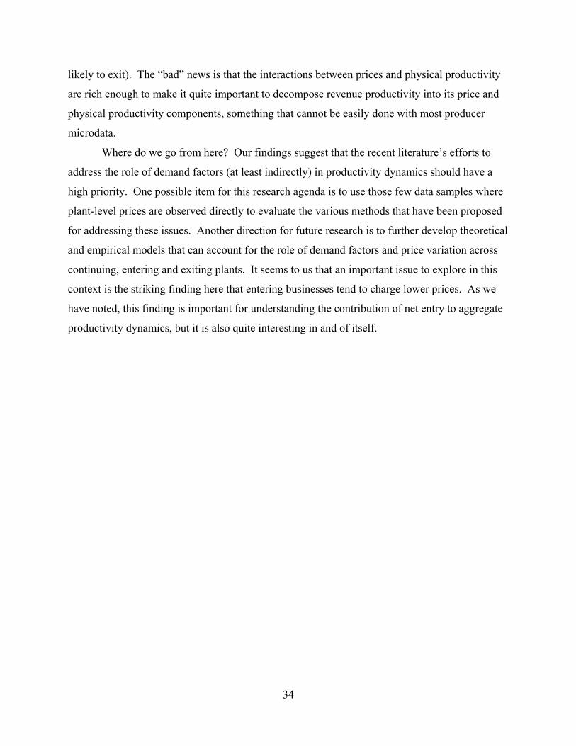
likely to exit). The “bad” news is that the interactions between prices and physical productivity
are rich enough to make it quite important to decompose revenue productivity into its price and
physical productivity components, something that cannot be easily done with most producer
microdata.
Where do we go from here? Our findings suggest that the recent literature’s efforts to
address the role of demand factors (at least indirectly) in productivity dynamics should have a
high priority. One possible item for this research agenda is to use those few data samples where
plant-level prices are observed directly to evaluate the various methods that have been proposed
for addressing these issues. Another direction for future research is to further develop theoretical
and empirical models that can account for the role of demand factors and price variation across
continuing, entering and exiting plants. It seems to us that an important issue to explore in this
context is the striking finding here that entering businesses tend to charge lower prices. As we
have noted, this finding is important for understanding the contribution of net entry to aggregate
productivity dynamics, but it is also quite interesting in and of itself.
34

References Abbott III, Thomas A. “Price Dispersion in U.S. Manufacturing: Implications for the
Aggregation of Products and Firms.” Center for Economic Studies Working Paper 92-3, 1992.
Aw, Bee Yan, Xiaomin Chen, and Mark Roberts. “Firm-Level Evidence on Productivity
Differentials and Turnover in Taiwanese Manufacturing,” Journal of Development Economics, October 2001.
Baily, Martin N., Charles Hulten, and David Campbell. “Productivity Dynamics in
Manufacturing Establishments,” Brookings Papers on Economic Activity: Microeconomics, 1992, 187-249.
Bartelsman, Eric J. and Mark Doms. “Understanding Productivity: Lessons from Longitudinal
Microdata.” Journal of Economic Literature, 38(3), 2000, 569-95. Davis, Steven J. and John Haltiwanger. “Wage Dispersion between and within U.S.
Manufacturing Plants, 1963-1986.” Brookings Papers on Economic Activity, Microeconomics 1991, 115-80.
De Loecker, Jan. “Product Differentiation, Multi-Product Firms and Structural Estimation of
Productivity.” Mimeo, 2005. Diewert, Erwin and Kevin Fox. “On Measuring the Contribution of Entering and Exiting Firms
to Aggregate Productivity Growth.” Mimeo, 2005. Dunne, Timothy and Mark Roberts. “Costs, Demand, and Imperfect Competition as
Determinants of Plant-Level Output Prices.” in Empirical Studies in Industrial Organization: Essays in Honor of Leonard W. Weiss, David Audretsch and John Siegfried (eds.), Kluwer Academic Publishers, 1992, 13-34.
Dunne, Timothy, Mark J. Roberts, and Larry Samuelson. “Patterns of Firm Entry and Exit in
U.S. Manufacturing Industries.” RAND Journal of Economics, 19(4), 1988, 495-515. Ericson, Richard and Ariel Pakes. “Markov-Perfect Industry Dynamics: A Framework for
Empirical Work.” Review of Economic Studies, 62(1), 1995, 53-82. Eslava, Marcela, John Haltiwanger, Adriana Kugler and Maurice Kugler. "The Effects of
Structural Reforms on Productivity and Profitability Enhancing Reallocation: Evidence from Colombia," Journal of Development Economics, 75(3), 2004, 333-371.
Eslava, Marcela, John Haltiwanger, Adriana Kugler and Maurice Kugler. "Employment and
Capital Adjustments After Factor Market Deregulation.", mimeo, 2005a.

Eslava, Marcela, John Haltiwanger, Adriana Kugler and Maurice Kugler. "Plant Survival, Market Fundamentals and Trade Liberalization", mimeo, 2005b.
Foster, Lucia, Haltiwanger, John, and C.J. Krizan. “Aggregate Productivity Growth: Lessons
from Microeconomic Evidence,” in New Developments in Productivity Analysis, editors: Edward Dean, Michael Harper and Charles Hulten, Chicago: University of Chicago Press, 2001.
Foster, Lucia, John Haltiwanger, and C.J. Krizan. “The Link Between Aggregate and Micro
Productivity Growth: Evidence from Retail Trade.” NBER Working Paper, 2002. Gorodnichenko, Yuriy. “What Do We Estimate in Production Function Regressions? Critique
and New Approaches.” Mimeo, 2005. Harper, Michael, Ernst R. Berndt, and David O. Wood. “Rates of Return and Capital
Aggregation using Alternative Rental Prices,” in Jorgenson, Dale W. and Ralph Landau (eds.), Technology and Capital Formation, MIT Press, 1989.
Hopenhayn, Hugo A. “Entry, Exit, and Firm Dynamics in Long Run Equilibrium.”
Econometrica, 60(5), 1992, 1127-50. Jovanovic, Boyan. “Selection and the Evolution of Industry.” Econometrica, 50(3), 1982, 649-
70. Katayama, Haijime, Shihua Lu, and James Tybout. “Why Plant-Level Productivity Studies are
Often Misleading, and an Alternative Approach to Interference.” NBER Working Paper 9617, 2003.
Klette, Tor Jakob and Zvi Griliches. “The Inconsistency of Common Scale Estimators When
Output Prices Are Unobserved and Endogenous.” Journal of Applied Econometrics, 11(4), 1996, 343-61.
Levinsohn, James and Amil Petrin, "Estimating Production Functions Using Inputs to Control
for Unobservables," Review of Economic Studies , 70(2), April, 2003, 317-342. Mairesse, Jacques and Jordi Jaumandreu. “Panel-Data Estimates of the Production Function and
the Revenue Function: What Difference Does it Make?” Mimeo, 2005. Melitz, Marc J. “Estimating Firm-Level Productivity in Differentiated Product Industries.”
Mimeo, Harvard University, 2000. Melitz, Marc J. “The Impact of Trade on Intra-Industry Reallocations and Aggregate Industry
Productivity.” Econometrica, 71(6), 2003, 1695-1725. Melitz, Marc J. and Gianmarco I. P. Ottaviano. “Estimating Firm-Level Productivity in
Differentiated Product Industries.” Mimeo, Harvard University, 2003.

Olley, G. Steven and Ariel Pakes. “The Dynamics of Productivity in the Telecommunications
Equipment Industry.” Econometrica, 64(6), 1996, 1263-1297. Roberts, Mark J. and Dylan Supina. “Output Price, Markups, and Producer Size.” European
Economic Review, 40(3-5), 1996, 909-21. Roberts, Mark J. and Dylan Supina. “Output Price and Markup Dispersion in Micro Data: The
Roles of Producer Heterogeneity and Noise.” in Advances in Applied Microeconomics, Vol. 9, Industrial Organization. Michael R. Baye (ed.), JAI Press, 2000.
Shea, John. “Instrument Relevance in Multivariate Linear Models: A Simple Measure,” The
Review of Economics and Statistics, 79(,2), May 1997, 348-352. Syverson, Chad. “Market Structure and Productivity: A Concrete Example.” Journal of Political
Economy, 112(6), 2004, 1181-1222. Syverson, Chad. “Prices, Spatial Competition, and Heterogeneous Producers: An Empirical
Test.” Mimeo, 2005. U.S. Bureau of Economic Analysis. “Redefinition of the BEA Economic Areas.” Survey of
Current Business, February 1995, pp.75-81. U.S. Bureau of Labor Statistics. “Trends in Multifactor Productivity: 1948-81.” Bulletin 2178.
Washington D.C., Government Printing Office, 1983. Van Biesebroeck, Johannes. “Robustness of Productivity Estimates.” NBER Working Paper
10303, 2004.

Table 1. Summary Statistics for Output, Price, and Productivity Measures
Correlations Variables Traditional
Output Revenue Output
Physical Output
Price
Traditional TFP
Revenue TFP
Physical TFP
Traditional Output
1.00
Revenue Output
0.99 1.00
Physical Output
0.98 0.99 1.00
Price
-0.03 -0.03 -0.19 1.00
Traditional TFP
0.19 0.18 0.15 0.13 1.00
Revenue TFP
0.17 0.21 0.18 0.16 0.86 1.00
Physical TFP
0.17 0.20 0.28 -0.54 0.64 0.75 1.00
Standard Deviations
Standard Deviations
1.03 1.03 1.05 0.18 0.21 0.22 0.26
Note: All values control for product-year effects. N = 17,699.

Table 2. Estimating Price Elasticities by Product
IV Estimation OLS Estimation
Product Price Coefficient(α1)
Income Coefficient
(α2)
Price Coefficient
(α1)
Income Coefficient
(α2)
Boxes -3.020.14 [0.61]
-0.03 0.02
-2.19 0.11
-0.03 0.02
Bread -3.090.30 [0.33]
0.12 0.04
-0.89 0.15
0.07 0.03
Carbon Black -0.520.27 [0.50]
-0.21 0.06
-0.57 0.19
-0.21 0.06
Coffee -3.630.51 [0.41]
0.22 0.08
-1.03 0.29
0.20 0.08
Concrete -5.930.29 [0.10]
0.13 0.01
-0.83 0.08
0.15 0.01
Hardwood Flooring -1.670.45 [0.61]
-0.20 0.14
-0.87 0.34
-0.24 0.13
Gasoline -1.421.58 [0.20]
0.23 0.04
-0.16 0.70
0.23 0.04
Block Ice -2.050.38 [0.32]
0.00 0.08
-0.63 0.17
0.16 0.06
Processed Ice -1.480.22 [0.37]
0.18 0.03
-0.70 0.13
0.16 0.03
Plywood -1.210.11 [0.89]
-0.23 0.06
-1.19 0.10
-0.23 0.06
Sugar -2.520.90 [0.15]
0.76 0.08
-1.04 0.32
0.72 0.07
Note: All regressions include a constant term and year effects. Standard errors in italics. Where applicable, Shea-corrected first-stage R2 are listed in brackets.

Table 3. Persistence of Productivity, Prices and Demand Shocks
Five-Year Horizon Implied One-Year Persistence Rates
Dependent Variable
Unweighted Regression
Weighted Regression
Unweighted Regression
Weighted Regression
Traditional TFP 0.249 0.011
0.303 0.011 0.757 0.788
Revenue TFP 0.277 0.012
0.306 0.011 0.774 0.789
Physical TFP 0.312 0.011
0.336 0.011 0.792 0.804
Price 0.365 0.010
0.366 0.011 0.817 0.818
Demand Shock 0.619 0.010
0.843 0.005 0.909 0.966
Note: Sample includes continuing establishments only. Weighted regressions are weighted by revenue. Regression results are coefficients on establishment’s five-year lag of dependent variable. Standard errors in italics.
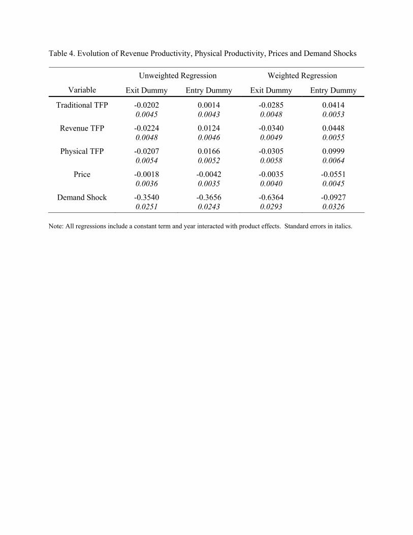
Table 4. Evolution of Revenue Productivity, Physical Productivity, Prices and Demand Shocks
Unweighted Regression Weighted Regression
Variable Exit Dummy Entry Dummy Exit Dummy Entry Dummy
Traditional TFP
-0.0202 0.0045
0.0014 0.0043
-0.0285 0.0048
0.0414 0.0053
Revenue TFP
-0.0224 0.0048
0.0124 0.0046
-0.0340 0.0049
0.0448 0.0055
Physical TFP
-0.0207 0.0054
0.0166 0.0052
-0.0305 0.0058
0.0999 0.0064
Price
-0.0018 0.0036
-0.0042 0.0035
-0.0035 0.0040
-0.0551 0.0045
Demand Shock -0.3540 0.0251
-0.3656 0.0243
-0.6364 0.0293
-0.0927 0.0326
Note: All regressions include a constant term and year interacted with product effects. Standard errors in italics.
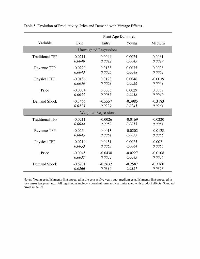
Table 5. Evolution of Productivity, Price and Demand with Vintage Effects
Plant Age Dummies
Variable Exit Entry Young Medium
Unweighted Regressions
Traditional TFP
-0.0211 0.0040
0.0044 0.0042
0.0074 0.0045
0.0061 0.0049
Revenue TFP
-0.0220 0.0043
0.0133 0.0045
0.0075 0.0048
0.0028 0.0052
Physical TFP
-0.0186 0.0050
0.0128 0.0053
0.0046 0.0056
-0.0039 0.0061
Price -0.0034 0.0033
0.0005 0.0035
0.0029 0.0038
0.0067 0.0040
Demand Shock
-0.3466 0.0218
-0.5557 0.0229
-0.3985 0.0245
-0.3183 0.0264
Weighted Regressions
Traditional TFP
-0.0211 0.0044
-0.0026 0.0052
-0.0169 0.0053
-0.0220 0.0054
Revenue TFP
-0.0264 0.0045
0.0013 0.0054
-0.0202 0.0055
-0.0128 0.0056
Physical TFP
-0.0219 0.0053
0.0451 0.0063
0.0025 0.0064
-0.0021 0.0065
Price -0.0045 0.0037
-0.0438 0.0044
-0.0227 0.0045
-0.0108 0.0046
Demand Shock
-0.6231 0.0266
-0.2632 0.0316
-0.2587 0.0321
-0.3760 0.0328
Notes: Young establishments first appeared in the census five years ago, medium establishments first appeared in the census ten years ago. All regressions include a constant term and year interacted with product effects. Standard errors in italics.

Table 6. Selection on Productivity or Profitability?
Specification: [1] [2] [3] [4] [5] [6] [7]
Unweighted Regressions
Traditional TFP -0.073 0.014
Revenue TFP -0.063 0.013
Physical TFP -0.040 0.012
-0.062 0.014
-0.034 0.012
Prices -0.021 0.018
-0.069 0.021
Demand Shock -0.047 0.003
-0.047 0.003
Weighted Regressions
Traditional TFP -0.055 0.012
Revenue TFP -0.062 0.011
Physical TFP -0.031 0.010
-0.059 0.012
-0.028 0.009
Prices -0.034 0.014
-0.078 0.017
Demand Shock -0.038 0.002
-0.038 0.002
Note: All specifications are probits of plant exit by next census of manufactures on plant-level values and include a full set of product-year interactions. Specifications 1 thru 5 are for each of our main variables of interest in isolation, while specifications 6 and 7 are for physical TFP jointly with prices or idiosyncratic demand measures. Standard errors in italics.
Table 7. Decomposition of Industry Productivity Growth Over Five-Year Horizons
Components of Decomposition (FHK/BHC) Productivity Measure
Total Growth Within Between Cross Entry Exit Net Entry
Traditional 2.31 0.91 -0.38 1.1 0.54 0.15 0.69
Revenue 5.09 3.38 -0.51 1.32 0.71 0.19 0.90
Physical 5.09 3.45 -0.40 0.70 1.22 0.12 1.34
Components of Decomposition (GR)
Within Between Entry Exit Net Entry
Traditional 2.31 1.46 0.15 0.44 0.26 0.70
Revenue 5.09 4.04 0.13 0.54 0.37 0.91
Physical 5.09 3.80 -0.07 1.04 0.31 1.35 Note: Decomposition of industry level productivity growth using equations (21) and (22) in text. The column labeled total reflects the average five-year productivity growth for the 1982-87 and the 1987-92 periods for the average (weighted) industry. The remaining columns all reflect the terms in the decomposition. Weights used in decompositions are revenue weights and then average revenue in beginning and end year for the industry is used to calculate the results for the average industry.

Data Appendix A.1. Defining Our Products As background to how we define our products, it is first necessary to understand the product coding scheme that Census uses. There are three types of codes that we highlight. First, Census codes flags products from administrative records (AR) sources. We exclude all of these AR products from our analysis. (Including in our measures of PPSR since it is obviously not possible to assign these AR products to a single 7-digit code.) Second, Census uses balancing codes to correct cases in which the sum of the total value of shipments of reported individual products does not sum to the reported total value of shipments. Census identified these balancing codes using special suffixes for the product codes in every census year except in 1987. Where balancing codes are identified, they have been deleted. Finally, Census collects data on receipts for contract work, miscellaneous receipts, and resales of products. These products are excluded from our calculations of PPSR (again, because it is obviously not possible to assign these AR products to a single 7-digit code). As a final exclusion, we did not include any products in that have a negative value since these are presumably balancing codes. The precise definitions of our eleven products are listed below (with 7-digit product codes in parentheses). Boxes is defined as the sum of boxes classified by their end use and boxes classified by their materials. Boxes classified by end use are: food and beverages (2653012), paper and allied products (2653013), carryout boxes for retail food (2653014 category starts in 1987) glass, clay, and stone products (2653015), metal products, machinery, equipment, and supplies except electrical (2653016), electrical machinery, equipment, supplies, and appliances (2653018), chemicals and drugs, including paints, varnishes, cosmetics, and soap (2653021), lumber and wood products, including furniture (2653029), and all other ends uses not specified above (2653029 in 1977 and 1982, 2653030 in 1987). Boxes classified by their materials are: solid fiber (2653051), corrugated paperboard in sheets and rolls, lined and unlined (2653067), and corrugated and solid fiber pallets, pads and partitions (2653068). The physical data for boxes is measured in short tons. Bread is defined as one 7-digit product, white pan bread (2051111), until 1992 when it was split into two products white pan bread, except frozen (2051121) and frozen white pan bread (2051122). The physical data for bread is measured in thousands of pounds. Carbon Black is defined as one 7-digit product, carbon black (2895011 in 1977, 2895000 thereafter). The physical data for carbon black is measured in thousands of pounds. Coffee is the sum of whole bean (2095111), ground and extended yield (2095117 and 2095118 in 1982 and 2095115 thereafter), and ground coffee mixtures (2095121). The physical data for coffee is measured in thousands of pounds. Concrete is defined as one 7-digit product, ready-mix concrete (3273000), over our entire sample. Some of the products coded as 3237300 in 1987 were in fact census balancing codes and thus were deleted from our sample. The physical data for concrete is measured in thousands of cubic yards.

Flooring is defined as one 7-digit product, hardwood oak flooring (2426111), over our entire sample. The physical data for flooring is measured in thousands of board feet. Gasoline is defined as one 7-digit product, motor gasoline (2911131), over our entire sample. The physical data for gasoline is measured in thousands of barrels. Block Ice is defined as one 7-digit product, can or block ice (2097011), over our entire sample. The physical data for block ice is measured in short tons. Processed Ice is defined as one 7-digit product, cubed, crushed, or other processed ice (2097051), over our entire sample. The physical data for processed ice is measured in short tons. Plywood is defined as one 7-digit product, hardwood plywood (2435100), over 1977-1987. Starting in 1992, plywood is the sum of veneer core (2435101), particleboard core (2435105), medium density fiberboard core (2435107), and other core (2435147). The physical data for plywood is measured in thousands of square feet surface measure. Sugar is defined as one 7-digit product, raw cane sugar (2061011), over our entire sample. The physical data for sugar is measured in short tons. A.2 Characteristics of Establishments by Product
In this section we briefly characterize some of the relevant properties of the establishments that produce our products. Table A.1 shows characteristics of the sample by product. The first five columns show the number of establishments in our sample by year for each product. The second to last column shows the revenue shares of each product. Revenue is the weight used in our weighted regressions. Concrete clearly dominates our sample in terms of the number of establishments, however, gasoline dominates our sample in terms of the revenue share The last column of the table shows the mean log income for each product in our sample. Concrete has the highest mean log income while carbon black has the lowest. Table A.2 shows the entry and exit rates by product for the data pooled over all available years. Entry rates range from a low of 3.9 for sugar to a high of 26.6 for concrete, while exit rates range from a low of 9.0 for gasoline and to a high of 27.7 for processed ice. Some products appear to be in a period of retrenchment or consolidation. Sugar for example, has a very low entry rate (3.9) but a high exit rate (17.0). The number of plants in the Sugar and Confectionary Products industry (2061) has fallen from 66 in 1977 to 39 in 1997. Other products appear to simply have a high degree of churning. For example, concrete and both types of ice products all have entry rates and exit rates that exceed 20 percent. The number of establishments in Ready-Mix Concrete (3273) industry increases over our sample period, while the number of establishments in the Block and Processed Ice industry (2097) falls somewhat over our sample (from 675 establishments in 1977 to 582 establishments in 1997).

Table A.1: Characteristics of the Sample by Product
Number of Observations
Product 1977 1982 1987 1992 1997 Revenue
Share (%) Mean (log)
Income
Boxes 936 905 1045 NA NA 6.0 17.4
Bread 195 142 110 92 92 2.2 17.0
Carbon Black 31 23 22 21 18 0.6 16.2
Coffee 61 84 79 77 77 4.5 18.0
Concrete 2184 3316 3236 3427 NA 6.0 17.1
Hardwood Flooring 8 10 16 25 24 0.2 16.7
Gasoline 99 99 94 95 71 78.6 17.1
Block Ice 40 43 26 23 10 0.0 16.9
Processed Ice 87 155 144 NA NA 0.1 16.8
Plywood 71 68 42 42 37 0.6 16.5
Sugar 40 36 30 35 26 1.1 16.6 Note: Revenue share is the share in total sample revenue for all years pooled. Mean log income is for plants’ corresponding Economic Areas (see text for details) based on data pooled over all years.

Table A.2: Entry and Exit Rates by Product
Products Entry Rates Exit Rates
All Products 22.3 19.6
By Product:
Boxes 12.4 12.2
Bread 7.6 18.9
Carbon Black 4.8 13.4
Coffee 9.1 15.6
Concrete 26.6 21.8
Hardwood Flooring 18.7 11.9
Gasoline 4.2 9.0
Block Ice 24.5 26.5
Processed Ice 23.1 27.7
Plywood 7.4 10.3
Sugar 3.9 17.0


