

C h a p t e r 5
SELF-ORGANIZATION OF SPATIAL SOLITONS
5.1. INTRODUCTION
In this chapter we present experimental results on the self-organization of spatial solitons in
a self-focusing nonlinear medium. We have observed the emergence of order, self
organization and a transition to a chaotic state. Nonlinear interactions between light and
matter can lead to the formation of spatial patterns and self-trapped optical beams.
Modulation instability is responsible for the spontaneous formation of optical patterns,
which have been observed both with coherent and incoherent light [1,2]. Under certain
conditions, self-trapped optical beams (spatial solitons) can be generated through the
interplay between diffraction and nonlinear effects [3-5]. Self-trapped light filaments have
been observed in materials with quadratic [6] and cubic [7] (Kerr) optical nonlinearities.
Spatial solitons can interact through collisions [8,9], which opens the possibility of using
them to perform computations [10]. Optical filaments can also act as waveguides, and it
was recently shown that in liquid crystals they can be steered using an applied voltage [11].
Applications involving the use of spatial solitons will most likely require large numbers of
them; however, the effects of the interactions between large numbers of filaments remain
largely unexplored. Here we report the observation of self-organization of spatial solitons
into a periodic array and the later breakdown of the periodicity. The array initially forms
with a period that depends on the intensity of the illuminating beam. If the filaments are
formed too closely they rearrange themselves into an array with a larger more stable period.
This result has implications for the density with which solitons can be packed both for
information processing and communication applications.
86

A light pulse propagating in a nonlinear Kerr medium will come to a focus if its power is
above a critical value. If the pulse power is much higher than the critical power then the
optical beam will break up into multiple filaments [12-14]. Each filament will contain
approximately the critical power, defined as [15]:
20
22
8)61.0(
nnPcr
λπ= . (5.1)
where λ is the laser wavelength in vacuum, n0 is the linear refractive index of the material
and n2 is the material constant that gives the strength of the Kerr nonlinearity in units of
inverse light intensity. We have used carbon disulfide as the nonlinear material (n0 = 1.6, n2
= 3x10-15cm2/W [16]), which has a critical power of 190 kW for our laser wavelength of
800 nm.
5.2 EXPERIMENTAL SETUP
The experimental setup is shown in Figure 5.1. A Ti:Sapphire laser amplifier system is
used to generate 150-femtosecond pulses with a maximum energy of 2 mJ. The standard
deviation in laser pulse energy from shot-to-shot is 3%. The laser is run at the maximum
energy level to achieve maximum stability, and neutral density filters are used to adjust the
pulse energy in the experiment. Each pulse from the laser is split into pump and probe
pulses. The pump pulse propagates through a 10 mm glass cell filled with carbon disulfide
(CS2). The beam profile of the pump at the exit of the glass cell is imaged onto a CCD
camera (CCD 1) with a magnification factor of 5. A cylindrical lens (focal length = 10 cm)
focuses the pump beam into a line approximately 3 mm inside the medium. The line focus
generates a single column of filaments. We studied the filamentation process using
Femtosecond Time-resolved Optical Polarigraphy (FTOP) [17]. This technique uses the
transient birefringence induced in the material through the Kerr effect to capture the beam
profile. The probe pulse propagates in a direction perpendicular to the pump. The presence
of the pump induces a transient birefringence proportional to the intensity of the pulse. The
87

trajectory of the pump pulse can be captured with high temporal resolution by monitoring
the probe pulse through cross polarizers. In our experimental setup (Fig. 5.1), the pump is
polarized in the vertical direction and the probe is polarized at 45 degrees with respect to
the pump’s polarization. After the probe traverses the nonlinear medium it goes through an
analyzer (polarizer at -45 degrees) and is imaged on a second CCD camera (CCD 2) with a
magnification factor of 6. Light from the probe reaches the detector only if the probe
temporally and spatially overlaps with the pump inside the nonlinear material. A delay line
is used to synchronize the arrival of pump and probe pulses, and allows us to observe the
pump at different positions along the direction of propagation.
Figure 5.1. FTOP setup. The pump pulse is focused in the material with a cylindrical
lens to generate a single column of filaments. The beam profile at the output is
imaged on CCD 1. The probe pulse goes through a variable delay line, a polarizer
and analyzer and is imaged on CCD.
Polarizer
Analyzer CCD 1
Delay line
Pump pulse
Probe pulse
CCD 2
Imaging lens
mirror
Cylindrical lens
CS2
Polarizer
Analyzer CCD 1
Delay line
Pump pulse
Probe pulse
CCD 2
Imaging lens
mirror
Cylindrical lens
Imaging lens
mirror
Cylindrical lens
CS2
88

5.3. EXPERIMENTAL RESULTS
5.3.1. Beam profile and instabilities as a function of pulse energy
Figure 5.2 shows the beam profile of the pump beam at the output of the CS2 cell (CCD 1
in Fig. 1) as a function of pump pulse power. In the absence of nonlinearity the incident
cylindrical beam would diverge to a width of 200 µm as it propagates to the output surface.
For a pulse power equal to 12 times the critical power (P = 12 Pcr, Fig. 5.2a), self focusing
and diffraction nearly balance each other, and the output beam width is approximately the
same as for the input. For higher pulse power the beam self focuses into an increasingly
thinner line (Figs. 5.2b and 5.2c) with a minimum width equal to 16 μm for P = 80 Pcr. It is
clearly evident in Fig. 5.2c that modulation instability has generated self focusing in the
orthogonal direction as well. For P > 100 Pcr, the beam breaks up into individual filaments
(Fig. 5.2d-e). The filaments are seeded by small variations in the input beam and are stable
in location and size to small variations in the input energy. In other words, the pattern of
filaments is repeatable from shot to shot as long as the illuminating beam profile is kept
constant. The diameter of the filaments is approximately 12 μm and does not change when
the energy is increased, while the number of filaments increases with power. When P >
250 Pcr, the output beam profile becomes unrepeatable and the filaments start to fuse into a
continuous line (Fig 2f-h). We will explain the origin of this instability later on. Part of the
energy is scattered out of the central maximum into side lobes. The mechanism responsible
for the formation of the side lobes is the emission of conical waves [18,19] during the
formation of the filaments. The diameter of the filaments initially decreases until it reaches
a stable condition; at this point some of the energy is released through conical emission
while the rest of the energy is trapped in the filament [20].
89

Figure 5.2. Beam profile of the pump pulse at the output of the CS2 cell. The power
increases from left to right: a) P = 12Pcr, b) 40Pcr, c) 80Pcr, d) 170Pcr, e) 250Pcr, f)
390Pcr, g) 530Pcr, h) 1200Pcr. The size of each image is 0.36 mm (h) x 0.89 mm (v).
Video 5.1 and Video 5.2 show how the shot-to-shot fluctuations in the pulse energy affect
the beam profile at the output of the cell. For each video, ten images were captured with the
same experimental conditions and compiled into a movie clip, the only variable being the
fluctuations in the laser pulse energy. For a pulse with a power of 170 Pcr the output beam
profile is stable (Video 5.1). There are only small changes in the position of the filaments
while the overall pattern of filaments remains constant. Filaments that appear close to each
other seem to be the most sensitive to the energy fluctuations. If the power is increased to
390 Pcr the beam profile at the output becomes unrepeatable (Video 5.2). The position of
the filaments varies greatly from shot to shot and the central line bends differently for each
shot.
(a) (g)(f)(e)(d)(c)(b) (h)
200μm
(a) (g)(f)(e)(d)(c)(b) (h)
200μm200μm
90

Video 5.1. Movie of changes in the beam profile as a result of fluctuations in the
pulse energy for P = 170 Pcr (78.5 KB). The image area is 0.36 mm (h) x 0.89 mm (v).
Video 5.2. Movie of changes in the beam profile as a result of fluctuations in the
pulse energy for P = 390 Pcr (113 KB). The image area is 0.36 mm (h) x 0.89 mm (v).
91

Increasing the pulse energy causes the beam to self-focus faster and break up into filaments
earlier. As shown above, further increasing the energy causes the beam to become unstable.
For low energy levels the beam profile remains uniform, but as the energy is increased the
beam breaks up into a periodic array of filaments. We have measured the beam profile at a
fixed distance from the cell entrance for eight different pulse energies. The beam profile is
captured using the FTOP setup with a fixed delay. Figure 5.3a shows a cross section of the
beam profile at a distance of 2.5 mm inside the cell for pulse power of P = 250 Pcr, 390 Pcr,
530 Pcr, 790 Pcr, 1200 Pcr, 1700 Pcr, 2700 Pcr, 3800 Pcr. Higher power levels are necessary
to observe filaments after a distance of 2.5 mm, as opposed to 10 mm in Figure 5.2. Figure
5.3b shows the Fourier transform of the beam cross sections in Figure 5.3a. The central
peak (DC component) in the Fourier transform is blocked to visualize the secondary peaks.
For P = 250 Pcr, no filaments are observed as the beam remains uniform after 2.5 mm.
Note that for this power the beam completely breaks up into filaments after 10 mm (Fig.
5.2e). As the power is increased between 390 Pcr and 790 Pcr an increasing number of
filaments appears in a periodic array. The periodicity is clearly visible in the Fourier
transform; a peak appears that corresponds to the spacing between the filaments (~ 20 µm).
The emergence of periodicity in the beam pattern is discussed in the following section.
When the power is increased above 1200 Pcr the periodicity starts to disappear. The beam is
no longer uniform but there is no clear indication of the formation of filaments. This state
corresponds to the patterns in Figure 2f-h, where the beam profile becomes unstable.
92

Figure 5.3. Beam profile inside the cell as a function of power. (a) Cross sections of
the beam profile at 2.5 mm inside the cell for pulse power P/Pcr = 250, 390, 530, 790,
1200, 1700, 2700, 3800. The cross sectional plots for different powers are displaced
vertically for visual clarity. The lowest power is displaced at the bottom. The peaks
correspond to regions of higher intensity (filaments). (b) Fourier transform of the
plots in (a). The peaks represent the periodicity of the arrays of filaments. A strong
central peak (DC component) is zeroed to display the secondary peaks.
5.3.2. Spatial evolution of the beam and self-organization
Video 5.3 shows the filamentation process for a pulse with P = 390 Pcr. The pulse
propagation inside the material is captured from 2 mm to 4 mm from the cell entrance
using the FTOP setup. The width of the image of the pulse on the CCD camera (CCD 2 in
Fig. 5.1) depends on the pulse duration and the time response of the material. CS2 has both
a very fast (femtosecond) electronic time response and a slower (picosecond) molecular
response. In our experiments, the time response at the leading edge of the signal is
essentially instantaneous, and the resolution is determined by the pulse duration (150
-110 -55 0 55 110fx (1/mm)
-110 -55 0 55 110-110 -55 0 55 110fx (1/mm)
0 0.1 0.2-0.1-0.2x (mm)
0 0.1 0.2-0.1-0.2x (mm)
(a) (b)
3800
2700
1700
1200
790
530
390
250-110 -55 0 55 110
fx (1/mm)-110 -55 0 55 110-110 -55 0 55 110
fx (1/mm)0 0.1 0.2-0.1-0.2
x (mm)0 0.1 0.2-0.1-0.2
x (mm)
(a) (b)
3800
2700
1700
1200
790
530
390
250
93

femtoseconds). On the trailing edge of the signal a slower decay time of approximately 1.5
picoseconds is observed, which is consistent with the time constant for the molecular
response of the material. The movie clip in Video 3 shows the propagation of a pulse with a
spatial profile that is initially uniform. The movie is compiled from multiple pump-probe
experiments by varying the delay of the probe pulse. As the beam propagates the intensity
modulation increases until the beam breaks up into filaments. The light is trapped in the
filaments, which continue to propagate with a constant diameter for several millimeters.
Video 5.3. Pulse propagation inside CS2 from 2 mm to 4 mm from the cell entrance
for a pulse power of 390 Pcr. An initially uniform beam breaks up into stable filaments
(258 KB). The image size is 2.4 mm (h) x 1.6 mm (v).
Figure 5.4 shows the trajectory of the beam obtained in the FTOP setup for pulses with P =
390 Pcr (a) and 1200 Pcr (c), from a distance of 0.5 cm to 5 cm from the cell entrance. The
trajectory is obtained by numerically combining multiple pump-probe images of the pulse
at different positions as it traverses the material. The 1-D Fourier transforms of the beam
profile are calculated and displayed in Figure 5.4b and 5.4d for each position along the
propagation direction. The peaks in the Fourier transform correspond to the periodicity in
the positions of the filaments. The central peak (DC component) in the Fourier transform is
94

blocked to improve the contrast in the image. Periodic changes in the amplitude of the
peaks along the propagation direction are artifacts due to the sampling of the beam profile
in the experiments.
The pulse with lower power (Fig. 5.4a) breaks up into filaments at a distance of 2.9 mm
into the material, while the pulse with higher power (Fig. 5.4c) breaks up at 1.5 mm from
the cell entrance. The Fourier transform in Fig. 4b clearly shows how a periodicity emerges
during the filamentation process. The filaments are created in a regular array and propagate
undisturbed for several millimetres. The spacing between the filaments is approximately 40
µm, about four times the diameter of the filaments. If the pulse energy is higher (Fig. 5.4d)
the array of filaments initially forms with a higher spatial frequency. The period then
increases from 22 µm to 33 µm as the filaments propagate. After 5 mm the sharp peaks
visible in the Fourier transform start to fan out. The gradual loss of the periodicity after 5
mm corresponds to a decline in the number of filaments. We attribute the change in the
period of the soliton array primarily to the interactions between nearby filaments. These
interactions cause filament fusion and conical emission, redirecting some of the energy
away from the main line of solitons. The filaments then continuously rearrange themselves
in a sparser grid. The interactions depend on the relative phase of the filaments. Filaments
of the same phase will attract while out-of-phase neighboring filaments will repel. The
phase of individual filaments is determined by the initial condition (the illuminating beam)
but also by the accumulated phase along the propagation path with linear and nonlinear
contributions. Slight intensity or angle changes can lead to large accumulated phase
differences. We believe that this effect is responsible for the onset of the chaotic behaviour
we observe.
95

Figure 5.4. Pulse trajectories and 1-D Fourier transforms. (a,c) The trajectory of the
pulse is reconstructed by digitally adding up the FTOP frames for different positions
of the pulse. Each separate image corresponds to frames taken for a fixed position of
CCD camera. The camera was moved laterally to capture the beam profile farther
along inside the cell. The pulse power is 390Pcr in (a) and 1200Pcr in (c). (b,d) Show
the 1-D Fourier transforms of the filamentation patterns in (a) and (c), respectively.
The central component is blocked to visualize higher frequencies.
(a)
(b)
(c)
(d)
0.5 1 2 3 4 5 (mm)
(a)
(b)
(c)
(d)
0.5 1 2 3 4 5 (mm)
(a)
(b)
(c)
(d)
0.5 1 2 3 4 5 (mm)0.5 1 2 3 4 5 (mm)
96
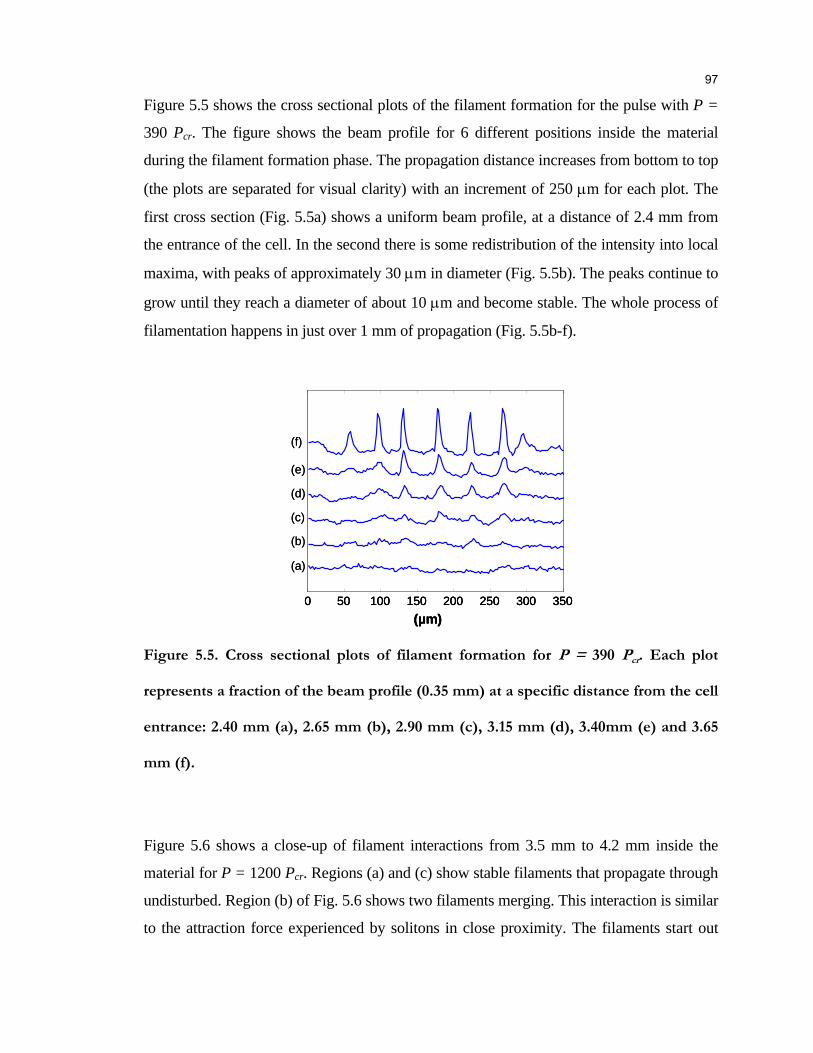
Figure 5.5 shows the cross sectional plots of the filament formation for the pulse with P =
390 Pcr. The figure shows the beam profile for 6 different positions inside the material
during the filament formation phase. The propagation distance increases from bottom to top
(the plots are separated for visual clarity) with an increment of 250 μm for each plot. The
first cross section (Fig. 5.5a) shows a uniform beam profile, at a distance of 2.4 mm from
the entrance of the cell. In the second there is some redistribution of the intensity into local
maxima, with peaks of approximately 30 μm in diameter (Fig. 5.5b). The peaks continue to
grow until they reach a diameter of about 10 μm and become stable. The whole process of
filamentation happens in just over 1 mm of propagation (Fig. 5.5b-f).
Figure 5.5. Cross sectional plots of filament formation for P = 390 Pcr. Each plot
represents a fraction of the beam profile (0.35 mm) at a specific distance from the cell
entrance: 2.40 mm (a), 2.65 mm (b), 2.90 mm (c), 3.15 mm (d), 3.40mm (e) and 3.65
mm (f).
Figure 5.6 shows a close-up of filament interactions from 3.5 mm to 4.2 mm inside the
material for P = 1200 Pcr. Regions (a) and (c) show stable filaments that propagate through
undisturbed. Region (b) of Fig. 5.6 shows two filaments merging. This interaction is similar
to the attraction force experienced by solitons in close proximity. The filaments start out
0 50 100 150 200 250 300 350(µm)
(a)
(b)
(c)
(d)
(e)
(f)
0 50 100 150 200 250 300 350(µm)
0 50 100 150 200 250 300 350(µm)
(a)
(b)
(c)
(d)
(e)
(f)
97
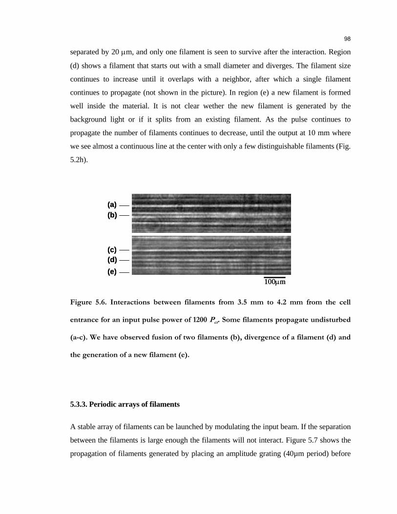
separated by 20 μm, and only one filament is seen to survive after the interaction. Region
(d) shows a filament that starts out with a small diameter and diverges. The filament size
continues to increase until it overlaps with a neighbor, after which a single filament
continues to propagate (not shown in the picture). In region (e) a new filament is formed
well inside the material. It is not clear wether the new filament is generated by the
background light or if it splits from an existing filament. As the pulse continues to
propagate the number of filaments continues to decrease, until the output at 10 mm where
we see almost a continuous line at the center with only a few distinguishable filaments (Fig.
5.2h).
Figure 5.6. Interactions between filaments from 3.5 mm to 4.2 mm from the cell
entrance for an input pulse power of 1200 Pcr. Some filaments propagate undisturbed
(a-c). We have observed fusion of two filaments (b), divergence of a filament (d) and
the generation of a new filament (e).
5.3.3. Periodic arrays of filaments
A stable array of filaments can be launched by modulating the input beam. If the separation
between the filaments is large enough the filaments will not interact. Figure 5.7 shows the
propagation of filaments generated by placing an amplitude grating (40µm period) before
100μm
(a)(b)
(c)(d) (e)
100μm
(a)(b)
(c)(d) (e)
98

the entrance of the cell. The input power is P = 200 Pcr. Filaments form very quickly and
propagate undisturbed (Fig. 5.7a). The 1-D Fourier transform in Fig. 5.7b shows that the
period induced by the grating does not change with propagation. Figure 5.7c shows the
array of filaments at the output face of the cell (10mm propagation). The propagation
distance of the filaments in this case is limited by the cell length. The modulation of the
beam amplitude speeds up the formation of the filaments, while the input energy ensures
the stability. Most of the available energy is trapped in the filaments; no light was detected
outside of the filaments. The energy in each filament can be estimated from the total energy
and the number of filaments. Each filament carries approximately four times the critical
power (4 Pcr).
Figure 5.7. Propagation of a pulse with a periodic beam profile (a) The trajectory of
the pulse is reconstructed by digitally adding up the FTOP frames for different
positions of the pulse. (b) 1-D Fourier transforms of the filamentation patterns in (a).
The central component is blocked to visualize higher frequencies. (c) Image of the
beam profile at the output of the cell after 10 mm of nonlinear propagation.
We have also generated 2-D arrays of filaments. The cylindrical lens is removed from the
setup for this experiment, so the input intensity is decreased. The input beam (5 mm
0.5 1 2 3 4 5 (mm)
40 μm
(a)
(b)
(c)
0.5 1 2 3 4 5 (mm)0.5 1 2 3 4 5 (mm)
40 μm40 μm
(a)
(b)
(c)
99
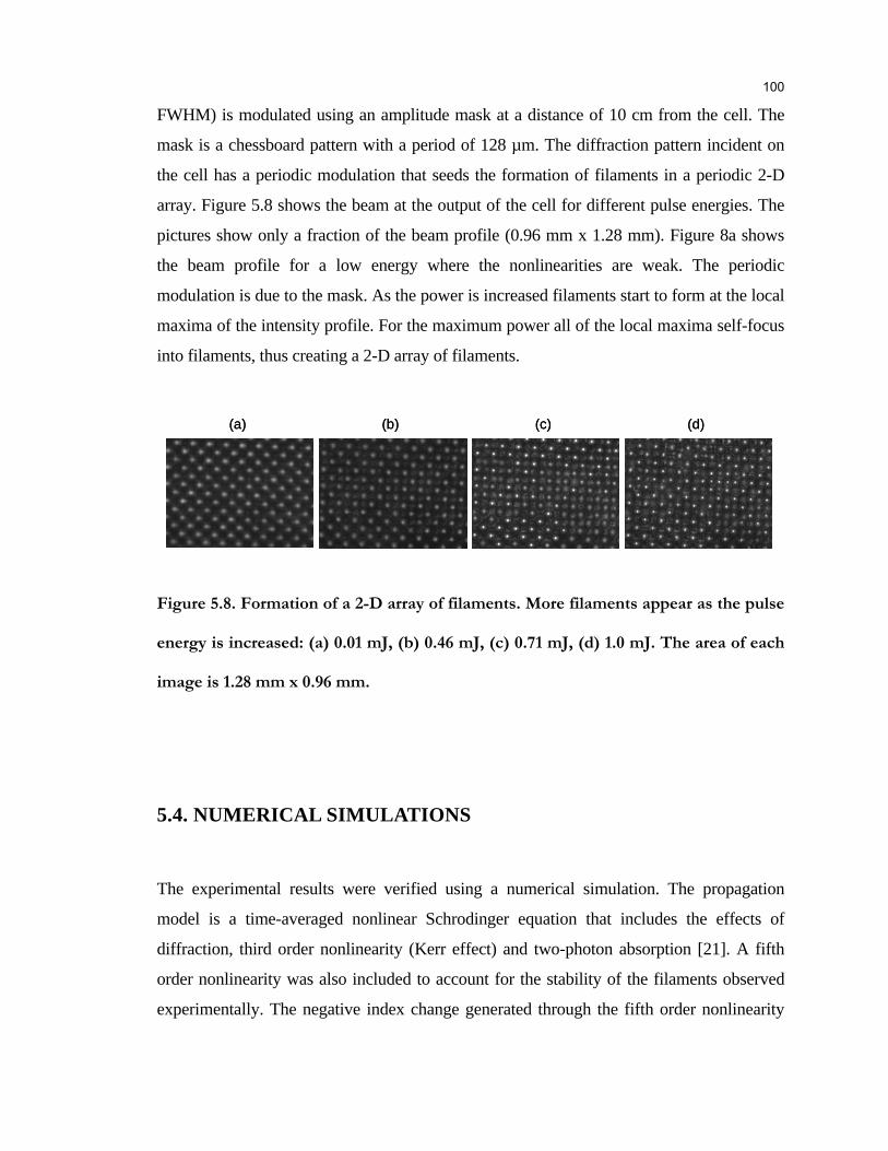
FWHM) is modulated using an amplitude mask at a distance of 10 cm from the cell. The
mask is a chessboard pattern with a period of 128 µm. The diffraction pattern incident on
the cell has a periodic modulation that seeds the formation of filaments in a periodic 2-D
array. Figure 5.8 shows the beam at the output of the cell for different pulse energies. The
pictures show only a fraction of the beam profile (0.96 mm x 1.28 mm). Figure 8a shows
the beam profile for a low energy where the nonlinearities are weak. The periodic
modulation is due to the mask. As the power is increased filaments start to form at the local
maxima of the intensity profile. For the maximum power all of the local maxima self-focus
into filaments, thus creating a 2-D array of filaments.
Figure 5.8. Formation of a 2-D array of filaments. More filaments appear as the pulse
energy is increased: (a) 0.01 mJ, (b) 0.46 mJ, (c) 0.71 mJ, (d) 1.0 mJ. The area of each
image is 1.28 mm x 0.96 mm.
5.4. NUMERICAL SIMULATIONS
The experimental results were verified using a numerical simulation. The propagation
model is a time-averaged nonlinear Schrodinger equation that includes the effects of
diffraction, third order nonlinearity (Kerr effect) and two-photon absorption [21]. A fifth
order nonlinearity was also included to account for the stability of the filaments observed
experimentally. The negative index change generated through the fifth order nonlinearity
(a) (b) (c) (d)(a) (b) (c) (d)
100
balances the positive Kerr index change. A complete simulation of the spatial and temporal
profile of the nonlinear pulse propagation requires very fine sampling in three spatial
dimensions and time. We assume in our model that the temporal profile of the pulse is
constant, which allows us to calculate the beam evolution with good spatial resolution. We
have shown in Chapter 4 that this model provides a good approximation to the propagation
of femtosecond pulses in CS2. The light propagation is calculated assuming a scalar
envelope for the electric field, which is slowly varying along the propagation direction z.
The evolution of the scalar envelope is given by the equation:
( ) ( ) AAAAnikAAnikAyxkn
idzdA 24
42
22
2
2
2
02β−−+⎟⎟
⎠
⎞⎜⎜⎝
⎛∂∂
+∂∂
= (5.2)
A(x,y,z,T) is the complex envelope of the electric field, λπ2
=k , λ = 800nm, n0 = 1.6, n2 =
3x10-15cm2/W [16], n4 = -2x10-27cm4/W2, β = 4.5x10⁻¹³ cm/W [21]. The first term on the
right-hand side accounts for diffraction, the second is Kerr self-focusing (third-order
nonlinearity), the third term accounts for the fifth-order nonlinearity and the last term
represents for two-photon absorption. Linear absorption is negligible at the wavelength
used in the experiments. The equation is solved numerically using the Split-step Fourier
method.
The two-photon absorption term affects the propagation only for the highest intensity levels
and does not significantly change the qualitative behaviour observed in the simulations.
The fifth-order nolinearity (n4) is the mechanism responsible for the generation of stable
light filaments. Since we could not find experimentally measured values of n4, in the
simulation we have assigned it the value that gave the best match with the experimental
results. The stabilization of the filaments can also be caused by a negative index change
due to the plasma generation. If the light intensity is high enough a plasma can be created
through multiphoton absorption. However, the intensity of the filaments is well below the
threshold for plasma generation [20]; therefore multiphoton ionization does not play a
significant role in the filament dynamics and does not need to be included in the
simulations.
101

The input beam for the simulation is generated using the image of the beam in Fig. 5.2a.
The square root of the measured intensity profile is used as the amplitude of the input light
field, and a phase profile is added to simulate the phase of the focused beam at the entrance
of the cell. The simulated field is a good approximation to the experimental input beam and
has a similar noise profile.
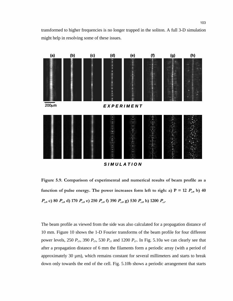
The model in equation 5.2 was used to numerically calculate the output beam profile after
propagating through 10 mm of CS2. Figure 5.9 shows a comparison of the numerical and
experimental results. The simulation follows the experimental results very closely during
the self-focusing stage (Fig. 5.9a-c). The beam self-focuses into a line of decreasing width
as the power is increased. There is also good agreement between simulation and
experiment when the beam breaks up into filaments (Fig. 5.9d-e). The number of filaments
is similar, and in both cases the filaments release some energy through conical emissions.
The difference in the spacing of the filaments is discussed below. Up to this point the
behaviour observed in the simulation is very similar to the experiments; however, the
simulation does not capture the behaviour of the beam in the chaotic stage (Fig. 5.9f-h). In
the experiments some energy is lost and the filaments disappear. A central bright line
remains and is surrounded by side-lobes that propagate away from the center. For the
highest power level new filaments appear in the side-lobes. The simulation shows different
behaviour, as more filaments appear in the central line and then start moving away. In the
numerical results the array becomes unstable as the density of the filaments increases and
some of the filaments get deflected through their mutual interactions; however, only some
of the filaments disappear while a lot of them survive. In fact, in the simulations most of
the energy is trapped in the filaments, even for the highest power levels.
The loss seems to be a key element in the discrepancy between experiment and simulation.
The only source of loss in the simulation is two-photon absorption, which does not
dissipate enough energy when compared to the experiment. It is not clear what causes the
energy loss in the experiments. Another source of error is in the temporal domain that is
neglected in the simulations. The spectral content of the solitons increases as they
propagate, which is ignored in the simulation. It is possible that the energy that is
102
transformed to higher frequencies is no longer trapped in the soliton. A full 3-D simulation
might help in resolving some of these issues.
Figure 5.9. Comparison of experimental and numerical results of beam profile as a
function of pulse energy. The power increases form left to righ: a) P = 12 Pcr, b) 40
Pcr, c) 80 Pcr, d) 170 Pcr, e) 250 Pcr, f) 390 Pcr, g) 530 Pcr, h) 1200 Pcr.
The beam profile as viewed from the side was also calculated for a propagation distance of
10 mm. Figure 10 shows the 1-D Fourier transforms of the beam profile for four different
power levels, 250 Pcr, 390 Pcr, 530 Pcr and 1200 Pcr. In Fig. 5.10a we can clearly see that
after a propagation distance of 6 mm the filaments form a periodic array (with a period of
approximately 30 µm), which remains constant for several millimeters and starts to break
down only towards the end of the cell. Fig. 5.10b shows a periodic arrangement that starts
200μm
(a) (g)(f)(e)(d)(c)(b) (h)
E X P E R I M E N T
S I M U L A T I O N
200μm200μm
(a) (g)(f)(e)(d)(c)(b) (h)
E X P E R I M E N T
S I M U L A T I O N
103

with a slightly smaller period before settling to a period of 30 µm. For the input power in
Fig. 5.10c the filaments initially form with a period of 16 µm after a propagation distance
of 3 mm. As the light propagates to a distance of 6 mm the period increases to 25 µm, and
after this point the period seems to continue to increase but the peaks in the Fourier
transform start to fan out as the array of filament loses its periodicity. For the highest
energy level (Fig. 5.10d) multiple peaks appear in the Fourier transform, with a trend
towards smaller spatial frequencies with increasing propagation distance. At this level no
clear periodicity is observed in the simulations. The behavior observed in the simulations is
very similar to that of the experimental results. In both cases order (periodicity) emerges,
evolves and eventually dissipates. In the simulations the filaments form with a smaller
period and the filamentation distance is longer. We attribute these differences to the lack of
knowledge of the exact initial conditions (beam intensity and phase), approximations made
in the numerical model and uncertainties in the constants used for the simulation.
Figure 5.10. 1-D Fourier transforms for numerically calculated beam propagation.
The beam propagation is numerically calculated for four different power levels a) P =
0 10 mm
(a)
(c)
(b)
(d)
0 10 mm0 10 mm
(a)
(c)
(b)
(d)
104

250 Pcr, b) 390 Pcr, c) 530 Pcr, d) 1200 Pcr. A 1-D Fourier transform on the side view
of the beam profile is calculated for each along the propagation direction. The total
distance is 10 mm. The central peak (DC component) in the Fourier transform is
blocked to improve the contrast in the image.
5.5. SUMMARY
We have observed the emergence of order, self organization and a transition to a chaotic
state in an optical self-focusing nonlinear medium. Order emerges through the formation of
spatial solitons in a periodic array. If the initial period of the array is unstable the solitons
will tend to self-organize into a larger (more stable) period. These results provide new
insight into the collective behaviour of solitons in nonlinear systems and will impact
The numerical simulations were in good agreement with the experiments and captured the
formation of filaments and self-organization, but did not reproduce the beam instabilities
potential applications using arrays of solitons for computation or communications. A time-
averaged nonlinear Schrodinger equation was used to model the propagation numerically.
for the highest power levels observed experimentally.
105
REFERENCES
[1] M. Saffman, G. McCarthy, W. Krolikowski, J. Opt. B. 6, 387-403 (2004).
[2] D. Kip, M. Soljacic, M. Segev, E. Eugenieva, D. N. Christodoulides, Science 290, 495-
498 (2000).
[3] G. I. Stegeman, M. Segev, Science 286, 1518-1523 (1999).
[4] A. Barthelemy, S. Maneuf, C. Froehly, Opt. Comm. 55, 201-206 (1985).
[5] M. Segev, B. Crosignani, A. Yariv and B. Fischer, Phys. Rev. Lett. 68, 923-926 (1992).
[6] W. E. Torruelas, Z. Wang, D. J. Hagan, E. W. Vanstryland, G. I. Stegeman, L. Torner,
C. R. Menyuk, Phys. Rev. Lett. 74, 5036-5039 (1995).
[7] A. J. Campillo, S. L. Shapiro, and B. R. Suydam, Appl. Phys. Lett. 23, 628-630 (1973).
[8] J. P. Gordon, Opt. Lett. 8, 596-598 (1983).
[9] M. Shalaby, F. Reynaud, and A. Barthelemy, Opt. Lett. 17, 778-780 (1992).
[10]. R. Mcleod, K. Wagner, and S. Blair, Phys. Rev. A 52, 3254-3278 (1995).
[11] M. Peccianti, C. Conti, G. Assanto, A. De Luca, C. Umeton, Nature 432, 733 (2004).
[12] M. Mlejnek, M. Kolesik, J. V. Moloney, and E. M. Wright, Phys. Rev. Lett. 83, 2938-
2941 (1999).
[13] L. Berge, S. Skupin, F. Lederer, G. Mejean, J. Yu, J. Kasparian, E. Salmon, J. P. Wolf,
M. Rodriguez, L. Woste, R. Bourayou, R. Sauerbrey, Phys. Rev. Lett. 92, 225002 (2004).
[14] H. Schroeder and S. L. Chin, Opt. Comm. 234, 399-406 (2004).
[15] R Boyd, Nonlinear Optics, Academic Press, 2003.
106

[16] R. A. Ganeev, A. I. Ryasnyan uki, N. Ishizawa, M. Turu, S.
Sakakibara, H. Kuroda, Appl. Phys. B 78, 433-438 (2004).
24, 850-852
(1999).
ther, A. C. Newell, and J. V. Moloney, E. M. Wright, Opt. Lett. 19, 789-791
(1994).
[19] E. T. J. Nibbering, P. F. Curley, G. Grillon, B. S. Prade, M. A. Franco, F. Salin, and A.
sky, M. Baba, M. Suz
[17] M. Fujimoto, S. Aoshima, M. Hosoda, and Y. Tsuchiya, Opt. Lett.
[18] G. G. Lu
Mysyrowicz, Opt. Lett. 21, 62-64 (1996).
[20] M. Centurion, Y. Pu, M. Tsang, D. Psaltis, submitted to Phys. Rev. A (2005).
[21] M. Falconieri, G. Salvetti, Appl. Phys. B. 69, 133-136 (1999).
107


