
1Copyright 2003 © Duane S. Boning.
SMA 6304 / MIT 2.853 / MIT 2.854Manufacturing Systems
Lecture 11: Forecasting
Lecturer: Prof. Duane S. Boning

Agenda
2Copyright 2003 © Duane S. Boning.
1. Regression• Polynomial regression• Example (using Excel)
2. Time Series Data & Regression• Autocorrelation – ACF• Example: white noise sequences• Example: autoregressive sequences• Example: moving average• ARIMA modeling and regression
3. Forecasting Examples
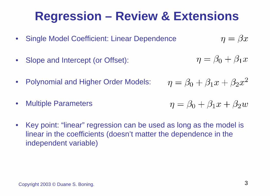
Regression – Review & Extensions
3Copyright 2003 © Duane S. Boning.
• Single Model Coefficient: Linear Dependence
• Slope and Intercept (or Offset):
• Polynomial and Higher Order Models:
• Multiple Parameters
• Key point: “linear” regression can be used as long as the model is linear in the coefficients (doesn’t matter the dependence in theindependent variable)
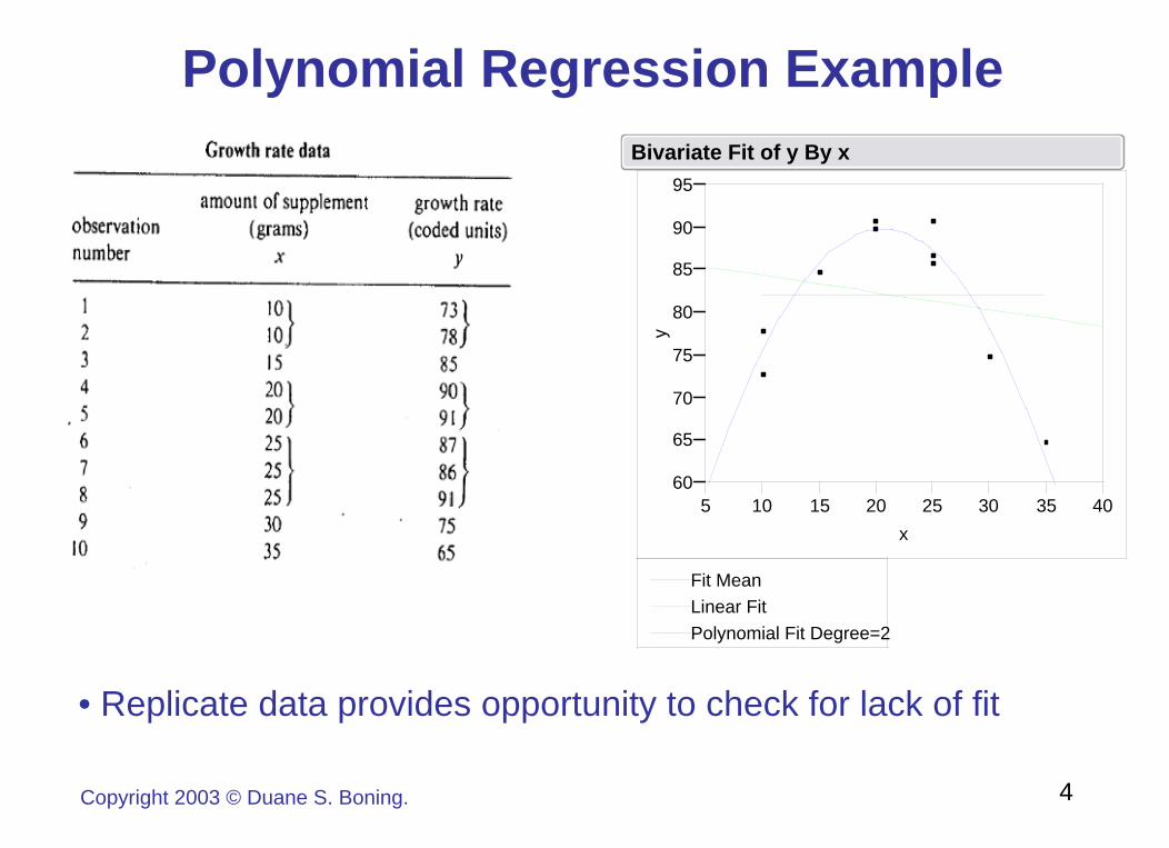
Polynomial Regression Example
• Replicate data provides opportunity to check for lack of fit
60
65
70
75
80
85
90
95
y
5 10 15 20 25 30 35 40x
Fit Mean Linear FitPolynomial Fit Degree=2
Bivariate Fit of y By x
4Copyright 2003 © Duane S. Boning.
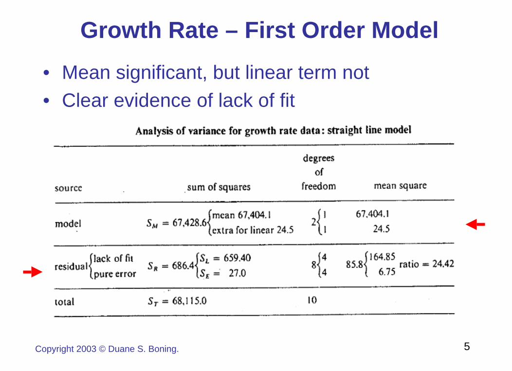
Growth Rate – First Order Model• Mean significant, but linear term not• Clear evidence of lack of fit
5Copyright 2003 © Duane S. Boning.

Growth Rate – Second Order Model
• No evidence of lack of fit• Quadratic term significant
6Copyright 2003 © Duane S. Boning.

Polynomial Regression In Excel
• Create additional input columns for each input• Use “Data Analysis” and “Regression” tool
7Copyright 2003 © Duane S. Boning.
-0.097-0.1582.2E-05-9.9660.013-0.128x^26.5823.9433.1E-059.4310.5585.263x
48.94222.3730.00046.3475.61835.657Intercept
Upper 95%
Lower95%P-valuet Stat
Standard ErrorCoefficients
710.99Total6.45645.1947Residual
6.48E-0551.555332.853665.7062RegressionSignificance FFMSSSdf
ANOVA
10Observations2.541Standard Error0.918Adjusted R Square0.936R Square0.968Multiple R
Regression Statisticsx x 2̂ y10 100 7310 100 7815 225 8520 400 9020 400 9125 625 8725 625 8625 625 9130 900 7535 1225 65

Polynomial Regression
• Generated using JMP
RSquareRSquare Adj
Root Mean Sq ErrorMean of Response
Observations (or Sum Wgts)
0.9364270.9182642.540917
82.110
Summary of Fit
ModelErrorC. Total
Source279
DF665.7061745.19383
710.90000
Sum of Squares332.853
6.456
Mean Square51.5551F Ratio
<.0001Prob > F
Analysis of Variance
Lack Of FitPure ErrorTotal Error
Source347
DF18.19382927.00000045.193829
Sum of Squares6.06466.7500
Mean Square0.8985F Ratio
0.5157Prob > F
0.9620Max RSq
Lack Of Fit
Interceptxx*x
Term35.6574375.2628956-0.127674
Estimate5.6179270.5580220.012811
Std Error6.359.43
-9.97
t Ratio0.0004<.0001<.0001
Prob>|t|Parameter Estimates
xx*x
Source11
Nparm11
DF574.28553641.20451
Sum of Squares88.950299.3151
F Ratio<.0001<.0001
Prob > FEffect Tests
8Copyright 2003 © Duane S. Boning.

Agenda
9Copyright 2003 © Duane S. Boning.
1. Regression• Polynomial regression• Example (using Excel)
2. Time Series Data & Time Series Regression• Autocorrelation – ACF• Example: white noise sequences• Example: autoregressive sequences• Example: moving average• ARIMA modeling and regression
3. Forecasting Examples
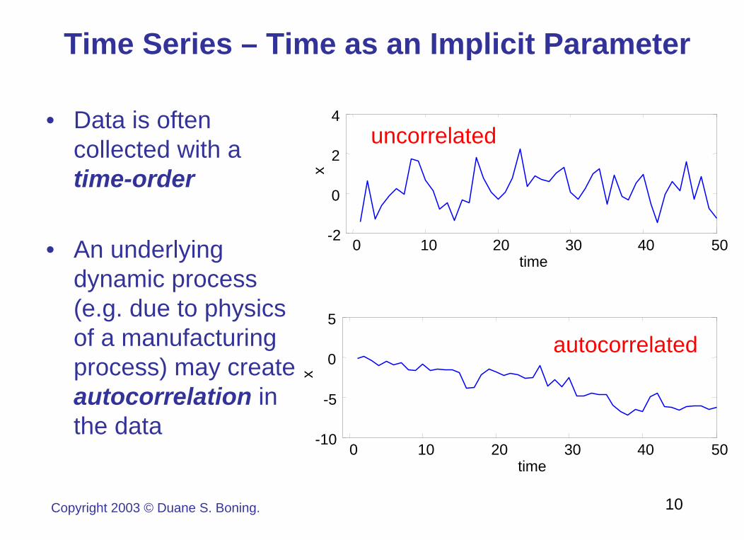
Time Series – Time as an Implicit Parameter
• Data is often collected with a time-order
• An underlying dynamic process (e.g. due to physics of a manufacturing process) may create autocorrelation in the data
0 10 20 30 40 50-10
-5
0
5
time
x
0 10 20 30 40 50-2
0
2
4
time
x
uncorrelated
autocorrelated
10Copyright 2003 © Duane S. Boning.

Intuition: Where Does Autocorrelation Come From?
• Consider a chamber with volume V, and with gas flow in and gas flow out at rate f. We are interested in the concentration x at the output, in relation to a known input concentration w.
11Copyright 2003 © Duane S. Boning.
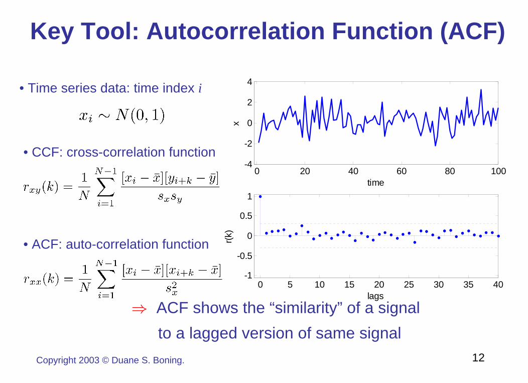
Key Tool: Autocorrelation Function (ACF)
• Time series data: time index i
• CCF: cross-correlation function
• ACF: auto-correlation function
⇒ ACF shows the “similarity” of a signalto a lagged version of same signal
0 20 40 60 80 100-4
-2
0
2
4
time
x
0 5 10 15 20 25 30 35 40-1
-0.5
0
0.5
1
lags
r(k)
12Copyright 2003 © Duane S. Boning.
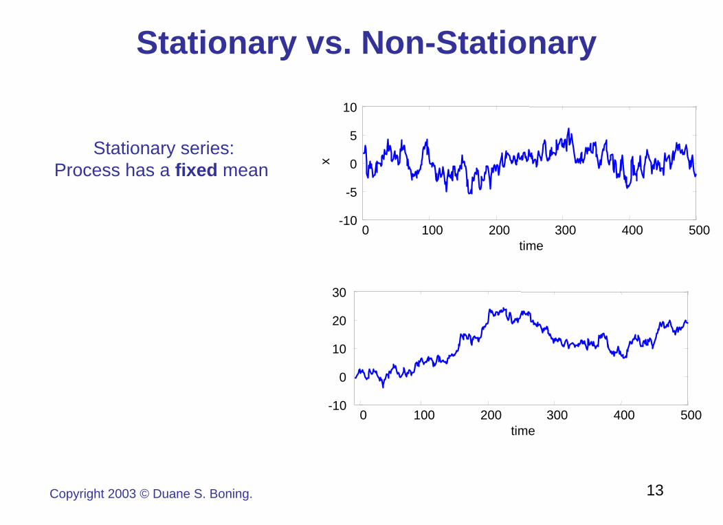
Stationary vs. Non-Stationary
0 100 200 300 400 500-10
-5
0
5
10
time
Stationary series:Process has a fixed mean x
13Copyright 2003 © Duane S. Boning.
0 100 200 300 400 500-10
0
10
20
30
time

White Noise – An Uncorrelated Series
• Data drawn from IID gaussian
• ACF: We also plot the 3σ limits –values within these not significant
• Note that r(0) = 1 always (a signal is always equal to itself with zero lag – perfectly autocorrelated at k = 0)
• Sample mean
• Sample variance
0 50 100 150 200-4
-2
0
2
4
time
x
0 5 10 15 20 25 30 35 40-1
-0.5
0
0.5
1
lags
r(k)
14Copyright 2003 © Duane S. Boning.
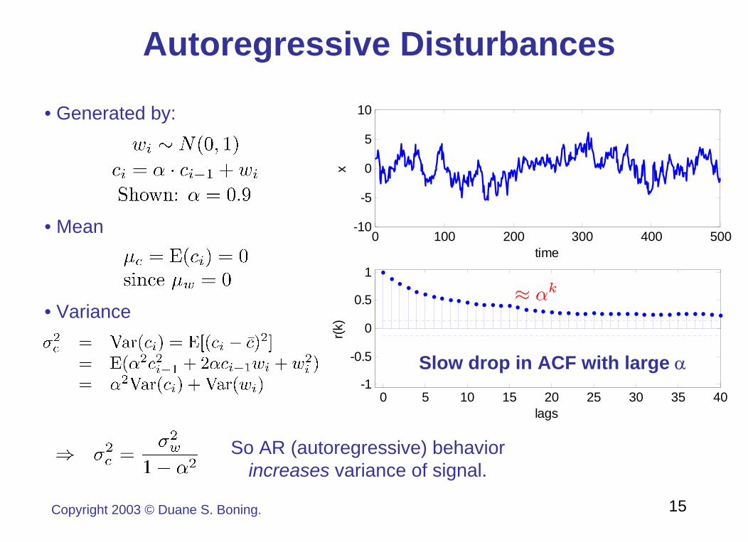
Autoregressive Disturbances
15Copyright 2003 © Duane S. Boning.
0 100 200 300 400 500-10
-5
0
5
10
time
x
0 5 10 15 20 25 30 35 40-1
-0.5
0
0.5
1
lags
r(k)
• Generated by:
• Mean
• Variance
Slow drop in ACF with large α
So AR (autoregressive) behavior increases variance of signal.

Another Autoregressive Series
• Generated by:
16Copyright 2003 © Duane S. Boning.
Slow drop in ACF with large α
0 100 200 300 400 500-10
-5
0
5
10
time
x
0 5 10 15 20 25 30 35 40-1
-0.5
0
0.5
1
lags
r(k)
Slow drop in ACF with large α
But now ACF alternates in sign
• High negative autocorrelation:
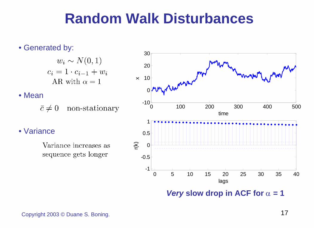
Random Walk Disturbances
• Generated by:
17Copyright 2003 © Duane S. Boning.
0 100 200 300 400 500-10
0
10
20
30
time
x
0 5 10 15 20 25 30 35 40-1
-0.5
0
0.5
1
lags
r(k)
• Mean
• Variance
Very slow drop in ACF for α = 1

Moving Average Sequence
18Copyright 2003 © Duane S. Boning.
0 100 200 300 400 500-4
-2
0
2
4
time
x
0 5 10 15 20 25 30 35 40-1
-0.5
0
0.5
1
lags
r(k)
• Generated by:
• Mean
• Variance
So MA (moving average) behavior also increases variance of signal.
r(1) ≈ β
Jump in ACF at specific lag

ARMA Sequence
19Copyright 2003 © Duane S. Boning.
0 100 200 300 400 500-10
-5
0
5
10
time
x
0 5 10 15 20 25 30 35 40-1
-0.5
0
0.5
1
lags
r(k)
• Generated by:
• Both AR & MA behavior
Slow drop in ACF with large α
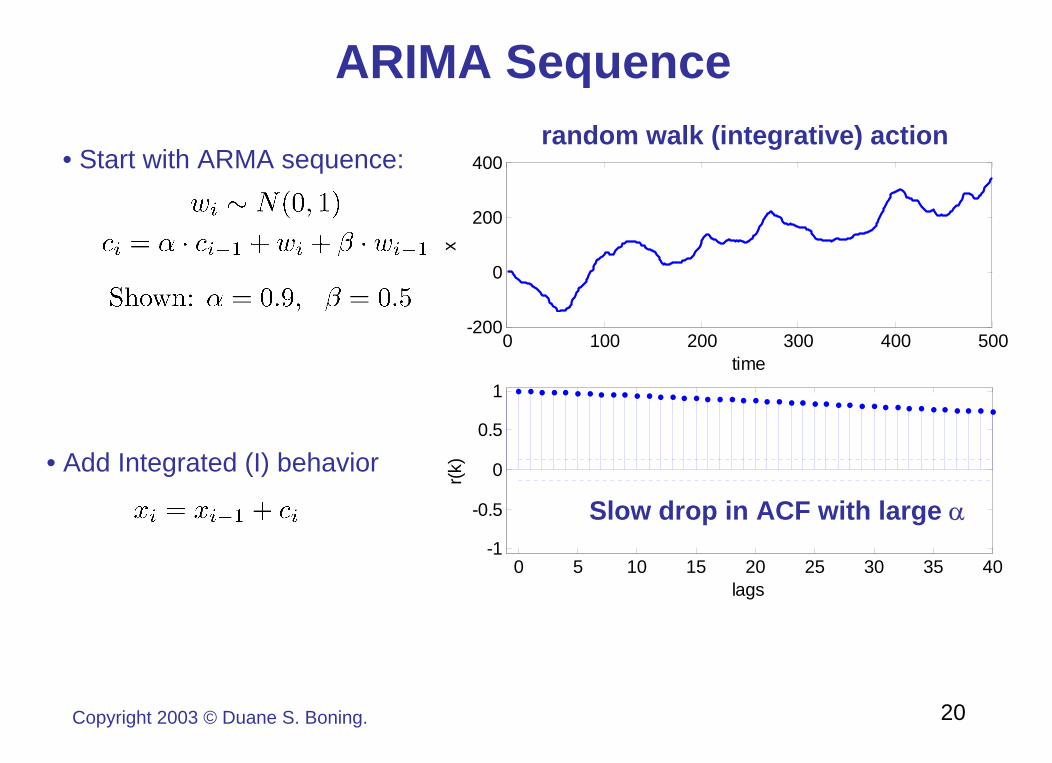
ARIMA Sequence
• Start with ARMA sequence:
0 100 200 300 400 500-200
0
200
400
time
x
0 5 10 15 20 25 30 35 40-1
-0.5
0
0.5
1
lags
r(k)• Add Integrated (I) behavior
Slow drop in ACF with large α
random walk (integrative) action
20Copyright 2003 © Duane S. Boning.
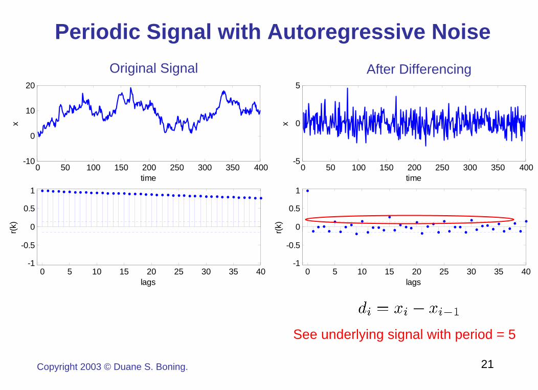
Periodic Signal with Autoregressive Noise
0 50 100 150 200 250 300 350 400-10
0
10
20
time
x
0 5 10 15 20 25 30 35 40-1
-0.5
0
0.5
1
lags
r(k)
Original Signal
0 50 100 150 200 250 300 350 400-5
0
5
time
x0 5 10 15 20 25 30 35 40
-1
-0.5
0
0.5
1
lagsr(k
)
After Differencing
See underlying signal with period = 5
21Copyright 2003 © Duane S. Boning.
Agenda
22Copyright 2003 © Duane S. Boning.
1. Regression• Polynomial regression• Example (using Excel)
2. Time Series Data & Regression• Autocorrelation – ACF• Example: white noise sequences• Example: autoregressive sequences• Example: moving average• ARIMA modeling and regression
3. Forecasting Examples

Cross-Correlation: A Leading Indicator
23Copyright 2003 © Duane S. Boning.
0 100 200 300 400 500-10
-5
0
5
10
time
x
0 100 200 300 400 500-10
-5
0
5
10
time
y
0 5 10 15 20 25 30 35 40-1
-0.5
0
0.5
1
lags
r xy(k
)
• Now we have two series:– An “input” or explanatory
variable x– An “output” variable y
• CCF indicates both AR and lag:

Regression & Time Series Modeling
24Copyright 2003 © Duane S. Boning.
• The ACF or CCF are helpful tools in selecting an appropriate model structure– Autoregressive terms?
• xi = α xi-1
– Lag terms?• yi = γ xi-k
• One can structure data and perform regressions– Estimate model coefficient values, significance, and
confidence intervals– Determine confidence intervals on output– Check residuals

Statistical Modeling Summary
25Copyright 2003 © Duane S. Boning.
1. Statistical Fundamentals• Sampling distributions• Point and interval estimation• Hypothesis testing
2. Regression• ANOVA• Nominal data: modeling of treatment effects (mean differences)• Continuous data: least square regression
3. Time Series Data & Forecasting• Autoregressive, moving average, and integrative behavior• Auto- and Cross-correlation functions• Regression and time-series modeling


