

TEMPORAL AND SPATIAL ANALYSIS OF KILLER WHALE SIGHTINGS
IN THE GALÁPAGOS MARINE RESERVE, ECUADOR
A Thesis
by
KERRI JEAN SMITH
Submitted to the Office of Graduate Studies of Texas A&M University
in partial fulfillment of the requirements for the degree of
MASTER OF SCIENCE
May 2012
Major Subject: Marine Biology

Temporal and Spatial Analysis of Killer Whale Sightings
in the Galápagos Marine Reserve, Ecuador
Copyright 2012 Kerri Jean Smith

TEMPORAL AND SPATIAL ANALYSIS OF KILLER WHALE SIGHTINGS
IN THE GALÁPAGOS MARINE RESERVE, ECUADOR
A Thesis
by
KERRI JEAN SMITH
Submitted to the Office of Graduate Studies of Texas A&M University
in partial fulfillment of the requirements for the degree of
MASTER OF SCIENCE
Approved by:
Co-Chairs of Committee, Douglas C. Biggs
Jane M. Packard Committee Members, William E. Grant Bernd Würsig Intercollegiate Faculty Chair, Gilbert T. Rowe
May 2012
Major Subject: Marine Biology
iii
ABSTRACT
Temporal and Spatial Analysis of Killer Whale Sightings
in the Galápagos Marine Reserve, Ecuador. (May 2012)
Kerri Jean Smith, B.S., Texas A&M University at Galveston
Co-Chairs of Advisory Committee: Dr. Douglas C. Biggs Dr. Jane M. Packard
A study was conducted using data compiled from two sources to test the
hypothesis that killer whales display seasonal variability in their occurrence in the
Galápagos Marine Reserve (GMR), Ecuador. Three questions arise from this hypothesis:
1) do killer whale sightings display temporal variability; 2) are sightings spatially
associated with resources; and 3) if sightings are spatially associated with resources,
does the spatial association change temporally? I combined and evaluated two sets of
GMR killer whale sighting data (n=154) spanning a twenty-year time frame collected
via opportunistic sightings by an observer network and shipboard line-transect surveys.
I tested for a (a) correlation between the total annual sightings and bi-annual seasonality
(upwelling versus non-upwelling); (b) correlation between the total annual sightings and
the Multivariate El Niño Southern Oscillation Index (MEI); (c) correlation between
sightings, the MEI, and seasonality; (d) spatial association between sightings and
resources; and (e) spatial change in sightings with seasonality. Sightings were roughly
equally distributed between non-upwelling (56%) and upwelling seasons

iv
(July-December). No direct correlation was found between sightings and the MEI.
Sightings occurred more often than expected by chance during the peak upwelling
months of August-November when the MEI was within one standard deviation of the
average (binomial z=2.91, p<0.05). Sightings were spatially associated with areas of
high chlorophyll a values (binomial z=4.46, p<0.05), pinniped rookeries (binomial
z=6.03, p<0.05), and areas with high combined resource value (binomial z=5.36,
p<0.05). The spatial distribution of sightings did not shift with seasonality, with the
exception that sightings occurred less often than expected in areas of low combined
resource value during the upwelling period (binomial z=-3.17, p<0.05). Though
variability in observer effort should be considered when evaluating these data, these
results do not suggest a strong pattern of seasonal occupancy or that killer whales are
responsive to El Niño Southern Oscillation events. Further research is needed to
determine if killer whales in the GMR comprise a single resident population, multiple
resident and transient populations, or if killer whales observed in the GMR are part of a
population inhabiting the eastern tropical Pacific region, which visit the area at various
times.

v
DEDICATION
I dedicate this work to my family; without your love, support and
encouragement this would not have been possible. Thank you for always
being patient as I excitedly rambled about my latest idea, acting as a
sounding board at all hours, and helping me to laugh at myself.

vi
ACKNOWLEDGEMENTS
This thesis is the culmination of the work of numerous individuals; many of
whom I will never be able to thank, and all of whom I will never be able to thank
enough. To my major advisors, Drs. Douglas Biggs and Jane Packard, thank you for
your unending patience, support, guidance, and advice. Dr. Biggs introduced me to the
wonder that is the Galápagos Islands, provided me with the tools to better understand
oceanographic processes, and helped me hone my critical thinking skills. Dr. Packard,
provided a warm, dynamic laboratory environment in which my ideas could grow and
flourish. To my committee members, Drs. Bernd Würsig and William Grant, thank you
for helping me to shape my ideas and ask the right questions, and for your advice and
guidance on this manuscript. Dr. Christopher Marshall, thank you for all of the advice
over the years, for providing me with research opportunities as an undergraduate student,
and for being available when I needed an ear to bend. To the Department of
Oceanography, College of Geosciences, and the Marine Biology Interdisciplinary
Program, thank you for providing the funds for travel and research in Ecuador. The
Departments of Oceanography and Biology supplied funding in the form of teaching
assistantships and the Department of Wildlife and Fisheries provided funding in the form
of a research assistantship.
A great thank you is due to Godfrey Merlen, without whom this work would not
be possible. His dedication to understanding and protecting the Galápagos Island
ecosystem will forever be an inspiration to me and many more. His tireless efforts to
gather historical records of killer whale observations and work to build a network of

vii
citizen observers within the Galápagos Islands provided a huge chunk of the killer whale
data analyzed in this project. Dr. Daniel Palacios, despite not having any idea who I was,
answered my e-mails kindly, thoughtfully, and knowledgably. His work on cetaceans
and ecosystem dynamics in the Galápagos Islands helped to lay the groundwork for this
project, and he provided the additional killer whale data analyzed in this manuscript. Dr.
Juan Jose Alava contributed his data on Galápagos sea lions to this project, in addition to
freely sharing his ideas and thoughts. His kind and encouraging words were often just
what I needed to help me push through a particularly grueling bit of analyses. I will
never be able to thank these three enough for their generous support and wonderful
guidance.
To the hundreds of individuals who helped to collect the data used in this
analysis, thank you. I may never know your name, or be able to shake your hand, but
you were an integral part of this project. Your willingness to share your photos,
observations, and knowledge of killer whales in the Galápagos Islands made this
research possible.
Julia O’Hern took me under her wing and taught me about being a field biologist,
shared ideas and provided invaluable guidance and camaraderie. Olivia Lee, Shannon
Finerty, Lacy Madsen, and Tiffany Walker, I can’t thank you enough for all of your
support in all aspects of my life and this project.
And last but not least, thank you to my family, who stuck by me through the ups
and downs of this project and still answered the phone even though they knew it was me

viii
calling. While there are many people who deserve my thanks and who contributed to this
work, without your strong support this venture would not have been successful.

ix
NOMENCLATURE
CZCS Coastal Zone Color Scanner
ENSO El Niño Southern Oscillation
ETP Eastern Tropical Pacific
GMR Galápagos Marine Reserve
MEI Multivariate ENSO Index
MODIS Moderate Resolution Imaging Spectroradiometer
MPA Marine Protected Area
NOAA National Oceanographic and Atmospheric Association
SeaWiFS Sea-viewing Wide Field-of-view Sensor

x
TABLE OF CONTENTS
Page
ABSTRACT .............................................................................................................. iii
DEDICATION .......................................................................................................... v
ACKNOWLEDGEMENTS ...................................................................................... vi
NOMENCLATURE .................................................................................................. ix
TABLE OF CONTENTS .......................................................................................... x
LIST OF FIGURES ................................................................................................... xii
LIST OF TABLES .................................................................................................... xiv
CHAPTER
I INTRODUCTION ................................................................................ 1 II TEMPORAL ANALYSIS .................................................................... 4
Introduction .................................................................................... 4 Methods .......................................................................................... 7 Results ............................................................................................ 12 Discussion ...................................................................................... 18
III SPATIAL ANALYSIS ........................................................................ 21
Introduction .................................................................................... 21 Methods .......................................................................................... 25 Results ............................................................................................ 33 Discussion ...................................................................................... 39
IV TEMPORAL AND SPATIAL INTERACTION ................................. 42
Introduction .................................................................................... 42 Methods .......................................................................................... 45 Results ............................................................................................ 47 Discussion ...................................................................................... 54

xi
CHAPTER Page V SUMMARY AND CONCLUSIONS ............................................................ 56 Summary ........................................................................................ 56 Conclusions .................................................................................... 58 Recommendations for future research ............................................ 60
REFERENCES .......................................................................................................... 61
VITA ......................................................................................................................... 73
xii
LIST OF FIGURES
FIGURE Page
1 The study area: the Galápagos Marine Reserve, shaded, and surrounding waters. ............................................................................................ 9
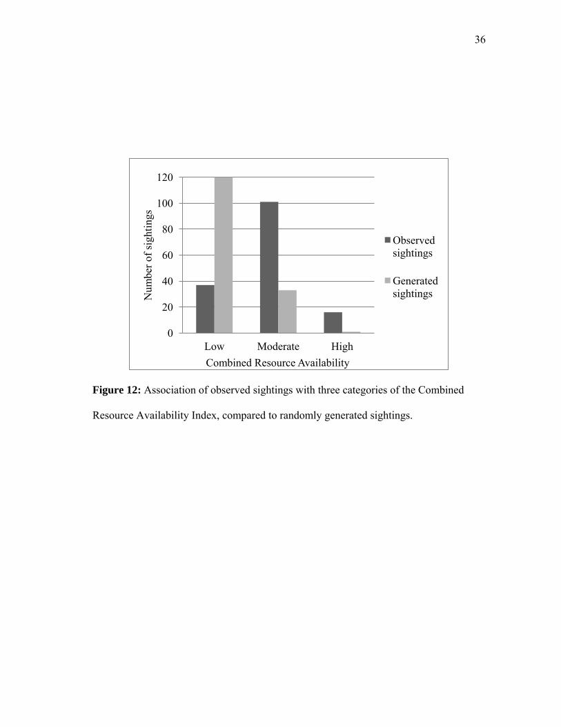
2 Monthly distribution of killer whale sightings for the study period. ......... 13 3 Seasonal distribution of killer whale sightings for the study period .......... 14 4 Number of killer whale sightings and the Multivariate El Niño Southern Oscillation Index for each year ................................................... 15 5 Multivariate El Niño Southern Oscillation Index for each year and number of killer whale sightings the following year .................................. 16 6 Spatial map of killer whale sightings (1976-1997), combining results of opportunistic and systematic surveys ..................................................... 28 7 Spatial map of randomly generated data points used for comparison of available and observed habitat conditions associated with killer whale sightings ........................................................................................... 29 8 Composite chlorophyll a map generated from MODIS satellite data for the period January 2003 – December 2010 .......................................... 30 9 Sea lion rookery and haul out locations in the Galápagos Marine Reserve ....................................................................................................... 31 10 Association of observed sightings with three categories of the Productivity Index, compared to randomly generated sightings ................ 34 11 Association of observed sightings with three categories of the Vulnerable Prey Index, compared to randomly generated sightings.......... 35 12 Association of observed sightings with three categories of the Combined Resource Availability Index, compared to randomly generated sightings ..................................................................................... 36 13 Killer whale sightings mapped with two areas of higher spatial use identified ..................................................................................................... 38

xiii
14 Non-upwelling versus upwelling sightings per level of the Productivity Index ...................................................................................... 48 15 Non-upwelling versus upwelling sightings per level of the Vulnerable Prey Index ................................................................................ 49 16 Non-upwelling versus upwelling sightings per level of the Combined Resource Availability Index. ..................................................................... 50
17 Spatial distribution of sightings during the non-upwelling season ............ 52 18 Spatial distribution of sightings during the upwelling season .................... 53

xiv
LIST OF TABLES
TABLE Page 1 A summary of the number of sightings and the Multivariate El Niño Southern Oscillation Index condition each year of the study period. ........ 10 2 A summary of the Multivariate El Niño Southern Oscillation Index value for each El Niño Southern Oscillation condition .............................. 11 3 Test results for the strength of association between sightings and upwelling season ........................................................................................ 17 4 Indices for Productivity, Vulnerable Prey, and Combined Resource Availability ................................................................................................. 32 5 Summary of spatial analysis results ........................................................... 37
6 Summary of temporal-spatial analysis results ............................................ 51
1
CHAPTER I
INTRODUCTION
In the Galápagos Marine Reserve and surrounding waters (GMR) killer whales
(Orcinus orca) remain an enigmatic species, with most aspects of their biology unknown
(Merlen, 1999). Line-transect surveys of the eastern tropical Pacific (ETP) suggest an
estimated population of 8,500 killer whales (Wade and Gerrodette, 1993), but it is
unknown how many of these animals might utilize the GMR. Merlen (1999) reports
sightings of killer whales within the GMR throughout the year, but the information gap
leaves an open question: does a resident population exist or is the area used only for
transit or as a stop-over point during long-range movements? The purpose of this study
is to examine multi-year killer whale sighting data from the GMR to test the residency
hypothesis and provide direction for future research efforts.
The GMR is subject to both annual seasonal changes and multi-decadal cyclic El
Niño Southern Oscillation (ENSO) events (Sweet et al, 2007), both of which may impact
foraging resources available for killer whales (Ballance et al, 2006). El Niño events
bring warm air to the region, which suppresses upwelling and decreases southeast trade
wind strength and oceanic mixing, while La Niña events amplify mixing and upwelling
with cool air and an increase in southeast trade wind strength (Palacios, 2003). I
hypothesize that if resource availability and abundance changes on a temporal scale,
____________ This thesis follows the style of Latin American Journal of Aquatic Mammals.

2
killer whales may visit the GMR at various times throughout the year to take advantage
of these resource pulses. In Chapter II, I test for a relationship between annual killer
whale sightings and environmental temporal variability. If killer whale presence is
seasonal, rather than permanent, then I expect to find months with little to no killer
whale sightings and a correlation between the strength of an ENSO event and the
number of killer whale sightings. To address this hypothesis, I test for (a) a correlation
between the total annual killer whale sightings and annual seasons; (b) a correlation
between the total annual sightings and the Multivariate ENSO Index (MEI); and (c) an
association between sightings, the MEI, and seasonal upwelling.
Observations of foraging killer whales in the GMR provide insight into some of
the resources they may be utilizing. Killer whales have been observed within areas of
high chlorophyll a productivity, where they are known to harass and possibly predate
cetacean assemblages, and have been observed feeding on manta rays, ocean sunfish, sea
turtles, and possibly hammerhead sharks (Palacios, 2003; Sorisio, 2006; Alava and
Merlen, 2009; Merlen, personal communication, 2010). They have also been observed
hunting and predating Galápagos sea lions throughout the archipelago (Merlen, 1999;
Merlen, personal communication, 2010; Alava, personal communication, 2011). I
hypothesize that if killer whales are feeding in areas of high productivity and on sea
lions, then killer whale observations may be more spatially associated with regions
where these resources are abundant than in areas where they are less abundant. In
Chapter III, I test for a relationship between the spatial distribution of killer whale
sightings, high chlorophyll a productivity, and sea lion rookeries.
3
Chlorophyll a productivity in the GMR is highly dependent upon temporal
variability, which may in turn have bottom-up influences on the abundance of important
prey resources for killer whales (Trillmich and Limberger, 1985; Smith and Whitehead,
1993; Ballance et al., 2006; Hunt 2006; Karnauskas et al., 2010). I hypothesize that if
killer whales are found to be spatially associated with chlorophyll a and sea lion
rookeries, and they are present in the GMR for most of the year, then they may alter their
spatial distribution in response to temporal variability of these resources. In Chapter IV,
I address this hypothesis by testing for a shift in killer whale sighting spatial distribution
with respect to seasonality.
The ultimate goal of this work is to publish baseline values on killer whale
sighting temporal and spatial distribution in the Galápagos Marine Reserve. To
accomplish this goal I will aim to publish three chapters from this thesis. Chapters II and
III will answer basic questions about the temporal and spatial distribution of killer
whales sightings within the GMR, and will be submitted for publication to the Latin
American Journal of Aquatic Mammals. Building on the results of the tests conducted in
Chapters II and III, Chapter IV combines and expands upon the temporal and spatial
tests to gain a further understanding of how killer whale sightings are spatially
distributed within the GMR in response to temporal fluctuation. Chapter IV will be
submitted for publication in PLoS One. Both the Latin American Journal of Aquatic
Mammals and PLoS One are free access journals that will make the results of this study
readily and freely available to international scientists. In Chapter V, a summary of my
thesis research and some recommendations for future research are provided.
4
CHAPTER II
TEMPORAL ANALYSIS
Introduction
Killer whale sightings in the Galápagos Marine Reserve and surrounding waters
(GMR) have been reported since 1948, yet little is known about their residency in this
region (Merlin, 1999). Analyzing opportunistically collected data, Merlen (1999)
reported sightings of killer whales within the GMR throughout the year. Wade and
Gerrodette (1993) estimated a population of 8,500 killer whales in the Eastern Tropical
Pacific (ETP), but it is unknown if killer whales observed in the GMR are part of this
population. This information gap leaves an open question: does a resident population
exist or is the area used as stop-over point during long-range movements?
Killer whale populations are known to make short- and long-range movements of
various distances, from hundreds to thousands of kilometers (Hauser et al, 2007; Krahn,
et al, 2007; Andrews et al, 2008; Dahlheim, et al, 2008; Foote et al, 2010; Matthews et
al, 2011). A recent study by Durban and Pitman (2011) indicates that at least one
ecotype undertakes long-distance migrations. In other locations killer whales are known
to move between resources on a seasonal basis and take advantage of increased prey
availability during resource pulses (Foote et al, 2010; Reisinger et al, 2011).
Seasonal resource abundance varies greatly between southern hemisphere
ecosystems, with strong seasonal shifts occurring near the pole and weaker shifts
occurring near the equator. In the frigid Antarctica and sub-arctic waters, where
5
nutrients are plentiful, the sun acts as the driving force in productivity (Sewell and Jury,
2011; Teschke et al, 2011). The extreme shift from a 24 hour photo-period to a 24-hour
sun-absent period between seasons results in short-growing high-amplitude
phytoplankton and zooplankton blooms in the austral spring and summer (Sewell and
Jury, 2011; Teschke et al, 2011). During the austral autumn the resting stages for these
blooms lie dormant and primary productivity drastically decreases (Sewell and Jury,
2011; Teschke et al, 2011). In the tropics and sub-tropics nutrients are scarce and the
photic period is long and consistent throughout the year, resulting in long-growing low-
amplitude blooms (Racault et al, 2012). In pelagic ecosystems productivity can be very
low due to low nutrient levels, whereas tropical coastal regions are more productive due
to upwelling and increased nutrient levels (Racault et al, 2012). The GMR is unusual
among tropical pelagic regions in that it has higher than average primary productivity
(Palacios, 2003; Schaeffer et al., 2008) which may make it an ideal foraging resource for
killer whales undertaking long-distance movements or migrations, or when seasonal
resource abundance decreases in other areas.
Strong El Niño events suppress upwelling, a driving force behind the high
primary productivity of the GMR (Sweet et al., 2007; Schaeffer et al., 2008), which may
in turn decrease the amount of resources available for killer whales. Strong El Niños
have been shown to have a lasting effect on the community structure in the GMR, as
evidenced by the 1982-1983 El Niño event that resulted in 100% mortality for
Galápagos sea lion pups born in 1982 and an 89% reduction in the number of pups born
the following year (Alava and Salazar, 2006). Killer whales may respond to these
6
fluctuations in potential prey availability by leaving the GMR following these events.
Changes to the cetacean community structure as a result of ENSO events have been
reported in several locations (e.g. Monterey Bay, California; the Gulf of California;
Magdalena Bay, Mexico; Bahia de la Paz, Mexico) and may affect the habitat use and
community structure of cetaceans in the GMR (Flores-Ramirez et al, 1996; Gardner and
Chavez-Rosales, 2000; Benson et al, 2002; Salvadeo et al, 2011). If resource availability
and abundance changes on a temporal scale, killer whales may visit the GMR at various
times throughout the year to take advantage of these resource pulses and vacate the
GMR when strong ENSO events severely depress resource availability.
The aim of this chapter is to provide new information about the seasonal and
inter-annual occurrence of killer whale sightings within the GMR with regard to annual
seasonal changes and cyclic El Niño Southern Oscillation events. To achieve this, I
analyzed data involving temporal distribution collected via opportunistic sightings by an
observer network and shipboard line-transect surveys over a 20 year time frame.

7
Methods
Data collection and reduction
Killer whale sightings analyzed in this study were collected between the
geographic coordinates 94°W and 87°W, 3°N and 3°S (Figure 1). Sightings collected via
the observer network were collected opportunistically and with variable effort between
1948 and 1997 by Galápagos National Park tour guides, boat captains, scientists, and
film makers (Merlen, 1999). Sightings collected via line transect were collected between
1976 and 2000 on the Ocean Alliance vessels Odyssey and Siben and NOAA South West
Fisheries Science Center research and tuna vessels (Palacios, personal communication
2010). A total of 175 sightings were available for analysis, but only data collected
between 1976 and 1997 were analyzed (n = 154). For years 1977 and 1984 no data were
available and thus were treated as missing data. This 22 year time frame was chosen
because both collection methods were being employed and no more than one year passed
without killer whale sightings.
Data analysis
To assess whether any changes in the seasonal or interannual occurrence of killer
whales were related to environmental variability, two variables were considered: (1)
seasonal upwelling and productivity; (2) the Multivariate ENSO Index (MEI) available
from the NOAA Earth System Research Laboratory (ESRL, 2011). I tested for (a) a
relationship between annual sighting abundance and seasonal upwelling (b) a correlation
between the total annual killer whale sightings and the MEI, (c) a correlation between

8
the total annual killer whale sightings and the MEI of the previous year, and (d) an
association between killer whale sightings, the ENSO index, and seasonal upwelling.
Upwelling was initially defined as a six month period of increased chlorophyll a
which consisted of months July – December. Within these six months, July and
December may act as transitional months that bound the “peak” upwelling period lasting
three to four months and occurring August – November (Sweet et al., 2007; Schaeffer et
al., 2008). After excluding the transitional months of July and December, I used a
binomial z test (Bakeman and Gottman, 1986) to measure the association between killer
whale sightings, the ENSO index, and seasonal upwelling with two three-month
variations of this peak, August – October and September – November, and a four month
peak of August – November.
I assigned a MEI value to each year of analysis according to the NOAA MEI
bimonthly values (Table 1). Each year was classified as either “normal,” “El Niño,” or
“La Niña.” Normal conditions were defined as less than one standard deviation from the
norm (0); El Niño conditions were defined as at least one positive standard deviation
from the norm (1, 2, or 3); La Niña conditions were defined as at least one negative
standard deviation from the norm (-1, -2, or -3) (Table 2). If at least one month of the
year exhibited a non-normal condition, the year was classified as non-normal. If a year
exhibited both El Niño and La Niña conditions, the year was classified according to the
more prominent condition, determined by the total number of months each condition was
present. The strength of the deviation for the year was assigned according to the
strongest deviation present that year.

9
Figure 1: The study area: the Galápagos Marine Reserve, shaded, and surrounding
waters. Map created with SEATURTLE.org/Maptool.

10
Table 1: A summary of the number of sightings and the Multivariate El Niño Southern
Oscillation Index condition each year of the study period.
YEAR NUMBER OF
SIGHTINGS
MULTIVARIATE EL NIÑO
SOUTHERN OSCLLATION EVENT INDEX
VALUE 1976 5 -1 1978 8 0 1979 1 1 1980 8 0 1981 15 0 1982 7 2 1983 3 3 1985 3 0 1986 5 1 1987 2 2 1988 6 -1 1989 10 -1 1990 1 0 1991 5 1 1992 5 2 1993 24 1 1994 13 1 1995 12 1 1996 18 0 1997 3 2

11
Table 2: A summary of the Multivariate El Niño Southern Oscillation Index value for
each El Niño Southern Oscillation condition.
EL NIÑO SOUTHERN OSCILLATION
CONDITION
MULTIVARIATE EL NIÑO SOUTHERN
OSCILLATION EVENT INDEX VALUE(S)
Normal 0 El Niño 1, 2, or 3 La Niña -1, -2 , or -3
12
Results
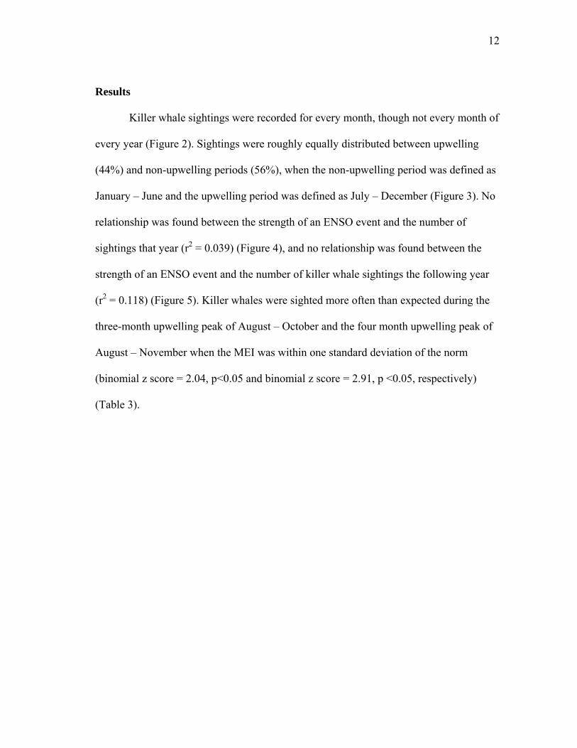
Killer whale sightings were recorded for every month, though not every month of
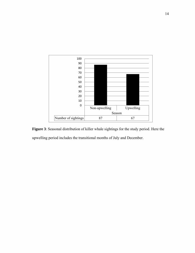
every year (Figure 2). Sightings were roughly equally distributed between upwelling
(44%) and non-upwelling periods (56%), when the non-upwelling period was defined as
January – June and the upwelling period was defined as July – December (Figure 3). No
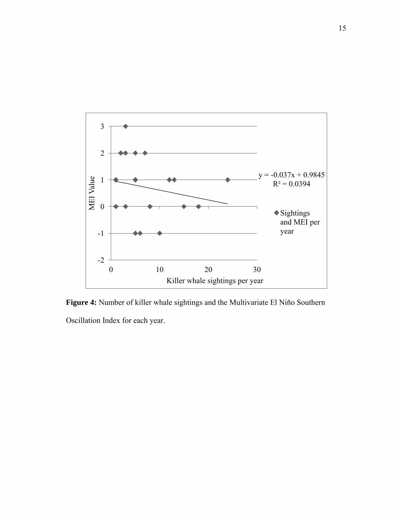
relationship was found between the strength of an ENSO event and the number of
sightings that year (r2 = 0.039) (Figure 4), and no relationship was found between the
strength of an ENSO event and the number of killer whale sightings the following year
(r2 = 0.118) (Figure 5). Killer whales were sighted more often than expected during the
three-month upwelling peak of August – October and the four month upwelling peak of
August – November when the MEI was within one standard deviation of the norm
(binomial z score = 2.04, p<0.05 and binomial z score = 2.91, p <0.05, respectively)
(Table 3).

13
Figure 2: Monthly distribution of killer whale sightings for the study period.
29
11 8
18
7
14
6
24
6 8
11 12
Jan Feb Mar Apr May Jun Jul Aug Sep Oct Nov Dec
14
Figure 3: Seasonal distribution of killer whale sightings for the study period. Here the
upwelling period includes the transitional months of July and December.
Non-upwelling Upwelling Season
Number of sightings 87 67
0
10
20
30
40
50
60
70
80
90
100
15
Figure 4: Number of killer whale sightings and the Multivariate El Niño Southern
Oscillation Index for each year.
y = -0.037x + 0.9845 R² = 0.0394
-2
-1
0
1
2
3
0 10 20 30
MEI
Val
ue
Killer whale sightings per year
Sightings and MEI per year

16
Figure 5: Multivariate El Niño Southern Oscillation Index for each year and number of
killer whale sightings the following year.
y = 0.0597x - 0.0099 R² = 0.1189
-2
-1
0
1
2
3
0 5 10 15 20 25
MEI
Val
ue
Number of sightings following year
Sightings and MEI per year

17
Table 3: Test results for the strength of association between sightings and upwelling
season, based on three definitions of the upwelling peak when the Multivariate El Niño
Southern Oscillation Index was within one standard deviation of the average.
UPWELLING PEAK BINOMIAL Z SCORE
P-VALUE
August - October 2.04 < 0.05
September - November 0.26 > 0.05
August - November 2.91 < 0.05

18
Discussion
This study represents the first time that multiple reports of killer whale sightings
in the GMR have been synthesized and analyzed for temporal patterns. With the caveat
that the data collection efforts were not consistent across the collection period, these
results provide new insights into the temporal patterns of killer whale sightings in the
GMR.
These results support the hypothesis of a continuous killer whale presence in the
GMR from month to month and most years. The two years (1977 and 1984) with
missing data could be a result of: a) no line-transect surveys conducted those years, b) no
observations recorded or reported by opportunistic observers, or c) low killer whale
presence due to fluctuating environmental factors. Though I found no association
between the strength of an ENSO event and the number of killer whales observed in the
following year, no killer whales were observed in 1984, directly following the only El
Niño event with a standard deviation of 3 within the study period. Trillmich and
Limberger (1985) and Alava and Salazar (2006) report that extreme El Niño events, such
as the very strong one that occurred in 1983, have devastating effects on pinniped
populations within the GMR, Vargas et al. (2007) demonstrated that the 1983 El Niño
event had a catastrophic effect on the population of Galápagos penguins (Spheniscus
mendicus), and Edgar et al (2010) suggests that the GMR underwent severe
transformation at the autotrophic level following the 1983 El Niño. Strong El Niño
events suppress upwelling, a driving force behind the high productivity of the GMR
19
(Sweet et al., 2007; Schaeffer et al., 2008), which may in turn decrease the amount of
potential prey resources available for killer whales.
That killer whales were sighted more often than expected during the previously
defined peak upwelling periods (August – October, and August – November) when the
MEI was normal, may be an indicator of the number of observers present rather than a
greater abundance of killer whales. If resources are more abundant during these times
there may be more people on the water to take advantage of those resources, and thus
more reports of killer whales. This is not to say that killer whales are not more abundant
during these periods, but that the interpretation of these results needs to take that
possibility into consideration.
Further research needs to be conducted to determine if the same individuals are
observed repeatedly or if multiple groups of killer whales are using the GMR throughout
the year. Photo identification projects have proven successful for identifying individual
killer whales, social groups and residency in other populations, such as Alaska, the
Eastern Tropical Pacific, and along the Northwest Pacific coast of North America (e. g.
Dahlheim, 1997; Olson and Gerrodette, 2008, Durban et al, 2010). A similar photo
identification project in the GMR could prove very valuable in identifying residency
patterns of killer whales. Durban and Pitman (2011) and Matthews et al. (2011) both
report the success of placing satellite tags on killer whales to gain valuable new insight
into their long distance movements. Placing satellite tags on killer whales in the GMR
could be a valuable tool to learn more about their movement and habitat use, and if
GMR killer whales are migrants from other regions.

20
These results do not suggest a strong pattern of seasonal occupancy and provide
sufficient evidence to reject the hypothesis that killer whales observed in the GMR are
present during specific times to take advantage of resource pulses. They do support an
alternative pattern, such as a single resident population, multiple resident and transient
populations, or that killer whales observed in the GMR are part of a population
inhabiting the eastern tropical Pacific region that visit the GMR throughout the year. To
better understand what role, if any, seasonality and ENSO events have on killer whales
in the GMR additional research needs to be conducted on the spatial distribution of
sightings. Merlen (1999) and Palacios (2003) report that GMR killer whales have been
observed predating sea lions, possibly predating cetaceans, and foraging in areas of high
chlorophyll a productivity. As Chapter III will show, statistical analysis of the spatial
distribution of GMR killer whale sightings may help to identify key habitats and
resources.

21
CHAPTER III
SPATIAL ANALYSIS
Introduction
Though some coastal killer whale populations have been extensively studied and
are well understood (i. e. the resident ecotype of northwest North America), only a
handful of island killer whale populations have been studied. In the southern hemisphere
killer whales have been studied around the Prince Edward Islands (PEI) and the Crozet
Islands. At the PEI killer whales are observed feeding on fur seals (Arctocephalus
tropicalis), elephant seals (Mirounga leonine) and several species of penguins,
(Reisinger et al, 2011). PEI killer whales are present all year with peaks in abundance
occurring twice a year, coinciding with an increase in the abundance of penguins and
pinnipeds (Reisinger et al, 2011). At the Crozet Islands, located at similar latitude as the
PEI, killer whales are observed feeding on fish, penguins, and elephant seals using
multiple different foraging tactics. These include patrolling the mouth of rivers where
pinniped pups swim, in areas with dense algae cover along penguin colonies, and
occasionally predating large cetaceans (Guinet, 1992; Guinet et al, 2000). Like the killer
whales at the PEIs, these killer whales are also present all year with occasional
abundance peaks that coincide with an increase in prey abundance (Guinet, 1992; Guinet
et al, 2000).
In the northern hemisphere, killer whales have been studied in the Aleutian
Islands and Hawaii. Killer whales observed in the Aleutian Islands are part of the

22
transient ecotype known to predate a wide variety of marine mammals, including several
species of pinnipeds, river and sea otters, and other cetaceans (Dahlheim et al, 2008;
Durban et al, 2010; Matkin et al, 2007). These killer whales are known to travel long
distances in order to take advantage of increases in resource abundance and distribution;
a recent study by Barrett-Lennard et al (2011) demonstrated that 150+ killer whale
annually aggregate around Unimak Island to predate migrating gray whales, often
feeding for several days on the submerged carcasses of their prey. In the Hawaiian
Islands, a tropical island ecosystem similar the Galápagos Islands, killer whales are
infrequently observed yet are known to be present in the region at least nine months of
the year (Baird et al, 2006). They are thought to be generalist predators and have been
observed predating both cephalopods and humpback whales (Baird et al, 2006).
Killer whales are observed in the Galápagos Marine Reserve and surrounding
waters throughout the year, though very little is known about how they are distributed
throughout the region or their habitat use (Merlen, 1999; Chapter II). In the GMR, killer
whales have been observed near every major island and have been recorded foraging on
a diverse array of prey, including cetaceans, sea lions, sharks and rays, fish, and sea
turtles (Merlen, 1999; Palacios, 2003; Merlen and Alava, 2009). Merlen (1999) reports
that of 135 sightings, 45 (40%) occurred near sea lion rookeries, and Palacios (2003)
found that killer whales attacked cetaceans along upwelling zones where levels of
chlorophyll a are high. Despite these observations and reports, it is still unknown if
sightings are spatially associated with these resources and how killer whales are moving
throughout the region.
23
Seasonal upwelling in the GMR is the driving force behind increased primary
productivity and standing crops of chlorophyll a, which in turn are responsible for the
high abundance and biodiversity of resources in the region (Sweet et al, 2007; Schaeffer
et al, 2008). Because primary productivity provides bottom-up forcing for the GMR
ecosystem, increased standing crops of chlorophyll a should lead to increased standing
crops of the mid-trophic level resources that killer whales predate (e. g. fish, squid, and
baleen whales) (Hunt 2006; Alava, 2009). While distribution and abundance data for
many of these mid-trophic level resources are scarce, remotely sensed chlorophyll a data
are readily available and can serve as a proxy to indicate areas where mid-trophic levels
resources may be located.
Pinnipeds are highly mobile upper trophic level predators that constitute an
important role in the diet of several killer whale populations (e.g.: the transient ecotypes
of western North America; Crozet Islands; Marion Islands, and Punta Norte, Argentina)
(Lopez and Lopez, 1985; Guinet, 1992; Hoelzel, 1991; Ford et al, 1998; and Pistorius et
al, 2002). In the GMR there are two resident pinniped species, the Galápagos sea lion
and the Galápagos fur seal, both of which killer whales have been observed predating.
However, only one known attack has occurred on fur seals, and sea lions are more
populous and widely distributed. The majority of sea lion rookeries are found near the
center of the archipelago but they frequently travel to other islands or are encountered at
sea, while fur seal colonies are predominantly located on Isabela and Fernandina Islands
along the outer western edge of the archipelago, and they rarely travel to other islands
(Jeglinski et al, 2011; personal observation). Jeglinski et al (2011) found that fur seals
24
and sea lions overlap in their distribution along the western islands and fur seals and
juvenile sea lions both feed primarily at night, while adult sea lions feed both night and
day. Merlen (2000) also found that fur seals were more active acoustically at night than
during the day. Due to the size discrepancy in adult sea lions and fur seals/juvenile sea
lions, nocturnal foraging may be an anti-predator strategy by these smaller animals to
avoid predation. However, Jeglinski (personal communication 2011) found that killer
whale presence elicited no visual response from fur seals who were in the water when
killer whales passed by, suggesting that fur seals may not be frequently predated by
killer whales.
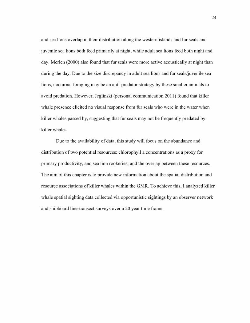
Due to the availability of data, this study will focus on the abundance and
distribution of two potential resources: chlorophyll a concentrations as a proxy for
primary productivity, and sea lion rookeries; and the overlap between these resources.
The aim of this chapter is to provide new information about the spatial distribution and
resource associations of killer whales within the GMR. To achieve this, I analyzed killer
whale spatial sighting data collected via opportunistic sightings by an observer network
and shipboard line-transect surveys over a 20 year time frame.
25
Methods
Data collection and reduction
Data collection and reduction methods for this study are the same as those
described in Chapter II. Refer to the Chapter II Methods section for a full description of
the methods used to collect and reduce the data set.
Data analysis
To assess whether killer whale sightings were spatially associated with resource
abundance, I tested for a relationship between each killer whale sighting and the a)
distance to the nearest sea lion rookery in kilometers (Vulnerable Prey Index), b)
chlorophyll a concentrations (Productivity Index), and c) combination of distance to sea
lion rookery and chlorophyll a level (Combined Resource Availability Index). I accessed
chlorophyll a data through the Giovanni online data system, developed and maintained
by the NASA Goddard Earth Sciences Data and Information Services Center, and
created a chlorophyll a composition map comprised of MODIS 4km resolution satellite
data from January 2003 to December 2010 (GES-DISC, 2011). Because remotely sensed
chlorophyll a data are unavailable within the GMR except for a brief period during the
CZCS mission of 1978-1986 and not again until the launch of SeaWiFS in 1997, I used
the current mission of ocean color (MODIS) satellite data (8 years, 2003-2010) to create
a map of average chlorophyll a concentrations that incorporates interannual fluctuations
from El Niño and La Niña events. I used ArcGIS to map the killer whale sighting and
sea lion rookery data on the chlorophyll a composite map, and used a free source random

26
sample generator script to create 154 random points (ESRI, 2011). I measured the level
of chlorophyll a at both the random points and sightings, and used the ArcGIS measuring
tool to measure the distance in kilometers from both sightings and random points to the
nearest sea lion rookery.
Sightings (Figure 6) and random points (Figure 7) were assigned to a
Productivity Index value according to the chlorophyll a concentration at the location of
the sighting or point (Figure 8, Table 4). Each sighting and random point was also
assigned a Vulnerable Prey Index value according to the distance in kilometers from the
sighting or point to the nearest sea lion rookery (Figure 9, Table 4). I tested multiple
variations of the association between data points and sea lion rookeries, including using
a five-tier measuring system (instead of the three-tier used in this analysis), categorizing
sightings as <5km, 5-10km, and >10km, and categorizing sightings as <10km, 10-30
km, and >30km. In each case the results were primarily the same: the category(ies)
nearest the rookeries had more sightings than expected by chance; the category(ies)
farther from rookeries had less sightings than expected by chance; and the mid-distance
category(ies) either had more sightings than expected or they did not differ from the
expected value, but in no cases did they have less sightings than expected by chance.
Because the results did not change due to the category system employed, to simplify the
presentation of results I chose to use the three-tier system described in the methods
section rather than an alternate category system.

27
Each sighting and random point was then assigned a Combined Resource
Availability Index value based on the Productivity and Vulnerable Prey Index values
(Table 4). For a sighting or point to be labeled “high,” it needed to be located < 20km
from a rookery and within ≥ 1mg/m3 chlorophyll a. To be labeled “moderate” it could be
any of the following combinations: chlorophyll a ≥ 1mg/m3 and distance 20-49.99km;
chlorophyll a 0.3-0.99 mg/m3 and distance 20-49.99km; chlorophyll a 0.3-0.99mg/m3
and distance <20km; chlorophyll a ≥ 1mg/m3 and distance ≥50km; chlorophyll a
<0.3mg/m3 and distance <20km . To be labeled “low” it could be any of the following
combinations: chlorophyll a <0.3 mg/m3 and distance 20-49.99km; chlorophyll a 0.3-
0.99 mg/m3 and distance ≥50 km; or chlorophyll a <0.3mg/m3 and distance ≥50km. I
used a binomial z test (Bakeman and Gottman, 1986) to compare the probability of co-
occurrence of killer whale sightings with the number of randomly generated points for
each resource category.
28
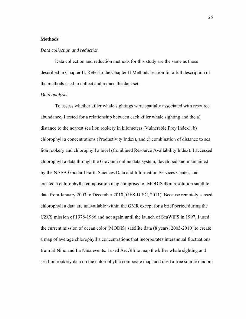
Figure 6: Spatial map of killer whale sightings (1976-1997), combining results of
opportunistic and systematic surveys. Some dots represent more than one sighting.

29
Figure 7: Spatial map of randomly generated data points used for comparison of
available and observed habitat conditions associated with killer whale sightings.
30
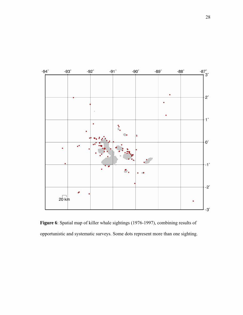
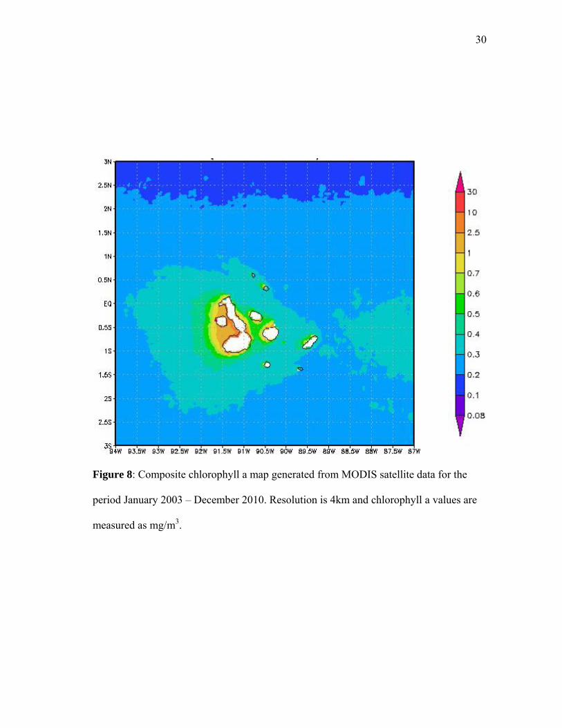
Figure 8: Composite chlorophyll a map generated from MODIS satellite data for the
period January 2003 – December 2010. Resolution is 4km and chlorophyll a values are
measured as mg/m3.
31
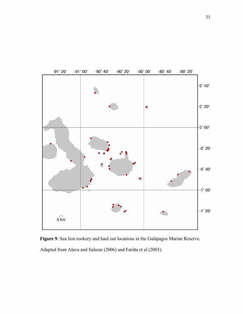
Figure 9: Sea lion rookery and haul out locations in the Galápagos Marine Reserve.
Adapted from Alava and Salazar (2006) and Fariña et al (2003).
32
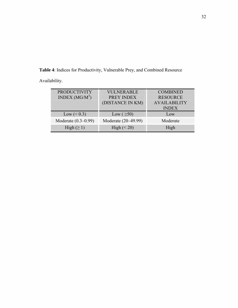
Table 4: Indices for Productivity, Vulnerable Prey, and Combined Resource
Availability.
PRODUCTIVITY INDEX (MG/M3)
VULNERABLE PREY INDEX
(DISTANCE IN KM)
COMBINED RESOURCE
AVAILABILITY INDEX
Low (< 0.3) Low ( ≥50) Low Moderate (0.3–0.99) Moderate (20–49.99) Moderate
High (≥ 1) High (< 20) High

33
Results
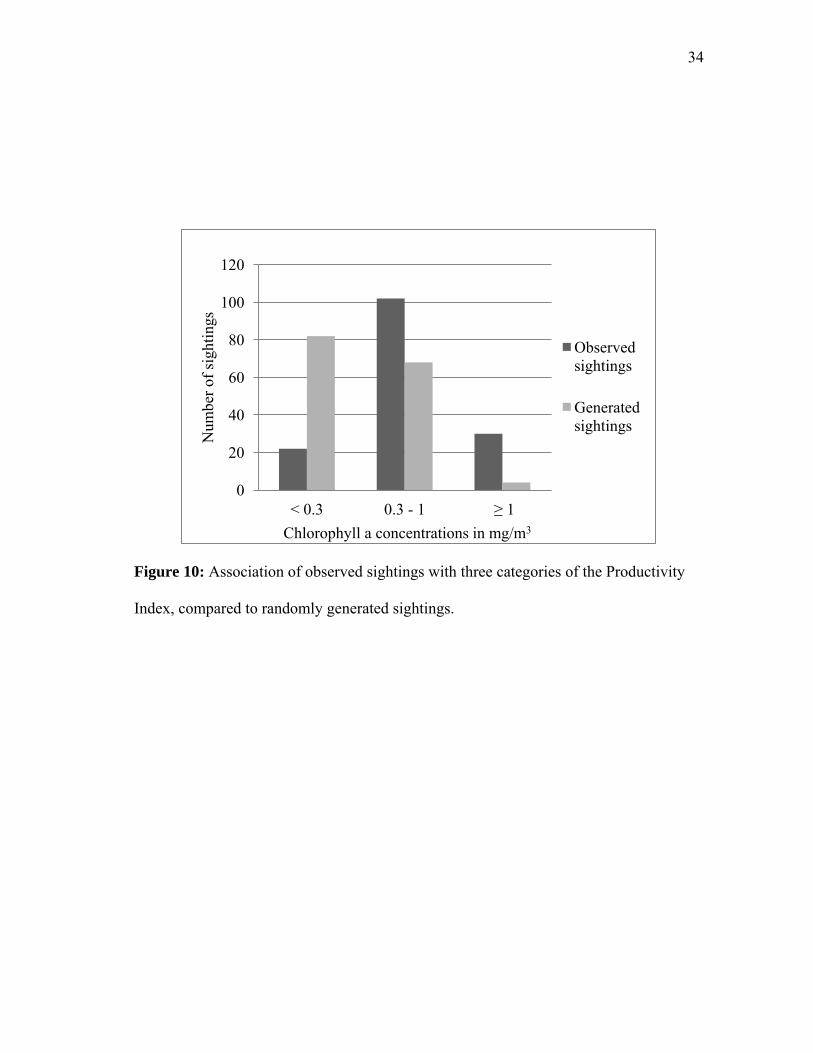
When sightings were tested for an association with the Productivity Index against
the randomly generated points (“chance”), sightings were observed more often than
expected with the Index values of high (binomial z = 4.46, p<0.05) and moderate
(binomial z = 2.61, p<0.05). Sightings were observed less often than expected by chance
with an Index value of low (binomial z = -5.88, p<0.05) (Figure 10, Table 5).
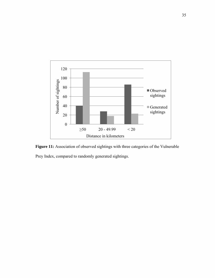
When tested for an association with the Vulnerable Prey Index, sightings were
observed more often than expected by chance with the Index value of high (binomial z =
6.03., p<0.05). When the Index value was moderate sightings were not found more or
less often than by chance (binomial z = 1.47, p>0.05). Sightings were found less often
than expected by chance with the Index value of low (binomial z = -5.90, p<0.05)
(Figure 11, Table 5).
When tested for an association with combined resource availability, sightings
were observed more often than expected by chance when availability was high (binomial
z = 3.64., p<0.05) and moderate (binomial z = 5.87, p<0.05). Sightings were found less
often than expected by chance when the availability was low (binomial z = -6.62,
p<0.05) (Figure 12, Table 5).
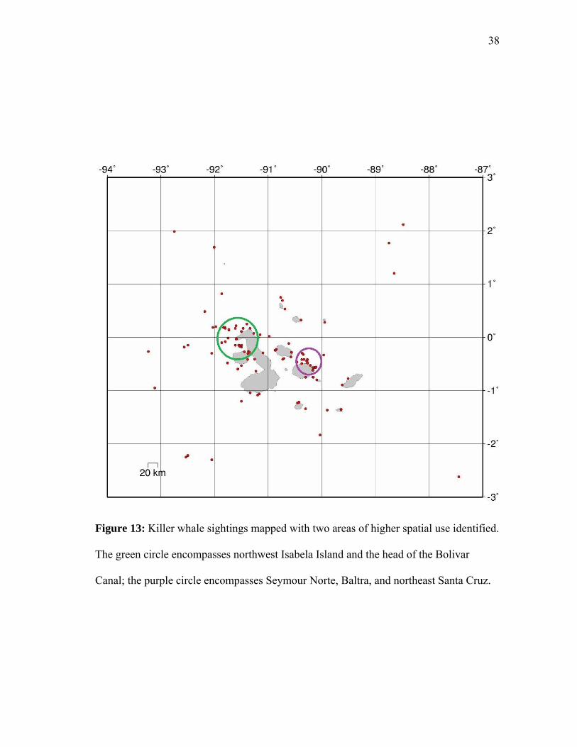
The spatial mapping of the sightings indicated two areas that may be of higher
use by GMR killer whales: northwest Isabela Island and the head of the Bolivar Canal;
and Seymour Norte/Baltra/northeast Santa Cruz (Figure 13).
34
Figure 10: Association of observed sightings with three categories of the Productivity
Index, compared to randomly generated sightings.
0
20
40
60
80
100
120
< 0.3 0.3 - 1 ≥ 1
Num
ber o
f sig
htin
gs
Chlorophyll a concentrations in mg/m3
Observed sightings
Generated sightings
35
Figure 11: Association of observed sightings with three categories of the Vulnerable
Prey Index, compared to randomly generated sightings.
0
20
40
60
80
100
120
≥50 20 - 49.99 < 20
Num
ber o
f sig
htin
gs
Distance in kilometers
Observed sightings
Generated sightings
36
Figure 12: Association of observed sightings with three categories of the Combined
Resource Availability Index, compared to randomly generated sightings.
0
20
40
60
80
100
120
Low Moderate High
Num
ber o
f sig
htin
gs
Combined Resource Availability
Observed sightings
Generated sightings

37
Table 5: Summary of spatial analysis results.
RESOURCE INDEX
RESOURCE INDEX VALUE
SIGHTINGS VS. RANDOM
(BINOMIAL Z SCORE)
PROBABILITY OF SIGHTINGS
OBSERVED COMPARED TO EXPECTED BY
CHANCE Productivity (mg/m3)
Low (< 0.3) -5.88 Less Moderate (0.3-1) 2.61 More High (≥ 1) 4.46 More
Vulnerable Prey (km) Low (≥50) -5.90 Less Moderate (20–49.99) 1.47 Equal High (<20) 6.03 More
Combined Resource Availability
Low -6.62 Less Moderate 5.87 More High 3.64 More
38
Figure 13: Killer whale sightings mapped with two areas of higher spatial use identified.
The green circle encompasses northwest Isabela Island and the head of the Bolivar
Canal; the purple circle encompasses Seymour Norte, Baltra, and northeast Santa Cruz.

39
Discussion
This is the first study to compile multiple data sets of killer whale sightings to
test for a correlation between killer whale sightings and resource distribution in the
GMR. Keeping in mind that research effort varied across time and space for the study
period, these results can provide guidance for future research efforts and sharpen
inductive reasoning about the habitat use of killer whales in the GMR.
Sightings were significantly correlated with the three resource variables tested:
productivity, vulnerable prey, and combined resource availability. Autocorrelation
between sea lion rookeries and higher chlorophyll a did not occur due to limited overlap
in the two variables: sea lion rookeries mostly occur on the interior shores of the islands
while higher levels of chlorophyll a occur on the exterior shores of the western-most
islands. As a result most coastal areas of high chlorophyll a did not correspond to sea
lion rookeries. Despite identifying a relationship between sightings and resource
variables, how killer whales are using these resources, particularly areas with increased
chlorophyll a, is still unknown. Within areas of high chlorophyll a concentrations, killer
whales have been observed predating cetaceans, fish, sharks, and turtles. Unfortunately,
little data are available on these resources with the exception of cetaceans, and the
cetacean data are limited.
Though killer whale sightings were found to have a significant spatial correlation
with sea lion rookeries, few direct observations of killer whales predating sea lions have
been recorded. One predatory report recorded an individual half-beaching on a steep
outcropping composed of boulders (Merlen, 1999), a behavior reminiscent of the feeding

40
tactic employed by the killer whales of Punta Norte, Argentina, and the Crozet Islands
(Lopez and Lopez, 1985; Guinet, 1992; Hoelzel, 1991). Sea lion rookeries in the GMR
are often in very shallow water and protected by volcanic rock outcroppings, which may
be an anti-predator strategy by sea lions to avoid beach-based predation events (Alava,
personal communication, 2011; personal observation, 2011). Adult GMR sea lions, both
male and female, have been observed at least 100 kilometers from shore (personal
observation); if sea lions routinely travel this far from shore, then some killer whales
may have learned to predate them in open water rather than in the shallow coastal zone.
Conversely, the low number of reports of killer whales predating sea lions may
be an indicator that sea lions do not play a significant role in the diet of GMR killer
whales. There exists the possibility that the correlation between sightings and sea lion
rookeries is actually an indicator of habitat quality, and killer whales and sea lions are
both feeding in areas that exhibit a desirable quality, such as an abundance of fish or
cephalopods. Killer whale foraging observations around northeast Santa Cruz, an area
identified in this study with a greater concentration of sea lion rookeries (Figure 9) and
killer whale sightings (Figure 13), are often of killer whales feeding on manta and eagle
rays (Merlen, personal communication 2011).
This study provides insight into the distribution and resource association of GMR
killer whales, but targeted research needs to be conducted to better understand the diet of
killer whales in the GMR. Killer whales have been observed predating a diverse array of
resources, which may be an indicator of the residency patterns of GMR killer whales. If
killer whales in the GMR are comprised of different groups using the region throughout

41
the year, then the discrepancy in prey choice could be a result of the diet specialization
of these diverse groups. If GMR killer whales are found to be composed of multiple
sympatric ecotypes, like those along the Pacific coast of North America, this may result
in distinct prey specializations (Ford et al, 1998). Finally, killer whales in the GMR may
be unspecialized opportunistic predators, such as those found in the Crozet Islands and
around Hawaii (Guinet, 1992; Baird et al, 2006).
Directed research efforts in the two areas circled in Figure 13 as having a greater
abundance of sightings may yield more insight into foraging behavior and social
structure. Additionally, as more research is conducted on the abundance and distribution
of green sea turtles and fish in the GMR, an association between the distribution of these
potential resources and killer whale sightings may be found. Further research needs to be
conducted to determine if the spatial distribution of sightings within the GMR changes
on a temporal basis. In Chapter IV, the results of Chapters II and III will be combined to
test for a shift in the association between sightings and resource availability from the
non-upwelling to upwelling season.

42
CHAPTER IV
TEMPORAL AND SPATIAL INTERACTION
Introduction
Spatial and temporal environmental factors are known to influence the
distribution and habitat use of animals in both marine and terrestrial environments.
Factors such as the photic period, temperature, and primary productivity can all
influence when and where animals are distributed throughout their environment (e. g.
Weir, 2007; Spyrakos, et al, 2011; Wal, et al, 2011). The seasonal abundance of
resources in marine environments varies greatly between different latitudes and is
influenced by both the duration of the photic period and the amount of free nutrients
available (Racault et al, 2012).
In the arctic and sub-arctic waters the photic period changes drastically between
seasons, with the sun being present nearly 24 hours/day during the summer and absent
nearly 24 hours/day during the winter (Sewell and Jury, 2011; Teschke et al, 2011). The
abundance of nutrients increases in the winter when phytoplankton is largely absent,
generating an intense spring and summer bloom when the photic period is long and the
water temperature increases (Sewell and Jury, 2011; Teschke et al, 2011). This results in
short-growing high-amplitude phytoplankton and zooplankton blooms that comprise the
basis of the food-web (Sewell and Jury, 2011; Teschke et al, 2011). Conversely, in the
tropics and sub-tropics the photic period remains fairly constant throughout much of the
year and the availability of nutrients act as the limiting factor in resource abundance

43
(Sewell and Jury, 2011; Teschke et al, 2011; Racault et al, 2012). In these regions
blooms are generally characterized as long-growing with low-amplitude (Racault et al,
2012). Along coastal zones blooms may be more intense due to the forcing of nutrients
to surface through upwelling, but in open-ocean pelagic ecosystems nutrients remain
submerged below the level at which they can be utilized by phytoplankton (Sewell and
Jury, 2011; Teschke et al, 2011; Racault et al, 2012).
The Galápagos Marine Reserve is a tropical marine environment with greater
than average primary productivity due to seasonal upwelling and long photic periods
(Palacios, 2004), Sweet et al, 2007; Schaeffer et al, 2008). Increased chlorophyll a levels
enable increased levels of lower trophic level organisms, which in turn increase the
abundance of mid-level trophic organisms (Hunt, 2006; Alava, 2009). Many of the prey
items GMR killer whales have been observed predating are mid-level trophic organisms
(e. g. fish, cephalopods, rays) (Alava, 2009). GMR killer whale sightings are known to
be spatially associated with areas of high chlorophyll a concentrations and sea lion
rookeries, however little is known about their diet or how that diet may change
temporally (Merlen, 1999, Chapter III). Seasonal patterns of chlorophyll a
concentrations could be a driving factor if GMR killer whale sightings are found to
spatially shift with respect to temporal variability.
Killer whales have also been observed predating sea lions, a mobile upper level
trophic organism, and the results of Chapter III indicate that the sighting distribution of
killer whales is correlated with sea lions. Due to a lack of strong photoperiodic change,
Galápagos sea lions do not exhibit the seasonal breeding synchrony common among

44
pinnipeds, and thus produce offspring year round (Villegas-Amtmann et al, 2009). If
killer whales are foraging on resources influenced by seasonal upwelling, then they may
prey switch to feed on sea lions when primary productivity decreases, resulting in a shift
in the spatial distribution of sightings.
Although killer whales in the GMR have been observed predating a wide range
of resources, from cetaceans to sea turtles, but it is unknown if there is dietary
specialization within groups or social units (Merlen, 1999; Palacios, 2003, Alava and
Merlen, 2009; Merlen, personal communication 2011). If GMR killer whales are
specialized foragers then they may shift their distribution to follow their prey, or prey-
shift between one or two important resources with different spatial distributions. If they
are generalist predators, then there may be no significant shift in spatial distribution.
The aim of this chapter is to build on the results of Chapters II and III to gain a
better understanding of how spatial sighting distribution may be influenced by temporal
variability. To achieve this, I analyzed 20 years of data involving temporal and spatial
distribution collected via ship-board line-transect surveys and observations of
opportunity by an observer network.

45
Methods
Data collection and reduction
The data evaluated in this chapter are the same evaluated in Chapters II and III.
Refer to Chapter II Methods for information on the data collection and reduction
methods employed.
Data analysis
To assess whether the spatial distribution of killer whale sightings changed
temporally, I tested for a relationship between each killer whale sighting per season
(non-upwelling and upwelling) and the a) distance to the nearest sea lion rookery in
kilometers, b) chlorophyll a level, and c) combination of distance to sea lion rookery and
chlorophyll a level. I accessed chlorophyll a data through the Giovanni Online Data
System, developed and maintained by the NASA Goddard Earth Sciences Data and
Information Services Center and created a chlorophyll a map from MODIS 4km satellite
data for each month of 2004 (GES-DISC, 2011). Because remotely sensed chlorophyll a
data from the GMR were not routinely collected during the study period, I selected a
year for analysis with available satellite coverage that exhibited no strong El Niño or La
Niña trends. ArcGIS was used to map sea lion rookery data and the ArcGIS measuring
tool to measure the distance in kilometers from each sighting to the nearest sea lion
rookery. I then measured the level of chlorophyll a at each sighting for each
corresponding month, such that if a sighting was recorded for January for any year of the
study period, I mapped it on the January 2004 chlorophyll a map.

46
Sightings were assigned to a Productivity, Vulnerable Prey, and Combined
Resource Availability Index as described in Chapter III (see Chapter III Methods and
Table 3). The Productivity Index measured the level of chlorophyll a present at each
sighting and the Vulnerable Prey Index measured the distance in kilometers from each
sighting to the nearest sea lion rookery. The Combined Resource Availability Index
value for each sighting was generated by combining the values from the Productivity and
Vulnerable Prey Indices. I used a binomial z test (Bakeman and Gottman, 1986) to
compare the probability of co-occurrence of killer whale sightings per season for each
resource category. Because the number of sightings each season are not equal, I
measured whether the probability of sightings in the upwelling season occurred more
than, less than, or equal to the probability of sightings observed in the non-upwelling
season.

47
Results
Upwelling and non-upwelling sightings were observed with equal
probability for all three levels of the Productivity Index: high (binomial z = -0.05,
p>0.05); moderate (binomial z = -0.27, p>0.05); low (binomial z = 0.58, p>0.05) (Figure
14, Table 6). Sightings between the two seasons were also found to occur with equal
probability for all three categories of the Vulnerable Prey Index: high (binomial z = 1.54,
p>0.05); moderate (binomial z = -0.77, p>0.05); and low (binomial z = -1.60, p>0.05)
(Figure 15, Table 6). However, there was a difference in the occurrence of upwelling
sightings compared to non-upwelling sightings for the Combined Resource Availability
Index. Upwelling sightings were observed with equal probability for the high (binomial
z = 0.56, p>0.05) and moderate (binomial z = 1.73, p>0.05) resource levels and less
often than expected for the low level (binomial z = -3.17, p<0.05) (Figure 16, Table 6).
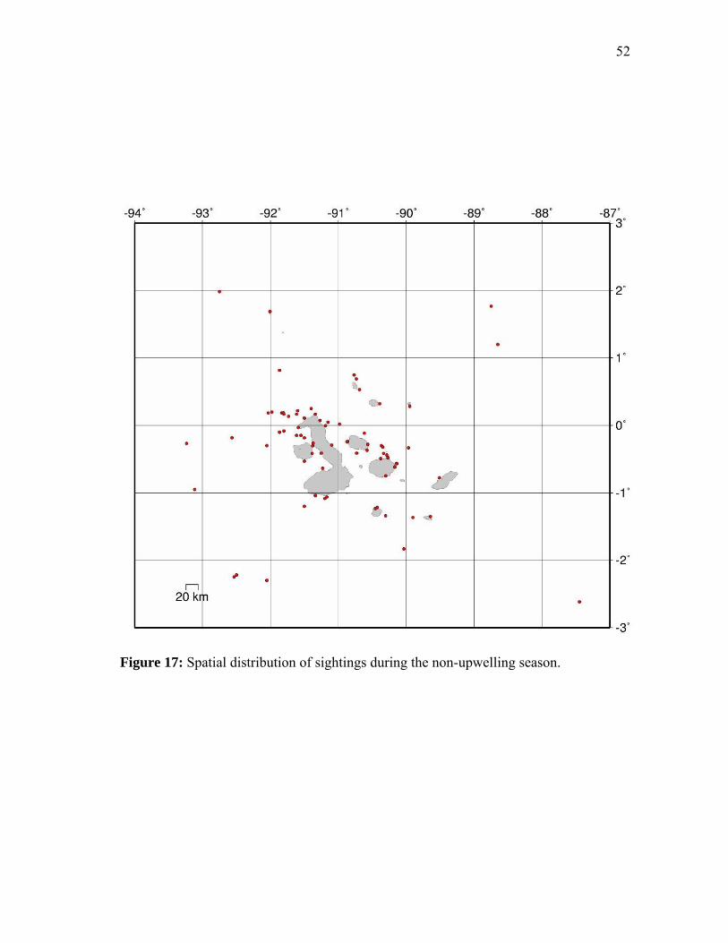
The spatial mapping of sightings in the non-upwelling (Figure 17) and upwelling (Figure
18) seasons provided a clear visualization of the decrease in sightings in areas of low
resource value during the upwelling season compared to the non-upwelling season.
Sightings in the non-upwelling season were more scattered within the study area and
sightings were more clustered in areas of increased combined resource productivity for
the upwelling season.

48
Figure 14: Non-upwelling versus upwelling sightings per level of the Productivity
Index.
0
20
40
60
80
< 0.3 0.3 - 1 ≥ 1
Num
ber o
f sig
htin
gs
Chlorophyll a concentrations in mg/m3
Non-upwelling sightings
Upwelling sightings

49
Figure 15: Non-upwelling versus upwelling sightings per level of the Vulnerable Prey
Index.
0
10
20
30
40
50
60
≥50 20 - 49.99 < 20
Num
ber o
f sig
hitn
gs
Distance in kilometers
Non-upwelling sightings
Upwelling sightings

50
Figure 16: Non-upwelling versus upwelling sightings per level of the Combined
Resource Availability Index.
0
20
40
60
80
Low Moderate High
Num
ber o
f sig
htin
gs
Resource Availability
Non-upwelling sightings
Upwelling sightings

51
Table 6: Summary of temporal-spatial analysis results
RESOURCE INDEX
RESOURCE INDEX VALUE
UPWELLING VS NON-
UPWELLING SIGHTINGS
(BINOMIAL Z SCORE)
PROBABILITY OF UPWELLING
SIHTINGS VS NON-
UPWELLING SIGHTINGS
Productivity (mg/m3) Low (< 0.3) 0.58 Equal Moderate (0.3-1) -0.27 Equal High (≥ 1) -0.05 Equal
Vulnerable Prey (km) Low (≥50) -1.6 Equal Moderate (20–49.99) -0.77 Equal High (<20) 1.54 Equal
Combined Resource Availability
Low -3.17 Less Moderate 1.73 Equal High 0.56 Equal
52
Figure 17: Spatial distribution of sightings during the non-upwelling season.

53
Figure 18: Spatial distribution of sightings during the upwelling season.
54
Discussion
This study builds on the temporal and spatial results from Chapters II and III, and
is the first study to synthesize multiple sets of killer whale sightings in the GMR and test
for a spatial shift in sightings with respect to temporal change. In Chapter II, I reported
that killer whales are present in the GMR all year, with a slight increase in expected
sightings in the peak upwelling period of August – November. In Chapter III, killer
whale sightings were shown to be spatially associated with sea lion rookeries
(Vulnerable Prey Index), areas of high chlorophyll a concentrations (Productivity Index),
and areas with resource overlap (Combined Resource Availability Index). With the
understanding that data collection methods varied in effort across time and space, the
results of this study provide insight into the temporal and spatial habitat use of killer
whales in the GMR.
Sighting distribution did not change between seasons with respect to the
Productivity, Vulnerable Prey, or Combined Resource Availably Indices. However,
during the peak upwelling period identified in Chapter II, killer whale sightings occurred
less often than expected in areas of low productivity. It is uncertain why killer whale
distribution changes for this variable, but it could be an indicator that important
resources, such as migratory whales, may be clustering around areas of high productivity
and thus influencing a shift in killer whale distribution.
These results indicate that killer whales are not making a significant prey switch
(e. g. sea lions to fish) between seasons. This could be a result of year-round
unspecialized foraging in areas of higher abundance, as hypothesized in Merlen (1999)

55
and Chapter III. If killer whales in the GMR are comprised of multiple populations
passing through the region throughout the year, then physical drivers outside of the
scope of this study may be driving killer whales to forage more heavily in areas of high
resource abundance during upwelling.
This study demonstrates that killer whales sightings are spatially associated with
resources, though there seems to be little temporal effect on that association. That
sightings occurred less often in areas of low productivity during upwelling seasons is
interesting, but more research needs to be conducted to better understand what this
means regarding killer whale residency and behavioral ecology.
56
CHAPTER V
SUMMARY AND CONCLUSIONS
Summary
The goal of this study was to answer three basic questions about killer whales in
the Galápagos Marine Reserve and surrounding waters: a) is there a temporal pattern to
killer whale sightings; b) are sightings spatially associated with potential resources
(chlorophyll a or sea lion rookeries); and c) if sightings are spatially associated with
resources, does the spatial distribution of sightings change temporally? Sighting data
were collected between 1976 and 1997 via shipboard line-transect survey and
opportunistic sightings by an observer network (n = 154).
In Chapter II, I tested for a temporal pattern to killer whale sightings in three
different ways: i) bi-seasonal variation, ii) inter-annual ENSO influence and iii) a
combination of seasonal and ENSO event influence. I found that sightings occurred in
every month of the year, though not every month every year, and were roughly equally
distributed between the non-upwelling and upwelling seasons. The strength of ENSO
events did not have a significant influence on the number of sightings from year to year.
Sightings were found to occur more often than expected by chance in the peak upwelling
series of August – October and August – November when the MEI was within one
standard deviation of the norm.
In Chapter III, I tested for a spatial association between sightings and three
resource variables: i) chlorophyll a concentrations (Productivity Index), ii) distance to

57
sea lion rookeries (Vulnerable Prey Index) and iii) the combined value of chlorophyll a
and distance to sea lion rookeries (Combined Resource Availability Index). Sightings
were found to occur more often than expected by chance when Productivity Index levels
were high (≥ 1mg/m3) and moderate (0.3 – 0.99mg/m3) and less often than expected by
chance when Productivity Index levels were low (<0.3mg/m3). Sightings occurred more
often than expected by chance when <20km from sea lion rookeries, with equal
occurrence of chance 20 – 49km from rookeries, and less than expected by chance
≥50km from rookeries. When these two resource variables were explored in more detail
sightings were found to occur more often than expected in areas of high and moderate
combined resource availability, and less often than expected in areas with low combined
resource availability. Additionally, sightings were more concentrated in two areas:
northwest Isabela Island and the head of the Bolivar Canal; and Seymour Norte, Baltra,
and northwest Santa Cruz.
In Chapter IV, the results from Chapters II and III were used to test for a spatial
change in sighting distribution with respect to temporal variability. Using the four month
upwelling peak identified in Chapter II (August – November), I compared the number of
sightings per level of resource category for each season. I found that the number of
sightings for both seasons did not significantly shift for either the Productivity or
Vulnerable Prey Indices. The number of sightings for high and moderate Combined
Resource Availability Index levels did not change between seasons, but sightings were
significantly less likely to occur in areas of low combined resource availability in the
upwelling season.
58
Conclusions
The results of this study show killer whales are present in the Galápagos Marine
Reserve throughout the year. In most years, killer whale presence does not appear to be
influenced by El Niño Southern Oscillation Events. Sighting abundance did increase
during the peak upwelling months when the MEI was normal, but this could be an
artifact of increased boat activity and thus more opportunities to sight killer whales.
Because resources are more abundant during times of increased productivity there may
be more observers (e.g. fishermen, divers) on the water to use those resources, thus
increasing the number of sightings. This is not conclusive but should be considered
when interpreting these results. The residency patterns of GMR killer whales remain
unsolved and require further research. That sightings were recorded every month is a
strong indicator that the presence of killer whales in the GMR is not limited to times of
high productivity or resource pulses. However, the residency patterns of killer whales
are still unknown, and there may exist a single resident population, multiple resident and
transient populations, or that killer whales observed in the GMR may be part of the ETP
population and routinely visit the region.
The correlation between sightings and areas of primary productivity implies that
killer whales are foraging in areas of increased productivity where mid-trophic level
resources may be more abundant. Foraging observations of killer whales in these areas
indicate they are predating rays, sharks, fish, and other cetaceans (Arnbom et al, 1987;
Merlen, 1999; Palacios, 2003; Alava, 2009), which may be in the area due to the
increased availability of prey resources. While sightings were found to be spatially

59
correlated with sea lion rookeries, it needs to be remembered that correlation does not
equal causation. Reports of GMR killer whales attacking sea lions and fur seals have
been documented, but not with any great abundance (Merlen, 1999; Merlen, personal
communication 2010). There exists the possibility that killer whales and sea lions are
sympatric populations utilizing the same areas due to a desirable habitat quality, such as
an abundance of fish or cephalopod resources. If killer whales in the GMR are later
found to be comprised of different ecotypes, there may well be an ecotype that predates
sea lions and a type that does not. The greater number of sightings in northwest Isabela
Island and the head of the Bolivar Canal, and Seymour Norte, Baltra, and northeast
Santa Cruz each coincide with increased resource availability. The northwest
Isabela/Bolivar Canal region is an area of increased upwelling and chlorophyll a
concentrations, while the area of northeast Santa Cruz is the location of many sea lion
rookeries.
When examining whether the spatial distribution of sightings may have a
temporal component, I found significantly less sightings occurred in areas of low
productivity in the upwelling season, when resources are likely most abundant. This may
mean that if most killer whales in the GMR are transient or migratory they may be using
the area more for foraging and less for travelling during these times. More research
needs to be conducted to better understand how killer whales are using the GMR.

60
Recommendations for future research
While this study answers basic questions about killer whale presence in the
Galápagos Marine Reserve and surrounding waters, future research is needed to gain a
better understanding of their behavioral ecology. I identified two locations in the GMR
(northwest Isabela Island and west Baltra/Seymour Norte) where killer whales are more
frequently sighted, which may prove to be productive areas to base future research
projects. Increased boat-based survey effort in both locations could yield important data
on social interactions, predatory behavior, and provide opportunities to acquire skin
sloughs and fecal matter for genetic and physiology studies. Photos of individuals could
be used to generate a photo ID catalog to assist in identifying social units and provide
more information about killer whale residency in the region. Stationary underwater
acoustic devices could be used to monitor killer whale presence in an area and to collect
vocalization data. Though more invasive, the use of satellite tags and biopsy darts could
be effective tools to gain insight into killer whale movement patterns, diet, health, and
genetics.
This study focused on the affects of bottom-up influences on killer whales (e. g.
resource distribution), but future studies focused on the top-down influence of killer
whales on the environment could be useful. Examples of this include comparing the
behavior and feeding tactics of sea lions within killer whale “hot spots” and those from
other locations, or monitoring changes to migrant whale behavior when in the vicinity of
killer whales or in areas where killer whales are more frequently observed. These types
of studies may provide additional clues to killer whale foraging and resource use.

61
REFERENCES
ALAVA, J. J. (2009) Carbon productivity and flux in the marine ecosystems of the
Galápagos Marine Reserves based on cetacean abundances and trophic indices. Revista
de Biologia Marina y Oceanografia 44(1): 109 – 122.
ALAVA, J.J. AND MERLEN, G. (2009) Video-documentation of a killer whale
(Orcinus orca) predatory attack on a giant manta (Manta birostris) in the Galápagos
Islands. Latin American Journal of Aquatic Mammals 7(1-2): 81-84.
ALAVA, J. J. AND SALAZAR, S. (2006) Status and Conservation of Otariids in
Ecuador and the Galápagos Islands. Pages 495 – 519 in TRITES, A. W., ATKINSON,
S. K., DEMASTER, D. P, FRITZ, L. W., GELATT, T. S., REA, L. D., AND WYNNE,
K. M. (Eds) Sea Lions of the World Alaska Sea Grant College Program, University of
Alaska Fairbanks. Fairbanks, Alaska, USA.
ANDREWS, R. D., PITMAN, R. L., AND BALLANCE, L. T. (2008) Satellite tracking
reveals distinct movement patterns for Type B and Type C killer whales in the southern
Ross Sea, Antarctica. Polar Biology 31: 1461 – 1468.
ARNBOM, T., PAPASTAVROU, V., WEILGART, L. S., AND WHITEHEAD, H.
(1987) Sperm whales react to an attack by killer whales. Journal of Mammalogy 68(2):
450 – 453.

62
BAIRD, R. W., MCSWEENEY, D. J., BANE, C., BARLOW, J., SALDEN, D. R.,
ANTOINE, L. K., LEDUC, R. G., AND WEBSTER, D. L. (2006) Killer whales in
Hawaiian waters: information on population identity and feeding habits. Pacific Science
60(4): 523- 530.
BAKEMAN, R. AND GOTTMAN, J.M. (1986) Observing interaction: an introduction
to sequential analysis. Cambridge: Cambridge University Press. p. 118-168.
BALLANCE, L. T., PITMAN, R. L. AND FIEDLER, P. C. (2006). Oceanographic
influences on seabirds and cetaceans of the eastern tropical Pacific: A review. Progress
in Oceanography 69(2-4): 360-390.
BARRETT-LENNARD, L. G., MATKIN, C. O., DURBAN, J. W., SAULITIS, E. L.,
AND ELLIFRIT, D. (2011) Predation on gray whales and prolonged feeding on
submerged carcasses by transient killer whales at Unimak Island, Alaska. Marine
Ecology Progress Series 421: 221-241.
BENSON, S. R., CROLL, D. A., MARINOVIC, B. B., CHAVEZ, F. P., AND
HARVEY, J. T. (2002) Changes in the cetacean assemblages of a coastal upwelling
ecosystem during El Niño 1997 – 1998 and La Niña 1999. Progress in Oceanography
54: 279 – 291.

63
DAHLHEIM, M. E. (1997) A Photographic Catalog of Killer Whales, Orcinus orca,
from the Central Gulf of Alaska to the Southeastern Bering Sea. NOAA Technical
Reports NMFS 131.
DAHLHEIM, M. E., SCHULMAN-JANIGER, A., BLACK, N., TERNULIO, R.,
ELLIFRIT, D., AND BALCOMB, K. C. (2008). Eastern temperate North Pacific
offshore killer whales (Orcinus orca): Occurrence, movement, and insights into feeding.
Marine Mammal Science 24(3): 719 – 729.
DURBAN, J., ELLIFRIT, D., DAHLHEIM, M., WAITE, J., MATKIN, C., BARRETT-
LENNARD, L., ELLIS, G., PITMAN, R., LEDUC, R., AND WADE, P. (2010)
Photographic mark-recapture analysis of clustered mammal-eating killer whales around
the Aleutian Islands and Gulf of Alaska. Marine Biology 154: 1591-1604.
DURBAN, J.W. AND PITMAN, R. L. (2011) Antarctic killer whales make rapid,
round-trip movements to subtropical waters: evidence for physiological; maintenance
migrations? Biology Letters doi: 10.1098/rsbl.2011.0875
64
EDGAR, G.J., BANKS, S.A., BRANDT, M., BUSTAMANTE, R. H., CHIRIBOGA,
A., EARLE, S. A., GARSKE, L. E., GLYNN, P. W., GROVE, J. S., HENDERSON, S.,
HICKMAN, C. P., MILLER, K. A., RIVERA, F., AND WELLINGTON, G. M. (2010)
El Niño, grazers, and fisheries interact to greatly elevate extinction risk for Galápagos
marine species. Global Change Biology 16: 2876-2890
ESRI (2011). Available at <http://arcscripts.esri.com/details.asp?dbid=12098>
Consulted 3 March, 2011)
ESRL (2011). Earth Systems Research Laboratory. Available online at
<http://www.esrl.noaa.gov/psd/enso/mei/table.html> Consulted 19 February 2011.
FARIÑA, J. M., SALAZAR, S., WALLEM, P., WITMAN, J. AND ELLIS, J. S. (2003)
Nutrient exchanges between marine and terrestrial ecosystems: the case of the
Galápagos sea lion (Zalophus wollebaeki). Journal of Animal Ecology 72:873–887.
FLORES-RAMIREZ, S., URBAN, J., VILLAREAL-CHAVEZ, G., AND VALLES-
JIMENEZ, R. (1996) Spatial and temporal changes in the cetacean community structure
at Bahia de la Paz, B.C.S., Mexico (1988-1991). Ciencias Marinas 22(2): 151 – 173.

65
FOOTE, A. D., SIMILA, T., VIKINGSSON, G. A., STEVICK, P. T. (2010) Movement,
site fidelity and connectivity in a top marine predator, the killer whale. Evolution and
Ecology 24: 803 – 814.
FORD, J. K. B., ELLIS, G. M., BARRETT-LENNARD, L. G., MORTON, A. B.,
PALM, R. S., AND BALCOMB, K. C. (1998) Dietary specialization in two sympatric
populations of killer whales (Orcinus orca) in coastal British Columbia and adjacent
waters. Canadian Journal of Zoology 76(8): 1456 – 1471.
GARDNER, S. C. AND CHAVEZ-ROSALES, S. (2000) Changes in the relative
abundance and distribution of gray whales (Eschrichtius robustus) in Magdelena Bay,
Mexico during an El Niño event. Marine Mammal Science 16(4): 728 – 738.
GES-DISC (2011). Goddard Earth Sciences Data and Information Services Center
Interactive Online Visualization and Analysis Infrastructure. Available at
<http://disc.sci.gsfc.nasa.gov/giovanni#maincontent> Consulted 19 February, 2011; 26
March, 2011.
HAUSER, D. D. W., LOGSDON, M. G., HOLMES, E. E., VANBLARICOMB, G. R.,
AND OSBORNE, R. W. (2007) Summer distribution patterns of southern resident killer
whales Orcinus orca: core areas and spatial segregation of social groups. Marine
Ecology Progress Series 351: 301 – 310.

66
GUINET, C. (1992) Comportement de chasse des orques (Orcinus orca) autour des iles
Crozet. Canadian Journal of Zoology 70(9): 1656 – 1667.
GUINET C., BARRETT-LENNARD L. G., LOYER B. (2000) Co-ordinated attack
behavior and prey sharing by killer whales at Crozet Archipelago: strategies for feeding
on negatively-buoyant prey. Marine Mammal Science 16: 829–834.
HOELZEL, A. R. (1991) Killer whale predation on marine mammals at Punta Norte,
Argentina; food sharing, provisioning, and foraging strategy. Behavioral Ecology and
Sociobiology 29: 197- 204.
HUNT, G. L. (2006) Evidence for bottom-up control of upper-trophic-level marine
populations. Pages 50-64 in ESTES, J.A., DEMASTER, D.P., DOAK, D. F.,
WILLIAMS, T.M., AND BROWNELL, R. L. (Eds) Whales, Whaling, and Ocean
Ecosystems. University of California Press. Berkeley and Los Angeles California, USA.
JEGLINSKI, J. W. E, WERNER, C., GOETZ, K. T., COSTA, D. P., AND
TRILLMICH, F. (2011) Niche competition: do juvenile Galápagos sea lions compete
with adult Galápagos fur seals? 19th Biennial Conference on the Biology of Marine
Mammals. Tampa, Florida, USA. November 28 – December 3, 2011.
67
KARNAUSKAS, K.B., MURTUGUDDE, R., AND BUSALACCHI, A.J. (2010)
Observing the Galápagos-EUC interaction: insights and challenges. Journal of Physical
Oceanography 40: 2768-2777.
KRAHN, M. M., HERMAN, D. P., MATKIN, C. O., DURBAN, J. W., BARRETT-
LENNARD, L., BURROWS, D. G., DAHLHEIM, M. E., BLACK, N., LEDUC, R. G.,
AND WADE, P. R. (2007) Use of chemical tracers in assessing the diet of foraging
regions of eastern North Pacific killer whales. Marine Environmental Research 63: 91 –
114.
LOPEZ, J. C. AND LOPEZ, D. (1985) Killer whales (Orcinus orca) of Patagonia, and
their behavior of intentional stranding while hunting nearshore. Journal of Mammalogy
66(1): 181 – 183.
MATKIN C. O., BARRETT-LENNARD L. G., YURK H, ELLIFRIT D. K., TRITES A.
W. (2007) Ecotypic variation and predatory behavior of killer whales (Orcinus orca) in
the eastern Aleutian Islands, Alaska. Fish Bulletin 105:74–87.
MATTHEWS, C. J. D., LUQUE, S. P., PETERSON, S. D., ANDREWS, R., D.,
FERGUSON, S. H. (2011) Satellite tracking of a killer whale (Orcinus orca) in the
eastern Canadian Arctic documents ice avoidance and rapid, long-distance movement to
the North Atlantic. Polar Biology 34: 1091 – 1096.
68
MERLEN, G. (1999) The orca in the Galápagos: 135 sightings. Noticias de Galápagos
60: 2-8.
MERLEN, G. (2000) Nocturnal acoustic locations of the Galápagos fur seal
Arctocephalus galapagoensis. Marine Mammal Science 16(1): 248 – 253.
OLSON, P. A. AND GERRODETTE, T. (2008) Killer Whales of the Eastern Tropical
Pacific: A Catalog of Photo-Identified Individuals. NOAA Technical Memorandum
NMS-SWFSC-428.
PALACIOS, D.M. (2003) Oceanographic conditions around the Galápagos Archipelago
and their influence on cetacean community structure. Ph.D. Dissertation, Oregon State
University, Corvallis, Oregon. 178 pp.
PALACIOS, D. M. (2004) Seasonal patterns of sea-surface temperatures and ocean
color around the Galápagos: regional and local influences. Deep Sea Research II 51: 43
– 57.
PISTORIUS, P. A., TAYLOR, F. E., LOUW, C., HANISE, B., BESTER, M. N., DE
WET, C., DU PLOOY, A., GREEN, N., KLASEN, S., PODILE, S., AND SCHOEMAN
(2002) Distribution, movement, and estimated population size of killer whales at Marion
Island, December 2000. South African Journal of Wildlife Research 32(1): 86 – 92.

69
RACAULT, M. F., LA QUERE, C., BUITENHUIS, E., SATHYENDRANATH, S.,
AND PLATT, T. (2012) Phytoplankton phenology in the global ocean. Ecological
Indicators 14(1): 152-163
REISINGER, R. R., DE BRUYN, P. J. N., TOSH, C. A., OOSTHUIZEN, W. C.,
MUFANADZO, N. T., AND BESTER, M. N. (2011) Prey and seasonal abundance of
killer whales at sub-Antarctic Marion Island. African Journal of Marine Science 33(1):
99 – 105.
SALVADEO, C. J., FLORES-RAMIREZ, S., GOMEZ-GALLARDO, A., MACLEOD,
U., LLUCH-BELDA, D., JUAME-SCHINKEL, S. AND URBAN, J. (2011) Bryde’s
whale (Balaenoptera edeni) in the southwestern Gulf of California: Relationship with
ENSO variability and prey availability. Ciencias Marinas 37(2): 215 – 225.
SCHAEFFER, B.A., MORRISON, J.M., KAMYKOWSKI, D., FELDMAN, G. C., XIE,
L., SWEET, W., MCCULLOCK, A., AND BANKS, S. (2008) Phytoplankton biomass
distribution and identification of productive habitats within the Galápagos Marine
Reserve by MODIS, a surface acquisition system, and in situ measurements. Remote
Sensing of Environment 112: 3044-3054

70
SEWELL, M. A. AND J. A. JURY. (2011) Seasonal patterns in diversity and abundance
of the High Antarctic meroplankton: Plankton sampling using a Ross Sea desalination
plant. Limnology and Oceanography 56(5): 1667-1681.
SMITH, S. C. AND WHITEHEAD, H. (1993) Variations in the feeding success and
behavior of Galápagos sperm whales (Physeter-macrocephalus) as they relate to
oceanographic conditions. Canadian Journal of Zoology-Revue Canadienne De
Zoologie 71(10): 1991-1996.
SORISIO, L. S., DE MADDALENA, A., AND VISSER, I. N. (2006) Interaction
between killer whales (Orcinus orca) and hammerhead sharks (Sphyrna sp.) in
Galápagos waters. Latin American Journal of Aquatic Mammals 5(1): 69 -71
SPYRAKOS, E., SANTOS-DINIZ, T. C., MARTINEZ-IGLESIAS, G., TORRES-
PALENZUELA, J. M., AND PIERCE, G. J. (2011) Spatiotemporal patterns in marine
mammal distribution in coastal waters of Galicia, Spain. Hydrobiologia 670: 87 – 109.
SWEET, W.V., MORRISON, J.M., KAMYKOWSKI, D., SCHAEFFER, B. A.,
BANKS, S., AND MCCULLOCH, A. (2007) Water mass seasonal variability in the
Galápagos Archipelago. Deep-Sea Research I 54: 2023-2035

71
TESCHKE, M., WENDT, S, KAWAGUCHI, S., KRAMER, A, AND MEYER, B.
(2011) A circadian clock in Antarctic krill: an endogenous timing system governs
metabolic output rhythms in the euphausid species Euphausia superb. PLoS One 6(10):
DOI: 10.1371/journal.pone.0026090
TRILLMICH, F. AND LIMBERGER, D. (1985) Drastic effects of El Niño on
Galápagos Pinnipeds. Oecologia 67(1): 19-22.
VARGAS, F. H., LACY, R. C., JOHNSON, P. J., STEINFURTH, A., CRAWFORD, R.
J. M., BOERSMA, P. D., AND MACDONALD, D. W. (2007) Modeling the effect of
El Niño on the persistence of small populations: The Galápagos penguin as a case study.
Biological Conservation 137(1): 138-148.
VILLEGAS-AMTMANN, S., ATKINSON, S, AND COSTA, D. P. (2009) Low
synchrony in the breeding cycle of Galápagos sea lions revealed by seasonal
progesterone concentrations. Journal of Mammalogy 90(5): 1232 – 1237.
WADE, P. R. AND GERRODETTE, T. (1993) Estimates of Cetacean Abundance and
Distribution in the Eastern Tropical Pacific. Reports of the International Whaling
Commission 43:477 – 494.

72
WAL, E. V., MCLOUGHLIN, P. D., AND BROOK, R. K. (2011) Spatial and temporal
factors influencing sightability of elk. The Journal of Wildlife Management 75(6): 1521
– 1526.
WEIR, C. R., STOCKIN, K. A., AND PIERCE, G. J. (2007) Spatial and temporal trends
in the distribution of harbor porpoises, white-beaked dolphins and minke whales off
Aberdeenshire (UK), north-western North Sea. Journal of the Marine Biology
Association of the UK 87: 327 – 338.
73
VITA
Kerri Jean Smith received her Bachelor of Science degree in marine biology
from Texas A&M University at Galveston in 2008. She entered the Marine Biology
Interdisciplinary Program at Texas A&M in August 2009 and will receive the Master of
Science degree in May 2012. She is broadly interested in the behavioral ecology and
ecophysiology of marine predators, particularly marine mammals, seabirds and sharks;
the complex nature of marine ecosystems; and marine biodiversity and conservation. She
plans to pursue a PhD and continue marine ecosystem research.
Ms. Smith can be reached by e-mail to [email protected] and mail to
2258 TAMU, College Station, TX 77843.


