

Electronic copy available at: http://ssrn.com/abstract=1363957
Smoothing, Persistence, and Hedge Fund PerformanceEvaluation
Jing-zhi Huang, John Liechty, and Marco Rossi∗
March 18, 2009
Abstract
Hedge funds often hold illiquid assets whose true value is slowly reflected in reportedreturns. As a result, reported returns can become a smoothed version of true realizedreturns and, thus, bias the evaluation of hedge fund performance. To address thisproblem, we provide a Bayesian framework for the performance evaluation of managedportfolios that accounts for: return smoothing; time-variation in performance and fac-tor loadings; and the often short-lived nature of such portfolios. Using simulated data,we estimate several restricted versions of our model and find that smoothing affects per-formance evaluation more than time-variation or the fact that many of these funds areshort-lived. We apply the model to equity hedge funds and find that, even for theserelatively liquid strategies, smoothing causes an upward bias in excess performancemeasures, e.g. the fund’s α, and a downward bias in risk measures. In particular, weshow that a moderate level of smoothing can cause the standard OLS α to over-estimateequity funds’ abnormal performance by more than 1% annually.
Keywords: Hedge funds, return smoothing, performance persistence, Bayesiananalysis, time-varying betas.
∗Corresponding author: 326B Business, Department of Finance, Pennsylvania State University; Email:[email protected]; Tel: 814-865-2446. The other authors are also from the Pennsylvania State University(department of Finance, and Marketing respectively). We thank Vikas Argod from the High PerformanceComputing Group at Penn State for his help with parallel computing.

Electronic copy available at: http://ssrn.com/abstract=1363957
Smoothing, Persistence, and Hedge Fund Performance Evaluation
Abstract
Hedge funds often hold illiquid assets whose true value is slowly reflected in reported returns.
As a result, reported returns can become a smoothed version of true realized returns and,
thus, bias the evaluation of hedge fund performance. To address this problem, we provide
a Bayesian framework for the performance evaluation of managed portfolios that accounts
for: return smoothing; time-variation in performance and factor loadings; and the often
short-lived nature of such portfolios. Using simulated data, we estimate several restricted
versions of our model and find that smoothing affects performance evaluation more than
time-variation or the fact that many of these funds are short-lived. We apply the model
to equity hedge funds and find that, even for these relatively liquid strategies, smoothing
causes an upward bias in excess performance measures, e.g. the fund’s α, and a downward
bias in risk measures. In particular, we show that a moderate level of smoothing can cause
the standard OLS-α to over-estimate equity funds’ abnormal performance by more than 1%
annually.

Electronic copy available at: http://ssrn.com/abstract=1363957
1 Introduction
Hedge funds’ illiquid strategies can turn true risk into fake performance by preventing eco-
nomic returns–that reflect all available information–from being immediately impounded into
reported returns. The manifestation of this phenomenon is often referred to as return
smoothing, which may, or may not, be intentional.1 In addition to concerns regarding the
liquidity of their assets, hedge funds have time-varying risk exposures,2 and often exist for
only a relatively short time, resulting in a large set of partially overlapping returns with only
a short time duration. Existing performance evaluation methods recognize the importance
and interdependencies of these features, but so far do not deal with them in a comprehensive
modeling framework. To address these features of hedge fund return data, and their inter-
actions, we propose a dynamic linear model for the performance evaluation of hedge funds
that simultaneously accounts for return smoothing, time-variation in factor loadings, and
the funds’ relatively short lived histories. The model allows us to assess which one of these
features has a bigger impact on performance evaluation of hedge funds.
We apply the model to a sample of equity hedge funds from the CISDM database covering
the period 1994-2005. We find that return smoothing has an economically and statistically
significant effect on performance evaluation by biasing abnormal performance upward, and
factor loadings downward. In particular, we show that the bias in α for equity hedge funds,
which represent a best case scenario given their relatively higher liquidity, can be as high
as 1.21% on an annualized basis. Simulation evidence shows that modeling shrinkage and
dynamics contribute marginally, as opposed to smoothing, to a correct assessment of hedge
funds’ risks and rewards.
Our paper is closely related to Getmansky, Lo, and Makarov (2004) and, more generally,
to the literature focusing on the effect of liquidity on the performance appraisal of hedge
fund returns.3 Getmansky, Lo, and Makarov (2004) show that funds in investment categories
characterized by scarce liquidity are more likely to display return smoothing. Furthermore,
1See Asness, Krail, and Liew (2001) and Getmansky, Lo, and Makarov (2004) for illiquidity smoothingand Bollen and Pool (2006) and Pool and Bollen (2007) for fraudulent smoothing.
2See Mamaysky, Spiegel, and Zhang (2007) in the context of mutual funds.3See also Asness, Krail, and Liew (2001), Weisman (2002), Bollen and Pool (2006) and Bollen and Whaley
(2007). In particular, Bollen and Pool (2006) and Bollen and Whaley (2007) argue that smoothing can befraudulent and propose a scheme to detect it.
1

they show that smoothed returns tend to load on lagged risk factors, which may enhance
traditional performance measures. This implies that a regression on current risk factors alone
results in downward biased betas and upward biased alphas. This intuition is also present
in Asness, Krail, and Liew (2001), who estimate betas by regressing hedge fund returns on
current and lagged factors, and adding up the slope coefficients. However, while addressing
smoothing, this approach cannot assess the extent of it because the smoothing parameter
is not identified. On the other hand, while Getmansky, Lo, and Makarov (2004) focus on
smoothing by estimating a moving average model for fund returns, they do not use this
information to estimate unbiased betas.
We contribute to the literature by estimating for the first time both betas and smoothing
parameters simultaneously by modeling observed returns as a linear combination of current
and past returns, in which the coefficients are a partition of unity. Our approach allows for
current observed returns to load on current and lagged risk factor, and at the same time can
handle the moving average (MA) structure of the error terms.
Most Bayesian performance evaluation for hedge funds has been conducted in an un-
conditional framework, i.e. assuming constant model coefficients. However, this approach is
likely to yield unreliable results for two reasons. First, if expected returns and risks are time-
varying, then measured abnormal performance might just reflect time-varying risk premia
(Ferson and Harvey (1991) and Ferson and Schadt (1996)). Second, both alpha and betas
are likely to be time-varying because hedge funds, as well as mutual funds, are dynamic
trading strategies (Mamaysky, Spiegel, and Zhang (2007)). This is true even if the assets
in the portfolio have constant risk factor loadings.4 We fill this gap in the literature by
modeling the alpha and the betas of the portfolio returns as stationary auto-regressive (AR)
processes.
Finally, we observe that our work complements those studies that use Bayesian methods
to evaluate short-lived portfolios. In the context of mutual funds, Pastor and Stambaugh
(2002) improve on standard performance evaluation measures using seemingly unrelated
assets. They take advantage of information contained in long lived non-benchmark assets
to evaluate the performance of short lived portfolios. Building on this methodology, Busse
4However, the portfolio manager could pursue a constant risk profile for her portfolio by trading insecurities characterized by time-varying factor loadings.
2

and Irvine (2006) propose a factor model with time-varying betas to study mutual fund
persistence. Kosowski, Naik, and Teo (2007) apply the seemingly unrelated approach to
hedge fund returns. They use as non-benchmark assets the returns on the indexes of hedge
funds’ strategies. As noted by Pastor and Stambaugh (2002), the use of seemingly unrelated
assets must be done with care as these assets might actually lead to a deterioration of the
efficiency of the estimate of α if they are not sufficiently related with the fund’s returns. We
avoid this problem by using shrinkage in order to exploit the information contained in the
cross section. In particular, we let similar funds, e.g. funds in the same investment category,
share similar intercept and slope coefficients.
The remainder of the paper is organized as follows. Section 2 introduces the proposed
model of hedge returns and the methodology to estimate the model parameters. Section 3
presents a simulation study to compare the performance of several restricted models. Section
4 describes the data used in the empirical analysis. Section 5 reports the empirical results.
Section 6 concludes the study.
2 Methodology
2.1 Model Specification
We fix the notation first. Hedge funds are indexed by i = 1, . . . , I, fund categories (strategies)
are indexed by j = 1, . . . , J , and observations are indexed by t = 1, . . . , T . The variables of
interest are given by:
yit: true economic returns for fund i;
xt: (K +1)×1 vector of factors; note that the first element is equal to one and the remaining
K elements represent risky factors (typically benchmark returns);
θi0, θi1, . . . , θiL: vector of return smoothers for fund i; they are between zero and one and
sum to one;
βi1, . . . , βiT : true, time varying βs;
y0it: observed returns; weighted average of present and past returns, where the weights are
given by the thetas.
3

Returns are generated by the following dynamic linear model:
yit = βit′xt + εit, i = 1, . . . , I, t = 1, . . . , T, (1)
where the error terms are given by εit ∼iid
N(0, σ2εi). We can write (1) in matrix notation as
follows:
yi1
˙
˙
yiT
=
x′1 0 0 0
0 x′2 0 0
0 0 . . . 0
0 0 0 x′T
βi1
˙
˙
βiT
+
εi1
˙
˙
εiT
, (2)
or, more compactly, as
Yi = Xβi + εi, εi ∼ N(0, σ2εiIT ), (3)
where Yi is a T × 1 vector, X is a T × T (K + 1) matrix, βi is a T (K + 1) × 1 vector, and
εi is a T × 1 vector. The contribution of each fund to the total likelihood function takes a
simple form:
p(Yi|X, βi, σ2εi) ∝ σ−T
εiexp
−(Yi −Xβi)
′(Yi −Xβi)
2σ2εi
. (4)
2.2 Return Smoothing
Information can only be impounded in a security price after the security is traded. Getman-
sky, Lo, and Makarov (2004) argue that, due to illiquidity, observed returns are a smoothed
function of true economic returns, i.e. the returns that reflect all the available information.
Ignoring the subscript i indicating each fund, observed returns are given by
yot = θ0yt + θ1yt−1 + · · ·+ θLyt−L, (5)
where
θl ∈ [0, 1], l = 0, 1, . . . , L (6)L∑
i=0
θi = 1 (7)
It is clear from (5) that a Sharpe ratio (or other performance measures) calculated with
smoothed returns is going to be upward biased. While the mean of yot is an unbiased estimate
4

of the mean of yt, the variance of yot is going to underestimate the variance of yt. In the
remainder of the paper, we follow Asness, Krail, and Liew (2001) and consider the case
L = 1, i.e. reported returns are a weighted average of current and lagged realized returns.
However, our framework can easily incorporate more complex weighting scheme. For every
fund, we have
yot = θ0βt′xt + θ1βt−1′xt−1 + θ0εt + θ1εt−1
=[θ0 θ1
] [x′t−1 0
0 x′t
][βt
βt−1
]+ εo
t , t = 2, . . . , T (8)
where ε0t = θ0εt + θ1εt−1. Using matrix notation, we have
yo2
˙
˙
yoT
=
θ0 θ1 0 0...
. . . . . ....
0 0 θ0 θ1
x′1 0 0 0
0 x′2 0 0
0 0 . . . 0
0 0 0 x′T
β1
˙
˙
βT
+
εo1
˙
˙
εoT
.
For every fund i = 1, . . . , I, we can write the above expression more compactly as
Y oi = ΘiXβi + εo
i
= X0i βi + εo
i εi ∼ N(0, σ2εiΩi), (9)
where
[Ωi]vp = [ΘiΘ′i]vp
θ2i0 + θ2
i1 if v = p
θi0θi1 if |v − p| = 1
0 otherwise
As can be seen, the disturbances in the model induced by smoothing are no longer spherical.
The likelihood function is now given by
p(Y oi |Xo
i , βi, σ2εi, θi) ∝ σ−T o
εi|Ωi|−1/2 exp
−(Y o
i −Xoi βi)
′Ω−1i (Y o
i −Xoi βi)
2σ2εi
, (10)
where T 0 = T − 1. (In general T 0 = T − L, where L represents the lags used in smoothing
returns.)
2.3 Prior Distributions
Hedge funds are typically classified into categories (e.g. equity long/short) that are supposed
to reflect the type of risk on which fund managers load on. We postulate that individual
5

funds’ α and βs are made of two components: a time-varying component, which reflects
individual characteristics such as skill, or private information; and a long-run strategy com-
ponent, common to all funds in a given category. Formally, the evolution of βit is given
by:
βit = (I − ρi)βi + ρiβi,t−1 + ηit, ηit ∼iid
N(0, ∆i) (11)
βi ∼iid
N(βjStr, Σ
j), (12)
diag(ρi) ∼iid
TN(−1,1)(0, Σρ), (13)
diag(∆) ∼iid
IG(sh, sc) (14)
diag(Σ) ∼iid
IG(sh, sc) (15)
where the index j refers to one of the available J investment strategies to which fund i
belongs. We derive the hyper-parameter βjStr empirically with the following three-step pro-
cedure:
1. for each fund in strategy j, we regress fund returns on current and lagged risk factors
depending on whether we are accounting for smoothing or not;
2. we add the slopes relative to the current and lagged regressor of any risk factor to
obtain a factor beta;
3. we finally obtain βjStr as the average of the funds betas.
The covariance matrix of the truncated normal distribution for the prior on ρ is diagonal.
Since we are mostly interested in the persistence of performance, we assign a large prior
variance to the autoregressive coefficient of α and a small prior variance to the the autore-
gressive coefficient of the βs. The shape and scale hyper parameters of the Inverse Gamma
distributions are chosen to convey very little information about the variances.
To complete the model we need two more prior distributions. Conditional on β, the vari-
ances of the error term in the observation equation 1 come from a inverse gamma distribution:
σ2εi∼iid
IG(sh, sc), (16)
6

where the shape and scale parameters are chosen to impound as little information as possible
into the posterior distributions. The prior distribution for the smoothing parameter θ is given
by
p(θ) ∼ Beta(a, b), (17)
where the hyper-parameters a and b can be chosen to reflect information on smoothing
practices available from previous studies, e.g. that of Getmansky, Lo, and Makarov (2004).
In practice, simulation evidence shows that setting both parameters of the beta pdf equal to
one (i.e. using a uniform) is enough to recover the true theta.
For the rest of the paper, it is convenient to write (11) in matrix notation by stacking
the βits into a bigger vector. Imposing the initial condition that βi0 = βi, we have
β = A1β + A2η, (18)
where
A1 =
Ik
Ik
...
Ik
A2 =
Ik 0 0 0
ρ I 0 0
˙ ˙ ˙ 0
ρT−1 ˙ ρ Ik
.
It follows that the prior for the stacked vector β is given by
p(β|β, ∆, ρ) ∼ N(A1β + A2(IT ⊗∆)A′2). (19)
Ignoring subscripts, we summarize the prior distributions below:
p(β|β, ρ, ∆) ∼ N(A1β, A2(IT ⊗∆)A′2),
p(β|βStr, Σ) ∼ N(βStr, Σ),
p(∆|sh, sc) ∼ IG(sh, sc),
p(Σ|sh, sc) ∼ IG(sh, sc),
p(σ2ε |sh, sc) ∼ IG(sh, sc),
p(ρ|Σρ) ∼ TN(−1,1)(0, Σρ),
p(θ|a, b) ∼ Beta(a, b).
7

2.4 Posterior Distributions
The posterior distributions can be derived under the hypothesis that there is not smoothing
(θ = 1), and under the general hypothesis of smoothing (θ ∈ [0, 1]). In this section we report
posterior distribution relative to the general case and leave the derivation of both cases in
the Appendix.
Indicating the relevant data with DT , the posterior distributions are given by
p(β|β, σ2ε , ∆, ρ, θ,DT ) ∼ N(B, V ),
p(β|β, Σ, ∆, ρ, θ,DT ) ∼ N(B, V ),
p(σ2ε |β, θ, DT ) ∼ IG(T o/2 + sh, SSR/2 + sc),
p(σ2k|βi ∈ stratj) ∼ IG(nj + sh, SSRσk
/2 + sc), k = 1, . . . , K,
p(δ2k|βk, βk, ρk) ∼ IG(T/2, SSRδk
/2), k = 1, . . . , K,
p(ρk|β, β, ∆) ∼ TN(−1,1)(ρk, σρk), k = 1, . . . , K,
p(θ|β, σ2ε , DT ) ∼ Metropolis−Hastings.
With the exception of σ2k, it is implicit that all the distributions should be indexed by i. The
posterior parameters and distributions are derived in the appendix.
Note that the smoothing parameters θ does not affect the distributions of those param-
eters that are up in the hierarchy. These distributions are therefore identical to those of the
non-smoothing case. This happens because smoothing only affects the likelihood and not
the underlying generating process.
3 Simulation Study
In this section we perform a controlled experiment to isolate three aspects of performance
evaluation, namely smoothing, time-variation in coefficients, and short-livedness. To sim-
plify matters, we only consider 100 funds (I=100) drawn from one category (J=1). We
assume a one factor (K=1) model with time-varying coefficients (dynamic CAPM) as the
data generating process. Table A.3 summarizes the characteristics of the generated data.
The posterior probabilities and empirical priors are obtained as in section 2. The simplest
model considered imposes three restrictions: θ = 1 to ignore smoothing; Σ → ∞ to ignore
8

shrinkage;5 and ∆ = ρ = 0 to eliminate the dynamics of the intercept and slopes. By impos-
ing just one, two or none of these restrictions, we obtain the other 7 versions of the model
for a total of 8 (23) possible combinations.
Table 2 presents our simulation results. The first four columns identify the eight estimated
models by setting fields equal to one whenever a particular feature of the model is retained,
e.g. model 1 is the most complete model, while model 8 is the most simplified one. For both α
and β, we report the mean bias (Bias), the mean absolute error (MAD), and the root mean
squared error (RMSE). Finally, the last column of the table reports the posterior probability
of the models (Post. Pr.), which is estimated using a Reversible Jump MCMC algorithm
following the strategy outlined in Lopes and West (2004), where a fixed number of samples
are generated from the posterior density of each model using the standard MCMC algorithm
and then a Reversible Jump Metropolis Hastings algorithm over the ’super model’, which
contains all three of the set of models of interest, is conducted by using samples from the
posterior density which were previously generated. Lopes and West (2004) demonstrate that
this approach is better at recovering the underlying true model, from the set of competing
models, when compared with a range of standard numerical approaches for estimating the
Bayes Factor (log marginal probability or posterior probability of the model) such as the
Harmonic Mean estimator or Newton Raftery Estimator, see Newton and Raftery (1994),
both of which tend to favor models with unnecessary complexity.
Model 1 ranks first in terms of the root mean squared error with regard to both α and
β, although models that ignore tine-variation, or shrinkage, alone follow closely. As can be
seen from the last column of Table 2, Model 1 also dominates the other models in terms of
relative posterior probabilities. The most striking feature of Table 2 is the superior fit of
all the models that account for smoothing, which clearly shows how smoothing can lead to
under-estimating the true risks taken by hedge funds. Next, assuming a constant α and β
also results in a loss of fit. Finally, ignoring shrinkage only results in a minimal loss of fit.
However, this is to be expected because shrinkage is more likely to improve the scale of the
posterior distribution of the parameters (i.e. the posterior variance) rather than the location
(i.e. posterior mean).6
5In fact we set the diagonal elements of the matrix equal to 1,000.6Note the similarity with seemingly unrelated approach of Pastor and Stambaugh (2002) which is designed
9

4 Data
For our empirical application, we use data from the Center for International Securities
and Derivatives Markets (CISDM) hedge fund database (formerly MAR Database). This
database is divided into a performance and a fund information file which collect quantitative
and qualitative information on living and defunct hedge funds, funds-of-funds, and CTAs.
We use the fund information file to select those funds that are denominated as hedge funds,
and to assign each fund to an investment strategy. We use the performance file to obtain
monthly returns.
Hedge fund databases are characterized by several biases (see Liang (2000) and Fung
and Hsieh (2000)). First, to address the incubation (or backfill) bias, we drop the first 12
observations of each fund. Next, in order to mitigate the survivorship bias, we use only data
reported after December 1993, since CISDM started reporting information on defunct funds
in 1994.7 To ensure some degree of statistical accuracy we include in our analysis only funds
that have at least 30 consecutive monthly observations.
From inspection of the data, we see that several funds report the same returns for many
consecutive months. We thus eliminate funds that report the same return for at least three
consecutive months.8 This leaves us with a total of 2,000 hedge funds distributed across 21
categories, which we report in Table 3. The third column of the table reports the number
of funds in each category, which ranges from 3 to 834. The last three columns report the
minimum, median, and maximum length of the funds’ return series in a given category. As
can be seen, most categories have at least a fund that spans the twelve years for which we
have data. Figure 2 provides further information on the time dimension of the data. The
most salient feature of the bar chart is that more than 50% of the funds included in the final
sample have data for less than 5 years (60 monthly observations). Only 88 funds, accounting
for 4.40% of the total, have data between 11.5 and 12 years.
Table 4 presents descriptive statics on fund returns across strategies, which are codified
according to Table 3. The second and third columns report the minimum and maximum
return, while the last for columns report the average mean, standard deviation, skewness,
to improve the efficiency of the estimator of a fund’s α.7Note that the filters are imposed exactly in this order.8Precisely, we define reported returns as equal if they are within 5 basis points of each other.
10

and kurtosis of fund returns in the 21 categories considered. As can be seen from the second
and third columns, the range of attainable returns is wide, with negative returns being
more extreme than positive ones. This a clear sign that, even after the imposed filters, the
final sample still suffers from the presence of aberrant observations. While returns of -100%
are consistent with bankruptcy, returns in excess of 100% (on a monthly basis!) are hard
to conceive. Aware of this problem, we also implement our analysis excluding funds with
extreme returns.
Table 5 reports the factors used in our dynamic linear model.9 They include four tradi-
tional buy-and-hold strategies, and three trend-following strategies constructed from option
prices. The traditional factors are excess returns on the S&P 500, the monthly return on
the Russell 2000 index minus the monthly return on the S&P500, the change in the 10-year
treasury constant maturity yield, and the change in the Moody’s Baa yield less 10-year
treasury constant maturity yield. The other factors are the returns on bond, currency, and
commodity trend-following strategies.
5 Empirical Application: Equity Funds
5.1 Variable Selection
To reduce the computational size of the problem, the empirical application focuses on equity
hedge funds (codes 7,8, and 9), which account for approximately 50% (937/2000) of our
sample. This filtering allows for yet another simplification by reducing the number of required
factors to explain returns. To decide which of the seven factors to include in the model
specification, we employ a fitting (R2) criterion. Panel A of Table 6 reports the number
of times each factor, in addition to the intercept, is selected by the best regression model.
The numbering of the βs reflects the ordering of the factors in Table 5. The first column of
each panel indicates the number of factors included in the regressions. For instance, the first
row says that when only one regressor is allowed in the regression, the market factor (β1) is
selected 539 times out of 937. As can be seen, the equity market factor is (uniformly) the
most selected factor, followed by the size and credit spread factors respectively.
9These factors were originally proposed by Fung and Hsieh (2004). Details on their construction areavailable at http://faculty.fuqua.duke.edu/~dah7/DataLibrary/TF-FAC.xls.
11
Panel B of Table 6 reports average estimates of the betas associated with the selected
factors as well as average R2s. The fit ranges between 25% and 40%, which is an indication
that traditional factor models for hedge fund returns are misspecified, either because more
factors are needed, or probably because smoothing and time variation in the alpha and betas
are not accounted for. That smoothing might be an important explanation of the poor fit
of the models presented in Table 6 is evident in regressions that include lagged factors. In
unreported results, we find that the R2 increases by 30-50% when lagged factors are included.
5.2 Estimation Results
5.2.1 Model Comparison
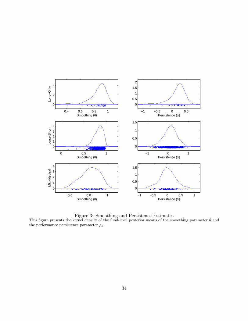
In this subsection we give a graphical representation of the estimates of the most complete
model (Figure 3)and compare the smoothing, persistence, and shrinkage parameter estimates
of the eight possible models (Table 7). In Figure 3 we present the funds’ posterior means
of the smoothing and performance persistence parameters. As can be seen, most of the
estimates of θ lie between 0.5 and 1 across all 3 strategies. Theoretically, if smoothing
is intentional, a fund manager that wants to maximize his reported Sharpe ratio would
not smooth beyond one half the fund’s current realized returns since the observed returns
variance is minimized at θ = 0.5. The location of the smoothing parameters is between 0.8
and 0.9 and is highest for the long-only strategy, and lowest for the market-neutral strategy.
This finding is consistent with the belief that the latter strategy is less liquid than the former
since it might make a greater use of derivatives, which might be characterized by stale prices.
With regard to abnormal performance, we find that it displays various levels of persis-
tence across the three investment categories. Figure 3 shows that most of the performance
persistence parameters range from approximately -0.1 to +0.5 for the long-only strategy,
and between -0.5 and +0.5 for the long-short and market-neutral strategies. This finding
offers new insights on performance persistence studies which are typically implemented by
estimating a model with constant α over different consecutive samples. We improve on this
paradoxical approach by making persistence part of the estimation, and find that for many
funds positive performance is more likely to be followed by negative performance. Notice
that our framework lends itself to be used as a model of expected abnormal performance
which could be used to implement fund-of-funds trading strategies, but this is beyond the
12

scope of the present study which focuses on performance evaluation. We leave this important
issue for future research.
The density plots shown so far only give information on the means of posterior distribu-
tions. In Table 7 we provide information on both the location and the scale of the posterior
distributions of θ and ρα for the eight estimated models (the mdoels are ordered as in Table
2). Notice that for models that do not account for a specific feature of observed retruns (e.g.
smoothing), the posterior parameters is set equal to the corresponding implicit restriction
(e.g. equal to one for smoothing). As can be seen, the posterior mean (and median)of the
smoothing parameter θ is consistent across the 8 models and is slightly decreasing from
the long-only strategy going to the market-neutral strategy. Most importantly, the column
Pct > 0 indicates that our estimates are also significant. This column reports the propor-
tion of funds whose smoothing estimates is at least two standard deviation away from the
value of one, which represents the null hypothesis of no-smoothing. The table therefore
shows (considering model1) that more than 60% of the 937 equity funds are characterized
by statistically significant smoothing. We will show that this smoothing is also economically
relevant.
The correct null hypothesis for ρα is that it is equal to zero (lack performance persis-
tence/autocorrelation). As can be seen, the proportion of significant ραs is far smaller than
that obtained for θ, and is decreasing over fund strategies (going from Panel A to Panel
B, considering model 1). Interestingly, this proportion increases for model 6, reaching ap-
proximately 40%, which only accounts for funds dynamics. The lower significance of the
persistence parameter is probably due to the lack of information, since a lot of time series
observations are likely needed to appropriately asses the dynamics of a single fund.
Finally the last three columns of Table 7 show a moderate amount of shrinkage of the
individual funds’ α and β′s toward their strategy counterparts. The shrinkage can be better
appreciated by looking at Figure 4, which reports a density plot of the funds’ long-run alpha
and betas (α and β′s) across the three equity strategies considered in the paper. Figure 4
also reveals the essentially unimodal nature of the distribution, and a lower shrinkage for
the long-only strategy. With regard to the actual location of the distribution, we see that
hedge funds do deliver α in the long run, but they also bear more risk than what is usually
perceived. Even for the market-neutral equity strategy, we see that the distribution of the
13
posterior means of the market beta is skewed to the right indicating a sensitivity to market
movements.
5.2.2 Impact of Smoothing on Measured Risk and Performance
In this section we report several statistics on the regression parameters estimated with both
OLS and Bayesian methods. Table 8 compares OLS and Bayesian estimates under the as-
sumption of no smoothing (θ = 1). For each strategy, we report the sample mean, standard
deviation, and several percentiles of the distribution of the estimated coefficients. The results
are categorized by investment strategy. In addition to the α and β coefficients, for complete-
ness, the last column also reports the estimated Bayesian standard deviation of the shocks.
As can be seen, udner the assumption of no smoothing, the OLS estimates and posterior
means of the Bayesian estimates are virtually identical. This similarity in the estimates given
by the two methods is to be expected, given the diffuseness of the priors. This similarity
also indicates that our estimates under the assumption of smoothing are not driven by the
use of Byesian methods.
Table 9 reports OLS and Bayesian estimates under the assumption of smoothing (θ ∈[0, 1]). In the first three columns the OLS estimates are obtained by regressing the hedge
funds’ returns on current and lagged factors and summing the two betas relative to each
factor. This OLS approach, proposed by Asness, Krail, and Liew (2001), provides an ap-
proximate way of dealing with smoothing. The remaining columns of the tables report
average (by strategy) of the posterior means of the alphas, betas, standard deviations, and
smoothing parameters. Both the OLS and Bayesian approach give substantially higher betas
than those obtained under the assumption no-smoothing indicating that smoothing induces
a downward bias in the estimated risk exposures.10 The estimated alphas are also typically
lower when we account for smoothing, but the difference is in the scale of basis points and
less easy to detect from the table.
In addition to the numerical evidence reported in the tables, we provide graphical evidence
on the extent of smoothing and its impact on performance evaluation. Figure 5 presents a
box plot with the distribution of the estimated parameter θ for the three equity strategy
10Note that if the true loading are negative, then smoothing actually induces an upward bias in the betas,and a downward bias in the alphas.
14

considered in this subsection (model5). The boxplots, and Table 9, indicate that the median
smoothing is between 0.90, 0.86, and 0.75 for the Long Only, Long/Short, and Market
Neutral equity groups respectively. We postulate that equity hedge funds are among those
funds less affected by smoothing, and, therefore, 0.90 can be considered an upper bound on
the median θ that we can expect to find in other strategy groups. Hence, we are inclined to
state that smoothing is pervasive phenomenon in the hedge fund industry.
Next, we asses the impact of smoothing on performance evaluation. In Figure 6, we
present scatter plots of the difference between the standard OLS (from model 1) and the
Bayesian estimates of α and the βs (from model 5) against smoothing (θ). In the construction
of the scatter plots (and the fitted line), we drop funds with an estimated θ in excess of the
20th percentile of the strategy group to which it belongs. Furthermore, to reduce the influence
of outliers, the fitted lines are fit to the data after eliminating observations with a studentized
residual in excess of 3. With regard to the effect on abnormal performance, the plots show
that the decrease in alpha going from θ = 1 to the lowest θ in the range is approximately 10
basis point, which is equivalent to an annualized abnormal performance difference of 1.21%.
More precisely, a standard deviation change in θ generates a bias of approximately 5, 2,
and 1 basis points for the first, second, and third strategy respectively. This shows that
smoothing has an economic impact as well as statistical.11
Like abnormal performance, a correct assessment of the funds’ risk exposures is an im-
portant aspect of the investment decision process. With regard to the loading on the market
factor, Figure 6 shows that accounting for smoothing yields substantially higher estimates of
the factor loading, with the discrepancy in beta going from approximately zero up to 0.20 as
θ decreases. The same pattern emerges for the loading on the size spread factor. Probably,
the effect of smoothing is less strong for this factor, reflecting the fact that the size spread
factor accounts for less variation in hedge funds’ returns than does the market factor.
6 Conclusion
When the underlying real hedge fund returns are smoothed, due either to illiquidity or out-
right fraudulent behavior, this smoothing can lead to biases in performance evaluation studies
11The economic significance is obtained by multiplying the standard deviation of θ by the slope coefficient.
15

which are both statistically and economically significant. In the cases that we considered, i.e.
equity hedge funds, we find that, even for these relatively liquid strategies, smoothing causes
an upward bias in excess performance measures, e.g. the fund’s α, and a downward bias in
risk measures. In particular, we show that a moderate level of smoothing can cause the stan-
dard OLS α to over-estimate equity funds’ abnormal performance by more than 1% annually.
In addition, we find that ignoring the dynamic aspect of hedge funds’ trading strategies, and
the similarity of hedge funds in a given category, is potentially important. However, these
effects are dwarfed by the effect of ignoring return smoothing. Finally, we anticipate that
the findings from this paper represent a lower bound of the impact of smoothing on hedge
fund performance evaluation for the rest of the hedge fund industry as we expect the effect
of smoothing to be more pronounced for more illiquid investment strategies because of the
discretion and difficulty that managers have in marking to market their positions.
16

A Appendix
A.1 Simulation example: unconditional CAPM
This example is based on the unconditional CAPM model and shows what can go wrong if
we ignore return smoothing. Consider what happens when reported returns are a weighted
average of current and past true economic returns. Excess returns for fund i at time t are
generated by the model
yit = αi + β′ixt + εit,
where yit is the fund’s excess return and xt is the excess return on the market. The parameters
βi and αi represent systematic risk and abnormal performance respectively. We generate
returns for 2000 funds and set T = 60 for all of them. We set αi = 0 for all funds and draw
the βi from a uniform distribution with support equal to [0, 2]. For each fund we draw the
return smoother θ from a uniform distribution so that some funds smooth returns more than
other. We regress yot = θiyt + (1 − θi)yt−1 on a constant and xt using OLS. We report the
bias for both estimated parameters as a function of θ.
As shown by Figure 1 return smoothing inflates estimated measures of risk-adjusted
performance (α) while deflating estimated measures of risk (β).
A.2 Posterior Distributions: base case (θ = 1)
(i) p(β|β, σ2, ρ∆, DT ): using the likelihood in (4) and the prior in (18), we have
p(β|β, σ2ε , ρ, ∆, DT ) ∼ N(Xβ, σ2
εIT )×N(A1β, A2(IT ⊗∆)A′2)
∼ N(B, V ), (20)
where,
B = V × (X ′Y/σ2
ε + A2(IT ⊗∆)A′2)−1A1β
)
V =(X ′X/σ2
ε + A2(IT ⊗∆)A′2)−1
)−1.
(ii) p(β|β, Σ, ∆, ρ, DT ): plug expression (18) into (3) to get
Y = XA1β + XA1η + ε
Y = X∗β + ε∗, ε∗ ∼ N(0, Q),
17

where Q = [σ2εIT + XA2(IT ⊗∆)A′
2X′]. Using the prior for β, we have
p(β|β, Σ, ∆, ρ, DT ) ∝ exp
−1
2(β − βStr)
′Σ−1(β − βStr)
× exp
−1
2(Y −X∗β)′Q−1(Y −X∗β)
∝ N(B, V ), (21)
where, B = V × (Σ−1βStr + X∗′Q−1Y ) and V = (Σ−1 + X∗′Q−1X∗)−1.
(iii) p(σ2ε |β, DT ): using the IG prior for σ2
ε , we have
p(σ2ε |β,DT ) ∼ p(σ2
ε |β)× p(Y |X, β, σ2ε)
∝(
1
σ2ε
)sh+1+T2
exp−sc/σ2
ε − (Y −Xβ)′(Y −Xβ)/2σ2ε
∼ IG(T/2 + sc, SSR/2 + sc), (22)
where SSR ≡ (Y −Xβ)′(Y −Xβ).
(iv) p(Σ|βi ∈ stratj): using the IG prior for Σ, we have
p(Σ|βi ∈ stratj) ∼ p(Σ|sh, sc)×∏
i∈stratj
p(βi|βStr, Σ)
∝K∏
k=1
(1
σ2k
)sh+1+nj2
exp
−
sc
σ2k
−∑
i∈stratj
(βk − βStr,k)2
2σ2k
, (23)
where βk and βStr,k are the kth elements of the vectors β and βStr respectively. The kernel
in (23) factors in several independent kernels for each δk:
p(σ2k|βi ∈ stratj) ∼ IG(nj/2 + sh, SSRσk
/2 + sc), k = 1, . . . , K, (24)
where the definition of SSRδkis obvious.
(v) p(∆|β, β1, . . . , βT , ρ): the information for this posterior density is contained in (11)
and (14). Therefore, denoting the demeaned β with β∗,
p(∆|β, β) ∝ p(∆)× p(β1, . . . , βT |∆)
∝K∏
k=1
(1
δ2k
)sh+1+T2
exp
−sc/δ2
k −T∑
t=1
(β∗kt − ρkβ∗kt−1)
2/2δ2k
, (25)
18

where β∗kt refers the kth element of the vector β∗t . The kernel in (25) factors in several
independent kernels for each δk:
p(δ2k|βk, βk, ρk) ∼ IG(T/2 + sh, SSRδk
/2 + sc), k = 1, . . . , K, (26)
where the definition of SSRδkis obvious.
(vi) p(ρk|β, β, ∆): Using independence of the elements of ρ, we have
p(ρk|β, β, ∆) ∝ TN(−1,1)(0, σ2ρ,k)×
T∏t=1
N(ρβ∗k,t−1, δ2k)
∝ TN(−1,1)(ρk, σρk), k = 1, . . . , K, (27)
where ρk = σρk×∑T
t=1 β∗k,tβ∗k,t−1 and σρk
= 1/(1/σ2k +
∑Tt=1 β∗2k,t−1/δ
2k).
A.3 Posterior Distributions: general case (θ ∈ [0, 1])
(i) p(β|β, σ2ε , ∆, ρ, θ, DT ): using the likelihood in (10) and the prior in (18), we have
p(β|β, σ2ε ∆, θ,DT ) ∼ N(B, V ), (28)
where,
B = V × (Xo′Ω−1Y o/σ2
ε + (A2(IT ⊗∆)A′2)−1A1β)
)
V =(Xo′Ω−1Xo/σ2
ε + (A2(IT ⊗∆)A′2)−1
)−1.
(ii) p(β|σ2ε , ∆, ρ, θ, DT , ): the only difference is in the matrix Q and the sample size
(shorter by one observation). Plug expression (18) into (9) to get
Y o = XoA1β + XoA2η + ε
= X∗1 β + ε∗, ε∗ ∼ N(0, Q),
where now we have Q = [σ2εΩ + XoA2(IT ⊗∆)A′
2Xo′]. The rest of the derivation is just like
the base case.
(iii) p(σ2ε |β, θ, DT ): with a prior for σ2
ε given by (16), we have
p(σ2ε |β, θ, DT ) ∼ p(σ2
ε |β)× p(Y o|Xo, β, σ2ε)
∝(
1
σ2ε
)sh+1+T2
exp−sc/σ2
ε − (Y o −Xoβ)′Ω−1(Y o −Xoβ)/2σ2ε
∼ IG(T o/2 + sh, SSR/2 + sc), (29)
19

where now SSR ≡ (Y o −Xoβ)′Ω−1(Y o −Xoβ).
(iv) p(Σ|βi ∈ stratj): same as base case.
(v) p(∆|β1, . . . , βT ): same as base case.
(vi) p(ρk|β, β, ∆): same as base case.
(vii) p(θ|β, σ2ε , DT ): Combining the likelihood in (10) with the prior for θ, we have
p(θ|β, σ2ε , DT ) ∼ Beta(a, b)×N(Xoβ, σ2
εΣ)
∝ θa−1(1− θ)b−1
|Ω|1/2exp
−(Y o −Xoβ)′Ω−1(Y o −Xoβ)
2σ2ε
(30)
This posterior distribution is not a standard one and a Metropolis-Hastings algorithm is
required to sample from it.
20

References
Asness, C. S., Krail, R., Liew, J. M., 2001. Do Hedge Funds Hedge?. SSRN eLibrary.
Bollen, N. P., Pool, V. K., 2006. A Screen for Fraudulent Return Smoothing in the Hedge
Fund Industry. SSRN eLibrary.
Bollen, N. P., Whaley, R. E., 2007. Hedge Fund Risk Dynamics: Implications for Performance
Appraisal. SSRN eLibrary.
Busse, J. A., Irvine, P. J., 2006. Bayesian alphas and mutual fund persistence. The Journal
of Finance 61(5), 2251–2288.
Ferson, W. E., Harvey, C. R., 1991. The variation of economic risk premiums. The Journal
of Political Economy 99(2), 385–415.
Ferson, W. E., Schadt, R. W., 1996. Measuring fund strategy and performance in changing
economic conditions. The Journal of Finance 51(2), 425–461.
Fung, W., Hsieh, D. A., 2000. Performance characteristics of hedge funds and commodity
funds: Natural vs. spurious biases. The Journal of Financial and Quantitative Analysis
35(3), 291–307.
, 2004. Hedge fund benchmarks: A risk-based approach. Financial Analysts Journal
60(5), 65–81.
Getmansky, M., Lo, A. W., Makarov, I., 2004. An econometric model of serial correlation
and illiquidity in hedge fund returns. Journal of Financial Economics 74(3), 529–609.
Kosowski, R., Naik, N. Y., Teo, M., 2007. Do hedge funds deliver alpha? a bayesian and
bootstrap analysis. Journal of Financial Economics 84(1), 229–264.
Liang, B., 2000. Hedge funds: The living and the dead. The Journal of Financial and Quan-
titative Analysis 35(3), 309–326.
Lopes, H., West, M., 2004. Bayesian Model Assessment in Factor Analysis. Statistica Science
14, 41–67.
21

Mamaysky, H., Spiegel, M., Zhang, H., 2007. Estimating the Dynamics of Mutual Fund
Alphas and Betas. Review of Financial Studies.
Newton, M., Raftery, A., 1994. Approximate Bayesian inference with weighted likelihood
bootstrap. Journal of the Royal Statistical Society 56, 3–48.
Pastor, L., Stambaugh, R. F., 2002. Mutual fund performance and seemingly unrelated
assets. Journal of Financial Economics 63(3), 315–349.
Pool, V. K., Bollen, N. P., 2007. Do Hedge Fund Managers Misreport Returns? Evidence
from the Pooled Distribution. SSRN eLibrary.
Weisman, A. B., 2002. Informationless investing and hedge fund performance measurement
bias.. Journal of Portfolio Management 28(4), 80–91.
22

Table 1: Simulation: Data Generating Process
This table reports the parameters used in the data gener-ating process in the simulation study.
Parameters:βOLS = [0, 1] σε = 0.012 θ ∼ Uni[0, 1]∆ = [0.012 0.12] Σ = [0.012 0.12] Σρ = [1 0.1]xt ∼ N(0.01, 0.15)Simulation Set Up:1 strategy (J = 1) 100 funds (I = 100)1 factor (K = 1) Ti ∼ Uni[30, 144]
23

Table 2: Simulation: Model Comparison
This table presents statistics on the fitting of funds’ estimates of α and β. The first four column identify themodel under investigations. A one indicate that the smoothing, dynamic, or shrinkage feature is retainedand a zero indicates otherwise. Bias(·) is the average difference between the estimated and true parametersfor all funds. MAD(·) is the mean absolute deviation. RMSE(·) is the root mean squared error of theestimates. The last column reports the posterior probability, given the priors and the likelihood, of theestimated models.
Sm Dy Sr Bias(α) MAD(α) RMSE(α) Bias(β) MAD(β) RMSE(β) Post. Pr.
1 1 1 1 0.000 0.008 0.011 -0.000 0.062 0.081 1.0002 1 1 0 0.000 0.009 0.011 -0.000 0.063 0.082 0.0003 1 0 1 0.000 0.014 0.018 -0.005 0.092 0.116 0.0004 0 1 1 0.000 0.031 0.047 -0.488 0.494 0.595 0.0005 1 0 0 0.000 0.014 0.018 -0.005 0.092 0.117 0.0006 0 1 0 0.000 0.046 0.067 -0.521 0.527 0.639 0.0007 0 0 1 0.000 0.015 0.019 -0.477 0.484 0.574 0.0008 0 0 0 0.000 0.015 0.019 -0.486 0.493 0.586 0.000
24

Table 3: Hedge Fund Strategies
This table presents the fund categories (strategies) considered in the analysis. Each strategy is assigned acode which will be used in the remainder of the paper. The third column reports the number of funds ineach category. The remaining three columns report the sample size of the fund with the lowest, median, andmaximum number of observations within each category.
ObservationsCode Category N. Funds Min Median Max
1 Capital Structure Arbitrage 4 46 53.5 842 Convertible Arbitrage 102 30 58 1443 Distressed Securities 77 31 56 1444 Emerging Markets 183 30 63 1445 Equity Long Only 40 30 60 1446 Equity Long/Short 834 30 60 1447 Equity Market Neutral 96 30 54 1448 Event Driven Multi Strategy 90 30 74.5 1449 Fixed Income 21 34 58 144
10 Fixed Income - MBS 33 32 74 11211 Fixed Income Arbitrage 56 31 45 10212 Global Macro 101 30 60 14413 Market Timing 5 75 81 10514 Merger Arbitrage 66 33 63 14415 Multi Strategy 28 34 64 14416 Option Arbitrage 7 37 47 10817 Other Relative Value 3 91 111 12018 Regulation D 4 80 86 11519 Relative Value Multi Strategy 40 30 66.5 14220 Sector 179 30 60 14421 Short Bias 31 33 64 144
All 2000 30 60 144
25

Table 4: Hedge Fund Descriptive Statistics
This table presents descriptive statistics on monthly returns reported by hedge funds in the CISDM database. The first column reports the codes associated to each strategy (see Table 1). The second and thirdcolumn report the smallest and largest monthly reported return in each strategy. The last four columnsreport the strategy average of the mean, standard deviation, skewness, and kurtosis of hedge fund returns.
Code Min Max Mean SD SK KUR
1 -0.039 0.162 0.015 0.021 1.581 5.3782 -0.410 0.520 0.008 0.025 -0.192 2.9053 -0.583 0.610 0.011 0.034 0.088 3.6644 -1.000 2.257 0.012 0.069 -0.290 4.5675 -0.549 0.835 0.009 0.063 -0.233 1.2356 -1.000 1.225 0.010 0.051 0.178 2.6797 -0.820 0.362 0.006 0.025 -0.153 2.7888 -0.543 0.885 0.011 0.033 -0.152 3.5309 -0.201 0.212 0.006 0.025 -0.760 3.515
10 -0.357 0.322 0.009 0.025 -2.059 17.17511 -0.528 0.249 0.004 0.024 -1.020 7.26612 -0.518 0.742 0.008 0.048 0.282 3.47813 -0.144 0.262 0.010 0.033 0.524 2.38314 -0.320 1.842 0.006 0.021 -0.310 4.17815 -0.215 0.408 0.008 0.027 0.250 2.79616 -0.120 0.238 0.005 0.032 0.988 3.77317 -0.068 0.145 0.009 0.025 0.671 3.98218 -0.108 0.214 0.008 0.020 0.993 5.73519 -0.192 0.617 0.009 0.017 -0.017 6.14920 -0.483 0.909 0.012 0.067 0.363 3.42321 -0.574 0.660 0.003 0.070 0.183 2.143All -1.000 2.257 0.010 0.047 0.005 3.528
26

Table 5: Seven Factors Descriptive Statistics
This table presents descriptive statistic on the seven factors. The first three factors are bond, currency, andcommodity trend-following risk factors respectively. They are constructed by Fung and Hsieh (2004) andare available at http://faculty.fuqua.duke.edu/~dah7/DataLibrary/TF-FAC.xls. The equity marketfactor is the Standard & Poors 500 index monthly total return. The size spread factors is the monthly returnon the Russell 2000 index minus the monthly return on the Standard & Poors 500. The bond market factoris the monthly change in the 10-year treasury constant maturity yield. The Credit Spread Factor is themonthly change in the Moody’s Baa yield minus the 10-year treasury constant maturity yield.
Factors Min Max Mean SD SK KUR ρ
Equity Market -0.147 0.094 0.006 0.043 -0.577 3.549 -0.015Size Spread -0.164 0.183 -0.000 0.038 0.258 7.421 -0.133Bond Market -0.005 0.006 -0.000 0.002 0.389 2.727 0.249Credit Spread -0.003 0.005 -0.000 0.001 0.918 5.022 0.372Bond Trend -0.254 0.689 -0.005 0.152 1.507 6.153 0.094Currency Trend -0.301 0.903 -0.002 0.191 1.339 6.029 0.010Commodity Trend -0.229 0.648 -0.008 0.130 1.466 7.141 -0.142
27

Table 6: Variable Selection and Unconditional Models’ Fit
This table presents selection and estimation results of the variable selection criterion based on R2. For each ofthe 937 equity funds, we estimate 27 regression models using all the possible combinations available with sevenfactors. We then divide these regressions into seven groups depending on the number of included factors,and rank them according to their R2. Finally, we retain, for every fund and every group, the regressionwith the highest R2. Panel A reports the number of times each factor is selected by our procedure. Panel Breports average estimates of α and β, and average R2s.
Factors α β1 β2 β3 β4 β5 β6 β7 R2
PANEL A: selected factors
1 937 539 216 38 49 23 31 412 937 704 547 143 149 119 88 1243 937 767 651 293 329 295 191 2854 937 821 731 468 504 449 335 4405 937 865 810 617 666 618 516 5936 937 906 871 781 807 770 703 7847 937 937 937 937 937 937 937 937
PANEL B: estimates and fit
1 0.005 0.573 0.471 -1.357 -12.024 -0.005 0.027 0.048 0.2492 0.004 0.526 0.431 -1.017 -7.101 -0.006 0.029 0.037 0.3343 0.004 0.498 0.383 -1.223 -5.666 -0.006 0.027 0.034 0.3644 0.004 0.467 0.352 -1.000 -4.185 -0.006 0.019 0.029 0.3795 0.004 0.444 0.322 -0.890 -3.311 -0.006 0.014 0.021 0.3876 0.004 0.423 0.302 -0.792 -2.838 -0.006 0.011 0.016 0.3917 0.004 0.409 0.280 -0.666 -2.432 -0.006 0.008 0.014 0.392
28

Table 7: Model Comparison
This table presents the average and the median of the funds’posterior means of θ and ρα and, the average ofthe posterior mean of the shrinkage estimates. The column Pct < 1 reports the proportion of the smoothingestimates that are at least two standard deviations away from the value of one. The column Pct ≷ 0 reportsthe proportion of the persistence estimates that are at least two standard deviations away from the valueof zero. The results are reported for each of the 8 models considered in the study, and are categorized byinvestment strategy. Fields corresponding to model restrictions report values implied by the restriction. Forinstance, the fields for model8 are not estimates. These fields simply indicate the restrictions we use toestimate a model with no smoothing, no dynamics, and no shrinkage.
θ ρα Σ
Mean Median Pct < 1 Mean Median Pct ≷ 0 α β1 β2
PANEL A: Equity Long Only
1 0.862 0.886 0.538 0.177 0.233 0.077 0.005 0.514 0.2422 0.846 0.863 0.590 0.250 0.311 0.128 1000 1000 10003 0.889 0.921 0.359 0.000 0.000 0.000 0.005 0.588 0.2824 1.000 1.000 0.000 0.317 0.339 0.103 0.005 0.442 0.1935 0.898 0.916 0.333 0.000 0.000 0.000 1000 1000 10006 1.000 1.000 0.000 0.407 0.432 0.282 1000 1000 10007 1.000 1.000 0.000 0.000 0.000 0.000 0.006 0.506 0.2208 1.000 1.000 0.000 0.000 0.000 0.000 1000 1000 1000
PANEL B: Equity Long/Short
1 0.824 0.839 0.654 0.090 0.107 0.108 0.003 0.506 0.3092 0.811 0.821 0.738 0.252 0.294 0.151 1000 1000 10003 0.799 0.879 0.397 0.000 0.000 0.000 0.003 0.528 0.3664 1.000 1.000 0.000 0.338 0.330 0.204 0.003 0.390 0.2555 0.806 0.874 0.421 0.000 0.000 0.000 1000 1000 10006 1.000 1.000 0.000 0.436 0.442 0.300 1000 1000 10007 1.000 1.000 0.000 0.000 0.000 0.000 0.004 0.410 0.2948 1.000 1.000 0.000 0.000 0.000 0.000 1000 1000 1000
PANEL C: Equity Market Neutral
1 0.815 0.827 0.621 0.009 -0.009 0.074 0.003 0.230 0.0642 0.779 0.778 0.768 0.192 0.220 0.042 1000 1000 10003 0.745 0.860 0.253 0.000 0.000 0.000 0.003 0.256 0.1074 1.000 1.000 0.000 0.300 0.299 0.147 0.003 0.184 0.0845 0.742 0.845 0.305 0.000 0.000 0.000 1000 1000 10006 1.000 1.000 0.000 0.400 0.405 0.211 1000 1000 10007 1.000 1.000 0.000 0.000 0.000 0.000 0.004 0.229 0.1158 1.000 1.000 0.000 0.000 0.000 0.000 1000 1000 1000
29

Table 8: Individual Estimates: No Smoothing (model8)
This table presents the sample mean (Mean), standard deviation( SD) and percentiles (5th pct, and 95th pct)of the estimated OLS and bayesian parameters. The results are categorized by investment strategy. Inaddition to the α and β coefficients, the last column also report the estimated Bayesian standard deviationof the shocks.
OLS BAYES
α β1 β2 α β1 β2 σε
PANEL A: Equity Long Only
Mean 0.004 0.713 0.292 0.004 0.714 0.293 0.042St. Dev 0.009 0.565 0.322 0.009 0.564 0.326 0.027Min -0.019 -0.585 -0.432 -0.019 -0.586 -0.421 0.0115th -0.007 -0.446 -0.190 -0.007 -0.443 -0.191 0.01150th pct 0.003 0.762 0.266 0.003 0.762 0.267 0.03395th pct 0.022 1.769 0.882 0.022 1.758 0.878 0.103Max 0.028 2.008 1.068 0.028 2.007 1.118 0.110
PANEL B: Equity Long/Short
Mean 0.004 0.428 0.322 0.004 0.427 0.322 0.038St. Dev 0.008 0.485 0.386 0.008 0.485 0.386 0.022Min -0.040 -2.534 -0.928 -0.038 -2.550 -0.934 0.0075th pct -0.009 -0.183 -0.125 -0.009 -0.183 -0.123 0.01250th pct 0.005 0.351 0.246 0.005 0.352 0.247 0.03395th pct 0.016 1.371 1.050 0.016 1.369 1.033 0.078Max 0.035 2.957 3.288 0.035 2.943 3.288 0.167
PANEL C: Equity Market Neutral
Mean 0.003 0.064 0.070 0.003 0.063 0.069 0.023St. Dev 0.005 0.306 0.177 0.005 0.306 0.177 0.014Min -0.005 -0.927 -0.286 -0.005 -0.934 -0.286 0.0075tht -0.003 -0.275 -0.173 -0.003 -0.274 -0.172 0.00850th pct 0.002 0.036 0.030 0.002 0.037 0.031 0.02095th pct 0.014 0.492 0.406 0.014 0.492 0.407 0.056Max 0.025 1.777 0.570 0.025 1.780 0.570 0.079
30

Table 9: Individual Estimates: Smoothing (model5)
This table presents the sample mean (Mean), standard deviation( SD) and percentiles (5th pct, and 95th pct)of the estimated OLS and bayesian parameters. The results are categorized by investment strategy. Inaddition to the α and β coefficients, the last two columns also report the Bayesian estimates of the standarddeviation of the shocks and of the smoothing parameter.
OLS BAYES
α β1 β2 α β1 β2 σε θ
PANEL A: Equity Long Only
Mean 0.003 1.005 0.075 0.003 0.802 0.293 0.048 0.898St. Dev 0.009 0.780 0.273 0.008 0.621 0.337 0.032 0.059Min pct -0.032 -0.564 -0.468 -0.016 -0.611 -0.500 0.013 0.7135th -0.007 -0.416 -0.369 -0.007 -0.454 -0.198 0.013 0.77850th pct 0.003 0.980 0.059 0.003 0.892 0.265 0.036 0.91695th pct 0.018 2.398 0.578 0.019 1.923 0.920 0.117 0.960Max 0.023 3.095 1.019 0.026 2.368 1.065 0.140 0.968
PANEL B: Equity Long/Short
Mean 0.004 0.743 0.158 0.004 0.498 0.361 0.043 0.806St. Dev 0.009 0.770 0.287 0.009 0.545 0.441 0.025 0.193Min -0.053 -3.172 -0.914 -0.049 -2.877 -1.020 0.007 0.0725th pct -0.009 -0.155 -0.180 -0.010 -0.183 -0.173 0.015 0.28050th pct 0.004 0.618 0.128 0.004 0.421 0.281 0.037 0.87495th pct 0.015 2.215 0.587 0.016 1.513 1.210 0.090 0.955Max 0.039 5.868 2.414 0.035 3.516 3.569 0.206 0.977
PANEL C: Equity Market Neutral
Mean 0.003 0.127 0.033 0.003 0.089 0.072 0.026 0.742St. Dev 0.005 0.367 0.145 0.005 0.345 0.188 0.016 0.249Min -0.006 -0.689 -0.355 -0.005 -1.009 -0.353 0.008 0.0805th pct -0.003 -0.234 -0.185 -0.003 -0.287 -0.175 0.010 0.12750th pct 0.002 0.042 0.016 0.002 0.048 0.037 0.023 0.84595th pct 0.012 0.808 0.324 0.013 0.608 0.408 0.062 0.956Max 0.029 2.038 0.609 0.026 1.860 0.613 0.087 0.986
31

0 0.2 0.4 0.6 0.8 1−0.02
0
0.02
0.04
Theta
Alp
ha B
ias
0 0.2 0.4 0.6 0.8 1−3
−2
−1
0
1
Bet
a B
ias
Theta
Figure 1: Smoothing Bias
Excess returns for fund i at time t are generated by the model yit = αi + βi′xt + εit, where yit is the fund’sexcess return and xt is the excess return on the market. The parameters βi and αi represent systematic riskand abnormal performance respectively. We generate returns for 2000 funds and set T = 60 for all of them.We set αi = 0 for all funds and draw the βi from a uniform distribution with support equal to [0, 2]. Foreach fund we draw the return smoother θ from a uniform distribution so that some funds smooth returnsmore than other. We regress yo
t = θiyt + (1 − θi)yt−1 on a constant and xt using OLS. We report the biasfor both estimated parameters as a function of θ.
32

Figure 2: Distribution of Hedge Funds’ Sample SizeThis figure presents the distribution of hedge funds’ life-spans, measured in months, in our sample.
33
0.4 0.6 0.8 1
0
2
4
Long
−O
nly
Smoothing (θ)−1 −0.5 0 0.5
0
0.5
1
1.5
2
Persistence (α)
0 0.5 1
0
1
2
3
4
Long
−S
hort
Smoothing (θ)−1 0 1
0
0.5
1
1.5
Persistence (α)
0.6 0.8 1
0
1
2
3
4
Mkt
−N
eutr
al
Smoothing (θ)−1 −0.5 0 0.5 1
0
0.5
1
1.5
Persistence (α)
Figure 3: Smoothing and Persistence EstimatesThis figure presents the kernel density of the fund-level posterior means of the smoothing parameter θ andthe performance persistence parameter ρα.
34

0 50 100
0
5
10
15
20x 10
−3
Long
−O
nly
Performance0 1 2
0
0.5
1
Mkt Beta−0.2 0 0.2 0.4 0.6 0.8
0
1
2
Size Sprd Beta
0 50 100
0
0.01
0.02
0.03
Long
−S
hort
Performance−2 0 2
0
0.5
1
Mkt Beta−0.5 0 0.5 1 1.5
0
0.5
1
1.5
2
Size Sprd Beta
0 50 100
0
0.01
0.02
Mkt
−N
eutr
al
Performance−0.5 0 0.5 1
0
1
2
3
Mkt Beta−0.1 0 0.1
0
5
10
Size Sprd Beta
Figure 4: Long-run Coefficients and ShrinkageThis figure presents the kernel density of the fund-level posterior means of α and β′s (long-run abnormalperformance and factor loadings). Abnormal performance is measured in basis points.
35

Long Only Long/Short Market Neutral
0.1
0.2
0.3
0.4
0.5
0.6
0.7
0.8
0.9
1
Sm
ooth
ing
(θ)
Equity Strategies
Figure 5: Smoothing by StrategyThis figure presents the distribution, by investment strategy, of the estimated smoothing parameters θ.
36

0.85 0.9 0.95 1−40
−20
0
20
40
αBay
es−
αOls
Long Only
β =161.44 (1.73)
σ(θ)=0.03
0.85 0.9 0.95 10
0.05
0.1
0.15
0.2
β 1Bay
es−
β 1Ols
Long Only
β =−1.05 (−3.26)
σ(θ)=0.03
0.85 0.9 0.95 1−0.1
0
0.1
0.2
0.3
β 2Bay
es−
β 2Ols
Long Only
β =−0.04 (−0.11)
σ(θ)=0.03
0.7 0.8 0.9 1−40
−20
0
20
40
αBay
es−
αOls
Long/Short
β =38.76 (4.62)
σ(θ)=0.05
0.7 0.8 0.9 1−0.2
0
0.2
0.4
0.6
β 1Bay
es−
β 1Ols
Long/Short
β =−0.49 (−8.59)
σ(θ)=0.05
0.7 0.8 0.9 1−0.2
0
0.2
0.4
0.6
β 2Bay
es−
β 2Ols
Long/Short
β =−0.15 (−3.08)
σ(θ)=0.05
0.4 0.6 0.8 1−20
−10
0
10
αBay
es−
αOls
Market Neutral
Smoothing (θ)
β =8.66 (0.74)
σ(θ)=0.11
0.4 0.6 0.8 1−0.1
0
0.1
0.2
0.3
β 1Bay
es−
β 1Ols
Market Neutral
Smoothing (θ)
β =−0.32 (−2.90)
σ(θ)=0.11
0.4 0.6 0.8 1−0.05
0
0.05
0.1
0.15
β 2Bay
es−
β 2Ols
Market Neutral
Smoothing (θ)
β =−0.11 (−2.37)
σ(θ)=0.11
Figure 6: Bias Vs SmoothingThis figure presents scatter plots, by investment strategy, of the difference between OLS and Bayesian alphasand betas. The scale on the alpha graphs is expressed in basis points. The graphs report observations forwhich θ is above the 25th percentile of the strategy group and for which the funds loadings are both positive.To reduce the influence of outliers, the fitted lines are fit to the data after eliminating observations with astudentized residual in excess of 3, and a Cook’s distance ten times bigger than the median Cook’s distancein the strategy group.
37


