

SOME PERTURBATION METHODS TO SOLVE LINEARAND NON-LINEAR DIFFERENTIAL EQUATION
A PROJECT REPORT
submitted by
SASHI KANTA SAHOO
Roll No: 412MA2079
for
the partial fulfilment for the award of the degree
of
Master of Science in Mathematics
under the supervision
of
Dr. BATA KRUSHNA OJHA
DEPARTMENT OF MATHEMATICS
NATIONAL INSTITUTE OF TECHNOLOGY
ROURKELA– 769008
MAY 2014

Declaration
I declare that the topic “SOME PERTURBATION METHODS TO SOLVE LIN-
EAR AND NON-LINEAR DIFFERENTIAL EQUATION ” for completion for
my master degree has not been submitted in any other institution or university for the
award of any other degree or diploma.
Date: May 2014
Place: NIT, Rourkela(Sashi Kanta Sahoo)
Roll no: 412MA2079
Department of Mathematics
NIT Rourkela
1

Certificate
This is to certify that the project report entitled SOME PERTURBATION METH-
ODS TO SOLVE LINEAR AND NON-LINEAR DIFFERENTIAL EQUA-
TION submitted by Sashi Kanta Sahoo to the National Institute of Technology
Rourkela, Odisha for the partial fulfilment of requirements for the degree of master of
science in Mathematics and the review work is carried out by him under my supervision
and guidance. It has fulfilled all the guidelines required for the submission of his research
project paper for M.Sc. degree. In my opinion, the contents of this project submitted by
him is worthy of consideration for M.Sc. degree and in my knowledge this work has not
been submitted to any other institute or university for the award of any degree.
May, 2014Dr. Bata Krushna Ojha
Associate Professor
Department of Mathematics
NIT Rourkela
2

Acknowledgements
It is my pleasure to thank to the people, for whom this thesis is possible. I specially like
to thanks my guide Prof. Bata krushna Ojha, for his keen guidance and encouragement
during the course of study and preparation of the final manuscript of this project.
I would also like to thanks our HOD and all the faculty members of Department of
Mathematics for their co-operation.
I heartily thanks to my friends , who helps me for preparation of this project.
I owe a gratitude to God and my family members for their unconditional love and sup-
port.They have supported me in every situation. I am grateful for their blessings and
inspiration.
Sashi Kanta Sahoo
3

Abstract
In this research project paper, our aim to solve linear and non-linear differential equa-
tion by the general perturbation theory such as regular perturbation theory and singular
perturbation theory as well as by homotopy perturbation method. The problem of an
incompressible viscous flow i.e. Blasius equation over a flat plate is presented in this
research project. This is a non-linear differential equation. So, the homotopy perturba-
tion method (HPM) is employed to solve the well-known Blasius non-linear differential
equation. The obtained result have been compared with the exact solution of Blasius
equation.
4

Contents
1 Introduction 6
2 Perturbation Theory 7
2.1 Regular Perturbation Theory . . . . . . . . . . . . . . . . . . . . . . . . . 7
2.2 Singular Perturbation Theory . . . . . . . . . . . . . . . . . . . . . . . . . 10
2.3 Perturbation Theory For Differential Equation . . . . . . . . . . . . . . . 13
3 Homotopy Perturbation Method 15
3.1 Basic idea of HPM . . . . . . . . . . . . . . . . . . . . . . . . . . . . . . . 15
4 Application Of Homotopy Perturbation Method 19
4.1 Derivation of Blasius Equation . . . . . . . . . . . . . . . . . . . . . . . . . 19
4.2 Solution of Blasius Equation By Homotopy Perturbation Method . . . . . 21
5 Conclusion 25
References 26
5
CHAPTER 1
1 Introduction
In this research project report, we plan to focus on perturbation method and Homotopy
Perturbation method and to solve linear and non-linear differential Equation.
At first,almost all perturbation methods are based on an assumption that a small
parameter must exist in the equation. This is so called small parameter assumption
greatly restrict application of perturbation techniques. On Secondly, the determination
of small parameter seems to be a special art requiring special techniques. An appropriate
choice of small parameter leads to ideal result. However an unsuitable choice of small
parameter results badly. The Homotopy Perturbation method does not depend upon
a small parameter in the equation. This method, which is a combination of homotopy
and perturbation techniques, provides us with a convenient way to obtain analytic or
approximate solution to a wide variety of problems arising in different field. So, this was
introduced as a powerful tool to solve various kinds of non-linear problems.
In Chapter 2, we discuss classical perturbation techniques . In the beginning of chapter
3, we focus on some basic idea about homotopy perturbation method In chapter 4, we
plan to study about Blasius equation and solution of this equation by HPM.
6

CHAPTER 2
2 Perturbation Theory
In this chapter, we wish to revise perturbation theory. We also focus on Singular pertur-
bation theory and regular perturbation theory. Perturbation theory leads to an expression
for the desired solution in terms of a formal power series in small parameter (ε), known
as perturbation series that quantifies the deviation from the exactly solvable problem.
The leading term in this power series is the solution of the exactly solvable problem and
further terms describe the deviation in the solution. Consider,
x = x0 + εx1 + ε2x2 + ...
Here, x0 be the known solution to the exactly solvable initial problem and x1, x2... are
the higher order terms. For small ε these higher order terms are successively smaller.
An approximate ”perturbation solution” is obtained by truncating the series, usually by
keeping only the first two terms.
2.1 Regular Perturbation Theory
Very often, a mathematical problem can not be solved exactly or, if the exact solution is
available it exhibits such an intricate dependency in the parameters that it is hard to use
as such. It may be the case however, that a parameter can be identified, say, ε ,such that
the solution is available and reasonably simple for ε = 0 . Then one may wonder how
this solution is altered for non zero but small ε . Perturbation theory gives a systematic
answer to this question.
7
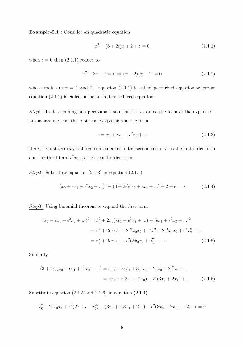
Example-2.1 : Consider an quadratic equation
x2 − (3 + 2ε)x+ 2 + ε = 0 (2.1.1)
when ε = 0 then (2.1.1) reduce to
x2 − 3x+ 2 = 0⇒ (x− 2)(x− 1) = 0 (2.1.2)
whose roots are x = 1 and 2. Equation (2.1.1) is called perturbed equation where as
equation (2.1.2) is called un-perturbed or reduced equation.
Step1 : In determining an approximate solution is to assume the form of the expansion.
Let us assume that the roots have expansion in the form
x = x0 + εx1 + ε2x2 + ... (2.1.3)
Here the first term x0 is the zeroth-order term, the second term εx1 is the first order term
and the third term ε2x2 as the second order term.
Step2 : Substitute equation (2.1.3) in equation (2.1.1)
(x0 + εx1 + ε2x2 + ...)2 − (3 + 2ε)(x0 + εx1 + ...) + 2 + ε = 0 (2.1.4)
Step3 : Using binomial theorem to expand the first term
(x0 + εx1 + ε2x2 + ...)2 = x20 + 2x0(εx1 + ε2x2 + ...) + (εx1 + ε2x2 + ...)2
= x20 + 2εx0x1 + 2ε2x0x2 + ε2x21 + 2ε3x1x2 + ε4x22 + ...
= x20 + 2εx0x1 + ε2(2x0x2 + x21) + ... (2.1.5)
Similarly,
(3 + 2ε)(x0 + εx1 + ε2x2 + ...) = 3x0 + 3εx1 + 3ε2x1 + 2εx0 + 2ε2x1 + ...
= 3x0 + ε(3x1 + 2x0) + ε2(3x2 + 2x1) + ... (2.1.6)
Substitute equation (2.1.5)and(2.1.6) in equation (2.1.4)
x20 + 2εx0x1 + ε2(2x0x2 + x21)− (3x0 + ε(3x1 + 2x0) + ε2(3x2 + 2x1)) + 2 + ε = 0
8
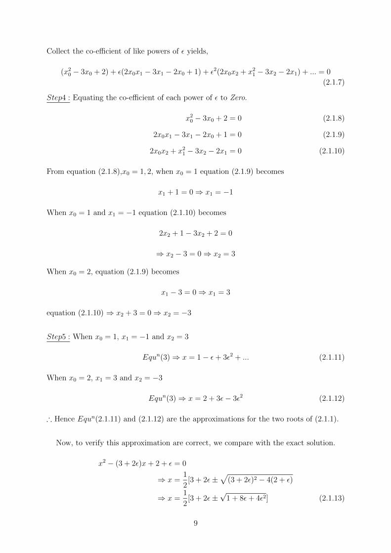
Collect the co-efficient of like powers of ε yields,
(x20 − 3x0 + 2) + ε(2x0x1 − 3x1 − 2x0 + 1) + ε2(2x0x2 + x21 − 3x2 − 2x1) + ... = 0
(2.1.7)
Step4 : Equating the co-efficient of each power of ε to Zero.
x20 − 3x0 + 2 = 0 (2.1.8)
2x0x1 − 3x1 − 2x0 + 1 = 0 (2.1.9)
2x0x2 + x21 − 3x2 − 2x1 = 0 (2.1.10)
From equation (2.1.8),x0 = 1, 2, when x0 = 1 equation (2.1.9) becomes
x1 + 1 = 0⇒ x1 = −1
When x0 = 1 and x1 = −1 equation (2.1.10) becomes
2x2 + 1− 3x2 + 2 = 0
⇒ x2 − 3 = 0⇒ x2 = 3
When x0 = 2, equation (2.1.9) becomes
x1 − 3 = 0⇒ x1 = 3
equation (2.1.10) ⇒ x2 + 3 = 0⇒ x2 = −3
Step5 : When x0 = 1, x1 = −1 and x2 = 3
Equn(3)⇒ x = 1− ε+ 3ε2 + ... (2.1.11)
When x0 = 2, x1 = 3 and x2 = −3
Equn(3)⇒ x = 2 + 3ε− 3ε2 (2.1.12)
∴ Hence Equn(2.1.11) and (2.1.12) are the approximations for the two roots of (2.1.1).
Now, to verify this approximation are correct, we compare with the exact solution.
x2 − (3 + 2ε)x+ 2 + ε = 0
⇒ x =1
2[3 + 2ε±
√(3 + 2ε)2 − 4(2 + ε)
⇒ x =1
2[3 + 2ε±
√1 + 8ε+ 4ε2] (2.1.13)
9

Using binomial theorem, we have
(1 + 8ε+ 4ε2)12 = 1 +
1
2(8ε+ 4ε2) +
(12)(−1
2)
2!(8ε+ 4ε2)2 + ...
= 1 + 4ε+ 2ε2 − 1
8(64ε2 + ...)
= 1 + 4ε+ 2ε2 − 8ε2 + ...
= 1 + 4ε− 6ε2 + ...
Substitute this value in Equn(13), we have
x =1
2(3 + 2ε+ 1 + 4ε− 6ε2 + ...)
= 2 + 3ε− 3ε2 + ...
x =1
2(3 + 2ε− 1− 4ε+ 6ε2 + ...)
= 1− ε+ 3ε2 + ...
Which are same as equation (2.1.11) and (2.1.12).
2.2 Singular Perturbation Theory
It concern the study of problems featuring a parameter for which the solution of the
problem at a limiting value of the parameter are different in character from the limit
of the solution of the general problem. For regular perturbation problems, the solution
of the general problem converge to the solution of the limit problem as the parameter
approaches the limit value.
Example-2.2: Consider,
εx2 + x+ 1 = 0 (2.2.1)
Since equation (2.2.1) is a quadratic equation, it has two roots. For ε −→ 0 Equation
(2.2.1) reduce to
x+ 1 = 0 (2.2.2)
10

Which is of first order. Thus x is discontinuous at ε = 0. Such perturbation are called
singular perturbation problem.
x = x0 + εx1 + ε2x2 + ... (2.2.3)
Putting this value in Equation (1)
ε (x0 + εx1 + ...) + x0 + εx1 + ...+ 1 = 0
⇒ ε(x20 + 2εx0x1 + ...
)+ x0 + εx1 + ...+ 1 = 0
⇒ εx20 + 2ε2x0x1 + ...+ x0 + εx1 + ...+ 1 = 0
⇒ ε(x20 + x1
)+ x0 + 1 = 0
Equating co-efficient of like power of ε gives
x0 + 1 = 0
x1 + x20 = 0
When x0 = −1 , x1 = −1 So one of the root is
x = −1− ε+ ... (2.2.4)
Thus as expected the above procedure yielded only one root. We investigate the exact
solution i.e. ,
x =1
2ε
(−1±
√1− 4ε
)(2.2.5)
Using binomial theorem we have
√1− 4ε = 1− 2ε+
(12)(−1
2)
2!× (−4ε)2 + ...
= 1− 2ε− 2ε2 + ... (2.2.6)
Substituting (6) in (5)
x =−1 + 1− 2ε− 2ε2 + ...
2ε= −1− ε+ ... (2.2.7)
x =−1− 1 + 2ε+ 2ε2 + ...
2ε=−1
ε+ 1 + ε+ ... (2.2.8)
11

Therefore, both of the roots go in powers of ε but one starts with ε−1. Hence it is not
surprising that the assumed expansion in (2.2.3) is failed to produce the root (2.2.8).
consequently one can not determine the second root by a perturbation technique unless
its form is known. In those cases, we recognize that, if the order of the equation is not
to be reduced, the other tends to ∞ as ε −→ 0 and hence, assume that the leading term
has the form
x =y
εv(2.2.9)
Where v must be greater than zero and needs to be determined in the course of analysis.
Substitute (2.2.9) in (2.2.1)
ε1−2vy2 + εvy + 1 + ... = 0
Since v > 0, th second term is much bigger than 1 . Hence the dominant part of (2.2.9) is
ε1−2vy2 + εvy = 0 (2.2.10)
which demands that power of ε be the same.
1− 2v = −v ⇒ v = 1
For v = 1 ⇒ y = o or −1.
The first value y = 0, correspond to the first root x = −1 − ε. For y = −1, it
corresponds to second root. Thus it follows from (2.2.9)
x =−1
ε+ ...
To determine more terms in the expansion of second root, we try
x =−1
ε+ x0 + ... (2.2.11)
Substitute it in equation (2.2.1)
⇒ ε
(−1
ε+ x0 + ...
)2
− −1
ε+ x0 + ...+ 1 = 0
⇒ ε
(−1
ε
2
+2x0ε
+ x20 + ...
)− −1
ε+ x0 + 1 + ... = 0
⇒ −2x0 + x0 + 1 +©(ε) = 0
12

⇒ x0 = 1and equation (2.2.11) becomes
x = −1
ε+ 1 + ...
Alternatively, once v has been determined. We view (2.2.9) as a transformation from x
to y. Then putting x = yε
in (2.2.1) yields,
y2 + y + ε = 0 (2.2.12)
Which can be solved to determine both the roots because ε does not multiply the highest
order.
2.3 Perturbation Theory For Differential Equation
Example-2.3 : Consider,
d2y
dτ 2= −εdy
dτ− 1, y(0) = o,
dy
dτ(0) = 1 (2.3.1)
Let us assume the expansion
y(τ) = y0(τ) + εy1(τ) + ε2y2(τ) +©(ε3) (2.3.2)
Substitute Equation (2.3.2) in (2.3.1)
d2y
dτ 2+ ε
dy
dτ+ 1 = 0
d2
dτ 2(y0(τ) + εy1(τ) + ε2y2(τ) +©(ε3)
)+ ε
d
dτ
(y0(τ) + εy1(τ) + ε2y2(τ) +©(ε3)
)+ 1 = 0
⇒ d2y0dτ 2
+ 1 + ε
(d2y1dτ 2
+dy0dτ
)+ ε2
(d2y2dτ 2
+dy1dτ
)+©(ε3) = 0
Equating the co-efficient of ε , it becomes
⇒ d2y0dτ 2
+ 1 = 0, y0(0) = 0,dy0dτ
(0) = 1
⇒ d2y1dτ 2
+dy0dτ
= 0, y1(0) = 0,dy1dτ
(0) = 0
⇒ d2y2dτ 2
+dy1dτ
= 0, y1(0) = 0,dy1dτ
(0) = 0 (2.3.3)
13
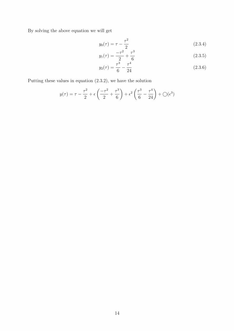
By solving the above equation we will get
y0(τ) = τ − τ 2
2(2.3.4)
y1(τ) =−τ 2
2+τ 3
6(2.3.5)
y2(τ) =τ 3
6− τ 4
24(2.3.6)
Putting these values in equation (2.3.2), we have the solution
y(τ) = τ − τ 2
2+ ε
(−τ 2
2+τ 3
6
)+ ε2
(τ 3
6− τ 4
24
)+©(ε3)
14

CHAPTER 3
3 Homotopy Perturbation Method
In recent years, the Homotopy Perturbation Method has been successfully applied to solve
many types of differential equation. It was proposed by ”Ji-Huan He” in 1999 . Dr. He
used HPM to solve
1. Lighthill equation
2. Duffing equation
3. Non-linear wave equation
4. Schrodinger equation
In the homotopy perturbation technique we will first propose a new perturbation tech-
nique coupled with the homotopy technique. In topology two continuous function from
one topological space to another is called ”homo-topic”. Formally a homotopy between
two continuous function f and g from a topological space X to a topological space Y is
defined to be a continuous function
H : X × [0, 1] −→ Y
such that
H(x, 0) = f(x) and H(x, 1) = g(x) ,∀x ∈ X
The homotopy perturbation method does not depend upon a small parameter in the
equation. By the homotopy technique in topology, a homotopy is constructed with an
embedding parameter p ∈ [0, 1] which is considered as a small parameter.
3.1 Basic idea of HPM
Let us consider the non-linear differential equation
A(u)− f(r) = 0, r ∈ Ω (3.1.1)
15
with boundary condition
B(u,∂u
∂n) , r ∈ Γ (3.1.2)
Where A is a general differential operator , B is a boundary operator. Γ is the boundary
of domain Ω. f(r) is a known analytic function. Now, the operator A can be divided
into two parts L and N , where L is linear and N is non-linear. Equation (3.1.1) can be
written as follows
L(u) +N(u)− F (r) = 0 (3.1.3)
By the homotopy technique, we construct a homotopy
v(r, p) : Ω× [0, 1] −→ R,
Which satisfies
H(v, p) = (1− p)[L(v)− L(u0)] + p[A(v)− f(r)] = 0, p ∈ [0, 1], r ∈ Ω (3.1.4)
or
H(v, p) = L(v)− L(u0 + pL(u0 + p[N(v)− f(r)] = 0
Where, u0 is an initial approximation of equation (3.1.1), which satisfies the boundary
condition. From equation (3.1.4)
H(v, o) = L(v)− L(u0) = 0 (3.1.5)
H(v, 1) = A(v)− f(r) = 0 (3.1.6)
The changing process of p from zero to unity is just that of v(r, p) from u0(r) to u(r). In
topology, this is called deformation and L(v)−L(u0) and A(v)−f(r) are called homotopic.
In this paper, we will first use the embedding parameter p as a small parameter and
assume that the solution of equn(3.1.4) can be written as a power series of p.
v = v0 + pv1 + p2v2 + ... (3.1.7)
setting p = 1, results the approximate solution of equn(3.1.1)
u = limp→1
v = v0 + v1 + v2 + ... (3.1.8)
16

The series (3.1.8) is convergent for most cases, however the convergent rate depends upon
the non-linear operator A(v).
Example 3.2: We will consider the Lighthill equation
(x+ εy)dy
dx+ y = 0, y(1) = 1 (3.2.1)
By the method, we can construct a homotopy which satisfies
(1− p)[εY
dY
dx− εy0
dy0dx
]+ p
[(x+ εy)
dY
dx+ Y
]= 0, p ∈ [0, 1] (3.2.2)
We can obtain a solution of (3.2.2) in the form
Y (x) = Y0(x) + pY1(x) + p2Y2(x) + ... (3.2.3)
Where Yi(x); i = 0, 1, 2, ... are functions yet to be determined. By considering only first
two terms of the above equation substitute equation (3.2.3) into equation (3.2.2)
(1− p)[ε(Y0 + pY1)
(dY0dx
+dY1dx
)− εy0
dy0dx
]+ p
[(x+ εY0 + εpY1)
(dY0dx
+ pdY1dx
)+ (Y0 + pY1)
]= 0
⇒ (1− p)[εY0
(dY0dx
+dY1dx
)+ εpY1
(dY0dx
+dY1dx
)− εy0
dy0dx
]+ p
[(x+ εY0 + εpY1)
(dY0dx
+ pdY1dx
)+ (Y0 + pY1)
]= 0
⇒ εpY1dY1dx
+ (1− p)[εY0
dY0dx− εy0
dy0dx
]+ p
[(x+ εY0)
dY0dx
+ Y0
]+ εp2Y1
(dY0dx
+ pdY1dx
)+ p2Y1 = 0
Now, we get
εY0dY0dx− εy0
dy0dx
= 0 (3.2.4)
εY1dY1dx
+
[(x+ εY0)
dY0dx
+ Y0
]= 0 (5)
The initial approximation Y0(x) or y0(x) can be freely chosen. Here I set
Y0(x) = y0(x) = −xε, Y0(1) = −1
ε(3.2.6)
17

So that, the residual of equation (3.2.1) at x = 0 vanishes. Then substitute equation
(3.2.6) into equation (3.2.5),
εY1dY1dx
+
[(x− εx
ε)dY0dx− x
ε
]= 0
⇒ εY1dY1dx− x
ε= 0
⇒ εY1dY1dx
=x
ε
⇒ ε2Y1dY1 = xdx
Integrating both sides, we get
⇒ ε2Y 21
2=x2
2+ c
⇒ ε2Y 21 = x2 + 2c
⇒ Y1 =
√x2 + 2c
ε
⇒ εY1 =√x2 + 2c (7)
Putting the initial condition Y1(1) = 1− Y0 = 1 + 1ε
,
⇒ ε
(1 +
1
ε
)=√
1 + 2c
⇒ 1 + ε =√
1 + 2c
⇒ 1 + ε2 + 2ε = 1 + 2c
⇒ c =ε2 + 2ε
2
Now, putting this value in equation (3.2.7) we get
Y1 =1
ε
√x2 + 2ε+ ε2
Substitute this value in equn(3.2.3) ,
⇒ Y (x) = Y0(x) + Y1(x) =1
ε
(−x+
√x2 + 2ε+ ε2
)(8)
Which is the exact solution of equn(3.2.1).
18

CHAPTER 4
4 Application Of Homotopy Perturbation Method
4.1 Derivation of Blasius Equation
For a two-dimensional flow, steady state, incompressible flow with zero pressure gradient
over a flat plate, governing equation are simplified to
∂u
∂x+∂v
∂y= 0 (4.1.1)
u∂u
∂x+ v
∂u
∂y= ν
∂2u
∂y2(4.1.2)
subjected to boundary conditions
y = o , u = 0
y =∞ , u = U∞ ,∂u
∂y= 0 (4.1.3)
Take
x∗ =x
L, y∗ =
y
δ, u∗ =
u
U∞, v∗ =
Lv
δU∞, p∗ =
p
ρU2∞
take the stream function ψ defined by
ψ =√νxU∞f(η) (4.1.4)
f is a dimensionless function of the similarity variable η .
η =y√
νx/U∞(4.1.5)
Now,
u =∂ψ
∂y=∂ψ
∂η.∂η
∂y
=√νxU∞f
′(η)1√
νx/U∞
= U∞df
dη(4.1.6)
19
similarly,
v = −∂ψ∂x
= −[∂
∂x
√νxU∞f(η) +
√νxU∞
∂
∂xf(η)
]= −
[f(η)
1
2
√νU∞x
+√νxU∞
df
dη(−1
2)yx−
32√
ν/U∞
]
= −
[1
2f(η)
√νU∞x− 1
2
U∞y
x
df(η)
dη
]
=1
2
√νU∞x
[ηdf
dη− f
](4.1.7)
Now,
∂u
∂x= U∞
d2f
dη2y√ν/U∞
(1
2)x−
32
= −U∞2x
ηd2f
dη2(4.1.8)
∂u
∂y= U∞
d2f
dη2.
1√νx/U∞
=U∞√νx/U∞
.d2f
dη2(4.1.9)
∂2u
∂y2=
∂
∂y
(U∞√νx/U∞
.d2f
dη2
)
=U∞√νx/U∞
(d3f
dη3.
1√νx/U∞
)
=U∞2
νx
d3f
dη3(4.1.10)
Putting this value in equation (4.1.2), we get
u∂u
∂x+ v
∂u
∂y= ν
∂2u
∂y2
⇒ U∞df
dη
[−U∞
2xη
d2f
dη2
]+
1
2
√νU∞x
[ηdf
dη− f
].
U∞√νx/U∞
.d2f
dη2= ν
U∞2
νx
d3f
dη3
⇒ −U2∞
2xηdf
dη.d2f
dη2+
1
2
U2∞x
[ηdf
dη− f
]d2f
dη2=U2∞x.d3f
dη3
⇒ −η2.df
dη.d2f
dη2+η
2.df
dη.d2f
dη2− 1
2f.d2f
dη2=d3f
dη3
20

⇒ d3f
dη3+
1
2f.d2f
dη2= 0 (4.1.11)
With boundary condition,
η = 0 , f =df
dη= 0
η −→∞ ,df
dη= 1 (4.1.12)
4.2 Solution of Blasius Equation By Homotopy Perturbation
Method
So, to get a solution of equation (4.1.11) by the homotopy technique, we construct a
homotopy
v(r, p) : Ω× [0, 1] −→ R,
Which satisfies,
H(v, p) = (1− p)[L(v)− L(u0)] + p[A(v)− f(r)] = 0, p ∈ [0, 1], r ∈ Ω
or
H(v, p) = L(v)− L(u0) + pL(u0) + p[N(v)− f(r)] = 0 (4.2.1)
Where, u0 is an initial approximation of equation (4.2.1), which satisfies the boundary
condition.
Now, from equation (4.1.11)
(1− p)(∂3F
∂η3− ∂3f0
∂η3
)+ p
(∂3F
∂η3+F
2+∂2F
∂η2
)= 0
or, (∂3F
∂η3− ∂3f0
∂η3
)+ p
(∂3f0∂η3
+F
2+∂2F
∂η2
)= 0 (4.2.2)
Suppose that the solution of the equation (4.2.2) to be in the following form
F = F0 + pF1 + p2F2 + ... (4.2.3)
21

Substituting equn(4.2.3) in (4.2.2) we get,
∂3F0
∂η3+ p
∂3F1
∂η3+ p2
∂3F2
∂η3− ∂3f0
∂η3+ p
∂3f0∂η3
+ p
[F0
2
(∂2F0
∂η2+ p
∂2F1
∂η2
)+ p
F1
2
(∂2F0
∂η2+ p
∂2F1
∂η2
)+ ...
]= 0
Re-arranging the co-efficient of the terms with identical powers of p, we have
p0 :∂3F0
∂η3− ∂3f0
∂η3= 0
p1 :∂3F1
∂η3+∂3f0∂η3
+F0
2
∂2F0
∂η2= 0
p2 :∂3F2
∂η3+F1
2
∂2F0
∂η2+F0
2
∂2F1
∂η2= 0
p3 :∂3F3
∂η3+F1
2
∂2F1
∂η2+F2
2
∂2F0
∂η2+F0
2
∂2F2
∂η2= 0 (4.2.4)
. : .
. : .
. : .
First we take F0 = f0. We start iteration by defining f0 as a Taylor series of order two
near η = 0, so that it could be accurate near η = 0.
F0 = f0 =f ′′(0)
2η2 + f ′(0)η + f(0)
Let us take f ′′(0) = 0.332057, [5] and from the given boundary condition f = 0 and
f ′ = 0. So,
f0 =0.332057
2η2
= 0.1660285η2
Now, taking this value to solve F1 from (4.2.4)
∂3F1
∂η3+∂3f0∂η3
+F0
2
∂2F0
∂η2= 0
∂3F1
∂η3= −F0
2
∂2F0
∂η2
= −0.1660285
2η2
∂2
∂η2(0.1660285)η2
∂3F1
∂η3= −(0.1660285)2.η2
F1 = −(0.1660285)2.η5
3.4.5
⇒ F1 = f1 = −0.00045942η5
22

Similarly from (4.2.4) we can easily calculate the value of f2, f3,... as
f2 = 0.00000249η8
f3 = −0.00000001η11 (4.2.5)
For the assumption p=1, we get
f(η) = 0.1660285η2 − 0.00045942η5 + 0.00000249η8 − 0.00000001η11 (4.2.6)
Results:
f(η)
η H.P.M Blasius
0 0 0
0.5 0.0415 0.0415
1 0.16550 0.1656
1.5 0.3701 0.3701
2 0.6500 0.6500
2.5 0.9962 0.9963
3 1.3964 1.3968
3.5 1.8350 1.8377
4.0 2.2897 2.3057
Figure 1: The comparison of answers obtained by H.P.M and Blasius’s results for f(η).
23

f ′(η)
η H.P.M Blasius
0 0 0
0.5 0.1658 0.1659
1 0.3298 0.3298
1.5 0.4867 0.4868
2 0.6297 0.6298
2.5 0.7511 0.7513
3 0.8445 0.8430
3.5 0.9027 0.9130
4.0 0.9028 0.9555
Figure 2: The comparison of answers obtained by H.P.M and Blasius’s results for f ′(η).
24

5 Conclusion
In this research project paper, we have studied a well known Blasius boundary layer
equation. We have applied homotopy perturbation method to solve this non-linear differ-
ential equation. From fig. 1 we conclude that the obtained results for f(η) have excellent
accuracy with the Blasius solution of Howarth [2]. Similarly in fig. 2 we also have approx-
imate accuracy for f ′(η). The proposed method does not require small parameters in the
equations, so the limitation of the traditional perturbation technique can be eliminated.
The initial approximation can be freely selected with possible unknown constants. The
approximation obtained by this method are valid not only for small parameter, but also
for every large parameters. So, the homotopy perturbation method can applied to various
non-liner differential equation. In this project paper, I came to know about perturbation
method and homotopy perturbation method to solve various non-linear differential equa-
tion. I also learned the latex software to write mathematical code. In my future work I
will employed all this methods so that I can solve any non-linear problems easily.
25

References
[1] Nayfeh, A.H., Introduction to perturbation technique, Wiley, New York, 1981.
[2] Howarth, L., On the solution of the Laminar Boundary-Layer Equations, Proceedings
of the Royal Society of London, A.164:1983, 547-549 .
[3] He, J.H., Homotopy perturbation technique, Computer Methods in Applied Mechanics
and Engineering. Vol.178, 1999, 257-262 .
[4] He, J.H., Homotopy perturbation method for solving boundary value problems.
Physics letters A Vol.350, 2006, 87-88, .
[5] Ganji, D.D., Soleimani, S., Gorji, M., New application of homotopy perturbation
method, International journal of nonlinear science and numerical simulation Vol.8(3):
2007, (319) .
[6] Ganji, D.D., Babazadeh, H., Noori F., Pirouz, M.M., Janipour M., An application of
homotopy perturbation method for non-linear Blasius equation to boundary layer flow
over a flat plate, International Journal of Non-linear Science, Vol.7, 2009, 399-404 .
[7] Babolian E., Saeidian J., Azizi A., Application of homotopy perturbation method to
solve non-linear problems, Applied Mathematical sciences, Vol.3, 2009, 2215-2226 .
[8] Taghipour R., Application of homotopy perturbation method on some linear and non-
linear periodic equations, World Applied Sciences Journal, Vol.10, 2010, 1232-1235
.
26


