

Sparsity-promoting optimal control of
power networks
A DISSERTATION
SUBMITTED TO THE FACULTY OF THE GRADUATE SCHOOL
OF THE UNIVERSITY OF MINNESOTA
BY
Xiaofan Wu
IN PARTIAL FULFILLMENT OF THE REQUIREMENTS
FOR THE DEGREE OF
Doctor of Philosophy
December 2016

Sparsity-promoting optimal control of
power networks
Copyright © 2016
by
Xiaofan Wu
ALL RIGHTS RESERVED

To Jingyi and my parents
i

Acknowledgements
I would like to express my sincere gratitude to my advisor Professor Mihailo R. Jovanovic
for his utmost support and guidance throughout the years of my graduate study. It is
my greatest pleasure to have Mihailo as my academic teacher, research mentor, spiritual
guide, soccer teammate and gym buddy. Those tremendous time that we spent together
on brain storming, paper writing, problem solving, gym exercising, will be my most
precious memories forever. His patience, motivation, enthusiasm, immense knowledge
and commitment to excellence has always inspired me to be a better student and a
better person.
I am extremely fortunate to have the opportunity to work with Professor Florian
Dorfler for the past three years. His creativity and patience have made our collaboration
possible. His insightful comments and suggestions have made our joint work successful.
I am truly thankful to him for inviting me to Automatic Control Lab at ETH Zurich as
a visiting scholar.
I owe sincere thankfulness to Professor Sairaj Dhople, Peter Seiler, Jarvis Haupt
for serving on my defense committee. I have benefited from interacting with them and
learned the knowledge that I need for completing my graduate study.
I am very grateful to have my labmates and friends: Dr. Fu Lin, Dr. Rashad
Moarref, Dr. Binh Lieu, Dr. Armin Zare, Dr. Neil Dhingra, Dr. Yongxin Chen, Sepideh
Hassan-Moghaddam, Wei Ran, Dongsheng Ding, Hamza Farooq, Karen Khatamifard,
Dr. Sei Zhen Khong, Dr. Kaoru Yamamoto, Dr. Rohit Gupta, Dr. Marcello Colombino,
and many other friends who have helped me. They have made my graduate study at
UMN meaningful and colorful. I would like to thank Fu Lin for his generous help and
guidance during my first years in Minnesota. I am very grateful to Binh Lieu for hosting
all the warm and fun holiday events. I would like to express my special thanks to my
ii

best buddies, Armin and Neil, for all the fun we had during these graduate school years.
It has been the greatest privilege to have my Chinese friends and buddies: Wei
Zhang, Keping Song, Yinglong Feng, Yi Wang, Zisheng Zhang, Jie Kang, Yu Chen, Jun
Fang, Cong Ma, Kejian Wu, Huanan Zhang, Peng Peng and many others. They have
become an important part of my life in Minnesota. I will always remember the great
times we have spent together.
I would like to sincerely thank my family. My parents have always been teaching
me to study hard, work hard, party hard and enjoy life. They always encourage me and
cheer me up when I am down. They always guide me through difficult time and help
me pursue my dreams. Without their unconditional support, I would not be the person
I am today.
Finally, I would like to extend my warmest thanks to the love of my life, my wife
Jingyi Zhang. She has been my soul mate and my best friend. Throughout the years,
she has been on my side, supporting me, helping me, trusting me and loving me. Her
company and encouragement has made this dissertation possible.
iii

Abstract
In this dissertation, we study the problems of structure design and optimal control
of consensus and synchronization networks. Our objective is to design controller that
utilize limited information exchange between subsystems in large-scale networks. To ob-
tain controllers with low communication requirements, we seek solutions to regularized
versions of the H2 optimal control problem. The proposed framework can be leveraged
for control design in applications like wide-area control in bulk power systems, frequency
regulation in power system/microgrids, synchronization of nonlinear oscillator networks,
etc. The structure of the dissertation is organized as follows.
In Part I, we focus on the optimal control problems in systems with symmetries and
consensus/synchronization networks. They are characterized by structural constraints
that arise either from the underlying group structure or the lack of the absolute mea-
surements for a part of the state vector. Our framework solves the regularized versions
of the H2 optimal control problems that allow the state-space representations that are
used to quantify the system’s performance and sparsity of the controller to be expressed
in different sets of coordinates. For systems with symmetric dynamic matrices, the
problem of minimizing the H2 or H∞ performance of the closed-loop system can be
cast as a convex optimization problem. Studying the symmetric component of a gen-
eral system’s dynamic matrices provides bounds on the H2 and H∞ performance of the
original system.
Part II studies wide-area control of inter-area oscillations in power systems. Our
input-output analysis examines power spectral density and variance amplification of
stochastically forced systems and offers new insights relative to modal approaches. To
improve upon the limitations of conventional wide-area control strategies, we also study
the problem of signal selection and optimal design of sparse and block-sparse wide-
area controllers. We show how different sparsity-promoting penalty functions can be
used to achieve a desired balance between closed-loop performance and communica-
tion complexity. In particular, we demonstrate that the addition of certain long-range
communication links and careful retuning of the local controllers represent an effective
iv

means for improving system performance.
In Part III, we apply the sparsity-promoting optimal control framework to two prob-
lem encounters in distributed networks. First, we consider the optimal frequency reg-
ulation problem in power systems and propose a principled heuristic to identify the
structure and gains of the distributed integral control layer. We define the proposed dis-
tributed PI-controller and formulate the resulting static output-feedback control prob-
lem. Second, we develop a structured optimal-control framework to design coupling
gains for synchronization of weakly nonlinear oscillator circuits connected in resistive
networks with arbitrary topologies. The structured optimal-control problem allows us
to seek a decentralized control strategy that precludes communications between the
weakly nonlinear Lienard-type oscillators.
v

Contents
Acknowledgements ii
Abstract iv
List of Tables x
List of Figures xi
1 Introduction 1
1.1 Motivation . . . . . . . . . . . . . . . . . . . . . . . . . . . . . . . . . . 1
1.2 Main topics of the dissertation . . . . . . . . . . . . . . . . . . . . . . . 3
1.2.1 Optimal sparse feedback design . . . . . . . . . . . . . . . . . . . 3
1.2.2 Sparsity-promoting optimal control of systems with invariances
and symmetries . . . . . . . . . . . . . . . . . . . . . . . . . . . . 4
1.2.3 Wide-area control in power systems . . . . . . . . . . . . . . . . 5
1.2.4 Distributed-PI control in power systems . . . . . . . . . . . . . . 8
1.2.5 Design of optimal coupling gains for synchronization of nonlinear
oscillators . . . . . . . . . . . . . . . . . . . . . . . . . . . . . . . 10
1.3 Dissertation structure . . . . . . . . . . . . . . . . . . . . . . . . . . . . 11
1.4 Contributions of the dissertation . . . . . . . . . . . . . . . . . . . . . . 13
I Sparsity-promoting optimal control 16
2 Optimal Sparse Feedback Design 17
2.1 Motivation and background . . . . . . . . . . . . . . . . . . . . . . . . . 17
vi

2.1.1 Problem formulation . . . . . . . . . . . . . . . . . . . . . . . . . 19
2.1.2 Examples . . . . . . . . . . . . . . . . . . . . . . . . . . . . . . . 20
2.1.3 Sparsity-promoting penalty functions . . . . . . . . . . . . . . . . 23
2.2 Class of convex problems . . . . . . . . . . . . . . . . . . . . . . . . . . 24
2.3 Design of controller structure . . . . . . . . . . . . . . . . . . . . . . . . 26
2.3.1 Structure design via ADMM . . . . . . . . . . . . . . . . . . . . 26
2.3.2 Polishing step . . . . . . . . . . . . . . . . . . . . . . . . . . . . . 31
2.4 Case study: synchronization network . . . . . . . . . . . . . . . . . . . . 31
2.5 Concluding remarks . . . . . . . . . . . . . . . . . . . . . . . . . . . . . 34
3 Sparsity-promoting optimal control of systems with invariances and
symmetries 36
3.1 Problem formulation . . . . . . . . . . . . . . . . . . . . . . . . . . . . . 37
3.1.1 Applications . . . . . . . . . . . . . . . . . . . . . . . . . . . . . 38
3.2 Symmetric system design . . . . . . . . . . . . . . . . . . . . . . . . . . 39
3.2.1 Convex optimal control for symmetric systems . . . . . . . . . . 40
3.2.2 Stability and performance guarantees . . . . . . . . . . . . . . . 41
3.2.3 Approximation bounds . . . . . . . . . . . . . . . . . . . . . . . . 43
3.3 Computational advantages for structured problems . . . . . . . . . . . . 43
3.3.1 Spatially-invariant systems . . . . . . . . . . . . . . . . . . . . . 45
3.4 Examples . . . . . . . . . . . . . . . . . . . . . . . . . . . . . . . . . . . 46
3.4.1 Directed Consensus Network . . . . . . . . . . . . . . . . . . . . 46
3.4.2 Swift-Hohenberg Equation . . . . . . . . . . . . . . . . . . . . . . 46
3.5 Concluding remarks . . . . . . . . . . . . . . . . . . . . . . . . . . . . . 50
II Wide-area control of power systems 51
4 Decentralized optimal control of inter-area oscillations 52
4.1 Modeling and control preliminaries . . . . . . . . . . . . . . . . . . . . . 52
4.1.1 Swing equations . . . . . . . . . . . . . . . . . . . . . . . . . . . 53
4.1.2 Problem formulation . . . . . . . . . . . . . . . . . . . . . . . . . 53
4.2 Input-output analysis . . . . . . . . . . . . . . . . . . . . . . . . . . . . 56
vii

4.2.1 Power spectral density and variance amplification . . . . . . . . . 56
4.3 Sparse and block-sparse optimal control . . . . . . . . . . . . . . . . . . 58
4.3.1 Elementwise sparsity . . . . . . . . . . . . . . . . . . . . . . . . . 58
4.3.2 Block sparsity . . . . . . . . . . . . . . . . . . . . . . . . . . . . . 59
4.4 Case study: IEEE 39 New England model . . . . . . . . . . . . . . . . . 62
4.4.1 Analysis of the open-loop system . . . . . . . . . . . . . . . . . . 63
4.4.2 Sparsity-promoting optimal wide-area control . . . . . . . . . . . 65
4.4.3 Comparison of open- and closed-loop systems . . . . . . . . . . . 69
4.4.4 Robustness analysis . . . . . . . . . . . . . . . . . . . . . . . . . 72
4.5 Concluding remarks . . . . . . . . . . . . . . . . . . . . . . . . . . . . . 74
III Optimal control in distributed networks 76
5 Design of distributed integral control action in power networks 77
5.1 Synchronous frequency and power sharing . . . . . . . . . . . . . . . . . 78
5.2 Distributed integral control . . . . . . . . . . . . . . . . . . . . . . . . . 79
5.2.1 Problem setup . . . . . . . . . . . . . . . . . . . . . . . . . . . . 79
5.2.2 Static output-feedback control problem . . . . . . . . . . . . . . 81
5.2.3 Optimal design of the centralized integral action . . . . . . . . . 85
5.3 Sparsity-promoting optimal control . . . . . . . . . . . . . . . . . . . . . 86
5.4 Case study: IEEE 39 New England model . . . . . . . . . . . . . . . . . 89
5.5 Concluding remarks . . . . . . . . . . . . . . . . . . . . . . . . . . . . . 91
6 Design of optimal coupling gains for synchronization of nonlinear os-
cillators 92
6.1 System of coupled weakly nonlinear oscillator circuits . . . . . . . . . . 93
6.1.1 Nonlinear oscillator model . . . . . . . . . . . . . . . . . . . . . . 93
6.1.2 Resistive electrical network . . . . . . . . . . . . . . . . . . . . . 95
6.1.3 System dynamical model in polar coordinates . . . . . . . . . . . 97
6.1.4 State-space representation of linearized system . . . . . . . . . . 97
6.2 Design of current gains . . . . . . . . . . . . . . . . . . . . . . . . . . . . 100
6.2.1 Linear quadratic control design . . . . . . . . . . . . . . . . . . . 100
viii

6.2.2 Sparsity-promoting optimal control . . . . . . . . . . . . . . . . . 101
6.3 Case study . . . . . . . . . . . . . . . . . . . . . . . . . . . . . . . . . . 102
6.3.1 Optimal current-gain design . . . . . . . . . . . . . . . . . . . . . 104
6.3.2 Time-domain simulations for original nonlinear and linearized mod-
els . . . . . . . . . . . . . . . . . . . . . . . . . . . . . . . . . . . 105
6.4 Concluding remarks . . . . . . . . . . . . . . . . . . . . . . . . . . . . . 105
References 106
ix

List of Tables
4.1 Poorly-damped modes of New England model . . . . . . . . . . . . . . . 63
x

List of Figures
1.1 (a) Fishes utilize local relative distance measurements to form a fish
school. (b) Computers achieve clock synchronization by exchanging local
information in cyber networks. (c) Satellites measure relative distances
between each other to maintain formations. (d) Generators exchange
relative angle/frequency information to achieve synchronization. . . . . 2
1.2 A few typical inter-area oscillations in Europe. . . . . . . . . . . . . . . 6
1.3 (a) Fully-decentralized control strategies implemented locally, ineffective
against inter-area oscillations. (b) Distributed wide-area control using
remote signals, effective against inter-area oscillations. . . . . . . . . . 7
2.1 Topology of a disconnected plant network with 3 clusters and 20 nodes. 32
2.2 Topology of controller network for different values of γ. Edges in the
controller network are marked with red lines. . . . . . . . . . . . . . . . 33
2.3 Sparsity pattern of K for γ = 1. . . . . . . . . . . . . . . . . . . . . . . . 33
2.4 Performance vs sparsity comparison with respect to the optimal central-
ized controller Kc for 50 logarithmically-spaced points γ ∈ [ 10−3 , 1 ]. . . 34
2.5 Performance degradation comparison of K resulting from our framework
(dots) to the average of 100 feedback matrices of random sparsity patterns
with same sparsity level for each γ. . . . . . . . . . . . . . . . . . . . . . 34
3.1 Directed network (black solid arrows) with added undirected edges (
red dashed arrows). Both the H2 and H∞ optimal structured control
problems yielded the same set of added edges. In addition to these edges,
the controllers tuned the weights of the edges (1)− (3) and (1)− (5). . . 47
3.2 H2 and H∞ performance of the closed-loop symmetric system and the
original system subject to a controller designed at various values of γ. . 48
xi

3.3 Computation time for the general formulation (3.4) (blue ◦) and that
which takes advantage of spatial invariance (3.6) ( red ∗). . . . . . . . . 49
3.4 Feedback gain v(x) for the node at position x = 0, computed with N = 51
and γ = 0 (black solid), γ = 0.1 (blue dashed), and γ = 10 ( red dotted). 49
4.1 Block structure of the feedback matrix K. • denote relative angle feed-
back gains, • and • represent local and inter-generator frequency and
PSS gains, respectively. . . . . . . . . . . . . . . . . . . . . . . . . . . . 60
4.2 Structural identity matrix Is with • representing locations of 1’s. . . . . 62
4.3 The IEEE 39 New England Power Grid and its coherent groups identified
using slow coherency theory. . . . . . . . . . . . . . . . . . . . . . . . . . 62
4.4 Polar plots of the angle components of the six poorly-damped modes for
the open-loop system. . . . . . . . . . . . . . . . . . . . . . . . . . . . . 64
4.5 (a) Power spectral density of the open-loop system; (b) zoomed version
of the red square shown in (a). Red dots denote poorly-damped modes
from Table 4.1. . . . . . . . . . . . . . . . . . . . . . . . . . . . . . . . . 64
4.6 Diagonal elements of the open-loop covariance matrix Z1 determine con-
tribution of each generator to the variance amplification. . . . . . . . . . 65
4.7 (a) Eigenvalues; and (b)-(d) eigenvectors corresponding to the three largest
eigenvalues λi of the open-loop output covariance matrix Z1. . . . . . . 66
4.8 Sparsity patterns of K resulting from (SP). . . . . . . . . . . . . . . . . 67
4.9 Performance vs sparsity comparison of sparse K and the optimal central-
ized controller Kc for 50 logarithmically-spaced points γ ∈ [ 10−4 , 0.25 ]. 68
4.10 Sparsity patterns of K resulting from (4.8). . . . . . . . . . . . . . . . . 68
4.11 Performance vs sparsity comparison of block-sparse K and the optimal
centralized controller Kc for 50 logarithmically-spaced points γ = γθ =
γr ∈ [ 10−4 , 0.25 ]. . . . . . . . . . . . . . . . . . . . . . . . . . . . . . . 69
xii

4.12 The eigenvalues of the open-loop system and the closed-loop systems with
sparse/block-sparse/centralized controllers are represented by ∗, ◦, �, and
2, respectively. The damping lines indicate lower bounds for damping
ratios and they are represented by dashed lines using the same colors as
for the respective eigenvalues. The 10% damping line is identified by cyan
color. The numbered black asterisks correspond to the six poorly-damped
modes given in Table 4.1. . . . . . . . . . . . . . . . . . . . . . . . . . . 70
4.13 Power spectral density comparison. . . . . . . . . . . . . . . . . . . . . . 70
4.14 Eigenvalues of the output covariance matrix Z1. ∗ represents the open-
loop system, ◦, � and 2 represent the closed-loop systems with sparse,
block-sparse, and optimal centralized controllers, respectively. . . . . . . 71
4.15 Time-domain simulations of the linearized model of the IEEE 39 New
England power grid. The rotor angles and frequencies of all generators are
shown. The closed-loop results are obtained using the fully-decentralized
block-sparse controller. The initial conditions are given by the eigenvec-
tors of the poorly-damped inter-area modes 2 (left) and 6 (right) from
Table 4.1. . . . . . . . . . . . . . . . . . . . . . . . . . . . . . . . . . . . 72
4.16 Performance histograms of open- and closed-loop linearized systems (with
nominal controllers) for 10, 000 uniformly distributed operating points. . 73
4.17 Multivariable phase margins as a function of γ. . . . . . . . . . . . . . . 74
5.1 The IEEE 39 New England Power Grid. . . . . . . . . . . . . . . . . . . 90
5.2 Sparsity pattern of G resulting from (SP). . . . . . . . . . . . . . . . . . 90
5.3 Performance vs sparsity comparison of sparse G and the optimal central-
ized controller Gc for 50 logarithmically-spaced points γ ∈ [ 10−3 , 10 ]. . 91
6.1 The Van der Pol oscillator circuit with a current gain κ admits the dy-
namics in (6.1). In this case, ω = 1/√LC, ε =
√L/C, and h(v) =
∫f(v)dv = αω(v − βv3/3) where α and β are positive real constants. . . 94
6.2 Kron reduction illustrated for a network of three oscillators. In this
example, A = {1, . . . , 5}, N = {1, 2, 3}, and I = {4, 5}. . . . . . . . . . 97
xiii

6.3 Sparsity-promoting optimal current gain design illustrated for a Kron-
reduced network and two oscillators. As the sparsity emphasis γ in-
creases, K becomes sparser and we eventually recover a diagonal matrix,
Kd, which corresponds to local current gains. Dotted lines indicate com-
munication links that correspond to dense feedback gain matrices. . . . 101
6.4 Schematic diagram of the electrical network. The topology is adopted
from the IEEE 37-bus network. . . . . . . . . . . . . . . . . . . . . . . . 102
6.5 Evolution of averaged amplitudes and phases with time for the nonlinear
system in (6.11). . . . . . . . . . . . . . . . . . . . . . . . . . . . . . . . 103
6.6 Performance versus sparsity comparison of sparse K and the optimal
centralized controller Kc. . . . . . . . . . . . . . . . . . . . . . . . . . . 103
6.7 Oscillator terminal-voltage magnitudes with designed current gains ap-
plied at time t = 0.1 s. . . . . . . . . . . . . . . . . . . . . . . . . . . . . 104
xiv

Chapter 1
Introduction
1.1 Motivation
This dissertation studies structure design and optimal control problems arise in dis-
tributed systems and consensus networks. In large networks of dynamical systems cen-
tralized information processing may impose heavy communication and computation
burden on individual subsystems. This motivates the development of localized feedback
control strategies that require limited information exchange between the subsystems in
order to reach consensus or guarantee synchronization. These problems are encoun-
tered in a number of applications ranging from biology to computer science to power
systems [1–11], see Fig. 1.1 for some examples. In each of these applications, it is of
interest to reach an agreement or to achieve synchronization by exchanging relative
information between the subsystems. The restriction on the absence of the absolute
measurements imposes structural constraints for the analysis and design.
Conventional optimal control of distributed systems relies on centralized implemen-
tation of control policies [12]. In large networks of dynamical systems centralized in-
formation processing may impose heavy communication and computation burden on
individual nodes. This motivates the development of localized feedback control strate-
gies that require limited information exchange between the nodes in order to reach
consensus or guarantee synchronization [2, 3, 5, 6, 10,11,13].
In this dissertation, our objective is to design controller structures and resulting
1

2
(a) (b)
(c) (d)
Figure 1.1: (a) Fishes utilize local relative distance measurements to form a fish school.(b) Computers achieve clock synchronization by exchanging local information in cybernetworks. (c) Satellites measure relative distances between each other to maintainformations. (d) Generators exchange relative angle/frequency information to achievesynchronization.
control strategies that utilize limited information exchange between subsystems in large-
scale networks. To design networks with low communication requirements, we seek
solutions to the regularized version of the standard H2 optimal control problem. Such
solutions trade off network performance and sparsity of the controller. For example,
in the context of wide-area control of power systems [14–16], the optimal controller
respects the structure of the original power network: in both open- and closed-loop
systems, only relative rotor angle differences between different generators appear in the

3
state-space representation.
1.2 Main topics of the dissertation
In this section, we discuss the main topics of the dissertation.
1.2.1 Optimal sparse feedback design
In large networks of dynamical systems centralized information processing may impose
prohibitively expensive communication and computation burden [17,18]. This motivates
the development of theory and techniques for designing distributed controller architec-
tures that lead to favorable performance of large-scale networks. Recently, regularized
versions of standard optimal control problems were introduced as a means for achieving
this goal [19–23]. For example, in consensus and synchronization networks, it is of in-
terest to achieve desired objective using relative information exchange between limited
subset of nodes [1–11].
The objective is to design controllers that provide a desired tradeoff between the
network performance and the sparsity of the static output-feedback controller. This is
accomplished by regularizing the H2 optimal control problem with a penalty on commu-
nication requirements in the distributed controller. In contrast to previous work [19–21],
this regularization penalty reflects the fact that sparsity should be enforced in a spe-
cific set of coordinates. In [19–21], the elements of the state-feedback gain matrix were
taken to represent communication links. Herein, we present a unified framework where
a communication link is a linear function of the elements of the output-feedback gain
matrix.
The proposed framework addresses challenges that arise in systems with invariances
and symmetries, as well as consensus and synchronization networks. For example, the
block diagonal structure of spatially-invariant systems in the spatial frequency domain
facilitates efficient computation of the optimal centralized controllers [17]. However,
since the sparsity requirements are typically expressed in the physical space, it is chal-
lenging to translate them into frequency domain specifications. Furthermore, in wide-
area control of power networks [14–16], it is desired to design the controllers that respect

4
the structure of the original system: in both open- and closed-loop networks, only rel-
ative rotor angle differences between different generators are allowed to appear. To
deal with these structural requirements, we introduce a coordinate transformation to
eliminate the average mode and assure stabilizability and detectability of the remaining
modes. Once again, it is desired to promote sparsity of the feedback gain in physical
domain and it is challenging to translate these requirements in the transformed set of
coordinates.
We leverage the alternating direction method of multipliers (ADMM) [24] to ex-
ploit the structure of the corresponding objective functions in the regularized optimal
control problem. ADMM alternates between optimizing the closed-loop performance
and promoting sparsity of the feedback gain matrix. The sparsity promoting step in
ADMM has an explicit solution and the performance optimization step is solved using
Anderson-Moore and proximal gradient methods. Our framework thus allows for per-
formance and sparsity requirements to be expressed in different set of coordinates and
facilitates efficient computation of sparse static output-feedback controllers.
For undirected consensus networks, the proposed approach admits a convex charac-
terization. Furthermore, for systems with invariances and symmetries, transform tech-
niques are utilized to gain additional computational advantage and improve efficiency.
For example, by bringing matrices in a state-space representation of a spatially invari-
ant systems into block-diagonal forms, the regularized optimal control problem amounts
to easily parallelizable task of solving a sequence of smaller, fully-decoupled problems.
While computational complexity of the algorithms that do not exploit spatially-invariant
structure increases cubicly with the number of subsystems, our algorithms exhibit a lin-
ear growth. After having identified a controller structure, the structured design step
optimizes the network performance over the identified structure.
1.2.2 Sparsity-promoting optimal control of systems with invariances
and symmetries
Structured control problems are, in general, challenging and nonconvex. Many recent
works have identified classes of systems for which structured optimal control problems
can be cast in convex forms. These include funnel causal and quadratically invariant sys-
tems [25,26], positive systems [27,28], structured and sparse consensus/synchronization

5
networks [2,11,29–32], optimal sensor/actuator selection [33,34], and symmetric modi-
fications to symmetric linear systems [35].
In many large-scale problems, controller structure is vitally important. As such,
much effort has been devoted to developing scalable algorithms for nonconvex regu-
larized H2 and H∞ design problems [19, 21–23, 33, 34, 36, 37]. Although many recent
works have developed efficient algorithms for the nonconvex regularized H2 problems,
in general, regularized H∞ problems are difficult because the H∞ norm is nonsmooth.
We propose a principled approach to general regularized H2 and H∞ optimal con-
troller design. Our formulation treats control problems that minimize the H2 or H∞norm by modifying the dynamical generator of a linear system, such as in linear state
feedback. In this part, we use symmetries in system structure to form convex problems
and gain computational advantage.
The contributions are twofold. First, in a similar vein as [35], we utilize the sym-
metric component of a general linear system to form a symmetric system for which the
regularized H2 and H∞ optimal control problems are convex. We implement the con-
trollers designed by this method on the original system. We show that this procedure
guarantees stability and that the closed-loop H2 and H∞ performance of the symmetric
system is an upper bound on the closed-loop H2 and H∞ performance of the original
system.
Second, we provide a way to gain computational advantage by exploiting the block-
diagonalizability of large scale systems. Such a structure arises, for example, in spatially-
invariant systems [17]. In [38], the authors took advantage of this property to develop
an efficient and scalable algorithm for sparsity-promoting feedback design. When a
spatially-invariant system is subject to a spatially-invariant control law, the dynamics
of the system can be represented as the sum of independent subsystems, making the
problem amenable to distributed optimization.
1.2.3 Wide-area control in power systems
Inter-area oscillations in bulk power systems are associated with the dynamics of power
transfers and involve groups of synchronous machines that oscillate relative to each
other. Figure 1.2 These system-wide oscillations arise from modular network topologies,
heterogeneous machine dynamics, adversely interacting controllers, and large inter-area

6
power transfers. With increased system loads and deployment of renewables in re-
mote areas, long-distance power transfers will eventually outpace the addition of new
transmission facilities. This induces severe stress and performance limitations on the
transmission network and may even cause instability and outages [39].
0.5Hz
0.7Hz
0.22Hz
0.15Hz
0.33Hz
0.48Hz
0.8Hz
0.26Hz
Figure 1.2: A few typical inter-area oscillations in Europe.
Traditional analysis and control of inter-area oscillations is based on modal ap-
proaches [40,41]. Typically, inter-area oscillations are identified from the spatial profiles
of eigenvectors and participation factors of poorly damped modes [42, 43], and they
are damped via decentralized controllers, whose gains are carefully tuned using root
locus [44, 45], pole placement [46], adaptive [47], robust [48], and optimal [49] control
strategies. To improve upon the limitations of decentralized control, recent research
centers at distributed wide-area control strategies that involve the communication of
remote signals [50, 51]. See Fig. 1.3 for a comparison between conventional decentral-
ized control and wide-area control strategies. The wide-area control signals are typically
chosen to maximize modal observability metrics [52,53], and the control design methods
range from root locus criteria to robust and optimal control approaches [54–56].
The spatial profiles of the inter-area modes together with modal controllability and
observability metrics were previously used to indicate which wide-area links need to be
added and how supplemental damping controllers have to be tuned. Here, we depart
from the conventional modal approach and propose a novel methodology for analysis and
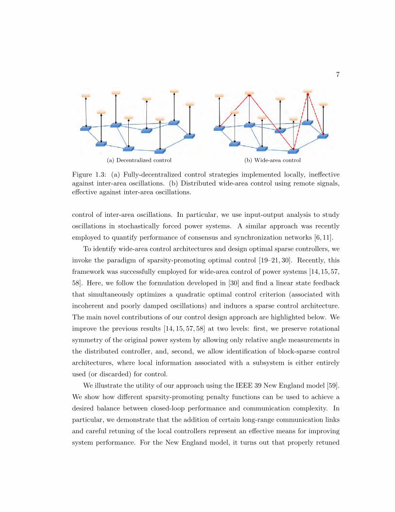
7
(a) Decentralized control (b) Wide-area control
Figure 1.3: (a) Fully-decentralized control strategies implemented locally, ineffectiveagainst inter-area oscillations. (b) Distributed wide-area control using remote signals,effective against inter-area oscillations.
control of inter-area oscillations. In particular, we use input-output analysis to study
oscillations in stochastically forced power systems. A similar approach was recently
employed to quantify performance of consensus and synchronization networks [6, 11].
To identify wide-area control architectures and design optimal sparse controllers, we
invoke the paradigm of sparsity-promoting optimal control [19–21, 30]. Recently, this
framework was successfully employed for wide-area control of power systems [14,15,57,
58]. Here, we follow the formulation developed in [30] and find a linear state feedback
that simultaneously optimizes a quadratic optimal control criterion (associated with
incoherent and poorly damped oscillations) and induces a sparse control architecture.
The main novel contributions of our control design approach are highlighted below. We
improve the previous results [14, 15, 57, 58] at two levels: first, we preserve rotational
symmetry of the original power system by allowing only relative angle measurements in
the distributed controller, and, second, we allow identification of block-sparse control
architectures, where local information associated with a subsystem is either entirely
used (or discarded) for control.
We illustrate the utility of our approach using the IEEE 39 New England model [59].
We show how different sparsity-promoting penalty functions can be used to achieve a
desired balance between closed-loop performance and communication complexity. In
particular, we demonstrate that the addition of certain long-range communication links
and careful retuning of the local controllers represent an effective means for improving
system performance. For the New England model, it turns out that properly retuned
8
and fully-decentralized controllers can perform almost as well as the optimal central-
ized controllers. Our results thus provide a constructive answer to the much-debated
question of whether locally observable oscillations in a power network are also locally
controllable [60].
1.2.4 Distributed-PI control in power systems
The basic task of power system operation is to match load and generation. In an
AC power grid, the synchronous frequency is a direct measure of the load-generation
imbalance, which makes frequency control the fundamental power balancing mechanism.
This task is traditionally accomplished by adjusting generation in a hierarchical three-
layer structure: primary (droop control), secondary (automatic generation control) and
tertiary (economic dispatch) layer, from fast to slow timescales, and from decentralized
to centralized architectures [61, 62]. With the increasing penetration of distributed
generation based on renewables, power systems are subject to larger and faster frequency
fluctuations which have to be compensated by more and more small-scale and distributed
generators. Thus, primary, secondary, and tertiary control tasks have to be handled in
an increasing plug-and-play fashion, that is, using only local measurements, private
model information, and without time-scale separations [63].
From a control-theoretic perspective, the three frequency control layers essentially
correspond to proportional-integral (PI) control and set-point scheduling to solve a re-
source allocation problem. A broad range of research efforts have recently been put
forward to decentralize these control tasks. While the primary layer is typically be-
ing implemented by means of proportional droop control, the secondary and tertiary
integral and set-point controllers can be realized in a plug-and-play fashion through
discrete-time averaging algorithms [64], continuous-time optimization approaches [65],
or distributed averaging-based proportional-integral (DAPI) controllers [66]; see [67] for
a recent literature review. Here, we focus on the simple yet effective DAPI controllers
advocated, among others, in [66–70] to coordinate the action of multiple integral con-
trollers through continuous averaging of the marginal injection costs to arrive at an
optimal solution for a tertiary resource allocation problem.
More generally, PI control is a simple and effective method, it is well known for its
ability to eliminate the influence of static control errors and constant disturbances, and it

9
is commonly used in many industrial applications [71,72]. For large-scale distributed sys-
tems DAPI-type control strategies have been used successfully for stabilization, distur-
bance rejection, and resource allocation, as summarized above for power systems [66–70]
as well as for general network flow problems and other applications [73,74]. DAPI-type
control strategies have also been studied from a pure theoretic perspective as natural
extension to proportional consensus control; see [75,76] and the seminal paper [77].
A common theme of the above studies on various DAPI-type controllers is that
the communication network among the integral controllers needs to be connected to
achieve stable disturbance rejection and resource allocation. However, to the best of
our knowledge, there are no studies addressing the question of how to optimally design
the cyber integral control network relative to the physical dynamics and interactions.
Here, we pursue this question for the special case of frequency regulation in a power
system and using the DAPI controllers advocated in [66,67,69,70,78–80].
In this section, we identify topology of the integral control communication graph and
design the corresponding edge weights for the DAPI controller. In previous studies, the
common assumption on the controller graph being undirected appears overly restric-
tive and requires many communication resources. Our proposed approach allows us to
identify stabilizing and optimal integral controllers with a sparse and directed commu-
nication architecture. As a preliminary pre-processing step, we introduce a coordinate
transformation to enforce the structural constraints on the rotor angles and auxiliary
integral states. In the new set of coordinates, the system dynamics are amenable to
both standard linear quadratic regulator tools as well as a `1 regularized version of the
standard H2 optimal control problem. We invoke the paradigm of sparsity-promoting
optimal control developed in [19–21] and seek a balance between system performance
and sparsity of the integral controller. An alternating direction method of multipliers
(ADMM) algorithm is used to iteratively solve the static output-feedback control prob-
lem. Similar techniques have recently been successfully used to solve wide-area control
problems in bulk power grids [14–16, 81, 82]. For the New England example, we show
that distributed integral control can achieve reasonable performance compared to the
optimal centralized controller. The optimal communication topology for the distributed
integral controller is directed and related to the rotational inertia and cost coefficients
of the synchronous generators.

10
1.2.5 Design of optimal coupling gains for synchronization of nonlinear
oscillators
Synchronization of coupled Lienard-type oscillators is relevant to several engineering
applications [83, 84]. This chapter outlines a structured control-synthesis method to
regulate the voltage amplitudes of a class of weakly nonlinear Lienard-type oscillators
coupled through connected resistive networks with arbitrary topologies. The feedback
gain takes the connotation of a current gain (which scales the output current of the
oscillator); and the structured optimal-control problem is of interest since we seek a
decentralized control strategy that precludes communications between oscillators. The
problem setup is motivated by the application of controlling power-electronic invert-
ers in low-inertia microgrids in the absence of conventional synchronous generators. A
compelling time-domain approach to achieve a stable power system in this setting is to
regulate the inverters to emulate the dynamics of weakly nonlinear limit-cycle oscilla-
tors which achieves network-wide synchrony in the absence of external forcing or any
communication [85,86]. That said, this chapter offers several broad contributions to the
topic of synchronization of nonlinear dynamical systems coupled over complex networks.
First, we outline the control-synthesis approach with a broad level of generality to cover
a wide array of circuit applications; in addition to power-systems and microgrids, these
include solid-state circuit oscillators, semiconductor laser arrays, and microwave oscil-
lator arrays [84, 87, 88]. Second, majority of the synchronization literature is primarily
focused on phase- or pulse-coupled oscillator models [88, 89]. We depart from this line
of work and focus on the complementary problem of optimally regulating the amplitude
dynamics. (For the class of networks we study, phase synchrony can be guaranteed
under fairly mild assumptions.)
Circuits with voltage dynamics governed by Lienard’s equation are common in sev-
eral applications [90–92]. (The ubiquitous Van der Pol oscillator is a particular example.)
We study the setting where the oscillators are connected to a resistive network with an
arbitrary topology. The oscillator output currents are scaled by a gain which assumes
the focus of the control design. Designing coupling gains with a view to synchronize
the outputs of dynamical systems has been studied in a variety of applications [93–95].
The nonlinear dynamics complicate our problem setting, and the solution strategy we

11
propose draws from a variety of circuit- and system-theoretic tools including averag-
ing methods for periodic nonlinear systems and structural reduction of electrical net-
works. Furthermore, conventional optimal control synthesis methods cannot guarantee
decentralized control strategies (translating to local current gains). To address this, we
leverage recent advances in structured control design.
Conventional optimal control design strategies typically return full feedback gain
matrices. (A full feedback gain matrix in our setting would imply that extraneous
communication links are required between the oscillators.) Since we seek a decentral-
ized control strategy so that voltage regulation can be guaranteed only by tuning the
local current gains, we leverage our expertise in structured feedback gain design for
distributed systems that has demonstrated its effectiveness in the domain of power net-
works [14–16, 30, 81]. In particular, we present a sparsity-promoting optimal control
design strategy [21] to design the current gains so that the differences between the oscil-
lator terminal-voltage amplitudes can be minimized. The objective of the optimization
problem is to tune the current gains to minimize the H2 norm of the system. In general,
the optimization problem is non-convex and difficult to solve. We utilize the alternating
direction method of multipliers (ADMM) algorithm to perform an iterative search for
the optimal solution.
The control design strategy outlined above is tailored to linear system descriptions.
The oscillator dynamics that derive from circuit laws are innately nonlinear and in
Cartesian coordinates. As such, they pose a challenge for control synthesis. To facili-
tate control design, we leverage polar-coordinate transformations, tools from averaging
theory, and linear systems theory [83,96]. First, by transforming the system into the po-
lar coordinates, we extract the amplitude and phase dynamics of the terminal voltages.
We then average the periodic dynamics and linearize the system around the nominal
operating point.
1.3 Dissertation structure
This dissertation consists of three parts. Each part focuses on a specific topis and
includes individual chapters that studies relevant subjects. In each chapter, we provide
background and motivation, problem formulation, design procedure, case study and

12
conclusion.
Part I considers optimal control problems in systems with symmetries and consen-
sus/synchronization networks. These systems feature structural constraints that arise
either from the underlying group structure or the lack of the absolute measurements for
a part of the state vector. Chapter 2 propose a framework to solve the resulting sparsity-
optimal control problem, which aims to design controller that utilize limited information
exchange between subsystems in large-scale networks. Chapter 3 cast the problem of
minimizing the H2 or H∞ performance of the closed-loop system with symmetric dy-
namic matrices as a convex optimization problem. Moreover, it provides bounds on the
H2 and H∞ performance of the original system by studying the symmetric component
of a general system’s dynamic matrices.
Part II studies wide-area control of inter-area oscillation in bulk power systems.
Non-modal tools are employed to analyze and control inter-area oscillations. Input-
output analysis is used to examines power spectral density and variance amplification
of stochastically forced systems and offers new insights relative to modal approaches. To
improve upon the limitations of conventional wide-area control strategies, the problems
of signal selection and optimal design of sparse and block-sparse wide-area controllers
are studied. Case study on a bench mark example, the IEEE 39 New England model,
is provided.
Part III focuses on two applications in sparse control design of distributed systems.
Chapter 5 considers the optimal frequency regulation problem and propose a principled
heuristic to identify the topology and gains of the distributed integral control layer.
An `1-regularized H2-optimal control framework is employed for striking a balance be-
tween network performance and communication requirements. Illustrative example is
shown to demonstrate that the identified sparse and distributed integral controller can
achieve reasonable performance relative to the optimal centralized controller. Chapter
6 develops a structured optimal-control framework to design coupling gains for syn-
chronization of weakly nonlinear oscillator circuits connected in resistive networks with
arbitrary topologies. A sparsity-promoting optimal control algorithm is developed to
tune the optimal diagonal feedback-gain matrix with minimal performance sacrifice.

13
1.4 Contributions of the dissertation
In this section, the structure of the dissertation is provided along with the main contri-
butions of each part.
Part I
Optimal sparse feedback design. The objective is to design controllers that pro-
vide a desired tradeoff between the network performance and the sparsity of the static
output-feedback controller. This is accomplished by regularizing the H2 optimal control
problem with a penalty on communication requirements in the distributed controller.
In contrast to previous work [19–21], this regularization penalty reflects the fact that
sparsity should be enforced in a specific set of coordinates. In [19–21], the elements of
the state-feedback gain matrix were taken to represent communication links. Herein, we
present a unified framework where a communication link is a linear function of the ele-
ments of the output-feedback gain matrix. We show how alternating direction method
of multipliers can be leveraged to exploit the underlying structure and compute sparsity-
promoting controllers. In particular, for spatially-invariant systems, the computational
complexity of our algorithms scales linearly with the number of subsystems. We also
identify a class of optimal control problems that can be cast as semidefinite programs
and provide an example to illustrate our developments.
Sparsity-promoting optimal control of systems with invariances and symme-
tries. A principled approach is proposed to general regularized H2 and H∞ optimal
controller design. Our framework formulates optimal control problems that minimize
the H2 or H∞ norm by modifying the dynamical generator of a linear system. We make
use of the symmetries in system structure to cast the resulting optimal control design as
convex problems and gain computational efficiency. We implement the controllers de-
signed by our framework on the original system. This procedure guarantees stability and
that the closed-loopH2 andH∞ performance of the symmetric system is an upper bound
on the closed-loop H2 and H∞ performance of the original system. In addition, we pro-
vide a mean to gain computational efficiency by exploiting the block-diagonalizability
of large scale systems. Such an example is provided for spatially-invariant systems.

14
Part II
Decentralized optimal control of inter-area oscillations. To improve upon the
limitations of conventional decentralized controllers, we develop a distributed wide-area
control strategy that involve the communication of remote signals and provide a po-
tential approach for retuning of the existing decentralized control gains. We analyze
inter-area oscillations by means of the Ht norm of this system, as in recent related ap-
proaches for interconnected oscillator networks and multi-machine power systems. We
show that an analysis of power spectral density and variance amplification offers com-
plementary insights that complement conventional modal approaches. The main novel
contributions of our control design approach are as follows. We improve the previous
results [14,15,57,58] at two levels: first, we preserve rotational symmetry of the original
power system by allowing only relative angle measurements in the distributed controller,
and, second, we allow identification of block-sparse control architectures, where local
information associated with a subsystem is either entirely used or discarded for control.
We show how different sparsity-promoting penalty functions can be used to achieve a
desired balance between closed-loop performance and communication complexity. In
particular, we demonstrate that the addition of certain long-range communication links
and careful retuning of the local controllers represent an effective means for improving
system performance.
Part III
Design of distributed integral control action in power networks. We address
the question of how to optimally design the cyber integral control network relative to
the physical dynamics and interactions. Here, we pursue this problem for frequency
regulation in a power system and using the DAPI controllers advocated in [66, 67, 69,
70, 78–80]. We identify optimal structure of the integral control communication graph
and design the corresponding edge weights for the integral controller. We formulate the
design of integral controller as a static output-feedback control problem. The sparsity-
promoting optimal control algorithm is then used to solve the optimization problem.
Design of optimal coupling gains for synchronization of nonlinear oscillators.

15
This chapter outlines a structured control-synthesis method to regulate the voltage am-
plitudes of a class of weakly nonlinear Lienard-type oscillators coupled through con-
nected resistive networks with arbitrary topologies. Our framework offers several broad
contributions to the topic of synchronization of nonlinear dynamical systems coupled
over complex networks. First, we outline the control-synthesis approach with a broad
level of generality to cover a wide array of circuit applications; in addition to power-
systems and microgrids, these include solid-state circuit oscillators, semiconductor laser
arrays, and microwave oscillator arrays [84,87,88]. Second, majority of the synchroniza-
tion literature is primarily focused on phase- or pulse-coupled oscillator models [88,89].
We depart from this line of work and focus on the complementary problem of optimally
regulating the amplitude dynamics.

Part I
Sparsity-promoting optimal
control
16

Chapter 2
Optimal Sparse Feedback Design
Optimal control problems in systems with symmetries and consensus/synchronization
networks are characterized by structural constraints that arise either from the under-
lying group structure or the lack of the absolute measurements for a part of the state
vector. Our objective is to design controller structures and resulting control strategies
that utilize limited information exchange between subsystems in large-scale networks.
To obtain controllers with low communication requirements, we seek solutions to regu-
larized versions of the H2 optimal control problem [97].
2.1 Motivation and background
We consider a class of control problems
˙x = A x + B1 d + B2 u
z = C1 x + D u
y = C2 x
u = − K y
(2.1)
where x is the state, d and u are the disturbance and control inputs, z is the performance
output, and y is the measured output. The matrices C1 and D are given by[Q1/2 0
]∗
and[
0 R1/2]∗
with standard assumptions on stabilizability and detectability of pairs
(A, B2) and (A, Q1/2). Here, (·)∗ denotes complex-conjugate transpose of a given matrix.
17

18
The matrices Q = Q∗ � 0 and R = R∗ � 0 are the state and control performance
weights, and the closed-loop system is given by
˙x = (A − B2 K C2) x + B1 d
z =
[Q1/2
− R1/2 K C2
]x.
(2.2)
We assume that there is a stabilizing feedback gain matrix K.
Our objective is to achieve a desired tradeoff between the H2 performance of sys-
tem (2.2) and the sparsity of a matrix that is related to the feedback gain matrix K
through a linear transformation T (K). To address this challenge we consider a regular-
ized optimal control problem
minimizeK
J(K) + γ g(T (K)) (2.3)
where J(K) is the H2 norm of system (2.2), γ is a positive regularization parameter,
and g(T (K)) is a sparsity-promoting regularization term (see Section 2.1.3 for details).
Linear transformation T (K) of the feedback gain K in (2.3) reflects the fact that
sparsity should be enforced in a specific set of coordinates. This characterization is more
general than the one considered in [19–21] where the sparsity-promoting optimal control
was originally introduced and algorithms were developed. In contrast to [19–21], where
it was assumed that the state-space model is given in physically meaningful coordinates,
herein we only require that the states in (2.2) are related to these coordinates via a lin-
ear transformation T . One such example arises in spatially invariant systems where the
“spatial frequency” domain is convenient for minimizing quadratic performance objec-
tive [17], whereas sparsity requirements are naturally expressed in the physical domain.
Another class of problems is given by consensus and synchronization networks where
the absence of absolute measurements confines standard control-theoretic requirements
to a subspace of the original state-space.

19
2.1.1 Problem formulation
As mentioned earlier, while it is convenient to formulate minimization of the quadratic
performance index in terms of the feedback gain K, it may be desirable to promote
sparsity in a different set of coordinates. By introducing an additional optimization
variable K, we bring (2.3) into the following form,
minimizeK,K
J(K) + γ g(K)
subject to T (K) − K = 0,(2.4a)
where g(K) is a sparsity-promoting regularization term and T is a linear operator. In
the H2 setting, J(K) is given by
J(K) :=
trace(
(Q+ C∗2K∗RKC2)X
), K stabilizing
∞, otherwise(2.4b)
where the closed-loop controllability Gramian X satisfies the Lyapunov equation
(A − B2KC2) X + X (A − B2KC2)∗ + B1B∗1 = 0. (2.4c)
Clearly, for any feasible K and K, the optimal control problems (2.3) and (SP) are
equivalent. We note that the linear constraint in (SP) is more general than the constraint
considered in [19–21], where K −K = 0. This introduces additional freedom in control
design and broadens applicability of the developed tools.
In the set of coordinates where it is desired to promote sparsity, the closed-loop
system takes the form
x = (A − B2K C2)x + B1 d
z =
[Q1/2
−R1/2K C2
]x,
(2.5)
where K = T (K).

20
2.1.2 Examples
Consensus and synchronization networks
Consensus and synchronization problems are of increasing importance in applications
ranging from biology to computer science to power systems [1–11, 14–16]. In each of
these, it is of interest to reach an agreement or to achieve synchronization between the
nodes in the network.
In consensus and synchronization networks with the state vector
x :=[p∗ q∗
]∗∈ Rn
only relative differences between the components of the vector p(t) ∈ RN are allowed
to enter into (2.5). This requirement imposes structural constraints on the matrices
in (2.5), which are partitioned conformably with the partition of the state vector x,
A =
[A11 A12
A21 A22
], Bi =
[Bip
Biq
],
Q =
[Qp 0
0 Qq
], K =
[Kp Kq
].
(2.6)
For C2 = I, the restriction on the absence of the access to the absolute measurements
of the components of the vector p translates into the following requirements
A11 1 = 0, A21 1 = 0, Qp 1 = 0, Kp 1 = 0 (2.7)
where 1 is the vector of all ones. Under these conditions, the closed-loop system (2.5)
has an eigenvalue at zero and the corresponding eigenvector[1∗ 0∗
]∗is associated
with the average of the vector p, p := (1/N)1∗p. If the pairs (A,B2) and (A,Q1/2) are
stabilizable and detectable on the subspace S,
S :=
[1
0
]⊥=
[1⊥
Rn−N
]
a coordinate transformation x := Tx can be introduced to eliminate the average mode

21
p from (2.5).
To achieve the goal of eliminating the average mode, p := (1/N)1∗p, we introduce
the following coordinate transformation
[p
q
]
︸ ︷︷ ︸x
=
[U 0
0 I
]
︸ ︷︷ ︸T+
[ψ
q
]
︸ ︷︷ ︸x
+
[1
0
]p
where the columns of the matrix U ∈ RN×(N−1) form an orthonormal basis for the
subspace 1⊥. For example, the columns of U can be obtained from the (N − 1) eigen-
vectors of the matrix Qp corresponding to the non-zero eigenvalues. Using properties
of the matrix U
U∗ U = I, U U∗ = I − (1/N)11∗, U∗ 1 = 0,
we equivalently have [ψ
q
]
︸ ︷︷ ︸x
=
[U∗ 0
0 I
]
︸ ︷︷ ︸T
[p
q
]
︸ ︷︷ ︸x
.
This change of coordinates brings the closed-loop system (2.5) into the form (2.2) which
does not contain the average mode p. The matrices in (2.2) are given by
A := TAT+, Bi := T Bi, C2 := C2 T+
Q := T+∗QT+, R := R
with u = u, d = d, z = z. Finally, we note that the feedback gain matrices K and K
are related by the transformation matrix T
K = T (K) = K T ⇔ K = K T+,
which has the right inverse T+, TT+ = I. In consensus and synchronization networks,
the rows of the matrix T form an orthonormal basis and we thus have T+ = T ∗.
We next provide particular examples that can be described by (2.2) and (2.5) with
structural constraints (4.4).
22
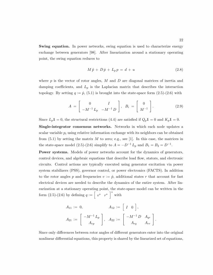
Swing equation. In power networks, swing equation is used to characterize energy
exchange between generators [98]. After linearization around a stationary operating
point, the swing equation reduces to
M p + D p + Lp p = d + u (2.8)
where p is the vector of rotor angles, M and D are diagonal matrices of inertia and
damping coefficients, and Lp is the Laplacian matrix that describes the interaction
topology. By setting q := p, (5.1) is brought into the state-space form (2.5)-(2.6) with
A =
[0 I
−M−1 Lp −M−1D
], Bi =
[0
M−1
]. (2.9)
Since Lp1 = 0, the structural restrictions (4.4) are satisfied if Qp1 = 0 and Kp1 = 0.
Single-integrator consensus networks. Networks in which each node updates a
scalar variable pi using relative information exchange with its neighbors can be obtained
from (5.1) by setting the matrix M to zero; e.g., see [1]. In this case, the matrices in
the state-space model (2.5)-(2.6) simplify to A = −D−1 Lp and B1 = B2 = D−1.
Power systems. Models of power networks account for the dynamics of generators,
control devices, and algebraic equations that describe load flow, stators, and electronic
circuits. Control actions are typically executed using generator excitation via power
system stabilizers (PSS), governor control, or power electronics (FACTS). In addition
to the rotor angles p and frequencies v := p, additional states r that account for fast
electrical devices are needed to describe the dynamics of the entire system. After lin-
earization at a stationary operating point, the state-space model can be written in the
form (2.5)-(2.6) by defining q :=[v∗ r∗
]∗with
A11 := 0, A12 :=[I 0
],
A21 :=
[−M−1 Lp
Arp
], A22 :=
[−M−1D Aqr
Arq Arr
].
Since only differences between rotor angles of different generators enter into the original
nonlinear differential equations, this property is shared by the linearized set of equations,

23
thereby implying A211 = 0. Furthermore, in the absence of the access to the absolute
rotor angle measurements both the matrix A in (2.6) and its closed-loop equivalent
in (2.5) have an eigenvalue at zero with the corresponding eigenvector[1∗ 0∗
]∗.
Such formulation has been recently utilized in [16].
Spatially-invariant systems
For systems with invariances and symmetries, transform techniques can be used to bring
a large-scale analysis and design problems into a parametrized family of smaller prob-
lems. One such class is given by spatially invariant systems that evolve over a discrete
spatially-periodic domain (e.g., a one-dimensional circle or a multi-dimensional torus).
In this case, the matrices in (2.5) are block circulant matrices and the application of the
discrete Fourier transform (DFT) in the spatially invariant directions brings them into a
block-diagonal form (2.2). As shown in [17], the optimal centralized controllers for spa-
tially invariant systems with quadratic performance indices are also spatially invariant;
thus, in the transformed domain they also take the block-diagonal form. Consequently,
determining the optimal centralized controller amounts to easily parallelizable task of
solving a sequence of smaller, fully-decoupled optimal control problems.
For spatially-invariant systems (2.5) with block-circulant matrices, the application
of DFT
x = T x, u = T u, d = T d, z = T z,
brings the closed-loop system (2.5) to the form (2.2) with block-diagonal matrices A,
B1, B2, C2, Q, R, and K. Here, T is the discrete Fourier matrix and the feedback gain
matrices are related via a linear transformation [38],
K = T (K) = T ∗K T.
2.1.3 Sparsity-promoting penalty functions
We briefly describe two classes of sparsity-promoting penalty functions. More sophisti-
cated penalties can also be introduced; see [16] for examples in power networks.

24
Elementwise sparsity. The weighted `1-norm,
g(K) :=∑
i, j
Wij |Kij | (2.10)
is a commonly used proxy for enhancing elementwise sparsity of the matrix K [99].
The non-negative weights Wij provide additional flexibility relative to the standard `1-
regularization. An iterative reweighting method was introduced in [99] to provide better
approximation of the non-convex cardinality function. In the mth iteration, the weights
Wij are set to be inversely proportional to the absolute value of Kij in the previous
iteration,
Wmij = 1/
(|Km−1
ij | + ε)
where 0 < ε� 1 guards against Kij = 0.
Block sparsity. By selecting g(K) to penalize the Frobenius norm of the ijth block
of the matrix K,
g(K) :=∑
i, j
Wij ‖Kij ‖F
sparsity can be enhanced at the level of submatrices [100]. In the iterative reweighting
algorithm, the absolute value should be replaced by the Frobenius norm of Kij
Wmij = 1/
(‖Km−1
ij ‖F + ε).
2.2 Class of convex problems
For an undirected consensus network in which each node updates a scalar value pi, we
next show that the sparsity-promoting optimal control problem can be formulated as
an SDP. The closed-loop system (2.5) with
A := −Lp, B1 = B2 := I, C2 = I, K := Lk

25
can be written asp = −(Lp + Lk) p + d
z =
[Q1/2
−R1/2 Lk
]p
(2.11)
where the symmetric positive semi-definite matrices Lp and Lk satisfy Lp 1 = 0, Lk 1 =
0. These two Laplacian matrices contain information about the interconnection struc-
ture of the open-loop system and the controller.
The `1-regularized H2 optimal control problem can be formulated as
minimizeLk
J(Lk) + γ ‖W ◦ Lk‖`1 . (2.12)
Here, ◦ denotes elementwise matrix multiplication and the solution to the algebraic
Lyapunov equation
(Lp + Lk)P + P (Lp + Lk) = Q + Lk RLk
determines the H2 of the closed-loop system, J(Lk) = trace (P ). It is readily shown
that the stability of (2.11) on the subspace 1⊥ amounts to positive-definiteness of the
matrix (Lp + Lk) on 1⊥. Under this condition, we can rewrite J(Lk) as
J(Lk) = trace((Lp + Lk)
† (Q+ Lk RLk))
=1
2trace
((Lp + Lk + 1
N 11T )−1(Q+ Lk RLk)
)
where (Lp + Lk)† denotes the Moore-Penrose pseudoinverse of (Lp + Lk), and cast the
sparsity-promoting optimal control problem (2.12) to an SDP via the Schur complement,
minimizeY,Z,Lk
1
2trace (Y ) + γ 1TZ 1
subject to
Y
[Q1/2
R1/2 Lk
]
( · )∗ Lp + Lk + 1N 11
T
� 0
Lk 1 = 0
−Z ≤ W ◦ Lk ≤ Z.
(2.13)
26
For small size problems, the resulting SDP formulation can be solved efficiently using
available SDP solvers.
In addition to the optimal edge design in undirected consensus networks, several
other classes of problems admit convex characterizations: a class of optimal synchroniza-
tion problems [11], optimal actuator/sensor selection [33, 34], symmetric modifications
of symmetric systems [19,35], and diagonal modifications of positive systems [28].
2.3 Design of controller structure
We next develop an algorithm, based on the Alternating Direction Method of Multipliers
(ADMM), to solve the sparsity-promoting optimal control problem (2.4),
minimizeK,K
J(K) + γ g(K)
subject to T (K) − K = 0.
As we describe next, the introduction of the linear constraint in (SP) in conjunction
with utilization of the ADMM algorithm allows us to exploit the respective structures
of the objective functions J and g in (2.4).
2.3.1 Structure design via ADMM
The structure of feedback gains that strike a balance between quadratic performance of
the system and sparsity of the controller is designed via ADMM. The ADMM algorithm
starts by introducing the augmented Lagrangian
Lρ(K,K,Λ) = J(K) + γ g(K) +⟨
Λ, T (K) − K⟩
+ρ
2
⟨T (K) − K, T (K) − K
⟩
where Λ is the Lagrange multiplier, ρ is a positive scalar, and 〈·, ·〉 is the standard inner
product between two matrices. Instead of minimizing the augmented Lagrangian jointly

27
with respect to K and K, ADMM uses a sequence of iterations [24],
Kk+1 = argminK
Lρ (K, Kk, Λk)
Kk+1 = argminK
Lρ (Kk+1, K, Λk)
Λk+1 = Λk + ρ (T (Kk+1) − Kk+1)
until primal and dual residuals are smaller than specified thresholds,
‖T (Kk+1)−Kk+1‖F ≤ εp, ‖Kk+1 −Kk‖F ≤ εd.
It is readily shown that K-minimization step amounts to the quadratically-augmented
minimization of J(K),
Kk+1 := argminK
(J(K) +
ρ
2‖T (K) − Hk‖2F
)
whereHk := Kk− (1/ρ) Λk. Similarly, using completion of squares, theK-minimization
problem can be brought into the following form
Kk+1 := argminK
(γ g(K) +
ρ
2‖K − V k‖2F
)
with V k := T (Kk+1) + (1/ρ) Λk. Thus, updating K requires computation of the
proximal operator of the function g.
K-minimization step
For elementwise sparsity, the objective function in the K-minimization step takes sep-
arable form, ∑
i, j
(γ Wij |Kij | +ρ
2
(Kij − V k
ij
)2),
and the update of K is obtained via convenient use of the soft-thresholding operator,
Kk+1ij =
(1 − a/|V kij |)V k
ij |V kij | > a
0 |V kij | ≤ a

28
where a := (γ/ρ)Wij . This analytical update of K is independent of the quadratic
performance index J . Similarly, for block sparsity, the minimizer is determined by
Kk+1ij =
(1 − a/‖V kij‖F )V k
ij ‖V kij‖F > a
0 ‖V kij‖F ≤ a
where Kij and Vij are the corresponding submatrices.
K-minimization step
Finding the solution to the K-minimization problem represents the biggest challenge
to solving the sparsity-promoting optimal control problem (2.4) via ADMM. In what
follows, we introduce two methods to solve the K-minimization problem: the Anderson-
Moore method and the proximal gradient method.
Anderson-Moore method. For the H2 optimal control problem (2.4), the optimality
conditions in the K-minimization step are given by
(A− B2KC2) X + X (A− B2KC2)∗ = −B1B∗1 (NC-X)
(A− B2KC2)∗P + P (A− B2KC2) = −(Q+ C∗2K∗R KC2) (NC-P)
2(RKC2 − B∗2P )XC∗2 + ρT †(T (K)−Hk) = 0 (NC-K)
where T † is the adjoint of the operator T ,
⟨K, T (K)
⟩=⟨T †(K), K
⟩.
The unknowns in this system of nonlinear matrix-valued equations are the feedback gain
K as well as the controllability and observability Gramians X and P of the closed-loop
system (2.2). These equations can have multiple solutions, each of which is a stationary
point of the K-minimization problem. In general, it is not known how many stationary
points exist or how to find all of them.
The Anderson-Moore method solves the above system of equations in an iterative
fashion. In each iteration, the algorithm starts with a stabilizing feedback matrix K
and solves two Lyapunov equations and one Sylvester equation. Specifically, it first

29
solves (NC-X) and (NC-P) for controllability and observability Gramians X and P
with K being fixed. Then the Sylvester equation (NC-K) is solved for K with X and
P being fixed.
For consensus and synchronization problems discussed in Section 2.1.2, we have
K = T (K) = K T ⇔ K = T †(K) = K T+
with TT+ = I. If the control weight R is given by a scaled version of the identity matrix
R = r I, r > 0
Sylvester equation (NC-K) can be explicitly solved for K,
K =(
2 B∗2 P X C∗2 + ρHk T+)(
2 r C2 X C∗2 + ρ I)−1
.
Following [21], we can show that the difference between two consecutive updates of
K forms a descent direction for
L(K) := J(K) +ρ
2‖ T (K) − Hk ‖2F .
In conjunction with backtracking, this can be used to determine step-size to guarantee
closed-loop stability and convergence to a stationary point of L(K).
Proximal gradient method. Proximal gradient method provides an alternative ap-
proach to solving the K-minimization step. It is based on a simple quadratic approxi-
mation of the quadratic objective function J(K) around current inner iterate Km,
J(K) ≈ J(Km) + 〈∇J(Km), K − Km〉+1
2αm‖K − Km‖2F
where αm denotes the step-size and
∇J(Km) = 2 (R Km C2 − B∗2 Pm) Xm C∗2 .

30
Using completion of squares, the K-minimization step can be written as
Km+1 = argminK
(1
2αm‖ K −
(Km − αm∇J(Km)
)‖2F +
ρ
2‖T (K)−Hk‖2F
)
and the optimality condition is given by
1
αm
(K −
(Km − αm∇J(Km)
))+ ρ T †
(T (K)−Hk
)= 0 (2.14)
For consensus and synchronization networks, T (K) = KT , and we have an explicit
update for K,
Km+1 =1
1 + αm ρ
(Km − αm∇J(Km) + αm ρH
k T+)
The proximal gradient algorithm converge with rate O(1/m) if αm is smaller than the
reciprocal of the Lipschitz constant of ∇J [101]. Since the Lipschitz constant is difficult
to determine explicitly, we adjust αm via backtracking procedure that we describe next.
Furthermore, to enhance the speed of convergence, we initialize the step-size using the
Barzilai-Borwein (BB) method [102],
α0m =
‖ Km − Km−1‖2F⟨Km−1 − Km,∇J(Km−1)−∇J(Km)
⟩ ,
The BB method approximates the Hessian with a scaled version of the identity matrix
and it represents an effective heuristics for improving convergence rate. The initial step-
size α0m is adjusted via backtracking to guarantee closed-loop stability and to make sure
that,
J(Km+1) ≤ J(Km) +⟨∇J(Km), Km+1 − Km
⟩+
1
2αm‖Km+1 − Km‖2F .
The proximal gradient method terminates when
‖∇L(Km)‖F ≤ εK .
31
Remark 1. For spatially-invariant systems, the computational complexity of each K-
minimization step is O(Nn3s). Here, N denotes the number of subsystems and ns is the
number of states in each subsystem. This should be compared and contrasted to O(n3)
complexity, with n = Nns, for systems without spatially-invariant structure.
2.3.2 Polishing step
After having identified the sparsity pattern Sp via ADMM, we optimize the network
performance over the identified structure,
minimizeK
J(K)
subject to T (K) ∈ Sp.(2.15)
We fix the sparsity pattern of K and solve the optimal control problem (2.15) via an
ADMM algorithm, where the K-minimization step is the same as in Section 2.3.1 while
the K-minimization step is computed by projecting the new K = KT onto the convex
set Sp. This polishing step is used to further improve performance of sparse feedback
gains resulting from the structure design step.
2.4 Case study: synchronization network
Twenty nodes in an undirected disconnected network shown in Fig. 2.1 are randomly
distributed in a unit square. The nodes form three clusters and the network dynamics
are described by the swing equation (5.1). The state-space model is given by (2.5) with
C2 = I and the matrices A, B1, and B2 determined by (2.9). The graph Laplacian Lp is
obtained based on the proximity of the nodes: two nodes are connected if their distance
is not greater than 0.25. The control objective is to minimize performance metric that
penalizes angular kinetic energy and the mean square deviation from the angle average.
Information exchange links in the controller graph that result from elementwise
sparsity-promoting regularizer with iterative re-weighting are illustrated in Fig. 2.2.
Since local frequency measurements are readily available, the diagonal elements of the
frequency feedback gains are not penalized in the function g. The red lines mark the

32
Figure 2.1: Topology of a disconnected plant network with 3 clusters and 20 nodes.
identified communication links (of either the rotational angles or the frequencies) be-
tween the nodes. As we increase γ, the controller graph becomes sparser. For γ = 1,
there are only two long-range links that connect two small clusters to the large cluster
of nodes. The controller makes the original disconnected graph connected by adding
links between different clusters, thereby guaranteeing synchronization and optimizing
the desired performance metric.
The structure of the feedback gain K for γ = 1 is shown in Fig. 2.3. The blue
dots denote local feedback gains and the red dots identify information that needs to be
communicated between different nodes. Since the frequency feedback gain matrix is di-
agonal, only local frequency measurements are required to form the control action. The
two red dots correspond to the two red long-range links in Fig. 2.2d and they indicate
that the controllers of the two furthest nodes require access to the angle measurements
of the node in the center of the domain. Dropping any of these two links would yield a
disconnected closed-loop network and synchronization would not be achieved.
Compared to the optimal centralized controller, the sparse controller with structure
shown in Fig. 2.2d compromises performance by 8.81%; see Fig. 2.4. In contrast, the
sparse controller in Fig. 2.2c has five additional long-range links and degrades perfor-
mance by only 3.4%.
Finally, for each value of the regularization parameter γ we compare and contrast
performance of the controller with the sparsity pattern shown in Fig. 2.3 with a heuris-
tic strategy that has the same sparsity level. The diagonal elements of the frequency
feedback gain are always non-zero and sparsity pattern for the rest of the elements is

33
(a) γ = 0.0010 (b) γ = 0.0072
(c) γ = 0.0596 (d) γ = 1
Figure 2.2: Topology of controller network for different values of γ. Edges in thecontroller network are marked with red lines.
Figure 2.3: Sparsity pattern of K for γ = 1.
randomly selected. For each sparsity level, we randomly select 100 off-diagonal patterns
and optimize feedback gains over the fixed structure. Figure 2.5 compares the aver-
age closed-loop performance degradation of this heuristic strategy to our method. For
each sparsity level, our approach yields smaller performance loss and offers significant
advantages for sparser control architectures (i.e., larger values of γ).

34
(J − Jc) /Jc card (K) /card (Kc)
10−3 10−2 10−1 1000
2
4
6
8
10
γ
perc
ent
10−3 10−2 10−1 1000
10
20
30
40
50
γ
perc
ent
Figure 2.4: Performance vs sparsity comparison with respect to the optimal centralizedcontroller Kc for 50 logarithmically-spaced points γ ∈ [ 10−3 , 1 ].
(J − Jc) /Jc
10−3 10−2 10−1 1000
5
10
15
20
25
30
γ
perc
ent
Figure 2.5: Performance degradation comparison of K resulting from our framework(dots) to the average of 100 feedback matrices of random sparsity patterns with samesparsity level for each γ.
2.5 Concluding remarks
In this section, we have considered a regularized version of the standard H2 optimal
control problem where the regularization term serves as a proxy for inducing sparsity.
We consider a class of systems in which state-space representation is not cast in the set of
coordinates in which it is desired to enhance sparsity. This setup arises in systems with
invariances and symmetries as well as in consensus and synchronization networks. We
achieve desired performance with fewer communication links in the controller network
by promoting sparsity of the feedback gain matrix. Alternating direction method of
multipliers allows for performance and sparsity requirements to be expressed in different

35
set of coordinates and facilitates efficient computation. A synchronization network
is provided as an illustrative example to demonstrate the value of our developments.
Recently, our generalized sparsity-promoting optimal control framework was used to
suppress inter-area oscillations in power networks [16].
Chapter 3
Sparsity-promoting optimal
control of systems with
invariances and symmetries
We take advantage of system invariances and symmetries to gain convexity and com-
putational advantage in regularized H2 and H∞ optimal control problems. For systems
with symmetric dynamic matrices, the problem of minimizing the H2 or H∞ perfor-
mance of the closed-loop system can be cast as a convex optimization problem. Al-
though the assumption of symmetry is restrictive, studying the symmetric component
of a general system’s dynamic matrices provides bounds on the H2 and H∞ perfor-
mance of the original system. Furthermore, we show that for certain classes of systems,
block-diagonalization of the system matrices can bring the regularized optimal control
problems into forms amenable to efficient computation via distributed algorithms.One
such class of systems is spatially-invariant systems, whose dynamic matrices are circu-
lant and therefore block-diagonalizable by the discrete Fourier transform [103].
36

37
3.1 Problem formulation
We consider the class of systems,
x = (A − K(v))x + Bd
z =
[C
R(v)
]x
(3.1)
where v ∈ Rm is a design parameter, K(·) : Rm → Rn×n is a linear operator, x(t) ∈Rn is the state vector, C is mapping from the state to a regulated output, R(v) is a
mapping from the state to a measure of control effort, d(t) ∈ Rp is a white stochastic
disturbance with E (d(t1) dT (t2)) = Iδ(t1 − t2), and E is the expectation operator.
Taking v = vec(F ), K(v) = B2F and R(v) = R1/2F where R � 0 ∈ Rp×p, F ∈ Rp×n,
and B2 ∈ Rn×p yields the traditional state feedback control problem. We consider v to
be constant in time.
Our objective is to design a stabilizing v that solves the regularized optimal control
problem,
minimizev
J(v) + g(v)
subject to A − K(v) Hurwitz(3.2)
where J(v) is a performance metric, taken to be either the closed loop H2 or H∞ norm,
and g(v) can be any convex function of v. The H2 performance, which we denote by
J2(v), is a measure of the variance amplification from the disturbances d to the regulated
output z in system (3.1),
J2(v) := limt→∞
E(zT (t) z(t)
)
which can be computed by
J2(v) = trace(X(CTC + RT (v)R(v))
)
where X is the controllability gramian
(A − K(v))X + X (A − K(v))T + BBT = 0.

38
The H∞ performance metric, which we denote by J∞(v), is the maximum induced L2
gain from d to z in system (3.1),
J∞(v) := sup‖d‖L2
≤1
‖z‖L2‖d‖L2
,
where the L2 norm of a signal f is defined as,
‖f‖2L2 :=
∫ ∞
0f2(t) dt.
This performance metric corresponds to the peak of the frequency response,
J∞(v) = supω
σmax
(C (jωI − (A + K(v) ) )−1B
).
The unregularized H2 and H∞-optimal linear state feedback problems can be cast in a
convex form via a suitable change of coordinates; however, this change of coordinates
does not preserve the structure of the design variable v.
For many applications, v has physical significance and penalizing it directly via g(v)
is desirable. For example, a quadratic penalty, ‖v‖22, would limit the magnitude of v,
and an `1 penalty, ‖v‖1 :=∑
i |vi|, would promote sparsity.
Many structured optimal control problems can be cast in the form of (3.2). For
example, structured state feedback problems have been extensively studied with partic-
ular applications to consensus networks and power systems [16, 21, 30, 81, 82, 104, 105].
Two other applications are given below.
3.1.1 Applications
Design of edges in networks
The problem of adding undirected edges to an existing network can be cast in this
problem form. The dynamics are,
x = −(L + E diag(v)ET
)x + d

39
where L is a directed graph Laplacian which contains information about how the nodes
are connected, E contains information about the locations of potential added edges,
and K(v) := E diag(v)ET is a diagonal matrix of added edge weights [106]. Taking the
regularizer to be the `1 norm g(v) =∑
i |xi| would limit the number of edges added to
the network.
Combination drug therapy design for HIV treatment
The problem of designing drug dosages for treating HIV [107,108] can be cast as,
x =
(A −
m∑
k=1
vkDk
)x + d.
Here, the elements of x represent populations of HIV mutants. The diagonal elements of
A represent each mutant’s replication rate and the off diagonal elements of A represent
the probability of mutation from one mutant to another. The components of the vector
v are dosages of different drugs, where Dk is a diagonal matrix containing information
about how efficiently drug k kills each HIV mutant. Here, quadratic regularization
g(v) = ‖v‖22 would limit the dose of the drugs prescribed and `1 regularization g(v) =∑
i |xi| would limit the amount of drugs prescribed.
3.2 Symmetric system design
One class of system for which J2(v) and J∞(v) are convex arises when B = C = I,
and A and K(v) are symmetric matrices. Although this assumption seems restrictive,
studying such systems can inform the design of structured controllers for more general
classes of systems.
Any matrix A can be decomposed into its symmetric As =1
2(A+AT ) and antisym-
metric Aa =1
2(A−AT ) components. The system which corresponds to the symmetric
components of the general system (3.1),
x = (As − Ks(v) ) x + d (3.3)

40
where Ks(v) =1
2(K(v) +KT (v)) reveals interesting characteristics of the original sys-
tem.
In this section, we first show the convex formulations that correspond to the optimal
H2 and H∞ design of symmetric systems. We then establish stability guarantees and
performance bounds for applying controllers designed by solving the convex problem of
regularized optimal control on the symmetric system (3.3) to the original system (3.1).
Finally, we use perturbation analysis to show that the symmetric system is a high fidelity
approximation for systems which are dominated by the symmetric component.
3.2.1 Convex optimal control for symmetric systems
Although more general symmetric systems can be cast as convex problems, here we
assume B = C = I and R(v) = 0 to facilitate the transition to the discussion of spectral
properties and performance bounds.
H2-optimal control
When As = ATs is symmetric, the controllability Gramian of system (3.3) can be explic-
itly expressed as,
Xs = −1
2(As − Ks(v) )−1
and, by taking a Schur complement, the regularized optimal H2 control problem can be
cast in a convex function of v and an auxiliary variable Θ,
minimizev,Θ
1
2trace(Θ) + g(v)
subject to
[Θ I
I −As +Ks(v)
]� 0.
(3.4)
The matrix As−Ks(v) is always invariable when it is Hurwitz. We note the structured
LQR problem (i.e., R(v) = R1/2Ks(v)) for symmetric systems can also be expressed as
an SDP by taking the Schur complement of Ks(v)RKs(v).

41
H∞-optimal control
The peak of the frequency response of a symmetric system occurs at ω = 0.
Proposition 1. For a system (3.3) with symmetric dynamics, the disturbance that
achieves the maximum induced L2 amplification corresponds to the constant signal d(t) =
v where v is the right principal singular vector of A−1.
Proof. A symmetric matrix can be diagonalized as, As = UΛUT where Λ is a diagonal
matrix with the eigenvalues of As on the main diagonal and the columns of U contain
the corresponding eigenvectors. For such a matrix,
(jωI − As)−1 = U diag
{1
jω − λi
}UT .
It is clear that ω = 0 maximizes the singular values of the above matrix. Thus, the H∞norm of (3.3) can be characterized by σmax
(−(As − K(v))−1
).
The H∞-optimal control problem for symmetric systems can therefore be expressed
as,
minimizev,Θ
σmax(Θ) + g(v)
subject to
[Θ I
I −As +Ks(v)
]� 0.
(3.5)
As we show in the next subsection, this convex problem can be used for structured
H∞ control design. This is particularly advantageous because many of the existing
algorithms for general structured H2 control cannot be extended to the structured H∞problem.
3.2.2 Stability and performance guarantees
Stability of the symmetric system (3.3) implies stability of the corresponding original
system (3.1).
Lemma 2. [35, Lemma 1] Let the symmetric part of A, As := (A+AT )/2, be Hurwitz.
Then, A is Hurwitz.
Remark 2. This is not a necessary condition; A may be Hurwitz even if As is not.

42
Performance guarantees
The H2 and H∞ norms of the symmetric system are upper bounds on the H2 and H∞norms of the original system.
Proposition 3. [35, Cor. 3] When the systems (3.1) and (3.3) are stable, the H2 norm
of the general system (3.1) is bounded from above by the H2 norm of the symmetric
system (3.3).
We show that an analagous bound holds for the H∞.
Proposition 4. When the systems (3.1) and (3.3) are stable, the H∞ norm of the gen-
eral system (3.1) is bounded from above by the H∞ norm of the symmetric system (3.3).
Proof. From the bounded real lemma [109], the H∞ norm of the general system (3.1)
is less than γ if there exists a P � 0 such that,
ATP + P A + I + γ−2 P 2 ≺ 0.
From Proposition 1, for the symmetric system (3.3), γ > σmax(A−1s ). Taking P = γI for
any γ > σmax(A−1s ) and substituting it into the above linear matrix inequality (LMI)
applied to the symmetric system (3.3) yields,
2 γ As + 2 I ≺ 0.
Since As is Hurwitz, As ≺ 0. Since γ > −λmax(A−1s ), γ−1 < −λmin(As), so As ≺ −γ−1I.
Therefore the LMI is satisfied. Since Aa = −ATa , setting P = γI implies,
ATP + P A = 2 γ As
therefore substituting P into the bounded real lemma LMI for the general system (3.1),
where A = As +Aa, yields,
ATP + P A + I + γ−2 P 2 = 2 γ As + 2 I ≺ 0.

43
3.2.3 Approximation bounds
In addition to being an upper bound, the H2 and H∞ norms of the symmetric (3.3) and
full (3.1) systems are close when A is dominated by the symmetric component.
Proposition 5. [35, Prop. 4] Let An be a normal matrix. The O(ε) correction to the
H2 norm of the system
x = An x + d
from an O(ε) antisymmetric perturbation Aa is zero.
We show that a similar property holds for the H∞ norm.
Proposition 6. Let As be a symmetric matrix. The O(ε) correction to the H∞ norm
of the system
x = As x + d
from an O(ε) antisymmetric perturbation Aa is zero.
Proof. From Proposition 1, theH∞ norm of the symmetric system is given by σmax(−A−1s ).
The maximum singular value of a matrix is equivalent to,
σmax(X) = sup‖v‖2≤1,‖w‖2≤1
vTXw.
Since As is symmetric, w = v. Taking an O(ε) antisymmetric perturbation Aa to the
above expression,
σmax (−(As + εAa)−1) ≈ −vTA−1
s v + ε vTA−1s AaA
−1s v.
Since Aa is antisymmetric,⟨A−1s vvTA−1
s , Aa⟩
= 0.
3.3 Computational advantages for structured problems
Structured control is often of interest for large-scale systems. As such, the computa-
tional scaling of algorithms used to compute optimal controllers is very important. In
this section, we identify a class of systems which are amenable to scalable distributed
algorithms.

44
When A and K(v) are always simultaneously block-diagonalizable, the dynamics of
the system can be expressed as the sum of independent subsystems. Define x := Px
and let P be a unitary matrix such that,
˙x = (A + K(v))x
where
A := P AP T , K(v) := P K(v)P T ,
and, for any choice of v, A + K(v) = blkdiag{A11 + K11, · · · , ANN + KNN} is block-
diagonal with N blocks of size n× n each.
For problems of this form, computing optimal control strategies is much more effi-
cient in the x coordinates because the majority of the computational burden in solving
problems (3.4) and (3.5) comes from the nN×nN LMI constraint involved in minimizing
the performance metrics J2(v) or J∞(v).
For this class of system, the H2-optimal control problem (3.4) can be expressed as,
minimizev,Θi
1
2
∑
i
trace(Θi) + g(v)
subject to
[Θi I
I −(As)ii + (Ks(v))ii
]� 0.
(3.6)
which is an SDP with N separate n × n LMI blocks. Since SDPs scale with the sixth
power of the LMI blocks, solving this reformulation scales with n6 as opposed to n6N6.
Analogously, the structured H∞-optimal control problem (3.5) can be cast as,
minimizev,Θi
maxi
(σmax(Θi)) + g(v)
subject to
[Θi I
I (As)ii − (Ks(v))ii
]� 0.
(3.7)
One important class of system which satisfies these assumptions is spatially-invariant
systems. This structure was used in [38] to develop efficient techniques for sparse feed-
back synthesis.

45
3.3.1 Spatially-invariant systems
Spatially-invariant systems have a block-circulant structure which is block-diagonalizable
by a Discrete Fourier Transform (DFT). A spatially-invariant system can be represented
by N subsystems with n states each. The state vector x ∈ RnN is composed of N sub-
vectors xi ∈ Rn which denotes the state of the subsystem. The matrix A ∈ RnN×nN is
block-circulant with blocks of the size n× n. For example, when N = 3,
A =
A0 A1 A−1
A−1 A0 A1
A1 A−1 A0
where the blocks {A0, A−1, A1} ∈ Rn×n.
It was shown in [17] that the optimal feedback controller for a spatially-invariant
system is itself spatially-invariant. Assuming that the optimal sparse feedback con-
troller is also spatially-invariant is equivalent to assuming that K(v) is block-circulant.
Block circulant matrices are block-diagonalizable by the appropriate DFT. Let the block
Fourier matrix be
Φ := ΦN ⊗ In,
where In is the n × n identity matrix, ΦN is the N ×N discrete Fourier transform
matrix, and ⊗ represents the Kronecker product. By introducing the change of variables
x := Φx, where
x =[xT1 · · · xTN
]T,
and xi ∈ Rn, the original system’s dynamics can be expressed as N independent n× nsubsystems,
A =
A11
A22
A33
Consequently, the optimal structured control problems (3.4) and (3.5) can be cast
as (3.6) and (3.7), which are more amenable to efficient computations.

46
3.4 Examples
3.4.1 Directed Consensus Network
In this example, we illustrate the utility of the approach described in Section 3.2. Con-
sider the network dynamics given by a directed network as described in Section 3.1.1,
x = −(L + E diag(v)ET )x
where L is a directed graph Laplacian, K(v) = Ediag(v)ET represents the addition
of undirected links, v is a vector that contains weights of these added links, and the
incidence matrix E describes which edges may be added or altered. The regularization
on v is given by,
g(v) = ‖v‖22 + γ∑
i
|vi|
where the quadratic term limits the size of the edge weights, the `1 norm promotes
sparsity of added links, and γ > 0 parametrizes the importance of sparsity.
For this concrete example, the network topology is given by Figure 3.1. The potential
added edges can connect the following pairs of nodes: (1) − (2), (1) − (3), (1) − (5),
(1)− (6), (2)− (5), (2)− (6), (3)− (6), and (4)− (5).
Controllers were designed by solving problems (3.4) and (3.5) for the symmetric
version of the network over 50 log-distributed values of γ ∈ [10−4, 1]. The closed-loop
H2 and H∞ norms obtained by applying these controllers to the symmetric and original
systems are shown in Fig. 3.2. Figure 3.1 also shows which edges were added for γ = 1.
3.4.2 Swift-Hohenberg Equation
Here we illustrate the utility of the block-diagonalization we describe in Section 3.3.
Consider a particular realization of the Swift-Hohenberg equation [110],
∂tψ(t, x) = β ψ(t, x) − (1 + ∂xx)2 ψ(t, x) + v(x)ψ(t, x)
where β ∈ R, and ψ(t, ·), v(·) ∈ L2(−∞,∞), and v(x) is a spatially-invariant feedback
controller which is to be designed. A finite dimensional approximation of this system
can be obtained by using the differentiation suite from [111] to discretize the problem

47
1
23
5
4
6
Figure 3.1: Directed network (black solid arrows) with added undirected edges ( reddashed arrows). Both the H2 and H∞ optimal structured control problems yielded thesame set of added edges. In addition to these edges, the controllers tuned the weightsof the edges (1)− (3) and (1)− (5).
into N points and approximating the infinite domain with periodic boundary conditions
over the domain L2[0, 2π]. A sparse H2 feedback controller v(x) can then be identified
by solving problem (3.4).
We contrast this method with the approach we advocate in Section 3.3, where we
use the DFT to decompose the system into N first-order systems corresponding to
eigenfunctions of the Swift-Hohenberg equation and solve problem (3.6).
The state vector takes the form of ψ(x) evaluated at grid points in x where the
dynamics are given by,
ψ = (A − V )ψ
where, A = βI − (I +D2)2. Here D is a discrete differentiation matrix from [111], and
V is the circulant state feedback matrix.
Using the DFT over x, the Swift-Hohenberg equation can be expressed as a set of
independent first-order systems,
˙ψx = (ax − vx)ψx
where ax := β− (1−κ2x)2, and the new coordinates are ψ := Pψ, P is the DFT matrix,
κx is the wavenumber (spatial frequency), and v represents V in the Fourier space; i.e.,
V = P Tdiag(v)P .

48
Figure 3.2: H2 and H∞ performance of the closed-loop symmetric system and theoriginal system subject to a controller designed at various values of γ.
We take the regularization term to be
g(v) = ‖V ‖2F + γ‖V ‖1
where ‖X‖1 :=∑
ij |Xij | is the elementwise `1 norm and γ is a parameter which specifies
the emphasis on sparsity relative to performance.
For the H2 problem, the regularized optimal control problem is of the form of (3.4)
with Ks(v) = V and V is circulant. In that formulation, the problem is an SDP with
one N × N LMI block. In the Fourier space, the problem can be expressed as (3.6),
which takes the particular form,
minimizev
1
2
∑ 1
−ax + vx+ g
(P Tdiag(v)P
)
subject to − ax + vx ≥ 0
which does not require the large SDP constraints in (3.4).
We solved the regularized H2 optimal control problem by solving the general formu-
lation (3.4) and the more efficient formulation (3.6) for β = 0.1, γ = 1 and N varying
from 5 to 51 using CVX, a general purpose convex optimization solver [112].
Taking advantage of spatial invariance yields a significant computational advantage,
as can be seen in Figure 3.3. Although both expressions of the problem yield the same

49
solution, solving the realization in (3.6) is much faster and allows us to examine much
larger problem dimensions. In Figure 3.4, we show the spatially-invariant feedback
controller for one point in the domain, i.e., one row of V , computed for N = 101 at
γ = 0, γ = 0.1, and γ = 10..
Figure 3.3: Computation time for the general formulation (3.4) (blue ◦) and that whichtakes advantage of spatial invariance (3.6) ( red ∗).
Figure 3.4: Feedback gain v(x) for the node at position x = 0, computed with N = 51and γ = 0 (black solid), γ = 0.1 (blue dashed), and γ = 10 ( red dotted).

50
3.5 Concluding remarks
We have provided a convex methodology for structured H2 and H∞ controller design
and a procedure to gain computational efficiency for spatially invariant systems and
problems with similar forms. Ongoing work will focus on deriving a bound on the
error between a general linear system and the system corresponding to its symmetric
component.

Part II
Wide-area control of power
systems
51

Chapter 4
Decentralized optimal control of
inter-area oscillations
Local and inter-area oscillations in bulk power systems are typically identified using
spatial profiles of poorly damped modes, and they are mitigated via carefully tuned
decentralized controllers. In this chapter, we employ non-modal tools to analyze and
control inter-area oscillations. Our input-output analysis examines power spectral den-
sity and variance amplification of stochastically forced systems and offers new insights
relative to modal approaches. To improve upon the limitations of conventional wide-
area control strategies, we also study the problem of signal selection and optimal design
of sparse and block-sparse wide-area controllers. In our design, we preserve rotational
symmetry of the power system by allowing only relative angle measurements in the
distributed controllers. For the IEEE 39 New England model, we examine performance
tradeoffs and robustness of different control architectures and show that optimal re-
tuning of fully-decentralized control strategies can effectively guard against local and
inter-area oscillations.
4.1 Modeling and control preliminaries
A power network is described by a nonlinear system of differential-algebraic equations.
Differential equations govern the dynamics of generators and their controllers, and the
algebraic equations describe quasi-stationary load flow and circuitry of generators and
52

53
power electronics [98]. A linearization around a stationary operating point and elimi-
nation of the algebraic equations yield a linearized state-space model
x = Ax + B1 d + B2 u. (4.1)
Here, x(t) ∈ Rn is the state, u(t) ∈ Rm is the generator excitation control input, and
d(t) ∈ Rp is the stochastic disturbance which may arise from power imbalance and
uncertain load demands [98]. For example, the choice B1 = B2 can be used to quantify
and mitigate the impact of noisy or lossy communication among spatially distributed
controllers [15].
4.1.1 Swing equations
The dominant electro-mechanical dynamics of a power system are given by the linearized
swing equations [98],
Mi θi + Di θi +∑
jLij (θi − θj) = 0.
These equations are obtained by neglecting fast electrical dynamics and eliminating the
algebraic load flow. Here, θi and θi are the rotor angle and frequency of generator i, Mi
and Di are the generator inertia and damping coefficients, and Lij is the (i, j) element
of the network susceptance matrix indicating the interactions between generators i and
j [15]. Even though the swing equations do not fully capture complexity of power
systems, they nicely illustrate the causes of inter-area oscillations: Inter-area oscillations
originate from sparse links between densely connected groups of generators (so-called
areas). These areas can be aggregated into coherent groups of machines which swing
relative to each other using the slow coherency theory [113, 114]. Our goal is to design
wide-area controllers to suppress inter-area oscillations.
4.1.2 Problem formulation
Under a linear state-feedback,
u = −Kx

54
the closed-loop system takes the form
x = (A − B2K)x + B1 d
z =
[z1
z2
]=
[Q1/2
−R1/2K
]x
(4.2)
where z is a performance output with state and control weights Q and R. We choose R
to be the identity matrix and a state objective that quantifies a desired potential energy
and the kinetic energy stored in the electro-mechanical dynamics,
xTQx = θTQθ θ +1
2θTM θ.
Here, M = diag (Mi) is the inertia matrix and the matrix Qθ penalizes the deviation of
angles from their average θ(t) := (1/N)1T θ(t),
Qθ = I − (1/N)11T (4.3)
where N is the number of generators and 1 is the vector of all ones. In a power system
without a slack bus, the generator rotor angles are only defined in a relative frame of
reference, as can be observed in the swing equations. Thus, they can be rotated by a
uniform amount without changing the fundamental dynamics (4.1). We preserve this
rotational symmetry and study problems in which only differences between the compo-
nents of the vector θ(t) ∈ RN enter into (4.2). As a result of the rotational symmetry,
both the open-loop A-matrix and the performance weight Qθ have an eigenvalue at zero
which characterizes the mean of all rotor angles.
By expressing the state vector as
x(t) :=
[θ(t)
r(t)
]∈ Rn
where r(t) ∈ Rn−N represents the rotor frequencies and additional states that account
for fast electrical dynamics, we arrive at the structural constraints on the matrices

55
in (4.2),
A
[1
0
]= 0, Qθ 1 = 0, K
[1
0
]= 0.
In earlier work [14,15], we have removed this rotational symmetry by adding a small
regularization term to the diagonal elements of the matrix Qθ. This has resulted in a
controller that requires the use of absolute angle measurements to stabilize the average
rotor angle. Such a regularization induces a slack bus (a reference generator with a fixed
angle) and thereby alters the structure of the original power system.
We preserve the natural rotational symmetry by restricting our attention to rela-
tive angle measurements. This requirement implies that the average rotor angle has
to remain invariant under the state feedback u = −Kx. To cope with these addi-
tional structural constraints, the sparsity-promoting approach of [21] has been recently
augmented in [30].
To eliminate the average-mode θ from (4.2) we introduce the following coordinate
transformation [30],
x =
[θ
r
]=
[U 0
0 I
]
︸ ︷︷ ︸T
ξ +
[1
0
]θ (4.4)
where the columns of the matrix U ∈ RN×(N−1) form an orthonormal basis that is
orthogonal to span (1). For example, these columns can be obtained from the (N − 1)
eigenvectors of the matrix Qθ in (4.3) that correspond to the non-zero eigenvalues. In
the new set of coordinates, ξ(t) = T Tx(t) ∈ Rn−1, the closed-loop system takes the form
ξ = (A − B2F ) ξ + B1 d
z =
[z1
z2
]=
[Q1/2
−R1/2 F
]ξ
(4.5)
where
A := T TAT, Bi := T TBi, Q1/2 := Q1/2 T.
The feedback matrices K and F (in the original x and new ξ coordinates, respectively)

56
are related by
F = K T ⇔ K = F T T .
Because of a marginally stable average mode, the matrix A in (4.2) is not Hurwitz.
The coordinate transformation (4.4) eliminates the average angle θ from (4.2), thereby
leading to (5.15) with Hurwitz A. In the presence of stochastic disturbances, θ(t) drifts
in a random walk. Since θ is not observable from the performance output z (which
quantifies the mean-square deviation from angle average, kinetic energy, and control
effort), z has a finite steady-state variance. This variance is determined by the square
of the H2 norm of system (5.15).
4.2 Input-output analysis
The conventional analysis of inter-area oscillations in power systems is based on spatial
profiles of eigenvectors and participation factors of poorly damped modes. Similarly,
traditional control design builds on a modal perspective [42, 43]. In systems with non-
normal A-matrices, modal analysis may lead to misleading conclusions about transient
responses, amplification of disturbances, and robustness margins [115–117]. Non-normal
matrices are common in power systems; such matrices do not have orthogonal eigenvec-
tors and they cannot be diagonalized via unitary coordinate transformations.
In what follows, we utilize an approach that offers additional and complementary
insights to modal analysis. This approach is based on the input-output analysis, where
the input d is the source of excitation and the output z is the quantity that we care
about. In stochastically forced systems, input-output analysis amounts to the study
of power spectral density and variance amplification. Our approach builds on the H2
paradigm [12], which analyzes and mitigates amplification of white stochastic distur-
bances.
4.2.1 Power spectral density and variance amplification
We next provide a brief overview of the power spectral density and variance amplifi-
cation analyses of linear dynamical systems. Let H(jω) denote the frequency response

57
of (5.15),
z(jω) = H(jω) d(jω).
The Hilbert-Schmidt norm determines the power spectral density of H(jω),
‖H(jω)‖2HS = trace (H(jω)H∗(jω)) =∑
σ2i (H(jω))
where σi’s are the singular values of the matrix H(jω). The H2 norm quantifies the
steady-state variance (energy) of the output z of stochastically forced system (5.15). It
is obtained by integrating the power spectral density over all frequencies [12],
‖H‖22 := limt→∞
E(zT (t) z(t)
)=
1
2π
∫ ∞
−∞‖H(jω)‖2HS dω
where E is the expectation operator. Equivalently, the matrix solution X to the Lya-
punov equation,
(A − B2F )X + X (A − B2F )T = −B1BT1
can be used to compute the H2 norm [12],
J(F ) := ‖H‖22 = trace(X (Q + F TRF )
)
= trace (Z1) + trace (Z2) .(4.6)
Here, X is the steady-state covariance matrix of the state ξ in (5.15), X := limt→∞E (ξ(t) ξT (t)),
and the covariance matrices of the outputs z1 and z2 are determined by
Z1 := limt→∞
E(z1(t) zT1 (t)
)= Q1/2X Q1/2
Z2 := limt→∞
E(z2(t) zT2 (t)
)= R1/2F X F TR1/2.
Note that trace (Z1) and trace (Z2) quantify the system’s kinetic and potential energy
and the control effort, respectively. In particular, the eigenvalue decomposition of the
matrix Z1,
Z1 =∑
λi yi yTi

58
determines contribution of different orthogonal modes yi to the kinetic and potential
energy in statistical steady-state. The total energy is given by trace (Z1), i.e., the
sum of the eigenvalues λi of the covariance matrix Z1. Each mode yi contributes λi
to the variance amplification and the spatial structure of the most energetic mode is
determined by the principal eigenvector y1 of the matrix Z1.
4.3 Sparse and block-sparse optimal control
In this section, we study the problem of optimal signal selection and optimal design
of wide-area controllers. We approach this problem by invoking sparsity-promoting
versions of the standard H2 optimal control formulation. We build on the framework
developed in [19–21, 30] which is aimed at finding a state feedback that simultane-
ously optimizes the closed-loop variance and induces a sparse control architecture. This
is accomplished by introducing additional regularization terms to the optimal control
problem. These serve as proxies for penalizing the number of communication links in
the wide-area controller, thereby inducing a sparse control architecture.
4.3.1 Elementwise sparsity
As shown in Section 4.2, the H2 norm of system (5.15) is determined by (4.6). While
the H2 performance is expressed in terms of the feedback matrix F in the new set of
coordinates, it is necessary to enhance sparsity of the feedback matrix K in the physical
domain. A desired tradeoff between the system’s performance and the sparsity of K is
achieved by solving the regularized optimal control problem [30],
minimizeF,K
J(F ) + γ g(K)
subject to F T T − K = 0.(4.7)
The regularization term in (SP) is given by the weighted `1-norm of K,
g(K) :=∑
i, j
Wij |Kij |

59
which is an effective proxy for inducing elementwise sparsity [99]. The weights Wij ’s
are updated iteratively using the solution to (SP) from the previous iteration; see [99]
for details. In (SP), γ is a fixed positive scalar that characterizes the emphasis on
the sparsity level of the feedback matrix K. A larger value of γ introduces a sparser
feedback gain K at the expense of degrading the closed-loop performance.
We solve the optimal control problem (SP) for different values of the positive regu-
larization parameter γ via the alternating direction method of multipliers; see [21, 30]
for algorithmic details. This allows us to identify a parameterized family of distributed
control architectures that strikes an optimal balance between competing performance
and sparsity requirements.
4.3.2 Block sparsity
In power systems, only rotor angle differences enter into the dynamics and information
about absolute angles is not available. It is thus advantageous to treat rotor angles
separately from the remaining states in the control design. We partition K conformably
with the partition of the state vector x,
K =[Kθ Kr
]
where Kθ and Kr are the feedback gains acting on the rotor angles and the remaining
states, respectively.
The actuators in wide-area control range from Power System Stabilizers (PSSs) to
power electronics devices (FACTS) to HVDC links. While our design methodology is
general, in the sequel we restrict our presentation to PSSs. For PSSs the control action
is usually formed in a fully-decentralized fashion using local measurements of frequencies
and power injections. We represent the vector r as
r =[rT1 · · · rTN
]T
where ri is the vector of states of the controlled generator i (modulo angles). If Kr
is partitioned conformably with the partition of the vector r, then the block-diagonal
elements of Kr provide a means for retuning the local control action. Since ri is readily

60
available to the controller of generator i, in what follows we do not introduce sparsity-
promoting penalty on the block-diagonal elements of Kr. On the other hand, there
are many options for treating the components of Kr associated with the states of other
generators. We next illustrate three possible options.
Consider a system of four generators with controllers. The states of each con-
trolled generator are given by angle, frequency, fluxes, and excitation control system;
see Fig. 4.1. Sparsity of the inter-generator control gains can be enhanced either via
elementwise or group penalties. Inter-generator information exchange can be treated
with an elementwise penalty in the same way as in Section 4.3.1; see Fig. 4.1a for an
illustration. On the other hand, group penalties [100] can be imposed either on the
states of individual generators or on the states of all other generators; cf. Figs. 4.1b
and 4.1c.
(a) elementwise
(b) group states of individual generators
(c) group states of all other generators
Figure 4.1: Block structure of the feedback matrix K. • denote relative angle feedbackgains, • and • represent local and inter-generator frequency and PSS gains, respectively.
The above objectives can be accomplished by solving the sparsity-promoting optimal
control problem
minimize J(F ) + γθ gθ(Kθ) + γr gr(Kr)
subject to F T T −[Kθ Kr
]= 0
(4.8)

61
where
gθ(Kθ) :=∑
i, j
Wij |Kθij |. (4.9a)
On the other hand, for the three cases discussed and illustrated in Fig. 4.1 the corre-
sponding regularization functions are
gr1(Kr) :=∑
i, j
Wij | (Is ◦ Kr)ij | (4.9b)
gr2(Kr) :=∑
i 6= k
βikWik || eTi (Is ◦ Kr) ◦ vTk ||2 (4.9c)
gr3(Kr) :=∑
i
βiWi || eTi (Is ◦ Kr) ||2 (4.9d)
where i = {1, · · · ,m}, j = {1, · · · , n−N}, k = {1, · · · , N}, and
βik = card(eTi (Is ◦ Kr) ◦ vTk
)
βi = card(eTi (Is ◦ Kr)
).
(4.9e)
The elementwise penalty (4.9b) eliminates individual components of the feedback gain.
In contrast, the group penalties (4.9c) and (4.9d) simultaneously eliminate feedback
gains associated with a particular generator or feedback gains associated with all other
generators, respectively. The cardinality function card(·) in (4.9e) counts the number
of nonzero elements of a matrix, ◦ is elementwise matrix multiplication, Is ∈ Rm×(n−N)
is the structural identity matrix (see Fig. 4.2 for the structure of Is), ei ∈ Rm is the ith
unit vector, and vk ∈ Rn−N is the structural identity vector. This vector is partitioned
conformably with the partition of the vector r,
vk :=[ϑT1 · · · ϑTN
]T
where ϑl = 1 for l = k and ϑl = 0 for l 6= k.
We note that the Euclidean norm (‖ · ‖2, not its square) is a widely used regularizer
for enhancing group sparsity [100]. The group weights Wik’s and Wi’s are updated
iteratively using the solution to (4.8) from the previous iteration [99]. The scaling
factors βik and βi account for variations in the group sizes.

62
Figure 4.2: Structural identity matrix Is with • representing locations of 1’s.
4.4 Case study: IEEE 39 New England model
The IEEE 39 New England Power Grid model consists of 39 buses and 10 detailed
two-axis generator models; see Fig. 5.1. All loads are modeled as constant power loads.
Generators 1 to 9 are equipped with PSSs, and generator 10 is an equivalent aggregated
model representing the transmission network of a neighboring area. This generator has
an inertia which is an order of magnitude larger than the inertia of other generators.
Figure 4.3: The IEEE 39 New England Power Grid and its coherent groups identifiedusing slow coherency theory.
The uncontrolled open-loop system is unstable, and PSSs are used for stabilization
and to suppress local oscillations. For the subsequent analysis and the wide-area control
design, we assume that the PSS inputs are embedded in the open-loop matrix A ∈ R75×75
in (4.2). The transfer function of the local PSS controller on the ith generator is given
by
ui(s) = ki ·Tw,is
1 + Tw,is· 1 + Tn1,is
1 + Td1,is· 1 + Tn2,is
1 + Td2,is· θi(s)

63
with controller gains Tw,i = 5, Tn1,i = Tn2,i = 0.1, Td1,i = Td2,i = 0.01, ki = 3 for
i ∈ {1, · · · , 9}. This set of PSS control gains stabilizes the unstable open-loop system,
but it still features several poorly-damped modes. Our objective is to augment the local
PSS control strategy with an optimal wide-area controller in order to simultaneously
guard against inter-area oscillations and weakly dampened local oscillations.
Our computational experiments can be reproduced using the code available at:
www.umn.edu/∼mihailo/software/lqrsp/matlab-files/lqrsp wac.zip
4.4.1 Analysis of the open-loop system
Despite the action of the local PSS controllers, modal and participation factor analyses
reveal the presence of six poorly-damped modes in the New England power grid model;
see Table 4.1 and Fig. 4.4. Mode 4 is a local mode because it only involves oscillations
between generators 2 and 3, which belong to the same coherent group. All other modes
are inter-area modes where groups of generators oscillate against each other. Since
these inter-area modes are poorly damped with damping ratios as low as 1.20% and
2.61%, the local PSS controllers need to be complemented by supplementary wide-area
controllers to improve the damping of the inter-area oscillations.
We depart from the modal perspective and examine the power spectral density
and variance amplification of the open-loop system. This type of analysis allows us to
identify (i) the temporal frequencies for which large amplification occurs; and (ii) the
spatial structure of strongly amplified responses.
Table 4.1: Poorly-damped modes of New England model
mode eigenvalue damping freq. coherentno. pair ratio [Hz] groups
1 −0.0882± j 7.3695 0.0120 1.1618 1,6,7,8 vs. 2,3,92 −0.1788± j 6.8611 0.0261 1.0918 2,3,6,7 vs.1,4,5,8,93 −0.2404± j 6.5202 0.0368 1.0377 1,2,3,8,9 vs. 4-74 −0.4933± j 7.7294 0.0637 1.2335 2 vs. 35 −0.4773± j 6.9858 0.0682 1.1141 6,7 vs. 1-5,8,96 −0.3189± j 4.0906 0.0777 0.6525 10 vs. all others
Figure 4.5 illustrates the power spectral density of the open-loop system. The largest
peak occurs at ω1 = 7.2925 rad/s (f1 = ω1/2π = 1.1606 Hz) and it corresponds to mode

64
(a) Mode 1 (b) Mode 2 (c) Mode 3
(d) Mode 4 (e) Mode 5 (f) Mode 6
Figure 4.4: Polar plots of the angle components of the six poorly-damped modes for theopen-loop system.
1 in Table 4.1 and Fig. 4.4. Another resonant peak at ω2 = 4.0930 rad/s (f2 = 0.6514
Hz) corresponds to mode 6 in Table 4.1 and Fig. 4.4. The red dots in Fig. 4.5b indicate
all six poorly-damped modes.
(a) (b)
Figure 4.5: (a) Power spectral density of the open-loop system; (b) zoomed version ofthe red square shown in (a). Red dots denote poorly-damped modes from Table 4.1.

65
The contribution of each generator to the steady-state variance is shown in Fig. 4.6.
The diagonal elements of the output covariance matrix Z1 contain information about
mean-square deviation from angle average and variance amplification of frequencies of
the individual generators. From Fig. 4.6, we see that the largest contribution to the
variance amplification arises from the misalignment of angles of generators 1, 5, and 9,
and misalignment of frequencies of generators 1 and 9.
Figure 4.6: Diagonal elements of the open-loop covariance matrix Z1 determine contri-bution of each generator to the variance amplification.
Similar observations can be made from Fig. 4.7. In Fig. 4.7a, we observe two domi-
nant eigenvalues of the output covariance matrix Z1. We also show the spatial structure
of the three principal eigenvectors (modes) of Z1, which contain 47.5% of the total vari-
ance. Although the angle and frequency fluctuations in experiments and nonlinear
simulations are expected to be more complex than the structures presented in Fig. 4.7,
the spatial profiles identified here are likely to play significant role in amplification of
disturbances in power systems.
4.4.2 Sparsity-promoting optimal wide-area control
Elementwise sparsity
We first consider an optimal sparse controller whose structure is identified using the
solution to (SP). Sparsity patterns of the feedback matrix K ∈ R9×75 for different
values of γ are illustrated in Fig. 4.8. The blue dots denote information coming from the
generators on which the particular controller acts, and the red dots identify information
that needs to be communicated from other generators. For γ = 0.0818, the identified

66
(a) Eigenvalues of Z1 (b) λ1(Z1)
(c) λ2(Z1) (d) λ3(Z1)
Figure 4.7: (a) Eigenvalues; and (b)-(d) eigenvectors corresponding to the three largesteigenvalues λi of the open-loop output covariance matrix Z1.
wide-area control architecture imposes the following requirements: (i) the controller of
generator 9, which contributes most to the variance amplification of both angles and
frequencies, requires angle and field voltage measurements of the aggregate generator
10; (ii) the controller of generator 5 requires the difference between its angle and the
angle of the equivalenced model 10; and (iii) the controllers of generators 1, 4, and 7
utilize the field voltage information of generators 10, 5, and 6, respectively.
When γ is increased to 0.1548, only one long-range link remains. This link is iden-
tified by the red dot in Fig. 4.8b, indicating that the controller of generator 9 requires
access to the angle mismatch relative to generator 10. By further increasing γ to 0.25, we
obtain a fully-decentralized controller. Compared to the optimal centralized controller,
our fully-decentralized controller degrades the closed-loop performance by about 3.02%;
see Fig. 4.9. This fully-decentralized controller can be embedded into the local generator

67
excitation system by directly feeding the local measurements to the automatic voltage
regulator, thereby effectively retuning the PSS controller.
In earlier work [14, 15], a small regularization term was added to the diagonal el-
ements of the matrix Qθ in order to provide detectability of the average mode. This
has resulted in a controller that requires access to the absolute angle measurements to
stabilize the average rotor angle. Our results indicate that long-range links identified
in [14,15] do not have significant influence on the system performance.
(a) γ = 0.0818, card (K) = 43
(b) γ = 0.1548, card (K) = 38
(c) γ = 0.2500, card (K) = 35
Figure 4.8: Sparsity patterns of K resulting from (SP).
Block sparsity
Three identified sparsity patterns of the feedback matrix resulting from the solution
to (4.8), with gθ and gr given by (4.9a) and (4.9d), are shown in Fig. 4.10. In all
three cases, structures of the angle feedback gains agree with the elementwise sparse
controllers; cf. Fig. 4.8. On the other hand, the group penalty (4.9d) yields block-
diagonal feedback gains that act on the remaining states of generators 1-9. Since no
information exchange with aggregate generator 10 is required, this part of the controller
can be implemented in a fully-decentralized fashion in all three cases.

68
(J − Jc) /Jc card (K) /card (Kc)
10−4 10−3 10−2 10−10
0.5
1
1.5
2
2.5
3
3.5
γ
perc
ent
10−4 10−3 10−2 10−10
20
40
60
80
100
γ
perc
ent
Figure 4.9: Performance vs sparsity comparison of sparse K and the optimal centralizedcontroller Kc for 50 logarithmically-spaced points γ ∈ [ 10−4 , 0.25 ].
(a) γ = 0.0697, card (K) = 66
(b) γ = 0.0818, card (K) = 64
(c) γ = 0.2500, card (K) = 62
Figure 4.10: Sparsity patterns of K resulting from (4.8).
Compared to the optimal centralized controller, a fully-decentralized controller with
structure shown in Fig. 4.10c compromises performance by only 2.34%; see Fig. 4.11. We
recall that the fully-decentralized controller with structure shown in Fig. 4.8c degrades
performance by 3.02%; cf. Fig. 4.9. Since the block-sparse controller has more degrees
of freedom than the elementwise sparse controller, performance improvement does not
come as a surprise. We finally note that the jumps in the number of non-zero elements

69
(J − Jc) /Jc card (K) /card (Kc)
10−4 10−3 10−2 10−10
0.5
1
1.5
2
2.5
3
3.5
γ
perc
ent
10−4 10−3 10−2 10−10
20
40
60
80
100
γ
perc
ent
Figure 4.11: Performance vs sparsity comparison of block-sparse K and the optimal cen-tralized controller Kc for 50 logarithmically-spaced points γ = γθ = γr ∈ [ 10−4 , 0.25 ].
in Fig. 4.11 are caused by elimination of the entire off-diagonal rows of the feedback
gain Kr that acts on states different from relative angles.
4.4.3 Comparison of open- and closed-loop systems
We next compare performance of the open-loop system and the closed-loop systems with
optimal centralized and fully-decentralized sparse and block-sparse controllers. The
structures of these fully-decentralized controllers are shown in Fig. 4.8c and Fig. 4.10c,
respectively.
Figure 4.12 compares the spectra of the open- and closed-loop systems. As Fig. 4.12a
illustrates, all three controllers (centralized as well as decentralized sparse and block-
sparse) move the open-loop spectrum away from the imaginary axis. The dashed lines
in Fig. 4.12 identify damping lines. Typically, the mode is considered to have sufficient
damping if it is located to the left of the 10% cyan damping line. The numbered
black asterisks to the right of the 10% damping line in Fig. 4.12b correspond to the six
poorly-damped modes of the open-loop system. Other damping lines show that all of
our controllers significantly improve the damping of the system by moving the poorly-
damped modes deeper into the left-half of the complex plane. This demonstrates that
minimization of the variance amplification (i.e., the closed-loop H2 norm) represents an
effective means for improving damping in power systems.
Figure 4.13 provides a comparison between the power spectral densities of the four

70Im
( λi)
Re (λi) Re (λi)(a) Spectra of open- and close-loop systems (b) Zoomed version of (a)
Figure 4.12: The eigenvalues of the open-loop system and the closed-loop systems withsparse/block-sparse/centralized controllers are represented by ∗, ◦, �, and 2, respec-tively. The damping lines indicate lower bounds for damping ratios and they are repre-sented by dashed lines using the same colors as for the respective eigenvalues. The 10%damping line is identified by cyan color. The numbered black asterisks correspond tothe six poorly-damped modes given in Table 4.1.
cases. All three controllers successfully suppress the resonant peaks associated with the
poorly-damped modes and significantly improve performance. We also note that the
fully-decentralized sparse controllers perform almost as well as the optimal centralized
controller for high frequencies; for low frequencies, we observe minor discrepancy that
accounts for 2− 3% of performance degradation in the variance amplification.
Figure 4.13: Power spectral density comparison.

71
(a) Variance amplification (b) Zoomed version of (a)
Figure 4.14: Eigenvalues of the output covariance matrix Z1. ∗ represents the open-loop system, ◦, � and 2 represent the closed-loop systems with sparse, block-sparse,and optimal centralized controllers, respectively.
Figure 4.14 displays the eigenvalues of the output covariance matrix Z1 for the four
cases mentioned above. Relative to the open-loop system, all three feedback strategies
significantly reduce the variance amplification. A closer comparison of the closed-loop
systems reveals that the diagonal elements of the output covariance matrix are equalized
and balanced by both the optimal centralized and the decentralized controllers; see
Fig. 4.14b. Similar to the modal observations discussed in [15], the optimal sparse and
block-sparse feedback gains not only increase the damping of the eigenvalues associated
with the inter-area modes, but also structurally distort these modes by rotating the
corresponding eigenvectors.
We use time-domain simulations of the linearized model to verify performance of
decentralized block-sparse controller. Figure 4.15 shows the trajectories of rotor angles
and frequencies for the open- and closed-loop systems for two sets of initial condi-
tions. These are determined by the eigenvectors of open-loop inter-area modes 2 and
6 in Table 4.1. Clearly, the decentralized block-sparse controller significantly improves
performance by suppressing the inter-area oscillations between groups of generators.
Furthermore, relative to the open-loop system, the transient response of the closed-loop
system features shorter settling time and smaller maximum overshoot.

72
Mode 2 Mode 6op
en-l
oopθ
θ i(t
)[ra
d]
t [ s ] t [ s ]
close
d-l
oopθ
θ i(t
)[ra
d]
t [ s ] t [ s ]
open
-loop
θ
θ i(t
)[ra
d/s
]
t [ s ] t [ s ]
clos
ed-l
oop
θ
θ i(t
)[ra
d/s
]
t [ s ] t [ s ]
Figure 4.15: Time-domain simulations of the linearized model of the IEEE 39 NewEngland power grid. The rotor angles and frequencies of all generators are shown. Theclosed-loop results are obtained using the fully-decentralized block-sparse controller.The initial conditions are given by the eigenvectors of the poorly-damped inter-areamodes 2 (left) and 6 (right) from Table 4.1.
4.4.4 Robustness analysis
We close this section by examining robustness to the operating point changes of both
open- and closed-loop systems. Random load perturbations are used to modify the oper-
ating point of the nonlinear system. The loads, that are used for the analysis and control
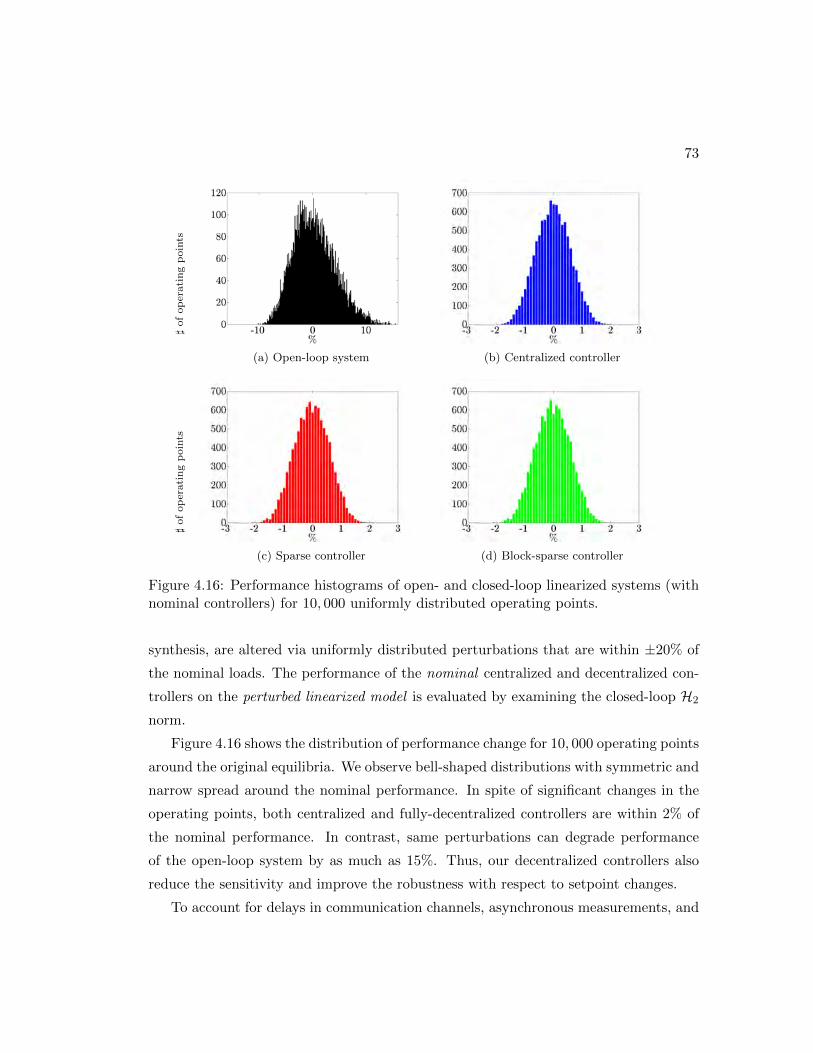
73
]of
op
erati
ng
poin
ts
(a) Open-loop system (b) Centralized controller
]of
op
erati
ng
poin
ts
(c) Sparse controller (d) Block-sparse controller
Figure 4.16: Performance histograms of open- and closed-loop linearized systems (withnominal controllers) for 10, 000 uniformly distributed operating points.
synthesis, are altered via uniformly distributed perturbations that are within ±20% of
the nominal loads. The performance of the nominal centralized and decentralized con-
trollers on the perturbed linearized model is evaluated by examining the closed-loop H2
norm.
Figure 4.16 shows the distribution of performance change for 10, 000 operating points
around the original equilibria. We observe bell-shaped distributions with symmetric and
narrow spread around the nominal performance. In spite of significant changes in the
operating points, both centralized and fully-decentralized controllers are within 2% of
the nominal performance. In contrast, same perturbations can degrade performance
of the open-loop system by as much as 15%. Thus, our decentralized controllers also
reduce the sensitivity and improve the robustness with respect to setpoint changes.
To account for delays in communication channels, asynchronous measurements, and

74
deg
ree
(a) element-wise sparse controller
deg
ree
(b) block-sparse controller
Figure 4.17: Multivariable phase margins as a function of γ.
fast unmodeled dynamics, we utilize multivariable phase margin to quantify the ro-
bustness of our sparse optimal controllers. In Fig. 4.17, we investigate how the phase
margins of the closed-loop systems change with the sparsity-promoting parameter γ.
As our emphasis on sparsity increases, multivariable phase margins degrade gracefully
and stay close to a desirable phase margin of 60◦.
Our approach thus provides a systematic way for designing optimal sparse con-
trollers with favorable robustness margins and performance guarantees even in a fully-
decentralized case.
4.5 Concluding remarks
We have analyzed inter-area oscillations in power systems by studying their power spec-
tral densities and output covariances. Our analysis of the open-loop system identifies
poorly-damped modes that cause inter-area oscillations. We have also designed sparse
and block-sparse feedback controllers that use relative angle measurements to achieve

75
a balance between system performance and controller architecture. By placing increas-
ing weight on the sparsity-promoting term we obtain fully-decentralized feedback gains.
Performance comparisons of open- and closed-loop systems allowed us to understand the
effect of the control design approach both in terms of system performance and with re-
gards to the resulting control architecture. For the IEEE 39 New England model we have
successfully tested our analysis and control design algorithms. We have also provided
a systematic method for optimal retuning of fully-decentralized excitation controllers
that achieves comparable performance to the optimal centralized controller.

Part III
Optimal control in distributed
networks
76

Chapter 5
Design of distributed integral
control action in power networks
Recently distributed integral controllers relying on averaging and communication have
been proposed as effective means for optimal frequency regulation in power systems, load
balancing of network flows, and as natural extensions to static consensus controllers.
Typically, only the questions of stability, disturbance rejection, and steady-state re-
source allocation are addressed in the literature, and the problems of transient perfor-
mance and optimal communication network design remain open. In this chapter we
consider the optimal frequency regulation problem and propose a principled heuristic to
identify the topology and gains of the distributed integral control layer. We employ an
`1-regularized H2-optimal control framework as a means for striking a balance between
network performance and communication requirements [118].
The resulting optimal control problem is solved using the alternating direction
method of multipliers algorithm. For the IEEE 39 New England benchmark problem,
we demonstrate that the identified sparse and distributed integral controller can achieve
reasonable performance relative to the optimal centralized controller. Interestingly, the
identified control architecture is directed and correlates with the generator rotational
inertia and cost coefficients.
77

78
5.1 Synchronous frequency and power sharing
In this section, we briefly summarize background material on synchronous frequency
and economic load sharing. In the linearized swing equations [61]
M ω = − Lp θ − Dω + η + u, (5.1)
(θ, ω) ∈ R2n are the generator rotor angles and frequencies, u ∈ Rn is the governor
control action, and η ∈ Rn is a disturbance input accounting for stochastic fluctuations
in generation and load, which we model as white noise signals. The diagonal matrices
M and D are positive definite with diagonal elements being the generator inertia and
damping coefficients, and Lp = LTp ∈ Rn×n is the network susceptance matrix, We
assume that the network is connected so that Lp1 = O, where 1 and O are vectors of
unit entries and zeros of appropriate sizes.
Synchronous frequency: If one assumes the existence of a synchronous steady-state
with θi = ωsync ∈ R for all i ∈ {1, . . . , n}, then by summing all equations in (5.1) in
steady state, we obtain the synchronous frequency explicitly as
ωsync =
∑ni=1 ui∑ni=1 Di
+
∑ni=1 ηi∑ni=1 Di
. (5.2)
The control objective is to design a secondary control strategy so that the frequency
deviations converge to zero.
Resource allocation: Aside from driving the frequency deviations to zero it is also
desirable to schedule the injections ui(t) to balance load and generation while minimizing
the operational cost [62]:
minimizeu
n∑
i=1
Ei u2i
subject to
n∑
i=1
(ui + ηi) = 0.
(5.3)
Here Ei > 0 is the cost coefficient for source i ∈ {1, . . . , n}. The optimization problem
(5.3) is convex and the essential insight from the optimality conditions is that all units

79
should produce at identical marginal costs of generation:
Ei u∗i = Ej u
∗j for all i, j ∈ {1, . . . , n}. (5.4)
Observe that the budget constraint equation in (5.3) also guarantees a zero frequency
deviation in (5.2). A special case of the identical marginal cost requirement is the
classical proportional power sharing [119] criterion
u∗iPi
=u∗j
Pj, (5.5)
where Pi is the rating of source i. Clearly, the power sharing objective is a special case
of the resource allocation problem (5.3) if one sets each cost coefficient Ei to 1/Pi.
5.2 Distributed integral control
In this section, we first introduce the problem setup and describe a model for frequency
control of power systems. We then formulate the design of distributed integral action as
a static output-feedback control problem. In the absence of sparsity constraints, we use
an augmented Lagrangian method to determine optimal centralized integral controller.
5.2.1 Problem setup
The frequency error can in principle be driven to zero via decentralized integral action
of the formu = −K1 s
s = ω,(5.6)
where s denotes the auxiliary integral states, and K1 is a diagonal feedback matrix.
It is well known, however, that such decentralized integral controllers do not achieve
steady-state optimality [67]. Furthermore, they are prone to instabilities that may arise
from biased measurement errors [69].
To remedy these shortcomings, we consider the distributed averaging-based integral

80
controller also used in [66–70]
u = −E−1 z
z = K1 ω − LI z.(5.7)
Here, z is the vector of auxiliary distributed integral states, E and K1 are diag-
onal matrices of cost coefficients and positive gains, respectively, LI is the Lapla-
cian matrix of a connected communication graph in the integral controller. Since∑n
i=1 zi =∑n
i=1 K1,i ωi, any steady-state solution of (5.7) satisfies ωi = 0, i.e., the
frequency deviations are driven to zero. Because of LIz = −LIEu = 0, any steady-
state solution of (5.7) also satisfies the identical marginal cost criterion (5.4). Hence,
the controller (5.7) achieves optimal frequency regulation.
By substituting (5.7) to (5.1) yields the closed-loop system
θ = ω
M ω = −Lp θ − Dω − E−1 z + η
z = K1 ω − LI z.
(5.8)
Without loss of generality, we assume that integral controllers are installed on all the
generators. We also assume that K1 is a known diagonal matrix and confine our at-
tention to the design of the Laplacian matrix LI . Equivalently, (5.8) can be written
as
θ
ω
z
=
0 I 0
−M−1Lp −M−1D −(EM)−1
0 K1 −K2LI
︸ ︷︷ ︸Acl
θ
ω
z
︸ ︷︷ ︸x
+
0
M−1
0
︸ ︷︷ ︸B1
d
where the control action is embedded in the closed-loop system matrix Acl. Our objec-
tive is to identify topology of LI and to design the corresponding edge weights in order
to optimally enhance performance of the closed-loop network (5.8) in the presence of
stochastic disturbances η.

81
5.2.2 Static output-feedback control problem
The design of LI can be formulated as a static output-feedback problem for a system
with a state-space model
˙x = A x + B1 η + B2 v , (5.9)
where x =[θT ωT zT
]Tis the state vector, and the auxiliary control is defined as
v = −GC2x. Here, G := LI is the control gain to be designed, and the matrices in (5.9)
are partitioned conformably with the state x
A =
0 I 0
−M−1Lp −M−1D −(EM)−1
0 K1 0
B1 =
0
M−1
0
, B2 =
0
0
I
, C2 =
[0 0 I
].
(5.10)
That fact that C2 only contains zero and identity submatrices, enables us to apply
the sparsity-promoting optimal control framework developed in [19–21]. We will discuss
the details later in Section 5.3.
Since the graph Laplacian of the integral controller satisfies LI1 = 0, we can use
similar coordinate transformation on the auxiliary integral states z. It is noteworthy
that the average mode z is not eliminated from the dynamics, because we can see that
absolute value of z is needed to form the integral control action in (5.7), i.e. −E−1 does
not have Laplacian property. Before introducing the coordinate transformation, we first
define the performance output and weight matrices for states and control inputs.
The closed-loop system resulting from (5.9) is given by,
˙x = (A − B2GC2) x + B1 η
y =
[Q1/2
−R1/2GC2
]x.
(5.11)
Here, y is the performance output, R = RT � 0 is the control weight, and the state

82
weight Q = QT � 0 is selected as
Q =
Qθ 0 0
0 Qω 0
0 0 Qz
with Qθ = Qz = I − (1/n)11T and Qω = M . The performance output y in (5.11)
accounts for deviations from the averages of θ and z, as well as the kinetic energy and
the control effort of the system. The choice of performance indices is inspired by [16] for
designing wide-area controller. Hence, ‖y‖22 = xTQx penalizes frequency deviations and
non-identical integral states similar to the distributed averaging-based integral controller
(5.7) thereby accelerating the convergence of the integral error state. Together with
the frequency penalty Qω, the penalty Qθ on non-identical angle variables aids in the
convergence of the dynamics (5.1) as in [15, 16]. Finally, inspired by the quadratic
criterion (5.3) a suitable choice for the control weight is R = E.
In a power system without a slack bus, the generator rotor angles are only defined in
a relative frame of reference, as can be observed in the linearized swing equations (5.1).
Thus, all rotor angles θ can be rotated by a uniform amount without changing the
dynamics (5.1). Since only differences between the components of θ(t) ∈ Rn enter
into (5.8), this rotational symmetry is preserved in the closed-loop system (5.10) as
well.
By introducing a coordinate transformation [16,30]
θ = U ψ + 1 θ, (5.12a)
we can eliminate the marginally stable average mode θ = 1T θ/n from (5.8) and the pre-
serve rotational symmetry. Here, ψ ∈ Rn−1 and the columns of the matrix U ∈ Rn×(n−1)
form an orthonormal basis of the subspace orthogonal to span (1). For example, the
columns of U can be obtained from the (n − 1) eigenvectors of the projector matrix(I − (1/n)11T
). The matrix U has the following properties
UT U = I, U UT = I − (1/n)11T , UT 1 = O.

83
Furthermore, since the Laplacian matrix of the integral controller satisfies LI1 = O, we
can use similar coordinate transformation on the auxiliary integral states z to ensure
the Laplacian property of LI in our control design,
z = U φ + 1 z, (5.12b)
where z = 1T z/n is the average integral state. Note that, in contrast to θ, the average
of the integral state z actually enters into the closed-loop dynamics (5.8).
The structural constraints on θ and z are enforced by the following conditions
Qθ 1 = O, Lp 1 = O
Qz 1 = O, LI 1 = O.
As an additional benefit, the above choice of Qz penalizes the z variable relative to the
vector 1, and thus facilitates the achievement of the identical marginal cost criterion
(5.4).
To eliminate the marginally stable average-angle-mode θ and preserve the relative
information exchange requirement for the dynamics of z, we combine (5.12a) and (5.12b)
to obtain the following coordinate transformation
θ
ω
z
︸ ︷︷ ︸x
=
U 0 0 0
0 I 0 0
0 0 1 U
︸ ︷︷ ︸T1
ψ
ω
z
φ
︸ ︷︷ ︸x
+
1
0
0
0
θ.
(5.13)
Equivalently, x can be expressed in terms of x as
ψ
ω
z
φ
︸ ︷︷ ︸x
=
UT 0 0
0 I 0
0 0 (1/n)1T
0 0 UT
︸ ︷︷ ︸T2
θ
ω
z
︸ ︷︷ ︸x
.(5.14)

84
The properties of the matrix U imply that the matrices T1 and T2 satisfy T2 T1 = I and
T1 T2 =
I − (1/n)11T 0 0
0 I 0
0 0 I
.
In the new set of coordinates, the closed-loop system (5.7) takes the form
x = (A − B2 F C2)x + B1 η
y =
[Q1/2
−R1/2 F C2
]x
(5.15)
where
A = T2 A T1, B1 = T2 B1, Q = T T1 Q T1,
and BT2 =
[0 0 0 U
]T, C2 =
[0 0 0 I
]. The matrices B2 and C2 are parti-
tioned conformably with the partition of the state vector x. The feedback matrices G
and F (in the x and x coordinates, respectively) are related by
F = GU ⇔ G = F UT .
For this static-output feedback problem (5.15), the control objective is to achieve a
desirable tradeoff between the H2 performance of (5.15) and the sparsity of the feedback
gain G. The H2 norm from the disturbance η to the output y, which quantifies the
steady-state variance (energy) of y of the stochastically forced system (5.15), is defined
as
J(F ) :=
trace(BT
1 P (F )B1
)F stabilizing
∞ otherwise
where the closed-loop observability Gramian P satisfies the Lyapunov equation
(A − B2 F C2)TP + P (A − B2 F C2) = − (Q + CT2 FTRF C2).
While the performance is expressed in terms of the feedback gain matrix F , we will

85
enhance sparsity of the Laplacian matrix G = LI in the original coordinates; see Sec-
tion 5.3.
5.2.3 Optimal design of the centralized integral action
We first focus on the design the centralized integral controller G = LI that minimizes the
H2 norm of the closed-loop system, we follow the augmented Lagrangian approach for
structured feedback synthesis [120,121]. Since the matrix C2 in (5.15) only contains zero
and identity submatrices, we can formulate the static output-feedback problem (5.15)
as a structured state-feedback optimal control problem
x = (A − B2K)x + B1 η
y =
[Q1/2
−R1/2K
]x
(5.16)
where K satisfies the following structural constraint
K :=[Kψ Kω Kz Kφ
]=[
0 0 0 F]. (5.17)
Finding a solution of the structured optimal control problem (5.16) amounts to solving
minimizeK
J(K)
subject to K ∈ S,(5.18)
where J(K) is the H2 norm of system (5.16) parameterized as a function of K, and Sis a set of stabilizing feedback gains K satisfying the structural constraint (5.17). The
algebraic characterization of the structural constraint is given by
K ∈ S ⇔ K ◦ IS = K,
where ◦ is the elementwise matrix multiplication and
IS =[
0 0 0 11T]
is partitioned conformably with the partition of the state x.

86
The augmented Lagrangian method developed in [120] solves a sequence of un-
structured problems iteratively, and the minimizers of the unstructured problems con-
verge to a minimizer of the optimal control problem (5.18). The resulting centralized
LI = G = FUT can be used as a warm-start for the sparsity-promoting optimal control
problem that is discussed next.
5.3 Sparsity-promoting optimal control
A sparsity-promoting optimal control framework for finding a state feedback that simul-
taneously optimizes the closed-loop variance and induces a sparse control architecture
was developed in [19–21]. In this section, we extend this approach to a static output-
feedback optimal control problem.
While we want to minimize the H2 norm in terms of the feedback matrix F in
the new set of coordinates, we would like to promote sparsity of the Laplacian matrix
G = LI in the physical domain. This procedure is used to identify sparse structure of
the integral control layer. This is accomplished by considering the regularized optimal
control problem
minimizeF,G
J(F ) + γ g(G)
subject to F UT − G = 0.(SP)
The regularization term in (SP) is determined by
g(G) :=∑
i, j
Wij |Gij |
which is an effective proxy for inducing elementwise sparsity in the feedback gain G [99].
The weights Wij ’s are updated iteratively using the solution to (SP) from the previ-
ous iteration; see [99] for details. In (SP), γ is positive regularization parameter that
characterizes the emphasis on the sparsity level of the feedback matrix G.
The linear constraint in (SP) allows us to exploit structure of the objective func-
tions J and g with the ADMM algorithm. ADMM brings two benefits to the sparsity-
promoting control problem: separability of g(G) and differentiability of J(F ). The
penalty function g(G) is separable with respect to the individual elements of the ma-
trix, however, the closed-loop H2 norm can not be decomposed into componentwise

87
functions of the feedback gain. By separating g(G) and J(F ) in the minimization of the
augmented Lagrangian Lρ, we can determine analytically the solution to the G mini-
mization problem. On the other hand, the square of the closed-loop H2 norm J(F ) is a
differentiable function of F , and this is in contrast to g(G) which is a non-differentiable
function.
Next we describe the ADMM algorithm for solving (SP), see [21, 30] for additional
details.
Initialization
We follow the augmented Lagrangian approach introduced in Section 5.2.3 to design
an optimal F0 = GU to initialize the iterative procedure.
Form augmented Lagrangian
Lρ(F,G,Λ) = J(F ) + γ g(G) + trace(ΛT (F UT − G)
)+
ρ
2‖F UT −G ‖2F
where Λ denotes the matrix of Lagrange multipliers and ‖ · ‖F is the Frobenius norm of
a matrix.
Iterative ADMM algorithm
Fm+1 = argminF
Lρ (F, Gm, Λm)
Gm+1 = argminG
Lρ (Fm+1, G, Λm)
Λm+1 = Λm + ρ (Fm+1 UT − Gm+1).
Here, m represents the iteration index. Using the fact that UTU = I, it is readily shown
that the F -minimization step amounts to solving the following optimization problem
Fm+1 = argminF
(J(F ) +
ρ
2‖F − Hm‖2F
)
where Hm := (Gm − (1/ρ)Λm)U. We apply the KKT necessary conditions [122] for

88
optimality of Lρ(F,Gm,Λm), and the following equations need to be satisfied
(A − B2 F C2)L + L (A − B2 F C2)T = −B1BT1
(A − B2 F C2)TP + P (A − B2 F C2) =
− (Q + CT2 FTRF C2) 2 (RF C2 − BT
2 P )LCT2 + ρ (F − Hm) = 0.
The resulting set of the matrix-valued equations is solved using the iterative procedure
developed in [21].
Similarly, properties of the matrix U can be used to bring the G-minimization prob-
lem into the following form
Gm+1 = argminG
(γ g(G) +
ρ
2‖G − V m‖2F
)
where V m := Fm+1UT + (1/ρ)Λm and the unique solution is obtained via the soft
thresholding operator,
G,+1ij =
(1 − a/|V mij |)V m
ij |V mij | > a
0 |V mij | ≤ a.
Here, a := (γ/ρ)Wij and, for a given V mij , Gm+1
ij is either set to zero or it is obtained by
moving V mij towards zero with the amount (γ/ρ)Wij .
Stopping criterion
‖Fm+1 UT −Gm+1‖ ≤ ε, ‖Gm+1 −Gm‖ ≤ ε
The ADMM algorithm stops when both primal and dual residuals are smaller than
specified thresholds.
Polishing step Finally, we fix the sparsity pattern of G identified using ADMM and
solve the optimal control problem with the identified structural constraints. This pol-
ishing step improves the H2 performance relative to the feedback gain identified by
ADMM; see [21] for additional details.

89
5.4 Case study: IEEE 39 New England model
The IEEE 39 New England Power Grid model consists of 39 buses and 10 detailed
two-axis generator models; see Fig. 5.1. All loads are modeled as constant power loads.
As previously mentioned, we assume that all the generators are equipped with integral
controllers. We extract network susceptance matrix Lp and inertia matrix M of the
IEEE 39 New England model from Power System Toolbox [123]. We set the the damping
coefficients Di of each generator to be 0.1Mi, and the diagonal positive control gain
matrix K1 to be identity matrix. The values of the cost coefficients Ei are chosen to
be Ei = 0.9 for i ∈ {1, 2, 3, 4, 6, 7, 8, 9, 10}, E5 = 0.1, i.e., we assume that generator 5
cost the least to operate while all other generators have the same cost coefficients. The
state matrices and performance indices are defined as outlined in Section 5.2.2.
Next, we illustrate that our proposed static output feedback sparsity-promoting
optimal control framework is an efficient way to achieve a balance between the system
performance and sparsity level of LI . In Fig 5.2, we show the sparsity pattern of the
feedback matrix G = LI ∈ R10×10 for different value of γ. The blue dots denote
local feedback control gains, and the red dots identify information that needs to be
communicated between different generators. For γ = 0.001, LI is dense and recovers
the communication pattern of the conventional integral controller as shown in Fig. 5.2a.
When γ increases from 0.001 to 0.101, the 5th column of LI becomes sparse while the
5th row becomes the only row with all nonzero elements. This indicates that most
generators do not care about generator 5 that has the smallest cost coefficient. At the
same time, integral controller on generator 5 has to gather information from all other
generators to achieve desired performance of the network.
By further increasing γ to 4.715, the structure of LI shows that integral state in-
formation of generator 1, 3, 6, 9, 10, which have the five largest inertia, is gathered by
other integral controllers. Apparently, six other generators need to access information
from generator 10, since it has the largest inertia and thus the most reliable frequency
measurement in the integral control. Finally, when γ = 10, only 11 long-range links are
required, and integral controller on generator 10 is no longer needed. Since generator 10
is an equivalent aggregated model representing the transmission network of a neighbor-
ing area, it has an oversized inertia coefficient and thus also little control agility. Hence,

90
15
512
1110
7
8
9
4
3
1
2
17
18
14
16
19
20
21
24
26
27
28
31
32
34 33
36
38
39 22
35
6
13
30
37
25
29
23
1
10
8
2
3
6
9
4
7
5
F
Fig. 9. The New England test system [10], [11]. The system includes10 synchronous generators and 39 buses. Most of the buses have constantactive and reactive power loads. Coupled swing dynamics of 10 generatorsare studied in the case that a line-to-ground fault occurs at point F near bus16.
test system can be represented by
δi = ωi,Hi
πfsωi = −Diωi + Pmi − GiiE
2i −
10∑
j=1,j =i
EiEj ·
· {Gij cos(δi − δj) + Bij sin(δi − δj)},
⎫⎪⎪⎬⎪⎪⎭
(11)
where i = 2, . . . , 10. δi is the rotor angle of generator i withrespect to bus 1, and ωi the rotor speed deviation of generatori relative to system angular frequency (2πfs = 2π × 60Hz).δ1 is constant for the above assumption. The parametersfs, Hi, Pmi, Di, Ei, Gii, Gij , and Bij are in per unitsystem except for Hi and Di in second, and for fs in Helz.The mechanical input power Pmi to generator i and themagnitude Ei of internal voltage in generator i are assumedto be constant for transient stability studies [1], [2]. Hi isthe inertia constant of generator i, Di its damping coefficient,and they are constant. Gii is the internal conductance, andGij + jBij the transfer impedance between generators iand j; They are the parameters which change with networktopology changes. Note that electrical loads in the test systemare modeled as passive impedance [11].
B. Numerical Experiment
Coupled swing dynamics of 10 generators in thetest system are simulated. Ei and the initial condition(δi(0),ωi(0) = 0) for generator i are fixed through powerflow calculation. Hi is fixed at the original values in [11].Pmi and constant power loads are assumed to be 50% at theirratings [22]. The damping Di is 0.005 s for all generators.Gii, Gij , and Bij are also based on the original line datain [11] and the power flow calculation. It is assumed thatthe test system is in a steady operating condition at t = 0 s,that a line-to-ground fault occurs at point F near bus 16 att = 1 s−20/(60Hz), and that line 16–17 trips at t = 1 s. Thefault duration is 20 cycles of a 60-Hz sine wave. The faultis simulated by adding a small impedance (10−7j) betweenbus 16 and ground. Fig. 10 shows coupled swings of rotorangle δi in the test system. The figure indicates that all rotorangles start to grow coherently at about 8 s. The coherentgrowing is global instability.
C. Remarks
It was confirmed that the system (11) in the New Eng-land test system shows global instability. A few comments
0 2 4 6 8 10-5
0
5
10
15
δi /
rad
10
02
03
04
05
0 2 4 6 8 10-5
0
5
10
15
δi /
rad
TIME / s
06
07
08
09
Fig. 10. Coupled swing of phase angle δi in New England test system.The fault duration is 20 cycles of a 60-Hz sine wave. The result is obtainedby numerical integration of eqs. (11).
are provided to discuss whether the instability in Fig. 10occurs in the corresponding real power system. First, theclassical model with constant voltage behind impedance isused for first swing criterion of transient stability [1]. This isbecause second and multi swings may be affected by voltagefluctuations, damping effects, controllers such as AVR, PSS,and governor. Second, the fault durations, which we fixed at20 cycles, are normally less than 10 cycles. Last, the loadcondition used above is different from the original one in[11]. We cannot hence argue that global instability occurs inthe real system. Analysis, however, does show a possibilityof global instability in real power systems.
IV. TOWARDS A CONTROL FOR GLOBAL SWING
INSTABILITY
Global instability is related to the undesirable phenomenonthat should be avoided by control. We introduce a keymechanism for the control problem and discuss controlstrategies for preventing or avoiding the instability.
A. Internal Resonance as Another Mechanism
Inspired by [12], we here describe the global instabilitywith dynamical systems theory close to internal resonance[23], [24]. Consider collective dynamics in the system (5).For the system (5) with small parameters pm and b, the set{(δ,ω) ∈ S1 × R | ω = 0} of states in the phase plane iscalled resonant surface [23], and its neighborhood resonantband. The phase plane is decomposed into the two parts:resonant band and high-energy zone outside of it. Here theinitial conditions of local and mode disturbances in Sec. IIindeed exist inside the resonant band. The collective motionbefore the onset of coherent growing is trapped near theresonant band. On the other hand, after the coherent growing,it escapes from the resonant band as shown in Figs. 3(b),4(b), 5, and 8(b) and (c). The trapped motion is almostintegrable and is regarded as a captured state in resonance[23]. At a moment, the integrable motion may be interruptedby small kicks that happen during the resonant band. That is,the so-called release from resonance [23] happens, and thecollective motion crosses the homoclinic orbit in Figs. 3(b),4(b), 5, and 8(b) and (c), and hence it goes away fromthe resonant band. It is therefore said that global instability
!"#$%&'''%()(*%(+,-.,*%/012-3*%)0-4%5677*%899: !"#$%&'
(')$
Authorized licensed use limited to: Univ of Calif Santa Barbara. Downloaded on June 10, 2009 at 14:48 from IEEE Xplore. Restrictions apply.
1
10
Figure 5.1: The IEEE 39 New England Power Grid.
(a) γ = 0.001, card (G) = 100 (b) γ = 0.101, card (G) = 91
(c) γ = 4.715, card (G) = 23 (d) γ = 10, card (G) = 20
Figure 5.2: Sparsity pattern of G resulting from (SP).
it is not surprising to drop this virtual controller. Our observation shows that the
optimal communication architecture correlates with both inertia and cost coefficients.
In Fig. 5.3, we compare performance degradation and sparsity level for different

91
(J − Jc) /Jc card (G) /card (Gc)
10−3 10−2 10−1 100 1010
5
10
15
20
γ
perc
ent
10−3 10−2 10−1 100 1010
20
40
60
80
100
γ
perc
ent
Figure 5.3: Performance vs sparsity comparison of sparse G and the optimal centralizedcontroller Gc for 50 logarithmically-spaced points γ ∈ [ 10−3 , 10 ].
values of γ. Compared to the optimal centralized integral controller Gc, our sparse G
in Fig 5.2d degrades system performance by only 16.15%. Therefore, by constructing
only 11 long-range links for the integral controller architecture, reasonable performance
is achieved compared to the optimal centralized feedback gain Gc.
5.5 Concluding remarks
In this section, we propose a distributed PI-control strategy for frequency control in
power systems. We formulate the topology identification and design of integral controller
as a static output-feedback control problem. A coordinate transformation is introduced
to enforce the structural constraints on the rotor angles and auxiliary integral states.
We find the solution by solving the sparsity-promoting optimal control problem, which
balances the tradeoff between system performance and sparsity of the controller. Our
development is validated by a benchmark power system example.

Chapter 6
Design of optimal coupling gains
for synchronization of nonlinear
oscillators
This chapter develops a structured optimal-control framework to design coupling gains
for synchronization of weakly nonlinear oscillator circuits connected in resistive networks
with arbitrary topologies. The oscillators are modeled as weakly nonlinear Lienard-type
circuits, and the coupling gain amounts to the current gain which scales the output
current of the oscillator. The structured optimal-control problem allows us to seek a
decentralized control strategy (equivalently, a diagonal feedback matrix) that precludes
communications between oscillators. To this end, a sparsity-promoting optimal control
algorithm is developed to tune the optimal diagonal feedback-gain matrix with minimal
performance sacrifice [124]. This involves solving an H2 optimal control problem with
`1 regularization by applying the alternating direction method of multipliers (ADMM).
Simulation studies with application to voltage regulation in islanded networks composed
of power-electronic inverters are provided to validate the approach.
92

93
6.1 System of coupled weakly nonlinear oscillator circuits
We begin this section with a description of the oscillator dynamics, and then describe
the network interactions.
6.1.1 Nonlinear oscillator model
The oscillator dynamics are governed by
v + ε f(v) v + ω2v = κ εω u(t) , (6.1)
where v is the terminal voltage, u is the input current, κ is the current gain (interchange-
ably referred as the coupling gain), ε is a positive real constant, and ω is the frequency
of the voltage waveform for the unforced (u = 0) system in the so-called quasi-harmonic
limit ε ↘ 0 [96]. All subsequent discussions assume operation in this quasi-harmonic
limit since the terminal-voltage dynamics in this limit are approximately sinusoidal [96].
Function f : R→ R satisfies the conditions in Lienard’s theorem [84] for existence of a
unique and stable limit cycle, in particular,
(A1) f(v) is continuously differentiable ∀v.
(A2) f(v) is an even function, i.e., f(v) = f(−v),∀v.
(A3) Function F (v) :=∫ v
0 f(z)dz has exactly one positive zero at v = v0, is negative
for 0 < v < v0, is positive and nondecreasing ∀v > v0, and limv→∞
F (v)→∞.
Examples of nonlinear circuits that admit terminal-voltage dynamics of the form (6.1)
include the ubiquitous Van der Pol oscillator (see Fig. 6.1 for more details), the dead-
zone oscillator [85], a class of operational transconductance amplifiers [92], and dynamic
translinear oscillator circuits [91].
To extract the amplitude and phase dynamics from (6.1), we seek a dynamical system
representation in polar coordinates. To this end, define the change of variables v =
r cos(φ), ω∫ t
0 v dt = r sin(φ), where r denotes the radius of the oscillator limit cycle, and
φ represents the instantaneous phase of the resulting oscillations. It is straightforward

94
Figure 6.1: The Van der Pol oscillator circuit with a current gain κ admits the dynamicsin (6.1). In this case, ω = 1/
√LC, ε =
√L/C, and h(v) =
∫f(v)dv = αω(v − βv3/3)
where α and β are positive real constants.
to show that with this change of coordinates, we recover the following model:
r = ε (h(r cosφ) + κω u(t)) cosφ,
φ = ω −(ε
rh(r cosφ) − ε κω
u(t)
r
)sinφ, (6.2)
where h(z) :=
∫f(z)dz. In subsequent developments, we will find it useful to work
with the following model:
r = ε (h(r cos(ωt + θ)) + κω u(t)) cos(ωt + θ),
θ = − εr
(h(r cos(ω t + θ)) + κω u(t)) sin(ω t + θ). (6.3)
where we define θ(t) := φ(t) − ωt, with θ representing the phase offset with respect to
the rotating reference frame of frequency ω. Since the system (6.3) is non-autonomous
but periodic in t, we leverage averaging methods to obtain an autonomous system which
admits similar dynamics [96]. In particular, for small values of ε we can average the
periodic vector fields in (6.3) to obtain the so-called slow flow equations which are
accurate up to O(ε) [125].
Let us denote r and θ to be the 2π/ω-averaged values of the periodic signals r and
θ, respectively. In the quasi-harmonic limit, i.e., ε ↘ 0, we apply standard averaging
arguments using ε as the small parameter, to obtain the averaged dynamics [96, Theorem

95
10.4] [83, 126]
[r
θ
]=εω
2π
∫ 2π/ω
0
[h(r cos(ωt+ θ))) cos(ωt+ θ)
−1rh(r cos(ωt+ θ)) sin(ωt+ θ)
]dt
+εκω2
2π
∫ 2π/ω
0
[u(t) cos(ωt+ θ)
−1ru(t) sin(ωt+ θ)
]dt
=ε
2π
−f(r) + ω2
∫ 2πω
0 u(t) cos(ωt+ θ)dt
−κω2∫ 2π
ω0
u(t)r sin(ωt+ θ)dt
, (6.4)
where
f(r) := 4
∫ r
0f(σ)
√1− σ2
r2 dσ. (6.5)
6.1.2 Resistive electrical network
We consider a collection of N oscillators with dynamics of the form (6.1) (or equiva-
lently, (6.4)) connected in a resistive electrical network. The oscillators are assumed
to be identical in all aspects except for the current gains. The nodes of the resistive
electrical network are collected in the set A, and branches (edges) are collected in the
set E := {(j, `)} ⊂ A × A. Let N := {1, . . . , N} ⊆ A denote nodes that the oscillators
are connected to, and denote the set of internal nodes as I := A\N . Shunt loads—also
modeled as resistances—are connected to the internal nodes I. Denote the vectors that
collect the nodal current injections and node voltages in the network by iA and vA, re-
spectively. Note that since the network is resistive, iA and vA are real-valued functions
of time. The electrical coupling between the oscillators is described by Kirchhoff’s and
Ohm’s laws, which read in matrix-vector form as
iA = GA vA, (6.6)
with entries of the conductance matrix GA given by
[GA]j` :=
gj +∑
(j,k)∈E gjk, if j = `,
−gj`, if (j, `) ∈ E ,0, otherwise,
(6.7)

96
with gj ∈ R≥0 denoting the shunt conductance at node j, and gj` = g`j ∈ R≥0 the
conductance of the line (j, `).
Let i=[i1, . . . , iN ]T and v=[v1, . . . , vN ]T be the vectors of inverter current injections
and terminal voltages, respectively, and let iI and vI be the vectors collecting the current
injections and nodal voltages for the interior nodes. Note that entries of iI are zero.
With this notation in place, we can rewrite (6.6) as
[i
0
]=
[GNN GNI
GTNI GII
][v
vI
]. (6.8)
For the resistive networks we consider in this work, GII is always nonsingular due to
irreducible diagonal dominance [127]. Therefore, the second set of equations in (6.8) can
be uniquely solved for the interior voltages, vI . Then, we obtain the following equations
relating the oscillator current injections and terminal voltages:
i = l(GNN − GNI G
−1II G
TNI)v =: Gv. (6.9)
We refer to the matrix G in (6.9) as the Kron-reduced conductance matrix and this model
reduction through a Schur complement of the conductance matrix is known as Kron
reduction [127]. Notice that the entries of G define the effective electrical conductances
between the oscillators in the network, as well as the effective local resistive loads for
each oscillator. An illustration of Kron reduction for a network with three oscillators is
shown in Fig. 6.2. Under some mild assumptions on the originating network, it follows
that the Kron-reduced network is fully connected [127].
With a slight abuse of notation, we denote the effective shunt-conductance load for
the jth oscillator by gj , and the effective conductance of the (j, `) line in the Kron-
reduced electrical network by gj` in all subsequent discussions. Also, we will find it
useful to define gjj := gj +∑N
k=1,k 6=j gjk.

97
6.1.3 System dynamical model in polar coordinates
With this notation in place, for the resistive network, the current input for the jth
oscillator, uj(t) is given by:
uj(t) = − ij(t) = −N∑
`=1
gj` r` cos(ωt + θ`). (6.10)
Substituting (6.10) in (6.4), and denoting θj` = θj − θ`, we get the following polar-
coordinates representation for the dynamics of the jth oscillator:
drjdt
= −ε f(rj)
2π− κj εω
2gjj rj +
κjεω
2
N∑
`=1,`6=jgj` r` cos(θj`), (6.11a)
dθjdt
= l − κj ε ω
2 rj
N∑
`=1,`6=jgj` r` sin(θj`). (6.11b)
6.1.4 State-space representation of linearized system
Our objective is to design an optimal set of coupling gains, κ1, . . . , κN , that ensure
the terminal voltages of the nonlinear oscillator dynamics in (6.11) are regulated to a
common value. For the class of oscillator models we consider, it is known that there
exists a unique and stable limit cycle with radius req which satisfies f(req) = 0 [84].
With a view towards leveraging control design techniques from linear systems theory,
we linearize the system around (req1N , θeq) (where 1N denotes N ×1 vector of all ones);
Figure 6.2: Kron reduction illustrated for a network of three oscillators. In this example,A = {1, . . . , 5}, N = {1, 2, 3}, and I = {4, 5}.

98
θeq is the phase-synchronized equilibrium (we comment on it next). The Jacobian of
the system around the equilibrium point can be partitioned into blocks as follows:
J =
[JA JB
JC JD
]. (6.12)
The entries of JA, JB, JC, and JD are specified as:
[JA
]j`
=
− ε
2πf ′(req) − κj
εω
2gjj if j = `
κjεω
2gjl cos(θeq,j`) if j 6= `
[JB
]j`
= −κjεω
2gj` req sin(θeq,j`)
[JC
]j`
=
κjε ω
2 req
∑N`=1,`6=j gj` sin(θeq,j`) if j = `
−κjε ω
2gj` sin(θeq,j`) if j 6= `
[JD
]j`
=
0 if j = `
κjε ω
2gj` cos(θeq,j`) if j 6= `
,
where f ′(req) represents the derivative of f(·) evaluated at req. An inspection of the
above Jacobian reveals that the phase-synchronized equilibrium i.e., θeq,j = θeq,` ∀j, `,is locally exponentially stable. First, notice that J is block diagonal for this equilibrium
and therefore around this equilibrium, the evolution of amplitudes and phases are de-
coupled. Furthermore, while JD is a real skew-symmetric matrix (which implies that all
its eigenvalues are purely imaginary), leveraging LaSalle’s invariance principle it can be
shown that phase synchronized equilibrium is locally exponentially stable [128, Theorem
4.3]. With these arguments in place, we proceed with the linearized (and decoupled)
amplitude dynamics.
For small perturbations about the equilibrium point, we express r = 1Nreq+r, where
r := [r1 r2 · · · rN ]T. By defining states x = r, the linearized system can be written in

99
the state-space model
x = lA x + u + B d
= −( ε
2πf′(req)IN +
εω
2KdG
)x + B d (6.13)
where IN is the N ×N identity; A = − ε2π f
′(req)IN ; the control input, u = − εω
2 KdGx
(with a slight abuse of notation with regard to (6.1)); and B is the input matrix for
external disturbances d. Recall that G is the Kron-reduced conductance matrix, and
Kd = diag{κ1, . . . , κN}. With regard to control synthesis, Kd takes the connotation
of the feedback-gain matrix. In general, B can be chosen according to the application;
and in this particular case, we make the choice B = G. With due regard to the optimal
control problem to be formulated in Section 6.2, we define the vector of performance
outputs, z, as follows:
z =
[Q1/2
−R1/2KdG
]x, (6.14)
where Q is the state penalty matrix; and R is the control input penalty matrix.
A cursory inspection of (6.13)-(6.14) indicates two impediments in applying con-
ventional linear feedback control design approaches: i) the closed-loop system is not in
standard feedback control form, (the standard form would be x = (A − GK)x + Bd);
ii) there is a structural constraint on the feedback gain matrix, K, being diagonal (of
the form Kd). To reformulate the problem so that conventional linear feedback control
design approaches can be used, we first introduce a change of variables, ψ = Gx. Note
that G is invertible when the network has shunt loads [129]. The state-space model for
the system in these new coordinates can be expressed in the following form:
ψ = (A − GKd)ψ + B d
ξ =
[Q1/2
−R1/2Kd
]ψ,
(6.15)
whereA = GAG−1, B = GB
Q = G−1 QG−1, R = R.

100
Next, we introduce an optimal control design method that will allow us to synthesize a
diagonal feedback gain matrix.
6.2 Design of current gains
In this section, we introduce a sparsity-promoting optimal control algorithm developed
in [21, 30] to synthesize optimal current gains for the oscillators with the objective of
regulating their terminal voltages to a common value.
6.2.1 Linear quadratic control design
We cast the task of synthesizing the current gains as an optimal feedback control design
problem. With reference to (6.15), we select the state penalty matrix Q = IN to ensure
that the terminal-voltage amplitudes of all circuits coincide. Furthermore, we set the
control input penalty matrix R = ρIN , ρ ∈ R+. The closed-loop H2 norm from input
disturbance d to performance output z is defined as
J(K) :=
trace(BT P (K)B
)K stabilizing
∞ otherwise,(6.16)
where the closed-loop observability Gramian P (K) satisfies the Lyapunov equation
(A − GK)TP + P (A − GK) = −(Q + KTRK), (6.17)
and K is the feedback-gain matrix. Conventional H2 control design methods, such as
the Linear Quadratic Regulator (LQR) problem, provide us with an optimal centralized
controller. In our problem setting, dense feedback gain matrices require communica-
tion links to relay information about oscillator currents. However, we want to ensure
that the feedback matrix is diagonal so that each oscillator only requires local current
measurements. Next, we introduce the sparsity-promoting optimal control algorithm to
incorporate the structure constrain on the feedback matrix K to get a fully diagonal
matrix Kd.

101
Figure 6.3: Sparsity-promoting optimal current gain design illustrated for a Kron-reduced network and two oscillators. As the sparsity emphasis γ increases, K becomessparser and we eventually recover a diagonal matrix, Kd, which corresponds to local cur-rent gains. Dotted lines indicate communication links that correspond to dense feedbackgain matrices.
6.2.2 Sparsity-promoting optimal control
Consider the following optimization problem:
minimize J(K) + γ g(F )
subject to K − F = 0,(6.18)
where J(K) is defined in (6.16), g(F ) is the sparsity-promoting penalty function, and
γ is the emphasis on sparsity. When γ is zero, objective function (6.18) only minimizes
J(K), which provides us with the optimal centralized controller. As γ increases, the
emphasis on the sparsity penalty function increases, so we obtain sparser feedback-
gain matrices, at the expense of system performance. See Fig. 6.3 for an illustration.
By decoupling the objective functions J and g and introducing the linear constraint
K−F = 0 in (6.18), the alternating direction method of multipliers (ADMM) algorithm
suggests a solution approach by exploiting the separability of g and differentiability of
J ; see [21,30] for the details of the algorithm. The penalty function g(F ) is determined
by a weighted `1 norm [21]:
g(F ) :=∑
i, j
Wij |Fij |, (6.19)
where Wij = 1/(|Fij |+ε) are positive weights, see [99] for detailed procedure of selecting
Wij ’s.

102
The algorithm consists of the following steps: First, we form the augmented La-
grangian; then we use ADMM for the augmented Lagrangian minimization, which in-
cludes a K-minimization step, an F -minimization step, and a dual-variable update step.
ADMM identifies a specific sparsity pattern and provides a good initial condition for
the structured feedback design. Finally, we implement a polishing step, which involves
solving a structured H2 problem for the fixed controller structure. Readers are referred
to [21,30] for further information.
6.3 Case study
To verify the effectiveness of our algorithm for optimal current-gain design, we test it on
a resistive network with the same topology as the the IEEE 37-bus benchmark network
and a collection of N = 7 Van der Pol oscillators (see Fig. 6.6 for the network topology).
The dynamics of the oscillators can be described using (6.1) with f(v) = αω(1− βv2),
where α and β are positive constants. (See Fig. 6.1 for a detailed circuit schematic). It
follows from (6.11) that the averaged voltage-amplitude dynamics of the jth oscillator
are:
Figure 6.4: Schematic diagram of the electrical network. The topology is adopted fromthe IEEE 37-bus network.

103
Figure 6.5: Evolution of averaged amplitudes and phases with time for the nonlinearsystem in (6.11).
(J − Jc) /Jc card (K) /card (Kc)
10−4 10−3 10−20
0.2
0.4
0.6
0.8
1·10−2
γ
%
10−4 10−3 10−20
20
40
60
80
100
γ
%
Figure 6.6: Performance versus sparsity comparison of sparse K and the optimal cen-tralized controller Kc.
d
dtrj = − ε αω
(−1
2rj +
β
8r3j
)− κj ε ω
2gjj rj +
κj ε ω
2
N∑
`=1,`6=jgj` r` cos(θj`). (6.20)
Linearizing (6.20) around the stable equilibrium point of the decoupled oscillator, req =
2/√β [96], and acknowledging that the phase-synchronized equilibrium is locally expo-
nentially stable, we recover the state-space model of the form (6.13) with A = −εαωIN .
For the simulations that follow, we pick α = 0.90, β = 4, ω = 2π60 rad/s, ε = 0.19;
conductances of the lines in the IEEE-37-bus network are sourced from [130].

104
Fig. 6.5 shows the averaged voltage magnitude and phase trajectories of all seven
oscillators when we apply unit current gains (without control design) to the original
nonlinear coupled system (6.11). It is evident that the terminal-voltage magnitudes do
not synchronize as time evolves but the phases synchronize innately.
6.3.1 Optimal current-gain design
The sparsity-promoting optimal control problem in (6.18) is solved with 30 logarithmically-
spaced points for γ ∈ [10−4, 10−2]. In Fig. 6.6, we can see that as emphasis on spar-
sity increases, the number of nonzero elements in the feedback matrix—returned by
the cardinality function card(.)—reduces. For γ = 10−2, the sparsity-promoting opti-
mal control algorithm returns a diagonal feedback controller, Kd with diagonal entries:
κ1 = 0.0033, κ2 = 0.0047, κ3 = 0.0026, κ4 = 0.0025, κ5 = 0.0047, κ6 = 0.0038,
κ7 = 0.0029. With this fully decentralized controller, we drop 80% of the nonzero ele-
ments in the feedback matrix compared to the optimal centralized controller (denoted
by Kc with corresponding cost Jc), at the expense of only 0.01% performance loss.
(a) Linearized system (b) Nonlinear system
Figure 6.7: Oscillator terminal-voltage magnitudes with designed current gains appliedat time t = 0.1 s.

105
6.3.2 Time-domain simulations for original nonlinear and linearized
models
To demonstrate the efficacy of our control design method, we simulate both the linear
model (6.15) and the original nonlinear model (6.20) for Van der pol oscillators, with
the optimal κ’s that are obtained from the sparsity-promoting optimal control algo-
rithm. Fig. 6.7 shows the trajectories of the averaged terminal-voltage magnitudes for
each inverter with optimal gains applied at time t = 0.1 s, with unit current gains as
initial values. From the figure, it is clear that calibrating the current gains leads to
synchronization of terminal voltage amplitudes. Furthermore, since the original nonlin-
ear system also achieves amplitude synchronization, it validates our linearized design
perspective.
6.4 Concluding remarks
In this chapter, we introduced a systematic way of designing current gains for weakly
nonlinear circuits governed by Lienard’s equation in a resistive electrical network. The
output current of each oscillator is scaled by a current gain; and the objective is to
synthesize an optimal set of current gains to ensure voltage regulation in the network.
We apply a sparsity-promoting optimal control method to design the current gains. The
optimization problem targets simultaneously achieving a desirable system performance
and preserving the sparsity pattern, which is the diagonal structure of the feedback
matrix. An iterative ADMM algorithm is used to solve the `1 regularized version of the
standard H2 optimal control problem. Ongoing research is focused on extending the
approach to cover networks with inductive and capacitive elements.

References
[1] M. Mesbahi and M. Egerstedt. Graph Theoretic Methods in Multiagent Networks.
Princeton University Press, 2010.
[2] L. Xiao, S. Boyd, and S.-J. Kim. Distributed average consensus with least-mean-
square deviation. J. Parallel Distrib. Comput., 67(1):33–46, 2007.
[3] A. Ghosh, S. Boyd, and A. Saberi. Minimizing effective resistance of a graph.
SIAM Review, 50(1):37–66, 2008.
[4] W. Ren. Synchronization of coupled harmonic oscillators with local interaction.
Automatica, 44:3195–3200, 2008.
[5] D. Zelazo and M. Mesbahi. Edge agreement: Graph-theoretic performance bounds
and passivity analysis. IEEE Trans. Automat. Control, 56(3):544–555, 2011.
[6] B. Bamieh, M. R. Jovanovic, P. Mitra, and S. Patterson. Coherence in large-
scale networks: dimension dependent limitations of local feedback. IEEE Trans.
Automat. Control, 57(9):2235–2249, 2012.
[7] F. Dorfler and F. Bullo. Synchronization and transient stability in power networks
and non-uniform Kuramoto oscillators. SIAM Journal on Control and Optimiza-
tion, 50:1616–1642, 2012.
[8] A. Mauroy, P. Sacre, and R. J. Sepulchre. Kick synchronization versus diffusive
synchronization. In Proceedings of the 51st IEEE Conference on Decision and
Control, pages 7171–7183, 2012.
106

107
[9] M. Arcak. Synchronization and pattern formation in diffusively coupled systems.
In Proceedings of the 51st IEEE Conference on Decision and Control, pages 7184–
7192, 2012.
[10] D. Zelazo, S. Schuler, and F. Allgower. Performance and design of cycles in
consensus networks. Syst. Control Lett., 62(1):85–96, 2013.
[11] M. Fardad, F. Lin, and M. R. Jovanovic. Design of optimal sparse interconnection
graphs for synchronization of oscillator networks. IEEE Trans. Automat. Control,
59(9):2457–2462, 2014.
[12] G. E. Dullerud and F. Paganini. A course in robust control theory. Springer, 2000.
[13] M. R. Jovanovic and N. K. Dhingra. Controller architectures: tradeoffs between
performance and structure. Eur. J. Control, 30:76–91, July 2016.
[14] F. Dorfler, M. R. Jovanovic, M. Chertkov, and F. Bullo. Sparse and optimal wide-
area damping control in power networks. In Proceedings of the 2013 American
Control Conference, pages 4295–4300, 2013.
[15] F. Dorfler, M. R. Jovanovic, M. Chertkov, and F. Bullo. Sparsity-promoting opti-
mal wide-area control of power networks. IEEE Trans. Power Syst., 29(5):2281–
2291, 2014.
[16] X. Wu, F. Dorfler, and M. R. Jovanovic. Input-output analysis and decentralized
optimal control of inter-area oscillations in power systems. IEEE Trans. Power
Syst., 31(3):2434–2444, May 2016.
[17] B. Bamieh, F. Paganini, and M. A. Dahleh. Distributed control of spatially in-
variant systems. IEEE Trans. Automat. Control, 47(7):1091–1107, 2002.
[18] M. Rotkowitz and S. Lall. A characterization of convex problems in decentralized
control. IEEE Trans. Automat. Control, 51(2):274–286, 2006.
[19] M. Fardad, F. Lin, and M. R. Jovanovic. Sparsity-promoting optimal control
for a class of distributed systems. In Proceedings of the 2011 American Control
Conference, pages 2050–2055, 2011.

108
[20] F. Lin, M. Fardad, and M. R. Jovanovic. Sparse feedback synthesis via the al-
ternating direction method of multipliers. In Proceedings of the 2012 American
Control Conference, pages 4765–4770, 2012.
[21] F. Lin, M. Fardad, and M. R. Jovanovic. Design of optimal sparse feedback
gains via the alternating direction method of multipliers. IEEE Trans. Automat.
Control, 58(9):2426–2431, 2013.
[22] N. Matni. Communication delay co-design in H2 distributed control using atomic
norm minimization. IEEE Trans. Control Netw. Syst., 2016. accepted; also
arXiv:1404.4911.
[23] N. Matni and V. Chandrasekaran. Regularization for design. IEEE Trans. Au-
tomat. Control, 2016. accepted; also arXiv:1404.1972.
[24] S. Boyd, N. Parikh, E. Chu, B. Peleato, and J. Eckstein. Distributed optimiza-
tion and statistical learning via the alternating direction method of multipliers.
Foundations and Trends in Machine Learning, 3(1):1–124, 2011.
[25] Bassam Bamieh and Petros G Voulgaris. A convex characterization of distributed
control problems in spatially invariant systems with communication constraints.
Systems & Control Letters, 54(6):575–583, 2005.
[26] Michael Rotkowitz and Sanjay Lall. A characterization of convex problems in
decentralized control. IEEE Trans. Automat. Control, 51(2):274–286, Feb 2006.
[27] Anders Rantzer. Distributed control of positive systems. In Proceedings of 50th
IEEE Conference on Decision and Control, pages 6608–6611, Dec 2011.
[28] N. K. Dhingra, M. Colombino, and M. R. Jovanovic. On the convexity of a class
of structured optimal control problems for positive systems. In Proceedings of the
2016 European Control Conference, pages 825–830, 2016.
[29] F. Lin, M. Fardad, and M. R. Jovanovic. Identification of sparse communication
graphs in consensus networks. In Proceedings of the 50th Annual Allerton Confer-
ence on Communication, Control, and Computing, pages 85–89, Monticello, IL,
2012.

109
[30] X. Wu and M. R. Jovanovic. Sparsity-promoting optimal control of consensus and
synchronization networks. In Proceedings of the 2014 American Control Confer-
ence, pages 2948–2953, 2014.
[31] S. Hassan-Moghaddam and M. R. Jovanovic. An interior point method for grow-
ing connected resistive networks. In Proceedings of the 2015 American Control
Conference, pages 1223–1228, Chicago, IL, 2015.
[32] S. Hassan-Moghaddam and M. R. Jovanovic. Topology design for stochastically-
forced consensus networks. IEEE Trans. Control Netw. Syst., 2016. submitted;
also arXiv:1506.03437v3.
[33] B. Polyak, M Khlebnikov, and P. Shcherbakov. An LMI approach to structured
sparse feedback design in linear control systems. In Proceedings of the 2013 Eu-
ropean Control Conference, pages 833–838, 2013.
[34] N. K. Dhingra, M. R. Jovanovic, and Z. Q. Luo. An ADMM algorithm for optimal
sensor and actuator selection. In Proceedings of the 53rd IEEE Conference on
Decision and Control, pages 4039–4044, 2014.
[35] N. K. Dhingra and M. R. Jovanovic. Convex synthesis of symmetric modifications
to linear systems. In Proceedings of the 2015 American Control Conference, pages
3583–3588, 2015.
[36] S. Schuler, P. Li, J. Lam, and F Allgower. Design of structured dynamic output-
feedback controllers for interconnected systems. International Journal of Control,
84(12):2081–2091, 2011.
[37] Nikolai Matni and Venkat Chandrasekaran. Regularization for design. In Pro-
ceedings of the 53rd IEEE Conference on Decision and Control, pages 1111–1118,
Los Angeles, CA, 2014.
[38] D. M. Zoltowski, N. K. Dhingra, F. Lin, and M. R. Jovanovic. Sparsity-promoting
optimal control of spatially-invariant systems. In Proceedings of the 2014 American
Control Conference, pages 1261–1266, 2014.

110
[39] Fernando Alvarado, Chris DeMarco, Ian Dobson, Pete Sauer, Scott Greene, Hen-
rik Engdahl, and Jianfeng Zhang. Avoiding and suppressing oscillations. PSERC
Project Final Report, 1999.
[40] K Prasertwong, N Mithulananthan, and D Thakur. Understanding low-frequency
oscillation in power systems. International Journal of Electrical Engineering Ed-
ucation, 47(3):248–262, 2010.
[41] L Rouco. Eigenvalue-based methods for analysis and control of power system
oscillations. In IEE Colloquium on Power System Dynamics Stabilisation. IET,
1998.
[42] Graham Rogers. Demystifying power system oscillations. IEEE Computer Appli-
cations in Power, 9(3):30–35, 1996.
[43] M. Klein, G. J. Rogers, and P. Kundur. A fundamental study of inter-area oscil-
lations in power systems. IEEE Trans. Power Syst., 6(3):914–921, 1991.
[44] M. Klein, G. J. Rogers, S. Moorty, and P. Kundur. Analytical investigation of
factors influencing power system stabilizers performance. IEEE Transactions on
Energy Conversion, 7(3):382–390, 1992.
[45] N. Martins and L. T. G. Lima. Eigenvalue and frequency domain analysis of
small-signal electromechanical stability problems. In IEEE/PES Symposium on
Applications of Eigenanalysis and Frequency Domain Methods, pages 17–33, 1989.
[46] T. Othman, J. J. Sanchez-Gasca, M. A. Kale, and J. H. Chow. On the design of
robust power system stabilizers. In Proceedings of the 28th IEEE Conference on
Decision and Control, pages 1853–1857, 1989.
[47] O. P. Malik, G. S. Hope, Y. M. Gorski, V. A. Uskakov, and A. L. Rackevich.
Experimental studies on adaptive microprocessor stabilizers for synchronous gen-
erators. IFAC Power System and Power Plant Control, pages 125–130, 2014.
[48] C. Zhu, M. Khammash, V. Vittal, and W. Qiu. Robust power system stabilizer
design using H∞ loop shaping approach. IEEE Trans. Power Syst., 18(2):810–818,
2003.

111
[49] J. A. Taylor and L. Scardovi. Decentralized control of DC-segmented power sys-
tems. In Proceedings of the 52th Annual Allerton Conference, pages 1046–1050,
2014.
[50] J. Xiao, F. Wen, C. Y. Chung, and K. P. Wong. Wide-area protection and its
applications–a bibliographical survey. In IEEE PES Power Systems Conference
and Exposition, pages 1388–1397, 2006.
[51] K. Seethalekshmi, S. N. Singh, and S. C. Srivastava. Wide-area protection and
control: Present status and key challenges. In Fifteenth National Power Systems
Conference, pages 169–175, 2008.
[52] A. Heniche and I. Karnwa. Control loops selection to damp inter-area oscillations
of electrical networks. IEEE Trans. Power Syst., 17(2):378–384, 2002.
[53] L. P. Kunjumuhammed, R. Singh, and B. C. Pal. Robust signal selection for
damping of inter-area oscillations. IET Generation, Transmission & Distribution,
6(5):404–416, 2012.
[54] G. E. Boukarim, S. Wang, J. H. Chow, G. N. Taranto, and N. Martins. A com-
parison of classical, robust, and decentralized control designs for multiple power
system stabilizers. IEEE Trans. Power Syst., 15(4):1287–1292, 2000.
[55] Y. Zhang and A. Bose. Design of wide-area damping controllers for interarea
oscillations. IEEE Trans. Power Syst., 23(3):1136–1143, 2008.
[56] M. Zima, M. Larsson, P. Korba, C. Rehtanz, and G. Andersson. Design aspects for
wide-area monitoring and control systems. Proceedings of the IEEE, 93(5):980–
996, 2005.
[57] S. Schuler, U. Munz, and F. Allgower. Decentralized state feedback control for
interconnected systems with application to power systems. Journal of Process
Control, 24(2):379–388, 2014.
[58] S. Pirooz, J. A. Taylor, and R. Iravani. Decentralized supplementary control of
multiple LCC-HVDC links. IEEE Trans. Power Syst., 2015.
112
[59] J. H. Chow and K. W. Cheung. A toolbox for power system dynamics and control
engineering education and research. IEEE Trans. Power Syst., 7(4):1559–1564,
1992.
[60] B. E. Eliasson and D. J. Hill. Damping structure and sensitivity in the NORDEL
power system. IEEE Trans. Power Syst., 7(1):97–105, 1992.
[61] J. Machowski, J. W. Bialek, and J. R. Bumby. Power System Dynamics. John
Wiley & Sons, 2 edition, 2008.
[62] A. J. Wood and B. F. Wollenberg. Power Generation, Operation, and Control.
John Wiley & Sons, 2 edition, 1996.
[63] Joshua Adam Taylor, Sairaj V Dhople, and Duncan S Callaway. Power systems
without fuel. arXiv preprint arXiv:1506.04799, 2015.
[64] S.T. Cady and A.D. Dominguez-Garcia. Distributed generation control of small-
footprint power systems. In North American Power Symposium (NAPS), 2012.
IEEE, 2012.
[65] Na Li, Lijun Chen, Changhong Zhao, and Steven H Low. Connecting automatic
generation control and economic dispatch from an optimization view. In American
Control Conference, pages 735–740, 2014.
[66] J. W. Simpson-Porco, F. Dorfler, and F. Bullo. Synchronization and power sharing
for droop-controlled inverters in islanded microgrids. Automatica, 49(9):2603–
2611, 2013.
[67] F. Dorfler, J. W. Simpson-Porco, and F. Bullo. Breaking the hierarchy: Dis-
tributed control and economic optimality in microgrids. IEEE Transactions on
Control of Network Systems, 3(3):241–253, 2016.
[68] C. Zhao, E. Mallad, and F. Dorfler. Distributed frequency control for stability
and economic dispatch in power networks. In Proceedings of the 2015 American
Control Conference, pages 2359–2364, Chicago, IL, 2015.

113
[69] M. Andreasson, D. V. Dimarogonas, H. Sandberg, and K. H. Johansson. Dis-
tributed control of networked dynamical systems: Static feedback, integral action
and consensus. IEEE Transactions on Automatic Control, 59(7):1750–1764, 2014.
[70] M. Andreasson, D. V. Dimarogonas, H. Sandberg, and K. H. Johansson. Dis-
tributed PI-control with applications to power systems frequency control. In Pro-
ceedings of the 2014 American Control Conference, pages 3183–3188, 2014.
[71] S. Bennett. Nicholas minorsky and the automatic steering of ships. IEEE Cntrol
Systems Magazine, 4(4):10–15, 1984.
[72] Karl Johan Astrom and Tore Hagglund. The future of PID control. Control
Engineering Practice, 9(11):1163–1175, 2001.
[73] Mathias Burger and Claudio De Persis. Dynamic coupling design for nonlinear
output agreement and time-varying flow control. Automatica, 51:210–222, 2015.
[74] Jieqiang Wei and AJ van der Schaft. Load balancing of dynamical distribution
networks with flow constraints and unknown in/outflows. Systems & Control
Letters, 62(11):1001–1008, 2013.
[75] D. Burbano and M. di Bernardo. Consensus and synchronization of complex
networks via proportional-integral coupling. In Circuits and Systems (ISCAS),
2014 IEEE International Symposium on, pages 1796–1799. IEEE, 2014.
[76] He Bai, Randy Freeman, Kevin M Lynch, et al. Robust dynamic average con-
sensus of time-varying inputs. In Decision and Control (CDC), 2010 49th IEEE
Conference on, pages 3104–3109. IEEE, 2010.
[77] Randy A Freeman, Peng Yang, Kevin M Lynch, et al. Stability and convergence
properties of dynamic average consensus estimators. In IEEE conf. on decision
and control, pages 398–403, 2006.
[78] Andrej Jokic, Mircea Lazar, and PPJ Van den Bosch. Real-time control of power
systems using nodal prices. International Journal of Electrical Power & Energy
Systems, 31(9):522–530, 2009.

114
[79] Lin-Yu Lu. Consensus-based P −f and Q− V droop control for multiple parallel-
connected inverters in lossy networks. In IEEE International Symposium on In-
dustrial Electronics, Taipei, Taiwan, May 2013.
[80] C. Zhao, E. Mallada, and F. Dorfler. Distributed frequency control for stability
and economic dispatch in power networks. In American Control Conference, 2015.
[81] X. Wu, F. Dorfler, and M. R. Jovanovic. Analysis and design trade-offs for power
network inter-area oscillations. In Proceedings of the 21st International Symposium
on Mathematical Theory of Network and Systems, pages 657–663, Groningen, The
Netherlands, 2014.
[82] X. Wu, F. Dorfler, and M. R. Jovanovic. Decentralized optimal control of inter-
area oscillations in bulk power systems. In Proceedings of the 54th IEEE Confer-
ence on Decision and Control, pages 5532–5537, Osaka, Japan, 2015.
[83] S Emre Tuna. Synchronization analysis of coupled lienard-type oscillators by
averaging. Automatica, 48(8):1885–1891, 2012.
[84] Steven H. Strogatz. Nonlinear Dynamics and Chaos: With Applications to
Physics, Biology, Chemistry, and Engineering. Studies in nonlinearity. Westview
Press, 1 edition, Jan. 2001.
[85] B. B. Johnson, S. V. Dhople, A. O. Hamadeh, and P. T. Krein. Synchronization of
parallel single-phase inverters with virtual oscillator control. IEEE Trans. Power
Electron., 29(11):6124–6138, Nov. 2014.
[86] L. A. B. Torres, J. P. Hespanha, and J. Moehlis. Power supplies dynamical
synchronization without communication. In Proceedings of the Power & Energy
Society 2012 General Meeting, July 2012.
[87] Kresimir Josic and Slaven Peles. Synchronization in networks of general,
weakly nonlinear oscillators. Journal of Physics A: Mathematical and General,
37(49):11801, 2004.
[88] Florian Dorfler and Francesco Bullo. Synchronization in complex networks of
phase oscillators: A survey. Automatica, 50(6):1539–1564, 2014.

115
[89] A. Mauroy, P. Sacre, and R. J. Sepulchre. Kick synchronization versus diffusive
synchronization. In IEEE Conference on Decision and Control, pages 7171–7183,
2012.
[90] T. Koga and M. Shinagawa. An extension of the lienard theorem and its appli-
cation [nonlinear circuits]. In Circuits and Systems, 1991., IEEE International
Sympoisum on, pages 1244–1247 vol.2, Jun 1991.
[91] Wouter A Serdijn, Jan Mulder, Albert C van der Woerd, and Arthur HM van
Roermund. A wide-tunable translinear second-order oscillator. Solid-State Cir-
cuits, IEEE Journal of, 33(2):195–201, 1998.
[92] Kofi Odame. Exploiting Device Nonlinearity in Analog Circuit Design. PhD thesis,
Georgia Institute of Technology, 2008.
[93] Pietro De Lellis, Mario di Bernardo, and Franco Garofalo. Synchronization of
complex networks through local adaptive coupling. Chaos: An Interdisciplinary
Journal of Nonlinear Science, 18(3), 2008.
[94] S Emre Tuna. LQR-based coupling gain for synchronization of linear systems.
arXiv preprint arXiv:0801.3390, 2008.
[95] A. Hamadeh, G.-B. Stan, and J. Goncalves. Constructive synchronization of
networked feedback systems. In IEEE Conference on Decision and Control, pages
6710–6715, December 2010.
[96] H. K. Khalil. Nonlinear Systems. Prentice Hall, 3 edition, 2002.
[97] X. Wu and M. R. Jovanovic. Sparsity-promoting optimal control of systems with
symmetries, consensus and synchronization networks. Syst. Control Lett., 2016.
submitted.
[98] Prabha Kundur, Neal J Balu, and Mark G Lauby. Power system stability and
control, volume 7. McGraw-hill New York, 1994.
[99] E. J. Candes, M. B. Wakin, and S. P. Boyd. Enhancing sparsity by reweighted `1
minimization. J. Fourier Anal. Appl, 14:877–905, 2008.

116
[100] M. Yuan and Y. Lin. Model selection and estimation in regression with grouped
variables. Journal of the Royal Statistical Society: Series B (Statistical Method-
ology), 68(1):49–67, 2006.
[101] A. Beck and M. Teboulle. A fast iterative shrinkage-thresholding algorithm for
linear inverse problems. SIAM Journal on Imaging Sciences, 2(1):183–202, 2009.
[102] J. Barzilai and J. M. Borwein. Two-point step size gradient methods. IMA Journal
of Numerical Analysis, 8(1):141–148, 1988.
[103] N. K. Dhingra, X. Wu, and M. R. Jovanovic. Sparsity-promoting optimal control
of systems with invariances and symmetries. In Proceedings of the 10th IFAC
Symposium on Nonlinear Control Systems, pages 648–653, Monterey, CA, 2016.
[104] N. K. Dhingra and M. R. Jovanovic. A method of multipliers algorithm for
sparsity-promoting optimal control. In Proceedings of the 2016 American Control
Conference, pages 1942–1947, Boston, MA, 2016.
[105] N. K. Dhingra and M. R. Jovanovic. The proximal augmented Lagrangian method
for nonsmooth composite optimization. IEEE Trans. Automat. Control, 2016.
submitted; also arXiv:1610.04514.
[106] M. Fardad, F. Lin, and M. R. Jovanovic. On optimal link creation for facilitation
of consensus in social networks. In Proceedings of the 2014 American Control
Conference, pages 3802–3807, Portland, OR, 2014.
[107] V. Jonsson, A. Rantzer, and R. M. Murray. A scalable formulation for engineering
combination therapies for evolutionary dynamics of disease. Proceedings of the
2014 American Control Conference, 2014.
[108] V. Jonsson, N. Matni, and R. M. Murray. Reverse engineering combination ther-
apies for evolutionary dynamics of disease: An H∞ approach. In Proceedings of
the 52nd IEEE Conference on Decision and Control, pages 2060–2065, 2013.
[109] G. E. Dullerud and F. Paganini. A course in robust control theory: a convex
approach, volume 36. Springer Science & Business Media, 2013.

117
[110] J. Swift and P. C. Hohenberg. Hydrodynamic fluctuations at the convective in-
stability. Physical Review A, 15(1):319, 1977.
[111] J. A. C. Weideman and S. C. Reddy. A MATLAB differentiation matrix suite.
ACM Transactions on Mathematical Software, 26(4):465–519, December 2000.
[112] M. Grant and S. Boyd. CVX: Matlab software for disciplined convex programming,
version 2.0 beta. http://cvxr.com/cvx, September 2013.
[113] J. H. Chow and P. Kokotovic. Time scale modeling of sparse dynamic networks.
IEEE Trans. Automat. Control, 30(8):714–722, 1985.
[114] D. Romeres, F. Dorfler, and F. Bullo. Novel results on slow coherency in consensus
and power networks. In Proceedings of the 12th European Control Conference,
pages 742–747, 2013.
[115] L. N. Trefethen and M. Embree. Spectra and pseudospectra: the behavior of non-
normal matrices and operators. Princeton University Press, 2005.
[116] M. R. Jovanovic and B. Bamieh. Componentwise energy amplification in channel
flows. J. Fluid Mech., 534:145–183, 2005.
[117] B. K. Lieu, M. R. Jovanovic, and S. Kumar. Worst-case amplification of distur-
bances in inertialess Couette flow of viscoelastic fluids. J. Fluid Mech., 723:232–
263, May 2013.
[118] X. Wu, F. Dorfler, and M. R. Jovanovic. Topology identification and design of
distributed integral action in power networks. In Proceedings of the 2016 American
Control Conference, pages 5921–5926, Boston, MA, 2016.
[119] J. M Guerrero, M. Chandorkar, T.-L. Lee, and P. C. Loh. Advanced control archi-
tectures for intelligent microgrids, part i: decentralized and hierarchical control.
IEEE Transactions on Industrial Electronics, 60(4):1254–1262, 2013.
[120] F. Lin, M. Fardad, and M. R. Jovanovic. Augmented Lagrangian approach to
design of structured optimal state feedback gains. IEEE Trans. Automat. Control,
56(12):2923–2929, December 2011.

118
[121] M. Fardad, F. Lin, and M. R. Jovanovic. On the optimal design of structured
feedback gains for interconnected systems. In Proceedings of the 48th IEEE Con-
ference on Decision and Control, pages 978–983, Shanghai, China, 2009.
[122] D. P. Bertsekas. Nonlinear programming. Athena Scientific, 1999.
[123] J. H. Chow and K. W. Cheung. A toolbox for power system dynamics and con-
trol engineering education and research. IEEE Transactions on Power Systems,
7(4):1559–1564, 1992.
[124] V. Purba, X. Wu, M. Sinha, S. V. Dhople, and M. R. Jovanovic. Design of optimal
coupling gains for synchronization of nonlinear oscillators. In Proceedings of the
54th IEEE Conference on Decision and Control, pages 1310–1315, Osaka, Japan,
2015.
[125] R. H. Rand. Lecture notes on nonlinear vibrations. 2012.
[126] M. Sinha, F. Dorfler, B. B. Johnson, and S. V. Dhople. Uncovering droop control
laws embedded within the nonlinear dynamics of van der pol oscillators. IEEE
Trans. Control of Networked Sys., 2014. In review.
[127] F. Dorfler and F. Bullo. Kron reduction of graphs with applications to electri-
cal networks. IEEE Transactions on Circuits and Systems I: Regular Papers,
60(1):150–163, Jan. 2013.
[128] F. Dorfler and F. Bullo. Exploring synchronization in complex oscillator networks.
In Proceedings of the 51th IEEE Conference on Decision and Control, pages 7157–
7170, 2012.
[129] S. V. Dhople, B. B. Johnson, F. Dorfler, and A. O. Hamadeh. Synchronization of
nonlinear circuits in dynamic electrical networks with general topologies. Circuits
and Systems I: Regular Papers, IEEE Transactions on, 61(9):2677–2690, 2014.
[130] L. Ling and S. V. Dhople. Spatiotemporal model reduction of inverter-based
islanded microgrids. IEEE Transactions on Energy Conversion, 29(4):823–832,
Dec 2014.


