

ISSN: 2277-9655
[Kamuju* et al., 5(10): October, 2016] Impact Factor: 4.116
IC™ Value: 3.00 CODEN: IJESS7
http: // www.ijesrt.com © International Journal of Engineering Sciences & Research Technology
[676]
IJESRT INTERNATIONAL JOURNAL OF ENGINEERING SCIENCES & RESEARCH
TECHNOLOGY
SPATIAL IDENTIFICATION AND CLASSIFICATION OF SOIL EROSION PRONE
ZONES USING REMOTE SENSING & GIS INTEGRATED ‘RUSLE’ MODEL AND
‘SATEEC GIS SYSTEM’ Narasayya Kamuju*
* Assistant Research Officer, Central Water and Power Research Station, pune, India
DOI: 10.5281/zenodo.163095
ABSTRACT Soil erosion by water is pronounced critical problem in Himalayan regions due to anthropogenic pressure on its
mountainous landscape. Its assessment and mapping of erosion prone areas are very essential for soil conservation
and watershed management. The purpose of this study is to investigate the spatial distribution of average annual
soil erosion in Ton Watershed (a sub-basin of Asan watershed) using Remote Sensing and GIS integrated
‘RUSLE’ Model and GIS based Hydrological Model of ‘SATEEEC GIS system’ in Dehradun district of
Uttarakhand state. Remote sensing and GIS technologies were used to prepare required input layers in the form
of Rain Erosivity factor (R), soil erodability factor( K), Length and steepness of Slope factors (LS), crop
management factors ( C) and support practice factor ( P) to utilize in RUSLE and SATEEC GIS Models. One of
the advantages of using SATEEC GIS system is no additional input data, other than those for RUSLE are required
to operate the system. Vulnerability to soil erosion risk in the watershed revealed that 24.16 percent of area from
RUSLE model, and 20.21 percent of area from SATEEC GIS system was in high soil erosion risk zone. Very low
risk of erosion was observed at 68.18 percent and 57.12 percent of areas from SATEEC GIS system and RUSLE
model respectively.
KEYWORDS: RUSLE, SATEEC GIS System, R-factor, LS-factor, Soil Erosion, ArcGIS.
INTRODUCTION Soil erosion in watershed areas and the subsequent deposition in rivers, lakes and reservoirs are of great concern
for two reasons. Firstly, rich fertile soil is eroded from the watershed areas. Secondly, there is a reduction in
reservoir capacity as well as degradation of downstream water quality [1]. Although sedimentation occurs
naturally, it is exacerbated by poor land use and land management practices adopted in the upland areas of
watersheds. Uncontrolled deforestation due to forest fires, grazing, incorrect methods of tillage and unscientific
agriculture practices are some of the poor land management practices that accelerate soil erosion, resulting in large
increases in sediment inflow into streams [2]. Therefore, prevention of soil erosion is of paramount importance in
the management and conservation of natural resources [3]. The application of RS and GIS techniques makes soil
erosion estimation and its spatial distribution to be determined at reasonable costs and better accuracy in larger
areas. A combination of RS, GIS, and RUSLE is an effective tool to estimate soil loss on a cell-by-cell basis [4].
GIS tools were used for derivation of the topographic factor from DEM data, data interpolation of sample plots,
calculation of soil erosion loss and sediment yield [5]. To estimate soil erosion and to develop optimal soil erosion
management plans, many erosion models, such as Universal Soil Loss Equation (USLE) [6], Water Erosion
Prediction Project (WEPP) [7], Soil and Water Assessment Tool (SWAT) [8], and European Soil Erosion Model
(EUROSEM) [9], have been developed and used over the years. The new version of the USLE model, called the
Revised Universal Soil Loss Equation (RUSLE), a desktop-based model, was developed by modifying the USLE
to more accurately estimate the R, K, C, P factors of soil loss equation, and soil erosion losses [10]. GIS-based
Sediment Assessment Tool for Effective Erosion Control (SATEEC) system was used to estimate soil loss and
sediment yield for any location within a watershed by a combined application of RUSLE and a spatially distributed
sediment delivery ratio within the ArcView GIS software environment [11].
ISSN: 2277-9655
[Kamuju* et al., 5(10): October, 2016] Impact Factor: 4.116
IC™ Value: 3.00 CODEN: IJESS7
http: // www.ijesrt.com © International Journal of Engineering Sciences & Research Technology
[677]
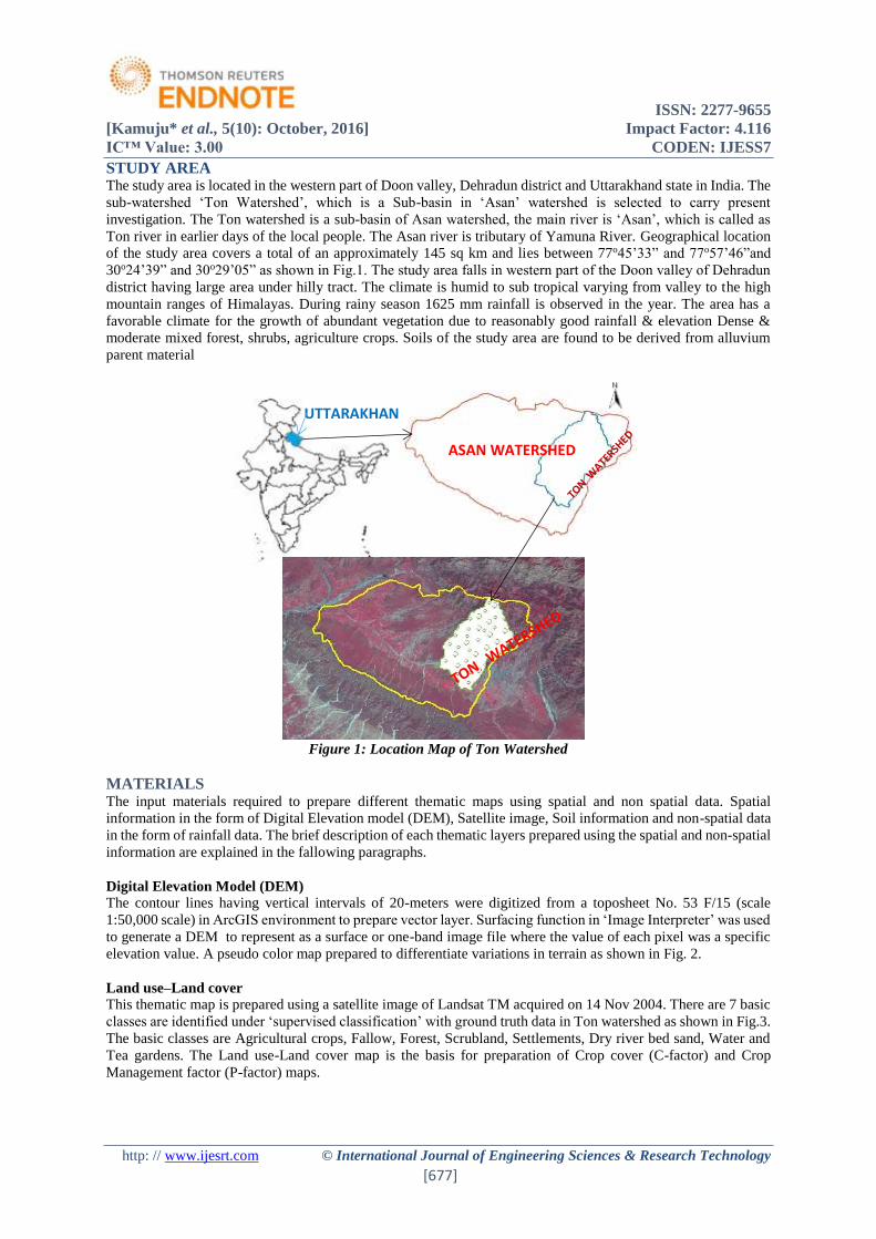
STUDY AREA The study area is located in the western part of Doon valley, Dehradun district and Uttarakhand state in India. The
sub-watershed ‘Ton Watershed’, which is a Sub-basin in ‘Asan’ watershed is selected to carry present
investigation. The Ton watershed is a sub-basin of Asan watershed, the main river is ‘Asan’, which is called as
Ton river in earlier days of the local people. The Asan river is tributary of Yamuna River. Geographical location
of the study area covers a total of an approximately 145 sq km and lies between 77o45’33” and 77o57’46”and
30o24’39” and 30o29’05” as shown in Fig.1. The study area falls in western part of the Doon valley of Dehradun
district having large area under hilly tract. The climate is humid to sub tropical varying from valley to the high
mountain ranges of Himalayas. During rainy season 1625 mm rainfall is observed in the year. The area has a
favorable climate for the growth of abundant vegetation due to reasonably good rainfall & elevation Dense &
moderate mixed forest, shrubs, agriculture crops. Soils of the study area are found to be derived from alluvium
parent material
Figure 1: Location Map of Ton Watershed
MATERIALS The input materials required to prepare different thematic maps using spatial and non spatial data. Spatial
information in the form of Digital Elevation model (DEM), Satellite image, Soil information and non-spatial data
in the form of rainfall data. The brief description of each thematic layers prepared using the spatial and non-spatial
information are explained in the fallowing paragraphs.
Digital Elevation Model (DEM)
The contour lines having vertical intervals of 20-meters were digitized from a toposheet No. 53 F/15 (scale
1:50,000 scale) in ArcGIS environment to prepare vector layer. Surfacing function in ‘Image Interpreter’ was used
to generate a DEM to represent as a surface or one-band image file where the value of each pixel was a specific
elevation value. A pseudo color map prepared to differentiate variations in terrain as shown in Fig. 2.
Land use–Land cover
This thematic map is prepared using a satellite image of Landsat TM acquired on 14 Nov 2004. There are 7 basic
classes are identified under ‘supervised classification’ with ground truth data in Ton watershed as shown in Fig.3.
The basic classes are Agricultural crops, Fallow, Forest, Scrubland, Settlements, Dry river bed sand, Water and
Tea gardens. The Land use-Land cover map is the basis for preparation of Crop cover (C-factor) and Crop
Management factor (P-factor) maps.
UTTARAKHAND
ASAN WATERSHED

ISSN: 2277-9655
[Kamuju* et al., 5(10): October, 2016] Impact Factor: 4.116
IC™ Value: 3.00 CODEN: IJESS7
http: // www.ijesrt.com © International Journal of Engineering Sciences & Research Technology
[678]
Figure 2: DEM of Ton watershed Figure 3: Land Use – Land Cover Map of Ton
Watershed
Soil data
This data collected form textural properties of soils covered in the watershed. A polygonised soil map prepared
based on the types of soils covered in the catchment as shown in Fig.4. There are 6 verities of soil textural classes
are identified from ‘Ton’ sub-basin. These are Loam, Silt Loam, Sandy Loam, Sandy clay Loam, Gravelly clay
loam, Loam to Sandy Clay Loam. The higher portion of the catchment covered with Loamy soils and a least area
of soils are covered with loam to sandy clay loam.
Rainfall data
Rainfall data collected from rain gauge stations available in the Ton watershed. In order to prepare R-factor map,
rainfall data available from a Self recording rain gauges at Poanta Sahib village. From the average annual rainfall,
‘R-factor’ is calculated from raster calculator available in spatial analyst tool in ArcGIS environment. The rain
gauge available in the watershed is shown in Fig.5
Figure 4: Soil Map of Ton Watershed Figure 5: Rain gauge Location of Ton Watershed
ISSN: 2277-9655
[Kamuju* et al., 5(10): October, 2016] Impact Factor: 4.116
IC™ Value: 3.00 CODEN: IJESS7
http: // www.ijesrt.com © International Journal of Engineering Sciences & Research Technology
[679]
METHODOLOGY In this study, a remote Sensing and GIS integrated RUSLE equation and GIS based Hydrological model of
‘SATEEC GIS system’ were used to estimate spatial soil erosion of the Ton watershed. These models are utilized
a common equation for computation of soil erosion. The RUSLE predicts Average annual soil loss for a given site
as a product of six major erosion factors (equation 1), whose values at a particular location can be expressed
numerically.
A = R * K * L * S * C * P ……………….Eqn…….(1)
Where,
A : computed annual soil loss per unit area [ton/ha/year]
R: Rainfall erosivity factor, an erosion index for the given storm period in [MJ mm·ha−1·hr−1·year−1]
K: Soil erodibility factor (soil loss per erosion index unit for a specified soil measured on a standard plot,
22.1 m long, with uniform 9% (5.16°) slope, in continuous tilled fallow) [ton·ha·hr·ha−1·MJ−1·mm−1].
L: Slope length factor (ratio of soil loss from the field slope length to soil loss from standard 22.1 m slope under
identical conditions)
S: Slope steepness factor-Ratio of soil loss from the field slope to that from the standard slope under identical
conditions
C: Cover-management factor-Ratio of soil loss from a specified area with specified cover and management to
that
from the same area in tilled continuous fallow
P:Support practice factor-Ratio of soil loss with a support practice contour tillage, strip-cropping, terracing to soil
loss with row tillage parallel to the slope.
L,S,C,P factors are dimensionless parameters and they are normalized relative to standard plot conditions. The
USLE and RUSLE is currently a globally accepted method for soil erosion prediction in the US and in other
countries all over the world. These models have been accepted to be useful, accurate and reliable. In the present
study, annual soil loss rates and severity were computed based on RUSLE in GIS environment using Arc GIS 9.3
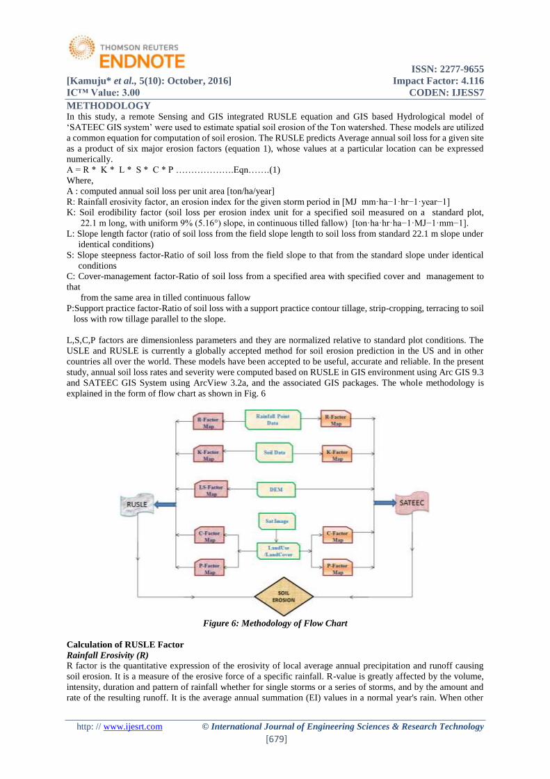
and SATEEC GIS System using ArcView 3.2a, and the associated GIS packages. The whole methodology is
explained in the form of flow chart as shown in Fig. 6
Figure 6: Methodology of Flow Chart
Calculation of RUSLE Factor
Rainfall Erosivity (R)
R factor is the quantitative expression of the erosivity of local average annual precipitation and runoff causing
soil erosion. It is a measure of the erosive force of a specific rainfall. R-value is greatly affected by the volume,
intensity, duration and pattern of rainfall whether for single storms or a series of storms, and by the amount and
rate of the resulting runoff. It is the average annual summation (EI) values in a normal year's rain. When other

ISSN: 2277-9655
[Kamuju* et al., 5(10): October, 2016] Impact Factor: 4.116
IC™ Value: 3.00 CODEN: IJESS7
http: // www.ijesrt.com © International Journal of Engineering Sciences & Research Technology
[680]
factors are constant, storm losses from rainfall are directly proportional to the product of the total kinetic energy
of the storm (E) times its maximum 30-minute intensity (I). Storms less than 0.5 inches are not included in the
erosivity computations because these storms generally add little to the total R value. R factors represent the
average storm EI values over a 22-year record. R is an indication of the two most important characteristics of a
storm determining its erosivity: amount of rainfall and peak intensity sustained over and extended period.
Rambabu et al. [12] developed a relationship between EI30 and daily and monthly rainfall amounts for Dehradun
(India) region as given below:
EI30 = 3.1 + 0.533 * Rd (for daily rainfall in mm)
EI30 = 1.9 + 0.640 * Rm (for monthly rainfall in mm)
Based on regression equation, R can be determined as follows:
R = 22.8 + 0.6400 * Ra
where,
R = Rainfall erosivity factor (in metric unit), and
Ra = Annual rainfall (mm)
This point information can be converted to spatial distribution by IDW method in GIS environment. Once this R
factor map is derived then by above formula, R factor map can be drawn and is shown in Fig.7
Soil Erodability Factor (K)
K factor is soil erodibility factor which represents both susceptibility of soil to erosion and the rate of runoff, as
measured under the standard unit plot condition. Soils high in clay have low K values, about 0.05 to 0.15, because
they resistant to detachment. Coarse textured soils, such as sandy soils, have low K values, about 0.05 to 0.2,
because of low runoff even though these soils are easily detached. Medium textured soils, such as the silt loam
soils, have a moderate K values, about 0.25 to 0.4, because they are moderately susceptible to detachment and
they produce moderate runoff. Soils having a high silt content are most erodible of all soils. They are easily
detached tend to crust and produce high rates of runoff. Values of K for these soils tend to be greater than 0.4.
Organic matter reduces erodibility because it reduces the susceptibility of the soil to detachment, and it increases
infiltration, which reduce runoff and thus erosion. Extrapolation of the K factor nomograph beyond an organic
matter of 4% is not recommended or allowed in RUSLE [13]. Soil structures affects both susceptibility to
detachment and infiltration. Permeability of the soil profile affects K because it affects runoff. The maps were
generated using the Inverse Distance Weighted (IDW) interpolation method on point data (vector layers) as shown
in Fig: 8. Therefore, the map was adopted to apply it in the RUSLE model.
Figure 7: R-factor Map of Ton Watershed Figure 8: K-factor Map of Ton Watershed
Slope Length and Steepness Factor (LS)
The (LS) factor expresses the effect of local topography on soil erosion rate, combining effects of slope length
(L) and slope steepness (S). Thus, LS is the predicted ratio of soil loss per unit area from a field slope from a 22.1
m long, 9% (5.16°) slope under otherwise identical conditions. L factor and S factor are usually considered
together.

ISSN: 2277-9655
[Kamuju* et al., 5(10): October, 2016] Impact Factor: 4.116
IC™ Value: 3.00 CODEN: IJESS7
http: // www.ijesrt.com © International Journal of Engineering Sciences & Research Technology
[681]
L is the slope length factor, representing the effect of slope length on erosion. It is the ratio of soil loss from the
field slope length to that from a 72.6-foot (22.1-meter) length on the same soil type and gradient. Slope length is
the distance from the origin of overland flow along its flow path to the location of either concentrated flow or
deposition. Slope lengths are best determined by visiting the site, pacing out flow paths, and making measurements
directly on the ground. Slope length values are generally too long when contour maps are used to choose slope
length. The main areas of deposition that end RUSLE slope length are at the base of concave slopes. If no signs
of deposition are present, the user will have to visualize where deposition occurs. The slope-ending depositional
area on a concave slope is usually below where the slope begins to flatten. Another difficulty is determining if a
channel is a concentrated flow channel that ends a RUSLE slope length. Channels that collect the flow from
numerous rills are generally considered to be slope ending concentrated flow channels.
S is the slope steepness. Represents the effect of slope steepness on erosion. Soil loss increases more rapidly with
slope steepness than it does with slope length. It is the ratio of soil loss from the field gradient to that from a 9
percent slope under otherwise identical conditions. The relation of soil loss to gradient is influenced by density of
vegetative cover and soil particle size
Figure 9: LS factor map for RUSLE Model Figure 10: LS factor map for SATEEC Model
The Digital Elevation Model (DEM) with a resolution of 20 m was used to calculate combined ‘LS’ factor map
for RUSLE model (Fig: 9) and SATEEC GIS system (Fig:10). However, Zhang et al. [14] developed more
accurate method to calculate the LS factor to estimate soil erosion at regional landscape scale. In this study both
RUSLE equation and SATEEC GIS system computes the LS factor using Moore and Burch [15] equation as given
below.
LS = (A
22.13)
0.6
X (sin θ
22.13)
1.3
Where
A : Flow Accumulation, and sin (θ) is slope of the watershed
Crop Management Factor (C)
The C-factor is used to reflect the effect of cropping and management practices on erosion rates. It is the factor
used most often to compare the relative impacts of management options on conservation plans. The crop
management factor expresses the effect of cropping and management practices on the soil erosion rate [16], and
is considered the second major factor (after topography) controlling soil erosion. An increase in the cover factor
indicates a decrease in exposed soil, and thus an increase in potential soil loss. RUSLE accounts for surface
roughness in the C value calculation. Surface roughness ponds water in depressions and reduces erosivity of
raindrop impact and water flow. If a C factor of 0.15 represents the specified cropping management system, it
signifies that the erosion will be reduced to 15 percent of the amount that would have occurred under continuous
ISSN: 2277-9655
[Kamuju* et al., 5(10): October, 2016] Impact Factor: 4.116
IC™ Value: 3.00 CODEN: IJESS7
http: // www.ijesrt.com © International Journal of Engineering Sciences & Research Technology
[682]
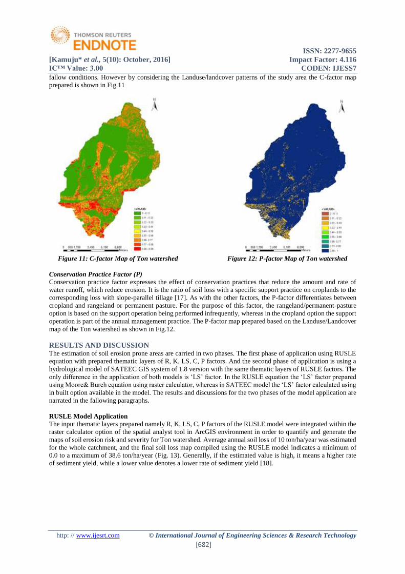
fallow conditions. However by considering the Landuse/landcover patterns of the study area the C-factor map
prepared is shown in Fig.11
Figure 11: C-factor Map of Ton watershed Figure 12: P-factor Map of Ton watershed
Conservation Practice Factor (P) Conservation practice factor expresses the effect of conservation practices that reduce the amount and rate of
water runoff, which reduce erosion. It is the ratio of soil loss with a specific support practice on croplands to the
corresponding loss with slope-parallel tillage [17]. As with the other factors, the P-factor differentiates between
cropland and rangeland or permanent pasture. For the purpose of this factor, the rangeland/permanent-pasture
option is based on the support operation being performed infrequently, whereas in the cropland option the support
operation is part of the annual management practice. The P-factor map prepared based on the Landuse/Landcover
map of the Ton watershed as shown in Fig.12.
RESULTS AND DISCUSSION The estimation of soil erosion prone areas are carried in two phases. The first phase of application using RUSLE
equation with prepared thematic layers of R, K, LS, C, P factors. And the second phase of application is using a
hydrological model of SATEEC GIS system of 1.8 version with the same thematic layers of RUSLE factors. The
only difference in the application of both models is ‘LS’ factor. In the RUSLE equation the ‘LS’ factor prepared
using Moore& Burch equation using raster calculator, whereas in SATEEC model the ‘LS’ factor calculated using
in built option available in the model. The results and discussions for the two phases of the model application are
narrated in the fallowing paragraphs.
RUSLE Model Application
The input thematic layers prepared namely R, K, LS, C, P factors of the RUSLE model were integrated within the
raster calculator option of the spatial analyst tool in ArcGIS environment in order to quantify and generate the
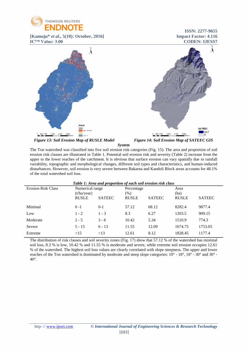
maps of soil erosion risk and severity for Ton watershed. Average annual soil loss of 10 ton/ha/year was estimated
for the whole catchment, and the final soil loss map compiled using the RUSLE model indicates a minimum of
0.0 to a maximum of 38.6 ton/ha/year (Fig. 13). Generally, if the estimated value is high, it means a higher rate
of sediment yield, while a lower value denotes a lower rate of sediment yield [18].
ISSN: 2277-9655
[Kamuju* et al., 5(10): October, 2016] Impact Factor: 4.116
IC™ Value: 3.00 CODEN: IJESS7
http: // www.ijesrt.com © International Journal of Engineering Sciences & Research Technology
[683]
Figure 13: Soil Erosion Map of RUSLE Model Figure 14: Soil Erosion Map of SATEEC GIS
System
The Ton watershed was classified into five soil erosion risk categories (Fig. 15). The area and proportion of soil
erosion risk classes are illustrated in Table 1. Potential soil erosion risk and severity (Table 2) increase from the
upper to the lower reaches of the catchment. It is obvious that surface erosion can vary spatially due to rainfall
variability, topographic and morphological changes, different soil types and characteristics, and human-induced
disturbances. However, soil erosion is very severe between Bakarna and Kandoli Block areas accounts for 48.1%
of the total watershed soil loss.
Table 1: Area and proportion of each soil erosion risk class
Erosion Risk Class Numerical range
(t/ha/year)
Percentage
(%)
Area
(ha)
RUSLE SATEEC RUSLE SATEEC RUSLE SATEEC
Minimal 0 -1 0-1 57.12 68.12 8282.4 9877.4
Low 1 - 2 1 - 3 8.3 6.27 1203.5 909.15
Moderate 2 - 5 3 - 6 10.42 5.34 1510.9 774.3
Severe 5 - 15 6 - 13 11.55 12.09 1674.75 1753.05
Extreme >15 >13 12.61 8.12 1828.45 1177.4
The distribution of risk classes and soil severity zones (Fig. 17) show that 57.12 % of the watershed has minimal
soil loss, 8.3 % is low, 10.42 % and 11.55 % is moderate and severe, while extreme soil erosion occupies 12.61
% of the watershed. The highest soil loss values are clearly correlated with slope steepness. The upper and lower
reaches of the Ton watershed is dominated by moderate and steep slope categories: 10° - 18°, 18° - 30° and 30° -
40°.

ISSN: 2277-9655
[Kamuju* et al., 5(10): October, 2016] Impact Factor: 4.116
IC™ Value: 3.00 CODEN: IJESS7
http: // www.ijesrt.com © International Journal of Engineering Sciences & Research Technology
[684]
Figure15: Spatial distribution of erosion risk categories Figure 16: Spatial distribution of
erosion risk
Using RUSLE Model categories Using SATEEC Model
SATEEC GIS System Application The thematic layers of R,K,C,P,DEM and boundary of the catchment are utilized as input to the SATEEC GIS
system. After DEM initialization, the LS factor map prepared using Moore & Burch for further process. The final
soil loss map compiled using the SATEEC GIS System model indicates a minimum of 0.0 to a maximum of 23.7
ton/ha/year (Fig. 14). The Ton watershed was classified into five soil erosion risk categories (Fig. 16). The area
and proportion of soil erosion risk classes are illustrated in Table 1. Potential soil erosion risk and severity (Table
2) increase from the upper to the lower reaches of the catchment similar fashion of RUSLE model. The distribution
of risk classes and soil severity zones (Fig. 18) show that 68.12 % of the watershed has minimal soil loss, 6.27 %
is low, 5.34% and 12.09 % is moderate and severe, while extreme soil erosion occupies 8.12 % of the watershed.
Figure 17: Spatial Distribution of Potential Figure 18: Spatial Distribution of Potential
Soil Risk Zones-RUSLE Model Soil Risk Zones –SATEEC Model

ISSN: 2277-9655
[Kamuju* et al., 5(10): October, 2016] Impact Factor: 4.116
IC™ Value: 3.00 CODEN: IJESS7
http: // www.ijesrt.com © International Journal of Engineering Sciences & Research Technology
[685]
CONCLUSION The present study identified the occurrence of higher severity of soil erosion from RUSLE model for the Ton
watershed compared to SATEEC GIS model. The mean soil loss estimated for the Ton watershed was 10
ton/ha/year, with the five erosion risk classes, ranging from 0.0 to 38.6 ton/ha/year and its corresponding areas of
82.824 km2 (8282.4 hectares) and 27.144 km2 (2714.4 hectares) were classed as low, moderate and 35.032 km2
(3503.2 hectares) are very severe soil erosion zones. Similarly, mean soil loss estimated for the Ton watershed
was 7.6 ton/ha/year, with the five erosion risk classes, ranging from 0.0 to 23.7 ton/ha/year from SATEEC GIS
system model and the areas of 98.774 km2 (9877.4 hectares) and 16.8345 km2 (1683.45 hectares) were classed as
suffering low to moderate and 29.3045 km2 (2930.45 hectares) are very severe soil erosion zones. The Remote
Sensing and GIS integrated RUSLE model denotes that Ton watershed larger area suffer soil erosion, and
SATEEC GIS model reveals lesser soil erosion risk. The graphical presentation of results of both models are
clearly shows the discrimination of erosion classes as shown in Fig.19. The overall results reveals that Ton
watershed suffer a very less area of the catchment suffer extreme erosion prone areas and most of the area comes
under non erosion prone zones.
Figure 19: Soil Erosion classes of RUSLE and SATEEC Models
Spatial analysis denoted high soil erosion rates in the upper and mid reaches of the catchment in both RUSLE and
SATEEC models. Here, long and continuous human disturbance and deforestation, with the combined effect of
K, LS, and C factors, account for high soil erosion loss across the study area. Accordingly, soil erosion becoming
more serious on moderate and steep slopes transformed into cultivated or range land. Therefore, the expansion of
cultivated cereals increase the susceptibility of soils to erosion, and the cultivated lands with poor conservation
measure exhibit higher rate of soil erosion and decline in soil fertility.
It is postulated elsewhere that the RUSLE parameters can be altered significantly by human activities [13]. The C
and P factors can be improved to reduce the soil erosion loss through afforestation and shifting community
environmental practice. The LS factor also can be modified by shortening the length and steepness of slopes by
the construction of contour walls and stone terraces. Construction of soil conservation measures is vital to control
runoff and soil erosion across different agro ecological zones and under various land uses. More data on rainfall
and its duration and intensity provided a basis for calculating erosive of rainfall. Field measurements of rainfall
erosion in the form of direct measurements and simulated rainfall are highly recommended. Finally, the present
investigation has demonstrated that GIS and RS techniques are simple and low-cost tools for modeling soil
erosion, with the purpose of assessing erosion potential and risk for the watersheds of Uttarakhand regional
watersheds.
ACKNOWLEDGEMENTS I am very much thankful to CWPRS to allow me to carry research on this topic of my interest. Also thankful to
the Korean society of Agricultuyre Enginners to develop and supply of the software ‘SATEEC GIS system’ to the

ISSN: 2277-9655
[Kamuju* et al., 5(10): October, 2016] Impact Factor: 4.116
IC™ Value: 3.00 CODEN: IJESS7
http: // www.ijesrt.com © International Journal of Engineering Sciences & Research Technology
[686]
public.
REFERENCES [1] European Environment Agency, 1995. CORINE soil risk and important land resources in the southern
regions of the European Community, Commission of the European Communities.
[2] Pimental, D., 1998. Ecology of soil erosion in ecosystems. Ecosystems (1),pp: 416-426.
[3] Morgan, R.P.C., 1995. Soil erosion and conservation. Longman, London, pp: 23-37.
[4] Moore, I.D. and J.P. Wilson, 1992. Length-slope factors for the Revised Universal Soil Loss Equation:
Simplified method of estimation. Journal of Soil and Water Conservation, 47: 423-428.
[5] Pandey, A., V.M. Chowdary and B.C. Mal, 2009. Sediment Yield Modelling of and Agricultural
Watershed Using MUSLE, Remote Sensing and GIS. J. Paddy Water Environment (Springer)., 7(2):
105-113.
[6] Wischmeier, W.H. and D.D. Smith, 1978. Predicting rainfall erosion. losses: a guide to conservation
planning. Agriculture Handbook, vol. 537. US Department of Agriculture, Washington,DC, pp: 58.
[7] Flanagan, D.C. and M.A. Nearing, 1995. USDA water erosion prediction project: hillslope profile and
watershed model documentation. NSERL Report No. 10. USDA-ARS National Soil Erosion Research
Laboratory, West Lafayette, IN 47907-1194.
[8] Arnold, J.G., R. Srinivasan, R.S. Muttiah and J.R. Williams, 1998. large area hydrologic modeling and
assessment: Part I. Model development. Journal of the American Water Resources Association, 34(1):
73-89.
[9] Morgan, R.P.C., J.N. Quinton, R.E. Smith, G. Govers, J. Poesen, K. Auerswald, G. Chisci, D. Torri. and
M.E. Styczen, 1998. The European Soil Erosion Model (EUROSEM): a dynamic approach for predicting
sediment transport from fields and small attachments.Earth Surface Processes and Landforms, 23: 527-
544.
[10] Renard, K.G., G.R. Foster, G.A. Weesies, J.P. Porter, 1991. RUSLE: revised universal soil loss equation.
Journal of Soil and Water Conservation, 46(1): 30-33.
[11] Lim, KJ., J. Choi, K. Kim, M. Sagong and B.A. Engel, 2003. Development of sediment assessment tool
for effective erosion control (SATEEC) in small scale watershed. Transactions of the Korean Society of
Agricultural Engineers, 45(5): 85-96.
[12] Rambabu, Tejwani, K.K., Agrawal, M.C. and Bhusan, L.S. 1979. Rainfall Intensity Duration-Return
Equation and Nomographs of India, CSWCRTI, ICAR, Dehradun, India.
[13] P.Mhangara, V. Kakembo and K. Lim, “Soil Erosion Risk Assessment of the Keiskamma Catchment,
South Africa Using GIS and Remote Sensing,” Environmental Earth Science, Vol. 65, No. 7, 2012,
pp.2087-2102. http://dx.doi.org/10.1007/s12665-011-1190-x
[14] H. Zhang, Q. Yang, R. Li, Q. Liu, D. Moore, P. He, C. Ritsema and V. Geissen, “Extension of a GIS
Procedure for Calculating the RUSLE Equation LS Factor,” Computers and Geoscences, Vol. 52, No. 1,
2013, pp. 177-188. http://dx.doi.org/10.1016/j.cageo.2012.09.027
[15] Moore, I. D. and Burch, G. J. 1986. Physical Basis of the Length-Slope Factor in the Universal Soil Loss
Equation. Soil Sci. Soc. Am. J. 50:1294-1298.
[16] K. G. Renard, G. R. Foster, G. A. Weesies, D. K. McCool and D. C. Yoder, “Predicting Soil Erosion by
Water: A Guide to Conservation SPlanning with the Revised Universal Soil Loss Equation (RUSLE),”
Agricultural Handbook No. 703, US Department of Agriculture,Washington DC, 1997.
[17] A.Rabia, “Mapping Soil Erosion Risk Using RUSLE, GIS and Remote Sensing Techniques,” 4th
International Congress of ECSSS, EUROSOIL, Bari, 2-6 June 2012, p.1082.
[18] V. Prasannakumar, H. Vijith, N. Geetha and R. Shiny, “Regional Scale Erosion Assessment of a Sub
Tropical High- land Segment in the Western Ghats of Kera, South India,” Water Resources Management,
Vol. 25, No. 14, 2011, pp. 3715-3727. http://dx.doi.org/10.1007/s11269-011-987-y


