
I. INTRODUCTION
We are modeling the processes by which increasing demand for developed land uses, brought about by changes in the regional economy and the socio-demographics of the region, is translated into a changing spatial pattern of land use. Our study focus is a portion of the Chesapeake Bay Watershed where the spatial patterns of sprawl represent a set of conditions generally prevalent in much of the U.S. Working in the region permits access to:
a time-series of multi-scale and multi-temporal (including historical) satellite imagery, andan established network of collaborating partners and agencies willing to share resources and eager to utilize developed techniques and model results.
Once accomplished, predictions of future land use change can permit scenario analyses of future carbon dynamics as well as nutrient loadings into the Chesapeake Bay tributaries. It can also provide critical quantitative insight into the impact of alternative land management and policy decisions, since one of the states in the region (Maryland) is a leader in adopting "Smart Growth" policies which are aimed at curbing sprawl development. Our technical approach includes three components:
spatial econometric modeling of the development decision, advanced remote sensing of suburban change and residential land use density, including comparisons of past change from Landsat analyses and more traditional sources, andlinkages between the two through variable initialization and supplementation of parcel level data
We have also investigated predictive urban modeling with a cellular automata (CA) based model, SLEUTH. By comparing the CA approach to the econometric approach, we have identified the major strengths and weaknesses of each modeling technique. This will allow us to work toward an integrated modeling framework that is applicable to broader scales, yet incorporates fine scale economic and demographic information.
Model of housing starts as function of regional economic projections
Historic rates and patterns of developmentSource of growth pressure
information
Parcel level data including locations of parcels, GIS data on physical features, regulations, public goods, land cover
Urban extent data for at least 4 points in time; road networks for 2 points in time; excluded layers for calibration and predictive scenarios
Data required
Discrete choice or hazard model analysis to test hypotheses and calibrate parameter estimates for forecasting
Cellular automata models that simulate cell changes by an iterative calibration process using observed cell changes
Analytical Method
Value of land in undeveloped use, value of land in developed uses, and conversion costs. All are functions of: current land cover, physical and locational features, public goods provision, and relevant regulations
State of current land cover, physical features of the landscape, user-defined areas that are protected from development.
“Driving Forces”
Stochastic model of behavior of land owners (choosing optimal timing of development and optimal density of development)
Stochastic process regulated by conceptually simple transition rules. SLEUTH employs “slope”, “spread”, “breed”, “dispersion”, and “road gravity” coefficients
Nature of land use change process
Process-basedPattern-basedNature of ApproachPrivately owned parcel of landCell in landscape Unit of Observation
Economic Modeling Cellular Automaton Modeling (e.g. Sleuth)
IV. COMPARISON OF MODELING APPROACHES
The econometric approach is robust, yet data intensive and therefore difficult to extend over a region such as the Mid-Atlantic. Methods to incorporate remote sensing data as model input are being developed and could decrease the need for detailed parcel data. The CA model is less data intensive and relies on data sets that are potentially available over large areas. Assumptions concerning growth processes are, however, highly simplified in this approach. Because the microeconomic modeling system attempts to model processes rather than patterns or trends, it is more successful at capturing low density development patterns. Knowledge of the development process gained through the application of econometric modeling could be incorporated into the CA platform, creating an integrated modeling framework.
II. ECONOMIC MODELING
This approach to land use change modeling estimates parameters of decisions made by parcel owners (agents) regarding the optimal timing and density of development, taking into account market and regulatory constraints The increased fragmentation of land uses and growth in low density residential uses requires improved methods of predicting spatial patterns of change. This work takes advantage of parcel level geocoded data, specifically recognizes heterogeneity in space, and incorporates spatial interactions of land use change (Figure 1).
Spatial Predictive Modeling and Remote Sensing of Land Use Changein the Chesapeake Bay Watershed
Scott J. GoetzWoods Hole Research Center
Nancy E. BockstaelUniversity of [email protected]
Table 1: Comparison of modeling approaches
REFERENCESBockstael N E, 1996, "Modeling Economics and Ecology: the Importance of a Spatial Perspective" American Journal of Agriculture and Economics 78 5 1168-1180Chesapeake Bay Program, 2000, “Chesapeake 2000”, http://www.chesapeakebay.net/agreement.htmClarke K C, Hoppen S, Gaydos L, 1997, "A Self-modifying Cellular Automaton Model of Historical Urbanization in the San Francisco Bay Area" Environment and Planning B: Planning and Design 24 247-261Jantz C A, Goetz S J, Shelley M K, in press, "Using the SLEUTH Urban Growth Model to Simulate the Impacts of Future Policy Scenarios on Urban Land Use in the Baltimore-Washington Metropolitan Area" Environment and Planning B: Planning and Design US Geological Survey, 2002, "Project Gigalopolis: Urban and Land Cover Modeling", http://www.ncgia.ucsb.edu/projects/gig/v2/Home/home.htm
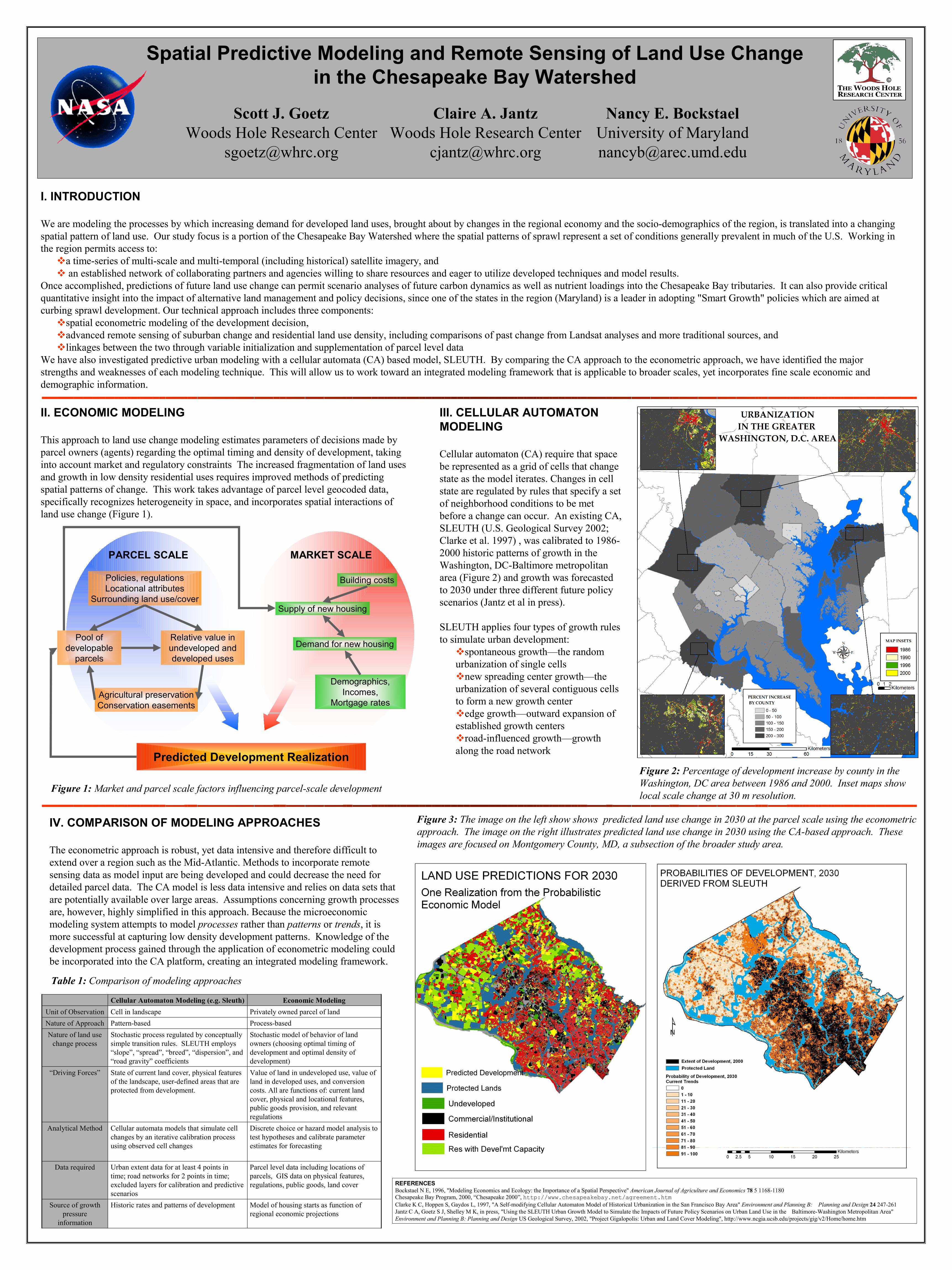
III. CELLULAR AUTOMATON MODELING
Cellular automaton (CA) require that space be represented as a grid of cells that change state as the model iterates. Changes in cell state are regulated by rules that specify a set of neighborhood conditions to be met before a change can occur. An existing CA, SLEUTH (U.S. Geological Survey 2002; Clarke et al. 1997) , was calibrated to 1986-2000 historic patterns of growth in the Washington, DC-Baltimore metropolitan area (Figure 2) and growth was forecasted to 2030 under three different future policy scenarios (Jantz et al in press).
SLEUTH applies four types of growth rules to simulate urban development:
spontaneous growth—the random urbanization of single cells
new spreading center growth—the urbanization of several contiguous cells to form a new growth center
edge growth—outward expansion of established growth centers
road-influenced growth—growth along the road network
Figure 2: Percentage of development increase by county in the Washington, DC area between 1986 and 2000. Inset maps show local scale change at 30 m resolution.
PARCEL SCALE MARKET SCALE
Policies, regulationsLocational attributes
Surrounding land use/cover
Pool of developable
parcels
Relative value in undeveloped and developed uses
Agricultural preservationConservation easements
Building costs
Supply of new housing
Demand for new housing
Demographics, Incomes,
Mortgage rates
Predicted Development Realization
Figure 1: Market and parcel scale factors influencing parcel-scale development
Figure 3: The image on the left show shows predicted land use change in 2030 at the parcel scale using the econometric approach. The image on the right illustrates predicted land use change in 2030 using the CA-based approach. These images are focused on Montgomery County, MD, a subsection of the broader study area.
Claire A. JantzWoods Hole Research Center


