

Special cycles on Shimura curves and the Shimura lift
by
Siddarth Sankaran
A thesis submitted in conformity with the requirementsfor the degree of Doctor of PhilosophyGraduate Department of Mathematics
University of Toronto
Copyright c© 2012 by Siddarth Sankaran
Abstract
Special cycles on Shimura curves and the Shimura lift
Siddarth Sankaran
Doctor of Philosophy
Graduate Department of Mathematics
University of Toronto
2012
The main results of this thesis describe a relationship between two families of arithmetic divisors on an
integral model of a Shimura curve. The first family, studied by Kudla, Rapoport and Yang, parametrizes
abelian surfaces with specified endomorphism structure. The second family is comprised of pullbacks of
arithmetic cycles on integral models of Shimura varieties associated to unitary groups of signature (1,1).
In the thesis, we construct these families of cycles, and describe their relationship, which is expressed in
terms of the “Shimura lift”, a classical tool in the theory of modular forms of half-integral weight. This
relations can be viewed as further evidence for the modularity of generating series of arithmetic ”special
cycles” for U(1,1), and fits broadly into Kudla’s programme for unitary groups.
ii

Dedication
This thesis is dedicated to the memory of my father, Pancha Sankaran. I may not be quite the sort of
doctor he had hoped for, but I’m sure he’d be proud regardless.
Acknowledgements
First and foremost, I would like to thank my advisor, Stephen S. Kudla. His constant and consistent
encouragement, and keen mathematical insight, have been inspirational; I am very grateful for all that
he has taught me.
I also wish to thank Benjamin Howard, Brian Smithling, Ulrich Terstiege, Patrick Walls, and Ying
Zong for several illuminating, and often timely, conversations. Most of the work in this thesis is modelled
on work of Howard, Kudla, Rapoport, Shimura, Terstiege, and Yang; I would like to thank them for
teaching me the tools of the trade. In addition, I would like to acknowledge Benjamin Howard once
again, for providing detailed and very helpful comments on a previous version of this thesis.
A special thank you to Ida Bulat, for smoothing out all the bureaucratic wrinkles with seemingly
infinite patience and good cheer.
Finally, thanks to my family and friends, especially Geethuma and Sandrina, for all the love and the
laughs over the years.
iii

Contents
1 Introduction 1
1.1 Outline of the thesis . . . . . . . . . . . . . . . . . . . . . . . . . . . . . . . . . . . . . . . 5
1.2 Notation . . . . . . . . . . . . . . . . . . . . . . . . . . . . . . . . . . . . . . . . . . . . . . 7
2 Shimura curves and orthogonal special cycles 9
2.1 Intersection theory for arithmetic surfaces . . . . . . . . . . . . . . . . . . . . . . . . . . . 9
2.2 A decomposition of CH1(X )R . . . . . . . . . . . . . . . . . . . . . . . . . . . . . . . . . . 12
2.3 Shimura curves . . . . . . . . . . . . . . . . . . . . . . . . . . . . . . . . . . . . . . . . . . 14
2.4 Orthogonal special cycles . . . . . . . . . . . . . . . . . . . . . . . . . . . . . . . . . . . . 16
2.5 The Hodge class . . . . . . . . . . . . . . . . . . . . . . . . . . . . . . . . . . . . . . . . . 18
2.6 The generating series of orthogonal special cycles . . . . . . . . . . . . . . . . . . . . . . . 18
3 Unitary Shimura varieties and special cycles 21
3.1 The global moduli problem . . . . . . . . . . . . . . . . . . . . . . . . . . . . . . . . . . . 21
3.2 Unitary special cycles . . . . . . . . . . . . . . . . . . . . . . . . . . . . . . . . . . . . . . 22
3.3 Complex uniformizations of Md and special cycles . . . . . . . . . . . . . . . . . . . . . . 24
3.4 The Hodge class . . . . . . . . . . . . . . . . . . . . . . . . . . . . . . . . . . . . . . . . . 27
3.5 Green functions for unitary special cycles . . . . . . . . . . . . . . . . . . . . . . . . . . . 28
4 The classical Shimura lift via theta series 32
5 The main results 39
5.1 Pullbacks of special cycles to Shimura curves . . . . . . . . . . . . . . . . . . . . . . . . . 39
5.2 Unitary generating series, and statement of the main theorems . . . . . . . . . . . . . . . 40
5.3 Some remarks on the constant term . . . . . . . . . . . . . . . . . . . . . . . . . . . . . . 44
iv

6 Mordell-Weil and degQ components 47
6.1 Conductors of embeddings, orders, and special cycles . . . . . . . . . . . . . . . . . . . . . 47
6.2 Local Frobenius types of special endomorphisms . . . . . . . . . . . . . . . . . . . . . . . 51
6.3 The complex points of the pullback of a unitary special cycle . . . . . . . . . . . . . . . . 53
7 Analytic components 64
8 Vertical components 73
8.1 Dieudonne modules and deformations of p-divisible groups . . . . . . . . . . . . . . . . . . 73
8.2 Cycles in moduli spaces of p-divisible groups . . . . . . . . . . . . . . . . . . . . . . . . . 77
9 The Hodge component 106
v

Chapter 1
Introduction
The main theorems of this thesis exhibit a relationship between two families of divisors that live on an
integral model of a Shimura curve. The first family was introduced and studied by Kudla, Rapoport,
and Yang, while the second family arose from a more recent investigation of Kudla and Rapoport
regarding cycles on integral models of Shimura varieties associated to unitary groups. The present work
demonstrates that these two families, when expressed as the coefficients in formal generating series, are
related by an arithmetic-geometric version of the Shimura lift, a classical tool in the theory of modular
forms.
The divisors occurring in these two families are examples of so-called “special” rational cycles on Shimura
varieties, which have been the focus of extensive study in the past few decades. In particular, a recurring
phenomenon has emerged whereby in many cases intersection numbers of these cycles are related to the
Fourier coefficients of modular forms. This relationship is perhaps not altogether unexpected, as the
construction of these cycles has some of the flavour of the theory of theta series; on the other hand, a
general theory that adequately addresses the phenomena that have been observed, in particular regarding
the arithmetic aspects of the theory, is highly elusive.
A prototypical result is contained in work of Hirzebruch and Zagier [7], in which the authors construct
a formal generating series whose terms are cohomology classes of curves on a Hilbert modular surface,
which are represented by certain embedded rational sub-Shimura varieties. They then prove that this
generating series is modular ; namely, after applying any linear functional to the coefficients, the resulting
generating series is the Fourier expansion of a modular form.
1

Chapter 1. Introduction 2
By utilizing the theory of theta correspondences and the Weil representation, Kudla and Millson [11] were
able to give a more conceptual explanation for, and vast generalization of, the theorem of Hirzebruch and
Zagier; they prove the modularity of generating series valued in the cohomology of arithmetic quotients
of hermitian symmetric domains associated to unitary and orthogonal groups of arbitrary signature.
In another direction, Borcherds [1] proves an analogous statement for generating series of divisors in
Chow groups of Shimura varieties associated to orthogonal groups O(n, 2), by constructing a sufficiently
large supply of meromorphic modular forms. It is worth noting that his approach also hinges upon an
application of the Weil representation.
In certain cases, one can define tractable integral models for such Shimura varieties and the special
cycles, which arise in practice via moduli problems for abelian varieties with additional (polarization and
endomorphism) structure. In this setting, one can form the analogous generating series with coefficients
in arithmetic (Arakelov) Chow groups, and ask whether it is the Fourier expansion of a modular form.
Although the rather more complicated structure of arithmetic Chow groups precludes a general theory
for such generating series, we shall discuss two examples that have afforded profitable investigation, and
which are the point of departure for this thesis.
In a series of works culminating in the monograph [17], Kudla, Rapoport and Yang investigate a gen-
erating series of arithmetic special cycles on CB, an integral model of a Shimura curve associated to a
quaternion algebra over the rational numbers. The “special cycles” in this setting are divisors that are
the (arithmetic) analogues of complex multiplication points on modular curves. The first main theorem
of [17], which we shall discuss in greater detail in Chapter 2, asserts that for τ = u + iv ∈ H, this
generating series
Φo(τ) =∑n∈ZZo(n, v) qn, q = e2πiτ , (1.1)
is the q-expansion of a modular form of weight 3/2, with coefficients Zo(n, v) valued in the first arithmetic
Chow group CH1(CB)R (here and throughout, we take our arithmetic Chow groups with real coefficients).
More recently, Kudla and Rapoport [13, 14] have described integral models for Shimura varieties for
unitary groups U(p, q) of arbitrary signature over an imaginary quadratic field k, as well as special cycles
occurring in all codimensions of the form qr, 0 ≤ r ≤ p. They also prove that in the case of signature
(p, 1), certain intersection multiplicities of the special cycles are given by the Fourier coefficients of a
derivative of an Eisenstein series. Results in this vein, which can also be found in e.g. [8, 23], provide
evidence for the modularity of a conjectural generating series of special cycles valued in the arithmetic
Chow groups, in analogy with the Shimura curve case above; however, as these moduli spaces and their

Chapter 1. Introduction 3
Chow groups are rather more complicated than before, such a theorem is still out of reach for general
unitary groups. In fact, as these spaces are often non-proper, it is not even clear how to define the Green
currents for the special cycles which are needed in order to construct arithmetic cycles at this level of
generality.
In this thesis, we discuss a variant of the unitary Shimura variety of Kudla and Rapoport in the case of
signature (1, 1), defined as a moduli space M of polarized abelian surfaces with complex multiplication
by k; in contrast to the spaces discussed in [14], our space M parametrizes polarizations that are non-
principal. We also describe the construction of a family of “unitary” special cycles in M, which we
denote by Z(m), for m ∈ Z; see Chapter 3.
Suppose B is an indefinite rational quaternion algebra, and OB a maximal order. If k is an imaginary
quadratic field, with ring of integers ok, we show (c.f. Chapter 5) that any embedding φ : ok → OB
induces a morphism
φ : CB →M,
where CB is an integral model of a Shimura curve as described above.
We also discuss how to equip the pullback φ∗Z(m) of a unitary special cycle with an explicit Green’s
function φ∗Gr(m, v), depending on a real parameter v > 0. In this way, we obtain arithmetic classes
φ∗Z(m, v) = (φ∗Z(m), φ∗Gr(m, v)) ∈ CH1(CB)R
in the first arithmetic Chow group of CB (taken with real coefficients).
We then obtain a generating series, valued in CH1(CB)R, whose coefficients are given by the pullbacks
of the unitary special cycles:
φ∗Φ(τ) :=∑m∈Z
φ∗Z(m, v) qm. (1.2)
We also form a linear combination of such pullbacks
Φ∗(τ) :=1
h(k)|o×k |∑
[φi]∈Opt
∑m∈Z
φ∗i Z(m, v) qm, (1.3)
where h(k) is the class number of k, and the sum on φi runs over a set of representatives of optimal
embeddings φi : ok → OB, taken up to O×B -conjugacy, c.f. Chapter 5.
As we discuss in Chapter 2, the arithmetic Chow group of CB is equipped with a height pairing
〈·, ·〉 : CH1(CB)R × CH1(CB)R → R,

Chapter 1. Introduction 4
and admits a natural orthogonal decomposition into three subspaces
CH1(CB)R = MW ⊕An⊕ (R ωo ⊕ V ert), (1.4)
according to which we may decompose our generating series (1.1) and (1.3).
A more detailed outline of the main results in this thesis appears at the end of §5.2; for convenience, we
provide a brief summary here. We begin with the MW and An components:
Theorem. Let k = Q(√
∆) be an imaginary quadratic field, with ∆ < 0 a squarefree, even integer.
Let B denote a rational indefinite division quaternion algebra, such that all the primes at which B is
ramified are inert in k. Then we have equalities of q-expansions
(i) Sh|∆|(ΦoMW )(τ) = Φ∗MW (τ),
(ii) and Sh|∆|(ΦoAn)(τ) = Φ∗An(τ),
where Sh|∆| is the Shimura lift with parameter |∆|.
In particular, Φ∗MW (τ) and Φ∗An(τ) are modular forms of weight 2.
Turning to the third component in (1.4), it turns out that the subspace V ert (which stands for “vertical”)
is spanned by a “constant” class 1, together with classes Yp representing irreducible components of
the special fibres of CB at primes p of bad reduction. Moreover, for an arithmetic cycle Z ∈ CH1(CB)R,
we have
〈Z,1〉 =1
2degQ(Z),
where degQ(Z) denotes the degree of the generic fibre of Z.
In the course of proving part (i) of the above theorem, and under the same hypotheses, we also prove
the relation
degQ Φ∗(τ) = Sh|∆| degQ Φo(τ).
The proof of the corresponding formula for the Yp’s, however, is still in progress. The proof is carried out
in two stages: first, we consider an analogous problem relating families of orthogonal and unitary cycles
on Rapoport-Zink spaces, which are moduli spaces of p-divisible groups; we then relate these cycles to
the special fibres of the generating series Φ∗(τ) and Φo(τ) via p-adic uniformizations.
In Chapter 8, we carry out the first part of this program, which owing to recent work [13, 15] of Kudla
and Rapoport, is hopefully of sufficient independent interest.
Chapter 1. Introduction 5
Finally, in Chapter 9, we discuss the Shimura lift formula for the Hodge components, obtained by pairing
the coefficients of our two generating series with the “Hodge class” ωo appearing in (1.4). Each of these
pairings can be expressed as the sum of an Archimedean term, which involves the Green functions of the
cycles, and a geometric term.
We prove, again under the hypotheses of the main theorem, thatArchimedean contributions to
〈Sh|∆|Φo(τ), ωo〉
=
Archimedean contributions to
〈Φ∗(τ), ωo〉
We also demonstrate that the analogous statement for the geometric contributions follows from two
conjectures, namely (i) that the Shimura lift formula holds for the vertical components, as above, and
(ii) the cycles φ∗Z(m) have no irreducible components concentrated at primes of good reduction.
I would like to conclude the introduction with some speculative remarks.
The notation for the generating series (1.2) is intentionally suggestive; what one would hope to do is
define a generating series
Φu(w) =∑m∈ZZ(m, η) qmw ∈ CH1(Md)RJq±1
w K, (1.5)
directly onMd, and as conjectured by Kudla’s programme, show that it is the q-expansion of a modular
form. In particular, when d = DB , the generating series (1.2) would arise naturally via a morphism
φ∗ : CH1(MDB )R → CH1(CB)R.
The problem with this construction, as pointed out to me by Ben Howard, is that it is not at all clear
that the space Md is an arithmetic surface in the sense of Section 2.1, and so the theory of arithmetic
Chow groups developed there may not apply.
In this thesis, we circumvent this issue by defining the unitary cycles directly on the Shimura curve
CB, where the theory of arithmetic Chow groups does apply. If, however, one is able to overcome the
difficulties in making sense of the generating series (1.5), then one can interpret the main theorems of
this thesis as compelling evidence for its modularity.
1.1 Outline of the thesis
We begin Chapter 2 with a brief discussion of background material regarding arithmetic surfaces and
the structure of their first arithmetic Chow groups. We then review the construction of the integral

Chapter 1. Introduction 6
models of Shimura curves, and introduce our first family of special divisors, the “orthogonal generating
series” of Kudla, Rapoport and Yang. In particular, we make a note of their remarkable theorem that
this generating series is in fact a modular form weight 3/2.
In Chapter 3 we introduce the unitary moduli problem, which is a mild variant of the one introduced
by Kudla and Rapoport. We also describe the unitary special cycles, and their Green functions.
Chapter 4 consists of some background material regarding the Shimura lift, and specifically the version
considered by Niwa, in the classical setting; in particular, we develop a Poincare series expression that
will facilitate the explicit calculations in later chapters.
In Chapter 5 we construct our second generating series, which arises via pullbacks of unitary cycles
to a Shimura curve. We also give a precise statement of the main results, which relate this generating
series with the Shimura lift of the orthogonal one of Chapter 2.
In light of the results of Chapter 2, which describes a decomposition of the orthogonal generating
series into 5 components, we may compare the Shimura lift of each component with the corresponding
component of the unitary generating series. For each component, the strategy is along the same lines:
we apply the explicit formulas for the Shimura lift to the piece of the orthogonal generating series in
that component, and compare the result to the corresponding contribution from the unitary cycles.
For the degree and Mordell-Weil components, discussed in Chapter 6, we utilize descriptions of the
complex fibres of the cycles in terms of arithmetic quotients of symmetric spaces. The question then
boils down to an algebraic one, namely a counting argument for the number of elements of certain norm
in the centralizer of an element of a quaternion algebra; the expressions that result turn out to coincide
with the Fourier coefficients of the Shimura lift of a holomorphic modular form, which allows to prove
the Shimura lift formula in this case.
The proof for the analytic components, found in Chapter 7, hinges on the particular choices of Green
functions that were made; in particular, we make use of the explicit formulation of the Shimura lift in
the non-holomorphic case from Chapter 4.
Preliminary results towards a proof of the Shimura lift formula for the vertical components appear in
Chapter 8. Here, the key tool is the deformation theory of p-divisible groups, which give local models
for our Shimura curves and cycles at primes of bad reduction. We construct analogues of the orthogonal
and unitary special cycles in these moduli spaces of p-divisible group, and determine their relationship.
Finally, the Hodge component is treated in Chapter 9. We decompose the Hodge components of the

Chapter 1. Introduction 7
generating series Φo and Φ∗ into an Archimedean component, and a geometric component, and prove
that the Archimedean component of the Shimura lift of Φo matches that of Φ∗; again, the expression
for the non-holomorphic Shimura lift discussed in Chapter 4 plays a key role. We also show that if we
assume that the Shimura lift formula for the vertical components holds, and that the pullback cycles
φ∗Z(m) have no irreducible components at primes of good reduction, then the geometric contributions
to the Hodge components match as well.
1.2 Notation
For the convenience of the reader, we collect notation that will be consistently used throughout the
thesis.
• k = Q(√
∆) is an imaginary quadratic field, with ∆ a negative squarefree integer, and ok the ring
of integers in k.
• χk =(
∆·)
is Shimura’s modified Kronecker symbol, [21]. It is a Dirichlet character satisfying
χk(p) =
1, p split
0, p ramified
−1, p inert
for all odd primes p, and χk(−1) = −1. The definition of χk(2) differs from the usual Kronecker
symbol, as we require χk to be a character; see [4, Appendix A] for a precise definition. We remark
that if |∆| contains a prime factor which is congruent to 2 or 3 modulo 4, as will be the case
throughout the thesis, then χk(2) = 0, and the conductor of χk is 4|∆|.
• For an integer d, we let o(d) denote the number of prime factors of d.
• For a squarefree integer d, all of whose prime factors are inert in k,Md denotes the signature (1,1)
unitary moduli space as in Definition 3.1.1.
• E+ and E− are moduli spaces of CM elliptic curves, as in Definition 3.1.1.
• B denotes an indefinite division quaternion algebra over Q, with reduced trace, reduced norm and
main involution denoted by Trd, Nrd and ι respectively. OB denotes a maximal order in B. The
discriminant of B is denoted by DB , which is equal to the product of all the prime numbers p such
that B ⊗Q Qp is a division algebra over Qp.
Chapter 1. Introduction 8
• CB is the Shimura curve associated to B, as in Definition 2.3.1. We denote by CH1(CB)R its
arithmetic Chow group with real coefficients; see §2.1.
• In Chapter 5 and beyond, and in particular in all the main theorems of this thesis, we make the
following assumptions: |∆| is even, and DB is a product of primes that are all inert in k.
Chapter 2
Shimura curves and orthogonal
special cycles
We begin this section by recalling the basic facts about intersection theory for arithmetic stacks. We
then discuss the construction of integrals model for Shimura curves, as well as the orthogonal special
cycles, which form the first generating series of interest in the present work. The study of these cycles
has been a long-term project of Kudla, Rapoport and Yang; our presentation here will follow closely
their monograph [17], which provides an excellent summary of their results.
2.1 Intersection theory for arithmetic surfaces
The chief protagonists in this thesis are all algebraic (Deligne-Mumford) stacks; the interested reader
may consult [26, Appendix] for an introduction, and more precise definitions. Roughly, a stack over a
scheme S is a “sheaf of groupoids” F for the etale site on Sch/S ; namely it is a rule that functorially
assigns a groupoid F (T ) to each scheme T/S, and satisfies some sheaf-like conditions with respect to
etale coverings, c.f. [26, Definition 7.3]. A stack is algebraic if, in addition to some other technical
conditions, it admits an etale surjective cover by a scheme. Thus from one point of view, algebraic
stacks are mild generalizations of schemes, while on the other hand they provide a very natural setting
in which to investigate moduli problems, as we are about to do here.
By an arithmetic surface, we mean an algebraic stack X that is (i) regular of dimension 2, (ii) proper and
9

Chapter 2. Shimura curves and orthogonal special cycles 10
flat over SpecZ, and (iii) admits a complex uniformization X (C) = [Γ\X] for some compact Riemann
surface X being acted upon by a finite group Γ.
The aim of this section is to construct an arithmetic Chow group CH1(X )R, and an arithmetic intersec-
tion pairing
〈·, ·〉 : CH1(X )R × CH1(X )R → R,
for divisors on an arithmetic surface X . As our purpose here is to set up notation, we shall content
ourselves to quote results from [17, Chapter 2]. The construction is very much along the same lines as
Arakelov theory for schemes (e.g. as in [18]), with the following added ‘stacky’ feature: in quantitative
formulas, geometric points are weighted by the reciprocal of the order of their automorphism groups.
We define a prime divisor of X to be a closed irreducible reduced substack of X which is etale locally a
Cartier divisor. Let Z1(X ) denote the space of formal sums of prime divisors with real coefficients. To
a rational function f ∈ Q(X )×, we can associate a principal divisor
div(f) =∑Z
ordZ(f) · Z,
where the sum is over all prime divisors; see [17, p. 21] for the precise meaning of ordZ(f).
This leads to the definition of the Chow group (with real coefficients): let CH1(X ) denote the quotient
of Z1(X ) by the R-subspace spanned by the principal divisors div(f), for f ∈ Q(X )×.
In order to obtain a well-behaved intersection theory, we will need to equip these cycles with additional
data ‘at ∞’, as follows.
Suppose Z is a divisor of X . Then ZC is a finite sum of points ZC =∑
[x]∈[Γ\X] n[x] · [x], and hence we
obtain a cycle
Z =∑
[x]∈[Γ\X]
∑x∈p−1([x])
n[x] · x
on X, where p : X → [Γ\X] is the projection.
A Green function for the cycle Z is a Γ-invariant (0,0)-current g on X such that
ddc[g] + δZ = [ω],
where ω is some smooth Γ-invariant (1,1)-form on X.
Let Z1(X ) denote the real vector space spanned by all pairs (Z, g), where Z ∈ Z1(X ), and g is a Green
function for Z.

Chapter 2. Shimura curves and orthogonal special cycles 11
If f ∈ Q(M)× is a rational function, note that fC lifts to f , a Γ-invariant meromorphic function on X;
moreover, it is easy to see [− log |f |2] is a Green function for div(f).
Definition 2.1.1. We define the first arithmetic Chow group (with real coefficients) CH1(X )R to be
the quotient of Z1(X ) by the real subspace spanned by the principal divisors (div(f),− log |f |2), for
f ∈ Q(X )×.
We can equally well describe the arithmetic Chow group in terms of line bundles. A hermitian line
bundle is a pair L = (L, ‖·‖), where L is a line bundle over X , together with a smooth hermitian metric
‖·‖ on LC over [Γ\X].
The space P ic(X ) of hermitian line bundles carries the structure of an abelian group via the operation
(L, ‖·‖) + (L′, ‖·‖′) := (L⊗ L′, ‖·‖‖·‖′).
Let P ic(X )R denote the R-vector space L ⊗Z R, modulo the real subspace spanned by elements L1 +
L2 − L3, whenever L1 ⊗ L2 ' L3.
We then have a surjective map
P ic(X )R → CH1(X )R, L 7→ (div(s),− log‖sC(·)‖2),
where s is any meromorphic section of L.
We note that this map is not injective; indeed, if CH1(X )Z denotes the Arakelov Chow group taken
with integer coefficients, we have
P ic(X )R ' CH1(X )Z ⊗Z R,
which is not equal to CH1(X )R.
Our next task is to define the intersection pairing on CH1(X )R. Our discussion here will be rather
superficial; for details, see [17, §2.5] or [26]. To begin, suppose Z1 = (Z1, g1) and Z2 = (Z2, g2) are prime
divisors equipped with Green functions; in particular, we have
ddc[gi] + δZi(C) = [ωi]
for smooth (1,1) forms ωi, i = 1, 2.
Furthermore, assume Z1 and Z2 have disjoint supports in the generic fibre, and Z1 6= Z2. Then we may
Chapter 2. Shimura curves and orthogonal special cycles 12
define the pairing:
〈Z1, Z2〉 =∑
p prime
log p∑
x∈Z1∩Z2(Fp)
lg(OZ1∩Z2,x)
|Aut(x)|+
1
2
∫[Γ\X]
g1 · ω2 + g2δZ1(2.1.1)
=∑
p prime
log p∑
x∈Z1∩Z2(Fp)
lg(OZ1∩Z2,x)
|Aut(x)|+
1
2|Γ|
∫X
g1 · ω2 + g2δZ1 ,
where lg(OZ1∩Z2,x) is the length of the local ring of Z1 ∩ Z2 at x. It is a non-trivial fact this pairing
is symmetric. We may extend this definition by bilinearity to pairs of elements in Z1(X ) which have
disjoint supports on the generic fibre; note that some caution must be taken in case Z1 = Z2, c.f. [17,
p.37].
One may then verify that the pairing of a divisor against a principal arithmetic divisor (div(f),− log |fC|2)
always vanishes. This fact, together with a moving lemma for this setting, implies that the above
construction yields a well-defined pairing:
〈·, ·〉 : CH1(X )R × CH1(X )R → R,
which we refer to as the arithmetic intersection pairing.
Remark 2.1.2 (c.f. p.34 of [17]). The arithmetic surfaces we consider in this thesis will have uniformiza-
tions that we express as quotients [G\D], where D is a non-compact Riemann surface and G a discrete
co-compact subgroup of the automorphisms of D. It will always be the case that there is a finite-index
normal subgroup H of G acting freely, and so taking X = H\D and Γ = G/H, we have [G\D] = [Γ\X].
One can check that all the constructions in this section are independent of the choice of H. In particular,
we may think of a Green function g for a cycle Z as being a G-invariant function on D satisfying Green’s
equation
ddc[g] + δp−1(Z(C)) = [ω]
of currents on D; here p : D → [G\D] is the projection.
2.2 A decomposition of CH1(X )R
Our next task is to use the intersection pairing of the previous section to describe a decomposition of the
first arithmetic Chow group of an arithmetic surface X , which we assume to be geometrically connected.
The reference for this section is [17, §4.1].
We begin by defining various subspaces of CH1(X )R. To start, fix a volume form µ on [Γ\X] = X (C),

Chapter 2. Shimura curves and orthogonal special cycles 13
and a Hermitian line bundle ω such that the first Chern form of ω is µ. Abusing notation, we shall
denote the corresponding element of CH1(X )R by the same letter ω.
Let C∞(X )0 denote the space of real-valued C∞ functions f on X (C) such that∫X (C)
f · µ = 0.
For each such f , we obtain a class a(f) := (0, f) ∈ CH1(X )R; such classes can be thought of as being
“vertical at ∞”.
On the other hand, we let V ert denote the subspace generated by elements (Yp, 0), where Yp is an
irreducible component of a fibre Xp.
Finally, we define
MW := (R ω ⊕ V ert⊕ a(C∞(X )0))⊥
to be the orthogonal complement, with respect to the height pairing, of the previously defined subspaces.
Using the description of the intersection pairing (2.1.1), it is easy to see that we have an orthogonal
decomposition into three components:
CH1(X )R = MW ⊕ (R ω ⊕ V ert) ⊕ a(C∞(X )0). (2.2.1)
Let 1 = (0, 1) ∈ CH1(X )R. We note that by (2.1.1), for any Z = (Z, gZ), we have
〈Z,1〉 =1
2degQ(Z),
where degQ(Z) = deg(ZQ) denotes the degree of the generic fibre.
Furthermore, suppose p is a prime. Note that the principal divisor (div(p),− log p2) is by definition
equal to zero in CH1(X )R. This implies
(Xp, 0) = (div(p), 0) = 2 log p · (0, 1).
In particular, this means that 1 ∈ V ert, and all the classes (Xp, 0) are collinear with 1. It follows that
V ert is spanned by 1, together with the classes (Yp, 0) , where Yp is an irreducible component of a
reducible fibre Xp.
We summarize this discussion with the following lemma:
Lemma 2.2.1. A class Z = (Z, gZ) ∈ CH1(X )R is completely determined by the following information:
(i) The orthogonal projection MW (Z) of Z onto MW ;

Chapter 2. Shimura curves and orthogonal special cycles 14
(ii) The rational degree degQ Z = degZQ;
(iii) Pairings 〈Z, (Yp, 0)〉, where Yp is a (nontrivial) irreducible component of a fibre Xp;
(iv) Pairings 〈Z, (0, f)〉, for f ∈ C∞(X (C))0;
(v) The pairing 〈Z, ω〉, against a class representing a fixed volume form on X (C).
We conclude this section with a more geometric interpretation of the space MW :
Proposition 2.2.2 (Proposition 4.1.2, [17]). Let Jac(XQ)(Q) denote the group of rational points of the
Jacobian of the generic fibre of X . We define the Mordell-Weil space to be MW := Jac(XQ)(Q)⊗Z R.
Then the map resQ, defined by restriction to the generic fibre, yields an isomorphism
resQ : MW →MW.
2.3 Shimura curves
Let B be a rational indefinite division quaternion algebra, and OB a fixed maximal order. Let Trd and
Nrd denote the reduced trace and norm, respectively, and let DB denote the discriminant (that is, the
product of all primes p for which B ⊗Qp is a division algebra).
Definition 2.3.1 (Shimura curve). Let CB denote the moduli problem over Sch/Z, which assigns to a
scheme S over Spec(Z) the category whose objects are pairs
CB(S) = (A, ι) ,
where A is an abelian surface (a proper reduced, irreducible commutative group scheme of relative di-
mension 2) over S, and
ι : OB → End(A)
is an OB action. We also require that for all b ∈ OB,
det (T − ι(b)|LieA) = T 2 − Trd(b)T +Nrd(b) ∈ OS [T ]. (2.3.1)
A morphism between two objects of CB(S) is an OB-linear isomorphism of abelian schemes over S.

Chapter 2. Shimura curves and orthogonal special cycles 15
We record some basic facts about CB:
Theorem 2.3.2 ([17], Proposition 3.1.1). The moduli problem CB is representable by a Deligne-Mumford
stack (also denoted by CB), which is regular, proper and flat over Spec(Z) of relative dimension 1, and
smooth over SpecZ[D−1B ].
A key tool in the study of these curves are their complex and p-adic uniformizations. We shall briefly
sketch out the complex case, as the notation we shall need in the rest of the thesis differs slightly from
that of [17].
Fix an isomorphism B ⊗ R ' M2(R). Let H± = C \R. For any z = x + iy ∈ H±, we obtain an
isomorphism
BR 'M2(R)∼−→ C2,
a b
c d
7→a b
c d
z1
,
which endows the real torus BR/OB with a complex structure. Explicitly, this complex structure is
given by right multiplication on BR by
Jz :=1
y
x −x2 − y2
1 −x
= sgn(y) · gz
−1
1
g−1z
where gz =
|y|1/2 x|y|-1/2
|y|-1/2
. Note that for γ ∈ GL2(R), we have Adγ Jz = Jγz, where GL2(R) acts
on H± by fractional linear transformations.
Thus, for z ∈ H±, we obtain a point
Az = (Az, ιz) ∈ CB(C);
here Az is the real torus BR/OB, with complex structure given by right multiplication by Jz, and
ιz : OB → End(Az) is simply left-multiplication by OB.
As in §5.1 below, we may fix an element δ ∈ OB such that δ2 = −DB . Then for an appropriate choice
of sign, the alternating bilinear form
(a, b) 7→ ± Trd(δ−1 a ιb)
is a Riemann form for H1(Az,Z) ' OB, and so Az is an abelian variety.
By [17, Proposition 3.2.1], the above construction yields an isomorphism:

Chapter 2. Shimura curves and orthogonal special cycles 16
Proposition 2.3.3. The morphism
[O×B \H
±]→ CB(C), z 7→ Az
is an isomorphism of stacks; here O×B acts on H± as fractional linear transformations, via its image in
GL2(R) under the fixed isomorphism BR 'M2(R).
We note that as O×B has elements of norm −1, the above uniformization also yields
[O×,1B \H
]' CB(C),
where O×,1B is the subgroup of norm 1 elements, and H is the upper half plane.
The p-adic uniformization of CB will only play a role in Chapter 8, and so we shall postpone its discussion
until then.
2.4 Orthogonal special cycles
The “orthogonal special cycles” on the Shimura curve are also defined via a moduli problem:
Definition 2.4.1 (Orthogonal special cycles). For t a positive integer, let Zo(t) denote the moduli
problem on Sch/Z which associates to a scheme S the category of tuples
Zo(t)(S) = (A, ι,X)
where (A, ι) ∈ CB(S), i.e. A is an abelian surface with OB action satisfying (2.3.1), and X ∈ EndOB(A)
is an OB-linear endomorphism such that X2 + t = 0.
As before, this moduli problem is also representable by a Deligne-Mumford stack.
The forgetful map Zo(t)→ CB, which on S-points is given by
Zo(t)(S)→ CB(S), (A, ι,X) 7→ (A, ι),
is finite and unramified and of relative codimension 1, and hence we may view Zo(t) as a divisor on CB.
In analogy with CB, the special cycles have complex uniformizations, as follows. Let x ∈ OB with
x2 = −t, and define
Dx := z ∈ H±|Jz · x = x · Jz.

Chapter 2. Shimura curves and orthogonal special cycles 17
Let X ∈ End(OB) denote right-multiplication by x. Then X defines an endomorphism of the point
Az ∈ CB(C) corresponding to z ∈ H± if and only if z ∈ Dx.
In particular, as in [17, Equation 3.4.11], we have an isomorphism of stacksO×B \ ∐x∈OB
x2=−t
Dx
∼−→ Zo(t)(C).
In order to define classes in the arithmetic Chow group of CB, we also need to equip these divisors with
Green’s functions, [17, §3.5]; to do so shall warrant some additional notation.
Let B0 = b ∈ B |Trd(b) = 0, which is equipped with the quadratic form of signature (1, 2) given by
the restriction of the reduced norm. Let Do(B0R) denote the space of negative-definite planes in B0
R. It
is straightforward to check that the map
H→ Do(B0R), z 7→ J⊥z
is an isomorphism. As Jz = −Jz, we obtain a 2-to-1 map
H± → Do(B0R), z 7→ J⊥z .
Now suppose v ∈ B0R, and ζ ∈ Do(B0
R). Let vζ denote the orthogonal projection of v onto ζ, and set
Ro(v, z) := −2Nrd(vζ), for ζ = J⊥z .
By construction, v ∈ ζ⊥ if and only if Ro(v, z) = 0; in particular, for x ∈ B0, we have z ∈ Dx if and
only if Ro(x, z) = 0.
For r ∈ R>0, let
β1(r) =
∫ ∞1
e−urdu
u.
As r approaches 0, we have β1(r) = − log r − γ +O(r), where γ is the Euler-Mascheroni constant.
The Green’s function for the cycle Zo(t) is then given by
Gro(t, v)(z) =∑x∈OB
x2=−t
β1 (2πvRo(x, z)) , (2.4.1)
for any t in Z>0 and v ∈ R>0. In particular, we have the following equality of currents on CB(C):
ddc[Gro(t, v)] + δZo(t)(C) = [ψo(t, v)dµ],

Chapter 2. Shimura curves and orthogonal special cycles 18
where
ψo(t, v)(z) =1
2π
∑x∈OB
x2=−t
(4πv Ro(x, z) + 2q(x) − 1) e−2πvRo(x,z)
and dµ = dx · dy/y2 is the usual hyperbolic measure on h±.
2.5 The Hodge class
Suppose that A = (A, ιA) is the universal abelian surface over CB, with zero section ε : CB → A. Define
the Hodge bundle
ωo := ε∗Ω2A/ CB .
In order to define a class in CH1(CB), we will also need to equip this bundle with a Hermitian metric on
ωoC, which we do following [17, §3.3]. Note that via the identification [O×B \H±] ' CB(C), we can think
of a section s : z 7→ sz of ωoC as a rule that assigns to each point z ∈ H± a holomorphic 2-form sz on the
complex abelian surface Az corresponding to z.
We may then define a Hermitian metric as follows:
||sz||2 :=e−γ
4π
∣∣∣∣ 1
4π2
∫Az
sz ∧ sz∣∣∣∣ ,
where γ is the Euler-Mascheroni constant.
The reason for the somewhat peculiar normalization is due to the connection of the self-intersection
number of ωo with the constant term of the derivative of an Eisenstein series, see [16] for a further
discussion.
In any case, the line bundle ωo together with the Hermitian metric above allows us to define a class
ωo ∈ CH1(CB)R. By [16, Eqn. (3.16)], the first Chern form of this bundle is given by
c1(ωo) =1
2π
dx ∧ dyy2
,
where z = x+ iy is the coordinate on [O×B \H±] ' CB(C).
2.6 The generating series of orthogonal special cycles
Following [17, §3.5], we define the terms in the orthogonal generating series, as follows.
Chapter 2. Shimura curves and orthogonal special cycles 19
For t ∈ Z>0 and v ∈ R>0, let
Zo(t, v) = (Zo(t), Gro(t, v)) ∈ CH1(CB)R.
For t < 0, note that the right hand side of (2.4.1) defines a smooth function on CB(C). Therefore, in
this case we may define
Zo(t, v) := (0, Gro(t, v)).
Finally, for the constant term, we set
Zo(0, v) := −ωo − (0, log v)− (0, logDB).
We define the first generating series that is the focus of the present thesis:
Definition 2.6.1 (Orthogonal generating series). Let τ = u+ iv ∈ H. Define the orthogonal generating
series
Φo(τ) =∑n∈ZZo(n, v) qn,
where q = e2πiτ .
The following remarkable theorem asserts that this generating series is in fact a modular form.
Theorem 2.6.2 (Theorem A of [17], p.78). The generating series Φo(τ) is the q-expansion of a modular
form of weight 3/2, and level 4(DB)0 with trivial character. Here (DB)0 = DB/gcd(2, DB). More
precisely, in light of the decomposition (2.2.1), each of the following generating series is the q-expansion
of a classical modular form, with q = e2πiτ .
(i) The degree component
Φodeg(τ) :=∑n∈Z
degQ Zo(n, v) qn.
(ii) The Mordell-Weil component
ΦoMW (τ) :=∑n∈Z
MW(Zo(n, v)
)qn,
where MW is the projection onto the Mordell-Weil space.
(iii) The vertical components
ΦoYp(τ) :=∑n∈Z〈Zo(n, v), Yp〉 qn,
where Yp is an irreducible component of the fibre of CB at a prime p|DB.
Chapter 2. Shimura curves and orthogonal special cycles 20
(iv) The analytic components
Φof (τ) :=∑n∈Z〈Zo(n, v), a(f)〉 qn,
where f ∈ C∞(CB(C)) is a smooth function such that∫CB(C)
f · c1(ωo) = 0,
and a(f) = (0, f) ∈ CH1(CB)R.
(v) The Hodge component
Φoωo(τ) :=∑n∈Z〈Zo(n, v), ωo〉 qn.
Furthermore, the first three components are holomorphic.
Remark 2.6.3. While providing even a sketch of the proof of this theorem would take us well beyond the
scope of this thesis, it is interesting to note that the proof of the modularity of each of these components
uses rather different techniques. To wit, the MW component is essentially a recapitulation of the
theory that has been developed for Shimura varieties of orthogonal type over Q, as in [1]. The analytic
components are proved via rather classical considerations regarding modular forms; here the connection
between the particular Green functions and theta series comes into play. On the other hand, the vertical
components arise from rather striking combinatorial arguments regarding the fibres of CB at primes of
bad reduction, [12]. The Hodge and degree components are yet another story: the degree component
is in fact the q-expansion of a special value of a certain Eisenstein series, and the Hodge component
is the q-expansion of its derivative! This last point, which is described in detail in [16], is perhaps the
most fully formed instance of the Kudla programme, which seeks to establish a systematic relationship
between arithmetic cycles on Shimura varieties and the Fourier coefficients of Eisenstein series.

Chapter 3
Unitary Shimura varieties and
special cycles
Let k = Q(√
∆), where ∆ ∈ Z<0 is a negative squarefree integer, and let ok denote the ring of integers
in k. In this chapter, we construct integral models for Shimura varieties associated to unitary groups
over k, and also of their “special cycles”; these objects are mild variants of the ones considered in [14].
3.1 The global moduli problem
Suppose d is an odd squarefree integer, each of whose prime factors is inert in k.
Consider the following moduli problem fibered over Sch/ok, which we denote M(p, q; d): to a scheme
S, we let M(p, q; d)(S) be the category whose objects are tuples A = (A, i, λ), where
• A is an abelian variety over S of relative dimension p+ q;
• i : ok → End(A) is an ok-action on A such that, for any a ∈ ok, we have
det(X − i(a)|Lie(A)) = (X − φ(a))p(X − φ(a))q ∈ OS [X], (3.1.1)
where a 7→ a denotes the non-trivial automorphism of k, and φ : ok → OS is the structural
morphism for S;
21
Chapter 3. Unitary Shimura varieties and special cycles 22
• and λ is a polarization of A, such that the corresponding Rosati involution, denoted by ∗, satisfies
i(a)∗ = i(a)
for all a ∈ ok. Note that this implies that kerλ is stable under the action of ok. We also require
that the kernel of λ (i) has order d2|∆|2, and (ii) is annihilated by d√
∆.
The morphisms in this category are ok-linear isomorphisms of polarized abelian varieties.
If p = q, the condition (3.1.1) can be replaced with the condition
det(X − i(a)|Lie(A)
)=(X2 − 2tr(a)X + n(a)
)p ∈ OS [X], (3.1.1’)
for schemes S over Spec(Z), and hence the functor M(p, p; d) can also be defined on Sch/Z.
These moduli problems are representable by Deligne-Mumford stacks, over ok when p 6= q, and over Z
when p = q. For convenience, we introduce special notation for a few particular cases, as they are the
main focus of this paper.
Definition 3.1.1. Let Md :=M(1, 1; d), defined over Z, and Mdok
:=Md ×Z ok be its base change to
ok. We also define E+ =M(1, 0; 1) and E− =M(0, 1; 1), both defined over ok. Note that these are the
moduli functors of elliptic curves with CM by ok, such that the action on Lie algebras is the natural one
in the case of E+, and the conjugate of the natural one in the case of E−.
3.2 Unitary special cycles
In this section, we recall the special cycles introduced in [14].
To begin, let E denote the moduli stack of principally polarized elliptic curves with CM by ok. More
precisely, it is the moduli problem fibred over Sch/Z, which assigns to a scheme S the category
E(S) = E = (E, i, λ)
where E is an elliptic curve over S, i : ok → End(E) is a CM action, and λ is a principal polarization
such that the Rosati involution it defines induces Galois conjugation on i(ok). Note that we do not
impose a signature condition for the action of ok, and so this moduli problem indeed makes sense over
Z.
For a scheme S, and any pair of S-points (A, i, λ) ∈ Md(S) and (E, i0, λ0) ∈ E(S), we may define an

Chapter 3. Unitary Shimura varieties and special cycles 23
ok-Hermitian form on the space Homok(E,A) as follows: set
〈x, y〉E,A = i−10
(λ−1
0 y∨ λ x)∈ i−1
0 (End(E)) = ok.
We denote the corresponding quadratic form by qE,A.
Lemma 3.2.1 ([14] Lemma 2.8). The quadratic form qE,A is positive definite.
Let m > 0 be an integer. We define the special cycles Z(m) as moduli functors fibred over Sch/Z: for
any scheme S, let
Z(m)(S) = (E,A;β)
where
• E = (E, i0, λ0) ∈ E(S)
• A = (A, i, λ) ∈M(S)
• β is an ok-equivariant map β : E → A, such that 2qE,A(β) = m.
A morphism between two S-points (E,A;β) and (E′, A′;β′) consists of a pair of morphisms E → E′
and A→ A′ in E(S) and M(S) respectively, such that the diagram
E −−−−→ E′
β
y yβ′A −−−−→ A′
commutes.
By the proof of [14, Proposition 2.10], which applies verbatim to the present setting, this moduli problem
is representable by a DM stack, which we also denote Z(m). Moreover, the forgetful functor Z(m) →
E×Md is finite and unramified, and so composing with the projection of E ×Md onto its second factor,
we may also view Z(m) as a cycle on Md. In an act of notational lethargy, we shall denote the cycle
by the same symbol Z(m); it should hopefully be clear from the context whether the symbol is meant
to represent a stack or a cycle.
It will often be useful to decompose the stack Z(m) according to the signature of the source elliptic
curve, as follows.
Note that upon base change to ok[∆−1], the moduli space E decomposes into a disjoint union
Eok[∆−1] = E+ok[∆−1]
∐E−ok[∆−1],

Chapter 3. Unitary Shimura varieties and special cycles 24
where E±ok[∆−1] are the base changes of the stacks E± as in Definition 3.1.1.
Consequently, the special cycles Z(m) also decompose upon base change to ok[∆−1]:
Z(m)ok[∆−1] = Z+(m)ok[∆−1]
∐Z−(m)ok[∆−1],
where Z±(m)(S) is the moduli space fibred over ok such that for any scheme S/ok, its S-points
parametrize tuples (E,A, β) with E ∈ E±(S), and A ∈Mdok
(S) and β : E → A as before.
Finally, for m < 0, we set Z(m) = 0.
3.3 Complex uniformizations of Md and special cycles
Before discussing the complex uniformization of Md, we shall need some notation. Fix d a squarefree
integer, all of whose prime factors are inert in k.
Let Ld denote the set of isomorphism classes of signature (1, 1) Hermitian lattices (L, (·, ·)) such that
(i) d√
∆L∨ ⊂ L, where L∨ := v ∈ L⊗ok k |(v, L) ⊂ ok is the ok-linear dual, and
(ii) L∨/L ' ok/(d|∆|) as ok-modules.
We claim that if d 6= 1, the vector space Lk := L⊗ k is necessarily anisotropic. Indeed, let p be a prime
dividing d. Then, by condition (ii), we can find a basis for Lp := L ⊗ok ok,p such that the hermitian
form is diagonal, with matrix ( 1p ). Thus as p is a uniformizer for ok,p, the equation
n(x) + p n(y) = 0
has no solutions for x, y ∈ kp. Hence L⊗ kp is anisotropic, and therefore so is L⊗ k.
If (L, (·, ·)) is an ok-Hermitian lattice of signature (1,1), let D(LR) denote the space of negative-definite
kR-stable lines in LR, and let ΓL denote the stabilizer of L in U(LR), the unitary group of LR.
Theorem 3.3.1.
Md(C) '∐[L]
[ΓL\D(LR)] , (3.3.1)
where [L] ranges over a set of representatives in Ld.
Proof. We follow the same lines of proof as in [14, §3.2]. Begin by fixing an embedding σ1 : k → C. Let√
∆ ∈ k denote the unique square root of ∆ in k such that σ1(√
∆) lies in the upper half plane.
Chapter 3. Unitary Shimura varieties and special cycles 25
Suppose that the triple (A, ι, λ) is a complex-valued point ofMd. The polarization determines a Riemann
form Eλ on H1(A,Z), which in turn determines a kR-Hermitian form by the formula
Hλ(x, y) := Eλ
(ι(√
∆)x, y)
+√
∆Eλ (x, y) ∈ kR,
The signature condition in the moduli problem defining Md ensures that Hλ has signature (1, 1), and
is also ok-valued on the lattice LA = H1(A,Z). Furthermore, we can identify kerλ with L∨A/LA, and so
(LA, Hλ) is isometric to one of our chosen representatives, say (L, (·, ·)), in Ld.
If we fix one such isomorphism
j : H1(A,Z)∼−→ (L, (·, ·)),
then we may push forward the complex structure on Lie(A) ' H1(A,Z)R to a complex structure hA on
LR. Let ζ(A) ⊂ LR denote the line on which hA(i) acts by −√
∆⊗ |∆|−1/2 ∈ k ⊗ R. We note this line
is stable under the action of kR, and if x ∈ ζ(A), then
(x, x) = Hλ(j−1x, j−1x) = Eλ
(ι(√
∆)j−1x, j−1x)
= Eλ(−hA(j−1x), j−1x
)< 0,
since λ is a polarization.
Thus, to each (A, i, λ), we have associated a line ζ(A) ∈ D(LR), for some L among our set of represen-
tatives.
Finally, we observe that in the above construction, the automorphism group of (A, i, λ) is identified with
the isometries of L, and hence the claim follows.
We now turn to complex uniformization of special cycles. In what follows we view Spec(C) as a scheme
over Spec(ok) via a fixed embedding σ1 : ok → C.
Let E = Ea be the complex elliptic curve C /σ1(a), where a is a fractional ideal of ok. There is a natural
polarization, determined by the skew form
(a, b) 7→ 1
2N(a)∆trC /R
(xy σ1(
√∆))
(3.3.2)
for which the lattice σ1(a) is self dual. We may equip Ea with a compatible ok action in two ways,
namely left multiplication via either embedding σ1 or σ2. If we view C as a k-algebra via σ1, then Ea
equipped with the first action gives a point in E+(C) over ok, and every point in E+(C) is isomorphic to
an Ea, for some a. Similarly, every point of E−(C) is isomorphic to an Ea, with ok acting via σ2.

Chapter 3. Unitary Shimura varieties and special cycles 26
Let Aζ ∈Md(C) denote the point corresponding to ζ ∈ D(L). A map ξ ∈ Homok(Ea, Aζ) is determined
by where it sends any point; for example, we may choose
ξ :=1
N(a)ξ(N(a)) ∈ a−1L.
Lemma 3.3.2. Let ζ ∈ D(L), and fix an embedding σ1 : k → C.
(i) Suppose (Ea, ι0, λ0) ∈ E+(C); here ι0 and λ0 refer to the natural ok action and principal po-
larization attached to Ea as above. Then an element ξ ∈ a−1L determines a homomorphism
ξ ∈ Homok(Ea, Aζ) if and only if ξ is perpendicular to ζ. Furthermore, we have
qEa,Aζ (ξ) = N(a)q(ξ),
where 2q(ξ) = Hλ(ξ, ξ).
(ii) If instead (Ea, ι0, λ0) ∈ E−(C), then ξ determines a homomorphism ξ ∈ Homok(Ea, Aζ), if and
only if ξ ∈ ζ, and furthermore
qEa,Aζ (ξ) = −N(a)q(ξ).
Proof. The key observation is that for the elliptic curve Ea, the ok action and the complex structure
either coincide, if E ∈ E+, or differ by a sign, if E ∈ E−. For example, we consider the first case. Let
Ik =√
∆⊗ |∆|−1/2 ∈ kR, so that σ1(Ik) = i. Then for any ξ ∈ Homok(Ea, Aζ), we have
hζ(i) · ξ = ξ(Ik) = ι(Ik) · ξ,
by holomorphicity on the one hand, and ok-linearity on the other. In other words, the actions of hζ and
ι agree on ξ, and so ξ ∈ ζ⊥, by definition of ζ. Conversely, any ξ ∈ a−1L with (ξ, ξ) > 0, determines a
homomorphism
ξ : Ea → Aξ⊥ , ξ(a) = ι(a) · ξ.
as well.
Identifying polarizations with Hermitian forms in the usual way, one can show that(λ−1
0 ξ∨ λ ξ(x))
(y) = xy(ξ, ξ), x, y ∈ a,
and the claim regarding the norms follows.
As an immediate corollary, we obtain the following complex uniformization of the special cycles:

Chapter 3. Unitary Shimura varieties and special cycles 27
Theorem 3.3.3. There are isomorphism of stacks
∐[L]
∐[a]
(o×k × ΓL)\
∐ξ∈a−1L
2q(ξ)=m/N(a)
Dξ
' Z+(m)(C),
and
∐[L]
∐[a]
(o×k × ΓL)\
∐ξ∈a−1L
2q(ξ)=−m/N(a)
D′ξ
' Z−(m)(C)
where [L] ranges over a set of representatives of isometry classes of lattices, [a] ranges over a set of
representatives for the class group of k, Dξ =ξ⊥
, and D′ξ = spankR(ξ). In both cases, we are
taking the complex points in the category Sch/ok, where Spec(C) is viewed as an ok-scheme via the fixed
embedding σ1 : k → C.
3.4 The Hodge class
Let A = (A, i, λ) → Md be the universal abelian surface over Md, together with a polarization and
ok-action. Denote the zero section by ε :Md → A.
We define the Hodge bundle for Md to be the line bundle
ω := ε∗ Ω2A/Md = ∧2Lie(A)∗.
We also need to equip this bundle with a Hermitian metric. In anticipation of our main theorem
comparing the orthogonal and unitary cycles, we choose the same metric as in the Shimura curve case,
Section 2.5, which in the present case takes the following form. Recall the complex uniformization
(3.3.1):
MdC '
∐[L]∈Ld
[ΓL\D(LR)] .
Thus a section s of ω associates to each ζ ∈ D(LR) a holomorphic 2-form sζ on Aζ , the complex abelian
variety corresponding to ζ.
We then define the length of the section s at ζ to be
‖sζ‖2 :=e−γ
4π
∣∣∣∣∣ 1
4π2
∫Aζ
sζ ∧ sζ
∣∣∣∣∣ ,where γ is the Euler-Mascheroni constant.

Chapter 3. Unitary Shimura varieties and special cycles 28
Definition 3.4.1. The Hodge class ω is the (class of the) hermitian line bundle
ω := (ω, ‖·‖) ∈ P ic(Md)R.
The Hodge bundle has a trivialization over C, as follows. To begin, fix an ok-Hermitian lattice (L, 〈·, ·〉) ∈
Ld, and choose a basis e, f of LR = L⊗ R over kR such that 〈e, e〉 = −〈f, f〉 = 1, and 〈e, f〉 = 0.
Let U1 = w ∈ kR ' C, |w| < 1 denote the open complex unit disc. Then we obtain an isomorphism
U1 ' D(LR), w 7→ ζ(w) := spankRwe+ f.
Let Ik =√
∆ ⊗ |∆|−1/2 ∈ kR. Recalling the proof of the complex uniformization (3.3.1), a point
ζ = ζ(w) ∈ D(LR) corresponds to the abelian variety which as a real torus is given by LR/L, and with
the complex structure Jζ = Jw ∈ EndR(LR) determined by the property that it acts by −Ik on ζ and
by Ik on ζ⊥.
Therefore, the vectors v1 = we + f and v2 = e + wf define holomorphic coordinates on (LR, Jw) =
Lie(Aw). It follows that the assignment
α : w 7→ dv1 ∧ dv2 = −(1− |w|2)de ∧ df
is a nowhere-vanishing ΓL-invariant section trivializing ωC; in particular, we may compute the first Chern
class with respect to the metric defined above, c.f. [18, p.12]:
c1(ω) = −ddc log‖α‖2 =i
π
dw ∧ dw(1− |w|2)2
.
We remark that under the the change of coordinates w = z−iz+i , identifying U1 ' H, we have that
i
π
dw ∧ dw(1− |w|2)2
=1
2π
dx ∧ dyy2
;
this observation will play a role at several points in the remainder of the thesis.
3.5 Green functions for unitary special cycles
In this section, we define certain Green functions for unitary special cycles. Let (L, (·, ·)) be a Hermitian
ok-lattice of signature (1, 1), and let q(x) = 12 (x, x) be the corresponding quadratic form.
For any line ζ ∈ D(LR), and ξ ∈ LR with (ξ, ξ) > 0, we define the (unitary) majorant
R(ξ, ζ) := |(ξζ , ξζ)| = 2|q(ξζ)|,

Chapter 3. Unitary Shimura varieties and special cycles 29
where ξζ is the orthogonal projection of ξ onto ζ.
Set
β1(t) =
∫ ∞1
e−tuu−1du, for t > 0,
and let
Gr+(ξ, ζ) := β1(2πR(ξ, ζ)).
The following proposition asserts that Gr+(ξ, ζ) is a Green current for the point Dξ = ξ⊥ ⊂ D(L):
Proposition 3.5.1. Suppose (ξ, ξ) > 0. As currents on D(L), we have
ddc[Gr+(ξ, ζ)] + δDξ = [ϕ+ · πc1(ω)],
where
ϕ+(ξ, ζ) =1
2π(2π(R(ξ, ζ) + 2Q(ζ))− 1) exp (−2πR(ξ, ζ)) ,
and c1(ω) is the first Chern form of the Hodge class as in the previous section.
Proof. Fix a standard basis e, f of LR as a kR-vector space, and write ξ = ξ1e + ξ2f . This choice of
basis gives a bijection U1 ' D(LR), where U1 is the open unit disc in C, by the identification
w ←→ spankR(we1 + f1).
For w = w(ζ), we have
R(ξ, w) = −(ξw(ζ), ξw(ζ)) =|wξ1 − ξ2|2
1− |w|2.
Thus away from Dξ, we have
ddcGr+(ξ, ζ) =i
2π∂∂η(ξ, ζ)
= ie−2πR
2πR
[− ∂2R
∂w∂w+
(2π +
1
R
)∂R
∂w
∂R
∂w
]dw ∧ dw,
where R = R(ξ, w).
Computing derivatives, we obtain
∂R
∂w
∂R
∂w=
R
(1− |w|2)2(2Q(ξ) +R)
and
∂2R
∂w∂w=
1
(1− |w|2)2(2Q(ξ) + 2R) .

Chapter 3. Unitary Shimura varieties and special cycles 30
We therefore have that away from Dξ.
ddcGr+(ξ, w) = i
(2Q(ξ) +R(ξ, w)− 1
2π
)e−2πR dw ∧ dw
(1− |w|2)2.
Now to investigate the behaviour of Gr+(ξ, w) near Dξ, we use the expression
β1(t) = −γ − log t−∫ −t
0
eu − 1
udu,
which can be obtained by a change of variables from the definition of β1. Also note that the point in U1
corresponding to the unique line ζ0 = ξ⊥ in Dξ is given by w0 = ξ2/ξ1, and hence
|wξ1 − ξ2|2 = |ξ1|2 |w − w0|2.
In particular, we may write
Gr+(ξ, w) = − log |w − w0|2 + f(w)
where f(w) is a C∞ function.
Let Nε denote a small ball of radius ε around w0, and g a compactly supported C∞ function on U1.
Then, abbreviating Gr+ = Gr+(ξ, w), we have∫U1
Gr+ · ddcg = limε→0
∫U1−Nε
Gr+ · ddcg
= limε→0
∫U1−Nε
g · ddcGr+ −∫∂Nε
(Gr+ · dcg − g · dcGr+
).
As ε approaches zero, the first integral approaches [ψ+ ·πc1(ω)](g), whereas by the “Integral Table” [18,
p.23], the second integral approaches −g(w0); this yields the desired equality of currents.
Note that for ζ ∈ D(LR), and a negative vector ξ ∈ LR, we have ξ ∈ ζ if and only if R(ξ, ζ) + 2q(ξ) = 0.
With this in mind, we set
Gr−(ξ, ζ) := β1 (2π(R(ξ, ζ) + 2q(ξ))) .
Then, by a similar calculation, we have
ddc[Gr−(ξ)] + δD′ξ = [ϕ− · πc1(ω)],
where
ϕ−(ξ, ζ) =1
2π(2πR(ξ, ζ)− 1) exp (−2π(R(ξ, ζ) + 2q(ξ))) .

Chapter 3. Unitary Shimura varieties and special cycles 31
Definition 3.5.2. For each L ∈ Ld, we define the Green functions for the unitary special cycle Z(m)
on [ΓL\D(LR)] as follows: for η ∈ R+, set
Gr(m, η)(ζ) =∑
[a]∈Ik
( ∑ξ∈a−1L
2Q(ξ)=m/N(a)
Gr+(
(2N(a)η)1/2ξ, ζ)
+∑
ξ∈a−1L2Q(ξ)=−m/N(a)
Gr−(
(2N(a)η)1/2ξ, ζ))
(3.5.1)
It is easy to check that Gr(m, η) is ΓL-invariant, and in particular defines a Green function for the cycle
Z(m).
Note that when m < 0, the same formula (3.5.1) defines a smooth function, which we again denote
Gr(m, η).
Remark 3.5.3. The normalizing factor (2N(a))1/2 appears in the arguments of the functions Gr± in
(3.5.1) because we choose to work with vectors in L⊗k, rather than the Hermitian space Hom(a, L)⊗k.

Chapter 4
The classical Shimura lift via theta
series
In a highly influential paper [21], Shimura introduced a family of liftings taking modular forms of half-
integral weight to integral weight forms. The construction of these lifts, however, was rather indirect;
given a modular form f which is an eigenform for Hecke operators Tp2 , one assembles a Dirichlet series
out of its Hecke eigenvalues, and an appeal to Weil’s converse theorem allows one to conclude that this
series corresponds to a modular form. Subsequently, Niwa [19] gave a more direct construction, building
on work of Shintani [22]; in particular, Niwa shows that Shimura’s lift can be expressed as the application
of an integral operator whose kernel is a theta function. The modularity and level of the lifted form
follows immediately from the modularity properties of this theta function. For our purposes, we shall
make use of Niwa’s formulation, in part because it fixes an ambiguity up to scalar that is implicit in
Shimura’s work, and also as it affords a ready generalization to non-holomorphic forms, which we shall
require in the sequel.
We begin by recalling the construction of Niwa’s theta kernel. Fix an integer N > 0, a squarefree positive
integer t, and consider the quadratic form
Q =2
Nt
−2
1
−2
on R3. Let L = Z⊕NtZ⊕(Nt/4)Z, which is an even self-dual lattice for the form Q.
32

Chapter 4. The classical Shimura lift via theta series 33
There is an action of SL2(R) on R3, given as follows: for g ∈ SL2(R), put g · (x1, x2, x3) = (x′1, x′2, x′3),
where x′1 x′2/2
x′2/2 x′3
= g
x1 x2/2
x2/2 x3
gt;
this action induces an isomorphism SL2(R)/ ±Id ' SO(Q).
Finally, for any positive integer λ, define the Schwarz function fλ ∈ S(R3) to be
fλ(x1, x2, x3) := (x1 − ix2 − x3)λ exp
(− 2π
Nt(2x2
1 + x22 + 2x2
3)
).
Definition 4.1 (Niwa’s theta kernel). Suppose N , t, and λ are positive integers, and t is squarefree.
Let χ be a Dirichlet character modulo N , and set κ = 2λ+ 1. For τ = u+ iv, w = ξ + iη ∈ h, define the
Niwa theta kernel of parameter t to be
ΘNiwa(τ, w) = (4η)−λv−κ/4∑x∈L
χ(x1)
(−1
x1
)λ(t
x1
)ω(στ )fλ (σ−1
4w · x),
where
• ( ·· ) is the (modified) Legendre symbol (cf. Appendix A of [4]),
• ω is the Weil representation for the dual pair (SL2, O(Q)),
• στ =
v1/2 uv−1/2
v−1/2
,
• and σ4w =
2η1/2 2ξη−1/2
η−1/2/2
.
It follows from the properties of the Weil representation that as a function of τ , we have ΘNiwa is a
modular form of weight κ/2, for the congruence group Γ0(4Nt), with character χ(Nt/·).
As a function of w, ΘNiwa is a modular form of weight 2λ = κ− 1, with level 2Nt and character χ2.
To recover Shimura’s lift, it turns out that one needs to apply a Fricke involution (normalized to take
into account the half-integral weight) to both variables; following the notation of [4], define
Θ#Niwa(τ, w) := ΘNiwa|W (4Nt)|W (2Nt)
= 2−2λ−1/2(Nt)−3λ/2−1/4(−iτ)−κ/2(w)−2λ ΘNiwa
(−1
4Ntτ,−1
2Ntw
).

Chapter 4. The classical Shimura lift via theta series 34
Definition 4.2 (Shimura lift). Suppose that G ∈Mκ/2(4N,χ), and let Gt(τ) := G(tτ) ∈Mκ/2(4Nt, χ(t/·)).
We define the Shimura-Niwa lift of G to be the function
Sht(G)(w) := C(λ)
∫Γ0(4Nt)\h
vκ/2 Gt(τ) Θ#Niwa(τ, w) dµ(τ), (4.1)
whenever the integral is defined; here C(λ) = (−1)λ23λ−2(tN)−λ/2−1/4.
Theorem 4.3 (Shimura, Niwa, Cipra). Suppose λ ≥ 1, and κ = 2λ+ 1.
(i) The integral (4.1) is absolutely convergent for any modular function G with at worst polynomial
growth at the cusps. In this case, Sht(G)(w) is a modular function of weight 2λ that transforms
at level 2Nt and character χ2.
(ii) Suppose G ∈ Gκ/2(4N,χ) is a holomorphic modular form, with Fourier expansion
G(τ) =∑n≥0
a(n)e(nτ), e(z) = exp(2πiz),
and let
χt(a) := χ(a)(−1/a)λ(t/a).
Define a Fourier series
G(w) =∑m≥0
b(m)e(mw),
where the coefficients b(m) are given by
b(m) =∑n|m
χt(n) nλ−1 a
(tm2
n2
), for m > 0, (4.2)
and the constant term b(0) is given as follows: let
χt(a) =
4Nt−1∑h=0
χt(h) exp(2πiah/4Nt)
denote the Gauss sum, and set
b(0) =(−1)λ
4(2πi)λ(π)−2λ(Nt)λ−1 Γ(λ) L(λ, χt) · a(0) (4.3)
Then the Shimura lift is a holomorphic modular form, and
Sht(G)(w) = G(tw),
as Fourier expansions at ∞.
Proof. The first statement is the content of [4, Proposition 2.8]. For the second, see [4, Theorem 2.17].
Chapter 4. The classical Shimura lift via theta series 35
We will also have need for a Poincare series expression for the Niwa theta kernel. Our approach is nearly
identical to those of [4, §2.8] and [10]; the only differences are that in the first case, Cipra only considers
w on the imaginary axis, while in the second case, Kojima does provide a formula for all w, but for the
‘untwisted’ theta kernel. However, the approach presented here is along exactly the same lines; the idea
is to decompose Niwa’s kernel as a product of two simpler theta functions.
Theorem 4.4. For any integer µ ≥ 0, τ = u+ iv ∈ H, and α ∈ R, define a theta function
θµ(τ, α) := (2√
2π)−µ v−µ/2∑`∈Z
Hµ
(2√
2πv `)e(τ`2 + 2α`
),
where e(z) = e2πiz and Hµ is the Hermite polynomial
Hµ(x) = (−1)µe−x2/2(d/dx)µ
(e−x
2/2).
Then, for w = ξ + iη ∈ H,
Θ#Niwa(τ, w) = C
λ∑µ=0
(λ
µ
)4µ η1−µ
∑m∈Z
χt(m) mλ−µ
×∑
γ∈Γ∞\Γ0(4Nt)
=(γτ)µ−λ
χt(γ)jκ/2(γ, τ)exp
(− πη
2m2
4=(γτ)
)θµ(γτ,−ξm/2),
where C = (−1)λ2−4λ(tN)λ/2+1/4, and χt(γ) = χt(d) when γ = ( a bc d ) ∈ Γ0(4Nt).
Proof. Throughout this proof, we use the symbol.= to denote equality up to multiplicative constant -
this constant will only depend on λ, N , and t.
Applying the definition of Θ#Niwa and the transformation properties of ΘNiwa, we have
Θ#Niwa(τ, w) = (−i)−κ/2(4η)−λv−κ/4
∑x∈L
χt(x1) ω(γ1 · σ4Ntτ )fλ (γ−1Nt/8 · σ
−14wx),
where, for a ∈ R>0, we let γa =
1/√a
−√a
∈ SL2(R).
The action of γNt/8 on R3 carries the lattice L to L′ = 2Z⊕NtZ⊕(Nt/8)Z, and in particular, we
obtain
Θ#Niwa(τ, w) = (−i)−κ/2(4η)−λv−κ/4
∑x∈L′
χt((8/Nt)x3) ω(γ1 · σ4Ntτ )fλ (σ−14w · x).
The element γ1 acts via the Weil representation as the Fourier transform. Noting that χ is a character
modulo 4Nt, we may carry out the action of γ1 via twisted Poisson summation, which yields the formula:
Θ#Niwa(τ, w)
.= (4η)−λv−κ/4
∑x∈(1/4Nt)L′
χt(x) ω(σ4Ntτ )fλ (σ−14w · x),

Chapter 4. The classical Shimura lift via theta series 36
where
χt(x) =∑
m=(m1,m2,m3)∈L′/4NtL′
χt ((8/Nt)m3) exp(2πi〈x,m〉).
Now χt(x) vanishes when (x2, x3) /∈ (1/2)Z⊕(Nt/8)Z, so we obtain
Θ#Niwa(τ, w)
.= (4η)−λv−κ/4(4Nt)2
∑x∈L′′
χt(x1) ω(σ4Ntτ )fλ (σ−14w · x),
where now
χt(x1) =
4Nt−1∑c=0
χt(c)e2πi(−x1c/2),
and L′′ = (1/2Nt)Z⊕(1/2)Z⊕(Nt/8)Z.
Let x = (x1, x2, x3), and set x′1
x′2
x′3
:= η · σ−14wx =
14x1 − ξx2 + 4ξ2x3
ηx2 − 8ξηx3
4η2x3
.
Then, following definitions,
ω(σ4Ntτ )fλ(σ−14w · x) = (4Ntv)3/4+λ/2 η−λ (x′1 − ix′2 − x′3)λ exp
(−16πv
η2
((x′1 − x′3)2 + (x′2)2
))× exp
(8πi
η2τ((x′2)2 − 4x′1x
′3
))
=(4Ntv)3/4+λ/2 η−λ
(4√
2πv
η
)−λ
×
[λ∑µ=0
(λ
µ
)(−i)µHλ−µ
(4
√2πv
η(x′1 − x′3)
)Hµ
(4
√2πv
ηx′2
)]
× exp
(−16πv
η2
((x′1 − x′3)2 + (x′2)2
))exp
(8πi
η2τ((x′2)2 − 4x′1x
′3
));
here Hµ is the Hermite polynomial
Hµ(x) = (−1)µe−x2/2(d/dx)µ
(e−x
2/2)
;
the idea of introducing these polynomials is to separate the x2 terms from the others.
Substituting this back into Θ#Niwa, we obtain the very explicit expession
Θ#Niwa(τ, w)
.= (4η)−λv(1−λ)/2
λ∑µ=0
(λ
µ
)(−i)µ
∑(x2,x3)∈(1/2)Z⊕(Nt/8)Z
Hµ
(4
√2πv
ηx′2
)exp
(8πi
η2τ(x′2)2
)
×A(λ− µ),

Chapter 4. The classical Shimura lift via theta series 37
where
A(λ− µ) =∑
x1∈(1/2Nt)Z
χt(x1)Hλ−µ
(4
√2πv
η(x′1 − x′3)
)exp
(−16πv
η2(x′1 − x′3)2 − 32πi
η2τx′1x
′3
).
This latter sum may be evaluated by Poisson summation on x1; the result is
A(λ− µ) =√
2π(−2πi)λ−µ
(√2πv
η
)−(λ−µ)−1
×∑
x1∈(1/2)Z
χt(2x1)
(x1 +
4x′3η2
τ
)λ−µexp
(−πη
2
v|x1 +
4x′3η2
τ |2)
× exp(−2πi(4ξx2 − 16ξ2x3)x1
).
We now have
Θ#Niwa(τ, w)
.=
λ∑µ=0
(λ
µ
)η1−µ
(2
π
)µ/2 ∑(x1,x3)∈Z2
χt(x1)
(x1 + 4Ntx3τ
v
)λ−µ
× exp
(−πη
2
4v|x1 + 4Ntx3τ |2
)[ ∑x2∈Z
v−µ/2Hµ
(2√
2πv(x2 − 2Ntξx3))
× exp(2πiτ(x2 − 2Ntξx3)2
)exp (−2πix1ξ(x2 −Ntξx3))
]. (4.4)
We may express the sum on x1 and x3 as follows:∑(x1,x3)∈Z2
χt(x1)
(x1 + 4Ntx3τ
v
)λ−µexp
(−πη
2
4v|x1 + 4Ntx3τ |2
)
=∑m∈Z
χt(m)mλ−µ∑
γ∈Γ∞\Γ0(4Nt)
χt(d)(cτ + d)µ−λ=(γ(τ))µ−λ
× exp
(− πη2m2
4=(γ(τ))
). (4.5)
We can also calculate the sum in square brackets in (4.4), by introducing the following auxiliary theta
function. For α, β ∈ R, let
ϑµ(τ, α, β) := (2√
2π)−µ v−µ/2∑x2∈Z
Hµ
(2√
2πv (x2 − β))e(τ(x2 − β)2 + 2αx2 − αβ
).
We claim, following [10, §3] that
ϑµ(γ(τ),aα+ bβ, cα+ dβ)
=j 12(γ, τ)(cτ + d)µ ϑµ(τ, α, β), γ =
a b
c d
∈ Γ0(4),
where j 12(γ, τ) is the usual weight 1/2 automorphy factor. Indeed, for µ = 0 or µ = 1, we can iden-
tify ϑµ(τ, α, β) with a constant multiple of the function denoted by θ(τ, α, β, 1, µ) in [5, §1], where in

Chapter 4. The classical Shimura lift via theta series 38
Friedberg’s notation, we are taking Q = R = 1 and L = Z. Then Theorem 1.2 of that section gives
the desired result, for µ = 0 or µ = 1. The result for general µ can then be obtained inductively by
considering the following differential operator:
δµ := −2√
2πi
(µ+ 1/2
2iv+
d
dτ
).
For any γ ∈ Γ0(4), one can verify directly that δµ [γ]µ+1/2 = [γ]µ+3/2 δµ, where [γ]k is the usual slash
operator of weight k on the upper half plane. Furthermore, using the recurrence relations
Hµ+1(x) = xHµ(x)−H ′µ(x)
= xHµ(x)− µHµ−1(x),
it follows that
δµϑµ(τ, α, β) = ϑµ+2(τ, α, β);
thus we obtain the claim for all µ ∈ Z.
Now, given x3 and x1 as in (4.4), we may find integers m, c, d with (4c, d) = 1 and such that 4Ntx3 =
mc, x1 = md. Therefore, we have
∑x2∈Z
v−µ/2Hµ
(2√
2πv(x2 − 2Ntξx3))
exp(2πiτ(x2 − 2Ntξx3)2
)× exp (−2πix1ξ(x2 −Ntξx3))
=(2√
2π)µ ϑµ(τ,−mξx1/2, 2Ntmξx3)
=(2√
2π)µ (cτ + d)−µ j 12(γ, τ)−1 ϑµ(γ(τ),−ξm/2, 0), (4.6)
where γ =
∗ ∗
c d
is any representative in Γ∞\Γ0(4Nt) having bottom row (c, d) = 1m (4Ntx3, x1).
In the notation of our theorem, θµ(τ, α) = ϑµ(τ, α, 0); substituting (4.5) and (4.6) back into our expres-
sion for Θ#Niwa yields the desired result, up to a multiplicative constant. Finally, we may recover this
constant by comparison with (4.2).

Chapter 5
The main results
5.1 Pullbacks of special cycles to Shimura curves
Let B be an indefinite quaternion algebra over Q, and OB a maximal order. Let DB denote the
discriminant of B; namely, DB is the product of all the (finitely many) primes p such that B ⊗Q Qp is
a division algebra. Further, suppose that there exists an embedding
φ0 : ok → OB ,
which is optimal in the sense of Eichler; in other words, we have
φ0(ok) = φ0(k) ∩ OB .
The existence of such an embedding is equivalent to the condition that every rational prime p dividing
DB is either inert or ramified in k; if this is the case, we say that k splits B.
From now on, we assume that all primes dividingDB are inert in k, i.e. that k splitsB, and (DB , |∆|) = 1.
Suppose (A, ι) ∈ CB(S) is an S-valued point of the Shimura curve associated to B. We fix an element
δ ∈ OB, with δ2 = −DB ; note such an element exists because Q(√−DB) splits B. Then, by [9, §3.1],
there exists a unique principal polarization λ0 of A such that the induced Rosati involution, denoted by
*, satisfies
ι(x)∗ = ι(δ ιx δ−1
).
This observation permits us to define a map of functors
φ0 : CB →MDB , (5.1.1)
39
Chapter 5. The main results 40
which, on points, sends (A, ι) ∈ CB(S) to the triple (A, ιk, λ) ∈MDB (S), with
ιk = ι φ0, and λ = λ0 ι(δ φ0(
√∆)). (5.1.2)
Lemma 5.1.1.
φ∗0ω = ωo,
where ω and ωo are the Hodge classes on MDB and CB, as in §2.5 and §3.4 respectively.
Proof. This follows immediately from definitions.
5.2 Unitary generating series, and statement of the main the-
orems
In this section, we define a generating series of “unitary” special cycles on CB, and state precisely our
main results, which relate this generating series with the Shimura lift of the generating series Φo(τ)
considered in Chapter 2.
We now assume that k = Q(√
∆), where ∆ is squarefree and even.
Let B be a rational indefinite quaternion algebra such that the set of places at which it ramifies consists
only of primes that are inert in k. We may then consider the unitary moduli spaceMd for d = DB , the
discriminant of B. Fix a maximal order OB.
Recall that for each integer m > 0, we have defined a special cycle Z(m) on MDB , as in Section 3.2.
Given an optimal embedding φ : ok → OB, which induces a morphism φ : CB →MDB as in (5.1.1), we
obtain a pullback φ∗Z(m); by definition, this is the upper-left corner of the cartesian diagram
φ∗Z(m) −−−−→ Z(m)y yCB
φ−−−−→ MDB .
By the proof of [14, Proposition 2.10], which can be applied verbatim to our situation, we have that
φ∗Z(m) is representable by a DM stack, and that the forgetful morphism
φ∗Z(m)→ CB
is finite and unramified.

Chapter 5. The main results 41
In order to consider these stacks as cycles CH1(CB), we also need to ascertain that all their irreducible
components are of codimension 1 relative to CB. Unfortunately, at the time of writing, the proof of
this fact has not yet been written up, and so, begging the reader’s indulgence, we shall state it as a
conjecture:
Conjecture 5.2.1. The stack φ∗Z(m) is of pure codimension 1 over CB. Moreover, φ∗Z(m) contains
irreducible components concentrated in fibres of characteristic p if and only if p|DB and ordpm > 0.
In Section 3.5, we had defined a family of Green functions Gr(m, η) for the unitary special cycle Z(m),
depending on a positive real parameter η > 0. Pulling back any of these functions to CB(C) yields a
Green function for the pullback cycle φ∗Z(m), and hence we obtain arithmetic classes
φ∗Z(m, η) = (φ∗Z(m), φ∗Gr(m, η)) ∈ CH1(CB)R, m ∈ Z>0, η ∈ R>0 .
Suppose m < 0; the functions Gr(m, η) defined as in (3.5.1) are then smooth functions on Md(C), and
hence we may also define classes
φ∗Z(m, η) = (0, φ∗Gr(m, η)) ∈ CH1(CB)R, m < 0.
It remains to define the “constant” term φ∗Z(0, η). Let χk =(
∆·)
denote the modified Jacobi symbol
(c.f. the Notation section), and let χ′ denote the induced Dirichlet character modulo 4|∆|d. In other
words,
χ′(a) =
0 if (a, d) 6= 1
χk(a) if (a, d) = 1.
(5.2.1)
Let χ′ denote the Gauss sum:
χ′(a) =∑
h mod 4|∆|d
χ′(a) e2πiah/4|∆|d.
Finally, let o(d) denote the number of prime factors of d.
Definition 5.2.2. For η ∈ R>0, define the “constant term”
φ∗Z(0, η) :=−i2π
|o×k |2o(d)
L(1, χ′) [−φ∗ω − 2(0, log η)− (0, A)] ∈ CH1(CB)R (5.2.2)
where ω is the Hodge class defined in Section 3.4, and
A = log(4d3|∆|2/π)− γ + 2L′(1, χ′)
L(1, χ′);
here γ is the Euler-Mascheroni constant. The constant A is given more explicitly in Lemma 5.3.2 below.

Chapter 5. The main results 42
Remark 5.2.3. The somewhat peculiar constant term above has been defined precisely in order for the
main theorems below to be true, c.f. Theorems 4.3, 6.3.3, and 9.4.
By analogy with the generating series Φo(τ) of Kudla-Rapoport-Yang, as in Section 2.6, we may make
the following construction: for w = ξ + iη ∈ H, and qw := e2πiw, let
φ∗Φu(w) :=∑m∈Z
φ∗Z(m, η) qmw ∈ CH1(CB)RJq±1w K. (5.2.3)
The main theorems of this thesis concern a certain linear combination of generating series of pullbacks
of unitary special cycles:
Definition 5.2.4 (Unitary generating series). Let w = ξ + iη ∈ H, and qw := e2πiw. Define the formal
q-expansion
Φ∗(w) :=1
h(k)|o×k |∑[φi]
∑m∈Z
φ∗i Z(m, η) qmw ,
where the sum on φi runs over a set of representatives of Opt(ok,OB)/O×B ; that is, over the set of
optimal embeddings modulo conjugation by elements in O×B .
We now give more precise statements of the main results in this thesis, which attempt to identify this
generating series with the Shimura lift of the orthogonal generating series Φo(τ).
In light of the decomposition of Φo(τ) into components as in §2.6, it will suffice to relate the Shimura lift
of each such component to the corresponding component of the unitary generating series Φ∗(w), which
are defined as follows, for w = ξ + iη ∈ H and q = qw = exp(2πiw).
(i) The degree component
Φ∗deg(w) :=1
h(k)|o×k |∑[φ]
∑m∈Z
degQ φ∗Z(m) qm.
(ii) The Mordell-Weil component
Φ∗MW (w) :=1
h(k)|o×k |∑[φ]
∑m∈Z
MWφ∗Z(m, η) qm.
where MW is the projection onto the Mordell-Weil space, as in (2.2.1).
(iii) The analytic components
Φ∗f (w) :=1
h(k)|o×k |∑[φ]
∑m∈Z〈φ∗Z(m, η), (0, f)〉 qm.

Chapter 5. The main results 43
where f ∈ C∞(CB(C)) is a smooth function such that∫CB(C)
f · c1(ωo) = 0. (5.2.4)
(iv) The vertical components
Φ∗Yp(τ) :=1
h(k)|o×k |∑[φ]
∑m∈Z〈φ∗Z(m, η), (Yp, 0)〉 qm.
where Yp is an irreducible component of the fibre of CB at a prime p|DB .
(v) The Hodge component
Φ∗ωo(τ) :=1
h(k)|o×k |∑[φ]
∑m∈Z〈φ∗Z(m, η), ωo〉 qm.
Note that each of these generating series, with the exception of (iii), is scalar-valued; the coefficients of
the Mordell-Weil component (iii) take values in a finite-dimensional vector space.
We then have the following results:
Theorem. Let k = Q(√
∆) be an imaginary quadratic field, with ∆ < 0 a squarefree, even integer.
Let B denote a rational indefinite division quaternion algebra, such that all the primes at which B is
ramified are inert in k. Then we have equalities of q-expansions
• Sh|∆|Φodeg(w) = Φ∗deg(w), (Theorem 6.3.3 (ii)).
• Sh|∆|(ΦoMW )(w) = Φ∗MW (w), (Theorem 6.3.3 (iii)).
• Sh|∆|(Φof )(w) = Φ∗f (w), for all f ∈ C∞(CB(C)) satisfying (5.2.4), (Theorem 7.1).
Here Sh|∆| is the Shimura lift with parameter |∆|.
Remark 5.2.5. Although the above results are phrased in terms of generating series of arithmetic cycles,
the theorem is actually independent of Conjecture 5.2.1; the point is that these results depend only on
the structure of the cycles φ∗Z(m) in the generic fibre, which are readily seen to be of codimension 1
by the complex uniformization in §3.3.
As of the time of writing, the proof for the corresponding statement for the vertical components is
not yet complete. However, as a key step in its direction, we present the solution to the analogous
local problem, where we compare families of unitary and orthogonal special cycles in moduli spaces of
p-divisible groups; see Propositions 8.2.15 and 8.2.16.
Finally, we have the following (conditional) theorem for the Hodge components:
Chapter 5. The main results 44
Theorem. Suppose that the Shimura lift formula holds for vertical components (more precisely, see
Conjecture 8.2.17), and also that Conjecture 5.2.1 holds. Then we have
Sh|∆|Φoωo(τ) = Φ∗ωo(τ).
In fact, the Hodge components of each of the generating series consists of an “archimedean part” and
a “geometric part”. We prove unconditionally that that Archimedean contributions to Sh|∆|Φoωo(τ)
and Φ∗ωo(τ) are equal (Theorem 9.2), as well as the constant terms (Proposition 9.4). The proof for
the geometric contributions (Theorem 9.3) follows more or less immediately from the calculations on
the generic fibre conducted in Chapter 6, and the conjectured relationship for the vertical components,
together with Conjecture 5.2.1 regarding the fibres of the pullbacks φ∗Z(m) at primes of good reduction.
5.3 Some remarks on the constant term
We begin by evaluating the L-functions appearing in the definition of the constant term of the unitary
generating series (5.2.2).
Lemma 5.3.1. Let d be a squarefree integer whose prime factors are all inert in k, and let o(d) denote
the number of prime factors of d. Suppose χk, χ′ and χ′ are as in the previous section. Then
L(s, χ′) = (2i√t)∏p|d
(1 + (−1)o(d)(p− 1)p−s
) (1 + p−s
)L(s, χk)
and
L′(s, χ′)
L(s, χ′)=L′(s, χk)
L(s, χk)−∑p|d
log p ·(
(−1)o(d)(p− 1)p−s
1 + (−1)o(d)(p− 1)p−s+
p−s
1 + p−s
),
Proof. In order to render our formulas somewhat more neatly, we set t = |∆|, and e(z) = e2πiz.
Let 1d denote the trivial character modulo d. Then
χ′(a) =
4dt∑h=1
1d(h) χk(h) e(ah/4dt)
=
d−1∑h0=0
4t−1∑h1=0
1d(4h0t+ h1) χk(4h0t+ h1) e
(a(4h0t+ h1)
4dt
).
In light of our standing assumption (d, 4t) = 1, we may replace h1 by h1d in the inner sum, and h0 by
h0/4t in the outer, to obtain:
χ′(a) =
( ∑h0 mod
1d(h0)e(ah0/d)
)·
( ∑h1 mod 4t
χk(h1)e(ah1/4t)
).

Chapter 5. The main results 45
It is well known, e.g. [27, Corollary 4.6] that
χk(a) =∑
h1 mod 4t
χk(h1)e(ah1/4t) = (2i√t)χk(a),
and using the fact that d is squarefree, it is an amusing exercise in Gauss sums to show( ∑h0 mod d
1d(h0)e(ah0/d)
)= µ(d/ gcd(a, d)) · φ(gcd(a, d)),
where µ is the Moebius function, and φ(m) = #(Z /mZ)×.
Thus for Re(s) large,
L(s, χ′) = (2i√t)∑r|d
∑m>0
(m,d)=r
µ(d/r)φ(r) χk(m)m−s
= (2i√t) ·∑r|d
µ(d/r) φ(r) χk(r) r−s ·
∑(m,d)=1
χk(m)m−s
= (2i
√t)∏p|d
(1 + µ(d/p) φ(p) χk(p) p−s
)·∏p|d
(1− χk(p)p−s
)· L(s, χk).
By uniqueness of analytic continuations, the above holds for all s.
Now by assumption, we have χk(p) = −1 for p|d. On the other hand, if we let o(d) denote the number
of prime factors of d, then µ(d/p) = (−1)o(d)−1.
Hence we obtain
L(s, χ′) = (2i√t)∏p|d
(1 + (−1)o(d)φ(p)p−s
) (1 + p−s
)L(s, χk);
noting that φ(p) = p− 1, we obtain the first part of the lemma; the second statement follows by taking
the logarithmic derivative of the first.
Now suppose we are in the setting of the main theorem, namely where d is the discriminant of an
indefinite quaternion algebra; in particular, o(d) is now even. Comparing the preceding calculations
with (5.2.2) yields the following alternative definition of the constant term of the unitary generating
series:
Lemma 5.3.2. For d squarefree with an even number of prime factors, we have
Z(0, η) =h(k)
2o(d)
∏p|d
(2p2 + p− 1
p2
)· −ω − 2(0, log η)− (0, A) .

Chapter 5. The main results 46
If we let Λ(s, χk) denote the completed L-function
Λ(s, χk) :=
(π
4|∆|
)−(s+1)/2
Γ
(s+ 1
2
)L(s, χk),
then we may express the constant A as
A = log |∆| + 2Λ′(1, χk)
Λ(1, χk)+∑p|d
log p · 4p2 − p+ 1
p2 + p− 1.
Proof. These formulas immediately follow by evaluating the L-functions of the previous lemma at s = 1,
and using the class number formula
L(1, χk) =2πh(k)
|o×k |√
4|∆|.
Chapter 6
Mordell-Weil and degQ components
Our first step is to provide a finer analysis of the geometry of the complex points of the special cycles,
which is closely related to the arithmetic of the underlying quaternion algebra B. These computations,
together with complex uniformizations given in Sections 2.3 and 3.3, will allow us to prove the Shimura
lift formula in the Mordell-Weil and degree components.
Throughout this section, we use Roman typeface to denote the complex points of stacks/cycles; e.g.
Zo(t) = Zo(t)(C), CB = CB(C), etc.
6.1 Conductors of embeddings, orders, and special cycles
Let φ0 : k → B be an embedding (of Q-algebras). Given a maximal order OB, there is an integer
c = c(φ0) such that the restriction of φ0 to oc = Z[c√
∆] is an optimal embedding in the sense of Eichler;
i.e. we have
φ0(oc) = φ0(k) ∩ OB .
We call c = c(φ0) the conductor of φ0. This quantity does depend on the choice of OB, but as OB will
always be a fixed maximal order, there should be no confusion when we neglect to mention it.
Note that as k is imaginary quadratic, oc is the unique order of conductor c. In addition, for any
embedding φ, the conductor c(φ) and DB are always relatively prime, where DB is the discriminant of
B.
We may decompose the orthogonal special cycles in terms of conductors as follows. As in Section 2.4,
47

Chapter 6. Mordell-Weil and degQ components 48
a point (A, i;X) ∈ Zo(|∆|t2) = Zo(|∆|t2)(C) is determined by (the O×B -conjugacy class of) an element
x ∈ OB, with Trd(x) = 0 and x2 = t2∆.
Let Zoopt(k, c) denote the cycle supported at such points, with Trd(x) = 0, x2 = a2∆ for some a ∈ Z,
with the additional requirement that the embedding
ix : k → B, ix(a√
∆) = x (6.1.1)
has conductor c. Note that, as x ∈ OB, this definition implies that oc contains Z[a√
∆], so the conductors
that arise in this way are divisors of a. Additionally, such a point lies in the support of Zo(|∆|t2) if and
only if a | t.
Thus we may express an orthogonal cycle as a sum of cycles with disjoint supports:
Zo(|∆|t2) =∑c|t
(c,DB)=1
Zoopt(k, c). (6.1.2)
Before proceeding further with our analysis of special cycles, we present a few remarks concerning
quaternion algebras.
Lemma 6.1.1. Suppose x, y ∈ B are two non-zero commuting elements of B, and x /∈ Q. Then
y ∈ Q(x). In particular, for any y ∈ B×, let
hy = Ady−1 φ0. (6.1.3)
Then it follows that hy = φ0 if and only if y ∈ φ0(k).
Proof. Let L = Q[x], and let l 7→ l′ denote the non-trivial Galois automorphism of L. We may write
B = L+ θL,
where, for all l ∈ L, we have lθ = θl′, and as a vector space over L, the sum is direct. Let l0 ∈ L×
be a element of trace 0. Writing y = u + θv, with u, v ∈ L, we note that since y commutes with x, it
commutes with l0, and hence
vl0 = l′0v = −l0v.
Thus v = 0, and y ∈ L. The second statement follows from the first by taking x = φ0(√
∆).
We may also define the conductor of a maximal order, as follows. For a maximal order O of B, let c(O)
be the conductor of the order φ−10 (O∩OB) ⊂ ok. If O = bOBb−1, then c(O) = c(hb); i.e. the embedding

Chapter 6. Mordell-Weil and degQ components 49
hb is an optimal embedding of oc(O)for the order OB. We emphasize the fact that this definition depends
on the choice of the fixed embedding φ0.
The same considerations can be applied verbatim to the local setting. An embedding (resp. order) is of
conductor c if and only if the corresponding local embedding (resp. order) is of conductor pordp(c) for
every finite prime p.
The following lemma gives an explicit construction of an order of a given conductor.
Lemma 6.1.2. Let c be a positive integer, such that (c,DB) = 1.
(i) For a prime p - DB, p 6= 2, there exists an isomorphism
OB,p 'M2(Zp) (6.1.4)
such that φ0(√
∆) is identified with a matrix of the form
1
γ
, with ordp(γ) = ordp(|∆|). If
p = 2 and ord2(|∆|) = 1, the same conclusion holds.
(ii) Let r = ordp(c), and with respect to an isomorphism as above, set
w(c)p =
pr1
∈ OB,pThen the order
O(c)p := w(c)pOB,pw(c)−1p
has conductor pr. Note that for almost all p, O(c)p = OB,p.
(iii) If p|DB, set O(c)p to be the unique maximal order in Bp. Then the global maximal order
O(c) =
(∏p
Op
)∩ B
has conductor c.
Proof. (i) Choose any isomorphism OB,p ' M2(Zp), and let A =
α β
γ −α
denote the image of
φ0(√
∆). By conjugating this isomorphism by elements of GL2(Zp), we will obtain an isomorphism
of the desired form.
Suppose either ordp(β) ≤ ordp(α) or ordp(γ) ≤ ordp(α); then conjugatingA by either
1 −α/β
1
or
1
−α/γ 1
results in a matrix of the form
β
γ
.

Chapter 6. Mordell-Weil and degQ components 50
If p = 2 and ord2(|∆|) = 1, then the situation of the preceding paragraph must hold, since
if ord2(α) < ord2(β) and ord2(α) < ord2(β), the equation |∆| = −α2 − βγ implies that 1 =
ord2(|∆|) = 2ord2(α), a contradiction.
If p 6= 2, ordp(β) > ordp(α) and ordp(γ) > ordp(α), then replacing A by
1 1
1
A
1 1
1
−1
=
α+ γ −2α− γ + β
γ −α− γ
puts us in the above situation again.
Therefore, we may assume that φ0(√
∆) is identified with a matrix of the form
β
γ
. In
particular, this implies |∆| = −βγ. As ordp(|∆|) is either 0 or 1, at least one of β or γ must be
a unit. Without loss of generality, we may assume it is β, and, clearing the unit if necessary, we
obtain an isomorphism as claimed.
(ii) Using an isomorphism as above, we compute
O(c)p ∩ OB,p = w(c)pOB,pw(c)−1p ∩ OB,p '
a prb
c d
| a, b, c, d ∈ Zp
.
Hence
φ−10 (O(c)p ∩ OB,p) = Zp[pr
√∆] = oc ⊗ Zp .
(iii) Follows immediately from (ii), essentially by definition.
We may define an action of k×Af on the set of maximal orders of B as follows: if O is an order and
(ap) ∈ k×Af is a finite idele, let
(ap) · O = φ0(ap)Oφ0(ap)−1 ∩ B, (6.1.5)
where O = O ⊗ Z. It is easily checked that this action preserves Ord(c), the set of maximal orders of
conductor c.
Theorem 6.1.3 (Chevalley-Hasse-Noether, [25]). The action of k×Af on Ord(c) defined by (6.1.5) is
transitive.

Chapter 6. Mordell-Weil and degQ components 51
6.2 Local Frobenius types of special endomorphisms
So far, we have decomposed the orthogonal special cycles in terms of their conductors; we now provide
a finer decomposition by considering their structure at primes p|DB ; recall we assume that all these
primes are inert in k.
We recall the notion of an Frobenius type of a special endomorphism (c.f. [17, Remark 3.4.7]). Let
(A, i;X) ∈ Zo(|∆|t2)(C), for some t ∈ Z, and observe that the subalgebra generated by X in End(A0)⊗Q
is isomorphic to k.
Choose an element δ ∈ OB, with δ2 = −DB . Let A0 = ker(i(δ)), which is a finite group scheme equipped
with commuting actions of OB /(δ) via i, and an action of oc/(DB) induced by X for some order oc in
ok.
Recall that oc is maximal at primes p|DB . Hence, for a prime p|DB , X induces an isomorphism νp(X) :
ok,p/(p)∼→OB,p /(δ), by going around the diagram
ok,p/(p)
X
!!BBBBBBBBBBBBBBBBB
νp(X)
∼// OB,p /(δ)
i
End(A0)⊗ Zp
We call νp(X) the Frobenius type of X at p.
Remark 6.2.1. Suppose we fix an optimal embedding φ0 : ok → OB . Then φ0 also determines an
isomorphism φ0 : ok/(p)→ OB,p /(δ). We set
νp(X,φ0) =
0, if νp(X) = φ0
1, otherwise
.
It will be convenient for future calculations to package the information about all the Frobenius types of
an endomorphism by a single integer ν(X,φ0) dividing DB , as in the following definition:
ν(X,φ0) :=∏p|DB
pνp(X,φ0). (6.2.1)
Thus, we obtain a further decomposition of the special cycles
Zo(|∆|t2) =∑c|t
(c,DB)=1
∑ν|DB
Zoopt(k, c; ν), (6.2.2)
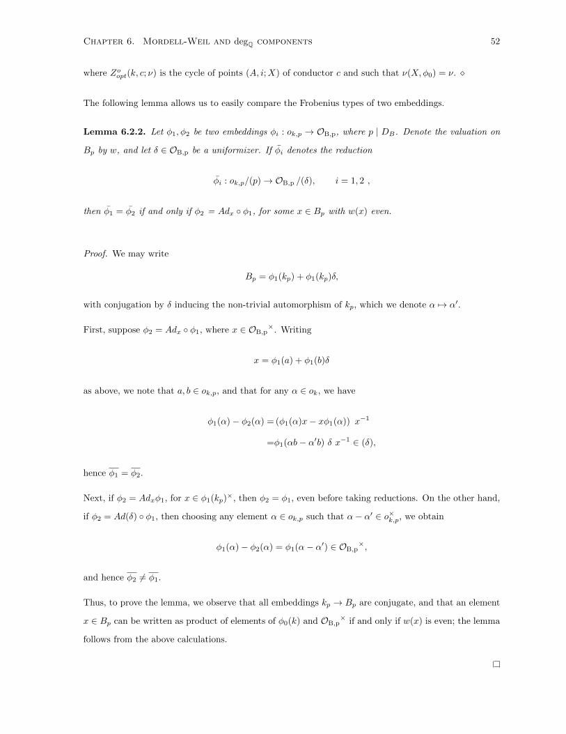
Chapter 6. Mordell-Weil and degQ components 52
where Zoopt(k, c; ν) is the cycle of points (A, i;X) of conductor c and such that ν(X,φ0) = ν.
The following lemma allows us to easily compare the Frobenius types of two embeddings.
Lemma 6.2.2. Let φ1, φ2 be two embeddings φi : ok,p → OB,p, where p | DB. Denote the valuation on
Bp by w, and let δ ∈ OB,p be a uniformizer. If φi denotes the reduction
φi : ok,p/(p)→ OB,p /(δ), i = 1, 2 ,
then φ1 = φ2 if and only if φ2 = Adx φ1, for some x ∈ Bp with w(x) even.
Proof. We may write
Bp = φ1(kp) + φ1(kp)δ,
with conjugation by δ inducing the non-trivial automorphism of kp, which we denote α 7→ α′.
First, suppose φ2 = Adx φ1, where x ∈ OB,p×. Writing
x = φ1(a) + φ1(b)δ
as above, we note that a, b ∈ ok,p, and that for any α ∈ ok, we have
φ1(α)− φ2(α) = (φ1(α)x− xφ1(α)) x−1
=φ1(αb− α′b) δ x−1 ∈ (δ),
hence φ1 = φ2.
Next, if φ2 = Adxφ1, for x ∈ φ1(kp)×, then φ2 = φ1, even before taking reductions. On the other hand,
if φ2 = Ad(δ) φ1, then choosing any element α ∈ ok,p such that α− α′ ∈ o×k,p, we obtain
φ1(α)− φ2(α) = φ1(α− α′) ∈ OB,p×,
and hence φ2 6= φ1.
Thus, to prove the lemma, we observe that all embeddings kp → Bp are conjugate, and that an element
x ∈ Bp can be written as product of elements of φ0(k) and OB,p× if and only if w(x) is even; the lemma
follows from the above calculations.
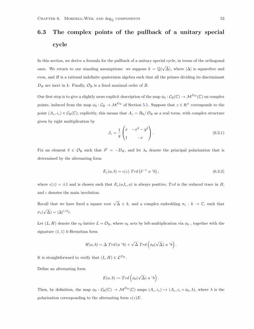
Chapter 6. Mordell-Weil and degQ components 53
6.3 The complex points of the pullback of a unitary special
cycle
In this section, we derive a formula for the pullback of a unitary special cycle, in terms of the orthogonal
ones. We return to our standing assumptions: we suppose k = Q(√
∆), where |∆| is squarefree and
even, and B is a rational indefinite quaternion algebra such that all the primes dividing its discriminant
DB are inert in k. Finally, OB is a fixed maximal order of B.
Our first step is to give a slightly more explicit description of the map φ0 : CB(C)→MDB (C) on complex
points, induced from the map φ0 : CB →MDB of Section 5.1. Suppose that z ∈ H± corresponds to the
point (Az, iz) ∈ CB(C); explicitly, this means that Az = BR/OB as a real torus, with complex structure
given by right multiplication by
Jz =1
y
x −x2 − y2
1 −x
. (6.3.1)
Fix an element δ ∈ OB such that δ2 = −DB , and let λ0 denote the principal polarization that is
determined by the alternating form
Ez(a, b) = ε(z) Trd(δ−1 a ιb
), (6.3.2)
where ε(z) = ±1 and is chosen such that Ez(aJz, a) is always positive, Trd is the reduced trace in B,
and ι denotes the main involution.
Recall that we have fixed a square root√
∆ ∈ k, and a complex embedding σ1 : k → C, such that
σ1(√
∆) = |∆|1/2i.
Let (L,H) denote the ok-lattice L = OB, where ok acts by left-multiplication via φ0 , together with the
signature (1, 1) k-Hermitian form
H(a, b) = ∆ Trd (a ιb) +√
∆ Trd(φ0(√
∆) a ιb).
It is straightforward to verify that (L,H) ∈ LDB .
Define an alternating form
E(a, b) := Trd(φ0(√
∆) a ιb).
Then, by definition, the map φ0 : CB(C) → MDB (C) maps (Az, iz) 7→ (Az, iz φ0, λ), where λ is the
polarization corresponding to the alternating form ε(z)E.

Chapter 6. Mordell-Weil and degQ components 54
Set ΓL = GU(L), the group of unitary similitudes of L. We define D(L)± to be the space of all definite
kR lines in LR. Then we may uniformize the complex points of MDB (C) as the quotient:
MDB (C)L ' [ΓL\D(L)] '[ΓL\D(L)±
],
where MDB (C)L is the connected component of MDB (C) corresponding to L as in (3.3.1).
We can then describe the map φ0 on these spaces explicitly.
Lemma 6.3.1. Let Ik =√
∆⊗ |∆|−1/2 ∈ kR, and let L = Lφ0 . Define a map φ0 : H± → D(L)±, by the
formula
φ0(z) = v ∈ BR | vJz = −φ0(Ik)v ∈ D(L)±.
Then the following diagram commutes:
CB(C) −−−−→φ0
MDB (C)L
'y y'[
O×B \H±]−−−−→
φ0
[Γ\D(L)±
]Proof. First, we check that the bottom map is well-defined: note that if γ ∈ O×B , then Jγ·z = γJzγ
−1.
Thus φ0(γ · z) = φ0(z) · γ, and as right-multiplication by γ evidently defines an element of GU(L), we
are done.
The fact that the diagram commutes then follows directly from the constructions of the respective
complex uniformizations (the vertical arrows).
We now investigate the corresponding diagram for special cycles. Consider a point (Az, ιz) ∈ CB(C),
with Az = BR/OB as a real torus, with the action ιz : OB → End(A) induced by left-multiplication on
BR, and the complex structure is given by right-multiplication by the matrix Jz as in (6.3.1).
Now suppose X : Az → Az is an OB-linear endomorphism. Then X induces an OB-linear endomorphism
OB = H1(Az,Z)→ H1(Az,Z) = OB,
and so, as an endomorphism of BR/OB, the map X is determined by right-multiplication by an element
x = X(1) ∈ OB. Moreover, as X is holomorphic, we have the relation
xJz = Jzx

Chapter 6. Mordell-Weil and degQ components 55
in BR.
In addition,
X2 = t2∆ ⇐⇒ x2 = t2∆,
and so from this discussion, we see, for t ∈ Z,multiplicity of (Az, ιz)
in Zo(t2|∆|)
= #x ∈ OB | Trd(x) = 0, x2 = t2∆, Jzx = xJz
. (6.3.3)
We note, however, that the right hand side of this equation is always either 0 or 2. Indeed, if Jz and x
commute, then by Lemma 6.1.1 (applied to BR instead of B), we must have x = ± t|∆|1/2Jz. If we set
xz := t|∆|1/2Jz, (6.3.4)
then whenever the right hand side of (6.3.3) is non-empty, it consists of the two elements xz,−xz.
Our next task is to carry out a similar analysis for the unitary special cycles. Fix a fractional ideal a in
k, and let
Ea = C /σ1(a),
where σ1 : k → C is our fixed complex embedding. There is a natural ok-action of signature (1, 0), given
by restricting the embedding σ1 to ok, and also a natural principal polarization, defined as in (3.3.2),
which together define a point E+a ∈ E+(C) - c.f. the discussion preceding Lemma 3.3.2.
If we view the point (Az, ιz) ∈ CB(C) as a CM abelian surface via the fixed optimal embedding φ0 :
ok → OB, then any ok-linear map ξ : Ea → Az is determined by the map on homology
ξ : a = H1(Ea,Z)→ H1(Az,Z) = OB .
Let
ξ :=1
N(a)ξ(N(a)) ∈ φ0(a)−1OB .
By assumption, we have that the complex structure on Ea is given by multiplication by σ1(√
∆⊗|∆|−1/2).
Hence, in BR = Lie(Az), we have the relations
ξJz = ξ(σ1(|∆|−1/2 ⊗√
∆)) by holomorphicity of ξ
= |∆|−1/2φ0(√
∆)ξ by ok − linearity of ξ,
which in turn is equivalent to the relation
Jz = |∆|−1/2 ξ−1φ0(√
∆)ξ. (6.3.5)

Chapter 6. Mordell-Weil and degQ components 56
Conversely, any element ξ ∈ φ0(a)−1OB satisfying (6.3.5) defines an ok-linear morphism ξ : Ea → Az.
By Lemma 3.3.2 and the discussion preceding Lemma 6.3.1, we have
qEa,Az (ξ) = ε(z)Nrd(ξ)N(a)∆,
where ε(z) = ±1 is determined in (6.3.2).
Note that every complex point in E+(C) is isomorphic to a curve E+a constructed as above, and the
isomorphism classes are parametrized by the ideal class group of k.
Summarizing this discussion, we findmultiplicity of (Az, ιz)
in φ∗0Z+(m)
= #∐
[a]∈Cl(k)
ξ ∈ φ0(a)−1OB | Nrd(ξ) = ε(z)m/N(a)∆,
and Jz = |∆|−1/2 ξ−1φ0(√
∆)ξ. (6.3.6)
By a similar argument, we findmultiplicity of (Az, ιz)
in φ∗0Z−(m)
= #∐
[a]∈Cl(k)
ξ ∈ φ0(a)−1OB | Nrd(ξ) = −ε(z)m/N(a)∆,
and Jz = −|∆|−1/2 ξ−1φ0(√
∆)ξ. (6.3.7)
Next, we compare the supports of the orthogonal and unitary cycles.
Suppose we have an ok-linear morphism ξ : E±a → Az, for some point (Az, ιz) ∈ CB(C), which corresponds
as above to the element ξ ∈ φ0(a)−1OB.
Let
x := c · ξ−1φ0(√
∆)ξ,
where c is the conductor of the embedding
hξ := Adξ−1 φ0.
Then x ∈ OB, Trd(x) = 0, x2 = c2∆, and Jzx = xJz. Therefore, right-multiplication by x defines an
OB-linear endomorphism X : Az → Az, and so Az lies in the support of Zoopt(k, c).
Note moreover that if Nrd(ξ) = ±m/N(a)∆, then (as is easily verified locally)
m · ξ−1φ0(√
∆)ξ ∈ OB,
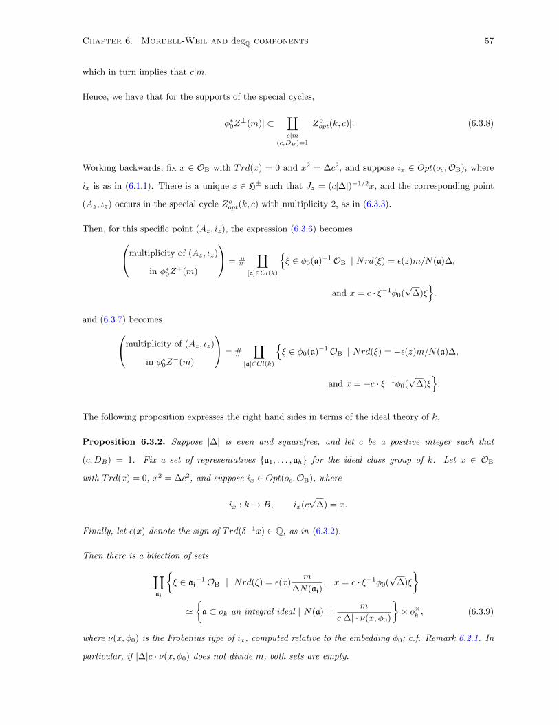
Chapter 6. Mordell-Weil and degQ components 57
which in turn implies that c|m.
Hence, we have that for the supports of the special cycles,
|φ∗0Z±(m)| ⊂∐c|m
(c,DB)=1
|Zoopt(k, c)|. (6.3.8)
Working backwards, fix x ∈ OB with Trd(x) = 0 and x2 = ∆c2, and suppose ix ∈ Opt(oc,OB), where
ix is as in (6.1.1). There is a unique z ∈ H± such that Jz = (c|∆|)−1/2x, and the corresponding point
(Az, ιz) occurs in the special cycle Zoopt(k, c) with multiplicity 2, as in (6.3.3).
Then, for this specific point (Az, iz), the expression (6.3.6) becomesmultiplicity of (Az, ιz)
in φ∗0Z+(m)
= #∐
[a]∈Cl(k)
ξ ∈ φ0(a)−1OB | Nrd(ξ) = ε(z)m/N(a)∆,
and x = c · ξ−1φ0(√
∆)ξ.
and (6.3.7) becomesmultiplicity of (Az, ιz)
in φ∗0Z−(m)
= #∐
[a]∈Cl(k)
ξ ∈ φ0(a)−1OB | Nrd(ξ) = −ε(z)m/N(a)∆,
and x = −c · ξ−1φ0(√
∆)ξ.
The following proposition expresses the right hand sides in terms of the ideal theory of k.
Proposition 6.3.2. Suppose |∆| is even and squarefree, and let c be a positive integer such that
(c,DB) = 1. Fix a set of representatives a1, . . . , ah for the ideal class group of k. Let x ∈ OB
with Trd(x) = 0, x2 = ∆c2, and suppose ix ∈ Opt(oc,OB), where
ix : k → B, ix(c√
∆) = x.
Finally, let ε(x) denote the sign of Trd(δ−1x) ∈ Q, as in (6.3.2).
Then there is a bijection of sets
∐ai
ξ ∈ ai
−1OB | Nrd(ξ) = ε(x)m
∆N(ai), x = c · ξ−1φ0(
√∆)ξ
'a ⊂ ok an integral ideal | N(a) =
m
c|∆| · ν(x, φ0)
× o×k , (6.3.9)
where ν(x, φ0) is the Frobenius type of ix, computed relative to the embedding φ0; c.f. Remark 6.2.1. In
particular, if |∆|c · ν(x, φ0) does not divide m, both sets are empty.

Chapter 6. Mordell-Weil and degQ components 58
Similarly, we have
∐ai
ξ ∈ ai
−1OB | Nrd(ξ) = −ε(x)m
∆N(ai), x = −c · ξ−1φ0(
√∆)ξ
'a ⊂ ok an integral ideal | N(a) =
m
c|∆| · ν(x, φ0)
× o×k . (6.3.10)
Proof. By Noether-Skolem, there exists an element ξ0 ∈ B× such that
hξ0(c√
∆) := c · ξ−10 φ0(
√∆)ξ0 = x. (6.3.11)
Let ξ ∈ B×. By Lemma 6.1.1, we have that hξ = hξ0 if and only if ξ = φ0(a)ξ0 for some a ∈ k×. Thus
∐ai
ξ ∈ ai
−1OB | n(ξ) = ε(x)m
∆N(ai), hξ = ix
(6.3.12)
=∐ai
a ∈ k× | φ0(a) ∈ a−1
i OB ξ−10 , n(a) = ε(x)
m
∆N(ai)Nrd(ξ0)
(6.3.13)
=
a ∈ Ik | φ0(a) ⊂ OB ξ
−10 , N(a) = ε(x)
m
∆Nrd(ξ0)
× o×k , (6.3.14)
where Ik is the group of fractional ideals of k; the equality between the second and third lines follows
from the decomposition Ik = ai × k×.
We first observe that
ε(x) = −sgn(Nrd(ξ0)) = − Nrd(ξ0)
|Nrd(ξ0)|.
This can be seen by noting that for any a, b, we have ε(b−1ab) = sgn(Nrd(b)) · ε(a). Furthermore, if
x0 = φ0(√
∆), ξ0 = 1, then ε(x0) = −1; on the other hand by Noether-Skolem, all x’s satisfying the
hypotheses of the proposition are conjugate to x0, and hence we are done.
Now, by Theorem 6.1.3, we have that the order Oξ0 := ξ0OB ξ−10 and the order O(c) constructed in
Lemma 6.1.2, are conjugate by a finite idele of k. In particular, for every prime p, we may write
ξ0 = ap w(c)p νp ∈ Bp,
for some ap ∈ φ0(k×p ) and νp ∈ NB×p (OB,p); here w(c)p is as in the proof of Lemma 6.1.2. Note that for
p - DB , νp ∈ O×B,p. Suppose p | DB and p is ramified in k. In this case, w(c)p = 1, and, by changing ap
if neccessary, we may also take νp to be a unit, as a uniformizer for kp is a uniformizer for Bp. If p | DB
and p is inert in k, we may similarly choose νp so that ordp(νp) is 0 or 1; note that as in Remark 6.2.1,
we have ∏p|DinB
pordp(νp) = ν(x, φ0).

Chapter 6. Mordell-Weil and degQ components 59
Let a0 be the fractional ideal corresponding to the idele (ap). Replacing a by a a−10 in (6.3.14), translating
the condition φ0(a) ⊂ OB ξ−10 to a collection of local ones, and applying the relation
ε(x)/n(ξ0) = −1/|n(ξ0)|,
it follows that the set in (6.3.14) is the same asa ∈ Ik | φ0(a)p ⊂ OB,pνp−1w(c)−1
p for all p, N(a) =m
|∆| c ν(x, φ0)
. (6.3.15)
We now claim that
φ0(a)p ⊂ OB,pνp−1w(c)−1p for all p ⇐⇒ a ⊂ ok,
which will conclude the proof of (6.3.9) in the statement of the proposition.
For primes p - DB , we have νp ∈ O×B,p, and via an isomorphism chosen as in Lemma 6.1.2,
OB,pw(c)−1p =
p−ra b
p−rc d
| a, b, c, d ∈ Zp
. (6.3.16)
As in Lemma 6.1.2, an element x = α+β√
∆ ∈ kp, with α, β ∈ Qp, is mapped to the matrix
α β
γβ α
,
where ordp(γ) = ordp(|∆|). It is evident from this description that if φ0(x) ∈ OB,pw(c)−1p , then φ0(x) ∈
OB,p.
For primes p|DB , p inert in k, and for which νp /∈ O×B,p, we arrive at the same conclusion, as kp contains
no elements of norm p.
Hence, we conclude that φ0(a) ⊂ OB,p for all p, and as φ0 is an optimal embedding from ok to OB, this
holds if and only if a ⊂ ok.
The proof of (6.3.10) follows in exactly the same way.
As a consequence of these formulas, we obtain the following Shimura lift formulas for the degQ and MW
components:
Theorem 6.3.3. Suppose |∆| is even and squarefree, and (|∆|, 4DB) = 1. Let χk and χ′ be as in Section
5.2 (with d = DB in the notation of that section), and let Opt denote the set of equivalence classes of
optimal embeddings from ok into OB, taken up to O×B -conjugacy.
Recall that the complex points of our stacks and cycles are denoted by Roman letters, so CB = CB(C),
Zo(t) = Zo(t)(C), etc.

Chapter 6. Mordell-Weil and degQ components 60
(i) For any m > 0, we have the following equalities of cycles on CB:
1
h(k)|o×k |∑
[φi]∈Opt
φ∗iZ(m) =
0, if |∆| does not divide m,∑a|m′ χ
′(a) Zo(
(m′)2
a2 |∆|)
if m = |∆|m′.
(ii) Let
Φ∗deg(w) =1
h(k)|o×k |∑m≥0
∑[φi]
degQ φ∗iZ(m) qmw
denote the rational degree of the pullback unitary generating series (c.f. Definition 5.2.4).
Then Sh|∆|
(Φodeg
)(w) = Φ∗deg(w).
(iii) Let
Φ∗MW (w) =1
h(k)|o×k |∑m≥0
∑[φi]
MW (φ∗iZ(m, η)) qmw ,
where MW is the projection onto the MW -component of CH1(CB)R, c.f. (2.2.1).
Then Sh|∆|(ΦoMW ) = Φ∗MW .
Proof. (i) Fixing one embedding φ0 : ok → OB for the moment, we note that Proposition 6.3.2 implies
that
φ∗0Z(m) = |o×k |∑c|m
(c,DB)=1
∑ν|DB
ρ
(m
|∆|cν
)Zoopt(k, c, ν), (6.3.17)
where Zoopt(k, c, ν) denotes the cycle of special endomorphisms occurring in the support of Zo(|∆|m2)
of conductor c and Frobenius type ν(X,φ0) = ν, and ρ(N) denotes the number of integral ok-ideals of
norm N .
For a fixed m with |∆| dividing m, and fixed embedding φ0, there is exactly one value of ν for which
ρ(m/|∆|cν) is non-zero; namely the unique squarefree integer ν(m) dividing (m,DB) such that
ordp(ν(m)) ≡ ordp(m) modulo 2, for all p|DB .
Therefore, we have
φ∗0Z(m) = |o×k |∑c|m
(c,DB)=1
ρ
(m
|∆|c ν(m)
)Zoopt(k, c, ν(m)). (6.3.18)
On the other hand, as N(OB)/O×B acts transitively on the set of Frobenius types, there are h(k) em-

Chapter 6. Mordell-Weil and degQ components 61
beddings of each type. Hence
1
h(k)|o×k |∑[φi]
φ∗iZ(m) =∑c|m
(c,DB)=1
ρ
(m
|∆|c ν(m)
)Z0opt(k, c)
=∑c|m∗
(c,DB)=1
ρ
(m∗
c
)Z0opt(k, c), (6.3.19)
where m∗ = m/|∆| ν(m); we follow the convention here that if |∆| does not divide m, the sum on the
right hand side is empty.
We claim that for any T > 0, we have ∑a|T
χk(a) = ρ(T ).
Postponing the proof of this claim temporarily, it follows that if ordp(T ) is even for all p|DB , we then
have ∑a|T
χ′(a) = ρ(T )
as well; recall that χ′ is the character obtained by inducing χk to 4DB |∆|.
Putting this into (6.3.19), and setting m′ = m/|∆|, we obtain
1
h(k)|o×k |∑[φi]
φ∗iZ(m) =∑c|m∗
(c,DB)=1
∑a|m∗/c
χ′(a) Zoopt(k, c)
=∑a|m∗
χ′(a)∑c|m′/a
(c,DB)=1
Zoopt(k, c)
=∑a|m′
χ′(a) Zo(|∆| (m
′)2
a2
). (6.3.20)
As the right hand side is 0 when |∆| does not divide m, by convention, this proves the desired relation.
(ii) As Φodeg is a holomorphic modular form, it suffices to check that the relations (4.2) and (4.3) hold
at the level of Fourier coefficients; in the notation of that section, we have N = DB , t = |∆|, κ = 3 and
λ = 1. In other words, let
B(m) :=∑a|m
χ′(a) degQ Zo
(|∆|m
2
a2
), for m > 0.
Note that the character χ′ is the one denoted χt in (4.2), for our particular case.
We also set
B(0) :=−i2π
L(1, χ′) degQ Zo(0) =
i
2πL(1, χ′) degQ ω
0Q,

Chapter 6. Mordell-Weil and degQ components 62
where χ′ is the Gauss sum
χ′(a) =
4DB |∆|∑h=1
χ′(h)e2πiah/4DB |∆|.
We then need to show that the m’th Fourier coefficient of Φ∗deg is equal to B(m/|∆|).
For m > 0, the desired claim follows from applying the functional degQ to both sides of (6.3.20), which
yields
1
h(k)|o×k |∑[φi]
degQ φ∗iZ(m) = B(m′) = B
(m
|∆|
)as required.
Turning now to the constant term, first note that by Lemma 5.1.1, we have degQ φ∗iω = degQ ω
o for all
i. Also, recall that if o(DB) denotes the number of prime factors in DB , which by assumption are all
inert in k, we have
#Opt = h(k)2o(DB).
These facts taken together, along with the definition of the constant term (5.2.2), yields
1
h(k)|o×k |∑[φi]
degQ φ∗i Z(0)Q =
i
2πL(1, χ′) degQ ω
o = B(0)
as required.
(iii) As ΦoMW is holomorphic, it suffices to verify the equations (4.2) and (4.2) for the Fourier coefficients
of the Shimura lift hold, with Φ∗MW playing the role of G|∆| there.
Recall that the restriction to the generic fibre is an isomorphism
resQ : MW∼−→ MW,
where MW = Jac(CB)(Q)⊗ R, the Mordell-Weil space of CB.
In particular, for any arithmetic cycle Z = (Z, gZ) ∈ CH1(CB)R, we have
resQMW (Z) = resQ
(Z −
degQZdegQ ω
0ω0
)= ZQ−
degQ(ZQ)
degQ ω0
ω0Q,
In light of this, we note that the constant terms of ΦoMW and Φ∗MW both vanish, while the identity for
the non-constant Fourier coefficients follows directly from (6.3.20).
It remains to provide the proof of the following lemma:

Chapter 6. Mordell-Weil and degQ components 63
Lemma 6.3.4. For any integer T > 0,
∑a|T
χk(a) = ρ(T ).
Proof. Both sides are multiplicative in T , so it suffices to prove the formula for T = pn. If p is split, we
have χk(p) = 1, and hence
ρ (pn) = n+ 1 =∑a|pn
χk(a).
The cases for p ramified or inert are handled identically.

Chapter 7
Analytic components
In this section, we compute the Shimura lifts of the “analytic” components of the orthogonal generating
series Φo(τ). Recall that these components are defined as follows. Define C∞(CB(C))0 to be the space
of real-valued smooth functions f that are orthogonal to the Hodge class - i.e∫CB(C)
f · c1(ωo) = 0,
where c1(ωo) denotes the first Chern form of the Hodge class, as in Section 2.5. For such a function f ,
we obtain a class
a(f) := (0, f) ∈ CH1(CB)R.
Let Z = (Z, g) ∈ CH1(CB)R, so that
ddcg + δZ(C) = [ωZ ]
for some smooth (1,1) form ωZ on CB(C). Then the height pairing between Z and the element a(f) as
above is given by
〈Z, a(f)〉 =
∫CB(C)
f · ωZ .
In particular, for the orthogonal special cycles Zo(n, v) = (Zo(n), Gro(n, v)) with n 6= 0, we have that
ddc[Gro(n, v)] + δZo(n) = [ψo(n, v)dµ],
where
ψo(n, v)(z) =1
2π
∑x∈OB
0(n)
(4πv Ro(x, z) + 2q(x) − 1) e−2πvRo(x,z)
64

Chapter 7. Analytic components 65
and dµ = dx · dy/y2 is the usual hyperbolic measure on H±. Recall that for z ∈ H±, we define
Ro(x, z) := −2Nrd(xz),
where xz denotes the orthogonal projection of x onto the (negative-definite) plane J⊥z , with respect to
Nrd, the reduced norm on B(R); see Section 2.4.
Furthermore, 〈Zo(0, v), a(f)〉 = 0, as f is orthogonal to the Hodge class by assumption. Hence, the
analytic components of the generating series Φo(τ) are given by the expressions
Φof (τ) := 〈Φo(τ), a(f)〉 =∑n∈Zn 6=0
(∫CB(C)
ψo(n, v)(z)f(z)dµ(z)
)exp(2πinτ).
As explained in [17, §4.4], this generating series can be identified as the Fourier expansion of a certain
theta integral of f . In particular, when f is a Maass form on CB(C), then Φo(f) is a non-holomorphic
Maass form for Γ0(4(DB)0) of weight 3/2, c.f. [17, Corollary 4.4.2].
Theorem 7.1. Let f ∈ C∞(CB(C))0. Then
Sh|∆|(Φof)
(w) = 〈Φ∗(w), a(f)〉,
as Fourier expansions at ∞.
Proof. We begin by computing the pullbacks of the hyperbolic measure appearing in the Green’s equation
for the unitary special cycles.
Let φ : ok → OB be an optimal embedding. Recall that morphism φ : CB(C)→MDB (C) induced by φ
on complex points is equivalent to the map
φ : H± → D(BR), z 7→v ∈ BR, vJz = −|∆|−1/2φ(
√∆)v
,
where we view B as an k module by left-multiplication via φ, and D(BR) denotes the space of negative-
definite kR-lines in BR - see Lemma 6.3.1.
We may describe this map even more explicitly, by specifying a particular base point in D(BR) . Recall
that we have fixed an isomorphism BR 'M2(R). Without loss of generality, we may assume that under
this isomorphism, |∆|−1/2φ(√
∆) corresponds to
−1
1
.
Write
B = φ(k) +B−,
Chapter 7. Analytic components 66
where B− is the orthogonal complement to φ(k), under the quadratic form determined by Q(x) =
(|∆|/2)Nrd(x), a rational multiple of the reduced norm of B; under our present assumptions, B− is
exactly the set of symmetric traceless matrices. If we set
e =1
|∆|1/2
1
1
, f =1
|∆|1/2
1
−1
,
then e, f form a standard basis for BR over kR; i.e (e, e) = −(f, f) = 1, (e, f) = 0. This allows us to
define a complex coordinate on D(BR) via the map
ζ 7→ Z(ζ) = spankR (ζe+ f) , ζ ∈ U1 := open unit disc in C,
which induces an identification D(BR) ' U1.
For β ∈ BR, η ∈ R>0, a a fractional ideal of k, and Z ∈ D(BR), define functions
ψu+(β, a, η)(Z) =1
2π[4πN(a)η (R(β,Z) + 2Q(β))− 1] e4πN(a)Rη
and
ψu−(β, a, η)(Z) =1
2π[4πN(a)ηR(β,Z)− 1] e4πN(a)(R+2Q)η,
where
R = R(β,Z) := −2Q(βZ), βZ := orthogonal projection of β onto Z.
Recall that for unitary special cycles Z(`), ` 6= 0 (c.f. §3.5), we had defined Green’s functions Gr(`, η)
satisfying
ddc[Gr(`, η)] + δZ(`) = [ψu(`, η)dω(ζ)],
where, with respect to the ζ-coordinate described above,
dω(ζ) = idζ ∧ dζ
(1− |ζ|2)2,
and
ψu(`, η)(ζ) =∑[a]
∑β∈a−1OB
2Q(β)=`/N(a)
ψu+(β, a, η)(ζ) +∑
β∈a−1OB
2Q(β)=−`/N(a)
ψu−(β, a, η)(ζ)
.
It is then a direct computation to show that with respect to this coordinate system, for z = x+ iy ∈ H,
we have φ(z) = z−iz+i ∈ U
1, and hence
φ∗(idζ ∧ dζ
(1− |ζ|2)2
)=
1
2
idz ∧ dz2y2
. (7.1)
Chapter 7. Analytic components 67
Define
Θo(τ, z) :=∑n∈Zn 6=0
ψo(n, v)(z) qnτ
and
Θ∗(w, z) :=1
h(k)|o×k |∑[φi]
∑`∈Z6=0
1
2ψu(`, η)(φi(z))q
`w;
noting that CB(C) is compact, we then have
〈Φo(τ), a(f)〉 =
∫CB(C)
Θo(τ, z)f(z)dµ(z), 〈Φ∗(w), a(f)〉 =
∫CB(C)
Θ∗(τ, z)f(z)dµ(z),
and so to prove the theorem, it suffices to prove the following relation:
Sh|∆| (Θo(·, z)) (w)
?= Θ∗(w, z). (7.2)
We begin by computing the left hand side, using the Poincare series expansion for Niwa’s theta kernel
from Proposition 4.4 - in our present case, κ = 3, λ = 1, N = DB , t = |∆|, and χ′ = 14DB · χk. Upon
unfolding the integral, we obtain
Sh|∆| (Θo(·, z)) (w) = C(λ)
∫Γ0(4N |∆|)\H
v3/2 Θo(|∆|τ, z) Θ#Niwa(τ, w) dµ(τ)
=1
8
∫Γ∞\H
v3/2 Θo(|∆|τ, z)
[∑m∈Z
χ′(m)
1∑µ=0
4µ(ηmv
)1−µ
× exp
(−πη
2m2
4v
)θµ(τ,−ξm/2)
]dµ(τ),
where
θµ(τ,−ξm/2) =∑`∈Z
`µe(τ`2 − ξ`m
)for µ = 0, 1.
Substituting in this latter expression, together with the Fourier expansion
Θo(|∆|τ, z) =∑n
ψo(n, |∆|v)(z) e(|∆|nτ),
it is clear that only terms in which |∆|n = `2 contribute. In this case, as |∆| is squarefree, this implies
that |∆| | `, and hence we obtain contributions only when n is of the form |∆|r2. The integral then

Chapter 7. Analytic components 68
becomes
Sh|∆| (Θo) (w) =
1
8
∑m,r∈Z
χt(m)
∫ ∞0
v3/2ψo(|∆|r2, |∆|v)(z)
×
[1∑
µ=0
4µ(ηmv
)1−µ(|∆|r)µ
]exp
(−4π|∆|2r2v − πη2m2
4v
)dv
v2
× exp(2πi|∆|mrξ)
=1
4
∑`∈Z6=0
∑m||`|
χ′(m)∑x∈OB
x2=∆(`2/m2)
I(m, `, x)(z) exp(2πi|∆|`ξ),
where
I(m, `, x)(z) :=1
2π
∫ ∞0
v3/2 (4π|∆|v Ro(x, z) + 2Nrd(x) − 1)
×
[1∑
µ=0
4µ(ηmv
)1−µ(|∆|`m
)µ]
× exp
(−2π 2Nrd(x) +Ro(x, z) |∆|v − πη2m2
4v
)dv
v2.
This integral is a sum of Bessel K-functions with half-integral argument, which may be evaluated ex-
plicitly; see formula (8.468) of [6]. In particular for a, b > 0, we have the formulae:∫ ∞0
v−3/2e−π2 (av+b/v)dv =
√2
be−π√ab (7.3)∫ ∞
0
v−1/2e−π2 (av+b/v)dv =
√2
ae−π√ab (7.4)∫ ∞
0
v1/2e−π2 (av+b/v)dv =
√2(1 + π
√ab)
πa3/2e−π√ab. (7.5)
After applying these formulæ, we arrive at the expression
I(m, `, x)(z) =1
π
(πηm
(√2|∆| Ro(x, z) + 2Nrd(x)1/2 + 2|∆| `
m
)− 1
)× exp
(−√
2|∆|πm Ro(x, z) + 2Nrd(x)1/2 η).
The key step in the proof is the following lemma, which relates the orthogonal majorants on OB with
the unitary majorants induced from an embedding φ0 : ok → OB.
Lemma 7.2. Let φ0 : ok → OB be an embedding, and x ∈ OB with x2 = (`2/m2)∆. By Noether-Skolem,
we may write
x =`
mβ−1 φ0(
√∆) β,

Chapter 7. Analytic components 69
for some β ∈ B×. Let z ∈ H±, and suppose that φ0(z) ∈ D(Bφ0). Then
Ro(x, z) + 2Nrd(x) =2`2|∆|m2Q(β)2
(R(β, φ0(z)) +Q(β))2,
where Q(β) = (|∆|/2)Nrd(β).
Postponing the proof of this lemma, we note that without loss of generality, we may assume that φi(z)
is a negative plane, for all i; if not, we may replace φi with its image under conjugation by an element
of O×B with norm −1.
Suppose x and β are related as in the lemma; if 2Q(β) = +|∆|`/N(a), then
I(m, `, x) =1
π[(4πN(a)η(R(β, φ0(z)) + 2Q(β))− 1] e−4πN(a)(R+Q)η
= 2 ψ+(β,N(a), η) (φ0(z)) e−4πN(a)Q(β)η
and if instead 2Q(β) = −|∆|`/N(ai), then
I(m, `, x) =1
π[4πN(a)η(R(β, φ0(z))− 1] e−4πN(a)(R+Q)η
= 2 ψ−(β,N(a), η) (φ0(z)) e4πN(a)Q(β)η;
note in particular the quantity I(m, `, x) = I(`, x) is independent of m.
Fix ` , and x as above, and let c be the conductor of ix. As a direct consequence of Proposition 6.3.2,
we may compute the number of β’s of the appropriate norm that satisfy the hypotheses of the lemma
above:
#∐[φ]
∐[a]
β ∈ a−1OB | 2Q(β) = ±|∆|`/N(a), Adβ−1 φ = ix
= h(k) |o×k | ρ
(|`|∗
c
),
where ρ(T ) is the number of integral ideals in ok of norm T , and |`|∗ is any integer dividing |`| such that
ordp|`|∗ ≡ 0 modulo 2, for all p|DB
c.f. equation (6.3.19).

Chapter 7. Analytic components 70
Then
Sh|∆|(Θo)(w, z) =
1
4
∑`∈Z` 6=0
∑m||`|
χ′(m)∑x∈OB
x2=∆(`2/m2)
I(`, x)(z) exp(2πi|∆|`ξ)
=∑`∈Z` 6=0
∑c||`|
(c,DB)=1
1
4
∑x∈OB
Q(x)'kix∈Opt(oc,OB)
∑m||`|/c
χ′(m)
I(`, x)(z) exp(2πi|∆|`ξ)
=∑`∈Z6=0
∑c||`|
(c,DB)=1
1
4
∑x∈OB
Q(x)'kix∈Opt(oc,OB)
ρ
(|`|∗
c
)I(`, x)(z) exp(2πi|∆|`ξ);
here we have used the fact ∑m|c−1|`|
χ′(m) =∑
m|c−1|`|∗χ′(m) = ρ(|`|∗/c),
c.f. the proof of Theorem 6.3.3.
Thus, replacing the sum on x’s with sums on β’s, we obtain
Sh|∆|(Θo)(w, z) =
1
2h(k)|o×k |∑[φ]
∑`∈Z` 6=0
∑[a]
∑c||`|
(c,DB)=1
×
( ∑β∈a−1OB
2Q(β)=|∆|`/N(a)c(β,φ)=c
ψu+(β,N(a), η) (φ(z))
+∑
β∈a−1OB
2Q(β)=−|∆|`/N(a)c(β,φ)=c
ψu−(β,N(a), η) (φ(z))
)× exp(2πi|∆|`w)
=1
2h(k)|o×k |∑[φ]
∑`∈Z` 6=0
∑[a]
( ∑β∈a−1OB
2Q(β)=|∆|`/N(a)
ψu+(β,N(a), η) (φ(z))
+∑
β∈a−1OB
2Q(β)=−|∆|`/N(a)
ψu−(β,N(a), η) (φ(z))
)exp(2πi|∆|`w).
Since Q(OB) ⊂ |∆|2 Z, we may continue the equality:
=1
2h(k)|ok|×∑[φ]
∑`∈Z` 6=0
∑[a]
( ∑β∈a−1OB
2Q(β)=`/N(a)
ψu+(β,N(a), η) (φ(z))
+∑
β∈a−1OB
2Q(β)=−`/N(a)
ψu−(β,N(a), η) (φ(z))
)exp(2πi`w);
As this final expression is precisely Θ∗(w, z), we are done.

Chapter 7. Analytic components 71
Proof of Lemma 7.2. We first show the conclusion of the lemma holds for a specific z ∈ H, and then
demonstrate that it holds for all z by the appealing to the invariance properties of the majorants.
Using the given embedding φ0 : k → B, we may write B = φ0(k) + θφ0(k), for some θ ∈ B×, with
θ2 ∈ Q>0 and θφ0(a) = φ0(a)θ for all a ∈ k.
Let B− = θφ0(k); note that this is exactly the orthogonal complement to φ0(k) with respect to the form
Q(β) = (|∆|/2)Nrd(β).
Let z0 ∈ H be such that Jz0 = |∆|−1/2φ0(√
∆), under our fixed isomorphism BR ' M2(R). It follows
immediately that φ0(z0) = B−R , a negative definite kR-line. In addition, B−R is a negative definite R-plane
in B0R, the trace-0 elements of BR, and the point in Do(B0
R) corresponding to z0 (ignoring orientations)
is again B−R , c.f. §2.4.
Supposing that
x =`
mβ−1φ0(
√∆)β,
we may write β = φ0(β1) + θφ0(β2), with βi ∈ k ⊗Q R ' C. Then
x =`
Nrd(β)mιβ φ0(
√∆)β
=`
Nrd(β)mφ0(√
∆)(|β1|2 − θ2|β2|2 + 2θβ1β2
),
and hence
Ro(x, z0) + 2Nrd(x) = − 8`2|∆|m2n(β)2
n(θ)|β1|2|β2|2 + 2`2|∆|m2
=2`2|∆|m2Q(β)2
(|∆|2θ2|β1|2|β2|2 +Q(β)2
),
where we write |a|2 = aa, for a ∈ k. On the other hand, we have
R(β, φ0(z0)) = R(β,B−) = |∆|θ2|β2|2, Q(β) =|∆|2
(|β1|2 − θ2|β2|2
),
and one can see directly that
|∆|2θ2|β1|2|β2|2 +Q(β)2 = [R(β, φ0(z0)) +Q(β)]2,
as required. Hence we obtain the conclusion of the lemma in the special case z = z0.
Now suppose that z ∈ H is arbitrary. We may write z = γ · z0, for some γ ∈ SL2(R). Note that this
implies Jz = γJz0γ−1. Since by definition we have φ0(z) = v ∈ BR | vJz = −|∆|−1/2φ0(
√∆)v, it
follows immediately that
φ0(z) = φ0(z0) · γ−1;

Chapter 7. Analytic components 72
note the latter is again a negative kR-stable line.
For the orthogonal majorants, we have
Ro(x, z) = Ro(x, γ · z0) = Ro(γ−1xγ, z0),
while for the unitary majorants, we have
R(βγ, ζ) = R(β, ζγ−1).
Hence, applying the lemma for z = z0 to the vector γ−1xγ, we have
Ro(x, z) + 2Nrd(x) = Ro(γ−1xγ, z0) + 2Nrd(γ−1xγ, z0)
=2`2|∆|
m2Q(βγ)2(R(βγ, φ0(z0)) +Q(βγ))
2
=2`2|∆|m2Q(β)2
(R(β, φ0(z)) +Q(β))2,
since Q(βγ) = Nrd(γ)Q(β) = Q(β); this concludes the proof of the lemma.
Though it is not required for our purposes, we remark that if z ∈ H−, then a similar calculation shows
that
Ro(x, z) + 2Nrd(x) =2`2|∆|m2Q(β)2
(R(β, φ0(z)⊥) +Q(β)
)2.

Chapter 8
Vertical components
8.1 Dieudonne modules and deformations of p-divisible groups
In this section, we briefly recall some of the well-known tools that will be needed in order to describe our
moduli spaces in characteristic p. The remarkable feature of this theory is that it will allow us to think
about some aspects of abelian varieties in characteristic p in terms of linear algebraic data, analogous
to the complex case. References in this section are from the lecture notes [3], which I found to be a
succinct guide to the theory; the inquisitive reader can find references to the original literature therein.
We begin by recalling the definition of a p-divisible group (also referred to as a Barsotti-Tate group at
various points in the literature):
Definition 8.1.1. A p-divisible group of height h over a scheme S is an inductive system (Gv)v≥0
where
• Gv is a finite locally free commutative group scheme over S of order pvh, and
• for each v,
1→ Gv → Gv+1[pv]→ Gv+1
is exact; i.e. Gv is identified with the kernel of multiplication by pv on Gv+1.
For us, the key example of a p-divisible group is the Barsotti-Tate group of an abelian variety A: define
A[pn] = ker[pn : A→ A], and
A[p∞] := (A[pn])n,
73
Chapter 8. Vertical components 74
with forms an inductive system via the natural inclusions A[pn] → A[pn+1]. For reasons that will be
clear shortly, this is precisely the right substitute for the Tate module in characteristic p.
A remarkable fact is that in characterstic p, deformations of an abelian variety are controlled by its
p-divisible group:
Theorem 8.1.2 (Serre-Tate, Thm. 2.7 of [3]). Let S be a scheme on which p is locally nilpotent, and S0
a closed subscheme defined by a locally nilpotent sheaf of ideals. Let AVS denote the category of abelian
schemes over S, and Def(S, S0) denote the category whose objects are tuples (A0, X, ρ), where
• A0 is an abelian scheme over S0,
• X is a p-divisible group over S,
• and ρ : X ×S S0 → A0[p∞] is an isomorphism of p-divisible groups.
A morphism (A0, X, ρ) → (A′0, X′, ρ′) in Def(S, S0) consists of a pair of maps f : A0 → A′0 and
g : X → X ′ of abelian schemes and p-divisible groups respectively, such that ρ′ gS0= ρ f [p∞].
Then the natural map
AVS → Def(S, S0), A 7→ (A×S S0, A[p∞], ρnat)
is an equivalence of categories; here ρnat is the natural identification A[p∞]× S0 ' (A× S0)[p∞].
An immediate corollary is that if we fix an abelian variety A0/S0, then the category of deformations of
A0 is equivalent to the category of deformations of A0[p∞].
We now study p-divisible groups over a perfect field K of characteristic p. Let W(K) denote the ring of
Witt vectors, and note that W(K) comes equipped with an endomorphism σ : W(K) → W(K) lifting
the action of the Frobenius endomorphism of K.
We define a Dieudonne module over K to be a triple (M,F, V ), consisting of a free finite-rank W(K)-
module M , together with a pair of endomorphisms F, V : M →M such that
• F is σ-linear, i.e. F (a ·m) = σ(a) · F (m) for all a ∈W(K),m ∈M ;
• V is σ−1- linear, and
• F V = V F = p.

Chapter 8. Vertical components 75
The following theorem asserts that one can classify p-divisible groups over K in terms of such modules:
Theorem 8.1.3 (c.f. Thm 4.33, [3]). (i) There is a (covariant) equivalence between the category of p-
divisible groups over K and the category of Dieudonne modules over K. Moreover, this equivalence
is exact.
(ii) If X is a p-divisible group with corresponding Dieudonne module M(X), and Serre dual X∨, then
there is a canonical identification
M(X∨) ' HomW(K)(M(X),W(K));
the right hand side is a Dieudonne module with operators F∨ and V ∨ defined by
(F∨ · φ)(m) = (σ φ)(V m), (V ∨ · φ)(m) = (σ−1 φ)(Fm),
for all φ ∈ Hom(M(X),W(K)) and m ∈M(X).
It is worth pointing out that one can explicitly realize this equivalence of categories (e.g. [3, §4]); however
for our present purposes, we shall content ourselves to view it as a black box.
Finally, we indicate how the deformation theory of a p-divisible group X0 over K is controlled by its
Dieudonne module; this is the content of Grothendieck-Messing theory, and is the main technical tool
we require to formulate our results on moduli spaces of abelian surfaces in characteristic p.
Theorem 8.1.4 (Grothendieck-Messing, c.f. [3], Theorem 2.4). Let X0 be a p-divisible group over
a commutative ring R0. Then there exists a functor D(X0/·) which associates to any nilpotent PD-
extension R of R01 a free R-module D(X0/R) of rank h = height(X0). This functor satisfies the
following properties:
(i) Suppose X/R is a p-divisible group lifting X0, with Serre dual X∨. Then there is a canonical exact
sequence
0→ Lie(X∨)∨ → D(X0/R)→ Lie(X)→ 0,
where Lie(X∨)∨ is the R-linear dual of Lie(X∨), and such that D(X0/R)⊗R R0 = D(X0/R0).
1A nilpotent PD extension is a surjective map R → R0 with nilpotent kernel, together with a PD structure, c.f.Definition 2.2 of [3]; the PD structure is what allows one to make sense of exponentials and logarithms in positivecharacteristic. If the kernel of the map R → R0 is generated by p, as is the case when R is the ring of the Witt vectorsW (F) and R0 = F, then there is a canonical PD structure.

Chapter 8. Vertical components 76
(ii) If X = A[p∞] is the Barsotti-Tate group of an abelian variety over R, and is a deformation of X0,
then there is a canonical identification of the exact sequence in (i) with the Hodge filtration:
0→ Fil1(H1dR(A))→ H1
dR(A)→ Lie(A)→ 0.
(iii) There is an equivalence between the categoryR− direct summands F ⊂ D(X0/R)
with
F ⊗R0 = Lie(X∨0 )∨ ⊂ D(X0/R0) = D(X0/R0)⊗K
and the category of deformations of X0 to R, functorially in R.
(iv) Let f : X0 → Y0 denote a morphism of p-divisible groups over R0. For a nilpotent PD-extension
R → R0, we obtain a map D(f/R) : D(X0/R)→ D(Y0/R). Suppose X and Y are lifts of X0 and
Y0 to R, corresponding to the direct summands FX ,FY in D(X0/R) and D(Y0/R) respectively.
Then f lifts to a morphism f : X → Y over R if and only if
D(f/R) (FX) ⊂ FY .
(v) Suppose R0 = K is a perfect field of characteristic 0, and X0 a p-divisible group over K. Let M =
M(X0) denote the Dieudonne module of X0. Then for any W(K)-algebra R equipped with a PD-
structure R→ K compatible with the canonical PD structure on W(K), we have an identification
M ⊗W(K) R ' D(X0/R).
Moreover, for R = W(K)/pW(K) = K, we may make the following identifications:
0 −−−−→ VM/pM −−−−→ M/pM −−−−→ M/VM −−−−→ 0∥∥∥ ∥∥∥ ∥∥∥0 −−−−→ Lie(X∨0 )∨ −−−−→ D(X0/K) −−−−→ Lie(X0) −−−−→ 0.
The upshot of the preceding theorems is that if we fix an abelian variety A over K, then the problem
of finding deformations of A to locally nilpotent thickenings R → K reduces to linear algebra; namely,
finding free direct summands F of M ⊗WKR, such that F ⊗RK = VM/pM , where M is the Dieudonne
module of the p-divisible group A[p∞].
Moreover, if we require lifts to possess additional structure, such as the action of an algebra or the
existence of a polarization of a certain type, this can also be checked at the level of linear algebra. For
example, if our base A is equipped with complex multiplication, then the requirement that the complex
multiplication lifts to deformations is equivalent to the corresponding direct summands being stable
under the CM action.

Chapter 8. Vertical components 77
8.2 Cycles in moduli spaces of p-divisible groups
In this section, we construct the local analogues to the global moduli spaces and special cycles, which
are described in terms of moduli spaces of p-divisible groups. In particular, we derive a combinatorial
description of the unitary special cycles in terms of the Bruhat-Tits tree for PGL2(Q), in analogy with
the orthogonal special cycles studied [12]. We conclude the section with a comparison between the
orthogonal and unitary special cycles.
We continue to assume that p 6= 2 is an inert prime in k = Q(√
∆), and Bp is a division quaternion
algebra over Qp, with maximal order OB,p. Let kp denote the completion of k at p, and ok,p the ring of
integers in kp. Also, we let Fp2 denote the residue field ok,p/p.
Fix an embedding φ0 : kp → Bp; we may then choose a uniformizer Π ∈ OB,p, such that for any a ∈ kp,
we have Π · φ0(a) = φ0(a) · Π, where a 7→ a denotes the non-trivial Galois automorphism of kp. In
particular, OB,p = φ0(ok,p)[Π].
Let F = Fp, and let W = W (F) denote the ring of its Witt vectors; this is a local domain with residue field
F, and whose field of fractions has characteristic 0. Furthermore, W is equipped with an endomorphism
σ : W →W , lifting the action of the Frobenius operator on F. Let Nilp/W be the category of W -schemes
on which p is locally nilpotent.
Our aim is to describe certain moduli spaces of p-divisible groups, known generally as Rapoport-Zink
spaces, which capture the local structure of our Shimura varieties at the prime p. In order to do so, we
first need to specify ‘base points’, as follows.
Fix a supersingular p-divisible group Y over F, together with a principal polarization λY - for example,
we may take Y = E[p∞] to be the Barsotti-Tate group of a supersingular elliptic curve E over F. We
also fix an identification of involutive Zp-algebras
ιY : OB,p∼−→ End(Y), (8.2.1)
with the Rosati involution acting on the right hand side. This choice yields an action
iY : ok,p → End(Y), iY(a) = ιY(φ0(a)). (8.2.2)
We also have the conjugate embedding iY(a) = ιY(φ0(a)).
Note that the Lie algebra Lie(Y), which is a 1-dimensional F vector space, can be viewed as an ok,p-
module via the action of iY. Let τ0 : Fp2 → F denote the unique embedding such that this action is of

Chapter 8. Vertical components 78
signature (1,0). In other words, τ0 is determined by the property
iY(a) ·m = (ιY φ0(a)) ·m = τ0(a)m (8.2.3)
for all a ∈ ok,p and m ∈ Lie(Y). The embedding τ0 lifts to a unique embedding ok,p →W (F), which we
again denote by τ0. Finally, let τ1 denote the conjugate embedding (or its unique lift to characteristic
zero).
We also set
X := Y×Y,
so X is a p-divisible group of height 4 and dimension 2. X comes equipped with an action ιX : OB,p →
End(X), defined by the formula
ιX(b) :=
ιY(b)
ιY(ΠbΠ−1
) .
The first moduli space we consider is the local analogue of the Shimura curve, as described in e.g. [15].
Definition 8.2.1. Let Do denote the moduli problem on Nilp/W , which associates to a scheme S the
category of isomorphism classes of tuples
Do(S) = (X, ιX , ρX) / ',
where
• X is a p-divisible group of height 4 and dimension 2 over S;
• ιX : OB,p → EndS(X) is an OB,p action satisfying the characteristic polynomial condition
ch(ιX(b)|Lie(X)
)(T ) = (T − b)(T − bι);
• ρX is an OB,p-linear quasi-isogeny
ρX : X ×S S0 → X×Spec(F)S0,
of height 0, where S0 is the special fibre of S.
An isomorphism between two tuples (X, ι, ρ) and (X ′, ι′, ρ′) is an isomorphism α : X → X ′ which is
OB,p-equivariant, and such that ρ = ρ′ (α×S S0).
It is well-known, c.f. [2], that the functor Do is represented by a formal scheme over SpfW .

Chapter 8. Vertical components 79
Note that using the principal polarization λY, we may make the identification X∨ ' Y×Y = X, and in
particular, the matrix
λ0X :=
1
1
defines a principal polarization on X. Moreover, for b ∈ OB,p, we have
ιX(b)∗ = ιX(Π bι Π−1),
where the superscript ∗ denotes the Rosati involution with respect to λ0X, and the map b 7→ bι denotes
the main involution in Bp.
Let
λX := λ0X ιX(Πφ0(
√∆)) =
−ιY(Πφ0(√
∆))
ιY(Πφ0(√
∆))
.
This gives us a basepoint for the following construction of the ‘unitary moduli space’, as described in
[15].
Definition 8.2.2. Let N denote the functor on Nilp/W whose S-points are isomorphism classes
N (S) = X = (X, iX , λX , ρX) / ∼,
where
• X is a p-divisible group of height 4 and dimension 2 over S;
• iX : ok,p → End(X) is an ok,p action such that the characteristic polynomial of iX(a) on Lie(X)
is given by
T 2 − 2tr(a)X + n(a);
• λX is a polarization such that ker(λX) is an (ok/p)-group scheme of rank 1, and the induced Rosati
involution * on End(X) satisfies
iX(a)∗ = iX(a)
for all a ∈ ok;
• ρX is an ok-linear quasi-isogeny of height 0
ρX : X ×S S0 → X×FS0
such that the pull-back of λX is a Q×p multiple of λX × S0; here S0 is the special fibre of S.

Chapter 8. Vertical components 80
Here, two tuples (X, i, λ, ρ) and (X ′, i′, λ′, ρ′) over S are isomorphic if there exists an ok,p-equivariant
isomorphism α : X → X ′ of p-divisible groups over S, such that (i) α∗λ′ = tλ, for some t ∈ Z×p , and (ii)
ρ = ρ′ (α×S S0).
The construction of polarizations, as was done for X above, applies equally well to any point X =
(X, ιX , ρX) ∈ Do(S); this is the “very original method” of Drinfeld described in [2, §III.4]. More
precisely, having fixed the polarization λX on X, there exists a unique polarization λX on X such that
the induced Rosati involution * satisfies
ιX(b)∗ = ιX
(φ0(√
∆) bι φ0(√
∆)−1),
for all b ∈ OB,p, and such that the following diagram commutes:
X ×S S0λX×S0−−−−−→ X∨ ×S S0
ρX
y yρ∨XX×FS0 −−−−→
λX×S0
X∨ ×F S0.
It is easily verified that the triple
φ0(X) := (X, ιX φ0, λX , ρX)
defines a point in N (S).
Theorem 8.2.3 (Kudla - Rapoport [15], Theorem 1.2). The map
(X, ιX , ρX) 7→ (X, ιX φ0, λX , ρX) (8.2.4)
defines an isomorphism Do ∼−→ N .
We now turn our attention to special cycles, which we define as follows.
For j ∈ EndOB,p(X) ⊗ Qp, let Zo(j) denote the locus of points (X, ιX , ρX) ∈ Do(S) such that the
quasi-endomorphism
jX := ρX j ρ−1X : X × S0 → X × S0
lifts to an endomorphism ofX over S (that is, not merely a quasi-endomorphism); these are the orthogonal
special cycles introduced in [12].
Following [13], we define two spaces of special homomorphisms:
V+ :=b ∈ Hom(Y,X)⊗Zp Qp | b ιY (φ0(a)) = ιX (φ0(a)) b for all a ∈ ok,p
, (8.2.5)
V− :=b ∈ Hom(Y,X)⊗Zp Qp | b ιY (φ0(a)) = ιX (φ0(a)) b for all a ∈ ok,p
. (8.2.6)

Chapter 8. Vertical components 81
Let Y+W denote the canonical lift to W of the the triple Y+ = (Y, iY, λY), where
iY : ok,p → End(Y)
is the action defined by (8.2.2).
For an element b ∈ V+, we define the unitary special cycle Z+(b) whose S points consist of points
X = (X, iX , λX , ρX) ∈ N (S) such that the quasi-isogeny
ρ−1X b : Y×FS0 → X ×S S0
lifts to an ok,p−linear morphism (Y+W )×W S → X over S.
Similarly, if Y−W is the canonical lift of Y− = (Y, iY, λY), and b ∈ V−, we define the cycle Z−(b) as the
space parametrizing points X = (X, iX , λX , ρX) ∈ N (S) such that the quasi-isogeny
ρ−1X b : Y×FS0 → X ×S S0
lifts to an ok,p−linear morphism (Y−W ) ×W S → X over S. We point out the the lifts Y+W and Y−W are
isogenous but not ok-linearly isomorphic.
The spaces V+ and V− of special homomorphisms come equipped with natural hermitian forms h+ and
h− respectively, defined by the formulas
h+(b1,b2) := λ−1Y b∨2 λX b1 ∈ Endok(Y+)⊗Zp Qp ' kp (8.2.7)
h−(b1,b2) := λ−1Y b∨1 λX b2 ∈ Endok(Y+)⊗Zp Qp ' kp. (8.2.8)
Let q±(b) := (1/2)h±(b,b) denote the corresponding quadratic forms.
Note that EndOB,p(X) ⊗Zp Qp acts on both V+ and V− by post-composition. Furthermore, if j ∈
EndOB,p(X) ⊗Zp Qp with j2 = t ∈ Qp, then the automorphisms on V+ and V− defined by j are both
unitary similitudes, with scale factor −t.
The following lemma is an immediate consequence of the definitions.
Lemma 8.2.4. Let ΠY = ιY(Π) ∈ End(Y).
(i) A quasi-endomorphism j of X = Y×Y commutes with the action of OB,p if and only if
j =
a ΠY b
Π−1Y c d
for some a, b, c, d ∈ Qp. In particular, EndOB,p
(X)⊗Zp Qp 'M2(Qp).

Chapter 8. Vertical components 82
(ii) Let inc1 : Y → X and inc2 : Y → X denote the inclusion morphisms into the first and second
factors respectively. Then inc1, inc2 Π−1Y is a basis for V+. With respect to this basis, the
matrix for the action of an element j ∈ EndOB,p(X)⊗Qp is given by
[j|V+ ] =
a b
c d
,
for j =
a ΠY b
Π−1Y c d
as in part 1. Furthermore, with respect to this basis, the Hermitian form
h+ is given by the matrix
h+ ∼
−√
∆√
∆
(iii) A basis for V− is given by inc1 ΠY, inc2. With respect to this basis, the matrix for the action
of an element j ∈ EndOB,p(X)⊗Q, as in part 1, is
[j|V− ] =
a b
c d
,
and the matrix for the hermitian form h− is
h− ∼
−p√
∆
p√
∆
.
We shall make extensive use of the description of the special fibre of N provided in [15, §2], which we
recall briefly below.
Let M(X) be the Dieudonne module of X over W = W (F), as in Theorem 8.1.3. The action ιX φ0 :
ok,p → End(X) = End(M(X)) yields the decomposition
M(X) = M(X)0 ⊕M(X)1,
where
M(X)i := m ∈M(X) | (ιX φ0)(a) ·m = τi(a)m, for all a ∈ ok,p . (8.2.9)
Let N(X) := M(X)⊗Z Q be the rational Dieudonne module, with induced decomposition
N(X) = N(X)0 ⊕N(X)1.

Chapter 8. Vertical components 83
Note that the operator pV −2 = V −1F : N(X)0 → N(X)0 is a σ2-linear operator, and hence the space of
invariants
C := N(X)V−1F
0 (8.2.10)
is a two-dimensional vector space over kp. Here kp acts via the embedding τ0 : kp → W defined in
(8.2.3).
The polarization λX defines an alternating pairing
·, ·X : N(X)×N(X)→WQ
such that for all x, y ∈ N(X), we have
Fx, yX = σ (x, V yX) .
Thus, if we define
h(x, y) :=1
p√
∆x, FyX , (8.2.11)
it is straightforward to verify that the restricition of h to C defines a hermitian form; we denote this
restricted form again by h. It is also easy to check that (C, h) is in fact the split hermitian space over
kp. Let q(x) = (1/2)h(x, x) denote the corresponding quadratic form.
Definition 8.2.5. (i) If L is a W -lattice in N(X)0, we let
L] := n ∈ N(X)0 | h(n,L) ⊂W.
Note that (L])] = pV −2L.
Similarly, if Λ ⊂ C is an ok,p-lattice, we set Λ] := v ∈ C | h(v,Λ) ⊂ ok,p.
(ii) Suppose Λ ⊂ C. We say Λ is a vertex lattice of type 0 (resp. type 2) if Λ] = Λ (resp. Λ] = pΛ).
In the sequel, we shall use the term “vertex lattice” to mean a vertex lattice of type 0 or 2.
(iii) Let B denote the Bruhat-Tits tree for SU(C), which is a graph with the following description. The
vertices are vertex lattices, and edges can only occur between vertex lattices of differing type. Two
vertex lattices Λ and Λ′ of type 0 and 2 respectively are joined by an edge if and only if
pΛ′ ⊂ Λ ⊂ Λ′,
where the successive quotients are Fp2 vector spaces of dimension 1. In particular, this graph is a
p+ 1-regular tree.

Chapter 8. Vertical components 84
Suppose x = (X, ρX) ∈ N (F). We may use the quasi-isogeny ρX to identify the Dieudonne moduleM(X)
as a W -lattice inside of N(X). Furthermore, as ρX is ok,p-linear, we have M(X)i = M(X) ∩N(X)i for
i = 0, 1, where M(X)i is defined in the same way as (8.2.9). Hence, to any point x, we may associate a
chain of W -lattices B ⊂ A, where
B = M(X)0, A = (VM(X)1)].
By [15, Corollary 2.3], we have either B] = B or A] = pA, or both. If both conditions are satisfied, then
we say the point x is superspecial ; otherwise, x is ordinary. We say a point is special if both A and B
are pV −2-invariant, so in particular superspecial points are special.
This construction yields a bijection betweenN (F) and pairs of W -lattices B ⊂ A such that either B] = B
or A] = pA. Moreover, if B] = B, then B = Λ⊗ok,p W for some vertex lattice Λ of type 0; on the other
hand, if A] = pA, then A = Λ′ ⊗W for a vertex lattice Λ′ of type 2 , c.f. [15, Corollary 2.3]. 2
Suppose Λ is a vertex lattice of type 0. We may define a map
PΛ(F) := P(p−1Λ/Λ)(F)→ N (F),
by sending a line ` ⊂ (p−1Λ/Λ)⊗Fp2 F to the pair of lattices B ⊂ A, where B = ΛW = Λ⊗W , and A is
the inverse image of ` in p−1ΛW .
If Λ′ is a vertex lattice of type 2, we obtain a map
PΛ′(F) := P(Λ′/pΛ′)(F)→ N (F),
defined by sending a line `′ ⊂ (Λ′/pΛ′) ⊗Fp2 F to the pair of lattices B ⊂ A, where A = Λ′W , and B is
the inverse image of `′ in Λ′W .
Note that if Λ and Λ′ are neighbours in B, i.e if pΛ′ ⊂ Λ ⊂ Λ′, then the lines
` = Λ′ ⊗ok,p,τ0 F ∈ P(p−1Λ/Λ)(F), `′ = Λ⊗ F ∈ P(Λ′/pΛ′)(F)
define the same point of N (F); this point is superspecial, and all superspecial points arise in this way.
By [15, Proposition 2.4], the above maps are induced by embeddings of schemes over F:
PΛ → N red, Λ a vertex lattice,
where N red is the underlying reduced subscheme of the formal scheme N , and the collection of such
maps, as Λ varies among the vertex lattices, yield a cover of N red by projective lines.
2Note that there is a typo in [15, Corollary 2.3]; the statement should read “In the first case, B = τ(B)...” and similarly“In the second case, A = τ(A)...”

Chapter 8. Vertical components 85
For Λ a vertex lattice, we denote by NΛ the formal completion of the component PΛ → N red in N .
Remark 8.2.6. Let
G = γ ∈ Endok,p(X)⊗Qp | γ∗λX = λX, det(γ) = 1 ' SU(C).
Then, as in [15, Lemma 2.5], there is an isomorphism
SL2(Qp)∼−→ G,
a b
c d
7→ a b ·ΠY
c ·Π−1Y d
.
Using this isomorphism, we may identify the Bruhat-Tits trees for the groups SU(C) and SL2(Qp), and
this identification is compatible with the isomorphism of Theorem 8.2.3. In particular, our use of the
words “ordinary” and “superspecial” here is compatible with their usage in [12, §1].
More precisely, let
ε := V −1 ΠX : N(X)0 → N(X)0
Then ε is a σ-linear operator on N(X)0, which restricts to a Galois semi-linear operator
ε : C → C.
By Lemma 8.2.4 (i), ε commutes with the action of G ' SU(C).
We now claim that all vertex lattices of type 0 or 2 admit an ε-invariant basis. Indeed, at least one such
lattice of each type evidently exists. On the other hand, SU(C) acts transitively on the set of all vertex
lattices of a given type, and an SU(C) translate of an ε-invariant basis is again ε-invariant.
Lemma 8.2.7. Fix an ε-invariant basis v0, v1 of C such that
(v0, v0) = (v1, v1) = 0, (v0, v1) = −(v1, v0) = −√
∆.
Suppose that b = a0v0 + a1v1, and let b′ = ε(b) = a0v0 + a1v1 and
Λb := spanok,p b, b′ .
Then if ordpq(b) = 0, Λb is the unique vertex lattice of type 0 (i.e Λ]b = Λb) containing b; if ordpq(b) = −1,
then Λb is the unique vertex lattice of type 2 containing b.
Proof. Suppose that ordpq(b) = 0, and Λ is a self dual lattice containing b. Without loss of generality,
we may assume (b, b) = 1. Then there exists an element γ ∈ U(C) such that
γ · Λ = Λb,

Chapter 8. Vertical components 86
as U(C) acts transitively on the set of self-dual lattices Note as q(b) 6= 0, the vectors b and b′ are
kp-linearly independent, and hence form an orthogonal basis for C, with (b, b) = −(b′, b′) = 1. Let
[γ] =
x y
w z
denote the matrix representation of γ with respect to the basis b, b′. Since b = ( 1
0 ) ∈ Λ, we have
x,w ∈ ok,p. On the other hand, the equation γ · γ∗ = 1 implies
xx− yy = −ww + zz = 1, yw = xz,
which implies that y, w ∈ ok,p as well. Hence γ and γ−1 stabilize Λb, which yields the result Λ = Λb.
The proof in the case ordpq(b) = −1 is similar.
We now turn to the unitary special cycles. Let M(Y) denote the Dieudonne module over W = W (F)
attached to Y - this is a free W -module of rank 2. As before, we have a grading M(Y) = M(Y)0⊕M(Y)1,
where
M(Y)i := m ∈M(Y) | iY(a) ·m = τi(a)m, for all a ∈ ok,p.
Moreover, we may choose generators f0 and f1 for M(Y)0 and M(Y)1 respectively, such that V f0 =
f1, V f1 = pf0, and that the alternating form ·, ·Y defined by the polarization λY satisfies
f0, f1Y =√
∆; (8.2.12)
see [13, Remark 2.5].
Suppose that b ∈ V+; abusing notation, we denote the corresponding map on (rational) Dieudonne
modules by b : N(Y)→ N(X). Let b := b(f0). Then since b is ok,p-linear, we have that b ∈ N(X)0, and
furthermore,
V −1Fb = pV −2b = p b(V −2f0) = b
so b ∈ C. Finally, we note that
b(f1) = b(V f0) = V b(f0) = V b,
and so b is determined by b.
We therefore obtain an isomorphism
ϕ+ : V+ → C, b 7→ b(f0). (8.2.13)

Chapter 8. Vertical components 87
It is straightforward to show, using (8.2.12) and Lemma 8.2.4, that q(ϕ+b) = p−1q+(b), where q and
q+ are the quadratic forms on C and V+ defined by (8.2.11) and (8.2.7) respectively.
In a similar manner, if b ∈ V−, then b = b(f1) ∈ C, and b is again determined by b. Hence we obtain
an isomorphism
ϕ− : V− → C, b 7→ b(f1) (8.2.14)
such that q(ϕ−b) = q−(b).
We also have a commutative diagram:
V−b7→bΠY //
ϕ−
2222222222222 V+
ϕ+
C
(8.2.15)
The following lemma describes the set of F-points of the unitary special cycles.
Lemma 8.2.8. (i) Let b ∈ V− and Λ a vertex lattice (i.e. either Λ] = Λ or Λ] = pΛ) such that
NΛ(F) ∩ Z−(b)(F) 6= ∅. Then exactly one of the following three cases occurs:
(a) NΛ(F) ⊂ Z−(b)(F); this case occurs if and only if b = ϕ−(b) ∈ pΛ.
(b) NΛ(F) ∩ Z−(b)(F) = x is a single ordinary, special point (that is, x is special, but not
superspecial). In this case, ordpq(b) = 0 and Λ = Λ] = Λb, where Λb is the unique self-dual
lattice containing b, as in Lemma 8.2.7.
(c) NΛ(F) ∩ Z−(b)(F) = x is a single superspecial point. In this case, Λ = Λ], and b ∈ Λ \ pΛ
with ordpq(b) > 0. Furthermore, if x ∈ NΛ(F) ∩NΛ′(F), then NΛ′(F) ⊂ Z−(b)(F).
(ii) Similarly, suppose b ∈ V+ and Λ a vertex lattice such that NΛ(F)∩Z+(b)(F) 6= ∅. Let b = b(f0) =
ϕ+(b). Then either
(a) NΛ(F) ⊂ Z+(b)(F); this case occurs when
i. Λ] = Λ and b ∈ Λ, or
ii. Λ] = pΛ and b ∈ pΛ.
(b) NΛ(F) ∩ Z+(b)(F) = x is a single ordinary, special point. In this case, ordp(q(b)) = −1
and Λ = Λb, the unique lattice of type 2 containing b, as in Lemma 8.2.7.

Chapter 8. Vertical components 88
(c) NΛ(F) ∩ Z+(b)(F) = x is a single superspecial point. In this case, Λ] = pΛ, b ∈ Λ \ pΛ,
and ordp(b) ≥ 0. Furthermore, if x ∈ NΛ(F) ∩NΛ′(F), then NΛ(F) ⊂ Z−(b)(F).
Proof. (i) We observe that a point x = (X, ρX) ∈ N (F) is in Z−(b)(F) if and only if, upon identifying
M(X) with a lattice in N(X), we have
b(M(Y)) ⊂M(X) ⇐⇒ b(f0) ∈M(X)1, and b(f1) ∈M(X)0
⇐⇒ b = b(f1) ∈ VM(X)1;
the last equivalence follows from the relation V b(f0) = b(f1). Recall also that b(f0) ∈ C = N(X)FV−1
0 ,
so we have
x = (X, ρX) ∈ Z−(b)(F) ⇐⇒ b ∈ VM(X)1 ∩ C.
Now suppose x ∈ NΛ(F) ∩ Z−(b)(F), with Λ] = pΛ. By construction, x corresponds to a lattice pair
B ⊂ A, where
A = VM(X)]1 = Λ⊗W.
On the other hand, note
pA = A] = (VM1(X)])] = FM1(X).
Thus, if x ∈ Z−(b)(F) as well, then
b ∈ VM1(X) ∩ C = FM1(X) ∩ C = pA ∩ C.
However, as pA = pΛW , the above line is true for all x ∈ NΛ(F), as soon as it is true for a single point.
Hence we have NΛ(F) ⊂ Z−(b)(F), as in case (a) of the lemma.
Now suppose x ∈ NΛ(F) with Λ] = Λ. By construction, this means M(X)0 = Λ ⊗ W , and so if
NΛ(F) ∩ Z−(F) 6= ∅, then we must have b ∈ Λ.
Furthermore, any x ∈ NΛ(F) is determined by the sequence of inclusions of F-codimension 1
pM(X)0 ⊂ VM(X)1 ⊂ M(X)0
|| ||
pΛ⊗W Λ⊗W.
Hence, if b ∈ pΛ, then b ∈ VM(X)1 for all (X, ρX) ∈ NΛ(F), and so we are in the situation (a) of the
lemma.

Chapter 8. Vertical components 89
If on the other hand b ∈ Λ \ pΛ, and NΛ(F) ∩ Z−(b)(F) 6= ∅, then this intersection necessarily consists
of a single point x = (X, ρX); namely, the unique point with
VM(X)1 = W · b+ pΛW ⊂ ΛW .
Note in this case, (pV −2)VM(X)1 = VM(X)1 as both ΛW and b are pV −2-invariant.
Now by construction, we have
ΛW ⊂ VM(X)]1 ⊂ p−1ΛW .
If ordpq(b) = 0, then p−1b /∈ VM(X)]1, and so the point is ordinary.
If ordp(q(b)) > 0, then
VM(X)]1 = W · p−1b+ ΛW = p−1VM(X)1 = p−1(VM(X)]1
)],
and so this point is superspecial.
Finally, we remark that in this lattermost case, the superspecial point x lies in the intersection NΛ(F)∩
NΛ′(F), where
Λ′ := (p−1ok) · b+ Λ
is a vertex lattice of type 2. Moreover we have b ∈ pΛ′, and so applying part (a) of the lemma, we have
NΛ′(F) ⊂ Z−(b)(F)
as claimed.
(ii) Suppose b ∈ V+, and let b = b(f0) = ϕ+(b). A point x = (X, ρX) is in Z+(b)(F) if and only if
b ∈M(X)0. The lemma follows via a similar argument to the previous case.
Next, we investigate the special cycles in the ordinary locus of the special fibre ofN , following the method
of [12, §3]. Let PordΛ denote the complement of the superspecial points of PΛ, and N ord the completion
of the complement of all superspecial points in the special fibre. We set Z±(b)ord = Z±(b)×N N ord.
Proposition 8.2.9. For b ∈ C, and Λ a vertex lattice, define
r(b,Λ) := maxr ∈ Z | p−rb ∈ Λ. (8.2.16)
Suppose b ∈ V+ and b = ϕ+(b), with ordpq(b) ≥ −1 ( so ordpq+(b) ≥ 0). Then
Z+(b)ord = Z+(b)hor +∑Λ
m+Λ(b) PordΛ (8.2.17)

Chapter 8. Vertical components 90
where
m+Λ(b) =
r(b,Λ) + 1, if Λ] = Λ, b ∈ Λ
r(b,Λ), if Λ] = pΛ, b ∈ Λ
0, if b /∈ Λ,
and Z+(b)hor is either empty if ordpq+(b) is odd, or Z+(b)hor ' SpfW when ordpq
+(b) = 2t is even.
In the latter case, Z+(b)hor meets the special cycle at the unique ordinary point of Z+(p−tb)(F), as in
Lemma 8.2.8, and we call the lattice Λp−tb the central lattice for the cycle Z+(b).
Similarly, if b ∈ V− and b = ϕ−(b), then
Z−(b)ord = Z−(b)hor +∑
Λ∈S(b)
m−Λ (b) PordΛ ,
where
m−Λ (b) =
r(b,Λ), if b ∈ Λ,
0, if b /∈ Λ,
and Z−(b)hor is either empty if ordpq−(b) is odd, or Z−(b)hor ' SpfW when ordpq
−(b) = 2t is even.
In the latter case, Z−(b)hor meets the special cycle at the unique ordinary point of Z−(p−tb)(F), as in
Lemma 8.2.8.
Remark 8.2.10. We give a more combinatorial description of the multiplicites m±Λ in Corollary 8.2.12
below.
Proof. Consider the case Λ] = Λ. Our first task is to describe the space NΛ explicitly.
Suppose R is a local Artinian W -algebra, with maximal ideal mR, and whose residue field is a perfect field
K of characteristic p. We also assume that the quotient map R→ K is equipped with a PD-structure,
compatible with the canonical PD structure on W →W/pW .
Note we have a map ok,p → R defined by the composition of the fixed embedding τ0 : ok,p → W with
the structural morphism W → R. Using the embedding
τ0 : ok,p →W,
we also obtain maps ok,p → R and Fp2 → K.
For any point X = (X, iX , λX , ρX) ∈ N (R), let X0 = X ×R K denote the special fibre of X. Then X
corresponds to an R-direct summand
0→ FX → D(X0/R)

Chapter 8. Vertical components 91
with notation as in Theorem 8.1.4.
Moreover the action iX : ok,p → End(X) induces a Z /2Z grading on both FX and D(X0/R), and hence
we obtain inclusions
0→ (FX)i → D(X0/R)i, i = 0, 1.
Now suppose X ∈ NΛ(R), for Λ a type 0 lattice. Then, by construction, the Dieudonne module of
X0 is identified with Λ ⊗ok,p W (K), and in particular, we may identify D(X0/K)0 ' Λ ⊗ K, and
D(X0/R)0 ' Λ⊗ok,p R.
By the argument in [12, §1], the space N ordΛ is (formally) affine. More precisely,
N ordΛ ' SpfW [T, (T p − T )−1]∨,
where the superscript ∨ denotes the completion along the ideal generated by p, and the coordinate T
is described below; for convenience, we shall use the coordinate described in [12, §1], which is slightly
different from that of [15] described earlier in this section.
Choose a basis v0, v1 for Λ such that with respect to this basis, the hermitian form h has matrix
h ∼
−√
∆√
∆
.
As R is an Artinian W -algebra, a point in N ordΛ (Spec(R)) corresponds to a map
f : W [T, (T p − T )−1]→ R.
If we let t = f(T ), then the corresponding point of N ordΛ (R) is such that the 0-graded piece of the Hodge
filtration is given by
(FX)0 = Ft := spanRv0 + tv1 ⊂ Λ⊗ok,p R. (8.2.18)
On the other hand, the p-divisible group (with polarization and ok,p-action) Y+ has a canonical lift to
R, given by Theorem 8.1.4 via the direct summand
FY+ := Rf1 ⊂ Rf0 ⊕Rf1 = M(Y)⊗R;
note that this summand is determined by the requirement that the Lie algebra has signature (1,0).
By [20, Proposition 2.9], the special cycles Z±(b) are closed formal subschemes of N . Our next task is
to determine their local equations in the affine patch N ordΛ .
Chapter 8. Vertical components 92
Case 1: Let b ∈ V−, with ordpq−(b) ≥ 0, and such that Z−(b) ∩ NΛ is non-empty. Let b = ϕ−(b) =
b(f1), so that b ∈ Λ, c.f. Proposition 8.2.8.
Now we apply Grothendieck-Messing theory (Theorem 8.1.4), which states that for a point X ∈ N ordΛ (R)
corresponding to the Hodge filtration
FX ⊂ D(X0/R) = Λ⊗R
then,
X ∈ Z−(b)(R) ⇐⇒ D(b/R)(FY+
)⊂ FX
⇐⇒ the image of b in Λ⊗R lies in Ft = (FX)0, (8.2.19)
where Ft = spanR v0 + tv1 is the direct summand corresponding to X as in (8.2.18); this equivalence
follows from the fact that the direct summand FY+ is free with basis f1, and that b is ok,p-antilinear.
With respect to the basis v0, v1 for Λ, we may write
b = prb0 := pr(a0v0 + a1v1),
where
r = r(b,Λ) := maxn ∈ Z | p−nb ∈ Λ,
and hence at least one of a0 or a1 is a unit in ok,p.
Thus, for R a PD-extension of a field, (8.2.19) is equivalent to the condition
pr (a0t− a1) = 0 ∈ R. (8.2.20)
We now show that the above statement holds for any local Artinian W -algebra R.
Indeed for such an R, with maximal ideal m and residue field K, we have a sequence
R RN−1 R2 K
|| || || ||
R/mN −−−−→ R/mN−1 −−−−→ . . . −−−−→ R/m2 −−−−→ R/m,
(8.2.21)
for some sufficiently large N .
Now the kernel of each map Rn → Rn−1 is the ideal mn−1/mn, whose square is zero. Hence, there is a
trivial PD-structure on each map Rn → Rn−1.
Now suppose X ∈ N ordΛ (R) is defined by the map
f : W [T, (T p − T )−1]→ R, f(T ) = t,

Chapter 8. Vertical components 93
and let
g := pr(a0t− a1) ∈ R.
Let Xn denote the reduction of X modulo mn.
By the argument leading up to (8.2.20), we have that for X2,
X2 ∈ Z−(b)(R2) ⇐⇒ g ≡ 0 in R2.
Supposing that this is the case, we then have a canonical isomorphism D(X2) ' D(X1/R2) of free R2-
modules, as given by Grothendieck-Messing theory. Moreover, under this isomorphism, we may make
the identification of the 0-graded summands, so that
D(X2)0 = Λ⊗W (K) R2 = D(X1/R2)0.
We then repeat the argument leading up to (8.2.20) verbatim, for the pair (R3, R2) replacing the pair
(R,K), and find that
X3 ∈ Z−(b)(R3) ⇐⇒ g ≡ 0 in R3.
Proceeding up the chain (8.2.21), we find that
X ∈ Z−(b)(R) ⇐⇒ g = pr(a0t− a1) = 0 in R.
Thus, the equation defining the cycle Z−(b) ∩N ordΛ is simply
pr(a0T − a1) ∈W [T, (T p − T )−1].
Next, note that the special fibre PordΛ is defined by the equation p = 0; this proves that the multiplicity
of PordΛ occuring in Z−(b) is
m−Λ (b) = r(Λ, b),
as required.
Next, we note that
(a0T − a1) ∈W [T, (T p − T )−1]× ⇐⇒ a0a1 − a1a0 ∈ pW
⇐⇒ ordpq(b0) > 0.
Hence, if ordpq(b0) = 0, then Λ = Λb0 is the central lattice as in the statement of the proposition; in this
case, the cycle Z−(b)∩N ordΛ is the union of m−Λ (b)-copies of PordΛ , together with a divisor isomorphic to
SpfW [T, (T p − T )−1]∨/(a0T − a1) = SpfW,

Chapter 8. Vertical components 94
and meeting the special fibre at a single point. This point is ordinary, which follows from Lemma 8.2.8
(or more directly, by noting that this point is not defined over Zp).
If on the other hand Λ 6= Λb0 , then Z−(b) ∩N ordΛ is simply equal to m−Λ (b) · PordΛ .
This proves the proposition for the case b ∈ V−, and Λ = Λ].
Case 2: Suppose b ∈ V+, with ordpq+b ≥ 0. Set b = b(f0), and assume b ∈ Λ (so that, in light of
Lemma 8.2.8, the intersection Z+(b) ∩N ordΛ is non-empty).
Suppose that X ∈ N ordΛ (R) is an R-point, where for the moment we return to the assumption that R is
a local Artinian W -algebra with residue field K, such that K is perfect, and the maximal ideal mR of R
is equipped with a (nilpotent) PD-structure.
Let X0/K denote the reduction of X moduli mR, and let M = M(X0) = M0⊕M1 denote its Dieudonne
module, with the grading induced by the ok,p-action.
In light of Theorem 8.2.3, X0 admits an action of OB, and in particular, an endomorphism Π0 that
anti-commutes with the ok,p action and such that Π20 = p; moreover X admits an endomorphism ΠX
which lifts ΠX0. Indeed, the proof of Theorem 8.2.3 amounts to showing that deforming a polarization
λ on X0 as in Definition 8.2.2 is equivalent to deforming the action Π.
Recall that we assume X0 is an ordinary p-divisible group which lies in the component NΛ, with Λ = Λ],
and so in particular we may identify M0 = Λ⊗W (K). It is easily verified that
Λ = Λ] ⇐⇒ Π0M0 = VM0, (8.2.22)
where we use the same symbol Π0 to denote the induced operator on Dieudonne modules. In other
words, X0 is 0-critical in the notation of [2] or [12].
We observe that Π0 determines two maps, on the 0- and 1− graded pieces of the Lie algebra of X0:
Π0 : M0/VM1 →M1/VM0, Π0 : M1/VM0 →M0/VM1.
By (8.2.22), the first map is identically 0, while by the ordinariness hypothesis on X0, the second map
is an isomorphism, c.f. [12, §1].
Therefore, as Π0 lifts to an endomorphism of X, we have
Lie(X)1ΠX−−−−→ Lie(X)0
mod mR
y y mod mR
M1/VM1 = Lie(X0)1Π0−−−−→'
Lie(X0)0 = M0/VM0

Chapter 8. Vertical components 95
Note that in the top row we have free rank-1 R-modules, while the bottom row is composed of 1-
dimensional K-vector spaces. Therefore, the fact that Π0 is an isomorphism implies that ΠX is one as
well.
Finally, we recall that in the language of Grothendieck-Messing theory,
Lie(X)i = D(X0/R)i/(FX)i, i = 0, 1.
Therefore, we have
(FX)1 = ker ΠX |D(X0/R)1 .
We now reacquaint ourselves with the special homomorphism b ∈ V+, with b = b(f0) ∈ Λ.
Note that the operator ε := V −1ΠX is a σ-linear operator on N(X) that preserves C. We may assume
without loss of generality that the basis vectors v0, v1 for Λ are ε-invariant, c.f. Remark 8.2.6.
Write
b = pr(a0v0 + a1v1), r = r(b,Λ),
and let
b′ = ε(b) = pr(a′0v0 + a′1v1),
where a′0 and a′1 are the Galois conjugates of a0 and a1 respectively; in particular, at least one of a′0 or
a′1 is a unit.
The criterion for b to lift to a morphism Y+R → X can then be expressed as follows:
X ∈ Z+(b)(R) ⇐⇒ D(b/R)(FY+) ⊂ FX
⇐⇒ b(f1)⊗ 1 ∈ (FX)1.
⇐⇒ ΠX(b(f1)⊗ 1) = 0 in D(X0/R)0 = Λ⊗R
⇐⇒ pb′ ⊗ 1 = 0 ∈ Λ⊗R. (8.2.23)
The last condition is equivalent to the conditions
pr+1a′0 = pr+1a′1 = 0 in R.
However, as at least one of a′0 or a′1 is a unit, this system is simply pr+1 = 0.
Finally, we may show that the same conclusion holds for arbitrary local W -algebras R, by the same
argument as in Case 1 above.

Chapter 8. Vertical components 96
In summary, we obtain that the equation for the cycle Z+(b) ∩N ordΛ is given by
pr+1 = 0,
where r = r(b,Λ) as required.
For vertex lattices Λ of type 2, the proof goes along similar lines.
We can express the quantity r(b,Λ), and hence the multiplicities m±Λ , in terms of the distance function
on B, as per the following lemma.
Lemma 8.2.11. For b ∈ C, write
ordp(q(b)) =
2t, if ordp(q(b)) is even
2t− 1, otherwise.
For any vertex lattice Λ, let
r(b,Λ) := maxr ∈ Z | b ∈ prΛ;
note that as we do not assume b ∈ Λ, we allow r(b,Λ) to be negative here.
Then
r(b,Λ) =
t−⌊d(Λ,Λb)
2
⌋, ordpq(b) even
t−⌊d(Λ,Λb)+1
2
⌋, ordpq(b) odd.
Here Λb is the unique vertex lattice containing p−tb, as in Lemma 8.2.7, and d(Λ,Λb) is the distance
function on B, the Bruhat-Tits tree.
Proof. By scaling by a power of p, it suffices to prove this lemma in the case t = 0; that is, we may
assume that either ordpq(b) = 0 or ordpq(b) = −1. We proceed by induction on d = d(Λ,Λb).
If d(Λ,Λb) = 0, i.e. Λ = Λb, then r(b,Λb) = 0 by the definition of Λb.
Next, suppose we have proven the claim for all lattices L with d(L,Λb) ≤ d, and let Λ be a lattice with
d(Λ,Λb) = d. We shall prove the desired formula holds for all the neighbours of Λ. There are essentially
four cases here, as Λ can be either type 0 or 2, and ordpq(b) can be even or odd.
For example, suppose that Λ = Λ] and ordpq(b) = 0. Then d = d(Λ,Λb) is even.
There exists an ok,p basis v0, v1 for Λ with (v0, v0) = (v1, v1) = 0, and (v0, v1) = −(v1, v0) =√
∆.
With respect to this basis, a complete list of the p + 1 neighbours of Λ in the Bruhat-Tits tree are

Chapter 8. Vertical components 97
described as follows:
Λ′∞ := spanp−1v0, v1
Λ′α := spanv0, p−1αv0 + p−1v1
as α ∈ Zp ranges over a complete set of representatives for Fp = Zp /pZp.
Without loss of generality, we may assume that d(Λ′∞,Λb) = d− 1, and so for all the other neighbours,
d(Λ′α,Λb) = d+ 1. We may write
b = pr(a0v0 + a1v1) = pr(pa0 · (p−1v0) + a1 · v1
)(8.2.24)
= pr+1(a0 · (p−1v0) + p−1a1 · v1
)(8.2.25)
where r = r(b,Λ) = −bd/2c.
Now, as d is even, the induction hypothesis applied to Λ and Λ′∞ yields
r(b,Λ′∞) = −b(d− 1)/2c = −bd/2c+ 1 = r(b,Λ) + 1 = r + 1,
and so we must have a0 ∈ o×k,p and p|a1. Hence, by inspecting the remaining neighbours Λ′α of Λ, we
immediately see
r(b,Λ′α) = r = −⌊d+ 1
2
⌋,
as required.
The remaining cases all follow in the same manner.
Combining this lemma with the expressions for the multiplicities m±Λ appearing in Proposition 8.2.9, we
immediately obtain:
Corollary 8.2.12. For b ∈ V± with ordpq±(b) ≥ 0, write
ordpq±(b) =
2t, if ordpq
±(b) is even,
2t− 1, if ordpq±(b) is odd.
Let Λb denote the central lattice, as in Proposition 8.2.9, and set b = ϕ±(b). Then the multiplicities
appearing in 8.2.9 are given by the following formula:
m±Λ (b) =
0, if b /∈ Λ
t− bd(Λ,Λb)/2c, if b ∈ Λ and ordpq±(b) is even,
t− b(d(Λ,Λb) + 1)/2c, if b ∈ Λ and ordpq±(b) is odd.

Chapter 8. Vertical components 98
Finally, we have the following expression for the unitary special cycles:
Proposition 8.2.13. We have
Z±(b) = Z±(b)hor +∑Λ
m±Λ (b) PΛ,
with all notations as in Proposition 8.2.9.
Proof. In light of Proposition 8.2.9, which shows that the desired equalities of cycles hold in the ordinary
locus, it remains to describe the special cycles at the local ring of a superspecial point. Suppose x ∈
NΛ(F) ∩ NΛ′(F) is such a point, where Λ and Λ′ are neighbouring vertex lattices of type 0 and 2
respectively.
Without loss of generality, we may choose two vectors v0, v1 ∈ C such that (v0, v1) = −(v1, v0) =√
∆,
(v0, v0) = (v1, v1) = 0, and
Λ = spanv0, v1, Λ′ = spanp−1v0, v1. (8.2.26)
We first consider an element b ∈ V−, with b = ϕ−b. Suppose that x ∈ Z−(b)(F), and so by Lemma
8.2.8, we have b ∈ Λ ∩ Λ′.
Set
m = m−Λ (b), m′ = m−Λ′(b).
Then by Corollary 8.2.12 we have the following two possibilities:
(i) m = m′, which occurs if and only if Λ is closer to the central lattice Λb than Λ′, or
(ii) m = m′ − 1, if and only if Λ′ is closer to Λb than Λ.
Write
b = pm(a0v0 + a1v1) = pm(pa0 · (p−1v0) + a1v1),
where at least one of a0 or a1 is a unit in ok,p.
Then, by our choice of basis as in (8.2.26), we have that m = m′ if and only if a1 ∈ o×k,p.
Suppose x ∈ NΛ(F) ∩ NΛ′(F), and let A denote the local ring at x of the formal scheme N . Then, as
in [12, §1], the ring A is isomorphic to the formal completion along (p) of the localization of the ring
W [T1, T2, (Tp−11 − 1)−1, (T p−1
2 − 1)−1]/(T1T2 − p)
Chapter 8. Vertical components 99
at the ideal (T1, T2).
As in the proof of Proposition 8.2.9, the parameters T1 and T2 are chosen as follows, c.f. [12, §1]. Let
R be a local W -algebra, and residue field K, equipped with a PD extension R→ K. If X ∈ N (R) is an
R-point lying above x, it is determined by a map
f : A→ R, f(Ti) = ti for i = 1, 2
such that t1t2 = p and ti ∈ mR. The 0-th graded piece of the Hodge filtration for X is then given
explicitly by
(FX)0 = spanv0 + t1v1 ⊂ Λ⊗ok,p R.
In particular, as in the proof of Case (i) in Proposition 8.2.9, it is still true that
X ∈ Z−(b)(R) ⇐⇒ b⊗ 1 ∈ (FX)0.
It follows, in the same way as the proof of Proposition 8.2.9, that the ideal defining Z−(b)x in the local
ring A is generated by
pm(a0T1 − a1) ∈ A.
We also remark that the local equation in A defining the component PΛ (resp. PΛ′) is given by T2 = 0
(resp. T1 = 0).
Now suppose that m = m′, which is equivalent to the statement a1 ∈ o×k,p. Then the factor (a0T1 − a1)
is a unit in A, and so the local equation for the cycle Z−(b) is simply
pm = Tm1 Tm2 = 0.
It follows that in the local ring at x, the multiplicities of the components PΛ and PΛ′ appearing in the
cycle Z−(b) are both m, as required.
Suppose m = m′ − 1. Then a1 = pa′1 for some a′1 ∈ ok,p, and so the local equation for Z−(b) at x is
given by
pm(a0T1 − a1) = pmT1(a0 − T2a′1) = 0.
As a0 ∈ o×k,p, the factor (a0 − T2a′1) is a unit in A, and so the local equation for Z−(b) is
pmT1 = (T1)m+1 · (T2)m = (T1)m′· (T2)m,
which gives the required multiplicities in this case as well.
The proof for a special homomorphism b ∈ V+ is along the same lines.

Chapter 8. Vertical components 100
Finally, we return to the orthogonal special cycles. For the convenience of the reader, we recall the
description of the orthogonal special cycles, in the case of interest to us. Following [12, §4], we define
Zo(j)pure to be the closed subscheme of Zo(j) defined by the sheaf of ideals consisting of sections of
finite support. Note that we are viewing Zo(j)pure as a cycle on N , via the isomorphism Do ' N of
Theorem 8.2.3.
Theorem 8.2.14 ( Theorem 4.5, [12] ). Let j ∈ EndOB(X) ⊗Z Q, with j2 = m2∆ for some m ∈ Zp.
Let Λj denote the (unique) vertex lattice such that j(Λj) = mΛj. Then
Zo(j)pure = Zo(j)hor + Zo(j)ver,
where Zo(j)hor is isomorphic to two copies of SpfW , which meets the special fibre of N at two ordinary
special points of NΛj , and
Zo(j)ver =∑
Λ vertex lattice
µΛ(j) PΛ
for
µΛ(j) = maxordp(m)− d(Λ,Λj), 0.
We are now in a position to compare the orthogonal and unitary special cycles.
Suppose j ∈ EndOB(X) ⊗ Qp, with Tr(j) = 0 and j2 = m2∆ for some m ∈ Zp. Then j also acts on C
as in Lemma 8.2.4, and as j is not a scalar, we may find two eigenvectors b0 and b′0 in C, with
j(b0) = m√
∆ b0, j(b′0) = −m√
∆ b′0.
It follows from Lemma 8.2.4 that we can choose b0 and b′0 such that ordp(b0) = ordp(b′0), and moreover,
such that either q(b0) = q(b0)′ = 1 or q(b0) = q(b′0) = p−1.
Then the central vertex Λj for the cycle Zo(j)pure, as in Theorem 8.2.14, is none other than the lattice
Λb0 = spanb0, b′0, which is of type 0 (resp. type 2) when ordp(b0) is 0 (resp. is −1).
The following proposition compares the horizontal components of the special cycles; we reintroduce the
embedding φ0 : ok,p → OB,p in the notation, in order to emphasize that this comparison is effected by the
isomorphism of Theorem 8.2.3, which in turn is defined in terms of φ0. For the purpose of consistency
of notation with the remainder of the thesis, we state the result as an equality of cycles on Do.
Proposition 8.2.15. Let j, b0 and, b′0 be as in the preceding paragraph.
If ordpq(b0) = 0, then
Zo(j)hor = φ∗0Z−(b)hor + φ∗0Z
−(b′)hor,
Chapter 8. Vertical components 101
where b = ϕ−(b0), and b′ = ϕ−(b′0), respectively.
If ordpq(b0) = −1, then
φ0Zo(j)hor = φ∗0Z
+(b)hor + φ∗0Z+(b′)hor,
where b = ϕ+(b0), and b′ = ϕ+(b′0), respectively.
Proof. Suppose ordpq(b0) = 0. Fix a basis v0, v1 of Λb0 = Λj such that the hermitian form h has
matrix
h ∼
−√
∆√
∆
,
and such that
b0 = a0v0 + a1v1, b′0 = a0v0 + a1v1,
with ai ∈ ok,p.
Then, by Lemma 8.2.4, we have that
j = m
tr(a0a1) n(a0) ·ΠY
−n(a1) ·Π−1Y −tr(a0a1)
,
viewing j as an endomorphism of X.
By [12, Proposition 3.2], the equation for the divisor Zo(j)hor in the affine neighbourhood N ordΛj'
SpfW [T, (T p − T )−1]∨ is given by
n(a0)T 2 − 2tr(a0a1)T + n(a1),
and Zo(j)hor is trivial in affine neighbourhoods N ordΛ for Λ 6= Λj .
On the other hand, as in the proof of Proposition 8.2.9, we have that the equation for Z−(b)hor in the
same neighbourhood is given by
aoT − a1
and the equation for Z−(b′)hor is
a0T + a1;
recall that we had chosen the parameter T in the proof of Proposition 8.2.9 in a manner consistent with
[12, §1].
Thus, the equation for the divisor Z−(b)hor + Z−(b′)hor in N ordΛj
is
(aoT − a1)(a0T + a1) = n(a0)T 2 − 2tr(a0a1)T + n(a1),
Chapter 8. Vertical components 102
as required.
The proof in the case ordpq(b0) = −1 is similar.
The comparison of vertical components is as follows.
Proposition 8.2.16. Fix j ∈ EndOB(X) ⊗ Qp ' M2(Qp), with Tr(j) = 0 and j2 = m2∆ for some
m ∈ Zp, and suppose ordpm > 0.
We write
ordpm =
2t, if ordpm is even
2t− 1, if ordpm is odd.
Let b0 ∈ C be an eigenvector for j, such that ordpq(b0) = 0 or −1, and define another vector b by the
formula
b :=
pt−1b0, if ordpq(b0) = 0 and ordpm is odd,
ptb0, otherwise.
Let b± denote the special homomorphisms such that ϕ±(b±) = b, as in (8.2.15).
Then
Zo(j)ver =
φ∗0Z
+(p−1b+)ver + φ∗0Z−(b−)ver, if ordpq(b0) ≡ ordpm mod 2
φ∗0Z+(b+)ver + φ∗0Z
−(b−)ver, if ordpq(b0) 6= ordpm mod 2.
(8.2.27)
The proof of this rather cumbersome formula follows immediately from the expressions for the multi-
plicities of the respective vertical cycles found in Theorem 8.2.14 and Proposition 8.2.13.
The key feature to note, however, is that in all cases, exactly one of the special homomorphisms appearing
on the right hand side of (8.2.27) has norm m, while the other has norm m/p (up to scaling by Z×p ).
As discussed in the Introduction, the next step would be to prove the Shimura lift formula for the vertical
components of the (global) special cycles. We state the result as a conjecture, and indicate the strategy
with which I expect one should be able to prove it.
Conjecture 8.2.17. Suppose |∆| is even and squarefree, and (|∆|, 4DB) = 1. Let χk and χ′ be as in
Section 5.2 (with d = DB in the notation of that section), and let Opt denote the set of equivalence
classes of optimal embeddings from ok → OB, taken up to O×B -conjugacy.

Chapter 8. Vertical components 103
For any arithmetic cycle Z on CB, let Z denote the formal completion of its special fibre at p. Then
(i) For any m > 0 such that |∆| does not divide m, we have:
1
h(k)|o×k |∑
[φi]∈Opt
φ∗i Z(m) = 0.
(ii) For any m > 0 with m = |∆|m′, we have:
1
h(k)|o×k |∑
[φi]∈Opt
φ∗i Z(m) =∑a|m′
χ′(a) Zo(
(m′)2
a2|∆|)pure
(iii) For any class (Yp, 0) ∈ CH1(CB)R representing an irreducible component of the special fibre of CB
at p, let
ΦoYp(τ) := 〈Φo(τ), (Yp, 0)〉, Φ∗Yp(τ) := 〈Φ∗(τ), (Yp, 0)〉.
Then we have the equality of q-expansions
Sh|∆|ΦoYp(τ) = Φ∗Yp(τ).
Strategy of proof. The third statement follows immediately from the first two. Indeed, as ΦoYp is a
holomorphic modular form (c.f. Theorem 2.6.2), we need to check the relations for the Fourier coefficients
of the Shimura lift hold as in Theorem 4.3; these relations follow from pairing the equalities in the first
statement with the class (Yp, 0).
To prove the first two statements, we use the p-adic uniformizations of the spaces MDB and CB.
Fix a base point A := (A, ιA) ∈ CB(F). We may assume without loss of generality that that the p-divisible
group (A[p∞], ιA ⊗ Zp) is identified with (X, ιX), the basepoint for the moduli space Do.
Let B′ = EndOB(A) ⊗Z Q; then B′ is a rational quaternion algebra whose invariants differ from B at
exactly p and ∞, with reduced norm Nrd′. Let H ′ = B×, viewed as an algebraic group over Q, and
define
H ′(Q)1 := h′ ∈ H ′(Q) | Nrd′(h′) = 1
and
H ′(Apf )0 :=h′ ∈ H ′(Apf ) | Nrd′(h′) ∈ Zp,×
.
Fix an isomorphism B(Apf ) ' B′(Apf ); we may then identify Kp := OBp,× with its image in H ′(Apf )0.
If we let CB denote the formal completion of CB along its special fibre at p, we then have an isomorphism
of formal stacks over W = W (Fp):
CB '[H ′(Q)1\Do ×H ′(Apf )0/Kp
],

Chapter 8. Vertical components 104
as in [2], for example.
The orthogonal special cycles also admit p-adic uniformizations as follows. To begin, we note that to
any OB-linear quasi-endomorphism j ∈ B′(Q), we may associate two quasi-endomorphisms
jp ∈ EndB⊗Apf (Tap(A)0) ' B′(Apf ), jp ∈ EndOB,p(X)⊗Zp Qp 'M2(Qp)
of the rational prime-to-p Tate module (resp. p-divisible group) of A.
For any integer t > 0 and scheme S ∈ Nilp/W , we define a subset
Inco(t)(S) ⊂ Do(S)×H ′(Apf )0/Kp ×B′(Q),
as follows:
Inco(t)(S) =
(X, [h′], j), (8.2.28)
where
(i) j ∈ B′(Q) with Nrd′(j) = −j2 = t;
(ii) For any h′ ∈ [h′], we have h′ jp h′−1 ∈ Kp ⊂ End0OB
(T p(A)0)
(iii) X ∈ Zo(jp)(S)
Then, by [12, §8], we have the p-adic uniformization:
Zo(t) '
[H ′(Q)1\Inco(t)
]. (8.2.29)
The unitary cycles also have an analogous uniformization, but we require a little more notation before
we describe them. Recall we have fixed an embedding τ0 : Fp2 = ok/(p)→ F.
Fix a triple E+ = (E, iE , λE) ∈ E+(F), consisting of an elliptic curve with ok-action and polarization,
satisfying the signature (1, 0)-condition. Note that E is necessarily supersingular, as p is inert in k.
Let E− := (E, iE , λE) ∈ E−(F) denote the same curve with the conjugate ok-action. Without loss of
generality, we may identify the p-divisible groups Y± with E±[p∞].
Recall the fixed basepoint A = (A, ιA) ∈ CB(F). Given an embedding φ : ok → OB, we obtain a point
φ(A) = (A, iA, λA) ∈ MDB (F), as in (5.1.2); in particular the ok-action iA : ok → End(A) is given by
iA(a) = ιA φ(a).

Chapter 8. Vertical components 105
We then have two spaces of special homomorphisms:
V + := Homok(E+, φ(A))⊗Z Q
V − := Homok(E−, φ(A))⊗Z Q,
with hermitian forms h±, defined by
h+(β1, β2) := λ−1E β
∨2 λA β1 ∈ Endok(E+)⊗Z Q = k
h−(β1, β2) := λ−1E β
∨1 λA β2 ∈ Endok(E+)⊗Z Q = k.
Define the corresponding quadratic forms by q±(β) := (1/2)h±(β, β).
A special homomorphism β ∈ V ± defines two morphisms
βp ∈ Hom0k⊗Apf
(Tap(E±)0, Tap(A)0), βp ∈ Homok,p(Y±,X)⊗Zp Qp ' V±,
on prime-to-p rational Tate modules, and p-divisible groups respectively, and in fact the natural maps
V ± ⊗k kp → V± are length-preserving.
Finally, for a positive integer m, a fractional ideal a of k, and a scheme S ∈ Nilp/W , we define sets
Inc±(m, a, φ)(S) ⊂ Do(S)×H ′(Apf )/Kp × V ±
as follows
Inc±(m, a, φ)(S) := X, [h′], β (8.2.30)
such that
• 2q±(β) = m/N(a)
• For any h′ ∈ [h′], we have h′ βp ∈ Hom(ap · Tap(E±), Tap(A)),
• X ∈ φ∗Z±(βp)(S).
We then have the p-adic uniformizations of the unitary special cycles:
φ∗Z(m) =
H ′(Q)\∐
[a]∈Cl(k)
Inc±(m, a, φ)
.The strategy for the proof of the conjecture now reduces to a counting argument, comparing the two
sets (8.2.28) and (8.2.30). My expectation is that it should go through on much the same lines as the
argument in Chapter 6; specifically, one should be able to formulate and prove the analogue Proposition
6.3.2 for the case at hand.

Chapter 9
The Hodge component
In this section, we investigate the Shimura lift formula for the “Hodge components” of the generating
series. We begin by recalling the relevant notions. Let ωo denote the Hodge class on CB (c.f. Section
2.5), and for τ = u+ iv and w = ξ + iη, let
Φoωo(τ) :=∑t∈Z〈Z
o(t, v), ωo〉 e(2πitτ)
and
Φ∗ωo(w) :=1
h(k)|o×k |∑[φi]
∑m∈Z〈φ∗i Z(m, η), ωo〉 e(2πimw)
denote the Hodge components of the orthogonal and unitary generating series respectively.
Suppose L ∈ P ic(CB)R is a metrized line bundle, and Z an effective divisor, i.e. a one-dimensional
irreducible reduced stack Z over CB. Let s denote any rational section of L. If Γ(OZ , Z) is characteristic
zero (i.e. is an order in a number field), we may express the Arakelov height of Z along L as
hL(Z) =∑p
∑x∈Z(Fp)
ordx(s)
|Aut(x)|log p − 1
2
∑x∈Z(C)
log ||s(x)||2
|Aut(x)|, (9.1)
and when Γ(OZ, Z) has characteristic p, we have
hL(Z) =∑
x∈Z(F)
ordx(s)
|Aut(x)|· log p (9.2)
Now suppose that Z = (Z, gZ) ∈ CH1(CB)R is an arithmetic divisor. Then the height pairing is given
by
〈Z, L〉 = hL(Z) +1
2
∫[CB]
gZ · c1(L),
106
Chapter 9. The Hodge component 107
where c1(L) is the first Chern form, c.f. [17, Equation (2.6.1)]; here we use the map P ic(CB)R →
CH1(CB)R as in Section 2.1.
We apply this discussion to the unitary generating series above:
Φ∗ωo(w) = c(0, η) +∑
`∈Z, 6=0
1
h(k)|o×k |∑
[φi]∈Opt(ok,OB)
mod O×B
hωo(φ∗i Z(`)) + κi(`, η) exp(2πi`w), (9.3)
where
c(0, η) =1
h(k)|o×k |∑[φi]
〈φ∗i Z(0, η), ω0〉
is the constant term in the Fourier expansion, and
κi(`, η) =1
2
∫CB(C)
φ∗iGr(`, η) c1(ωo)
for the Green’s functions Gr(`, η) defined in Section 3.5; in the notation of that section, we are considering
lattice L = OB, viewed as a left ok-lattice via the embedding φi : ok → OB, and with the quadratic form
q(b) = |∆|Nrd(b).
Our aim is to equate this expansion to the Fourier expansion of the Shimura lift of the Hodge component
of the orthogonal generating series.
Recall from Chapter 2 that Φoωo(τ) = 〈Φo(τ), ωo〉 is a (non-holomorphic) modular form of weight 3/2
and level 4DB . Thus the Shimura lift, which we express via integration against Niwa’s theta kernel,
becomes
Sh|∆| (Φoωo(·)) (w) = −2 (|∆|DB)
−3/4∫
Γ0(4DB)\Hv3/2 Φoωo(τ) Θ#
Niwa(τ, w) dµ(τ).
Let
κo(τ, t) :=1
2
∫[CB]
Gro(t, v) c1(ωo)
denote the archimedian contribution to the height pairing 〈Zo(t), ωo〉. Then upon applying the Poincare
expansion formula for the Niwa theta kernel (Theorem 4.4) and unfolding, we obtain, for w = η + iξ,
Sh|∆| (Φoωo(·))(w) =
1
8
∫ ∞0
v3/2∑r,m∈Z
χ′(m)[hωo
(Zo(r2|∆|)
)+ κo(|∆|τ, r2|∆|)
]
×
(1∑
µ=0
4µ(ηmv
)1−µ(|∆|r)µ
)exp
(−4π|∆|2r2v − πη2m2
4v
)dv
v2· exp(2πi|∆|mrξ)
= co(0,η) +1
4
∑`∈Z
` 6=0,m||`|
χ′(m)
∫ ∞0
v3/2
[hωo
(Zo(`2
m2|∆|))
+ κo(|∆|τ, `
2
m2|∆|)]
×
(1∑
µ=0
4µ(ηmv
)1−µ(|∆| `
m
)µ)exp
(−4π|∆|2`2v
m2− πη2m2
4v
)dv
v2· exp(2πi|∆|`ξ),
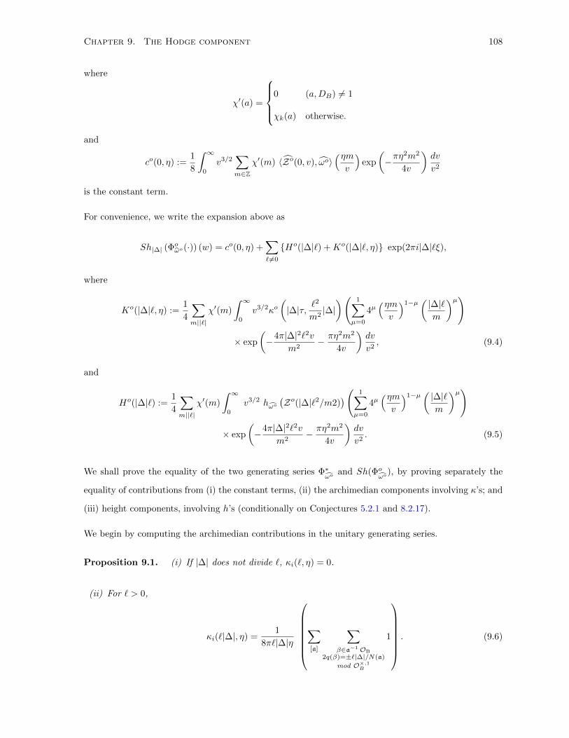
Chapter 9. The Hodge component 108
where
χ′(a) =
0 (a,DB) 6= 1
χk(a) otherwise.
and
co(0, η) :=1
8
∫ ∞0
v3/2∑m∈Z
χ′(m) 〈Zo(0, v), ωo〉(ηmv
)exp
(−πη
2m2
4v
)dv
v2
is the constant term.
For convenience, we write the expansion above as
Sh|∆| (Φoωo(·)) (w) = co(0, η) +
∑` 6=0
Ho(|∆|`) +Ko(|∆|`, η) exp(2πi|∆|`ξ),
where
Ko(|∆|`, η) :=1
4
∑m||`|
χ′(m)
∫ ∞0
v3/2κo(|∆|τ, `
2
m2|∆|)( 1∑
µ=0
4µ(ηmv
)1−µ(|∆|`m
)µ)
× exp
(−4π|∆|2`2v
m2− πη2m2
4v
)dv
v2, (9.4)
and
Ho(|∆|`) :=1
4
∑m||`|
χ′(m)
∫ ∞0
v3/2 hωo(Zo(|∆|`2/m2)
)( 1∑µ=0
4µ(ηmv
)1−µ(|∆|`m
)µ)
× exp
(−4π|∆|2`2v
m2− πη2m2
4v
)dv
v2. (9.5)
We shall prove the equality of the two generating series Φ∗ωo
and Sh(Φoωo
), by proving separately the
equality of contributions from (i) the constant terms, (ii) the archimedian components involving κ’s; and
(iii) height components, involving h’s (conditionally on Conjectures 5.2.1 and 8.2.17).
We begin by computing the archimedian contributions in the unitary generating series.
Proposition 9.1. (i) If |∆| does not divide `, κi(`, η) = 0.
(ii) For ` > 0,
κi(`|∆|, η) =1
8π`|∆|η
∑[a]
∑β∈a−1OB
2q(β)=±`|∆|/N(a)
mod O×,1B
1
. (9.6)

Chapter 9. The Hodge component 109
(iii) For ` < 0,
κi(`|∆|, η) =1
2
(1
4π|∆`|ηe−4π|∆`|ηs −
∫ ∞1
e−4π|∆`|ηs ds
s
)∑[a]
∑β∈a−1OB
2q(β)=±`|∆|/N(a)
mod O×,1B
1
. (9.7)
Proof. We may write
κi(`, η) =1
2
∫CB(C)
φ∗iGr(`, η) c1(ωo)
=1
2
∑[a]∈Cl(k)
∫[O×,1B \H]
[ ∑β∈a−1OB
2q(β)=`/N(a)
Gr+(
(2N(a)η)1/2β, φi(z))
+∑
β∈a−1OB
2q(β)=−`/N(a)
Gr−(
(2N(a)η)1/2β, φi(z))] 1
2π
dx ∧ dyy2
(9.8)
for the Green’s functions Gr±(β, ζ) defined in Section 3.5. We have also used the fact [16, Eqn. (3.16)] :
c1(ωo) =1
2π
dx ∧ dyy2
.
Let D(BR)− denote the space of negative definite kR-lines in BR, and fix an orthogonal basis v+, v−
for BR such that 2q(v+) = −2q(v−) = 1, and 〈v+, v−〉 = 0; here q(v) = |∆|Nrd(v). Upon identifying
kR ' C, we obtain an isomorphism
U1 := w ∈ C ||w| < 1 ' D(BR)− w ←→ spanw · v+ + v−.
In particular, as in the proof of Theorem 7.1), we obtain
c1(ωo) =2
πφ∗i
(r dr ∧ dθ(1− r2)2
),
where w = reiθ is the parameter on U1 described above.
We remark that as q(OB) ⊂ (|∆|/2)Z, it follows easily that κi(`, η) = 0 unless |∆| divides `; this proves
the first part of the proposition. We also note that for the action of O×,1B by right-multiplication on B,
the stabilizer of any β ∈ B× is trivial. Hence, using (9.8), and the fact
∫CB(C)
=
∫[O×,1B \H]
=1
2
∫O×,1B \H
,

Chapter 9. The Hodge component 110
we may write
κi(|∆|`, η) =1
4
[ ∑β∈a−1OB
2q(β)=`/N(a)
mod O×,1B
∫H
Gr+(
(2N(a)η)1/2β, φi(z)) 1
2π
dx ∧ dyy2
+∑
β∈a−1OB
2q(β)=−`|∆|/N(a)
mod O×,1B
∫H
Gr−(
(2N(a)η)1/2β, φi(z)) 1
2π
dx ∧ dyy2
]
Suppose ` > 0, and β ∈ a−1OB with 2q(β) = `|∆|/N(a). Then we have
1
2
∫H
φ∗iGr+(
(2N(a)η)1/2β, ·)c1(ωo)
=1
2π
∫U1
Gr+(
(2N(a)η)1/2β,w) 2r drdθ
(1− r2)2. (9.9)
Note that U(BR) acts transitively on D(BR)− ' U1, and the measure appearing in (9.9) is invariant for
this action. Since the integral is unchanged after replacing β by any U(BR)-translate, we may assume
without loss of generality that
β =
(`|∆|N(a)
)1/2
v+,
so unravelling definitions, we obtain
Gr+(
(2N(a)η)1/2β,w)
=
∫ ∞1
exp
(−4π`|∆|η |w|2
1− |w|2s
)ds
s.
Hence
(9.9) =1
2π
∫U1
∫ ∞1
exp
(−4π`|∆|η r2
1− r2s
)ds
s
2r drdθ
(1− r2)2
=
∫ ∞1
e4π|∆|`ηs(∫ 1
0
e−4π`|∆|ηs/(1−r2) 2r dr
(1− r2)2
)ds
s
=1
4π`|∆|η
∫ ∞1
ds
s2
=1
4π`|∆|η.
Similarly, for ` > 0 and β ∈ a−1OB with 2q(β) = −`|∆|/N(a), it follows by an analogous argument that
1
2
∫H
φ∗iGr−(
(2N(a)η)1/2β, ·)c1(ωo) =
1
4π`|∆|η
as well.
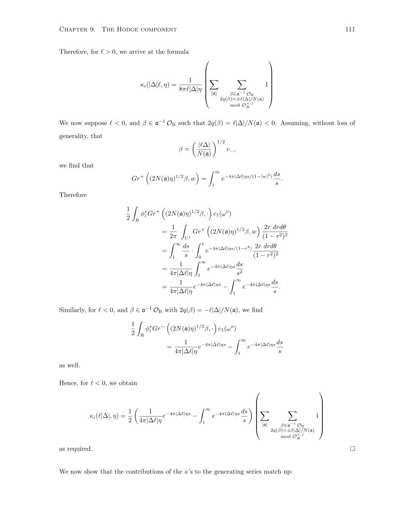
Chapter 9. The Hodge component 111
Therefore, for ` > 0, we arrive at the formula
κi(|∆|`, η) =1
8π`|∆|η
∑[a]
∑β∈a−1OB
2q(β)=±`|∆|/N(a)
mod O×,1B
1
We now suppose ` < 0, and β ∈ a−1OB such that 2q(β) = `|∆|/N(a) < 0. Assuming, without loss of
generality, that
β =
(|`∆|N(a)
)1/2
v−,
we find that
Gr+(
(2N(a)η)1/2β,w)
=
∫ ∞1
e−4π|∆`|ηs/(1−|w|2) ds
s.
Therefore
1
2
∫H
φ∗iGr+(
(2N(a)η)1/2β, ·)c1(ωo)
=1
2π
∫U1
Gr+(
(2N(a)η)1/2β,w) 2r drdθ
(1− r2)2
=
∫ ∞1
ds
s·∫ 1
0
e−4π|∆`|ηs/(1−r2) 2r drdθ
(1− r2)2
=1
4π|∆`|η
∫ ∞1
e−4π|∆`|ηs ds
s2
=1
4π|∆`|ηe−4π|∆`|ηs −
∫ ∞1
e−4π|∆`|ηs ds
s.
Similarly, for ` < 0, and β ∈ a−1OB with 2q(β) = −`|∆|/N(a), we find
1
2
∫H
φ∗iGr−(
(2N(a)η)1/2β, ·)c1(ωo)
=1
4π|∆`|ηe−4π|∆`|ηs −
∫ ∞1
e−4π|∆`|ηs ds
s
as well.
Hence, for ` < 0, we obtain
κi(`|∆|, η) =1
2
(1
4π|∆`|ηe−4π|∆`|ηs −
∫ ∞1
e−4π|∆`|ηs ds
s
)∑[a]
∑β∈a−1OB
2q(β)=±`|∆|/N(a)
mod O×,1B
1
as required.
We now show that the contributions of the κ’s to the generating series match up:

Chapter 9. The Hodge component 112
Theorem 9.2. Suppose |∆| is even, squarefree, and (|∆|, DB) = 1. Then for any ` 6= 0,
Ko(|∆|`, η) =1
h(k)|o×k |∑
[φi]∈Opt(ok,OB)
mod O×B
κi(`, η) e−2π|∆|`η.
In other words, the Archimedean components of Sh|∆|(Φoωo) and Φ∗ωo are equal.
Proof. We shall proceed by computing the (absolutely convergent) integrals appearing in (9.4), the
definition of Ko(|∆|`, η).
First consider the case ` 6= 0. In [16, Proposition 12.1], the authors provide a formula for the quantity
κo:
κo(|∆|τ, |∆|`2/m2
)=
∑x∈OB
x2=(`/m)2∆
modO×B
1
|Γx|·∫ ∞
0
e−4π|∆|2(`/m)2vs(
(s+ 1)1/2 − 1) dss
= 2∑x∈OB
x2=(`/m)2∆
modO×B
1
|Γx|·∫ ∞
1
exp(−4π|∆|2(`/m)2v(s2 − 1)
) s
s+ 1ds,
where Γx = γ ∈ O×B | γx = xγ.
Consider the integral∫ ∞0
v3/2κo(|∆|τ, |∆|`2/m2)
(1∑
µ=0
4µ(ηmv
)1−µ(|∆|`/m)µ
)
× exp
(−4π|∆|2r2v − πη2m2
4v
)dv
v2
= 2c(`/m)
∫ ∞0
v−1/2[ ∫ ∞
1
exp(−4π|∆|2(`2/m2)vs2
)( s
s+ 1
)ds]
×
(1∑
µ=0
4µ(ηmv
)1−µ(|∆|`/m)µ
)exp
(−πη
2m2
4v
)dv,
where
c(`/m) =∑x∈OB
x2=(`/m)2∆
modO×B
1
|Γx|.
Interchanging the order of integration and using the formulas (7.3) and (7.4), to evaluate the inner
integral on v, we find that the integral above is equal to
4c(`/m)I(`) := 4c(`/m)
∫ ∞1
(1 +
sgn(`)
s
)exp (−2π|∆||`|ηs)
(s
s+ 1
)ds.
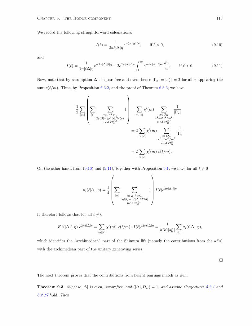
Chapter 9. The Hodge component 113
We record the following straightforward calculations:
I(`) =1
2π`|∆|ηe−2π|∆|`η, if ` > 0, (9.10)
and
I(`) =1
2π|`∆|ηe−2π|∆||`|η − 2e2π|∆||`|η
∫ ∞1
e−4π|∆||`|ηu du
u, if ` < 0. (9.11)
Now, note that by assumption ∆ is squarefree and even, hence |Γx| = |o×k | = 2 for all x appearing the
sum c(`/m). Thus, by Proposition 6.3.2, and the proof of Theorem 6.3.3, we have
1
2
∑[φi]
∑[a]
∑β∈a−1OB
2q(β)=±`|∆|/N(a)
mod O×,1B
1
=∑m||`|
χ′(m)∑x∈OB
x2=∆`2/m2
mod O×,1B
1
|Γx|
= 2∑m||`|
χ′(m)∑x∈OB
x2=∆`2/m2
mod O×B
1
|Γx|
= 2∑m||`|
χ′(m) c(`/m).
On the other hand, from (9.10) and (9.11), together with Proposition 9.1, we have for all ` 6= 0
κi(`|∆|, η) =1
4
∑[a]
∑β∈a−1OB
2q(β)=±`|∆|/N(a)
mod O×,1B
1
I(`)e2π|∆|`|η
It therefore follows that for all ` 6= 0,
Ko(|∆|`, η) e2π`|∆|η =∑m||`|
χ′(m) c(`/m) · I(`)e2π`|∆|η =1
h(k)|o×k |∑[φi]
κi(`|∆|, η),
which identifies the “archimedean” part of the Shimura lift (namely the contributions from the κo’s)
with the archimedean part of the unitary generating series.
The next theorem proves that the contributions from height pairings match as well.
Theorem 9.3. Suppose |∆| is even, squarefree, and (|∆|, DB) = 1, and assume Conjectures 5.2.1 and
8.2.17 hold. Then

Chapter 9. The Hodge component 114
(i) For ` 6= 0, if |∆| does not divide |`|, then hωo (φ∗i Z(`)) = 0.
(ii) For any ` 6= 0, we have
Ho(|∆|`) =1
h(k)|o×k |∑[φi]
hωo (φ∗i Z(|∆|`)) e−2π|∆|`η.
In particular, when ` < 0 both sides vanish.
Proof. First, we recall that by [17, Proposition 3.4.5], the orthogonal special cycles Zo(t) decompose
into substacks
Zo(t) = Zo(t)hor + Zo(t)ver,
where Zo(t)hor is the flat closure of the generic fibre Zo(t)Q, and Zo(t)ver is a cycle supported in the
fibres CBp at primes p|DB .
In particular, c.f. [16, p. 42], we find
hωo (Zo(t)) = hω0
(Zo(t)hor
)+∑p|DB
hω0 (Zo(t)p) ,
where Zo(t)p = Zo(t)ver ×Z Zp.
For any optimal embedding φ : ok → OB, the pullback cycles φ∗Z(m) can also be decomposed into
substacks in exactly the same way, by Conjecture 5.2.1.
Next, we note that we may decompose the cycles Zo(t)hor into horizontal integral substacks parametrized
by points on its generic fibre:
Zo(t)hor =∑
x∈Zo(t)horQ
Zx,
where x is the generic point of Zx, counted with multiplicities, and so by linearity,
hωo(Zo(t)hor
)=
∑x∈Zo(t)horQ
hωo (Zx) .
Similarly,
hωo(φ∗Z(m)hor
)=
∑y∈φ∗ Z(m)horQ
hωo (Zy) .
In particular, as q(OB) ⊂ |∆|Z, we have that φ∗Z(`)hor(C) is empty whenever |∆| does not divide `,
proving the first part of the statement, for the horizontal contributions.
On the other hand, for ` > 0, ` ∈ |∆|Z, we have already shown the relation (Theorem 6.3.3):∑m|`
χ′(`)Zo(|∆|`2/m2)Q =1
h(k)|o×k |∑[φi]
φ∗i Z(`|∆|)Q. (9.12)

Chapter 9. The Hodge component 115
Recall the definition
Ho(|∆|`) :=1
4
∑m||`|
χ′(m)
∫ ∞0
v3/2 hωo(Zo(|∆|`2/m2)
)( 1∑µ=0
4µ(ηmv
)1−µ(|∆|`m
)µ)
× exp
(−4π|∆|2`2v
m2− πη2m2
4v
)dv
v2.
We note the identity:∫ ∞0
v3/2
(1∑
µ=0
4µ(ηmv
)1−µ(|∆|`/m)µ
)exp
(−4π|∆|2r2v − πη2m2
4v
)dv
v2
= 2 (1 + sgn(`)) e−2π|∆||`|η,
and so, for the contributions of the horizontal cycles, we have
Ho(|∆|`)hor =∑m|`
χ′(m) hωo(Zo(|∆|`2/m2)hor
)e−2π|∆|`, ` > 0,
and Ho(|∆|`)hor = 0 for ` < 0; this yields the desired identity for the horizontal contributions.
Turning to the vertical contributions at primes p|DB , note that if we replace Zo(t) with Z
o(t)pure as in
[17, pp. 54-55], then the contributions to the height pairing remains unchanged.
The desired relation then follows by the same argument as above, with Conjecture 8.2.17 taking the
place of (9.12) above.
Finally, it remains to compare the constant terms:
Proposition 9.4.
co(0, η) =1
h(k)|o×k |∑[φi]
〈φ∗Z(0, η), ωo〉
Proof. We begin by manipulating the expression for the constant term of the Shimura lift of the orthog-
onal generating series:
co(0, η) =1
8
∫ ∞0
v3/2〈Zo(0, v), ωo〉∑m∈Z
χ′(m)(ηmv
)exp
(−πη
2m2
4v
)dv
v2
=1
4
∫ ∞0
〈Zo(0, 1/u2), ωo〉 ·∑m∈Z
χ′(m)(ηm) exp
(−πη
2m2u2
4
)du.
To help our formulas appear somewhat neater, let D = DB and t = |∆|.

Chapter 9. The Hodge component 116
Applying twisted Poisson summation to the inner sum on m, c.f. [4, Eqn. 2.42], yields:∑m∈Z
χ′(m) m exp
(−πη
2m2u2
4
)
=−i
2D2t2· 1
η3u3
[∑m∈Z
χ′(m)m exp
(− πm2
4D2t2η2u2
)],
where
χ′(m) =
4Dt∑a=1
χ′(a) e(am/4Dt).
Substituting this back in and applying a change of variables yields
co(0, η) =−i
8D2t2
∫ ∞0
〈Zo(0, 1/u2), ωo〉 · 1
η2u2
∑m∈Z
χ′(m)m exp
(−πm2
4D2t2η2u2
)du
u
=−i4
∫ ∞0
∑m∈Zm6=0
〈Zo(0, 4D2t2η2u/m2
), ωo〉 · χ′(m) m−1 exp(−πu) du.
Recall that we had defined
Zo(0, v) = −ωo − (0, log(v))− (0, log(D)) ∈ CH1(CB)R,
and hence
〈Zo(0, 4D2t2η2u/m2
), ωo〉 = −〈ωo, ωo〉 − deg(ωo)
2
[log u+ log(4D2t2η2)− 2 logm+ logD
].
Plugging this back into our expression for the constant term yields:
co(0, η) =i
2
(〈ωo, ωo〉+
deg(ωo)
2log(4η2D3t2)
)(∫ ∞0
e−πudu
)L(1, χ′)+
+i
2
(deg(ωo)
2
)(∫ ∞0
log(u)e−πudu
)L(1, χ′)
+i
2
(deg(ωo)
2
)(∫ ∞0
e−πudu
)(2L′(1, χ′))
=i
2π
[〈ωo, ωo〉+
deg(ωo)
2
(log(4η2D3t2/π)− γ
)]L(1, χ′)
+i
2πdeg(ωo)L′(1, χ′),
where γ is the Euler-Mascheroni constant.
It now follows, essentially by definition, c.f. (5.2.2), that
1
h(k)|o×k |∑[φi]
〈φ∗i Z(0, η), ωo〉 = co(0, η),
as required.

Bibliography
[1] R. Borcherds, The Gross-Kohnen-Zagier theorem in higher dimensions. Duke J. Math., 97 (1999).
pp. 219-233.
[2] J.-F. Boutot and H. Carayol, Uniformisation p-adique des courbes de Shimura: les theoremes de
Cerednik et de Drinfeld. Courbes modulaire et courbes de Shimura, Asterisque 196-197 (1991), pp.
45-158.
[3] C.L. Chai and F. Oort, Moduli of abelian varieties and p-divisible groups, in Arithmetic Geometry,
Clay Math. Proc., 8 (2009). pp. 441-536.
[4] B. Cipra, On the Niwa-Shintani theta-kernel lifting of modular forms. Nagoya Math. J., 91 (1983),
pp. 49-117.
[5] S. Friedberg, On the imaginary quadratic Doi-Naganuma lifting of modular forms of arbitrary level.
Nagoya Math. J., 92 (1983), pp. 1-20.
[6] I.S. Gradshteyn and I.H. Ryzhik, Tables of Integrals, Series and Products. Academic Press, 5th ed.
Allan Jeffrey, ed. (1995).
[7] F. Hirzebruch and D. Zagier, Intersection numers of curves on Hilbert modular surfaces and modular
forms of Nebentypus. Invent. math., 36 (1976), pp. 57-113.
[8] B. Howard, Complex multiplication cycles and Kudla-Rapoport divisors, to appear in Ann. of Math.
[9] B. Howard, Intersection theory on Shimura surfaces. Compos. Math. 145, 2 (2009), 423-475.
[10] H. Kojima, Shimura correspondence of Maass wave forms of half integral weight. Acta Arithmetica,
69 (1995), pp. 367-385.
117
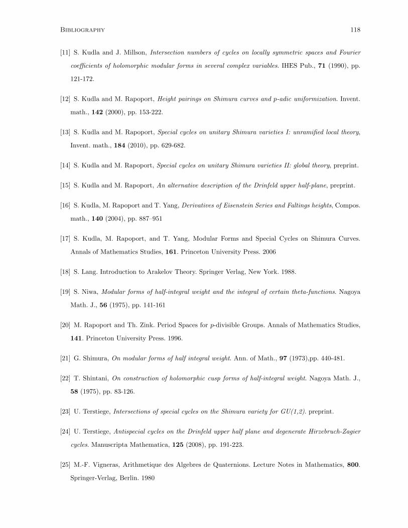
Bibliography 118
[11] S. Kudla and J. Millson, Intersection numbers of cycles on locally symmetric spaces and Fourier
coefficients of holomorphic modular forms in several complex variables. IHES Pub., 71 (1990), pp.
121-172.
[12] S. Kudla and M. Rapoport, Height pairings on Shimura curves and p-adic uniformization. Invent.
math., 142 (2000), pp. 153-222.
[13] S. Kudla and M. Rapoport, Special cycles on unitary Shimura varieties I: unramified local theory,
Invent. math., 184 (2010), pp. 629-682.
[14] S. Kudla and M. Rapoport, Special cycles on unitary Shimura varieties II: global theory, preprint.
[15] S. Kudla and M. Rapoport, An alternative description of the Drinfeld upper half-plane, preprint.
[16] S. Kudla, M. Rapoport and T. Yang, Derivatives of Eisenstein Series and Faltings heights, Compos.
math., 140 (2004), pp. 887–951
[17] S. Kudla, M. Rapoport, and T. Yang, Modular Forms and Special Cycles on Shimura Curves.
Annals of Mathematics Studies, 161. Princeton University Press. 2006
[18] S. Lang. Introduction to Arakelov Theory. Springer Verlag, New York. 1988.
[19] S. Niwa, Modular forms of half-integral weight and the integral of certain theta-functions. Nagoya
Math. J., 56 (1975), pp. 141-161
[20] M. Rapoport and Th. Zink. Period Spaces for p-divisible Groups. Annals of Mathematics Studies,
141. Princeton University Press. 1996.
[21] G. Shimura, On modular forms of half integral weight. Ann. of Math., 97 (1973),pp. 440-481.
[22] T. Shintani, On construction of holomorphic cusp forms of half-integral weight. Nagoya Math. J.,
58 (1975), pp. 83-126.
[23] U. Terstiege, Intersections of special cycles on the Shimura variety for GU(1,2). preprint.
[24] U. Terstiege, Antispecial cycles on the Drinfeld upper half plane and degenerate Hirzebruch-Zagier
cycles. Manuscripta Mathematica, 125 (2008), pp. 191-223.
[25] M.-F. Vigneras, Arithmetique des Algebres de Quaternions. Lecture Notes in Mathematics, 800.
Springer-Verlag, Berlin. 1980

Bibliography 119
[26] A. Vistoli, Intersection theory on algebraic stacks and their moduli spaces. Invent. math., 97 (1989),
pp. 613-670
[27] L. Washington, Introduction to Cyclotomic Fields. Graduate Texts in Mathematics, 83. Springer-
Verlag, New York. 1982.


