

Specialization Dynamics and Idea Flows∗
Preliminary and Incomplete Draft, Please Do Not Cite
Liuchun Deng†
June 29, 2016
Abstract
This paper studies the dynamics of international trade from the perspective of technol-
ogy diffusion. I build into an idea-flow model the sectoral dimension. The cross-sectional
setting is a fully-fledged Ricardian model with multiple factors and input-output linkages.
Sectoral productivity, as well as factor endowment, shapes specialization pattern across
countries. Driven by knowledge diffusion, comparative advantage evolves over time. By
putting sectors into play, I integrate four channels of idea flows: each firm could learn
from domestic producers as well as foreign sellers, and technology spillover is both intra-
industry and inter-industry. The theoretical framework yields a system of law of motion
of sectoral productivity across countries, capturing strong interdependence of the evolution
of comparative advantage. Based on the law of motion, my empirical exercise quantifies
the contribution of different channels of knowledge diffusion to dynamics of trade. My
quantitative results reproduce important patterns in the data: strong unconditional con-
vergence, substantial mobility in specialization, hyper-specialization. The calibrated model
also gives rise to a complex network of cross-country cross-industry knowledge spillover.
Various measures based on the network structure are proposed to identify the “key player”
in global diffusion of ideas.
Keywords: International trade, specialization dynamics, sectoral productivity, com-
parative advantage, technology diffusion, economic growth
JEL Classification: F10, F43, O33, O47
∗I am grateful to Pravin Krishna, M. Ali Khan, and Heiwai Tang for their continued support and encourage-ment. I wish to thank Lawrence Ball, Olivier Jeanne, Anton Korinek, Felipe Saffie, Mine Senses, Boqun Wang,Jonathan Wright, and Jiaxiong Yao along with seminar participants at the Johns Hopkins University for veryhelpful comments. All errors are mine.†Department of Economics, The Johns Hopkins University. E-mail [email protected]
1

1 Introduction
The last few decades have painted an intriguing picture of specialization dynamics. A number of
economies have experienced dramatic change of their export baskets. China’s top export industry
shifted from children’s toys to computers within less than twenty years (Hanson, 2012). Since
1970s, South Korea has managed to become one of the major players in shipbuilding industry
from scratch. Frequent turnover of main export industries is not just confined to Eastern Asian
miracle economies. African countries have also witnessed high turnover of their main exporting
industries in the last two decades (Easterly and Reshef, 2010), accompanied with spectacular
growth rates of these economies (Young, 2012).
Specialization pattern and industrial growth is interrelated in an interdependent world. Does
technology diffusion serve as a plausible explanation of specialization dynamics? If the answer
is affirmative, through what channel does technology diffusion drive specialization dynamics?
Moreover, does specialization pattern also shape the pattern of technology diffusion? If the
answer is affirmative, through what channel? This paper studies the complex two-way relation-
ship between international trade and economic growth through the lens of knowledge diffusion,
thereby shedding light on the sources of evolving comparative advantage.
This paper builds into an idea-flow model (Buera and Oberfield, 2016) the sectoral dimension.
The cross-sectional setting is a fully-fledged Ricardian model with multiple factors and input-
output linkages in light of Caliendo and Parro (2014) and Levchenko and Zhang (2015). Sectoral
productivity, as well as factor endowment, shapes specialization pattern across countries. Driven
by knowledge diffusion, comparative advantage evolves over time. By putting sectors into play, I
am able to integrate four channels of idea flows: each firm could learn from domestic producers
as well as foreign sellers, and technology spillover is both intra- and inter- sector. The theoretical
framework yields a system of law of motion of sectoral productivity across countries, capturing
strong interdependence of the evolution of comparative advantage.
The law of motion of sectoral productivity is amenable for empirical implementation. Using
production and trade data, I fully estimate and calibrate this structural model of technology
diffusion. The empirical exercise answers three broadly related questions that have important
policy implications. First of all, it offers a tentative answer to a longstanding question in the
literature on economic growth: international technology diffusion explains a great deal of uncon-
ditional convergence at the sector level. Beyond many existing theoretical studies, the simulated
trade pattern produced by my model quantitatively matches the convergence pattern under var-
ious specifications suggested by the literature. Moreover, sectoral concentration, comovement
pattern of export baskets, and transition dynamics implied by the simulated model is broadly
consistent with actual trade pattern. Second, my empirical analysis quantifies and compares the
2

contribution of each channel of technology diffusion to the sector-level productivity growth across
countries. In our sample of 32 OECD countries and 40 non-OECD countries, international tech-
nology diffusion on average plays a much more important role than domestic technology diffusion
on the evolution of Ricardian comparative advantage. This result stands sharp contrast with
Keller (2002b) whose empirical analysis is mainly based on R&D data and thereby restricted
within a small set of industrialized economies. A bulk of the literature focuses exclusively on
international knowledge diffusion, nevertheless being silent on domestic diffusion of technology
after its initial localization. My empirical exercise tries to fill this void by offering a model-based,
sector-specific comparison of international versus domestic knowledge diffusion. Intra-sector tech-
nology diffusion accounts for about 70% of productivity growth, while inter-sector technology
diffusion, a channel that receives much less attention in growth models, accounts for the rest
30% of productivity growth. Last, based on the calibrated diffusion model, I construct a matrix
of knowledge flow as opposed to the flow of goods directly observed from trade data. Using the
full structure of knowledge flow, I identify the “key player” in the global technology diffusion,
that is, the country (or country-industry pair) that contributes most to the global productivity
growth.
Relation to the Literature
This paper is motivated by two overarching facts. Proudman and Redding (2000) and Redding
(2002) document substantial mobility of specialization patterns across a few OECD countries
and the degree of international specialization does not increase over time. In a recent work,
Hanson and Muendler (2014) find surprisingly high turnover rates of top exporting industries
among a wide range of countries over medium and long run. On the other hand, unconditional
convergence has returned in favor of the conventional wisdom: a laggard country tends to achieve
higher productivity growth provided that it has access to the same technology as advanced
economies. At the product level, Hwang (2006) documents widespread convergence in product
quality proxied by unit values. Rodrik (2013b) offers convincing evidence that productivity
unconditionally converges at different levels of aggregation within the manufacturing sector.
Based on a structural trade model, Levchenko and Zhang (2015) document that within a country
less productive industries on average enjoy higher productivity growth1. My paper joins this
broad literature by quantifying the impact of various channels of knowledge diffusion on the
evolution of comparative advantage.
From a theoretical perspective, this paper is directly related to the recent theoretical literature
of “idea flows”. In these models, agent-to-agent (or firm-to-firm) interaction is the engine of
1Sharing similar insight with Levchenko and Zhang (2015), Fadinger and Fleiss (2011) also estimate sectoralproductivity using trade and production data.
3

growth (Lucas and Moll, 2014; Perla and Tonetti, 2014). Each period, an agent is randomly
matched with another agent in the economy and potentially adopts the new insight from the
matched agent. Economic growth is thereby characterized by a traveling wave of productivity
distribution within the economy. Extending this framework into the open-economy setting, a
series of theoretical work studies how dynamic gains from trade arise from learning from foreign
sellers (Alvarez et al., 2013), change of timing of technology adoption (Perla et al., 2015), and
dynamic selection effects due to entry-exit decision (Sampson, 2014). My model builds upon ?
which itself nests Kortum (1997) and Alvarez et al. (2013). The key departure from ? is to open
up the industry dimension Agents across different industries are allowed to meet each other and
exchange insights. The traveling wave of an industry is thereby determined by probability of
random meetings and relative quality of new insights, while the latter is further determined by
comparative advantage of industry productivity.
The cross-sectional setting of my model closely follows Levchenko and Zhang (2015). Origi-
nating from Eaton and Kortum (2002), a large literature employs quantifiable trade models to
study how Ricardian comparative advantage shapes international trade. Costinot et al. (2012)
first extend the Eaton-Kortum framework into a multi-industry setting to explore Ricardo’s origi-
nal insights: a country’s export basket is determined by its comparative advantage. Caliendo and
Parro (2014) and Levchenko and Zhang (2015) further extend the framework by incorporating
input-output linkages and multiple factors of production. Though their theoretical predecessors
are dynamic growth models (Kortum, 1997; Eaton and Kortum, 1999), most of the existing
structural trade models are static. By incorporating the time dimension, this paper goes beyond
comparative statics.
This paper is also related to an earlier literature of international technology diffusion2. This
strand of literature studies the extent to which technology diffuses across borders via imports,
exports, and foreign direct investment. A prominent example is Coe and Helpman (1995). They
document that a country’s R&D expenditures have large effects on productivity of its trade
partners. Keller (2002a) further demonstrates international spillover of R&D expenditures is
largely localized and correlated with non-trade variables such as language. Much of the existing
empirical analysis relies on availability of cross-country sectoral R&D data, and as a result, focus
has been put on a small sample of industrialized economies. To motivate empirical framework,
the existing work typically draws insights from innovation-based growth models, synthesized by
Grossman and Helpman (1993). In contrast, this paper complements the literature by taking
a different theoretical perspective. Although this paper is agnostic about sources of knowledge
creation, it introduces a much finer process of knowledge diffusion micro-founded by firm-to-firm
interactions. By focusing on the very nature of technology spillover, my theoretical framework is
2Keller (2004) provides an excellent review.
4

more suitable for analyzing technology catchup of the developing world where most countries are
technology recipients rather than creators. Because the law of motion of sectoral productivity
derived in this paper depends exclusively on variables that can be constructed by using only trade
and production data, I am also freed from using R&D data and therefore a much larger sample
of developing countries can be included in my sample. Moreover, the merit of this diffusion
framework is its tight connection to empirics. Beyond motivational purpose, the theoretical
results will be used to discipline the empirical implementation.
Keller (2002b) also integrates intra- and inter- industry spillover both internationally and
domestically in shaping a country’s sectoral productivity. As a common empirical approach,
he examines industry-level total factor productivity (henceforth TFP) in relation to domestic
and foreign R&D expenditures across different industries. However, my work distinguishes from
Keller (2002b) by investigating growth rates rather than level terms of TFP. In this sense, Keller
(2002b) is inherently static by focusing on steady states of world productivity distribution, while
my work takes a dynamic perspective by focusing on transitional dynamics of world productivity
growth.
My empirical analysis yields an estimated network of industry knowledge diffusion. This
contributes to the literature that examines economic consequences of technological relatedness
of industries starting from Jaffe (1986). Based on co-export structure, Hidalgo et al. (2007)
formalize the concept of the “product space” and document strong path dependence of trade
patterns. Follow-up work by Kali et al. (2012) study the structure of the product space in
relation to economic growth using cross-country regressions. Cai and Li (2014) builds into an
innovation-based growth model sectoral linkages of knowledge creation. Using patent citation
data, they demonstrate that sectoral linkage is important in explaining firms’ patenting behavior.
A common feature of the existing work is that relatedness of industries is treated as input rather
than output in empirical analysis. In contrast, the network of industry knowledge diffusion is
structurally estimated in this paper, so it can be potentially used in the future research as a
model-based alternative to those reduced-form technology flow matrices.
Lastly, this paper is related to the discussion of trade and industrial policies. As a seminal
work, Hausmann and Rodrik (2003) highlight the problem of appropriability associated with
localizing foreign technology. On the contrary, recent case studies on export pioneers (Sabel
et al., 2012) suggest that coordination problem is the foremost issue of initiating new export
activities. This paper takes a macro perspective on diffusion barriers by offering a systematic
sector-level comparison between international and domestic knowledge spillover. A related but
more controversial discussion is about whether what a country exports matters for its future
economic growth. Cross-country regressions by Hausmann et al. (2007) suggest that a country
tends to achieve higher economic growth if its export basket biases towards those of rich coun-
5

tries. This finding spurs a huge debate on industrial policy3. My work joins this debate by
quantitatively investigating how a country’s production structure and import bundles impact its
sectoral productivity growth.
The rest of the paper is structured as follows. Section 2 presents a set of motivating evidences:
unconditional convergence, high turnover rate of export industries, and comovement of export
baskets between geographical neighbors. Section 3 describes the model, solves the instantaneous
equilibrium and derives the law of motion of sectoral productivity. Section 4 discusses sample
construction and my two-step estimation strategy. Section 5 presents main results and demon-
strates the internal validity of the model. Section 6 performs counter-factual analysis. Section 7
concludes.
2 Motivating Evidence
2.1 Unconditional Convergence
Despite negative findings of unconditional convergence at the aggregate level, the recent literature
suggests that within the manufacturing sector countries (or industries) tend to achieve higher
productivity growth if the initial level of productivity is relatively low Rodrik (2013a). Figure
1 illustrates unconditional convergence from a slightly different view. I plot industry-level TFP
grow rates in the tradeable sector from 1960 to 2000 against the gap between a country’s TFP
and average TFP of its trade partners weighted by import shares in 1960. There is clearly a
negative relationship between the growth rate and the initial gap. It suggests that a country’s
industrial productivity converges to not only the world technology frontier that is documented in
the literature but also its trade partners’ productivity levels. International technology diffusion,
or more specifically, learning from trade partners seems to be a plausible explanation of this
convergence effect. In the next section, I build up a model of technology diffusion to quantitatively
access how various channels of technology diffusion could give rise to unconditional convergence.
[Figure 1 about here.]
2.2 Specialization Dynamics
The second evidence is inherently related to unconditional convergence. Sectoral productivity
dynamics can lead to specialization dynamics due to change of Ricardian comparative advantage.
Earlier work by Redding (2002) examines evolution of export baskets of seven OECD countries.
Employed with an empirical framework of distribution dynamics, he finds substantial mobility
3A collection of critique can be found in Lederman and Maloney (2012).
6

in specialization. This finding is further extended by Hanson and Muendler (2014) in a gravity-
equation framework. In a 20-year window, they find the turnover rate of the top 5% industries
is about 60%. These findings stay in stark contrast with theory, because existing trade models
are mostly static and the few exceptions typically focus on balanced growth path. To explain
specialization dynamics, especially to account for the high degree of mobility, a model needs to
have two key features: comparative advantage is itself endogenously determined and evolves over
time; transition dynamics is amenable for empirical implementation.
2.3 Comovement Pattern
Another interesting feature of evolving comparative advantage is that neighboring countries tend
to have similar export baskets and more importantly their export baskets tend to be increasingly
similar. In Figure 2, I plot how correlation of industry-level export shares between geographical
neighbors evolves over time. Among four pairs (Chile vs Peru, South Korea vs Japan, Mex-
ico vs USA, and Saudi Arabia vs Egypt), correlation moves generally upward in the post-war
era. Regression results in Bahar et al. (2013) confirms that a country tends to enjoy faster
export growth in industries where its neighbors have established comparative advantage. This
neighboring effect again suggests that international technology diffusion may be in effect. In
the quantitative analysis of my model, I will test if technology diffusion could result in similar
comovement patterns.
[Figure 2 about here.]
3 Model
My model has two main components. The cross-sectional setting is a multi-sector multi-country
Hechscher-Ohlin-Ricardian framework with sectoral linkages, which closely follows Caliendo and
Parro (2014) and Levchenko and Zhang (2015). Dynamics of sectoral productivity is modeled
in line with Buera and Oberfield (2016). Diffusion of ideas is the engine of productivity growth.
Two-way relationship between international trade and productivity growth is separated into
two dimensions: at each moment of time, the trade pattern is determined by cross-country
sectoral productivity; along the time dimension, productivity growth is shaped by the pattern of
international trade. By incorporating the sectoral dimension into Buera and Oberfield (2016), I
am able to investigate a rich set of knowledge diffusion and derive the law of motion for sectoral
productivity that is amenable to empirical implementation.
In my model, the world consists of N countries indexed by n and n′. There are I + 1 sectors
indexed by i and i′ among which the first I sectors produce tradeable goods and the (I + 1)-th
7
sector produces non-tradeable goods. Time is continuous, infinite, and indexed by t.
3.1 Cross-sectional Setup
To simplify the notation, I suppress the time subscript “t” in presenting the cross-sectional setup.
3.1.1 Demand
Goods from I + 1 sectors are combined into final goods which are used for investment and final
consumption. The combination is of the form
Yn(Y 1n , Y
2n , ..., Y
I+1n ) =
[I∑i=1
(ωin)1−κ (
Y in
)κ]φn/κ (Y I+1n
)1−φn,
where Yn is the output of final goods in country n and Y in is the goods from industry i, ωin is the
share parameter of tradeable goods and∑I
i=1 ωin = 1 for any country n; φn is country-specific
Cobb-Douglas share of tradeable goods; the elasticity of substitution across tradeable goods is
given by 1/(1−κ). Therefore, a representative consumer in country n is faced with the following
per-period decision problem
maxY 1n ,Y
2n ,...,Y
I+1n
Yn(Y 1n , Y
2n , ..., Y
I+1n ) subject to
I+1∑i=1
P inY
in ≤ En,
where P in is the sectoral price index and En is per-period total expenditure. Therefore,
consumers have two-tier preferences: the first tier is Cobb-Douglas between tradeable and non-
tradeable sectors and the second tier exhibits constant elasticity of substitution (CES henceforth)
across I tradeable sectors. Standard derivation yields
Y in =
ωinPin
κκ−1∑I
i′=1 ωi′nP
i′n
κκ−1
· φnEnP in
, i = 1, 2, ..., I, (1)
Y I+1n =
(1− φn)EnP I+1n
. (2)
3.1.2 Production
In each sector i, there is a unit mass of intermediate goods indexed by νi ∈ [0, 1]. Each variety
of intermediate good νi is produced by using labor, capital, and composite intermediate goods.
8

Production technology is of Cobb-Douglas form
qin(νi) = zin(νi)[`in(νi)]γiL
[kin(νi)]γiK
I+1∏i′=1
[mii′
n (νi)]γii′n ,
where qin(νi) is the output of variety νi; zin(νi) is the productivity level; `in(νi) and kin(νi) are labor
and capital; mii′n is composite intermediate goods from industry i′; Cobb-Douglas coefficients γiL
and γiK are the labor and capital shares; γii′
n is the share of intermediate goods from sector i′,
capturing the important sectoral input-output (I-O henceforth) linkage that is emphasized by
the recent macroeconomics literature (Carvalho, 2014). Production technology follows constant
returns to scale (CRS henceforth), which requires γiL + γiK +∑I+1
i′=1 γii′n = 1 for any country n.
According to the production function, the unit cost of an input bundle cin can be defined as
cin =
(wnγiL
)γiL (rnγiK
)γiK I+1∏i′=1
(P i′n
γii′n
)γii′n, (3)
where wn is the wage rate and rn is the rental rate.
Composite goods in each industry are produced by combining a continuum of varieties within
the same industry. Production technology is of CES form
Qin =
[∫ 1
0
qin(νi)(σi−1)/σidνi
]σi/(σi−1),
where σi is the elasticity of substitution. Standard derivation yields
qin(νi) =
(pin(νi)
P in
)−σiQin,
with
P in =
[∫ 1
0
pin(νi)1−σi
dνi]1/(1−σi)
,
where pin(νi) is the price of variety νi in country n.
Composite goods in each sector can be used as either intermediate goods for domestic pro-
duction or production of final consumption goods. Production technology of composite and final
goods is identical across countries. It implies that international trade only occurs at the variety
level, which will be specified in the next section.
9

3.1.3 International Trade
Trade cost is of the iceberg form (Samuelson, 1954). It requires shipping dinn′ units of goods
from country n′ to deliver one unit of good to country n. The triangle inequality is assumed to
always hold: dinn′′din′′n′ ≥ dinn′ for any country n, n′, n′′ and sector i. It implies re-export is always
more costly than direct export in the model, and consequently trade hubs like Singapore and
Hong Kong are excluded in the empirical implementation of the model. For the non-tradeable
sector, dI+1nn′ = ∞ for any n, n′ such that n 6= n′. Domestic trade is assumed to be frictionless4,
so dinn = 1 for any n and i.
The product market is assumed to be perfectly competitive. Each variety of intermediate
inputs is purchased from the supplier with the lowest unit cost adjusted by trade cost. Recall
that cin is the unit cost of an input bundle of sector i in country n. Therefore, price of the
intermediate good νi in country n is given by
pin(νi) = min
{ci1d
in1
zi1(νi),ci2d
in2
zi2(νi), ...,
ciNdinN
ziN(νi)
}.
Following Eaton and Kortum (2002), variety-level productivity zin is a random draw from a
Frechet distribution given by
F in(z) = exp(−λinz−θ
i
).
where F in is country n’s productivity distribution in sector i; the location parameter λin governs
the mean of distribution; θi measures the dispersion of the distribution. Denote by πinn′ the share
of expenditure that country n spends on the imports from country n′ in sector i. Utilizing the
probabilistic structure, standard derivation yields
πinn′ =λin′(c
in′d
inn′)
−θi∑Nn′′=1 λ
in′′(c
in′′d
inn′′)
−θi, (4)
where the denominator captures “multilateral resistance” coined by Anderson and van Wincoop
(2003), that is, the fact that bilateral trade flows are shaped by economic variables beyond
those of the bilateral trading partners in a multilateral world. The sectoral price index is also
determined by the multilateral resistance terms
P in =
[Γ
(1 +
1− σi
θi
)]1/(1−σi)( N∑n′=1
λin′(cin′d
inn′)
−θi)−1/θi
, (5)
4The recent work by Ramondo et al. (2016) suggests that assuming each country being fully integrated maynot be innocuous.
10

where Γ(·) is the Gamma function. The usual regularity condition θi + 1 > σi is imposed, so the
price index is well defined.
Note that the location parameter λin varies across time t. When turning to the time dimension
of the setup, I will use the learning process introduced by Buera and Oberfield (2016) to further
endogenize and dynamize the sectoral productivity distribution.
3.1.4 Market Clearing and Instantaneous Equilibrium
Denote country n’s total trade deficit by Dn. Like Caliendo and Parro (2014), I allow interna-
tional lending and borrowing, and trade deficits are exogenously given. The world-total trade
deficit has to be balanced out, so∑N
n=1Dn = 0. Country n’s expenditure is therefore given by
En = wnLn + rnKn +Dn, (6)
where Ln and Kn is labor and capital endowment.
By definition, the trade deficit is the difference between total imports and exports
Dn =I+1∑i=1
(P inQ
in −
N∑n′=1
P in′Q
in′π
in′n
)(7)
Recall that the sectoral composite goods can be used for either intermediate goods or final
consumption goods, so the product market clearing condition in each sector is given by
P inQ
in =
I+1∑i′=1
γi′in
N∑n′=1
P i′
n′Qi′
n′πi′
n′n + P inY
in (8)
Given the Cobb-Douglas production function, the share of labor and capita income within
each sector is given by γiL and γiK , respectively. Therefore, I have
wnLin = γiL
N∑n′=1
P in′Q
in′π
in′n (9)
rnKin = γiK
N∑n′=1
P in′Q
in′π
in′n, (10)
where Lin and Kin are sector-level labor and capital.
11

Market clearing conditions for labor and capital markets further require
I+1∑i=1
Lin = Ln (11)
I+1∑i=1
Kin = Kn. (12)
At each moment of time t, given labor and capital endowment {Ln}Nn=1 and {Kn}Nn=1, trade
deficits {Dn}Nn=1, bilateral sector-level trade costs {dinn′}N,N,I+1n=1,n′=1,i=1, and sectoral productivity
measures {λin}N,I+1n=1,i=1, an instantaneous equilibrium is characterized by {rn}Nn=1, {wn}Nn=1, and
{P in}
N,I+1n=1,i=1 such that consumers maximize utility (Equation 1, 2), firms maximize profit (Equa-
tion 3), decision on international trade is made optimally (Equation 4, 5), product markets clear
(Equation 6 - 8), and factor markets clear (Equation 9 - 12), or in short, Equation 1 - 12 hold5
for any country n and sector i.
3.2 Dynamic Setup
3.2.1 A General Learning Process
I start with a brief description of a general learning process originally formulated by Buera and
Oberfield (2016). Technology advances through adopting new ideas. Arrival of new ideas is
modeled as a Poisson process with rate η. Upon arrival of a new idea, the producer compares the
productivity level of her technology with the realized productivity of the new idea. Productivity
level associated with each new idea, zG, is drawn from a source distribution Gin,t(·). The source
distribution evolves over time and potentially varies across countries and sectors. I will explicitly
specify the source distribution when turning to explain different channels of knowledge diffusion.
Producers are faced with uncertainty when adopting new ideas. Randomness of adoption effi-
ciency is captured by another random draw, zH , from an exogenous, time-invariant distribution
H i(·). In particular, the actual productivity of a new idea is given by a Cobb-Douglas combina-
tion of these two draws, zβi
G z1−βiH . The new idea is adopted if and only if zβ
i
G z1−βiH is greater than
the productivity level of the existing technology z. This process of adopting new ideas yields the
following law of motion of sectoral productivity distribution F in,t
d
dtlnF i
n,t(z) = −η∫ ∞0
[1−Gi
n,t
(z1/β
i
x(1−βi)/βi
)]dH i(x).
5Among these equations, N equations are redundant due to the income-expenditure identity for each country.Proof can be found in Appendix B.1.
12

Following Buera and Oberfield (2016), I assume that H i(·) follows a Pareto distribution,
H i(z) = 1− (z/z0)−θi , for z > z0. Let θi ≡ θi/(1− βi) and normalize η ≡ ηzθ0 to be a constant.
It can be further shown that
limz0→0
d
dtlnF i
n,t(z) = −ηz−θi∫ ∞0
xβiθidGi
n,t(x),
provided that limx→∞[1−Gin,t(x)]xβ
iθi = 0.
Therefore, I obtain the following sectoral productivity distribution
F in,t(z) = exp(−λin,tz−θ
i
),
with the law of motion of the key productivity parameter λin,t
dλin,tdt
= η
∫ ∞0
xβiθidGi
n,t(x).
Notice that the sectoral productivity distribution above coincides with the Frechet distribution
that I assume in the cross-section setting. In this sense, the general learning process endogenizes
the sectoral productivity distribution.
Now consider firms can learn from multiple sources. Suppose producers draw new ideas from
source s with distribution Gi,sn,t at a normalized rate ηs. Arrival of new ideas from different
sources is independent from each other. Adoption efficiency is assumed to be industry-specific
but source-invariant. Therefore, I can write the general law of motion of sectoral productivity
under multiple sources as follows
dλin,tdt
=∑s
ηs∫ ∞0
xβiθidGi,s
n,t(x). (13)
3.2.2 Channels of Idea Flows
I consider four channels of idea flows: learning from foreign exporters and domestic producers
within the same sector as well as across sectors. As a benchmark, I start with the assumption
that productivity dispersion does not vary across sectors: θi = θ.
1. Intra-sectoral learning from domestic producers
Domestic producers within the same sector can learn from each other. Social learning has
long been argued crucial to understanding of productivity growth (Acemoglu, 2008). A
growing body of rent work also empirically confirms learning from information neighbors
as an important factor of technology adoption (Bandiera and Rasul, 2006; Conley and Udry,
13

2010). Moreover, case studies of Argentinian industries by Artopoulos et al. (2013) further
suggest domestic knowledge diffusion could significantly impact a country’s comparative
advantage through learning from export pioneers. In the model, a producer randomly meets
another domestic producer in the same sector with the Poisson intensity ηi,Dn,t . Assuming
that each domestic producer is drawn with equal probability, I obtain the source distribution
of this channel Gi,Dn,t as
Gi,Dn,t (z) =
∫ z0
∏n′ 6=n F
in′,t
(cin′,td
inn′
cin,tdinnx
)dF i
n,t(x)
∫∞0
∏n′ 6=n F
in′,t
(cin′,td
inn′
cin,tdinnx
)dF i
n,t(x)
.
It might already be noticed that the sectoral outcome of domestic technology diffusion is
isomorphic from an alternative formulation through the standard narrative of learning-by-
doing. Therefore, unlike the development economics literature using micro-data (Foster
and Rosenzweig, 1995), I will not distinguish learning-by-doing from learning spillover, so
the empirical interpretation of this channel should encompass both mechanisms.
2. Intra-sectoral learning from foreign sellers
Domestic producers can learn from foreign sellers within the same sector. A large literature
studies international technology diffusion through imports at the sector level. This channel
is found important for both high-tech sectors like capital equipments (Eaton and Kortum,
2001) and more traditional sectors like agriculture (Gisselquist and Jean-Marie, 2000). In a
more recent study, Acharya and Keller (2009) points out that the import channel operates
asymmetrically across advanced economies and plays a predominant role in technology
transfers from major European countries. In the model, a new insight will be drawn from
foreign sellers with probability ηi,Fn,t dt over an infinitesimal period dt. I assume that each
active foreign exporter in the domestic market is drawn with equal probability. The source
distribution is then given by
Gi,Fn,t (z) =
∫ z
0
N∑n′=1
∏n′′ 6=n′
F in′′,t
(cin′′,td
inn′′
cin′,tdinn′
x
)dF i
n′,t(x),
where∏
n′′ 6=n′ Fin′′,t
(cin′′,td
inn′′
cin′,td
inn′
x
)dF i
n′,t(x) can be interpreted as the (infinitesimal) proba-
bility that a firm with productivity x from country n′ is the cheapest seller in country
n.
3. Inter-sectoral learning from domestic producers
14

By incorporating sectoral dimension to Buera and Oberfield (2016), I am able to inves-
tigate a much richer set of diffusion channels beyond intra-sector interactions. Spurred
by the seminal work, Jaffe (1986), a large literature studies technology space, that is, the
relatedness of technology, and its implication using patent citation data. Cai and Li (2014)
presents a closed-economy innovation-based growth model with a technology space and
their simulation results match well with the key firm-level facts. Analogously, I allow firms
in sector i to learn from domestic producers in another sector i′. New ideas arrive with
rate ηii′,D
n,t . The source distribution is then given by
Gii′,Dn,t (z) =
∫ z0
∏n′ 6=n F
i′
n′,t
(ci′n′,td
i′nn′
cin,tdi′nnx
)dF i′
n,t(x)
∫∞0
∏n′ 6=n F
i′n′,t
(cin′,td
i′nn′
cin,tdi′nnx
)dF i′
n,t(x)
,
4. Inter-sectoral learning from foreign sellers
The last channel concerns inter-sectoral learning from foreign producers. Since the ear-
lier contribution by Young (1991), there are a series of theoretical and empirical papers
that investigates the impact of technology space on sectoral and aggregate growth in the
open-economy context (the companion paper by Cai and Li (2016) is a state-of-the-art
example). In contrast to the existing work that mainly focuses on a stylized two-country
setting, I study intersectoral knowledge linkages in a multi-country setting. I first consider
intersectoral learning from active foreign sellers. Each domestic producer in industry i
draws foreign exporters in industry i′ with rate ηii′,F
n,t (i′ 6= i). Similar to the first channel,
the source distribution Gii′,Fn,t is the productivity distribution of sellers in sector i′ given by
Gii′,Fn,t =
∫ z
0
N∑n′=1
∏n′′ 6=n′
F i′
n′′,t
(ci′
n′′,tdi′
nn′′
ci′n′,td
i′nn′
x
)dF i′
n′,t(x).
15

Collecting these channels together and using Equation 13, I obtain the law of motion of
sectoral productivity as follows6
dλin,tdt
=
Intra-sector spillover, domestic︷ ︸︸ ︷ηi,Dn,t π
inn,t
1−βiλin,t
βi+
Intra-sector spillover, international︷ ︸︸ ︷ηi,Fn,t
N∑n′=1
πinn′,t1−βi
λin′,tβi
+
Inter-sector spillover, domestic︷ ︸︸ ︷∑i′ 6=i
ηii′,D
n,t πi′
nn,t
1−βiλi′
n,t
βi
+
Inter-sector spillover, international︷ ︸︸ ︷∑i′ 6=i
ηii′,F
n,t
N∑n′=1
πi′
nn′,t
1−βiλi′
n′,t
βi
, (14)
where ηi,Dn,t ≡ Γ(1− βi)ηi,Dn,t /πinn,t, ηii′,Dn,t ≡ Γ(1− βi)ηii
′,Dn,t /πi
′nn,t, η
i,Fn,t ≡ Γ(1− βi)ηi,Fn,t , and ηii
′,Fn,t ≡
Γ(1 − βi)ηii′,F
n,t . In the Equation above, πnn′,t is directly observed in trade data and λin,t can be
estimated by using production and trade data. The main objective of my empirical exercise is
to obtain diffusion parameters, ηi,Dn,t , ηi,Fn,t , ηii′,Dn,t , and ηii
′,Fn,t . In the most general setting, there are
too many diffusion parameters, so I will impose further assumptions on those parameters when
turning to the empirical specification.
I close this part by discussing the simplifying assumption made earlier: θi = θ for any i.
According to Caliendo and Parro (2014), there is substantial variation of sectoral productivity
dispersion across sectors. In the presence of heterogeneous θi, when producers in a sector i
with little productivity dispersion (high θi) learn from producers in a sector i′ with substantial
productivity dispersion (low θi′), the recipient sector’s productivity distribution tends to be
largely shaped by the extreme values drawn from the source distribution. It can be formally
shown that the learning process becomes degenerate if and only if θi′ ≤ βiθi. Therefore, to relax
the assumption on homogeneous θi, I have to assume that the learning process is adjusted for
sectoral dispersion so as to maintain the analytical tractability of the model. In particular, an
adjustment parameter τii′ is introduced into inter-industry spillover. When producers in industry
i draws a new insight zG from productivity distribution G of industry i′ as well as a random draw
of adoption efficiency zH from the exogenous distribution H, the actual productivity of this new
insight is given by zτii′βi
G z1−βi
H with τ ii′= θi
′/θi. Under this assumption of dispersion adjustment,
the law of motion of sectoral productivity (Equation 14) will be unchanged without assuming a
uniform sectoral productivity dispersion θ7.
6Detailed derivation can be found in Appendix B.2.7Proof can be found in Appendix B.3.
16

3.2.3 Evolution of Endowment
To complete the dynamic setting of the model, I specify the law of motion of labor and capital.
Population growth rate χn,t is country-specific and time varying. It is defined as
dLn,tdt
= χn,tLn,t.
The equation of capital accumulation is given by
dKn,t
dt= In,t − δn,tKn,t,
where In,t is investment and δn,t is depreciation rate. Since international borrowing and lending
is allowed in this model, the domestic saving is not necessarily equal to domestic investment.
The following accounting identity always holds
Dn,t = Pn,t(Sn,t − In,t) (15)
where Sn,t is the domestic saving, and Pn,t is the price index of final goods given by
Pn,t =
(N∑i=1
ωin
(P in,t
φn
) κκ−1
)κ−1κφn (
P I+1n,t
1− φn
)1−φn
.
The model features both Ricardian and Heckscher-Ohlin motive of international trade. How-
ever, since the main theme of the paper is on productivity dynamics, the evolution of endowment
structure is treated exogenous. At each moment of time, consumers treat saving rates and trade
deficit (and thereby investment rates) as given. By abstracting away from the complex intertem-
poral consumption-saving decision, a country’s investment level goes hand in hand with its total
output. This simplifying assumption makes it possible to conduct a battery of counterfactual
analysis on the Ricardian side on the model.
4 Empirical Specification and Data
4.1 Sample Construction
My sample construction mainly follows Levchenko and Zhang (2015). The baseline sample con-
sists of 72 countries and regions among which 42 are non-OECD economies. Table 1 reports the
coverage of countries and availability of trade and production data for each country. Data from
OECD economies typically have longer time span. Since my second-stage estimation requires a
17

balanced panel, I use data from 1990 to 2010 to maximize the number of countries. As a robust-
ness check, similar analysis will also be performed in a longer time span from 1970 to 2010, but
most countries in the former Soviet Union will no longer be included. Although the trade and
production data is of annual frequency, I choose the length of each period to be five years to en-
sure that productivity estimates and calibration of diffusion parameters are not contaminated by
short-run business fluctuations. Therefore, the baseline sample is a four-period balanced panel.
All the variables are averaged within each period. As is listed in Table 2, there are 17 tradeable
sectors. They are slightly aggregated up from 2-digit ISIC (revision 3) manufacturing industries.
[Table 1 about here.]
[Table 2 about here.]
My sample is constructed from two main data sources. Bilateral trade variables are obtained
from UN Comtrade database and further aggregated up from 4-digit SITC level into 2-digit ISIC
level. Production variables including sectoral output, value added, and wage bills come from
UNIDO INDSTAT2 (2015 edition) database. Country-specific variables like wage and rental
rates, labor supply, and capital stock are taken from Penn World Table (version 8.1). Table
3 gives an overview of construction of key variables and data sources. The details of sample
construction are delegated to Appendix C.
[Table 3 about here.]
4.2 Empirical Specification
My empirical specification consists of two stages. The first stage utilizes the gravity structure
in each instantaneous equilibrium repeatedly to estimate trade costs dinn′,t at the sector level,
sectoral productivity parameters λin,t and other cross-sectional structural variables. Estimation
of sectoral productivity parameters λin,t further consists of two steps. The first step is to estimate
sectoral productivity parameters relative to a benchmark country, in my setting, United States,
following the procedure originally proposed by Shikher (2012). The second step is to estimate US
sectoral productivity parameters (λiUS) taking into account the mechanism of Ricardian selection
coined by Finicelli et al. (2013). The second stage calibrates the diffusion parameters ηi,Dn,t , ηi,Fn,t ,
ηii′,D
n,t , and ηii′,F
n,t , the central interest of this paper. This stage requires solving the instantaneous
equilibrium every period and applying model-implied trade and production variables to the law
of motion of sectoral productivity.
18

4.2.1 First Stage: Trade and Production Variables
The first-stage estimation only needs the production and trade side of the cross-sectional equi-
librium structure, so the subscript t is omitted if not needed. I first derive the empirical version
of the gravity equation from the model. Using Equation 4, I have
ln
(πinn′
πinn
)= ln
(λin′c
in′−θi)− ln
(λinc
in
−θi)− θi ln(dinn′), (16)
where λincin−θi
measures the competitiveness of country n in sector i. Like Eaton and Kortum
(2002), define the competitiveness measure as the sectoral productivity parameter adjusted by
the unit cost of an input bundle, Sin ≡ λincin−θi
. Assuming the bilateral trade cost is of the form
ln(dinn′) = Distnn′ +BilateralV arnn′ + Expin′ + εinn′ (17)
where Distnn′ captures the impact of bilateral distance on trade cost and the impact is dis-
cretized by categorizing distance in miles into six intervals, [0, 375), [375, 750), [750, 1500),
[1500, 3000), [3000, 6000), [6000, maximum). BilateralV arnn′ includes a set of variables cap-
turing the effects on trade cost if two trading partners have common border, share the same
language, belong to a common currency union or free trade area. I also include the sector-level
exporter fixed effect Expin′ that is forcefully argued by Waugh (2010) to generate implications
more consistent with empirical evidence than the approach using importer fixed effects. The
last term is an error term orthogonal to all the importer and exporter fixed effects and bilateral
observables mentioned above.
Combining Equation 16 and 17, I obtain
ln
(πinn′
πinn
)= lnSin′ − θiExpin′ − lnSin − θiBilateralV arnn′ − θiεinn′ , (18)
where (lnSin′ − θiExpin′) and (− lnSin) can be captured by two fixed effects. Since we take US
as the benchmark country, the competitiveness measure relative to US can be obtained from the
importer fixed effects,
SinSiUS
=λinλiUS
(cinciUS
)−θi, (19)
In the benchmark estimation, I pick θi to be 4, the same value across sectors (θi ≡ θ). In the
section of robustness check, I will report results using other values of θi, including sector-specific
estimates from Caliendo and Parro (2014). According to the expression above, to obtain the
estimates of relative productivity parameters, λin/λiUS, what remains are estimates of relative
unit costs cin/ciUS. As a benchmark, I assume I-O shares are country-invariant. Using Equation
19

3, I have
cinciUS
=
(wnwUS
)γiL (rnrUS
)γiK I∏i′=1
(P i′n
P i′US
)γii′ (P I+1n
P I+1US
)γi(I+1)
, (20)
where all the Cobb-Douglas coefficients can be calculated using production data and I-O tables.
The I-O shares are calibrated to US in the benchmark exercise, while country-specific I-O tables
will be used as a robustness check. Relative wage rates and relative rental rates are obtained from
the Penn World Table. The relative price indices in the nontradeable sector are obtained from
the International Comparison Program. To obtain relative price indices in tradeable sectors, I
follow Shikher (2012). Using Equation 4 and 5, I can show
πinnπiUS US
=SinSiUS
(P in
P iUS
)θ. (21)
Collecting Equation 19 - 21, I finally have
λinλiUS
=SinSiUS
(wnwUS
)θγiL (rnrUS
)θγiK (P I+1n
P I+1US
)θγi(I+1) I∏i′=1
(πi′nn
πi′US US
Si′US
Si′n
)γii′, (22)
where all the relative terms on the right hand side are either estimated or directly measurable. For
the nontradeable sector, estimation of relative productivity parameters is even simpler. Equation
5 implies
λI+1n
λI+1US
=
(cI+1n
cI+1US
P I+1US
P I+1n
)θ,
where cI+1n /cI+1
US is obtained from Equation 20 and 21, and P I+1n /P I+1
US can be directly obtained
from data.
Estimation of Equation 18 also yields the relative competitiveness measure Sin′/Sin for every
country pair. Plugging this back into Equation 16, I can also obtain a panel of the sectoral
trade costs dinn′ . Trade cost estimates will be used as exogenous parameters in the second-stage
calibration. Based on estimation of the gravity equation at the annual frequency, Figure 3 shows
how average trade costs decline during the post-war era and the trend is generally downward
across most sectors.
[Figure 3 about here.]
The second step of the first-stage estimation is to estimate US sectoral productivity param-
eters λiUS. By aggregating up output, capital, production and non-production worker hours,
and materials from 4-digit SIC level to 2-digit ISIC level, I first estimate 4-factor productivity,
20

TFP iUS, of tradeable sectors Bartlesman and Gray (1996). US TFP in the nontradeable sec-
tor is obtained by combining information from NBER-CES database and Penn World Table.
However, the observed TFP may overestimate a country’s underlying productivity level because
trade openness forces many unproductive domestic producers to exit the market. According to
Finicelli et al. (2013), the true productivity level needs to be adjusted by the share of domestic
absorption8
λiUS = (TFPUSi)θπiUS US. (23)
Combining Equation 22 and 22, I obtain the estimates of productivity parameters across all
countries and sectors.
4.2.2 Second Stage: Diffusion and Learning Parameters
The second stage calibrates the diffusion parameters. To discipline my analysis, I first impose the
assumption that each diffusion parameter can be written as a country-specific term and a sector-
specific term, that is, ηi,Dn,t = ηn,tηi,Dt , ηi,Fn,t = ηn,tη
i,Ft , ηii
′,Dn,t = ηn,tη
ii′,Dt , ηii
′,Fn,t = ηn,tη
ii′,Ft . The
country-specific term is calibrated to match the country-level TFP growth rates. In the bench-
mark exercise, I further impose two assumptions: the diffusion parameters are sector-invariant
and inter-sectoral knowledge linkages are proportional to production I-O linkages. Therefore, I
end up with four diffusion parameters in each period, ηDt ≡ ηi,Dt , ηFt ≡ ηi,Ft , ηD′
t ≡ ηii′,D
t /γii′,
ηF′
t ≡ ηii′,F
t /γii′, and a learning parameter β ≡ βi. Later I will check robustness of the benchmark
setting by allowing sector-specific diffusion parameters and alternative matrices representing
knowledge linkages.
Take an initial guess of diffusion and learning parameters. Given the first-period estimates
of productivity parameters, I solve the instantaneous equilibrium for bilateral trade shares9.
Using the law of motion of sectoral productivity parameters (Equation 14), I obtain λin,t for the
next period. Then given the predicted sectoral productivity parameters, I solve the next-period
instantaneous equilibrium. Iterating this process until the last period of the sample, I obtain a
full panel of bilateral trade shares and production variables. GDP per capita across countries is
chosen as the target of the calibration exercise and I will use predicted trade patterns in the test
of internal validity.
Evolution of the endowment structure is treated exogenous. In each period, total labor supply
Ln,t is given. Capital series is simulated using exogenous investment rates borrowed from data.
Exogenous trade deficits Dn,t are introduced as a wedge between a country’s total income and
expenditure.
8Notice that TFPUSi needs to be exponentiated, because the mean of a productivity distribution with cdf
given by F (z) = exp(−λz−θ is proportional to λ1/theta.9Details of the solution algorithm can be found in Levchenko and Zhang (2015).
21

5 Empirical Results
This section reports the empirical results of the baseline analysis and robustness checks. The
model matches reasonably well with the targeted variable, GDP per capita, and non-targeted
trade variables. According to my calibration, international technology diffusion contributes to
the sectoral productivity growth much more than domestic technology diffusion does. This stands
in sharp contrast with the reduced-form empirical evidence from Keller (2002b) which suggests
that the domestic R&D expenditure plays a predominant role. To reconcile differences in our
findings, it should be noticed that Keller’s work draws data from either OECD countries while a
majority of my sample economies are non-OECD. As technology receivers, the developing world
tends to have a larger share of technology imported from abroad. Moreover, since this paper
admits a very broad interpretation of technology diffusion, while Keller’s work mainly focuses
on the channel of R&D spillover, my empirical estimates could capture alternative channels of
cross-border knowledge spillover especially learning from early imitators. For example, Viet Nam
producers could learn technology through trade with China while Chinese technology may also
be originally developed elsewhere in the world. This cascade of imitation adds to a rich pattern
of knowledge diffusion that cannot be captured by a standard two-country growth model. As a
test of internal validity, this section also revisits the key motivating evidence of this paper and
demonstrates that the simulated model also exhibits strong unconditional convergence, hyper-
specialization, and substantial turnover of export sectors.
5.1 Baseline Results
Table 4 reports the goodness of fit of the baseline calibration. Real GDP per capita is the target
variable. The correlation is consistently above 0.75. The mean and median generated by the
model is also close to data, although the match of the last period is a bit off because it becomes
increasingly difficult to match the sectoral productivity as the number of iterations increases. In
the algorithm provided by Levchenko and Zhang (2015), all the production and trade variables
are written as functions of wage and rental rates, and then factor market clearing conditions are
used to solve for these two variables. Therefore, I also include wage and rental rates in the table.
The model prediction largely agrees with the data. In the second panel, I report the goodness
of fit of non-targeted variables: bilateral trade share and the share of domestic absorption. The
mean and median of these two variables are close to the counterpart in the data, although the
model slightly under-predicts the share of domestic absorption. Due to the similar reason that
it gets hard to predict sectoral productivity many periods ahead, correlation of trade variables
becomes smaller in later periods.
22

[Table 4 about here.]
Given the assumptions on diffusion and learning parameters, the baseline law of motion of
sectoral productivity parameters can be written as
dλin,tdt
= ηn,t
(ηDt π
inn,t
1−βλin,t
β+ ηFt
N∑n′=1
πinn′,t1−β
λin′,tβ
+ ηD′
t
∑i′ 6=i
γii′πi′
nn,t
1−βλi′
n,t
β+ ηF
′
t
∑i′ 6=i
γii′N∑
n′=1
πi′
nn′,t
1−βλi′
n′,t
β
), (24)
where parameters in red are diffusion parameters to be calibrated. Although these parameters
are not country-specific, decomposition of productivity growth still varies across countries be-
cause each country has different trade partners, thereby different learning opportunities. Figure
4 illustrates the decomposition of productivity growth. The domestic technology diffusion on
average accounts for about 16% of the overall sector-level productivity growth, while the rest
84% of the productivity growth can be attributed to international technology diffusion. In other
words, producers tend to learn much more from foreign sellers in the domestic markets than
from their fellows. Under the assumption that inter-sectoral diffusion intensity is proportional
to I-O coefficients, I find that inter-sectoral knowledge diffusion can explain about 31% of the
over productivity growth. It suggests that ignoring inter-sectoral knowledge linkages may sub-
stantially bias the prediction of productivity dynamics across sectors as well as the contribution
of cross-border relative to within-border technology diffusion because more than one-third of
international technology diffusion arises from inter-sectoral learning.
[Figure 4 about here.]
Figure 5 breaks decomposition of productivity growth into two groups of countries: OECD
versus non-OECD. Although the ranking of the importance of each channel stays the same, it
can be clearly seen that the learning-by-doing channel, or interpreted as domestic technology
diffusion, plays a much bigger role among OECD economies. This is consistent with the fact
that non-OECD economies typically have limited R&D capacity and as a result technology is
mostly imported from foreign countries. Figure 6 plots decomposition by industry. The overall
pattern is qualitatively similar across manufacturing industries, though international technology
diffusion is more pronounced among high-tech industries like machinery and electronics.
[Figure 5 about here.]
[Figure 6 about here.]
23

[Figure 7 about here.]
I now turn to testing internal validity of the model. Figure 7 compares the pattern of un-
conditional convergence in RCA implied by the model with data. The simulated trade data also
exhibits strong unconditional convergence. Sectors with little export volume in 1990 enjoy much
higher growth in the next two decades. To establish the pattern of unconditional convergence
more formally, I regress the growth rate of the variable of interest on the initial value of that
variable and a set of fixed effects,
(ln Vart1 − ln Vart0) = β ln Vart0 + FE + ε.
Two alternatives of Var are chosen as RCA index that is directly observable and sectoral TFP
that is structurally estimated. Table 5 presents regression results using simulated and actual
data. The first set of regressions are undertaken over the maximum sample period, using a
cross-section of 20-year observations (t1− t0 = 20). I also run regressions over the pooled 5-year
observations (t1−t0 = 5). Across all specifications, β is estimated to be negative and statistically
significant. The magnitude of the rate of convergence largely agrees with each other between
actual and simulated data. In addition, I also run the similar specification using bilateral trade
shares (not taken the logarithm) to check if unconditional convergence occurs on a bilateral base.
According to Column (3) and (6), it is indeed the case that bilateral trade tends to grow faster
in country pairs previously with little trade flows.
[Table 5 about here.]
The second test of internal validity concerns the turnover of export sectors. For each country,
17 sectors are ranked by RCA index and then divided into four ranking groups. The ij-element
in a transition matrix represents the conditional probability that a sector belonging to the ith
ranking group in 1990 moves to the jth ranking group in 2010. More concretely, according to
Table 6, if a sector is among the top 4 export sectors in 1990, this sector is expected to remain top
4 after 20 years with probability 65%. Diagonal terms in a transition matrix indicate persistence
in specialization, while off-diagonal terms capture mobility in specialization. Comparing the
two transition matrices in Table 6, I find that persistence and mobility implied by the model is
consistent with data.
[Table 6 about here.]
As a last test of internal validity, Figure 8 reports the distribution of share of top 1 and 3
export sector(s) in a country’s total export. The left panel is implied by the model and the
right panel is from actual data. With slight over-prediction, my model successfully reproduces
hyper-specialization in trade that is emphasized by Hanson and Muendler (2014).
24

[Figure 8 about here.]
5.2 Robustness Check
To be completed
6 Implications and Counterfactual Analysis
6.1 “Key Players” in Technology Diffusion
The calibrated model of technology diffusion gives rise to a complex network of industry-level
technology diffusion. By putting industries into play, complexity arises from both international
and inter-industry technology diffusion. For example, the textile industry in Pakistan may be
affected by the electronics industry in Germany through imports. Therefore, each country-
industry pair potentially learns from N × I sources (N countries, I industries). Denote the
direct knowledge contribution from industry i′ in country n′ to industry i in country n by αii′
nn′ . I
obtain αii′
nn′ using Equation 24 and by construction∑
n′,i′ αii′
nn′ = 1. If each country-industry pair
is treated as a node, then the matrix α ≡ {αii′nn′}NI×NI is the adjacency matrix of a weighted
directed network.
To find “key players”, countries (or country-industry pairs) that contribute most to the global
productivity growth through technology diffusion, I need to define a few centrality measures10
that captures how central one is in the global diffusion network. The direct influence can be
defined as
InfDirectn =
∑n′,i,i′ α
i′in′n∑
n,n′,i,i′ αi′in′n
; InfDirectn,i =
∑n′,i′ α
i′in′n∑
n,n′,i,i′ αi′in′n
.
However, once country n learns from foreign sellers, it will further benefit its own trading
partners. To capture all these indirect channels, I define an analog of Leontief inverse matrix in
the context of knowledge diffusion, a ≡ {aii′nn′}NI×NI ≡ α + α2 + α3 + · · · = [I− α]−1. Similarly,
the aggregate influence can be defined as
InfAggn =
∑n′,i,i′ a
i′in′n∑
n,n′,i,i′ ai′in′n
; InfAggn,i =
∑n′,i′ a
i′in′n∑
n,n′,i,i′ ai′in′n
.
Table 7 reports each of top 5 OECD country’s contribution to global technology diffusion cal-
culated using equations above. I also report the weighted-average contribution of which weights
10A variety of centrality measures have been proposed by earlier work such as Duernecker et al. (2014) and Kaliand Reyes (2007) and studied in relation to economic growth. In contrast, my centrality measures are closely tiedto the model, thereby having more structural interpretations.
25

are given by cross-country cross-industry total output share. It can be seen from the table that
the ranking is very stable across different measures, but the share of contribution varies substan-
tially for the leading economies. As a comparison, I also include five major emerging market
economies (“BRICS”) in the table. Table 8 further reports each of top 10 country-industry
pair’s contribution to global technology diffusion. Across different measures, the ranking largely
agrees with each other. In particular, Japanese electronics industry appears to make the largest
contribution to knowledge spillover. Comparing rankings across different periods, there is also
a clear trend that electronics plays an increasingly important role in disseminating knowledge
across borders over the last two decades.
[Table 7 about here.]
[Table 8 about here.]
7 Conclusion
In this paper, I build up a dynamic multi-sector model of international trade and technology
diffusion to investigate the sources of comparative advantage. By putting sectors into play, my
model incorporates four channels of technology diffusion: intra- and inter- sectoral learning from
domestic and foreign producers. Based on two-stage estimation, the quantitative version of the
model matches well with the actual trade and production data. The trade pattern predicted
by the model is broadly consistent with the key features of specialization dynamics including
strong unconditional convergence, high turnover of export sectors, and skewness of sectoral trade
shares. Our empirical results suggest that international technology diffusion rather than domestic
technology diffusion plays a very large role in shaping a country’s comparative advantage.
This paper can be extended in several dimensions. First, it would be of great interest to
incorporate multinational production into this framework. A large literature studies how multi-
national production affects productivity of domestic firms, but little work has been done at the
sector level concerning how technology diffuses through multinational production in a dynamic
general equilibrium framework. The main barrier is the availability of data. Even the most
comprehensive sector-level database of multinational production only covers less than 10 years of
data and predominantly consists of OECD countries (Alviarez, 2015; Fukui and Lakatos, 2012).
Second, while the assumption of perfectly competitive markets buys tractability of the model,
it also eliminates the problem of free-riding that is identified as the major hurdle to successful
localization of foreign technology in developing countries (Hausmann and Rodrik, 2003). Intro-
ducing alternative market structures that lead to negative externality of knowledge diffusion is
another promising avenue for future research. Last, since firms do not internalize the benefits
26

of idea flows, it opens the door for government intervention. Questions on optimal trade and
industrial policies call for a richer framework amenable for quantitative policy analysis.
27

A List of Symbols
N, I number of countries, number of sectors
wn,t, rn,t wage rate, rental rate
sn,t saving rate
Dn,t trade deficit
En,t total expenditure
In,t total investment
Yn,t, Yin,t country-level, sector-level demand of final goods
Ln,t, Lin,t, `
in,t country-, sector-, variety-level input of labor
Kn,t, Kin,t, k
in,t country-, sector-, variety-level input of capital
Pn,t, Pin,t, p
in,t country-, sector-, variety-level price
Qin,t, q
in,t sector-level, variety level total demand
cin,t sectoral unit cost of an input bundle
F in,t sectoral productivity distribution (Frechet)
Gi,Dn,t , G
i,Fn,t source distribution of intra-sector learning from domestic and foreign producers
Gii′,Dn,t , Gii′,F
n,t source distribution of inter-sector learning from domestic and foreign producers
zin,t variety-level productivity
mii′n,t variety-level input of composite intermediate goods from sector i′
dinn′,t iceberg shipping cost from country n′ to n
κ elasticity of substitution across tradeable sectors = 1/(1− κ)
φn share of tradeable consumption
χn,t population growth rate
δn,t depreciation rate
βi Cobb-Douglas share of learning from other firms
νi variety of sector i
σi elasticity of substitution across varieties
θi dispersion parameter of Frechet distribution (trade elasticity)
τ ii′
dispersion adjustment parameter in inter-sectoral learning
ωin share parameter of sector i across tradeable goods
γiL, γiK variety-level labor share, capital share
γii′
n variety-level input share from sector i′ to sector i
λin,t location parameter of Frechet distribution (sectoral productivity)
ηi,Dn,t , ηi,Fn,t arrival rate of intra-sector learning from domestic and foreign producers
ηii′,D
n,t , ηii′,F
n,t arrival rate of inter-sector learning from domestic and foreign producers
πinn′,t share of expenditure on imports from country n′
28

B Proofs and Theoretical Extensions
B.1 Instantaneous Equilibrium
Given labor and capital endowment {Ln}Nn=1 and {Kn}Nn=1, trade deficits {Dn}Nn=1, bilateral
sector-level trade costs {dinn′}N,N,I+1n=1,n′=1,i=1 instantaneous equilibrium is obtained by solving Equa-
tion 1 - 12 for total expenditures {En}Nn=1, wage rates {wn}Nn=1, rental rates {rn}Nn=1, sectoral
price levels {P in}
N,I+1n=1,i=1, sectoral final demand {Y i
n}N,I+1n=1,i=1, sectoral unit costs of input bundle,
{cin}N,I+1n=1,i=1, sectoral total demand {Qi
n}N,I+1n=1,i=1, sectoral labor employment {Lin}
N,I+1n=1,i=1, sectoral
capital stock {Kin}
N,I+1n=1,i=1, and sectoral trade flows {πinn′}
N,N,I+1n=1,n′=1,i=1. There are in total N2(I +
1)+6N(I+1)+3N unknowns. Equilibrium conditions 1 - 12 consist of N2(I+1)+6N(I+1)+4N
equations, but N equations are redundant, which can be seen as follows
En = wnLn + rnKn +Dn
=I+1∑i=1
(γiL
N∑n′=1
P in′Q
in′π
in′n + γiK
N∑n′=1
P in′Q
in′π
in′n + P i
nQin −
N∑n′=1
P in′Q
in′π
in′n
)
=I+1∑i=1
(γiL
N∑n′=1
P in′Q
in′π
in′n + γiK
N∑n′=1
P in′Q
in′π
in′n −
N∑n′=1
P in′Q
in′π
in′n
)
+I+1∑i=1
(I+1∑i′=1
γi′in
N∑n′=1
P i′
n′Qi′
n′πi′
n′n + P inY
in
)
=I+1∑i=1
P inY
in
B.2 Derivation of the Law of Motion of Sectoral Productivity
Recall that the general form of law of motion of sectoral productivity under multiple channels of
idea flows is given bydλin,tdt
=∑s
ηs∫ ∞0
xβiθidGi,s
n,t(x). (B.1)
In light of Buera and Oberfield (2016), I first derive expression of∫∞0xβ
iθidGi,sn,t(x) for each
channel.
29

1. Intra-sectoral learning from domestic producers
∫ ∞0
xβiθidGi,D
n,t (z) =
∫∞0xβ
iθi∏
n′ 6=n Fin′,t
(cin′,td
inn′,t
cin,tdinn,t
x
)dF i
n,t(x)
∫∞0
∏n′ 6=n F
in′,t
(cin′,td
inn′,t
cin,tdinn,t
x
)dF i
n,t(x)
=
∫∞0xβ
iθi exp
(−∑
n′ 6=n λin′,t
(cin′,td
inn′,t
cin,tdinn,t
x
)−θi)d exp
(−λin,tx−θ
i)
∫∞0
exp
(−∑
n′ 6=n λin′,t
(cin′,td
inn′,t
cin,tdinn,t
x
)−θi)d exp
(−λin,tx−θ
i)
=
∫∞0y−β
iexp
(−∑N
n′=1 λin′,t
(cin′,td
inn′,t
cin,tdinn,t
)−θiy
)d(λin,ty)
∫∞0
exp
(−∑N
h=1 λin′,t
(cin′,td
inn′,t
cin,tdinn,t
)−θiy
)d(λin,ty)
=Γ(1− βi)πinn,t
1−βiλin,t
βi
πinn,t
= Γ(1− βi)πinn,t−βi
λin,tβi. (B.2)
2. Intra-sectoral learning from foreign sellers
∫ ∞0
xβiθidGi,D
n,t (z) =
∫ ∞0
xβiθi
N∑n′=1
∏n′′ 6=n′
F in′′,t
(cin′′,td
inn′′,t
cin′,tdinn′,t
x
)dF i
n′,t(x)
=N∑
n′=1
∫ ∞0
xβiθi exp
− ∑n′′ 6=n′
λin′′,t
(cin′′,td
inn′′,t
cin′,tdinn′,t
x
)−θi d exp(−λin′,tx−θ
i)
=N∑
n′=1
∫ ∞0
y−βi
exp
− N∑n′′=1
λin′′,t
(cin′′,td
inn′′,t
cin′,tdinn′,t
)−θiy
d(λin′,ty)
=N∑
n′=1
∫ ∞0
y−βi
exp
(−λin′,ty
πinn′,t
)d(λin′,ty)
= Γ(1− βi)N∑
n′=1
πinn′,t1−βi
λin′,tβi. (B.3)
30

3. Inter-sectoral learning from domestic producers
∫ ∞0
xβiθidGii′,F
n,t (z) =
∫∞0xβ
iθi∏
n′ 6=n Fi′
n′,t
(ci′n′,td
i′nn′,t
ci′n,td
i′nn,t
x
)dF i′
n,t(x)
∫∞0
∏n′ 6=n F
i′n′,t
(cjn′,td
i′nn′,t
ci′n,td
i′nn,t
x
)dF i′
n,t(x)
=
∫∞0xβ
iθi exp
(−∑
n′ 6=n λi′
n′,t
(ci′n′,td
i′nn′,t
ci′n,td
i′nn,t
x
)−θi′)d exp
(−λi′n,tx−θ
i′)
∫∞0
exp
(−∑
n′ 6=n λi′n′,t
(ci′n′,td
i′nn′,t
ci′n,td
i′nn,t
x
)−θi′)d exp
(−λi′n,tx−θ
i′)
=
∫∞0y−β
iθi/θi′exp
(−∑N
n′=1 λi′
n′,t
(ci′n′,td
i′nn′,t
cjn,tdi′nn,t
)−θi′y
)d(λi
′n,ty)
∫∞0
exp
(−∑N
n′=1 λi′n′,t
(ci′n′,td
i′nn′,t
ci′n,td
i′nn,t
)−θi′y
)d(λi
′n,ty)
=Γ(1− βiθi/θi′)πi′nn,t
1−βiθi/θi′λi′n,t
βiθi/θi′
πi′nn,t
= Γ(1− βiθi/θi′)πi′nn,t−βiθi/θi′
λi′
n,t
βiθi/θi′
. (B.4)
4. Inter-sectoral learning from foreign sellers
∫ ∞0
xβiθidGii′,F
n,t (z) =
∫ ∞0
xβiθi
N∑n′=1
∏n′′ 6=n′
F i′
n′′,t
(ci′
n′′,tdi′
nn′′,t
cjn′,tdi′nn′,t
x
)dF i′
n′,t(x)
=N∑
n′=1
∫ ∞0
xβiθi exp
− ∑n′′ 6=n′
λi′
n′′,t
(ci′
n′′,tdi′
nn′′,t
ci′n′,td
i′nn′,t
x
)−θi′ d exp(−λi′n′,tx−θ
i′)
=N∑
n′=1
∫ ∞0
y−βiθi/θi
′
exp
− N∑n′′=1
λin′′,t
(cin′′,td
inn′′,t
cin′,tdinn′,t
)−θiy
d(λin′,ty)
=N∑
n′=1
∫ ∞0
y−βiθi/θi
′
exp
(−λin′,ty
πinn′,t
)d(λin′,ty)
= Γ(1− βiθi/θi′)N∑
n′=1
πi′
nn′,t
1−βiθi/θi′λi′
n′,t
βiθi/θi′
. (B.5)
In the benchmark case, θi = θ for any industry i. Using results from Equation B.2 - B.5, I
obtain the law-of-motion of sectoral productivity as Equation 14.
31

B.3 Adjustment of Sectoral Productivity Dispersion
Consider firms in sector i learn from firms in sector i′. Once a new insight is drawn (with
arrival rate η), the actual productivity is given by zτii′βi
G z1−βi
H where zG is a random drawn from
the source distribution Gii′n,t(·) and zH is drawn from an exogenous distribution H i(·). With
the adjustment parameter τ ii′
of sectoral productivity dispersion, the law of motion of sectoral
productivity can be rewritten as
d
dtlnF i
n,t(z) = −η∫ ∞0
[1−Gii′
n,t
(z1/(β
iτ ii′)
x(1−βi)/(βiτ ii′ )
)]dH i(x).
Assume that H i(z) = 1− (z/z0)−θi . Let θi ≡ θi/(1−βi) and normalize η ≡ ηzθ0 to be a constant.
It can be shown that
limz0→0
d
dtlnF i
n,t(z) = −ηz−θi∫ ∞0
xβiθiτ ii
′
dGin,t(x),
if limx→∞[1 − Gin,t(x)]xβ
iθiτ ii′
= 0. Therefore, the sectoral productivity distribution still follows
Frechet with the law of motion of the position parameter λin,t given by
dλin,tdt
= η
∫ ∞0
xβiθiτ ii
′
dGin,t(x). (B.6)
Let τ ii′= θi
′/θi. Equation B.5 and B.4 are modified as follows
∫ ∞0
xβiθidGii′,P
n,t (z) = Γ(1− βi)N∑m=1
πi′
nm
1−βiλi′
m
βi
(B.7)∫ ∞0
xβiθidGii′,P
n,t (z) = Γ(1− βi)πi′nn−βi
λi′
n
βi
, (B.8)
which coincide the results under the assumption of homogeneous sectoral productivity dispersion.
C Data Description
C.1 Sample
Following Levchenko and Zhang (2015), my sample consists of 72 countries and 17 manufacturing
industries. The original data covers from 1963 to 2011. Details of the sample can be found in
Table 1 and 2. I treat each five-year window as one period. To maximize the number of countries,
especially non-OECD countries, the baseline sample is chosen to start from 1990 and end in 2010,
32

so there are four periods in the baseline sample: 1991-1995, 1996-2000, 2001-2005, and 2006-2010.
Within each five-year window, I calculate the median of each trade and production variable.
C.2 Trade data
The trade data is obtained from World Trade Flows bilateral data (Feenstra et al., 2005) and
further extended using UN comtrade database for post-2000 periods. The original trade sample
is organized at the level of 4-digit SITC code (rev. 2). It is aggregated up to the level of 2-digit
ISIC code (rev. 3) by using two concordances from 4-digit SITC (rev. 2) to 3-digit ISIC (rev.
2) and from 3-digit ISIC11 (rev. 2) to 2-digit ISIC12 (rev. 3). By restricting the sample to 72
countries, about one quarter of the total trade volume is excluded. I also include zero trade flows
in the sample whenever PPML is employed in estimation.
C.3 Production data
The production data is obtained from UNIDO INDSTAT 2 database (version 2015). The
database includes seven production variables at the cross-country industry level: output, value
added, wages and salaries, gross fixed capital formation, employment, female employment, and
number of establishments. Since the database contains information both at the industry level
and for the whole manufacturing sector. Observations are dropped if the aggregated manufac-
turing total is more than 20% larger or smaller than the reported total. For countries with
missing production data but non-missing trade data, I impute sectoral output level using linear
interpolation and extrapolation. Observations are dropped if total output (original or imputed)
is smaller than total export.
C.4 Other data
Bilateral variables. CEPII gravity database (Head et al., 2013) provides me with most of
the bilateral gravity variables: bilateral distance weighted by population, dummy variables of
contiguity, common official primary language, common currency union, and free trade areas. The
database is updated until 2006, so it is extended to incorporate new regional trade agreements13
and currency unions from 2006 onwards.
Production parameters. For tradeable industries, share of wage bill γiL is obtained by the
cross-country median of industry-level wage and salary payment as share of industrial output,
and share of rental payment γiK is obtained by the cross-country median of difference between
11Source: Marc Muendler’s personal website, last retrieved: 8/11/2015.12Source: United Nations Statistics Division, last retrieved: 8/15/2015.13Source: WTO Regional Trade Agreements Database, last retrieved: 6/20/2016.
33

value added and wage bill as share of output. These variables all come from UNIDO INDSTAT
database. For the nontradeable industry, γiL and γiK are obtained from US 1997 I-O table. I
also use US 1997 I-O table to obtain country-invariant I-O coefficients γii′
and cross check γiL
and γiK of tradeable industries obtained from cross-country data.
Preference parameters. share parameters of tradeable goods ωi is obtained from Levchenko
and Zhang (2015). For the share of tradeable goods consumption φn, I first aggregate up con-
sumption shares of current-price durable, semi-durable, and non-durable goods using national
accounts from OECD countries14. Then I estimate the tradeable consumption share of other
countries by fitting a linear relationship between the share of manufacturing consumption and
GDP per capita. Elasticity of substitution across tradeable consumption goods 1/(1−κ) is given
by 2.
Relative cost terms. To calculate cross-country wage rate wn,t, I first obtain aggregate labor
income by multiplying PPP-adjusted real GDP by labor income share where both variables are
available in PWT. If labor income share is missing, I use the share of wage bills in value-added
from INDSTAT2 if available and fill out the rest missing observations by interpolation. The
total effective employment count is given by the product of the number of persons engaged
and average country-level human capital where both variables also come from PWT. For very
few countries (such as Ethiopia and Nigeria), I fill out their human capital by fitting a linear
relationship between human capital and real GDP per capita. As a crude measure, rental rate
rn,t is given by the non-labor income divided by real capital stock. Relative price indices of
tradeable industries can be obtained from competitiveness measure (estimated as fixed effect in
the gravity equation) and domestic absorption rate (obtained from bilateral trade and output
data) according to Equation 21. Relative price in the nontradeable sector is obtained from the
International Comparison Program. I use observations from seven benchmark years (1970, 1975,
1980, 1985, 1996, 2005, and 2011) to fit a linear relationship between nontradeable price index and
GDP per capita15. Before plugging in these relative terms for Equation 22, the last complication
arises from the fact that competitiveness estimates may not be available for each sector while it
is essential for calculation of relative costs due to input-output linkages. To address this, I scale
up input shares of those industries who competitiveness estimates are non-missing proportionally
so that the sum of input shares remains equal to one. All variables are normalized by US levels.
US TFP series. US industry-level TFP in the tradeable sector is obtained from NBER-CES
Manufacturing Industry Database. The TFP series in the nontradeable sector is obtained in
two steps. I first calculate the nontradeable TFP for the benchmark year, 2005, by combining
14Source: OECD Final Consumption Expenditure of Households (Detailed National Accounts, SNA 2008), lastretrieved: 6/20/2016.
15A variety of alternative fitting schemes are discussed in detail by Feenstra et al. (2013).
34

information from NBER-CES database and PWT. Then the time series is obtained by using
TFP growth rate in the US nontradeable sector from World-KLEMS database.
Country-specific variables: PWT also gives me the following country-specific variables: labor
and capital endowment Ln,t and Kn,t, saving rate Sn,t/(wn,tLn,t + rn,tKn,t), investment rate
In,t/(wn,tLn,t + rn,tKn,t), depreciation rate δn,t, country-level price index Pn,t, real GDP Yn,t, and
country-level TFP growth rate.
References
Acemoglu, Daron, Introduction to modern economic growth, Princeton University Press, 2008.
Acharya, Ram C and Wolfgang Keller, “Technology transfer through imports,” Canadian
Journal of Economics/Revue canadienne d’economique, 2009, 42 (4), 1411–1448.
Alvarez, Fernando E, Francisco J Buera, and Robert E Lucas Jr, “Idea flows, economic
growth, and trade,” NBER Working Paper, 2013.
Alviarez, Vanessa, “Multinational Production and Comparative Advantage,” Working Paper,
2015.
Anderson, James E and Eric van Wincoop, “Gravity with Gravitas: A Solution to the
Border Puzzle,” The American Economic Review, 2003, 93 (1), 170–192.
Artopoulos, Alejandro, Daniel Friel, and Juan Carlos Hallak, “Export emergence of
differentiated goods from developing countries: Export pioneers and business practices in
Argentina,” Journal of Development Economics, 2013, 105, 19–35.
Bahar, Dany, Ricardo Hausmann, and Cesar A Hidalgo, “Neighbors and the Evolution
of the Comparative Advantage of Nations: Evidence of International Knowledge Diffusion?,”
Journal of International Economics, 2013.
Bandiera, Oriana and Imran Rasul, “Social networks and technology adoption in northern
mozambique*,” The Economic Journal, 2006, 116 (514), 869–902.
Bartlesman, Eric and Wayne B Gray, “The NBER manufacturing productivity database,”
1996.
Buera, Francisco J and Ezra Oberfield, “The Global Diffusion of Ideas,” Technical Report,
National Bureau of Economic Research 2016.
35

Cai, Jie and Nan Li, “Growth Through Intersectoral Knowledge Linkages,” Working Paper,
2014.
and , “The Composition of Knowledge and Cross-Country Income Differences,” Working
Paper, 2016.
Caliendo, Lorenzo and Fernando Parro, “Estimates of the Trade and Welfare Effects of
NAFTA,” The Review of Economic Studies, 2014.
Carvalho, Vasco M., “From Micro to Macro via Production Networks,” The Journal of Eco-
nomic Perspectives, 2014, 28 (4), 23–47.
Coe, David T and Elhanan Helpman, “International r&d spillovers,” European economic
review, 1995, 39 (5), 859–887.
Conley, Timothy G. and Christopher R. Udry, “Learning about a New Technology:
Pineapple in Ghana,” The American Economic Review, 2010, 100 (1), 35–69.
Costinot, Arnaud, Dave Donaldson, and Ivana Komunjer, “What goods do countries
trade? A quantitative exploration of Ricardo’s ideas,” The Review of Economic Studies, 2012,
79 (2), 581–608.
Duernecker, Georg, Moritz Meyer, and Fernando Vega-Redondo, “The Network Origins
of Economic Growth,” 2014.
Easterly, William and Ariell Reshef, “African export successes: surprises, stylized facts,
and explanations,” NBER Working Paper, 2010.
Eaton, Jonathan and Samuel Kortum, “International technology diffusion: Theory and
measurement,” International Economic Review, 1999, 40 (3), 537–570.
and , “Trade in capital goods,” European Economic Review, 2001, 45 (7), 1195–1235.
and , “Technology, geography, and trade,” Econometrica, 2002, 70 (5), 1741–1779.
Fadinger, Harald and Pablo Fleiss, “Trade and Sectoral Productivity*,” The Economic
Journal, 2011, 121 (555), 958–989.
Feenstra, Robert C, Robert E Lipsey, Haiyan Deng, Alyson C Ma, and Hengy-
ong Mo, “World trade flows: 1962-2000,” Technical Report, National Bureau of Economic
Research 2005.
, Robert Inklaar, and Marcel Timmer, “PWT 8.0–a user guide,” 2013.
36

Finicelli, Andrea, Patrizio Pagano, and Massimo Sbracia, “Ricardian selection,” Journal
of International Economics, 2013, 89 (1), 96–109.
Foster, Andrew D and Mark R Rosenzweig, “Learning by doing and learning from oth-
ers: Human capital and technical change in agriculture,” Journal of political Economy, 1995,
pp. 1176–1209.
Fukui, Tani and Csilla Lakatos, “A global database of foreign affiliate activity,” Working
Paper, 2012.
Gisselquist, David and Grether Jean-Marie, “An argument for deregulating the transfer of
agricultural technologies to developing countries,” The World Bank Economic Review, 2000,
14 (1), 111–127.
Grossman, Gene M and Elhanan Helpman, Innovation and growth in the global economy,
MIT press, 1993.
H., Nelson Lind Hanson Gordon and Marc-Andreas Muendler, “The Dynamics of
Comparative Advantage,” Technical Report, UC San Diego 2014.
Hanson, Gordon H, “The Rise of Middle Kingdoms: Emerging Economies in Global Trade,”
Journal of Economic Perspectives, 2012, 26 (2), 41–64.
Hausmann, Ricardo and Dani Rodrik, “Economic development as self-discovery,” Journal
of development Economics, 2003, 72 (2), 603–633.
, Jason Hwang, and Dani Rodrik, “What you export matters,” Journal of Economic
Growth, 2007, 12 (1), 1–25.
Head, Keith, Thierry Mayer et al., “Gravity equations: Toolkit, cookbook, workhorse,”
Handbook of international economics, 2013, 4, 131–195.
Hidalgo, Cesar A, Bailey Klinger, A-L Barabasi, and Ricardo Hausmann, “The prod-
uct space conditions the development of nations,” Science, 2007, 317 (5837), 482–487.
Hwang, Jason, “Introduction of new goods, convergence and growth,” Department of Eco-
nomics, Harvard University, 2006, 15.
Jaffe, Adam B, “Technological Opportunity and Spillovers of R & D: Evidence from Firms’
Patents, Profits, and Market Value,” The American Economic Review, 1986, pp. 984–1001.
37

Kali, Raja and Javier Reyes, “The architecture of globalization: a network approach to
international economic integration,” Journal of International Business Studies, 2007, 38 (4),
595–620.
, , Josh McGee, and Stuart Shirrell, “Growth networks,” Journal of Development
Economics, 2012.
Keller, Wolfgang, “Geographic Localization of International Technology Diffusion,” American
Economic Review, 2002, 92 (1), 120–142.
, “Trade and the Transmission of Technology,” Journal of Economic Growth, 2002, 7 (1), 5–24.
, “International Technology Diffusion,” Journal of Economic Literature, 2004, 42 (3), 752–782.
Kortum, Samuel S, “Research, patenting, and technological change,” Econometrica: Journal
of the Econometric Society, 1997, pp. 1389–1419.
Lederman, Daniel and William Maloney, Does what You Export Matter?: In Search of
Empirical Guidance for Industrial Policies, World Bank Publications, 2012.
Levchenko, Andrei A and Jing Zhang, “The evolution of sectoral productivity: Measure-
ment and welfare implications,” Working Paper., 2015.
Lucas, Robert E and Benjamin Moll, “Knowledge Growth and the Allocation of Time,”
Journal of Political Economy, 2014, 122 (1).
Perla, Jesse and Christopher Tonetti, “Equilibrium imitation and growth,” Journal of
Political Economy, 2014, 122 (1), 52–76.
, , and Michael E Waugh, “Equilibrium technology diffusion, trade, and growth,” Tech-
nical Report, National Bureau of Economic Research 2015.
Proudman, James and Stephen Redding, “Evolving patterns of international trade,” Re-
view of international economics, 2000, 8 (3), 373–396.
Ramondo, Natalia, Andres Rodrıguez-Clare, and Milagro Saborıo-Rodrıguez, “Trade,
domestic frictions, and scale effects,” The American Economic Review, 2016.
Redding, Stephen, “Specialization dynamics,” Journal of International Economics, 2002, 58
(2), 299–334.
Rodrik, Dani, “The Past, Present, and Future of Economic Growth,” Technical Report 2013.
38

, “Unconditional convergence in manufacturing,” The Quarterly Journal of Economics, 2013,
128 (1), 165–204.
Sabel, Charles, Gabriel Sanchez, Ines Butler, Ricardo Rozemberg, Hernan Ruffo,
Marıa Angelica Arbelaez, Marcela Melendez Arjona, Nicolas Leon, Angela
da Rocha, Beatriz Kury et al., “Export Pioneers in Latin America,” IDB Publications
(Books), 2012.
Sampson, Thomas, “Dynamic selection: an idea flows theory of entry, trade and growth,”
2014.
Samuelson, Paul A, “The transfer problem and transport costs, II: Analysis of effects of trade
impediments,” The Economic Journal, 1954, pp. 264–289.
Shikher, Serge, “Putting industries into the Eaton–Kortum model,” The Journal of Interna-
tional Trade & Economic Development, 2012, 21 (6), 807–837.
Waugh, Michael, “International trade and income differences,” The American Economic Re-
view, 2010, 100 (5), 2093–2124.
Young, Alwyn, “Learning by Doing and the Dynamic Effects of International Trade,” The
Quarterly Journal of Economics, 1991, pp. 369–405.
, “The African Growth Miracle,” Journal of Political Economy, 2012, 120 (4).
39

−5
05
10C
hang
e of
log(
RC
A)
−10 −5 0 5log(RCA)
Data Source: Comtrade
Figure 1: Convergence to Trade Partners
40

0.5
10
.51
1960 2010 1960 2010
Chile vs Peru Korea Rep. vs Japan
Mexico vs USA Saudi Arabia vs Egypt
Sim
liarit
y In
dex
of E
xpor
t Bas
kets
Year
Figure 2: Comovement of Export Baskets
41

1.6
1.8
22.
22.
4T
rade
Cos
t, A
nnua
l Est
imat
es
1960 1970 1980 1990 2000 2010Year
12
34
12
34
12
34
12
34
1960 2010 1960 2010 1960 2010
1960 2010 1960 2010
Basic Metals Chemical products Cloth, footwear Electronics Fabricated metals
Food, tobacco Furnitures Machineary, equipment Measurement instruments Mineral products
Paper products Petroleum, Fuel Printing, publishing Rubber, plastics Textiles
Vehicles Wood productsTra
de C
ost,
Ann
ual E
stim
ates
Year
Figure 3: Evolution of Average Trade Costs: Pooled and by-Sector, 1963 - 2009
42

02
46
810
Den
sity
0 .2 .4 .6 .8 1Intra−industry domestic diffusion
mean=0.14, median=0.06
010
2030
40D
ensi
ty
0 .1 .2 .3 .4Inter−industry domestic diffusion
mean=0.02, median=0.01
0.5
11.
52
2.5
Den
sity
0 .2 .4 .6 .8 1Intra−industry international diffusion
mean=0.55, median=0.60
01
23
Den
sity
0 .2 .4 .6 .8 1Inter−industry international diffusion
mean=0.29, median=0.22
Figure 4: Contribution to Productivity Growth: 1990 - 2010
43

01
23
4D
ensi
ty0 .2 .4 .6 .8 1
Intra−industry domestic diffusionmean=0.25, median=0.22
05
1015
20D
ensi
ty
0 .1 .2 .3Inter−industry domestic diffusion
mean=0.04, median=0.03
0.5
11.
52
Den
sity
0 .2 .4 .6 .8 1Intra−industry international diffusion
mean=0.51, median=0.50
01
23
4D
ensi
ty
0 .2 .4 .6 .8 1Inter−industry international diffusion
mean=0.20, median=0.17
OECD Economies
02
46
810
Den
sity
0 .2 .4 .6 .8 1Intra−industry domestic diffusion
mean=0.13, median=0.07
020
4060
Den
sity
0 .05 .1 .15 .2Inter−industry domestic diffusion
mean=0.02, median=0.01
0.5
11.
52
2.5
Den
sity
0 .2 .4 .6 .8 1Intra−industry international diffusion
mean=0.60, median=0.63
01
23
4D
ensi
ty
0 .2 .4 .6 .8 1Inter−industry international diffusion
mean=0.24, median=0.21
Non−OECD Economies
Figure 5: Contribution to Productivity Growth: OECD versus non-OECD
44

0.1
.2.3
0 .2 .4 .6 .8 1Intra, domestic
0.1
.2.3
.4
0 .05 .1 .15 .2 .25Inter, domestic
0.0
5.1
.15
.2
0 .2 .4 .6 .8 1Intra, foreign
0.0
5.1
.15
.2.2
5
0 .2 .4 .6 .8Inter, foreign
Food, tobacco
0.1
.2.3
0 .2 .4 .6 .8Intra, domestic
0.1
.2.3
0 .05 .1 .15 .2Inter, domestic
0.0
5.1
.15
.2.2
5
0 .2 .4 .6 .8 1Intra, foreign
0.1
.2.3
.4
0 .2 .4 .6 .8Inter, foreign
Cloth, footwear
0.2
.4.6
0 .2 .4 .6 .8Intra, domestic
0.1
.2.3
.4
0 .05 .1 .15 .2Inter, domestic
0.1
.2.3
.4
0 .2 .4 .6 .8 1Intra, foreign
0.1
.2.3
.4
0 .2 .4 .6 .8Inter, foreign
Machinery, equipment
0.1
.2.3
.4.5
0 .2 .4 .6 .8 1Intra, domestic
0.1
.2.3
.4
0 .02 .04 .06 .08 .1Inter, domestic
0.1
.2.3
0 .2 .4 .6 .8 1Intra, foreign
0.1
.2.3
.4.5
0 .2 .4 .6Inter, foreign
Electronics
Figure 6: Contribution to Productivity Growth by Industry
45

−10
−5
05
10C
hang
e of
RC
A fr
om 1
990
to 2
010
−10 −5 0 5log(RCA) in 1990, simulated
−10
−5
05
10C
hang
e of
RC
A fr
om 1
990
to 2
010
−10 −5 0 5log(RCA) in 1990, actual
Figure 7: Unconditional Convergence: Model versus Data
46

01
23
4D
ensi
ty
0 .2 .4 .6 .8 1Export share of top 1 industry, simulated
mean=0.37, median=0.43
01
23
4D
ensi
ty
0 .2 .4 .6 .8 1Export share of top 1 industry, actual
mean=0.31, median=0.37
01
23
4D
ensi
ty
.2 .4 .6 .8 1Export share of top 3 industries, simulated
mean=0.74, median=0.72
01
23
4D
ensi
ty
.2 .4 .6 .8 1Export share of top 3 industries, actual
mean=0.64, median=0.66
Figure 8: Share of Top Export Sectors
47
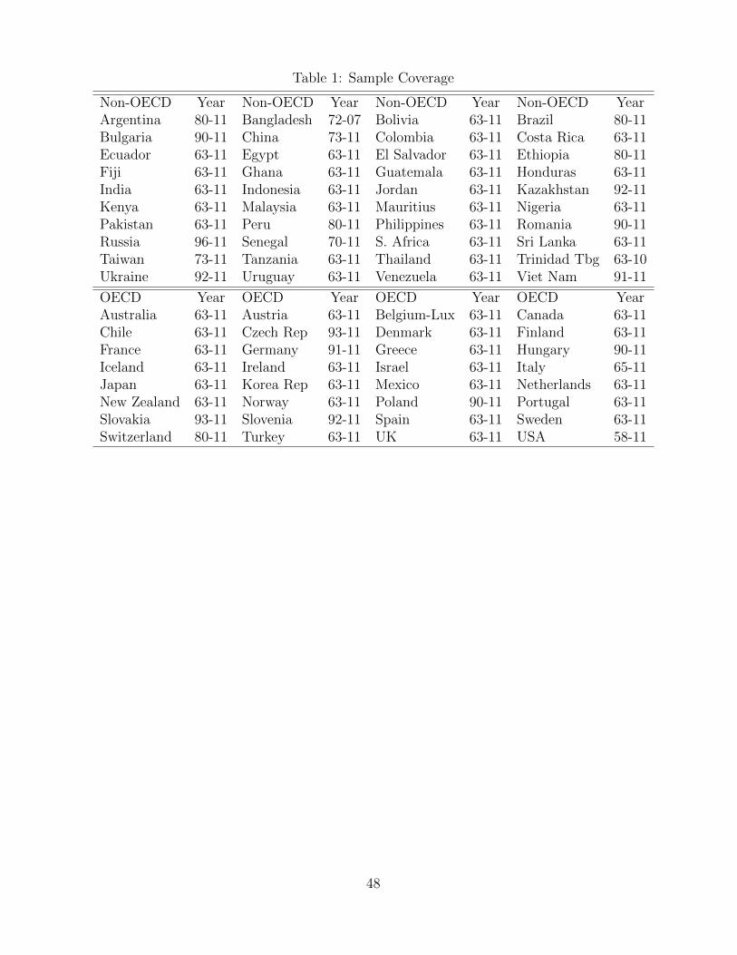
Table 1: Sample Coverage
Non-OECD Year Non-OECD Year Non-OECD Year Non-OECD YearArgentina 80-11 Bangladesh 72-07 Bolivia 63-11 Brazil 80-11Bulgaria 90-11 China 73-11 Colombia 63-11 Costa Rica 63-11Ecuador 63-11 Egypt 63-11 El Salvador 63-11 Ethiopia 80-11Fiji 63-11 Ghana 63-11 Guatemala 63-11 Honduras 63-11India 63-11 Indonesia 63-11 Jordan 63-11 Kazakhstan 92-11Kenya 63-11 Malaysia 63-11 Mauritius 63-11 Nigeria 63-11Pakistan 63-11 Peru 80-11 Philippines 63-11 Romania 90-11Russia 96-11 Senegal 70-11 S. Africa 63-11 Sri Lanka 63-11Taiwan 73-11 Tanzania 63-11 Thailand 63-11 Trinidad Tbg 63-10Ukraine 92-11 Uruguay 63-11 Venezuela 63-11 Viet Nam 91-11
OECD Year OECD Year OECD Year OECD YearAustralia 63-11 Austria 63-11 Belgium-Lux 63-11 Canada 63-11Chile 63-11 Czech Rep 93-11 Denmark 63-11 Finland 63-11France 63-11 Germany 91-11 Greece 63-11 Hungary 90-11Iceland 63-11 Ireland 63-11 Israel 63-11 Italy 65-11Japan 63-11 Korea Rep 63-11 Mexico 63-11 Netherlands 63-11New Zealand 63-11 Norway 63-11 Poland 90-11 Portugal 63-11Slovakia 93-11 Slovenia 92-11 Spain 63-11 Sweden 63-11Switzerland 80-11 Turkey 63-11 UK 63-11 USA 58-11
48

Table 2: Tradeable Sectors
ISIC (Rev. 3) Tradeable Sector15-16 Food products and beverages, tobacco products17 Textiles18-19 Wearing apparel, leather, luggage, footwear20 Wood products except furniture, straw and plaiting materials21 Paper and paper products22 Publishing, printing and reproduction of recorded media23 Coke, refined petroleum products and nuclear fuel24 Chemicals and chemical products25 Rubber and plastic products26 Other non-metallic mineral products27 Basic metals28 Fabricated metal products, except machinery and equipment29-30 Office, accounting and computing machinery, other machinery31-32 Electrical machinery, communication equipment33 Medical, precision and optical instruments, watches and clocks34-35 Transport equipment36 Furniture, other manufacturing
49

Table 3: Construction of Variables and Data Sources
Variables/Parameters Data Source & Construction MethodBilateral trade share πinn′,t UN Comtrade & UNIDO INDSTAT2
Trade deficit Dn,t UN ComtradeLabor income share γiLt UNIDO INDSTAT2, (wage bill)/(sectoral output)Capital income share γiKt UNIDO INDSTAT2, (value-added − wage bill)/(sectoral output)
Input-output coefficients γii′
n,t BEA 1997 I-O accounts (grouped into 2-digit ISIC Rev.3); WIOD
Labor supply Ln,t Penn World TableCapital stock Kn,t Penn World TableWage rate wn,t Penn World Table, (labor income)/(employment count)Rental rate rn,t Penn World Table, (total income - labor income)/(capital)Saving rate sn,t Penn World Table, implied by capital series and depreciation rate
Non-tradeable price P I+1n,t ICP, interpolate and extrapolate for non-survey years
Tradable exp share φn OECD national accounts, (fitting for non-OECD countries)Trade elasticity θi =4 (Levchenko and Zhang, 2015); =8.28 (Eaton and Kortum, 2002)Elasticity of subst. in consumption 1
1−κ 2 (Levchenko and Zhang, 2015); 1 (Caliendo and Parro, 2014)
Elasticity of subst. in production σi 2Tradeable consumption share ωin Levchenko and Zhang (2015)US sectoral TFP NBER-CES manufacturing industry databaseOther country variables Penn World TableOther bilateral variables CEPII gravity datasetSectoral TFP KLEMS database (EU-, Asia, World- KLEMS)
50

Table 4: Goodness of Fit: Baseline
Period Data Mean Model Mean Data Median Model Median Corr.
Panel I: Production Variables
Real GDP per capita (2005 US $)1990-1995 11371 12278 8162 7170 0.851996-2000 13207 14237 9659 6905 0.782001-2005 14906 14212 9433 7575 0.872006-2010 17272 28313 12827 14680 0.85
Wage (2005 US $)1990-1995 6231 4764 4660 3540 0.901996-2000 6504 5132 4963 4061 0.882001-2005 6685 5056 4775 4177 0.912006-2010 6944 6498 4932 5115 0.81
Rent1990-1995 0.18 0.18 0.16 0.18 0.351996-2000 0.19 0.22 0.16 0.21 0.422001-2005 0.19 0.16 0.16 0.10 0.532006-2010 0.20 0.20 0.17 0.14 0.53
Panel II: Trade Variables
Bilateral Trade Share1990-1995 0.0056 0.0077 3.6e-6 0 0.581996-2000 0.0062 0.0083 2.6e-5 7.3e-7 0.562001-2005 0.0069 0.0079 1.1e-4 1.7e-6 0.382006-2010 0.0074 0.0080 1.6e-4 3.0e-8 0.33
Domestic Absorption Share1990-1995 0.60 0.41 0.66 0.35 0.701996-2000 0.55 0.41 0.59 0.32 0.382001-2005 0.50 0.44 0.54 0.36 0.152006-2010 0.47 0.43 0.50 0.34 -0.02
Note: The baseline analysis includes 72 countries and 4 periods. Calibrationis targeted to Real GDP per capita across countries.
51

Table 5: Unconditional Convergence: Model versus Data
(1) (2) (3) (4) (5) (6)
ln(RCA) ln(TFP) Trade Share ln(RCA) ln(TFP) Trade Share
Actual Data (20-year) Actual Data (5-year)
Initial Value -0.40*** -0.25*** -0.15*** -0.20*** -0.16*** -0.04***Exporter FE Yes Yes Yes Yes Yes YesImporter FE Yes YesIndustry FE Yes Yes Yes Yes Yes Yes
Obs. 1005 995 83,468 3,549 3,185 250,189
Simulated Data (20-year) Simulated Data (5-year)
Initial Value -0.31*** -0.37*** -0.23*** -0.22*** -0.07*** -0.08***Exporter FE Yes Yes Yes Yes Yes YesImporter FE Yes YesIndustry FE Yes Yes Yes Yes Yes Yes
Obs. 1,193 1126 83,383 3,148 3,492 249,709
52

Table 6: Transition Probability: Model versus Data
Actual Data Simulated Data
2010 Rank 2010 Rank1-4 5-8 9-12 13-17 1-4 5-8 9-12 13-17
1990
Ran
k 1-4 0.65 0.25 0.06 0.04 0.53 0.27 0.09 0.115-8 0.20 0.43 0.29 0.08 0.28 0.31 0.28 0.139-12 0.11 0.19 0.41 0.29 0.11 0.29 0.35 0.2513-17 0.04 0.09 0.19 0.67 0.06 0.10 0.23 0.61
53

Table 7: Key Player: Country
Simple Average (%) Weighted Average (%)
Rank Direct Influence Aggregate Influence Direct Influence Aggregate Influence1990-1995
1 USA 10.13 Japan 21.69 Japan 21.59 Japan 25.812 Japan 8.60 USA 12.33 USA 18.41 USA 13.323 Germany 7.69 Germany 7.89 Germany 8.33 Germany 7.614 Italy 5.02 Italy 4.64 France 4.43 Italy 4.245 UK 4.99 France 4.26 UK 4.10 France 4.06
Brazil 2.06 Brazil 1.31 Brazil 1.75 Brazil 1.18India 1.41 India 0.64 India 0.85 India 0.55China 2.06 China 1.48 China 2.70 China 1.47S. Africa 1.07 S. Africa 0.50 S. Africa 0.52 S. Africa 0.41
1995-2000
1 USA 10.53 Japan 21.29 USA 19.51 Japan 23.922 Japan 7.42 USA 13.16 Japan 17.48 USA 14.393 Germany 6.81 Germany 6.55 Germany 6.81 Germany 6.314 Italy 6.28 Italy 6.40 Italy 5.37 Italy 5.925 UK 5.25 France 4.65 France 4.98 France 4.45
Brazil 1.74 Brazil 0.81 Brazil 1.48 Brazil 0.75Russia 0.75 Russia 0.38 Russia 0.46 Russia 0.34India 1.71 India 0.94 India 1.14 India 0.82China 2.72 China 2.40 China 3.52 China 2.42S. Africa 1.09 S. Africa 0.44 S. Africa 0.50 S. Africa 0.35
2000-2005
1 USA 9.77 Japan 19.85 USA 17.36 Japan 21.702 Japan 6.75 USA 11.29 Japan 14.70 USA 12.383 Germany 6.39 Germany 6.69 Germany 6.94 Germany 6.664 Italy 5.89 Italy 6.30 Italy 5.51 Italy 6.045 France 4.99 Korea 5.77 France 5.39 Korea 5.88
Brazil 1.93 Brazil 0.93 Brazil 1.47 Brazil 0.88Russia 0.98 Russia 0.49 Russia 0.68 Russia 0.45India 1.91 India 1.04 India 1.34 India 0.96China 4.03 China 4.21 China 5.88 China 4.40S. Africa 1.20 S. Africa 0.52 S. Africa 0.66 S. Africa 0.45
Note: Calculation of influence indices is carried out under parameters obtained frombaseline calibration and actual trade and production data. Russia is missing in 1990-1995 because there is no trade data for Russia prior to 1995 to obtain industry-levelTFP estimates. Each country’s contribution to global technology diffusion is expressedin percentage points.
54

Table 8: Key Player: Country-Industry
Simple Average (%) Weighted Average (%)
Rank Direct Influence Aggregate Influence Direct Influence Aggregate Influence1990-1995
1 Japan Electronics Japan Electronics Japan Electronics Japan Electronics2 USA Measurement Japan Fab. Metals Japan Vehicles Japan Fab. metals3 USA Chemical USA Measurement USA Chemical USA Chemical4 Germany Chemical USA Chemical Japan Machinery USA Measurement5 USA Electronics USA Electronics USA Food USA Electronics6 Japan Vehicles Japan Chemical Japan Fab. Metals Japan Chemical7 UK Chemical Germany Chemical USA Vehicles Taiwan Machinery8 Japan Machinery Taiwan Machinery Japan Chemical Japan Machinery9 Japan Chemical Taiwan Electronics USA Electronics Taiwan Electronics10 Germany Measurement Japan Machinery Taiwan Machinery Germany Chemical
1995-2000
1 Japan Electronics Japan Electronics Japan Electronics Japan Electronics2 USA Electronics USA Electronics USA Electronics USA Electronics3 USA Measurement Taiwan Electronics USA Chemical Taiwan Electronics4 USA Chemical Taiwan Machinery Japan Machinery Taiwan Machinery5 Germany Electronics Germany Electronics USA Food Germany Electronics6 Italy Fab. Metals Korea Electronics Taiwan Machinery Japan Fab. Metals7 France Electronics Italy Electronics USA Vehicles Korea Electronics8 USA Machinery Japan Fab. Metals Japan Vehicles Japan Machinery9 Italy Electronics France Electronics USA Machinery Italy Electronics10 Germany Chemical Italy Fab. Metals USA Fab. Metals Italy Fab. Metals
2000-2005
1 USA Electronics Japan Electronics Japan Electronics Japan Electronics2 Japan Electronics USA Electronics USA Electronics USA Electronics3 Germany Electronics Korea Electronics USA Chemical Korea Electronics4 Korea Electronics Germany Electronics USA Food Germany Electronics5 USA Measurement China Electronics Japan Vehicles China Electronics6 USA Chemical France Electronics Japan Machinery France Electronics7 France Electronics Taiwan Electronics USA Vehicles Taiwan Electronics8 China Electronics Italy Electronics Korea Electronics Italy Electronics9 Italy Electronics Finland Electronics USA Machinery Finland Electronics10 Italy Fab. Metals Italy Fab. Metals China Electronics Italy Fab. Metals
Note: Calculation of influence indices is carried out under parameters obtained from baseline calibration and actualtrade and production data. Each country’s contribution to global technology diffusion is expressed in percentagepoints.
55


