

Speeding Up the Convergence of Online Heuristic Search
and
Scaling Up Offline Heuristic Search
A ThesisPresented to
The Academic Faculty
by
David A. Furcy
In Partial Fulfillmentof the Requirements for the Degree
Doctor of Philosophy in theCollege of Computing
Georgia Institute of TechnologyDecember 2004

Speeding Up the Convergence of Online Heuristic Search
and
Scaling Up Offline Heuristic Search
Approved by:
Sven Koenig, Advisor
Ron Ferguson
Ashok Goel
Robert Holte(University of Alberta)
Ashwin Ram
Date Approved: 11/19/2004

ACKNOWLEDGEMENT
I would like to thank my advisor, Sven Koenig, for his help with this research. I thank my committee
members for their time and guidance. In particular, it has been a great pleasure to collaborate with
Rob Holte. I am grateful to him, Jonathan Schaeffer and everybody at the University of Alberta for
their warm welcome during my stay in Edmonton. I also enjoyed our joint work with Ariel Felner.
Over the years, I have benefited from the help of many people. Rich Korf was always willing
to share his source code and he provided me with Thorpe’s thesis, while Stefan Edelkamp was
the one who first introduced me to Thorpe’s work. Vadim Bulitko and I talked a lot about real-
time search, and he was kind enough to read drafts of some of these chapters. Rong Zhou and
Matthew McNaughton helped me get acquainted with the MSA domain. I have also had fruitful
discussions with several search experts including Blai Bonet, Hector Geffner, Eric Hansen, Istvan
Hernadvolgyi, and Wheeler Ruml. At Georgia Tech, I enjoyed the company and help of Jim Davies,
Maxim Likhachev, Yaxin Liu, Patrawadee Prasangsit, and Alex Stoychev.
Last but not least, I am immensely grateful for the love and support of my wife, Elizabeth, and
for little Abigail, who kept me awake during the last two weeks of writing and energized me for the
last stretch.
iii

TABLE OF CONTENTS
ACKNOWLEDGEMENT . . . . . . . . . . . . . . . . . . . . . . . . . . . . . . . . . . . iii
LIST OF TABLES . . . . . . . . . . . . . . . . . . . . . . . . . . . . . . . . . . . . . . ix
LIST OF FIGURES . . . . . . . . . . . . . . . . . . . . . . . . . . . . . . . . . . . . . . xi
SUMMARY . . . . . . . . . . . . . . . . . . . . . . . . . . . . . . . . . . . . . . . . . . xv
CHAPTER I OVERVIEW OF THE DISSERTATION . . . . . . . . . . . . . . . . . 1
1.1 Introduction . . . . . . . . . . . . . . . . . . . . . . . . . . . . . . . . . . . . . 1
1.2 The shortest-path problem . . . . . . . . . . . . . . . . . . . . . . . . . . . . . . 4
1.2.1 Problem statement . . . . . . . . . . . . . . . . . . . . . . . . . . . . . . 5
1.3 Structure of the dissertation . . . . . . . . . . . . . . . . . . . . . . . . . . . . . 5
1.4 Overview of our contributions to real-time search . . . . . . . . . . . . . . . . . 7
1.5 Overview of our contributions to offline search . . . . . . . . . . . . . . . . . . . 10
1.5.1 Our contributions to greedy best-first search . . . . . . . . . . . . . . . . 11
1.5.2 Our contributions to beam search . . . . . . . . . . . . . . . . . . . . . . 12
1.5.3 Summary of empirical results . . . . . . . . . . . . . . . . . . . . . . . . 13
1.5.4 Algorithm selection . . . . . . . . . . . . . . . . . . . . . . . . . . . . . 15
1.5.5 ABULB: Anytime variants of BULB . . . . . . . . . . . . . . . . . . . . 16
1.5.6 Application of ABULB to the multiple sequence alignment problem . . . 17
CHAPTER II SPEEDING UP THE CONVERGENCE OF REAL-TIME SEARCH . 18
2.1 Introduction . . . . . . . . . . . . . . . . . . . . . . . . . . . . . . . . . . . . . 18
2.2 Definitions and assumptions . . . . . . . . . . . . . . . . . . . . . . . . . . . . . 20
2.3 Learning Real-Time A* (LRTA*) . . . . . . . . . . . . . . . . . . . . . . . . . . 21
2.4 Motivation for our new action-selection rule . . . . . . . . . . . . . . . . . . . . 22
2.5 Breaking ties in favor of smaller f-values . . . . . . . . . . . . . . . . . . . . . . 25
2.6 FALCONS: Selecting actions that minimize f-values . . . . . . . . . . . . . . . . 26
2.6.1 FALCONS: A naive approach . . . . . . . . . . . . . . . . . . . . . . . 26
2.6.2 FALCONS: The final version . . . . . . . . . . . . . . . . . . . . . . . 29
2.7 Experimental results . . . . . . . . . . . . . . . . . . . . . . . . . . . . . . . . 31
2.7.1 Domains and heuristics . . . . . . . . . . . . . . . . . . . . . . . . . . . 31
iv

2.7.2 Performance measures . . . . . . . . . . . . . . . . . . . . . . . . . . . 33
2.7.3 Empirical setup . . . . . . . . . . . . . . . . . . . . . . . . . . . . . . . 35
2.7.4 Results . . . . . . . . . . . . . . . . . . . . . . . . . . . . . . . . . . . . 36
2.8 Related work . . . . . . . . . . . . . . . . . . . . . . . . . . . . . . . . . . . . . 39
2.9 Future work . . . . . . . . . . . . . . . . . . . . . . . . . . . . . . . . . . . . . 41
2.10 Contributions . . . . . . . . . . . . . . . . . . . . . . . . . . . . . . . . . . . . 42
CHAPTER III SCALING UP WA* WITH COMMITMENT AND DIVERSITY . . . 43
3.1 Introduction . . . . . . . . . . . . . . . . . . . . . . . . . . . . . . . . . . . . . 43
3.2 The WA* algorithm . . . . . . . . . . . . . . . . . . . . . . . . . . . . . . . . . 44
3.3 The KWA* algorithm: Introducing diversity in WA* . . . . . . . . . . . . . . . . 46
3.4 The MSC-WA* algorithm: Introducing commitment in WA* . . . . . . . . . . . 48
3.5 The MSC-KWA* algorithm: Combining diversity and commitment . . . . . . . . 51
3.5.1 Comparing the behaviors of KWA* and MSC-WA* . . . . . . . . . . . . 52
3.5.2 The MSC-KWA* algorithm . . . . . . . . . . . . . . . . . . . . . . . . . 55
3.6 Empirical evaluation . . . . . . . . . . . . . . . . . . . . . . . . . . . . . . . . . 57
3.6.1 The�
-Puzzle domain . . . . . . . . . . . . . . . . . . . . . . . . . . . . 57
3.6.2 The 4-peg Towers of Hanoi domain . . . . . . . . . . . . . . . . . . . . . 59
3.6.3 The Rubik’s Cube domain . . . . . . . . . . . . . . . . . . . . . . . . . 61
3.6.4 Empirical setup . . . . . . . . . . . . . . . . . . . . . . . . . . . . . . . 62
3.6.5 Empirical results in the�
-Puzzle domain . . . . . . . . . . . . . . . . . 64
3.6.5.1 Empirical evaluation of WA* in the�
-Puzzle . . . . . . . . . . 64
3.6.5.2 Empirical evaluation of KWA* in the�
-Puzzle . . . . . . . . . 66
3.6.5.3 Empirical evaluation of MSC-WA* in the�
-Puzzle . . . . . . 71
3.6.5.4 Empirical evaluation of MSC-KWA* in the�
-Puzzle . . . . . 75
3.6.5.5 Empirical comparison of WA*, KWA*, MSC-WA*, and MSC-KWA* in the
�-Puzzle . . . . . . . . . . . . . . . . . . . . . 80
3.6.6 Empirical results in the 4-peg Towers of Hanoi domain . . . . . . . . . . 80
3.6.7 Empirical results in the Rubik’s Cube domain . . . . . . . . . . . . . . . 82
3.7 Related work . . . . . . . . . . . . . . . . . . . . . . . . . . . . . . . . . . . . . 83
3.7.1 Multi-state commitment applied to RTA* search . . . . . . . . . . . . . . 84
3.7.1.1 The RTA* algorithm . . . . . . . . . . . . . . . . . . . . . . . 84
v

3.7.1.2 The MSC-RTA* algorithm . . . . . . . . . . . . . . . . . . . . 85
3.7.2 Beam search . . . . . . . . . . . . . . . . . . . . . . . . . . . . . . . . . 87
3.8 Future work . . . . . . . . . . . . . . . . . . . . . . . . . . . . . . . . . . . . . 88
3.8.1 Domain-dependent behaviors of MSC-KWA* . . . . . . . . . . . . . . . 88
3.8.2 MSC-KWA* versus beam search . . . . . . . . . . . . . . . . . . . . . . 89
3.8.2.1 Preliminary study of MSC-KWA* with ��������� in the�
-Puzzle . . . . . . . . . . . . . . . . . . . . . . . . . . . . . . 89
3.8.3 Introducing diversity in MSC-RTA* . . . . . . . . . . . . . . . . . . . . 92
3.8.3.1 The MSC-KRTA* algorithm . . . . . . . . . . . . . . . . . . . 92
3.9 Conclusions . . . . . . . . . . . . . . . . . . . . . . . . . . . . . . . . . . . . . 95
CHAPTER IV LIMITED DISCREPANCY BEAM SEARCH . . . . . . . . . . . . . . 97
4.1 Introduction . . . . . . . . . . . . . . . . . . . . . . . . . . . . . . . . . . . . . 97
4.2 Beam search . . . . . . . . . . . . . . . . . . . . . . . . . . . . . . . . . . . . . 99
4.2.1 The beam search algorithm . . . . . . . . . . . . . . . . . . . . . . . . . 100
4.2.2 Motivation for backtracking beam search . . . . . . . . . . . . . . . . . . 104
4.3 Backtracking beam search . . . . . . . . . . . . . . . . . . . . . . . . . . . . . . 106
4.3.1 The depth-first beam search (DB) algorithm . . . . . . . . . . . . . . . . 106
4.3.2 Limited discrepancy search . . . . . . . . . . . . . . . . . . . . . . . . . 110
4.3.2.1 Original limited discrepancy search . . . . . . . . . . . . . . . 110
4.3.2.2 Generalized limited discrepancy search . . . . . . . . . . . . . 113
4.3.3 Beam search using limited discrepancy backtracking (BULB) . . . . . . . 116
4.3.4 Properties of the BULB algorithm . . . . . . . . . . . . . . . . . . . . . 118
4.3.4.1 BULB is a memory-bounded algorithm . . . . . . . . . . . . . 118
4.3.4.2 BULB generalizes both limited discrepancy search and breadth-first search . . . . . . . . . . . . . . . . . . . . . . . . . . . . 118
4.3.4.3 BULB is a complete algorithm . . . . . . . . . . . . . . . . . . 119
4.3.4.4 BULB eliminates all cycles and some transpositions . . . . . . 120
4.4 Empirical evaluation . . . . . . . . . . . . . . . . . . . . . . . . . . . . . . . . . 121
4.4.1 Empirical evaluation in the�
-Puzzle domain . . . . . . . . . . . . . . . 121
4.4.1.1 Evaluation of beam search in the�
-Puzzle . . . . . . . . . . . 121
4.4.1.2 Evaluation of BULB in the�
-Puzzle . . . . . . . . . . . . . . 123
4.4.1.3 Comparison with variants of multi-state commitment search . . 124
vi

4.4.1.4 BULB scales up to even larger puzzles . . . . . . . . . . . . . 124
4.4.2 Empirical evaluation in the Towers of Hanoi domain . . . . . . . . . . . . 127
4.4.3 Empirical evaluation in the Rubik’s Cube domain . . . . . . . . . . . . . 130
4.5 Related work . . . . . . . . . . . . . . . . . . . . . . . . . . . . . . . . . . . . . 133
4.5.1 Band search . . . . . . . . . . . . . . . . . . . . . . . . . . . . . . . . . 133
4.5.2 Diversity beam search . . . . . . . . . . . . . . . . . . . . . . . . . . . . 136
4.5.3 Complete anytime beam search . . . . . . . . . . . . . . . . . . . . . . . 136
4.5.4 Variants of discrepancy search . . . . . . . . . . . . . . . . . . . . . . . 137
4.5.5 Divide-and-conquer beam search . . . . . . . . . . . . . . . . . . . . . . 139
4.6 Future work . . . . . . . . . . . . . . . . . . . . . . . . . . . . . . . . . . . . . 140
4.7 Conclusion . . . . . . . . . . . . . . . . . . . . . . . . . . . . . . . . . . . . . . 141
CHAPTER V ANYTIME HEURISTIC SEARCH . . . . . . . . . . . . . . . . . . . . 143
5.1 Introduction . . . . . . . . . . . . . . . . . . . . . . . . . . . . . . . . . . . . . 143
5.2 ITSA*: Application of local search to the shortest-path problem . . . . . . . . . . 144
5.2.1 Motivation . . . . . . . . . . . . . . . . . . . . . . . . . . . . . . . . . . 145
5.2.2 A neighborhood structure based on path proximity . . . . . . . . . . . . . 147
5.2.3 The ITSA* algorithm . . . . . . . . . . . . . . . . . . . . . . . . . . . . 149
5.2.4 Empirical evaluation of ITSA* . . . . . . . . . . . . . . . . . . . . . . . 150
5.3 ABULB: Anytime BULB . . . . . . . . . . . . . . . . . . . . . . . . . . . . . . 153
5.3.1 BULB + ITSA*: Local optimization of BULB’s solutions . . . . . . . . . 153
5.3.2 ABULB 1.0: Continuous execution of BULB with a constant value . . 156
5.3.3 ABULB 2.0: Restart of BULB with varying values . . . . . . . . . . . 158
5.3.4 ABULB + ITSA*: Local optimization of ABULB’s solutions . . . . . . . 160
5.3.5 Empirical evaluation of ABULB . . . . . . . . . . . . . . . . . . . . . . 161
5.4 Related work . . . . . . . . . . . . . . . . . . . . . . . . . . . . . . . . . . . . . 166
5.4.1 Anytime heuristic search . . . . . . . . . . . . . . . . . . . . . . . . . . 166
5.4.2 Local search . . . . . . . . . . . . . . . . . . . . . . . . . . . . . . . . . 168
5.5 Conclusion . . . . . . . . . . . . . . . . . . . . . . . . . . . . . . . . . . . . . . 168
CHAPTER VI THE MULTIPLE SEQUENCE ALIGNMENT PROBLEM . . . . . . 171
6.1 Introduction . . . . . . . . . . . . . . . . . . . . . . . . . . . . . . . . . . . . . 171
6.2 Sequence alignment . . . . . . . . . . . . . . . . . . . . . . . . . . . . . . . . . 172
vii

6.3 Evaluating alignments . . . . . . . . . . . . . . . . . . . . . . . . . . . . . . . . 173
6.4 Pairwise sequence alignment . . . . . . . . . . . . . . . . . . . . . . . . . . . . 175
6.5 Multiple sequence alignment (MSA) . . . . . . . . . . . . . . . . . . . . . . . . 178
6.6 The MSA problem as a shortest-path problem . . . . . . . . . . . . . . . . . . . 181
6.7 Solving the MSA problem with search algorithms . . . . . . . . . . . . . . . . . 182
6.7.1 An admissible heuristic function for the MSA problem . . . . . . . . . . 184
6.7.2 Solving the MSA problem with existing variants of A* . . . . . . . . . . 187
6.8 Solving the MSA problem with ABULB . . . . . . . . . . . . . . . . . . . . . . 189
6.8.1 Adapting ABULB to the MSA problem . . . . . . . . . . . . . . . . . . 189
6.8.2 Empirical evaluation . . . . . . . . . . . . . . . . . . . . . . . . . . . . 191
6.8.2.1 Empirical setup . . . . . . . . . . . . . . . . . . . . . . . . . . 191
6.8.2.2 Empirical results . . . . . . . . . . . . . . . . . . . . . . . . . 192
6.9 Conclusion . . . . . . . . . . . . . . . . . . . . . . . . . . . . . . . . . . . . . . 196
CHAPTER VII CONCLUSIONS AND FUTURE WORK IN OFFLINE SEARCH . . . 198
7.1 Our contributions to offline search . . . . . . . . . . . . . . . . . . . . . . . . . 198
7.1.1 Our contributions to one-shot search . . . . . . . . . . . . . . . . . . . . 198
7.1.2 Our contributions to anytime search . . . . . . . . . . . . . . . . . . . . 200
7.2 Lessons learned and future work . . . . . . . . . . . . . . . . . . . . . . . . . . 201
7.2.1 Generalization of MSC-KWA* and beam search . . . . . . . . . . . . . . 201
7.2.2 Application of neighborhood search to the shortest-path problem . . . . . 202
7.2.3 Domain-specific extensions . . . . . . . . . . . . . . . . . . . . . . . . 204
APPENDIX A — FORMAL PROOFS FOR FALCONS . . . . . . . . . . . . . . . . 206
APPENDIX B — EMPIRICAL EVALUATION OF VARIANTS OF WA* IN THE�
-PUZZLE . . . . . . . . . . . . . . . . . . . . . . . . . . . . . . . . . . . . . . . . . 222
REFERENCES . . . . . . . . . . . . . . . . . . . . . . . . . . . . . . . . . . . . . . . . . 247
viii

LIST OF TABLES
Table 1 Speedup of FALCONS over LRTA* . . . . . . . . . . . . . . . . . . . . . . . . 9
Table 2 Scaling behavior in our three benchmark domains . . . . . . . . . . . . . . . . . 14
Table 3 Travel cost to convergence with different tie-breaking rules . . . . . . . . . . . . 27
Table 4 Travel cost to convergence with different action-selection rules . . . . . . . . . . 32
Table 5 Trials to convergence with different action-selection rules . . . . . . . . . . . . 36
Table 6 Travel cost of the first trial with different action-selection rules . . . . . . . . . . 37
Table 7 Travel cost to convergence with different action-selection rules, and with or with-out g updates for FALCONS . . . . . . . . . . . . . . . . . . . . . . . . . . . . 38
Table 8 Comparison of WA*, KWA*, and MSC-WA* in the�
-Puzzle . . . . . . . . . . 54
Table 9 Performance of WA* in the 35-Puzzle with varying . . . . . . . . . . . . . . 67
Table 10 Performance of KWA* in the 48-Puzzle when solving at least two thirds of theinstances . . . . . . . . . . . . . . . . . . . . . . . . . . . . . . . . . . . . . . 74
Table 11 Performance of MSC-WA* in the 48-Puzzle when solving at least two thirds ofthe instances . . . . . . . . . . . . . . . . . . . . . . . . . . . . . . . . . . . . 75
Table 12 Comparison of WA*, KWA*, MSC-WA*, and MSC-KWA* in the�
-Puzzle . . 81
Table 13 Best performance of all algorithms in the Towers of Hanoi domain (mem-ory = 1 million nodes) . . . . . . . . . . . . . . . . . . . . . . . . . . . . . . . 81
Table 14 Performance of MSC-KWA* in the Towers of Hanoi domain when solving allinstances (memory = 1 million nodes) . . . . . . . . . . . . . . . . . . . . . . . 82
Table 15 Best performance of all algorithms in the Rubik’s Cube domain (memory = 2million nodes) . . . . . . . . . . . . . . . . . . . . . . . . . . . . . . . . . . . 83
Table 16 Performance of MSC-KWA* with varying � and � in the 48-Puzzle when solv-ing all instances with an average solution cost of less than 10,000 . . . . . . . . 90
Table 17 Performance of beam search in the 48-Puzzle . . . . . . . . . . . . . . . . . . . 105
Table 18 A taxonomy of beam search methods . . . . . . . . . . . . . . . . . . . . . . . 118
Table 19 Performance of beam search in the Towers of Hanoi domain (memory = 1 millionnodes) . . . . . . . . . . . . . . . . . . . . . . . . . . . . . . . . . . . . . . . . 128
Table 20 Performance of beam search in the Rubik’s Cube domain (memory = 1 millionnodes) . . . . . . . . . . . . . . . . . . . . . . . . . . . . . . . . . . . . . . . . 131
Table 21 Performance of BULB in the Rubik’s Cube domain averaged over 1,000 randominstances (memory = 1 million nodes) . . . . . . . . . . . . . . . . . . . . . . . 131
Table 22 Performance of one-step ITSA* on paths found by BULB in the 48-Puzzle (with6 million nodes in memory) . . . . . . . . . . . . . . . . . . . . . . . . . . . . 150
ix
Table 23 Performance of one-step ITSA* on paths found by BULB in the Rubik’s Cube(with 3 million nodes in memory) . . . . . . . . . . . . . . . . . . . . . . . . . 151
Table 24 Performance of multi-step ITSA* on paths found by BULB in the 48-Puzzle (with6 million nodes in memory) . . . . . . . . . . . . . . . . . . . . . . . . . . . . 152
Table 25 Performance of multi-step ITSA* on paths found by BULB in the Rubik’s Cube(with 3 million nodes in memory) . . . . . . . . . . . . . . . . . . . . . . . . . 152
Table 26 Versions of Anytime BULB (ABULB) . . . . . . . . . . . . . . . . . . . . . . 161
x

LIST OF FIGURES
Figure 1 A taxonomy of heuristic search algorithms (with our contributions in red) . . . . 6
Figure 2 Lineage of our new offline heuristic search algorithms . . . . . . . . . . . . . . 10
Figure 3 The LRTA* algorithm . . . . . . . . . . . . . . . . . . . . . . . . . . . . . . . 21
Figure 4 Two action-selection rules for real-time search. Curves represent iso-contours fora) cost-to-goal estimates and b) f-values. . . . . . . . . . . . . . . . . . . . . . 24
Figure 5 The TB-LRTA* algorithm . . . . . . . . . . . . . . . . . . . . . . . . . . . . . 26
Figure 6 Naive FALCONS (initial, non-functional version) . . . . . . . . . . . . . . . . . 28
Figure 7 Naive FALCONS cycles forever (Each circle represents a state with its g-value/h-value) . . . . . . . . . . . . . . . . . . . . . . . . . . . . . . . . . . . . . . . 28
Figure 8 Naive FALCONS converges to a sub-optimal path (Each circle represents a statewith its g-value/h-value) . . . . . . . . . . . . . . . . . . . . . . . . . . . . . . 29
Figure 9 The FALCONS algorithm (final version) . . . . . . . . . . . . . . . . . . . . . 29
Figure 10 Roadmap for this research . . . . . . . . . . . . . . . . . . . . . . . . . . . . . 44
Figure 11 The WA* algorithm . . . . . . . . . . . . . . . . . . . . . . . . . . . . . . . . 45
Figure 12 The KWA* algorithm . . . . . . . . . . . . . . . . . . . . . . . . . . . . . . . 48
Figure 13 The MSC-WA* algorithm . . . . . . . . . . . . . . . . . . . . . . . . . . . . . 50
Figure 14 Performance comparison: WA*, KWA*, and MSC-WA* in the�
-Puzzle . . . . 53
Figure 15 The MSC-KWA* algorithm . . . . . . . . . . . . . . . . . . . . . . . . . . . . 56
Figure 16 The 15-Puzzle . . . . . . . . . . . . . . . . . . . . . . . . . . . . . . . . . . . 57
Figure 17 The 4-peg Towers of Hanoi . . . . . . . . . . . . . . . . . . . . . . . . . . . . 59
Figure 18 The Rubik’s Cube . . . . . . . . . . . . . . . . . . . . . . . . . . . . . . . . . 61
Figure 19 Performance of WA* in the�
-Puzzle with varying . . . . . . . . . . . . . . 65
Figure 20 Performance of KWA* in the 35-Puzzle with varying . . . . . . . . . . . . . 69
Figure 21 Performance of KWA* in the 35-Puzzle with varying � . . . . . . . . . . . . . 70
Figure 22 Performance of MSC-WA* in the 35-Puzzle with varying . . . . . . . . . . . 72
Figure 23 Performance of MSC-WA* in the 35-Puzzle with varying � . . . . . . . . . . . 73
Figure 24 Solution cost versus for MSC-KWA* ( ��� � ) in the 35-Puzzle . . . . . . . 77
Figure 25 Memory usage versus for MSC-KWA* ( ��� � ) in the 35-Puzzle . . . . . . 77
Figure 26 Solution cost versus � for MSC-KWA* ( ��� � ) in the 35-Puzzle . . . . . . . 78
Figure 27 Memory usage versus � for MSC-KWA* ( ����� ) in the 35-Puzzle . . . . . . 78
xi

Figure 28 Memory usage versus solution cost for MSC-KWA* ( ����� ) in the 35-Puzzlewith varying . . . . . . . . . . . . . . . . . . . . . . . . . . . . . . . . . . . 78
Figure 29 Performance comparison: WA*, KWA*, MSC-WA*, and MSC-KWA* in the�
-Puzzle . . . . . . . . . . . . . . . . . . . . . . . . . . . . . . . . . . . . . . . . 79
Figure 30 The RTA* algorithm . . . . . . . . . . . . . . . . . . . . . . . . . . . . . . . . 84
Figure 31 The MSC-RTA* algorithm . . . . . . . . . . . . . . . . . . . . . . . . . . . . . 86
Figure 32 Proposed evolution of RTA* . . . . . . . . . . . . . . . . . . . . . . . . . . . . 91
Figure 33 The MSC-KRTA* algorithm . . . . . . . . . . . . . . . . . . . . . . . . . . . . 93
Figure 34 Performance comparison: WA*, KWA*, MSC-WA*, MSC-KWA*, MSC-RTA*,and MSC-KRTA* in the
�-Puzzle . . . . . . . . . . . . . . . . . . . . . . . . . 94
Figure 35 Performance comparison: MSC-KWA*, MSC-RTA*, and MSC-KRTA* in the48-Puzzle . . . . . . . . . . . . . . . . . . . . . . . . . . . . . . . . . . . . . . 95
Figure 36 Roadmap for this research . . . . . . . . . . . . . . . . . . . . . . . . . . . . . 99
Figure 37 Levels of search strategies . . . . . . . . . . . . . . . . . . . . . . . . . . . . . 100
Figure 38 From breadth-first search to beam search to depth-first beam search . . . . . . . 101
Figure 39 The beam search algorithm . . . . . . . . . . . . . . . . . . . . . . . . . . . . . 103
Figure 40 The depth-first beam search (DB) algorithm . . . . . . . . . . . . . . . . . . . . 108
Figure 41 Behavior of original limited discrepancy search (LDS) on a balanced, binary tree 111
Figure 42 The original limited discrepancy search (LDS) algorithm (for balanced binary trees)112
Figure 43 The limited discrepancy search algorithm for general graphs (GLDS) . . . . . . 114
Figure 44 Behavior of GLDS on an irregular tree . . . . . . . . . . . . . . . . . . . . . . 115
Figure 45 The BULB algorithm: Beam search using limited discrepancy backtracking . . 117
Figure 46 From beam search to BULB search . . . . . . . . . . . . . . . . . . . . . . . . 119
Figure 47 Cycles and transpositions . . . . . . . . . . . . . . . . . . . . . . . . . . . . . 120
Figure 48 Performance of beam search in the�
-Puzzle with varying . . . . . . . . . . . 122
Figure 49 Performance of BULB in the 48-Puzzle with varying . . . . . . . . . . . . . 125
Figure 50 Comparing the performance of beam search and BULB with that of MSC-KWA*and MSC-KRTA* in the 48-Puzzle with varying . . . . . . . . . . . . . . . . 126
Figure 51 Performance of BULB in the 63-Puzzle with varying (memory = 4 million nodes)126
Figure 52 Performance of BULB in the 80-Puzzle with varying (memory = 3 million nodes)127
Figure 53 Performance of BULB in the Towers of Hanoi domain with varying (memory= 1 million nodes) . . . . . . . . . . . . . . . . . . . . . . . . . . . . . . . . . 129
Figure 54 Performance of beam search and BULB in the Rubik’s Cube with varying (memory = 1 million nodes) . . . . . . . . . . . . . . . . . . . . . . . . . . . . 132
xii

Figure 55 Approximation algorithms explore the search space in a less regular way thanadmissible algorithms. . . . . . . . . . . . . . . . . . . . . . . . . . . . . . . . 145
Figure 56 Solutions found (unbroken line) and missed (dashed line) by WA* with ������������ in a gridworld problem. . . . . . . . . . . . . . . . . . . . . . . . . . 146
Figure 57 Iterative tunneling defines the neighborhood of a path. . . . . . . . . . . . . . . 148
Figure 58 Building a performance profile . . . . . . . . . . . . . . . . . . . . . . . . . . . 154
Figure 59 Performance of ITSA* on solutions produced by BULB in the 48-Puzzle (with 6million nodes and B=5) . . . . . . . . . . . . . . . . . . . . . . . . . . . . . . 155
Figure 60 An average point lies above the average curve . . . . . . . . . . . . . . . . . . . 156
Figure 61 Performance of ITSA* on solutions produced by BULB in the Rubik’s Cubedomain (with 1 million nodes and B=70) . . . . . . . . . . . . . . . . . . . . . 157
Figure 62 Behavior of ABULB 1.0 . . . . . . . . . . . . . . . . . . . . . . . . . . . . . . 158
Figure 63 Behavior of ABULB 2.0 . . . . . . . . . . . . . . . . . . . . . . . . . . . . . . 159
Figure 64 ABULB + ITSA*: A neighborhood search in the space of solution paths . . . . 160
Figure 65 ABULB 1.0 versus ABULB 2.0 in the 48-Puzzle (with 6 million nodes and B=5) 162
Figure 66 ABULB 1.0 versus ABULB 2.0 in the Rubik’s Cube domain (with 1 millionnodes and B=70) . . . . . . . . . . . . . . . . . . . . . . . . . . . . . . . . . . 163
Figure 67 Combining ITSA* with ABULB 1 in the 48-Puzzle (with 6 million nodes and B=5)164
Figure 68 Combining ITSA* with ABULB 2 in the 48-Puzzle (with 6 million nodes and B=5)164
Figure 69 Combining ITSA* with ABULB 1 in the Rubik’s Cube domain (with 1 millionnodes and B=70) . . . . . . . . . . . . . . . . . . . . . . . . . . . . . . . . . . 165
Figure 70 Combining ITSA* with ABULB 2 in the Rubik’s Cube domain (with 1 millionnodes and B=70) . . . . . . . . . . . . . . . . . . . . . . . . . . . . . . . . . . 165
Figure 71 Three pairwise alignments (taken from [33]) . . . . . . . . . . . . . . . . . . . 172
Figure 72 The PAM250 substitution matrix . . . . . . . . . . . . . . . . . . . . . . . . . . 174
Figure 73 One step in the alignment of two sequences . . . . . . . . . . . . . . . . . . . . 176
Figure 74 The Needleman-Wunsch dynamic programming algorithm . . . . . . . . . . . . 177
Figure 75 Computing the optimal alignment of the two sequences in Figure 73a . . . . . . 178
Figure 76 Search tree for the 2-dimensional MSA problem in Figure 73a . . . . . . . . . . 179
Figure 77 State space for the 2-dimensional MSA problem in Figure 73a . . . . . . . . . . 180
Figure 78 A 3-dimensional MSA problem . . . . . . . . . . . . . . . . . . . . . . . . . . 180
Figure 79 Solving the MSA problem with search algorithms . . . . . . . . . . . . . . . . . 183
Figure 80 Computing the h-values for the MSA problem . . . . . . . . . . . . . . . . . . 185
Figure 81 Search space and corresponding search tree for an MSA problem with ����� �"! 190
xiii

Figure 82 MSA problems with 8 proteins . . . . . . . . . . . . . . . . . . . . . . . . . . . 193
Figure 83 MSA problems with 9 proteins . . . . . . . . . . . . . . . . . . . . . . . . . . . 194
Figure 84 MSA problems with 10 proteins . . . . . . . . . . . . . . . . . . . . . . . . . . 194
Figure 85 MSA problems with 11 proteins . . . . . . . . . . . . . . . . . . . . . . . . . . 195
Figure 86 MSA problems with 12 proteins . . . . . . . . . . . . . . . . . . . . . . . . . . 195
Figure 87 MSA problems with 13 proteins . . . . . . . . . . . . . . . . . . . . . . . . . . 196
Figure 88 The FALCONS algorithm . . . . . . . . . . . . . . . . . . . . . . . . . . . . . 207
Figure 89 Performance of KWA* in the 8-Puzzle with varying . . . . . . . . . . . . . . 223
Figure 90 Performance of KWA* in the 8-Puzzle with varying � . . . . . . . . . . . . . . 224
Figure 91 Performance of KWA* in the 15-Puzzle with varying . . . . . . . . . . . . . 225
Figure 92 Performance of KWA* in the 15-Puzzle with varying � . . . . . . . . . . . . . 226
Figure 93 Performance of KWA* in the 24-Puzzle with varying . . . . . . . . . . . . . 227
Figure 94 Performance of KWA* in the 24-Puzzle with varying � . . . . . . . . . . . . . 228
Figure 95 Performance of MSC-WA* in the 8-Puzzle with varying . . . . . . . . . . . 230
Figure 96 Performance of MSC-WA* in the 8-Puzzle with varying � . . . . . . . . . . . . 231
Figure 97 Performance of MSC-WA* in the 15-Puzzle with varying . . . . . . . . . . . 232
Figure 98 Performance of MSC-WA* in the 15-Puzzle with varying � . . . . . . . . . . . 233
Figure 99 Performance of MSC-WA* in the 24-Puzzle with varying . . . . . . . . . . . 234
Figure 100 Performance of MSC-WA* in the 24-Puzzle with varying � . . . . . . . . . . . 235
Figure 101 Performance of MSC-KWA* in the 8-Puzzle with varying . . . . . . . . . . 237
Figure 102 Performance of MSC-KWA* in the 8-Puzzle with varying � . . . . . . . . . . . 238
Figure 103 Performance of MSC-KWA* in the 15-Puzzle with varying . . . . . . . . . . 239
Figure 104 Performance of MSC-KWA* in the 15-Puzzle with varying � . . . . . . . . . . 240
Figure 105 Performance of MSC-KWA* in the 24-Puzzle with varying . . . . . . . . . . 241
Figure 106 Performance of MSC-KWA* in the 24-Puzzle with varying � . . . . . . . . . . 242
Figure 107 Performance of MSC-KWA* in the 35-Puzzle with varying . . . . . . . . . . 243
Figure 108 Performance of MSC-KWA* in the 35-Puzzle with varying � . . . . . . . . . . 244
Figure 109 Performance of MSC-KWA* in the 48-Puzzle with varying . . . . . . . . . . 245
Figure 110 Performance of MSC-KWA* in the 48-Puzzle with varying � . . . . . . . . . . 246
xiv
SUMMARY
Heuristic search algorithms are popular Artificial Intelligence methods for solving the
shortest-path problem. This research contributes new heuristic search algorithms that are either
faster or scale up to larger problems than existing algorithms. Our contributions apply to both
online and offline tasks.
For online tasks, existing real-time heuristic search algorithms learn better informed heuristic
values and sometimes eventually converge to a shortest path by repeatedly executing the action
leading to a successor state with a minimum cost-to-goal estimate. In contrast, we claim that real-
time heuristic search converges faster to a shortest path when it always selects an action leading
to a state with a minimum f-value (i.e., a minimum estimate of the cost of a shortest path from
start to goal via the state), just like in the offline A* search algorithm. We support this claim by
implementing this new non-trivial action-selection rule in FALCONS and by showing empirically
that FALCONS significantly reduces the number of actions to convergence of a state-of-the-art real-
time search algorithm.
For offline tasks, we scale up two best-first search approaches. First, a greedy variant of A*
called WA* is known 1) to consume less memory to find solutions of equal cost when it is diversified
(i.e., when it performs expansions in parallel), as in KWA*; and 2) to solve larger problems when
it is committed (i.e., when it chooses the state to expand next among a fixed-size subset of the
set of generated but unexpanded states), as in MSC-WA*. We claim that WA* solves even larger
problems when it is enhanced with both diversity and commitment. We support this claim with
our MSC-KWA* algorithm. Second, it is known that breadth-first search solves larger problems
when it prunes unpromising states, resulting in the beam search algorithm. We claim that beam
search quickly solves even larger problems when it is enhanced with backtracking based on limited
discrepancy search. We support this claim with our BULB algorithm. We demonstrate the improved
scaling of MSC-KWA* and BULB empirically in three standard benchmark domains. Finally, we
apply anytime variants of BULB to the multiple sequence alignment problem in biology.
xv

CHAPTER I
OVERVIEW OF THE DISSERTATION
1.1 Introduction
The most popular methods for solving the shortest-path problem in Artificial Intelligence (AI) are
heuristic search algorithms. In particular, best-first search algorithms always expand next a node
with the smallest f-value, where the f-value of a node estimates the cost of a shortest path from the
start to a goal via the node. In breadth-first (or uniform-cost) search [29], the f-value is equal to the
g-value of the node, which is the cost of the shortest path found so far from the start to the node.
In the A* algorithm [59], the f-value is the sum of the g-value and the h-value of the node, which
is an estimate of the cost of a shortest path from the node to the goal. A* and breadth-first search
are offline search algorithms since they find a complete path to the goal before they terminate. In
contrast, online (and more specifically real-time) search algorithms interleave searching for a partial
path from the current node and traversing this path in the environment. Such algorithms are useful
for tasks that have tight time constraints on each action execution. We now discuss in turn our
hypotheses pertaining to real-time and offline heuristic search.
Real-time search. Existing real-time heuristic search methods, such as LRTA* [98], repeatedly
select and execute the action leading to a successor with minimum h-value. Before each execution,
they also update the h-value of the current node so that they learn better informed h-values over
time. When the goal is reached (we say that the current trial is over), the agent is reset to the
start (and the next trial begins). Their learning component enables real-time search methods to
eventually converge to a shortest path. However, we claim that minimizing h-values is not the best
action-selection rule for fast convergence. We propose the following hypothesis:
Hypothesis 1 (Real-time search hypothesis) Real-time heuristic search converges faster to a
shortest path when it selects actions leading to nodes with a minimum estimated cost of a short-
est path going from the start through the node and to the goal.
1

In Chapter 2, we will support this hypothesis with FALCONS, a new real-time search algorithm
that converges to a shortest path with significantly fewer actions and trials than LRTA*. We will
show that the correct design of our action-selection rule in FALCONS is not trivial. Nevertheless,
Appendix A will prove that FALCONS shares the same theoretical properties as LRTA*. We will
show empirically that FALCONS converges with fewer actions and trials than LRTA* in all of our
thirteen different empirical conditions (corresponding to six standard benchmark domains with two
or more heuristic functions per domain). Convergence with fewer actions and trials means that the
overall learning time is shorter since both the total time spent executing actions and the total pre-
trial setup time are smaller. This speedup is important in domains from real-time control. The main
limitations of FALCONS are that 1) the duration of the first trial is sometimes larger because more
exploration is performed at the beginning, 2) FALCONS may not perform well in directed domains
because its action-selection rule is based exclusively on the f-value of the successor node and does
not take into account the edge cost to reach it, and 3) FALCONS only applies to deterministic
domains.
Offline search. The main drawback of both breadth-first search and A* is that they store all
generated nodes in memory. Therefore, they quickly run out of memory on large graphs. To remedy
this problem and scale up heuristic search to larger problems, one common approach is to sacrifice
solution quality (breadth-first search and A* are admissible algorithms, that is, they always find a
shortest path, provided they have enough memory). One typically reduces memory consumption by
making the search greedy (but still storing all generated nodes) or by pruning some nodes (that is,
not storing some of the generated nodes). We summarize in turn our contributions to each class of
approaches.
First, it is known that WA* makes A* search greedy by weighing the h-value more than the
g-value when adding them up to compute each f-value. WA* can solve larger problems than A*
[132, 52]. It is also known that WA* with diversity (that is, the parallel expansion of several nodes
at each iteration, like in KWA* [37]) uses less memory than WA* to find solutions of equal cost.
Furthermore, it is known that WA* with commitment (that is, the focus on a sub-set of the candidate
nodes for expansion, like in MSC-WA* [88]) scales up to larger problems than WA*. We propose
the following hypothesis:
2
Hypothesis 2 (Offline search hypothesis #1) WA* solves larger problems when it is enhanced
with both diversity and commitment.
In Chapter 3, we will support this hypothesis with MSC-KWA*, a new offline search algorithm
that can solve larger problems than WA*, KWA* and MSC-WA* in three benchmark domains. In
our empirical setup, MSC-KWA* is the only considered variant of WA* that can solve all of our
random instances in the 48-Puzzle and the 4-peg Towers of Hanoi domain. Furthermore, MSC-
KWA* solves the largest percentage of random instances in the Rubik’s Cube domain. However,
MSC-KWA* shares with WA*, MSC-WA* and KWA* the limitation that it is not memory-bounded.
For example, none of these algorithms can solve all of our random instances in the Rubik’s Cube.
Another limitation of MSC-KWA* is that it takes three parameters as inputs. While the best value
of the parameter is often very close to one, finding the best values for the � and � parameters
currently requires trial and error and typically leads to different values for � and � . In general, the
behavior of MSC-KWA* is quite sensitive to the values chosen for � and � .
Second, it is known that beam search scales up breadth-first search by limiting the number of
nodes at each level of the search to a constant, maximum value and by pruning additional nodes
[7, 170]. We propose the following hypothesis:
Hypothesis 3 (Offline search hypothesis #2) Beam search quickly solves larger problems when it
is enhanced with backtracking based on limited discrepancy search.
In Chapter 4, we will support this hypothesis with BULB, a new offline search algorithm that
can solve larger problems than beam search while keeping its runtime reasonably small. In our
empirical setup, BULB can solve all of our random instances in the 48-Puzzle, 63-Puzzle, 80-
Puzzle, Rubik’s Cube and Towers of Hanoi domains in a matter of seconds or minutes and finds
solutions that are reasonably close to optimal since their cost is always within an order of magnitude
of the optimal cost and in most cases they are approximately within a factor two of optimal. The
main drawback of BULB is the need to determine the value of its beam width parameter that
gives the best performance in terms of solution cost and runtime. Too small a value may lead to
incompleteness since the search tree is narrow and all of its leaves may have been visited already
(thus ending the search without a goal). Too large a value reduces the solution cost but may slow
3

BULB down significantly and may even lead to incompleteness if the maximum searchable depth
becomes smaller than the depth of the shallowest goal. In our empirical setup, the best trade-off
between solution cost and runtime is obtained for relatively large values of (on the order of a few
thousands). Therefore, the main limitation of BULB is that its behavior is sensitive to the value of
.
In Chapter 5, we will discuss different ways of transforming BULB into an anytime algorithm
called ABULB. In Chapter 6, we will apply ABULB to the multiple sequence alignment problem
in biology.
This chapter is organized as follows. Section 1.2 motivates and defines the shortest-path prob-
lem. Section 1.3 describes the structure of the dissertation. Finally, Sections 1.4 and 1.5 summarize
our research on real-time and offline heuristic search, respectively.
1.2 The shortest-path problem
Many real-world tasks are equivalent to finding a shortest path in a graph, including robot navigation
tasks, network routing in transportation tasks, symbolic planning tasks, and sequence alignment
tasks in biology. Because of its practical relevance, the shortest-path problem has been of interest
to computer scientists in general and AI researchers in particular.
Even though there exist algorithms that solve this problem in time that is at most quadratic in
the number of nodes in the graph [29], this low-polynomial complexity is misleading because the
number of nodes is often exponential in the solution length (that is, the number of edges in the
solution path). Many real-world tasks (including planning tasks and sequence alignment tasks) do
translate into exponentially large graphs. Since it is often not possible to find optimal solutions in
a reasonable amount of time and without running out of memory, different ways of trading off the
solution cost, runtime and memory consumption have been studied. Usually, memory is the most
limiting factor and it gets filled up rather quickly. Memory-bounded algorithms have been intro-
duced to address this limitation [96, 143, 177]. However, the price to pay for being able to control
the memory consumption is a large runtime overhead due to node re-generations. Such algorithms
may take days or weeks to terminate [101, 105], which is not acceptable in many practical situa-
tions. Long runtimes remain problematic for inadmissible algorithms as well [99]. In Chapters 3
4
through 7, we will address the issues of 1) how to scale up offline search to larger problems and 2)
how to trade off solution cost and runtime in memory-bounded offline search.
We now formally define the shortest-path problem. The reader weary of formalism can safely
skip the following sub-section.
1.2.1 Problem statement
A graph #$��%'&)(+*-, is defined by a finite set & of nodes1 and a finite set * of directed edges
. �/%0�213(4� 53, between pairs of nodes �61 , � 5879& . Let :<;>=?=@%0�A,-B�& denote the set of successors
of any node �C7�& , that is, the set of nodes �ADE7F& such that %0�G(4�HDI,J7K* . A path in # from
node L to node � is a sequence M3�AN��OL , �21 , PQPQP , �SRJ���2T of nodes in & such that U>VE7�WX�YPZP [S\ :�H]^7_:<;>=?=@%0�H]0` 1 , . Thus a path is also a sequence of edges Ma%0� N (4� 1 ,b(<%0� 1 (4� 5 ,b(QPQPQP<(<%0� R ` 1 (4� R ,cT . If
each edge . 79* is associated with a cost =@% . , , then the cost of any path M3� ] T ]Id Nfehghghg e R is equal toi R ]Id 1 =@%0�H]j` 1 (4�H]', .
This research is concerned with the single-source, single-destination shortest-path problem,
which is defined as follows. Given:
k a graph #K�F%'&)(+*l, ,
k a cost function = defined on * such that U . 7�* : mlno=@% . ,pn9q , and
k two distinguished nodes :@rtsIu+vws and :<xcy ucz in & ,
find a shortest (or minimum-cost) path from :{rtsIu+vws to :<xcy ucz in G.
1.3 Structure of the dissertation
This dissertation contains two parts, one each for real-time search and offline search. This high-
level decomposition, as well as the internal structure of the second part, mirror the taxonomy of
tasks (and associated methods) that we now describe. This taxonomy of heuristic search algorithms
is built upon the task constraints under which the problem may be solved (see Figure 1).
1In AI search, nodes are often identified with states. A state is a particular configuration of the objects in the represen-tation of the domain. A node is an object manipulated by the search algorithm. Nodes are similar to states since a node
5

(Chapter 5)
anytime algorithmsone−shot algorithms
offline algorithmsonline algorithms
heuristic search algorithms
algorithms"memory−bounded"
algorithms"non−memory−bounded"
RBFSSMAG*
beam search
IDA*A*
WA*
algorithms"non−memory−bounded"
algorithms"memory−bounded"
ATA*ARA*
LRTA*
MSC−KWA* BULBABULB
ITSA*
DFBnB
FALCONS
(Chapter 2) (Chapter 3) (Chapter 4)
Figure 1: A taxonomy of heuristic search algorithms (with our contributions in red)
First, the taxonomy distinguishes between online and offline tasks (or algorithms). For the for-
mer tasks, the agent interleaves searching and acting in the environment. For the latter tasks, the
agent performs a complete search to the goal and then executes the sequence of actions correspond-
ing to the edges in the solution path.
Second, the taxonomy distinguishes between one-shot and anytime tasks. For the former tasks,
only one solution is produced, namely when the algorithm terminates. For the latter tasks, the
algorithm outputs several solutions of increasing quality (that is, of decreasing costs).
Third, the taxonomy distinguishes between tasks for which the available memory can be con-
sidered unlimited and tasks for which memory has tight constraints. Of course, internal computer
memory is always limited. But as memory becomes cheaper and thus larger, this limit may be higher
than the maximum amount of memory consumed by the algorithm. A common example in this class
contains a state description (as well as additional information needed during search, such as g-values, h-values, etc.). Inthis dissertation, we use the words state and node interchangeably.
6

of tasks is robot-navigation in gridworld-like domains, in which the environment is typically repre-
sented as a grid that fits in memory. In contrast, many hard shortest-path problems have huge search
spaces (or associated graphs). Common examples include combinatorial puzzles (such as the�
-
Puzzle, the Rubik’s Cube, the Towers of Hanoi puzzle, etc.) and the multiple sequence alignment
problem. Ensuring completeness in such problems requires that the algorithm be memory-bounded.
In Figure 1, ellipses represent classes of algorithms. Solid lines represent sub-class relations.
Dashed lines represent membership relations. Each leaf of the tree is a representative algorithm
(or a list of representative algorithms). Red (boxed) algorithms are the new algorithms introduced
in this dissertation (and the corresponding chapters). In the case of offline, one-shot algorithms, a
double horizontal line separates admissible algorithms (on top) from inadmissible ones.
Following this chapter, the dissertation is split onto two parts. Chapter 2 and Appendix A will
discuss our research on real-time search. All remaining chapters (including Appendix B) discuss
our research on offline search. This second part is itself split into two sub-parts. Chapters 3 and 4
will introduce two new one-shot heuristic search algorithms. Chapters 5 and 6 will introduce a new
family of anytime heuristic search algorithms and will describe their application to the multiple
sequence alignment problem in biology, respectively. Finally, Chapter 7 will summarize our contri-
butions and elaborate on some directions for future work on offline search. The mapping between
chapters and tasks (and associated algorithms) is depicted at the bottom of Figure 1.
1.4 Overview of our contributions to real-time search
Real-time search methods, such as LRTA* [98], interleave planning (via local search around the
current node) and execution of partial paths [79]. Even when task constraints require that actions
be chosen in constant time, these methods guarantee that the goal will be reached. Furthermore,
they learn better informed h-values during successive trials and eventually converge to a shortest
path. This learning capability is quite useful for real-world tasks, including project scheduling
[154] and routing for ad-hoc networks [149]. Recently, researchers have attempted to speed up the
convergence of LRTA* while maintaining its advantage over traditional search methods, that is,
without increasing its lookahead (or the depth of the local search around the current node, typically
equal to one). Shimbo and Ishida, for example, achieved a significant speedup by sacrificing the
7

optimality of the resulting path [83, 79]. We, on the other hand, show how to achieve a significant
speedup without sacrificing the optimality of the resulting path. This will be our goal in Chapter 2.
We claim that convergence to a shortest path can be sped up by consistently maintaining the
focus of the search upon its long-term objective, namely that of finding a shortest path from the
start to a goal, as opposed to the short-term objective of reaching a goal as fast as possible from the
current node. We thus advocate a radically different way of focusing the search. If the objective is
fast convergence to a shortest path, then the search should be focused around what is believed to
be a shortest path. In Section 2.4, we will make this intuitive search strategy operational and will
motivate 1) the need for a new action-selection rule and 2) our choice of the action-selection rule
that leads to nodes with minimum f-values.
To summarize our contributions, we propose a new search strategy that selects actions leading
to a node believed to be close to a shortest path from the start to a goal. The question becomes how
to estimate the distance from a node to a shortest path, the answer to which is not obvious because
1) a shortest path is what we are looking for, and 2) real-time search methods do not store any path
in memory. We propose to estimate the distance from a node to a shortest path using f-values. Since
f-values are smallest on a shortest path and larger for nodes off a shortest path, our new action-
selection rule chooses an action leading to a node with minimum f-value. Our main contribution in
Chapter 2 will be to extend the applicability of A*’s search strategy (namely, guiding the search with
smallest f-values) to the real-time search setting. This extension is not trivial for two reasons. First,
real-time search methods do not have f-values available, only h-values. We will solve this problem
in Section 2.4. Second, the convergence of real-time search methods is facilitated by the fact that
they always update the h-value of the current node based on the h-value of the successor node they
move to next. If the h-value of this successor node is misinformed, they immediately have a chance
to learn a better one since this successor node becomes the current node at the next iteration. This
property does not hold with our action-selection rule because a successor node with the smallest
f-value may not have the smallest h-value. We will discuss this problem in Section 2.6.1 and will
solve it in Section 2.6.2. We call the resulting algorithm FALCONS.
Appendix A contains the formal proofs that FALCONS is guaranteed to reach a goal during each
trial and eventually to converge to a shortest path. Our empirical study reported in Section 2.7 will
8

Table 1: Speedup of FALCONS over LRTA*Domain Heuristic Number of actions Number of trials
to convergence to convergence8-Puzzle M 60% 73%
T 20% 44%Z 10% 47%
Gridworld N 41% 52%Z 14% 38%
Permute-7 A 5% 18%Z 3% 36%
Arrow F 15% 23%Z 6% 38%
Towers of D 18% 49%Hanoi Z 17% 53%Words L 30% 44%
Z 4% 30%
demonstrate that FALCONS converges faster than LRTA*, a state-of-the-art real-time search algo-
rithm [98]. In thirteen different experimental conditions (each characterized by a standard bench-
mark domain and a heuristic function), FALCONS needs fewer actions than LRTA* to converge to
a shortest path. The corresponding speedups are listed in the second column of Table 1. In addition,
while our goal was to reduce the number of actions to convergence, FALCONS also reduces the
number of trials to convergence, as shown in the third column of the table. This is a nice property
because in domains from real-time control, the setup for each trial may be expensive and thus it is
important to keep the number of trials small. Finally, [153] has shown that FALCONS also reduces
the memory consumption of LRTA*. Because it focuses the search around what it believes to be a
shortest path, FALCONS ends up visiting (and thus storing) fewer nodes.
In conclusion, FALCONS improves on a state-of-the-art real-time search algorithm in terms of
both speed of convergence and memory consumption. Vadim Bulitko at the University of Alberta
is in the process of extending FALCONS (for example with a larger lookahead [16]), while Shan et
al. [149] are planning to apply FALCONS to constraint-based routing in ad-hoc networks, having
already applied LRTA* to this task. More generally, we believe that our new action-selection rule is
quite relevant to the reinforcement-learning community, since the vast majority of existing methods
in this area use h-based action-selection rules when exploiting heuristic information. Our results
9

offline best−first search algorithms
[Kitamura et al. 1998]KWA*
[Felner et al. 2003]
beam search [Bisiani 1987]WA* [Pohl 1970]
MSC−KWA*[Chapter 3]
BULB[Chapter 4]
ABULB[Chapter 5]
A* [Hart et al. 1968] breadth−first search [Dijkstra 1959]
MSC−WA*
Figure 2: Lineage of our new offline heuristic search algorithms
suggest that significantly faster learning could result from an f-based exploitation rule.
1.5 Overview of our contributions to offline search
In the case of offline search, our primary goal is to scale up existing algorithms so that they can solve
larger problems (that is, problems with larger underlying graphs) without running out of memory.
When comparing algorithms that scale up to problems of similar sizes, our secondary goal is to
find low-cost solutions in a reasonable amount of time (on the order of minutes, as opposed to
days or weeks). We will build on two existing approaches for scaling up best-first search to larger
problems while sacrificing solution optimality, namely greedy variants (such as WA* [132]) and
pruning variants (such as beam search [7]) of best-first search. Our main contribution in each case
is a new algorithm. Chapter 3 will describe MSC-KWA*, which scales up to larger problems than
existing variants of WA*. Chapter 4 will describe BULB, which scales up to larger problems than
an existing variant of beam search. Figure 2 shows the lineage of our new algorithms.
This section provides a high-level summary of our contributions to offline search. A more
detailed and more technical summary will be given in Chapter 7.
10

1.5.1 Our contributions to greedy best-first search
WA* is a variant of A* in which the f-value of each node � is calculated as �G%0�A,2� � %0�A, � � %0�A, ,where is a real number larger than or equal to 1 [132]. A* is the special case of WA* when
��� . When |}� , WA* puts more weight on the h-value than it does on the g-value. The
search is said to be greedy because, by minimizing f-values, WA* favors nodes that are (believed to
be) close to the goal (since small h-values lead to small f-values). On the one hand, increasing makes the search more greedy, which reduces the number of nodes WA* generates. This reduction
speeds up the search and also enables WA* to solve larger problems than A*. On the other hand,
increasing increases the cost of the solution found by WA*, which is not admissible anymore.
[24] shows that the cost of the solution returned by WA* exceeds the optimal cost by a multiplicative
factor equal to in the worst case. In practice, the solution cost returned by WA* is much lower
than this upper bound (see, for example, [99] as well as our experimental results in Chapter 3).
In the past few years, the scaling behavior of WA* has been improved in two ways, namely with
diversity or commitment.
First, diversifying the search means expanding � ~/� nodes in parallel at each iteration, re-
sulting in the KWA* algorithm [37]. By expanding only one node at a time, WA* may visit large
goal-free regions of the graph as a result of putting a large weight on misleading heuristic values.
By expanding in parallel the most promising � nodes, KWA* is more likely to expand a node with
a well-informed h-value. In effect, KWA* introduces a breadth-first search component into WA*.
The right level of diversity (controlled by � ) can significantly reduce the number of node genera-
tions needed to find solutions of a given cost [37]. With too much diversity, KWA* degenerates into
breadth-first search (when ��� q ).
Second, committing the search means focusing it on a sub-set of the candidate nodes for ex-
pansion, resulting in the MSC-WA* algorithm [88]. MSC-WA* controls the level of commitment
with a parameter � , namely the maximum number of nodes that are considered for expansion at
each iteration. When � � q , MSC-WA* reduces to WA* since then, all generated but unexpanded
nodes are considered for expansion at each iteration. When � has a finite value (larger than or equal
to one), only the � nodes with the lowest f-values are considered for expansion. Any additional
11

nodes are moved to a reserve list. These nodes are not pruned since the full reserve list is stored in
memory. Instead, this list is used to replenish the set of nodes under consideration every time its
size becomes smaller than � . Keeping � small serves to focus the search on a limited number of
nodes. If the heuristic values are well informed, this can cut down the exponential explosion of the
search. In effect, MSC-WA* introduces a depth-first search component into WA*. The right level
of commitment (controlled by � ) can reduce the number of node generations significantly [88].
In Chapter 3, we will show empirically that increased levels of commitment and diversity are
orthogonal and complementary ways of improving on WA*. We will also show empirically that
they can, in combination, scale up WA* to even larger problems. We call MSC-KWA* our new
algorithm resulting from the combination of MSC-WA* and KWA*. Furthermore, we will discuss
the similarities between MSC-KWA* and beam search. Note that Appendix B contains all of the
graphs detailing the performance of WA*, KWA*, MSC-WA*, and KWA* in the�
-Puzzle domain.
The data in these graphs will only be summarized in Chapter 3 due to space considerations.
1.5.2 Our contributions to beam search
Beam search is a variant of best-first search that prunes some generated nodes (pruned nodes are
not stored in memory, in contrast to nodes in the reserve list maintained by MSC-WA* and MSC-
KWA*) [7, 170, 144]. Pruning nodes from the set under consideration for expansion focuses the
search on a restricted number of possible paths, thereby cutting down on the exponential explosion
of the search. However, pruning nodes is more radical than keeping them in reserve because the only
way to bring these nodes back under consideration is to find another path to them during the search.
Beam search is not complete because all paths to the goal may become cut off due to pruning. The
same reasoning applied to optimal paths explains why beam search is not admissible.
In Chapter 4, we will focus on a standard variant of beam search based on breadth-first search
[7, 43, 170, 151, 180]. In this case, beam search expands in parallel all nodes under consideration
(starting with the set containing only the start node), orders the set of all their successor nodes by
increasing h-values (all nodes under consideration at each iteration have the same g-value), and only
keeps the best nodes to make up the set of nodes under consideration at the next iteration. is
called the beam width. Since all discarded nodes are purged from memory, the memory consumption
12

of beam search is proportional to times the depth of the search (that is, the number of iterations
or levels of the search). By keeping a maximum of nodes at each level, beam search makes the
memory consumption linear in the solution length. Since beam search stops as soon as the goal is
generated, the length of (or the number of edges in) the solution path is equal to the depth of the
search.
There are three situations in which beam search may terminate without a goal. First, if is
too small, the beam may become empty before finding a goal. This can happen because beam
search never re-visits a node and all successor nodes may have been visited earlier. Solutions to
this problem include increasing the value of or finding a better heuristic function. Second, the
shallowest goal may be so far away from the start that beam search with a given value runs out
of memory before reaching it (i.e., the total memory needed for all nodes in the beam down to the
goal is larger than the available memory). The solution to this problem requires decreasing the value
of . Third, in the intermediate case, beam search may run out of memory at a given depth (say,�) because the heuristic function leads it astray. If there is a goal at level
�(or closer to the start),
solutions to this problem include finding a better heuristic function or a memory-purging strategy
that continues searching “against” the heuristic values to find out where they are misleading.
In Chapter 4, we will follow this latter strategy. Our goal will be to scale up beam search to
larger problems by dealing with the cases in which the goal is reachable with the current value of but the heuristic function used to order the nodes at each level is misleading. Our main contribution
in Chapter 4 will be to apply existing backtracking strategies to beam search. By backtracking on
its pruning decisions, beam search can solve larger problems. In order to keep the search reasonably
fast, we will need a smart backtracking strategy. We will show that backtracking based on limited
discrepancy search [61] combines nicely with beam search to yield a new algorithm called BULB.
1.5.3 Summary of empirical results
We will test all of our offline search algorithms on (a sub-set of) the same standard benchmark
domains, namely the�
-Puzzle with values of�
ranging from 8 through 80, the 4-peg Towers of
Hanoi domain, and the Rubik’s Cube domain. Our domains (and corresponding heuristic functions)
will be described in Sections 3.6.1 through 3.6.3, respectively.
13

Table 2: Scaling behavior in our three benchmark domainsDomain Heuristic Memory WA* MSC-WA* KWA* MSC-KWA* beam BULB
( �4�b� nodes) search8-Puzzle MD 6 � � � � � �
15-Puzzle MD 6 � � � � � �24-Puzzle MD 6 � � � � � �35-Puzzle MD 6 � � � � �48-Puzzle MD 6 � � �63-Puzzle MD 4 �80-Puzzle MD 3 �Rubik’sCube
Korf’s 1 � �Towers 13-disk
of Hanoi PDB1 � �
Table 2 contains a preview of our results that demonstrates to which extent we have achieved
our primary goal of scaling up offline search to larger problems in these domains. The first three
columns define an empirical condition as the combination of a domain, a heuristic function and the
available memory (measured as the number of storable nodes in millions). The remaining columns
list the tested algorithms. A check mark in a cell means that the algorithm in the corresponding
column solves the full set of random instances in the empirical condition defined by the row.
First, the table shows that MSC-KWA* scales up to larger problems than either KWA* or MSC-
WA* can handle since it can solve all of our random instances of the 48-Puzzle and of the Towers of
Hanoi domain. Even though MSC-KWA* does not solve all of our random instances of the Rubik’s
Cube domain, neither do the other variants of WA* (this can be inferred from Table 15 where the
available memory is twice the one listed here), but MSC-KWA* solves the highest percentage of
instances (see Table 15).
Second, the table shows that BULB is the only tested algorithm that solves all random instances
in our three benchmark domains. In addition, the table shows that beam search, which BULB
extends, is also a strong contender. Nevertheless, beam search does not solve all of our random
instances of the Towers of Hanoi domain, whereas BULB does. Furthermore, what the table does
not show is that, when both beam search and BULB scale up to problems of the same size, BULB
always finds solutions with lower costs than beam search and it does so in a reasonable amount
of time. In the 48-Puzzle, beam search reaches its best average solution cost at about 11,700 in a
fraction of a second (see Table 17 when O� � ), while BULB can reduce the average solution cost
14
by an order of magnitude down to below 1,000 and it does so with an average runtime of 10 seconds
(see Figure 49 when ���!�(+m@m@m ). In the Rubik’s Cube domain, beam search reaches its best
average solution cost at about 55 in about 10 seconds (see Table 20 when ����a(+m@m@m ), while BULB
can cut the average solution cost nearly in half down to about 30 and it does so with an average
runtime of 40 seconds (see Figure 54 when C��!Ym�(+m@m@m ). This is a significant decrease in solution
cost given the already low solution cost exhibited by beam search. Indeed, the median and worst
solution costs in this domain are estimated to be 18 and 20, respectively [101]. In fact, the solution
obtained by BULB in a matter of minutes (namely, about 23 when �� � m�(+m@m@m ) is significantly
lower than that obtained by a recent, powerful Rubik’s Cube solver based on macro-operators, even
though this solver uses both a larger number of pattern databases to build the macro-operators and
a post-processing step on solution paths [63]. Therefore, we believe that BULB is a state-of-the-art
solver in this domain (in terms of the trade-off between solution cost and runtime) even though it is
a pure-search, domain-independent algorithm that uses neither pre- nor post-processing.
1.5.4 Algorithm selection
With respect to our goal of scaling up offline search to larger problems, BULB presents several
advantages over MSC-KWA*. First, Table 2 shows that BULB scales better than MSC-KWA*
across domains. (In contrast, neither beam search nor MSC-KWA* clearly scales better than the
other algorithm across domains. However, when both algorithms solve all of our random instances
of the 48-Puzzle, MSC-KWA* yields a better average solution cost of about 4,000 (see Table 16)
against about 12,000 for beam search (see Table 17).)
Second, BULB is easier than MSC-KWA* to apply in practice since it only takes one parameter
(namely ) against three for MSC-KWA* (namely, , � , and � ). Indeed, Chapter 3 will show
that obtaining the best scaling behavior of MSC-KWA* requires the fine tuning of its � and �parameters ( is typically kept close to one for the best scaling). Nevertheless, choosing an appro-
priate value of to give as input to BULB (and ABULB) remains a challenge and this difficulty
constitutes the main limitation of BULB.
Third, a crucial difference between BULB and MSC-KWA* is that BULB is a memory-bounded
algorithm while MSC-KWA* is not. Through , the user can control how deep BULB searches
15

without ever running out of memory. Like for all variants of WA*, such control is not possible in
the case of MSC-KWA*.
Fourth, because it is memory-bounded, BULB lends itself nicely to anytime extensions, as
described in the next sub-section.
For all these reasons, and despite the fact that MSC-KWA* is easier to implement than BULB,
we believe that BULB is the algorithm of choice among the ones we have tested when it comes to
scaling offline search to larger problems. It remains future work to find a way to determine or learn
the best value a priori based, for example, on the domain description and the heuristic function.
In this work, the value of is determined by trial and error.
1.5.5 ABULB: Anytime variants of BULB
In Chapter 5, we will present a new family of anytime heuristic search algorithms generically called
ABULB (for Anytime BULB). ABULB is a local (or neighborhood) search algorithm in the space of
solution paths. ABULB uses BULB to find both an initial solution and restarting solutions. ABULB
can also take advantage of ITSA* for local path optimization.
ITSA* is a new local path optimization algorithm. ITSA* imposes a neighborhood structure on
the space of solution paths based on our definition of distance between paths. ITSA* interleaves the
construction and the searching of the neighborhood using breadth-first and A* search, respectively.
Successive iterations return paths with non-increasing costs. ITSA* is thus an anytime algorithm
in its own right. ITSA* performs gradient descent on the surface whose connectivity and elevation
result from the neighborhood structure and the solution cost, respectively. Each time ITSA* reaches
a (possibly local) minimum on the surface, ABULB generates a new restarting solution of higher
quality.
Our empirical study will show that, while ITSA* reduces the solution cost over time when used
as an anytime algorithm in the 48-Puzzle and the Rubik’s Cube domain, an even larger reduction
in solution cost is achieved by continuing BULB’s execution with the same beam width when it
finds a solution (ABULB 1.0) or by restarting it with a larger, automatically computed beam width
(ABULB 2.0). Furthermore, combining ITSA* with either variant of ABULB yields an even larger
reduction in solution cost in the 48-Puzzle.
16

1.5.6 Application of ABULB to the multiple sequence alignment problem
In Chapter 6, we will use the Multiple Sequence Alignment (MSA) problem in molecular biology
as an additional benchmark domain for ABULB. We will explain how the MSA problem of maxi-
mizing the similarity score of an alignment of � biological sequences reduces to the shortest-path
problem of minimizing the cost of a path between two opposite corners of an � -dimensional hyper-
cube. We will also discuss the minor modifications needed for the application of ABULB to this
domain.
Our empirical results will show that, on our MSA test problems, both ABULB 1.0 and AB-
ULB 2.0 scale up to larger problems than Anytime A*, another anytime heuristic search algorithm
based on WA*. Our results will also show that ABULB 2.0 reduces the solution cost more quickly
than ABULB 1.0.
17

CHAPTER II
SPEEDING UP THE CONVERGENCE OF REAL-TIME SEARCH �
2.1 Introduction
Real-time (heuristic) search methods interleave planning (via local searches) and plan execution,
and allow for fine-grained control over how much planning to perform between plan executions.
They have successfully been applied to a variety of planning problems, including traditional search
problems [98], moving-target search problems [81], STRIPS-type planning problems [119, 14],
project scheduling with resource constraints or PSRC problems [154], robot navigation and local-
ization problems with initial pose uncertainty [94], robot exploration problems [90], ad-hoc network
routing problems [149], totally observable Markov decision process problems [6], and partially ob-
servable Markov decision process problems [53]. Learning-Real Time A* (LRTA*) is probably the
most popular real-time search method [98]. It converges to a shortest path when it solves the same
planning task repeatedly. Unlike traditional search methods, such as A* [128], it can not only act
in real time (which is important, for example, for real-time control) but also amortize learning over
several planning episodes. This allows it to find a sub-optimal path fast and then improve the path
until it follows a shortest path. Thus, the sum of planning and plan-execution time is always small,
yet LRTA* follows a shortest path in the long run.
Recently, researchers have attempted to speed up the convergence of LRTA* while maintaining
its advantages over traditional search methods, that is, without increasing its lookahead. Ishida,
for example, achieved a significant speedup by sacrificing the optimality of the resulting path [83,
79]. We, on the other hand, show how to achieve a significant speedup without sacrificing the
optimality of the resulting path. FALCONS (FAst Learning and CONverging Search), our novel
real-time search method, looks similar to LRTA* but selects successors very differently. LRTA*
always greedily minimizes the estimated cost to go (in A* terminology: the sum of the cost of
�This chapter first appeared as [49].
18
moving to a successor and its h-value). FALCONS, on the other hand, always greedily minimizes
the estimated cost of a shortest path from the start to a goal via the successor it moves to (in A*
terminology: the f-value of the successor). This allows FALCONS to focus the search more sharply
on the neighborhood of an optimal path. We use our experiments with FALCONS to support our
hypothesis that real-time heuristic search converges faster to a shortest path when it selects actions
leading to states with a minimum estimated cost of a shortest path going from the start through
the state and to the goal. Our results on standard search domains from the artificial intelligence
literature show that FALCONS indeed converges typically about twenty percent faster and in some
cases even sixty percent faster than LRTA* in terms of travel cost. It also converges typically about
forty percent faster and in some cases even seventy percent faster than LRTA* in terms of trials,
even though it looks at the same states as LRTA* when it selects successors and even though it is
not more knowledge-intensive to implement.
In addition to its relevance to the real-time search community, this research also sends an im-
portant message to reinforcement-learning researchers. Indeed, they are typically interested in fast
convergence to an optimal behavior and use methods that, just like LRTA*, interleave planning
(via local searches) and plan execution and converge to optimal behaviors when they solve the
same planning task repeatedly [6, 85, 161]. Furthermore, during exploitation, all commonly-used
reinforcement-learning methods, again just like LRTA*, always greedily move to minimize the
expected estimated cost to go [165]. Our results therefore suggest that it might be possible to de-
sign reinforcement-learning methods that converge substantially faster to optimal behaviors than
state-of-the-art reinforcement-learning methods, by using information to guide exploration and ex-
ploitation that is more directly related to the learning objective.
This chapter is structured as follows. Section 2.2 defines terminology and spells out our assump-
tions. Section 2.3 introduces LRTA*. Section 2.4 provides motivation for our new action-selection
rule. Section 2.5 shows how we can significantly reduce the number of actions until convergence by
breaking ties among successor states with equal cost-to-goal estimates in favor of one with minimal
f-value. Section 2.6 demonstrates that FALCONS, our proposed algorithm, achieves an even larger
reduction in the number of actions until convergence, by selecting as the next state one with minimal
f-value and by making the cost-to-goal estimates a secondary criterion used only for breaking ties.
19
Section 2.7 provides empirical evidence for this reduction in several domains. Sections 2.8 & 2.9
discuss related and future work, respectively. Finally, Section 2.10 summarizes our contributions.
2.2 Definitions and assumptions
Definitions. Throughout this chapter, we use the following notation and definitions. & denotes
the finite state space; :YrtsIu+vws87O& denotes the start state; and :�xcy ucz 7C& denotes the goal state.1
:<;>=?=@%�:�,�B�& denotes the set of successors of state : , and [�� . � %�:�,�B�& denotes the set of its
predecessors. =@%�:�(c: D ,�|�m denotes the cost of moving from state : to successor : D 7O:<;>=?=@%�:�, .The goal distance � � %�:�, of state : is the cost of a shortest path from state : to the goal, and the
start distance : � %�:Y, of state : is the cost of a shortest path from the start to state : . Each state :has a g-value and an h-value associated with it, two concepts known from A* search [128]. We
use the notation � %�:�,4� � %�:�, to denote these values. The h-value of state : denotes an estimate of
its true goal distance ��� %�:Y,���� � � %�:�, . Similarly, the g-value of state : denotes an estimate of its
true start distance � � %�:�,�����: � %�:Y, . Finally, the f-value of state : denotes an estimate of the cost
� � %�:�,���� ��� %�:Y, �9�>� %�:�, of a shortest path from the start to the goal through state : . H-values are
called admissible iff m8� � %�:Y,�� � � %�:�, for all states : , that is, if they do not overestimate the goal
distances. They are called consistent iff � %�:@xcy ucz ,8��m and m9� � %�:Y,���=@%�:�(c:<D�, �K� %�:<DZ, for all
states : with :���F:�xcy ucz and : D 7�:<;>=?=@%�:�, , that is, if they satisfy the triangle inequality. It is known
that zero-initialized h-values are consistent, and that consistent h-values are admissible [131]. The
definition of admissibility can be extended in a straightforward way to the g- and f-values, and the
definition of consistency can be extended to the g-values [50].
Assumptions. In this chapter, we assume that the given heuristic values are admissible. Almost
all commonly-used heuristic values have this property, including straight-line distances for maps
or Manhattan distances for sliding-tile puzzles. If � %�:�(c: D , denotes � %�:Y, with respect to goal : D ,then we initialize the g- and h-values as follows: � %�:�, := � %�:�(c:@xcy ucz , and � %�:Y, := � %�:�r'sIucvws4(c:�, for all
states : . We also assume that the domain is safely explorable, that is, the goal distances of all states
are finite, which guarantees that the task remains solvable by real-time search methods since they
1We assume that there is only one goal throughout this chapter (with the exception of Figure 8) to keep the notationsimple. All of our results continue to hold in domains with multiple goals.
20
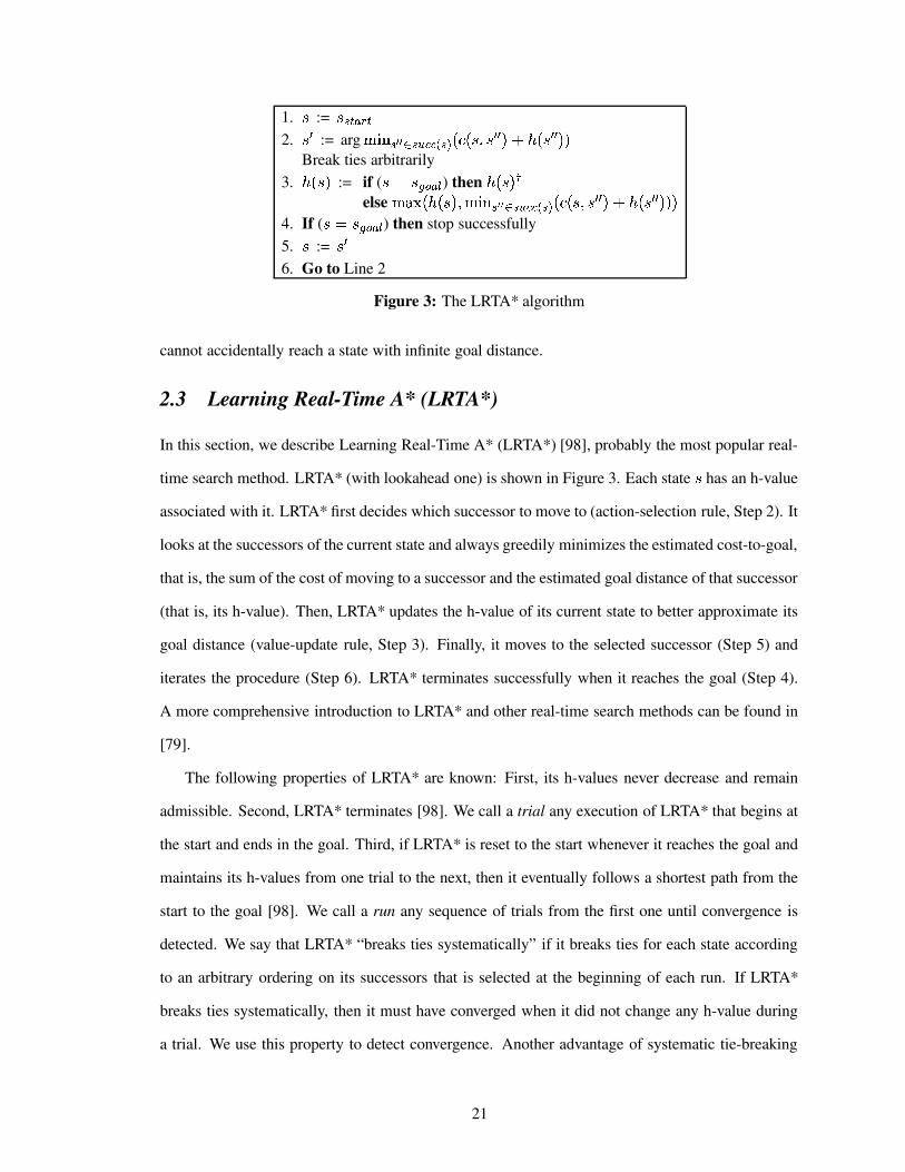
1. : := :�rtsIu+vws2. : D := arg �� I¡ r'¢ ¢�£@r'¤�¥'¥w¦Xr¨§ %©=@%�:{(c: D D , ��� %�: D D ,4,
Break ties arbitrarily3. � %�:Y, := if ( :ª�":<xby ubz ) then � %�:Y,4«
else ��¬� % � %�:Y,b(+�� I¡ r'¢ ¢�£@r'¤�¥'¥w¦Xr¨§ %©=@%�:{(c:<D D�, �®� %�:<D DI,4,4,4. If ( :ª�":<xcy ucz ) then stop successfully5. : := : D6. Go to Line 2
Figure 3: The LRTA* algorithm
cannot accidentally reach a state with infinite goal distance.
2.3 Learning Real-Time A* (LRTA*)
In this section, we describe Learning Real-Time A* (LRTA*) [98], probably the most popular real-
time search method. LRTA* (with lookahead one) is shown in Figure 3. Each state : has an h-value
associated with it. LRTA* first decides which successor to move to (action-selection rule, Step 2). It
looks at the successors of the current state and always greedily minimizes the estimated cost-to-goal,
that is, the sum of the cost of moving to a successor and the estimated goal distance of that successor
(that is, its h-value). Then, LRTA* updates the h-value of its current state to better approximate its
goal distance (value-update rule, Step 3). Finally, it moves to the selected successor (Step 5) and
iterates the procedure (Step 6). LRTA* terminates successfully when it reaches the goal (Step 4).
A more comprehensive introduction to LRTA* and other real-time search methods can be found in
[79].
The following properties of LRTA* are known: First, its h-values never decrease and remain
admissible. Second, LRTA* terminates [98]. We call a trial any execution of LRTA* that begins at
the start and ends in the goal. Third, if LRTA* is reset to the start whenever it reaches the goal and
maintains its h-values from one trial to the next, then it eventually follows a shortest path from the
start to the goal [98]. We call a run any sequence of trials from the first one until convergence is
detected. We say that LRTA* “breaks ties systematically” if it breaks ties for each state according
to an arbitrary ordering on its successors that is selected at the beginning of each run. If LRTA*
breaks ties systematically, then it must have converged when it did not change any h-value during
a trial. We use this property to detect convergence. Another advantage of systematic tie-breaking
21
is discussed in Section 2.7.3. Our approach differs slightly from that of Korf [98] whose version
of LRTA* breaks ties non-systematically and thus finds all shortest paths from the start to the goal.
We are satisfied with finding only one shortest path. To represent the state of the art, we use LRTA*
that “breaks ties randomly,” meaning that ties are broken systematically according to orderings on
the successors that are randomized before each run.
2.4 Motivation for our new action-selection rule
The premise of this work is that convergence to an optimal solution path can be sped up by con-
sistently maintaining the focus of the search upon its long-term objective, namely an optimal path
from the start to a goal, as opposed to the short-term objective of reaching a goal as fast as possi-
ble from the current state. We thus advocate a radically different way of focusing the search. In
this section, we make this intuitive search strategy operational and motivate 1) the need for a new
action-selection rule and 2) our choice of the action-selection rule that minimizes f-values.
Because it is agent-centered, real-time search is limited to local search around the current state
of the agent [91]. In particular, this means that the agent can only expand states in its neighborhood.
In fact, in the standard approach to real-time search with lookahead one, which we adopt in this
chapter, the agent can only expand the current state. The obvious implication is that the agent must
first move to a state in order to expand it. In other words, changing the search strategy requires
changing the action-selection strategy of the agent. This is different from standard best-first search
in which any state in the OPEN list could be expanded next, since its merit only depends on its
evaluation function, not on its proximity in the search space to the previously expanded state.2
Having motivated our need for a new action-selection rule, we now motivate our specific
proposal for an f-based rule. First note that, even though it remembers heuristic values for all
visited states (in a hash table, say), real-time search does not save the search tree in memory. Doing
so may speed up state re-expansions, but at the expense of memory usage. This would only be
beneficial if expansions are time-consuming and space is not a problem. For the same reason,
¯This test could be eliminated by moving Step 4 before Step 2 so that the h-value of °4±³²'´4µ is never modified. How-
ever, we prefer the current (equivalent) formulation since it makes the value-update rule for the h-values completelysymmetrical with the value-update rule for the g-values to be introduced in FALCONS.
2A recent version of A* called PHA* also takes into account the cost of physically moving from one state to anotherin the OPEN list [39].
22

real-time search only maintains point-to-point heuristic information, namely estimates of the
shortest distance from each visited state to the goal, but it does not explicitly maintain previously
found solution paths from the start to the goal. Therefore, we would like to focus the search, if not
on an explicit solution path, at least on an area of the search space believed to contain an optimal
solution. The research question thus becomes
How to estimate, for each state, how far it is from an optimal path?
The answer is not trivial because 1) such heuristic information needs to estimate the distance
from each state to a path (not another state), and 2) no solution path is explicitly identified. We
solve this problem in the following way. Recall that the f-value �G%�:�, of a state : in A* estimates the
cost � � %�:�, of a minimum-cost path from the start to the goal constrained to go through : . The main
insight of our approach is to use the property that the f � -values of all states on any minimum-cost
path from the start to the goal are all equal to the cost � � of any minimum-cost path, while the
f � -values of all other states are all strictly larger than � � (otherwise, these states would be on some
shortest path, by definition of � � ) [59]. Since f-values estimate f � -values, and if we assume that
each state has associated with it an f-value, we propose to select actions so as to always minimize
f-values. This way, if the f-values are perfectly informed, the agent will follow directly a minimum-
cost path from the start to the goal (provided that ties among states with equal f-values are broken
in favor of states with smaller h-values, that is, in the direction of the goal state). Otherwise, since
heuristic values are continuously updated, the agent will gather more informed heuristic information
and will thus be able to switch its focus to another area of the search space that looks more likely
to contain an optimal solution. In short, we will use lowest f-values to focus the search toward
previously identified regions likely to contain an optimal solution.
Figure 4 graphically represents our new action-selection rule in comparison to that used by
LRTA*. In this figure, we have assumed that the only optimal solution is the straight line between
the start and goal states. Note that the agent has strayed off of the optimal path, as typically happens
when heuristic information is not perfect. In this case, minimizing cost-to-goal estimates, as LRTA*
does, may waste search effort in areas that do not seem likely to contain an optimal path (because,
23

Start Goal
Current MinimizeCost−To−Goal
Estimates
Start Goal
Current
Minimizef−Values
a) Action−Selection Rule of LRTA*
Optimal Solution Path
Actual Path
Optimal Solution Path
Actual Path
b) Proposed Action−Selection Rule
Figure 4: Two action-selection rules for real-time search. Curves represent iso-contours for a)cost-to-goal estimates and b) f-values.
24

despite having low cost-to-goal estimates, they also have high f-values). This is because the optimal
path from the current state to the goal may have little overlap with an optimal path from the start
state to the goal. In such cases, greedily aiming for the goal may not serve the long-term objective
of finding an optimal path. By embedding this learning objective directly into the action-selection
strategy, we expect to focus the search onto a narrower region of the search space. This reduced
number of visited states will likely be accompanied by a reduction in the total number of actions
until convergence (including repeated visits to some states).
In the next section, we show that keeping the action-selection rule of LRTA* but breaking ties
in favor of states with smaller f-values already reduces the number of actions needed to converge. In
the following section, we demonstrate that directly selecting actions that minimize f-values reduces
this number even more.
2.5 Breaking ties in favor of smaller f-values
LRTA* terminates and eventually follows a shortest path no matter how its action-selection rule
breaks ties among successors. In this section, we demonstrate, for the first time, that the tie-breaking
criterion crucially influences the convergence speed of LRTA*. We present an experimental study
that shows that LRTA* converges significantly faster to a shortest path when it breaks ties towards
successors with smallest f-values rather than, say, randomly or towards successors with largest f-
values. Recall that, in the A* search method, �G%�:Y, is equal to the sum of ��� %�:�, and � %�:Y, , for all states
: . To implement our new tie-breaking criterion, LRTA* does not have the g � -values available but
can approximate them with g-values. It can update the g-values in a way similar to how it updates
the h-values, except that it uses the predecessors instead of the successors. Note that the g-values
in our real-time search algorithms do not have the same semantics as the g-values in offline search.
Here, a g-value is an underestimate of the cost of a minimum-cost path from the start to the state, not
the cost of the best path found so far. Figure 5 shows TB-LRTA* (Tie-Breaking LRTA*), our real-
time search method that maintains g- and h-values and breaks ties towards successors with smallest
f-values, where �G%�:�,���� � %�:Y, ��� %�:�, for all states : . Remaining ties can be broken arbitrarily
(but systematically). We compared TB-LRTA* against versions of LRTA* that break ties randomly
or towards successors with largest f-values. We performed experiments in thirteen combinations
25

1. : := :�rtsIu+vws2. : D := arg �� I¡ r'¢ ¢�£@r'¤�¥'¥w¦Xr¨§ %©=@%�:{(c: D D , ��� %�: D D ,4,
Break ties in favor of a successor :�D D with a smallest f-value, where �G%�:�D DZ,¶��� � %�:3D D�, ��� %�:3D D�,Break remaining ties arbitrarily (but systematically)
3. � %�:�, := if ( :ª�":�rtsIu+vws ) then � %�:Y,else ��¬�·% � %�:�,b(+�¸ I¡ rt¢ ¢I£fR3vw¹¨º?¦Zr³§ % � %�: D D , � =@%�: D D (c:Y,4,4,
� %�:Y, := if ( :ª�":<xby ubz ) then � %�:Y,else ��¬� % � %�:Y,b(+�� I¡ r ¢ ¢ £@r'¤�¥'¥w¦Xr¨§ %©=@%�:{(c:<D D�, �®� %�:<D DI,4,4,
4. If ( :ª�":<xcy ucz ) then stop successfully5. : := : D6. Go to Line 2
Figure 5: The TB-LRTA* algorithm
of standard search domains from the artificial intelligence literature and heuristic values, averaged
over at least one thousand runs each. Section 2.7 contains information on the domains, heuristic
values, and experimental setup, including how we tested for statistical significance. Table 3 shows
that in all cases but one (Permute-7 with the zero (Z) heuristic)3 breaking ties towards successors
with smallest f-values (statistically) significantly sped up the convergence of LRTA* in terms of
travel cost (action executions).
2.6 FALCONS: Selecting actions that minimize f-values
In this section, we show that turning f-value minimization into the primary action-selection criterion
is not trivial. The obvious, naive approach leads to non-termination or convergence to a non-optimal
path. We then show how to solve these problems in our final version of FALCONS.
2.6.1 FALCONS: A naive approach
We just showed that TB-LRTA* converges significantly faster than LRTA* because it breaks ties
towards successors with smallest f-values. We thus expect real-time search methods that imple-
ment this principle more consequently and always move to successors with smallest f-values to
converge even faster. Figure 6 shows Naive FALCONS (FAst Learning and CONverging Search),
our real-time search method that maintains g- and h-values, always moves to successors with small-
est f-values, and breaks ties to minimize the estimated cost-to-goal. Remaining ties can be broken
3This exception will disappear in our results with FALCONS.
26

Table 3: Travel cost to convergence with different tie-breaking rules
domain and LRTA* that breaks ties . . .heuristic towards randomly towards a smallestvalues a largest f-value f-value (TB-LRTA*)
8-Puzzle M 64,746.47 45,979.19 18,332.39T 911,934.40 881,315.71 848,814.91Z 2,200,071.25 2,167,621.63 2,141,219.97
Gridworld N 116.50 97.32 82.08Z 1,817.57 1,675.87 1,562.46
Permute-7 A 302.58 298.42 288.62Z 16,346.56 16,853.69 16,996.51
Arrow F 1,755.42 1,621.26 1,518.27Z 7,136.93 7,161.71 7,024.11
Tower of D 145,246.55 130,113.43 116,257.30Hanoi Z 156,349.86 140,361.39 125,332.52Words L 988.15 813.66 652.95
Z 16,207.19 16,137.67 15,929.81
arbitrarily (but systematically). To understand why ties are broken to minimize the estimated cost-
to-goal, consider g- and h-values that are perfectly informed. In this case, all states on a shortest
path have the same (smallest) f-values and breaking ties to minimize the estimated cost-to-goal en-
sures that Naive FALCONS moves towards the goal. (All real-time search methods discussed in
this chapter have the property that they follow a shortest path right away if the g- and h-values are
perfectly informed.) To summarize, Naive FALCONS is identical to TB-LRTA* but switches the
primary and secondary action-selection criteria. Unfortunately, we show in the remainder of this
section that Naive FALCONS does not necessarily terminate nor converge to a shortest path. In
both cases, this is due to Naive FALCONS being unable to increase misleading f-values of states
that it visits, because they depend on misleading g- or h-values of states that it does not visit and
thus cannot increase.
Naive FALCONS can cycle forever. Figure 7 shows an example of a domain where Naive
FALCONS does not terminate for g- and h-values that are admissible but inconsistent. Naive FAL-
CONS follows the cyclic path :YN�(c:{13(c:<5�(c:�»Y(c:<5�(c:�»�(QPQPQP without modifying the g- or h-values of any
state. For example during the first trial, Naive FALCONS updates � %�:�5<, to one (based on � %�:Y¼3, ) and
� %�:�5<, to one (based on � %�:�½3, ), and thus does not modify them. � %�:{¼3, and � %�:�½<, are both zero and
27
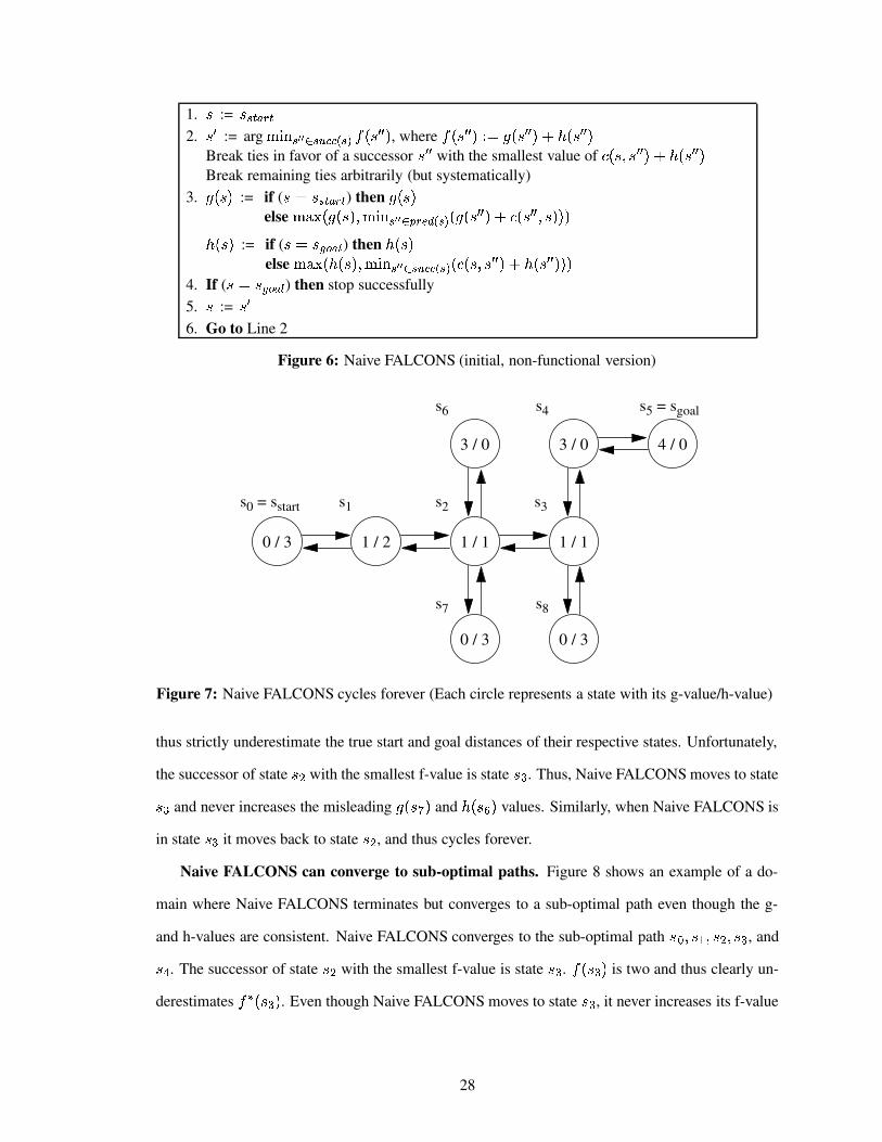
1. : := :�rtsIu+vws2. : D := arg �� I¡ r'¢ ¢I£@r'¤�¥'¥w¦Xr¨§ �G%�: D D , , where �G%�: D D ,¾��� � %�: D D , ��� %�: D D ,
Break ties in favor of a successor :�D D with the smallest value of =@%�:{(c:�D DI, ��� %�:3D D�,Break remaining ties arbitrarily (but systematically)
3. � %�:�, := if ( :ª�":�rtsIu+vws ) then � %�:Y,else ��¬�·% � %�:�,b(+�¸ I¡ rt¢ ¢I£fR3vw¹¨º?¦Zr³§ % � %�: D D , � =@%�: D D (c:Y,4,4,
� %�:Y, := if ( :ª�":<xby ubz ) then � %�:Y,else ��¬� % � %�:Y,b(+�� I¡ r ¢ ¢ £@r'¤�¥'¥w¦Xr¨§ %©=@%�:{(c:<D D�, �®� %�:<D DI,4,4,
4. If ( :ª�":<xcy ucz ) then stop successfully5. : := : D6. Go to Line 2
Figure 6: Naive FALCONS (initial, non-functional version)
3 / 0 3 / 0
0 / 3 0 / 3
1 / 1 1 / 1
s5 = sgoal
0 / 3 1 / 2
4 / 0
s0 = sstart s1 s2 s3
s4s6
s8s7
Figure 7: Naive FALCONS cycles forever (Each circle represents a state with its g-value/h-value)
thus strictly underestimate the true start and goal distances of their respective states. Unfortunately,
the successor of state : 5 with the smallest f-value is state : » . Thus, Naive FALCONS moves to state
:�» and never increases the misleading � %�:{¼3, and � %�:�½<, values. Similarly, when Naive FALCONS is
in state : » it moves back to state : 5 , and thus cycles forever.
Naive FALCONS can converge to sub-optimal paths. Figure 8 shows an example of a do-
main where Naive FALCONS terminates but converges to a sub-optimal path even though the g-
and h-values are consistent. Naive FALCONS converges to the sub-optimal path :�N�(c:@13(c:�5�(c:<» , and
:<¿ . The successor of state : 5 with the smallest f-value is state : » . �G%�: » , is two and thus clearly un-
derestimates � � %�:�»<, . Even though Naive FALCONS moves to state :{» , it never increases its f-value
28
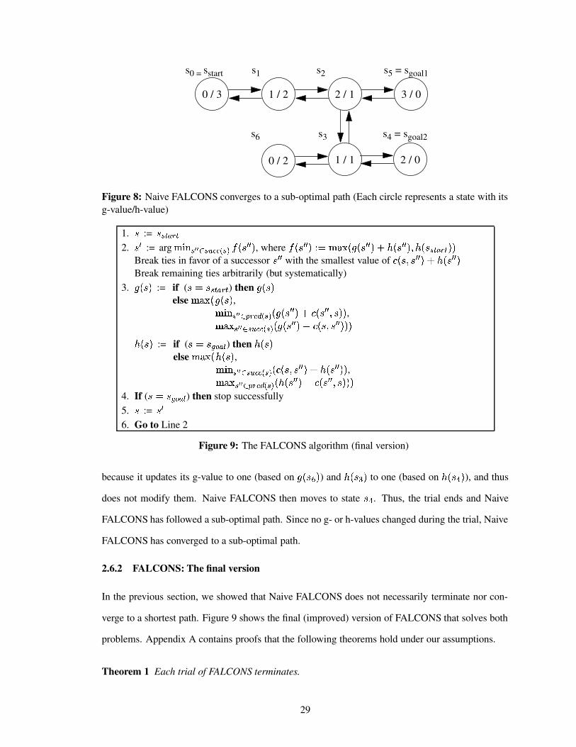
1 / 1
2 / 10 / 3 1 / 2
2 / 0
s0 = sstart s1 s2
s3
3 / 0
0 / 2
s4 = sgoal2
s5 = sgoal1
s6
Figure 8: Naive FALCONS converges to a sub-optimal path (Each circle represents a state with itsg-value/h-value)
1. : := :�rtsIu+vws2. : D := arg �� I¡ r'¢ ¢I£@r'¤�¥'¥w¦Xr¨§ �G%�: D D , , where �G%�: D D ,¾�����¸¬�H% � %�: D D , ��� %�: D D ,b( � %�:�r'sIucv¨sw,4,
Break ties in favor of a successor :�D D with the smallest value of =@%�:{(c:�D DI, ��� %�:3D D�,Break remaining ties arbitrarily (but systematically)
3. � %�:�, := if ( :À�":Yr'sIucvws ) then � %�:�,else ��¬�·% � %�:Y, ,
�� I¡ rt¢ ¢�£fRQv4¹¨º?¦Xr¨§ % � %�:<D DI, � =@%�:3D D©(c:�,4, ,��¬� rt¢ ¢�£@r'¤<¥t¥w¦Xr¨§ % � %�:<D D�,)Á�=Y%�:�(c:<D D�,4,4,
� %�:Y, := if ( :ª�":<xcy ucz ) then � %�:Y,else ��¬� % � %�:�, ,
�� I¡ rt¢ ¢�£Yrt¤<¥'¥w¦Zr³§ %©=@%�:�(c:3D D�, ��� %�:3D DI,4, ,��¬� r'¢ ¢I£?RQv4¹³º?¦Zr³§ % � %�:<D DI,AÁ�=Y%�:<D D©(c:�,4,4,
4. If ( :ª�":<xcy ucz ) then stop successfully5. : := : D6. Go to Line 2
Figure 9: The FALCONS algorithm (final version)
because it updates its g-value to one (based on � %�: ½ , ) and � %�: » , to one (based on � %�:�¿�, ), and thus
does not modify them. Naive FALCONS then moves to state : ¿ . Thus, the trial ends and Naive
FALCONS has followed a sub-optimal path. Since no g- or h-values changed during the trial, Naive
FALCONS has converged to a sub-optimal path.
2.6.2 FALCONS: The final version
In the previous section, we showed that Naive FALCONS does not necessarily terminate nor con-
verge to a shortest path. Figure 9 shows the final (improved) version of FALCONS that solves both
problems. Appendix A contains proofs that the following theorems hold under our assumptions.
Theorem 1 Each trial of FALCONS terminates.
29

Theorem 2 FALCONS eventually converges to a path from the start to the goal if it is reset to the
start whenever it reaches the goal and maintains its g- and h-values from one trial to the next one.
Theorem 3 The path from the start to the goal that FALCONS eventually converges to is a shortest
path.
We now give some intuitions behind the new value-update and action-selection rules and show
that they solve the problems of Naive FALCONS for the examples introduced in the previous sec-
tion.
FALCONS terminates. The new value-update rules of FALCONS cause it to terminate. We
first derive the new value-update rule for the h-values. It provides more informed but still admissible
estimates of the h-values than the old value-update rule, by making better use of information in the
neighborhood of the current state. The new value-update rule makes the h-values locally consistent
and is similar to the pathmax equation used in conjunction with A* [121]. If the h-values are
consistent, then there is no difference between the old and new value-update rules. To motivate the
new value-update rule, assume that the h-values are admissible and FALCONS is currently in some
state : with :���":�xcy ucz . The old value-update rule used two lower bounds on the goal distance of state
: , namely � %�:�, and �� �¡ r'¢ ¢I£@r'¤<¥t¥w¦Xr¨§ %©=@%�:{(c: D D , �Â� %�: D D ,4, . The new value-update rule adds a third lower
bound, namely ��¬� rt¢ ¢j£fRQv4¹¨º?¦Xr¨§ % � %�:3D D�,ÃÁ�=Y%�:<D D©(c:�,4, . To understand the third lower bound, note that the
goal distance of any predecessor : D D of state : is at least � %�: D D , since the h-values are admissible.
This implies that the goal distance of state : is at least � %�:@D D�,¶ÁÂ=@%�:3D D©(c:�, . Since this is true for all
predecessors of state : , the goal distance of state : is at least ��¬� rt¢ ¢I£fR3vw¹¨º?¦Zr³§ % � %�: D D ,)Á_=Y%�: D D (c:Y,4, . The
maximum of the three lower bounds then is an admissible estimate of the goal distance of state :and thus becomes its new h-value. This explains the new value-update rule for the h-values. The
new value-update rule for the g-values can be derived in a similar way.
As an example, we show that Naive FALCONS with the new value-update rules now terminates
in the domain from Figure 7. When Naive FALCONS is in state :�5 during the first trial, it increases
both � %�:�5<, and � %�:�5<, to two and then moves to state :Y» . The successor of state :Y» with the smallest
f-value is state : ¿ , and no longer state :�5 , because �G%�:�5Q, was increased to four. Thus, Naive FAL-
CONS now moves to state : ¿ and breaks the cycle. Unfortunately, the new value-update rules are
30

not sufficient to guarantee that Naive FALCONS converges to a shortest path. The domain from
Figure 8 still provides a counterexample.
FALCONS converges to a shortest path. The new action-selection rule of FALCONS causes
it to converge to a shortest path by using more informed but still admissible estimates of the f � -values. In the following, we assume that the g- and h-values are admissible and we present two
lower bounds on � � %�:Y, . First, � � %�:�, is at least � %�:�, �� %�:�, , since the g- and h-values are admissible.
Second, � � %�:Y, is at least as large as the cost of a shortest path from the start to the goal, a lower
bound of which is � %�: r'sIucv¨s , , since the h-values are admissible. The maximum of the two lower
bounds is an admissible estimate of � � %�:�, and thus becomes the new f-value of : . This explains
the new calculation of the f-values performed by the action-selection rule. The other parts of the
action-selection rule remain unchanged. The new f-value of state : , unfortunately, cannot be used
to update its g- or h-values, because it is unknown by how much to update the g-value and by how
much to update the h-value.
As an example, we show that FALCONS now converges to a shortest path in the domain from
Figure 8. When FALCONS reaches state :@5 in the first trial, �G%�:�»3, is now three. All three successors
of state : 5 have the same f-value and FALCONS breaks ties in favor of the one with the smallest
h-value, namely state :�Š. Thus, the trial ends and FALCONS has followed a shortest path. Since no
g- or h-values changed, FALCONS has converged to a shortest path.
2.7 Experimental results
In this section, we present our empirical evaluation of FALCONS, which we compared to LRTA*
that breaks ties randomly and TB-LRTA*. We describe, in turn, our domains and heuristic functions,
our performance measures, our empirical setup, and finally our results.
2.7.1 Domains and heuristics
For our empirical study, we used the following domains from the artificial intelligence literature.
The 8-Puzzle domain [98] consists of eight tiles (numbered one through eight) in a 3x3 grid,
leaving one position blank. A move is performed by sliding one of the tiles adjacent to the blank into
the blank position. Since tiles are not allowed to move diagonally, the number of possible moves in
31
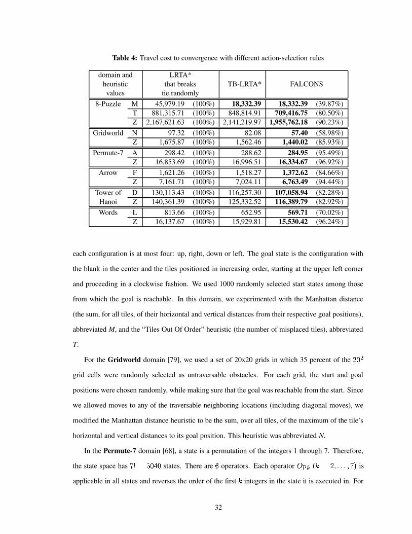
Table 4: Travel cost to convergence with different action-selection rules
domain and LRTA*heuristic that breaks TB-LRTA* FALCONSvalues tie randomly
8-Puzzle M 45,979.19 (100%) 18,332.39 18,332.39 (39.87%)T 881,315.71 (100%) 848,814.91 709,416.75 (80.50%)Z 2,167,621.63 (100%) 2,141,219.97 1,955,762.18 (90.23%)
Gridworld N 97.32 (100%) 82.08 57.40 (58.98%)Z 1,675.87 (100%) 1,562.46 1,440.02 (85.93%)
Permute-7 A 298.42 (100%) 288.62 284.95 (95.49%)Z 16,853.69 (100%) 16,996.51 16,334.67 (96.92%)
Arrow F 1,621.26 (100%) 1,518.27 1,372.62 (84.66%)Z 7,161.71 (100%) 7,024.11 6,763.49 (94.44%)
Tower of D 130,113.43 (100%) 116,257.30 107,058.94 (82.28%)Hanoi Z 140,361.39 (100%) 125,332.52 116,389.79 (82.92%)Words L 813.66 (100%) 652.95 569.71 (70.02%)
Z 16,137.67 (100%) 15,929.81 15,530.42 (96.24%)
each configuration is at most four: up, right, down or left. The goal state is the configuration with
the blank in the center and the tiles positioned in increasing order, starting at the upper left corner
and proceeding in a clockwise fashion. We used 1000 randomly selected start states among those
from which the goal is reachable. In this domain, we experimented with the Manhattan distance
(the sum, for all tiles, of their horizontal and vertical distances from their respective goal positions),
abbreviated M, and the “Tiles Out Of Order” heuristic (the number of misplaced tiles), abbreviated
T.
For the Gridworld domain [79], we used a set of 20x20 grids in which 35 percent of the !Ym 5
grid cells were randomly selected as untraversable obstacles. For each grid, the start and goal
positions were chosen randomly, while making sure that the goal was reachable from the start. Since
we allowed moves to any of the traversable neighboring locations (including diagonal moves), we
modified the Manhattan distance heuristic to be the sum, over all tiles, of the maximum of the tile’s
horizontal and vertical distances to its goal position. This heuristic was abbreviated N.
In the Permute-7 domain [68], a state is a permutation of the integers 1 through 7. Therefore,
the state space has �aÆH� � mYÇ{m states. There are È operators. Each operator É^[AÊ�%�Ë��O!�(QPQPQP<(b�@, is
applicable in all states and reverses the order of the first Ë integers in the state it is executed in. For
32

example, the execution of É^[ ¿ in state �YÈ � Ç�Ì@!�� leads to state Ç � È{�YÌ@!�� . The goal state is �3!@Ì�Ç � È{� .The adjacency heuristic (abbreviated A) computes for each state : the number of pairs of adjacent
digits in the goal state that are not adjacent in : . For instance, Í-%'�YÌ@!��3È�Ç � ,Î�KÌ since exactly three
pairs are adjacent in the goal but not in : , namely %�Ì�(4Ça, , % � (cÈ{, and %�È�(b�@, . We experimented with all
5040 states as start state.
We also used a version of the Tower of Hanoi domain [68] with 7 disks and 3 pegs. In the goal
state, all disks are on the same peg, say peg number three. We experimented with 1000 randomly
chosen start states. The D heuristic simply counts the number of disks that are not on the goal peg.
The Words domain [70] is a connected graph whose 4493 nodes are 5-letter English words
that are pairwise connected if they differ in exactly one letter. The goal state is the word “goals”.
We experimented with 1000 randomly chosen start states. The L heuristic computes the number of
positions (between 1 and 5) for which the letter is different from the letter at the same position in
the goal state.
In the Arrow domain [95], a state is an ordered list of 12 arrows. Each arrow can either point
up or down. There are 11 operators that can each invert a pair of adjacent arrows. The goal state
has all arrows pointing up. We experimented with 1000 randomly chosen start states among those
from which the goal is reachable. The F heuristic returns the largest integer that is not larger than
the number of arrows that need to be flipped divided by two.
In addition to the above domain-dependent heuristic values, we also experimented in all domains
with the constant function Zero (Z). Note that all of our domains share the following two properties:
(1) they are undirected, which means that for every action leading from state : to state :aD with cost = ,there is a reverse action from : D to : with cost = , and (2) they have uniform costs, which means that
all action costs are one. Finally, all of these domains and heuristic functions satisfy our assumptions.
2.7.2 Performance measures
So far, we have motivated our new action-selection rule in terms of an expected reduction in the
runtime to convergence. In this section, we discuss this and other relevant performance measures.
Number of actions until convergence. The number of expansions is a common way of mea-
suring the performance of heuristic search algorithms in general [131, 96, 105]. Since real-time
33

heuristic search with lookahead one only expands the states it visits, the number of expansions is
equal to the number of actions it executes. The number of actions until convergence (also referred
to as “travel cost to convergence”) is therefore our primary performance measure in this chapter.
The reason this performance measure is used in lieu of the runtime itself is because the latter is
typically sensitive to both the implementation and the architecture of the machine on which it is
run. In contrast, the number of actions depends only on the algorithm itself and thus makes it easier
for different research teams to compare and reproduce empirical results. Nevertheless, since the
time needed for each action selection is bounded by a constant (in domains with a finite maximum
branching factor), the total runtime of real-time search algorithms is equal to the product of this
constant and of our primary performance measure. A decrease in the latter must be weighed against
any increase of the constant itself.
Number of trials until convergence. Since a real-time search agent is reset into the start state
whenever it reaches the goal, its behavior is episodic. We have called each episode a trial. So far,
we have implicitly assumed that the total time until convergence is equal to the sum of the times
spent in all trials. This assumes that the inter-trial time is negligible. However, there are domains
(for example, when a robot is learning to juggle) in which resetting the agent into its initial state is
time-consuming. In such domains, reducing the number of trials may significantly reduce the total
learning time in practice. In other cases, such as robot simulations, inter-trial time is negligible. To
take this factor into account in a domain-independent way, we propose to use the number of trials
until convergence as another performance measure.
Number of actions in the first trial. In the learning behavior of real-time search agents, there
is a possible trade-off between how many times they reach the goal (that is, the number of trials)
and how much effort they spend reaching the goal (that is, the effort per trial). It is possible that
additional exploration of the state space within a trial will reduce the total number of trials needed
to converge. This is a trade-off between short-term (getting to the goal as fast as possible) and long-
term (converging to an optimal solution) objectives. We therefore propose to measure the effort
spent in the first trial as an indication of how much exploration is performed at the beginning of
learning. Our last performance measure will thus be the number of actions in the first trial.
34

2.7.3 Empirical setup
In order for FALCONS to converge to a unique path, the secondary tie-breaking criterion must
be systematic (systematic tie-breaking was defined in Section 2.3). We enforced systematicity by
(1) choosing an arbitrary ordering for the successors of each state and (2) breaking remaining ties
according to that ordering. The ordering was selected randomly at the beginning of a run and did
not change during the run.
An experiment refers to a sequence of � runs of an algorithm in one domain with a given set
of heuristic values. To attain statistical significance, we averaged our results over ���Qm@m@m runs,
except in the Permute-7 domain for which each experiment consisted of �aÆ)� � mYÇ{m runs, one for
each possible start state. In general, the � runs of an experiment only differed from the other runs in
the same experiment in two respects: (1) the start state, and (2) the random ordering selected at the
beginning of each run to be used for systematic tie-breaking. In addition, in the Gridworld domain,
each run used a different grid and goal state.
There are two advantages to using systematic tie-breaking. First, it ensures that FALCONS will
converge to a unique path. If tie-breaking is not systematic, then FALCONS may not converge to
a unique path. Instead, it may converge to a set of shortest paths and randomly switch between
them after the heuristic values have converged, just like LRTA* [98]. Systematic tie-breaking thus
facilitated the detection of convergence, which happens when no heuristic value changes in the
course of a run.
Second, systematic tie-breaking allowed us to carefully control our experimental conditions. In
particular, we compared pairs of experiments that only differed in the algorithm tested (for exam-
ple, FALCONS versus LRTA*). We only compared pairs of experiments in the same domain and
with the same heuristic values. In addition, we used the same (random) ordering of successor states
for systematic tie-breaking in all pairs of runs to be compared. In other words, when comparing
algorithm 1 with algorithm 2, run 1 of both experiments used the same ordering, run 2 of both
experiments used the same ordering (but different from that of run 1), etc. Furthermore, each pair
of corresponding runs used the same start state (and the same grid and goal state in the Gridworld
domain). Now, assume that we wanted to compare the travel cost to convergence of FALCONS in a
35

Table 5: Trials to convergence with different action-selection rules
domain and LRTA*heuristic that breaks TB-LRTA* FALCONSvalues tie randomly
8-Puzzle M 214.37 (100%) 58.30 58.30 (27.20%)T 1,428.57 (100%) 1,214.63 797.26 (55.81%)Z 1,428.59 (100%) 1,227.74 756.47 (52.95%)
Gridworld N 6.06 (100%) 5.01 2.90 (47.85%)Z 32.02 (100%) 26.30 19.77 (61.74%)
Permute-7 A 26.91 (100%) 25.55 22.10 (82.13%)Z 117.82 (100%) 92.63 75.22 (63.84%)
Arrow F 114.94 (100%) 110.60 89.01 (77.44%)Z 171.50 (100%) 135.13 105.92 (61.76%)
Tower of D 214.47 (100%) 177.96 109.13 (50.88%)Hanoi Z 216.77 (100%) 166.55 101.44 (46.80%)Words L 32.82 (100%) 22.72 18.40 (56.06%)
Z 71.86 (100%) 55.77 50.10 (69.72%)
particular domain and with a particular set of heuristic values (experiment 1) with that of LRTA* in
the same domain and with the same set of heuristic values (experiment 2). Our experimental setup
guaranteed that the only difference between run V ( V)�F�Y(QPQPQP<(4� ) of experiment 1 and run V of exper-
iment 2 was the algorithm tested, whereas each run was made under different conditions (namely,
start state and ordering of successor states) from all of the other runs in the same experiment. This
setup enabled us to test our results for statistical significance using the paired-samples Z test.
2.7.4 Results
Tables 4, 5, and 6 report the travel cost (action executions) until convergence, the number of trials
until convergence, and the travel cost of the first trial, respectively.
Table 4 shows that, in all cases, FALCONS converged to a shortest path with a smaller travel
cost (action executions) than LRTA* that breaks ties randomly and, in all cases but one, faster than
TB-LRTA*. The percentages in the last column compare the travel cost of FALCONS with that of
LRTA*. FALCONS converged 18.57 percent faster over all thirteen cases and in one case even 60.13
percent faster. All the comparisons stated above are significant at the five-percent confidence level.
The heuristic values for each domain are listed in order of their decreasing informedness (sum of
36

Table 6: Travel cost of the first trial with different action-selection rules
domain and LRTA*heuristic that breaks TB-LRTA* FALCONSvalues tie randomly
8-Puzzle M 311.18 (100%) 452.84 452.84 (145.52%)T 1,342.75 (100%) 970.87 1,057.86 (78.78%)Z 81,570.22 (100%) 81,585.44 81,526.34 (99.95%)
Gridworld N 12.15 (100%) 12.70 20.92 (172.18%)Z 182.37 (100%) 182.55 183.13 (100.42%)
Permute-7 A 8.14 (100%) 7.75 8.13 (99.88%)Z 2,637.86 (100%) 2,639.13 2,639.13 (100.05%)
Arrow F 15.85 (100%) 16.62 33.61 (212.05%)Z 1,016.33 (100%) 1,016.83 1,016.83 (100.05%)
Tower of D 4,457.86 (100%) 3,654.80 3,910.46 (87.72%)Hanoi Z 4,839.49 (100%) 4,803.81 4,801.84 (99.22%)Words L 24.27 (100%) 27.79 37.80 (155.75%)
Z 2,899.73 (100%) 2,900.36 2,900.68 (100.03%)
the heuristic values over all states). For example, the (completely uninformed) zero (Z) heuristic is
listed last. Table 4 then, shows that the speedup of FALCONS over LRTA* was positively correlated
with the informedness of the heuristic values. This suggests that FALCONS makes better use of the
given heuristic values. Notice that it cannot be the case that FALCONS converges more quickly
than LRTA* because it looks at different (or more) states than LRTA* when selecting successor
states. FALCONS looks at both the predecessors and successors of the current state while LRTA*
looks only at the successors, but all of our domains are undirected and thus every predecessor is
also a successor. This implies that FALCONS and LRTA* look at exactly the same states.
Table 5 shows that, in all cases, FALCONS converged to a shortest path with a smaller number
of trials than LRTA* that breaks ties randomly and, in all cases but one, faster than TB-LRTA*.
FALCONS converged 41.94 percent faster over all thirteen cases and in some cases even 72.80
percent faster.
To summarize, Table 4 and Table 5 show that FALCONS converges faster than LRTA* and even
TB-LRTA*, both in terms of travel cost and trials.
We originally expected that FALCONS would increase the travel cost during the first trial, since
the action-selection rule of LRTA* (minimize the cost-to-goal) has experimentally been shown to
37

Table 7: Travel cost to convergence with different action-selection rules, and with or without gupdates for FALCONS
domain and FALCONSheuristic LRTA* FALCONS withoutvalues � updates
8-Puzzle M 45,979.19 (100%) 18,332.39 (39.87%) 19,222.08 (41.81%)T 881,315.71 (100%) 709,416.75 (80.50%) 817,078.12 (92.71%)
Gridworld N 97.32 (100%) 57.40 (58.98%) 58.82 (60.44%)Permute-7 A 298.42 (100%) 284.95 (95.49%) 263.00 (88.13%)Arrow F 1,621.26 (100%) 1,372.62 (84.66%) 1,533.11 (94.56%)T. of Hanoi D 130,113.43 (100%) 107,058.94 (82.28%) 128,987.97 (99.14%)Words L 813.66 (100%) 569.71 (70.02%) 547.35 (67.27%)
result in a small travel cost during the first trial under various conditions. Table 6 shows that, in
four of the thirteen cases, the travel cost of FALCONS during the first trial was larger than that of
LRTA*; in seven cases it was approximately the same (99 percent to 101 percent); and in two cases
it was lower. The travel cost of FALCONS during the first trial was 19.35 percent larger than that of
LRTA* over the thirteen cases. Overall, there is no systematic relationship between the travel cost
of FALCONS and LRTA* during the first trial, and the sum of planning and plan-execution times is
always small for FALCONS, just like for LRTA*.
So far, our main performance measure has been the travel cost to convergence. One may com-
plain that the speedup exhibited by FALCONS over LRTA* comes at an extra computational cost,
namely an extra value update per action execution. To decrease the total computational cost (value
updates), FALCONS would have to cut the travel cost to convergence at least in half. However, it re-
duces the travel cost by only 18.57 percent. We also compared FALCONS with a variant of LRTA*
that performs two value updates per action execution. This can be done in various ways. Among the
ones we tried, our best results were obtained with a variant of LRTA* that first updates � %�:�DI, (where
: D is the successor of the current state : with the smallest =Y%�:�(c: D , �� %�: D , ), then updates � %�:�, , and
finally selects the successor :YD D of : with the smallest =@%�:�(c:�D D�, �� %�:<D D�, , which may be different from
: D . Empirically, this algorithm had a smaller travel cost to convergence than FALCONS.
However, we can modify FALCONS so that it never updates the g-values, resulting in one
value-update per action execution, just like LRTA*. Table 7 reports experimental results that clearly
38
show that FALCONS without g updates had a smaller travel cost to convergence than LRTA* (with
lookahead one). The speedup was 22.28 percent on average, and up to 58.19 percent. Additional
results show that the number of trials to convergence for FALCONS without g updates was 25.97
percent less than for LRTA* on average (and up to 68.71 percent less), and that FALCONS executed
an average of 57.51 percent more actions than LRTA* in the first trial.3 These results are important
for two reasons. First, they support the claim that the action-selection rule of FALCONS speeds up
convergence by making better use of the available heuristic knowledge and is able to decrease both
the travel cost and computational cost to convergence. Second, they suggest that FALCONS may
benefit from an enhanced action-selection rule that focuses the search even more sharply around an
optimal path by speeding up the learning of more accurate g-values, while still making efficient use
of the initial heuristic knowledge.
2.8 Related work
[79] presents an overview of real-time heuristic search algorithms and their application to moving-
target search [81, 76, 82, 152] and bidirectional search [77, 78]. Multi-agent extensions of real-time
search have also been discussed [89, 87, 171, 80]. We now focus on single-agent real-time search
approaches that are more closely related to LRTA* and FALCONS.
HLRTA* [164] is representative of a class of methods (such as ELRTA* [164] and SLRTA*
[34]) that speed up the convergence of LRTA* by using a different value-update rule.4 This is in
contrast to FALCONS that uses a different action-selection rule. Both improvements to LRTA*
are orthogonal and guarantee the optimality of the final (that is, converged) solution. In [51, 46],
we present the first thorough empirical evaluation of HLRTA* and show that it and FALCONS
have complementary strengths that can be combined. We call the resulting real-time search method
eFALCONS (for Even FAster Learning and CONverging Search) and show that it converges with
fewer actions to a minimum-cost plan than LRTA*, HLRTA*, and FALCONS, even though it looks
3In domains with uniform costs, with consistent h-values, and with zero-initialized g-values, FALCONS without gupdates reduces to LRTA*. Thus, Table 7 does not show results for completely uninformed heuristic values and ouraverages do not include them.
4We thank Stefan Edelkamp for introducing us to HLRTA* and Richard Korf for making Thorpe’s thesis aboutHLRTA* available to us.
39

at the same states when it selects successors on undirected graphs and is not more knowledge-
intensive to implement. However, the main drawback of eFALCONS is that its runtime overhead
per state expansion is larger than that of its component algorithms since it maintains more heuristic
values per state. This overhead is typically larger than the runtime savings due to the reduction in
the number of actions to convergence.Ò-search is another variant of LRTA* that uses a pruning mechanism to control its exploration
[153]. This mechanism is orthogonal to the aforementioned improvements on LRTA*. Shimbo et al.
show that FALCONS converges faster thanÒ-search in the 8-Puzzle and gridworld domains.5 Fur-
thermore, their experiments demonstrate that FALCONS significantly reduces space requirements
over LRTA*. This is important since it provides empirical evidence that the speedup exhibited by
FALCONS is accompanied by a sharper focus of the search around the optimal solution it converges
to. [153] also introduces another variant of LRTA* called Ó -search that speeds up its convergence
while sacrificing the optimality of the converged solution by putting more weight on the h-values
when computing the estimated cost to the goal. Again, this variation is orthogonal to the aforemen-
tioned ones.
Finally, there exists a class of real-time search algorithms that add a backtracking mechanism
to LRTA* in order to speed up convergence by propagating value updates backward. This class
includes SLA* [155], SLA*T [156], and Ô -Trap [17]. SLA* and Ô -Trap use essentially the same
backtracking strategy but were developed independently. SLA*T, which extends SLA* with an ad-
ditional parameter to control the amount of backtracking and thus the amount of exploration (and
the rate of learning), was applied to project scheduling problems with resource constraints (PSRC).
The idea of backtracking is orthogonal to the action-selection rule used by FALCONS. However,
all the backtracking algorithms make the extra assumption that all actions in the domain are re-
versible (that is, the graph is undirected). In contrast, FALCONS is applicable to both undirected
and directed graphs.
5Nevertheless, Õ -search does converge faster than LRTA*, even though the motivation for it was different ( Õ -searchwas designed to distribute and control the learning across trials).
40
2.9 Future work
We envision at least two directions for future work in real-time search.
First, the family of real-time search algorithms has grown quite large. There is a need for an
exhaustive empirical comparison of these algorithms. Due to the different assumptions they make,
this empirical study will require a wide variety of benchmark domains6 in order to discover a map-
ping between classes of domains (based, for example, on structural features of their associated state
spaces) and the classes of algorithms that are most efficient on them. Not only is the efficiency of
real-time search algorithms expected to be domain-dependent, there are numerous ways to measure
performance (such as the number of actions to convergence or per trial, the number of trials to con-
vergence, the solution quality as a function of learning or after convergence, the rate of learning,
the trade-off between exploration and exploitation, etc.). Furthermore, most of the foregoing en-
hancements to LRTA* are orthogonal, including changes to the value-update rule, changes to the
action-selection rule, the increased weight on the h-values, the addition of pruning rules, the use of
a larger and even variable lookahead [17], etc.). The number of algorithms resulting from possible
combinations is extremely large. Yet, it would be useful to know which combinations work best
together and for what tasks. [16] has started such an investigation.
Second, a particularly interesting extension of FALCONS is its application to domains from
real-time control. These domains require real-time action selection and convergence to optimal
behaviors but, at the same time, the setup for each trial is expensive and thus it is important to
keep the number of trials small. For learning how to balance poles or juggle devil-sticks [146],
for example, the pole needs to be picked up and brought into the initial position before every trial.
Domains from real-time control are typically directed and sometimes probabilistic, and we have
not yet applied FALCONS to domains with these properties. Of course, FALCONS can be applied
without modification to directed domains since all of our theoretical results continue to hold. The
main difficulty of applying FALCONS to probabilistic domains is to adapt the notion of f-values to
such domains. When the effects of actions are probabilistic, the agent learns a policy that only has
a probability (typically smaller than one) of visiting some states. In this context, it is not obvious
6Note that all the domains used in our evaluation of FALCONS happen to be undirected.
41
how to even define the concept of a minimum path cost through a state (such as an f-value) when
the policy is not guaranteed to visit the state.
2.10 Contributions
Our research on real-time heuristic search has yielded the following contributions:
k We have extended the scope of applicability of A*’s principle for ordering state expansions
to the real-time search setting. We have shown that, by making real-time search less greedy
(namely, by moving towards states with minimum f-values instead of h-values), we can sig-
nificantly reduce its number of actions to convergence in several domains. Furthermore, this
reduction in runtime can be accompanied by a reduction in the number of visited states, and
therefore in the space requirements of real-time search, as results in [153] indicate.
k We designed a new action-selection rule for online, dynamic programming methods. We
have shown how to implement it in the case of deterministic task domains. This rule has
great potential relevance to the reinforcement-learning community, since the vast majority of
existing methods in this area use the greedy action-selection rule when exploiting heuristic
information. Our results suggest that significantly faster learning could result from a less
greedy exploitation rule.
k We successfully implemented FALCONS, a new algorithm for real-time heuristic search.
FALCONS exhibits significantly higher performance than state-of-the-art real-time heuristic
search methods. More precisely, FALCONS reduces both the number of actions and the
number of trials it takes to converge. We resolved non-trivial problems in order to guarantee
that FALCONS terminates and converges to a shortest path.
42

CHAPTER III
SCALING UP WA* WITH COMMITMENT AND DIVERSITY �
3.1 Introduction
Adding greediness is a standard way of scaling up A* search to larger problems while sacrificing
solution quality. Weighted A* (or WA*) embodies this trade-off by varying the weight it puts on
the heuristic values. Recently, two improved versions of WA* have been proposed to speed it up
and scale it up to even larger domains. These recent variants of WA* were developed independently
and have never been compared. In this chapter, we first compare them empirically in three bench-
mark domains. Then, we demonstrate the additional benefit of combining them, since the resulting
algorithm scales up to larger problems. Finally, we observe the strong similarity between our new
algorithm and an existing algorithm called beam search. This fuller understanding of the behavior
of beam search enables us to propose possible variations on the standard beam search algorithm.
The starting point of this work is the existence of two separate lines of research that have pro-
duced two distinct variants of WA*. First, K-Best-First Search (KBFS) introduces diversity in WA*
(resulting in the KWA* algorithm [37]) in order to avoid focusing too much search effort in areas
of the search space where the heuristic function is misleading. Second, Multi-State Commitment
search introduces commitment in WA* (resulting in the MSC-WA* algorithm [88]) in order to give
it a stronger depth-first component. While WA* only scales up to the 24-Puzzle in our empirical
setup, each of these algorithms scales up to the 35-Puzzle.
Following an empirical comparison of these three algorithms, we proceed to show that the ideas
of commitment and diversity can be combined and applied to WA* (see Figure 10). The resulting
algorithm, which we call MSC-KWA*, scales up to the 48-Puzzle, while neither MSC-WA* nor
KWA* does in our empirical setup. These and similar empirical results with our two other bench-
mark domains support our hypothesis that WA* solves larger problems when it is enhanced with
�This chapter first appeared as [48].
43

A*[Hart et al. 1968]
WA*[Pohl 1970]
Add greediness
KWA*[Felner et al. 2003]
Add diversity
MSC-WA*[Kitamura et al. 1998]
Add commitment
MSC-KWA*[This work]
Add commitment Add diversity
Figure 10: Roadmap for this research
both diversity and commitment.
This chapter is structured as follows. Sections 3.2, 3.3, and 3.4 present the WA*, KWA* and
MSC-WA* algorithms, respectively. Section 3.5 motivates and describes the new MSC-KWA*
algorithm that results from adding both diversity and commitment to WA*. Section 3.6 reports on
our empirical evaluation of all four algorithms in three benchmark domains. Sections 3.7 and 3.8
discuss related and future work, respectively. Finally, Section 3.9 concludes by summarizing our
contributions.
3.2 The WA* algorithm
A* [59, 60] is a best-first search algorithm since it always expands next a most promising state in
the current list of candidates. This list, called OPEN, contains all the generated states that have
not yet been expanded. The promise of an open state is represented by an estimate of the cost of a
shortest path from the start via the open state to a goal state. This estimate, called the f-value of the
state, is the sum of the cost of the shortest path found so far from the start to the state (its g-value)
44
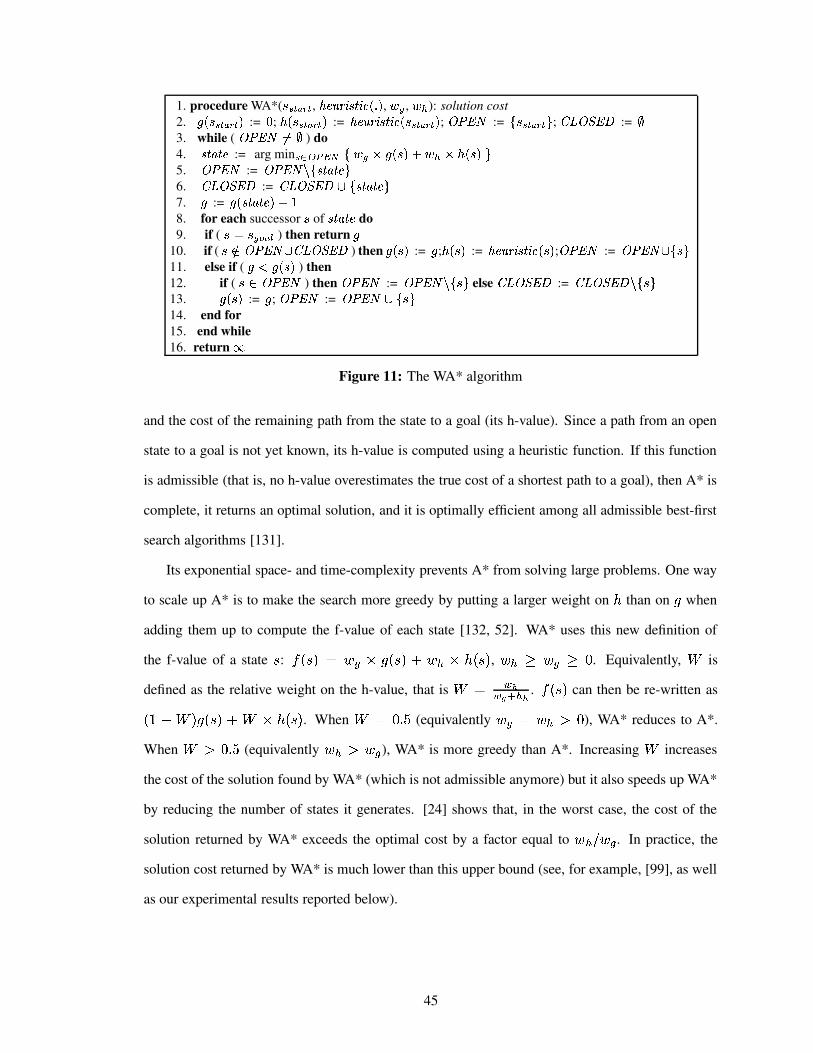
1. procedure WA*( Ö3שØZÙtÚ'Ø , Û{ÜcÝ@Þ4ßXàwá0ß�â�ã'ähå , æ2ç , æGè ): solution cost2. é�ã0Ö ×©ØZÙtÚ'Ø å := ê ; ë�ã0Ö ×�ØZÙtÚ�Ø å := Û�Ü+Ý@Þ4ßXà4á0ß�â<ã0Ö ×©ØZÙtÚ'Ø å ; ì í·îHï := ð?Ö ×©ØZÙtÚ'سñ ; ò�óGìAô{îHõ := ö3. while ( ì·í îHïÏ÷ø ö ) do4. à4á�ùQá�Ü := arg min ú¨ûaü�ý�þYÿ�ðAæ2ç�� é�ã0Ö?å�� æ6è��lë>ãjÖ?å ñ5. ì·í î ï := ì í·îHï���ð�àwá�ùQá�Ü ñ6. ò�óGìAô{îHõ := ò�ó2ì)ô@î õ��¸ð�àwá�ùQá�Ü ñ7. é := é�ã'à4á©ù3á©Ü?å��8. for each successor Ö of à4á�ùQá�Ü do9. if ( Ö ø Öbç ����� ) then return é
10. if ( Ö��� ì·í îHï��^ò�ó2ì)ô@îHõ ) then é ãjÖ?å := é ; ë>ãjÖ?å := Û�Ü+Ý@Þ4ßXà4ájß�â�ã0Öfå ; ì·í î ï := ì í·îHï��)ðQÖ ñ11. else if ( é���é ãjÖ?å ) then12. if ( Ö � ì·í îHï ) then ì í·îHï := ì·í îHï���ðQÖ ñ else òSóGì)ô@îHõ := ò�ó2ì)ô{îHõ���ðQÖ ñ13. é ãjÖ?å := é ; ì·í î ï := ì·í î ï���ð?Ö ñ14. end for15. end while16. return �
Figure 11: The WA* algorithm
and the cost of the remaining path from the state to a goal (its h-value). Since a path from an open
state to a goal is not yet known, its h-value is computed using a heuristic function. If this function
is admissible (that is, no h-value overestimates the true cost of a shortest path to a goal), then A* is
complete, it returns an optimal solution, and it is optimally efficient among all admissible best-first
search algorithms [131].
Its exponential space- and time-complexity prevents A* from solving large problems. One way
to scale up A* is to make the search more greedy by putting a larger weight on � than on � when
adding them up to compute the f-value of each state [132, 52]. WA* uses this new definition of
the f-value of a state : : �G%�:Y, ��� x ��� %�:Y, � ��� �_� %�:�, , ���9~�� x ~�m . Equivalently, is
defined as the relative weight on the h-value, that is � � �� ±"! � � . �G%�:�, can then be re-written as
%w�EÁÐ�, � %�:Y, � �Ñ� %�:Y, . When � m�P � (equivalently � x �#����| m ), WA* reduces to A*.
When |Cm�P � (equivalently �$� |%� x ), WA* is more greedy than A*. Increasing increases
the cost of the solution found by WA* (which is not admissible anymore) but it also speeds up WA*
by reducing the number of states it generates. [24] shows that, in the worst case, the cost of the
solution returned by WA* exceeds the optimal cost by a factor equal to �����&� x . In practice, the
solution cost returned by WA* is much lower than this upper bound (see, for example, [99], as well
as our experimental results reported below).
45
Figure 11 contains the pseudo-code for our implementation of WA*, which embodies the fol-
lowing assumptions: 1) there is a single goal state denoted :{xcy ucz , and 2) each operator (or action) has
a uniform cost of, say, one. These assumptions, while not essential to the behavior of WA*, make
the pseudo-code more concise.1 WA* takes as input the start state (and implicitly the domain op-
erators), a heuristic function (which associates an h-value with each state), and the weights applied
to the g- and h-values in the f-value computations (or, equivalently, a single parameter ). The
OPEN list is initialized with the start state (Line 2). Each generated state is stored in memory with
its g- and h-value. The former is computed as states are generated during the search (Lines 2&7),
while the latter is computed using the given heuristic function (Lines 2&10). The CLOSED list,
also initialized on Line 2, contains the set of expanded states. The main loop (Lines 3-15) is exe-
cuted until the OPEN list is empty, in which case there exists no solution path (Line 16), or until
the goal is generated for the first time (Line 9). During each iteration, the best state is selected in
OPEN (Line 4). It is moved from OPEN to CLOSED (Lines 5&6), since it is about to be expanded
(Lines 8-14). If a successor is newly generated, it is inserted into OPEN (Line 10). Otherwise, it
must be in either OPEN or CLOSED. In both cases, if the newly found path is shorter than the best
one found so far (Line 11), the successor is removed from its current location (Line 12) and inserted
into OPEN with its new, reduced g-value (Line 13). Otherwise, the successor is discarded.
The two extensions of WA* described in Sections 3.3 & 3.4 are alternatives to the following
two characteristics of WA*. First, WA* expands only one state per iteration. In contrast, KWA*
expands K ( � ~ � ) states per iteration. Second, WA* keeps (in OPEN) all generated states as
potential candidates for expansion. In contrast, MSC-WA* reduces the size of the set of candidates
for expansion to a small constant. The next two sections describe these two variants of WA*,
respectively.
3.3 The KWA* algorithm: Introducing diversity in WA*
WA* is a greedy version of A*. This has two implications. First, like A*, WA* is a best-first
search algorithm that always expands next the most promising node, namely an open node with the
1The pseudo-code also omits the management of back-pointers that enable the recovery of the solution path when thesearch terminates at the goal state.
46

smallest f-value. Second, since it is greedy, WA* puts more weight on the h-value than A* does, and
the more so, the closer to 1 the value of . As a result, WA* is likely to get trapped in regions of
the search space in which the h-values are misleading (namely, too low). This problem is common
among greedy search algorithms, which are attracted to local minima.
K-best-first search (KBFS) is an answer to this problem: it reduces the greediness of the search
by re-introducing a breadth-first component into best-first search [37]. The idea is to expand �nodes ( � ~�� ) at each iteration of the main loop, instead of just one as in standard best-first search.
Applied to WA*, this idea results in the KWA* algorithm.
Figure 12 contains the pseudo-code for KWA*. The only difference with WA* is that Lines 4-6
in Figure 11, in which a single most promising node is selected for expansion, are replaced with
Lines 4-10 in Figure 12, in which � most promising nodes are selected for expansion. Later (see
Lines 11-21 in Figure 12), these nodes are expanded in parallel so that the set of all their successors
is added to OPEN before the next iteration begins. This is the crucial point in order to avoid focusing
the search greedily (and often wastefully) around a local minimum.
To illustrate this point, let us consider the following example. Assume the start state has two
successors with f-values equal to 10 and 20, respectively. Note that, since we are interested in cases
with | � , the f-values are not monotonically increasing when going down the tree. Further
assume that the goal is only reachable via the second successor. Therefore, choosing the first suc-
cessor to expand next is a mistake for WA*. If the first successor is the root of a large sub-tree
whose states also have misleading h- and thus f-values, WA* keeps exploring this sub-tree until all
f-values in the OPEN list become larger than or equal to 20. This happens because WA* focuses
the search on a single successor of the start state. In contrast, when expanding the � best nodes in
OPEN (for ���"! , say), KWA* expands the start state in the first iteration. At this point, the OPEN
list contains the two successors of the start state. KWA* expands them both in the second iteration.
All their successors are added to the OPEN list. Two of them are then selected for expansion. The
difference now is that there is a chance that one of them (or both) is in the ‘good’ sub-tree, namely
the one rooted at the second successor of the start state. This is a way of adding diversity to the
search, as opposed to focusing on a single sub-tree. Of course, this diversity may be advantageous
at various levels in the search tree, not just at the start state. Generally speaking, the larger � , the
47
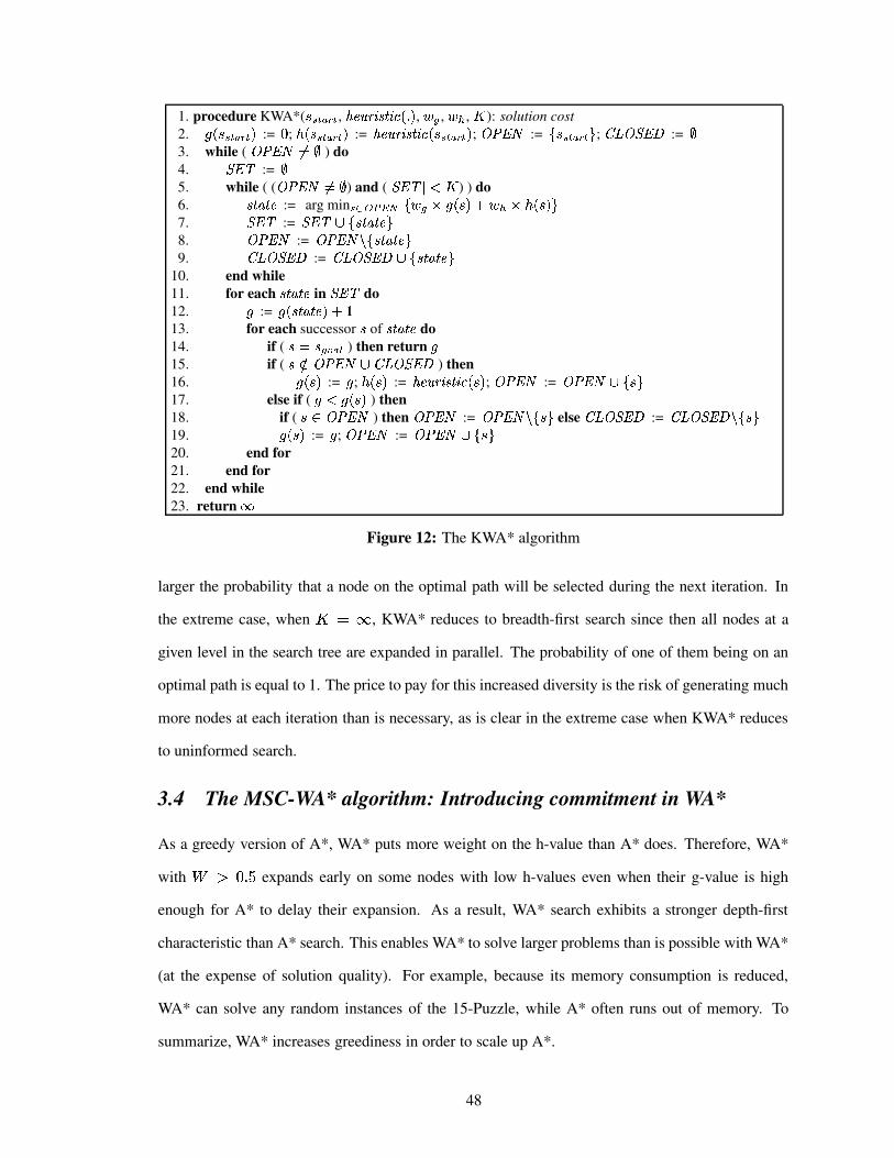
1. procedure KWA*( Ö3שØZÙtÚ'Ø , Û{ÜcÝ@Þ4ßXàwá0ß�â�ã'ähå , æ2ç , æ6è , ' ): solution cost2. é ãjÖ ×�ØZÙtÚ�Ø å := ê ; ë>ãjÖ ×�ØXÙtÚ'Ø å := Û{ÜcÝ@Þ4ßXà4ájß�â�ã0Ö ×�ØZÙtÚ�Ø å ; ì·í îHï := ðQÖ ×©ØZÙtÚ'سñ ; ò�ó2ì)ô{îHõ := ö3. while ( ì·í îHï ÷ø ö ) do4. ô@î�( := ö5. while ( ( ì·í îHïÏ÷ø ö ) and ( )hô{î�(*)+�,' ) ) do6. àwá�ùQá�Ü := arg min ú¨ûaü ý{þYÿ�ðbæ2ç�� é ãjÖ?å� æ6è��lë>ãjÖ?å ñ7. ô@î�( := ô{î�(-��ð�à4á©ù3á©Ü ñ8. ì í·îHï := ì·í îHï��Yð<à4á©ù3á©Ü ñ9. òSóGì)ô@îHõ := ò�ó2ì)ô{îHõ.��ð�à4á©ù3á©Ü ñ
10. end while11. for each à4á©ù3á©Ü in ô{î�( do12. é := é ã�à4á©ù3á©Ü?å���13. for each successor Ö of àwá�ùQá�Ü do14. if ( Ö ø Ö ç �/�0� ) then return é15. if ( Ö1�� ì·í îHï2��ò�ó2ì)ô@î õ ) then16. é ãjÖ?å := é ; ë�ã0Öfå := Û{ÜcÝ@Þ4ßXàwá0ß�â�ãjÖ?å ; ì·í îHï := ì·í îHï2�¸ð?Ö ñ17. else if ( é��Jé ãjÖ?å ) then18. if ( Ö � ì·í î ï ) then ì·í îHï := ì·í îHï��Yð?Ö ñ else ò�ó2ì)ô@î õ := òSóGì)ô@îHõ��Yð?Ö ñ19. é ãjÖ?å := é ; ì·í îHï := ì·í îHï2��ðQÖ ñ20. end for21. end for22. end while23. return �
Figure 12: The KWA* algorithm
larger the probability that a node on the optimal path will be selected during the next iteration. In
the extreme case, when � ��q , KWA* reduces to breadth-first search since then all nodes at a
given level in the search tree are expanded in parallel. The probability of one of them being on an
optimal path is equal to 1. The price to pay for this increased diversity is the risk of generating much
more nodes at each iteration than is necessary, as is clear in the extreme case when KWA* reduces
to uninformed search.
3.4 The MSC-WA* algorithm: Introducing commitment in WA*
As a greedy version of A*, WA* puts more weight on the h-value than A* does. Therefore, WA*
with |}m�P � expands early on some nodes with low h-values even when their g-value is high
enough for A* to delay their expansion. As a result, WA* search exhibits a stronger depth-first
characteristic than A* search. This enables WA* to solve larger problems than is possible with WA*
(at the expense of solution quality). For example, because its memory consumption is reduced,
WA* can solve any random instances of the 15-Puzzle, while A* often runs out of memory. To
summarize, WA* increases greediness in order to scale up A*.
48
Another way to scale up A* with a depth-first component, is to focus the search on a sub-set
of nodes in the OPEN list. This is the idea behind Multi-State Commitment (MSC) search [88].
Applied to WA*, this idea results in the MSC-WA* algorithm.
WA* keeps in OPEN the end points (that is, nodes) of all paths currently under construction.
So WA* does not commit to any region of the search space: based on the lowest f-value, WA* can
expand next any node in OPEN, even if it is very distant (in the search space) from the most recently
expanded node. WA* can jump around the state space indiscriminately among open nodes. This
is beneficial since it allows WA* 1) to stop exploring a promising region of the search space when
later expansions reveal that its h-values are misleading and 2) to restart exploration from a different
node in OPEN. Unfortunately, this “insurance” against mistakes comes at the cost of growing a
wide search front. In this sense, WA* does not make any commitment: any node in OPEN can be
expanded next if its f-value warrants it. In short, lack of commitment leads to a wide search front,
which in turn results in large memory requirements and thus poor scaling (as demonstrated by the
performance of WA* in the 35-Puzzle, see Table 9).
To address this problem, [88] introduces the notion of commitment, according to which only
a sub-set of the OPEN nodes are currently active and stored in the COMMIT list. Only one of
them can be expanded next. The other nodes in OPEN are on the RESERVE list. They are used to
refill the COMMIT list when it becomes smaller than its predefined size � . Decreasing � means
sharpening the focus of the search to a smaller sub-set of the open nodes. In turn, this introduces a
stronger depth-first search component in order to scale up the search to larger problems. Applied to
WA* this idea results in MSC-WA*.
The first difference with WA* is that the OPEN list is split into the COMMIT and RESERVE
lists. While the former plays the role of a smaller OPEN list, the latter is used as storage for
generated nodes that are not currently committed to but that the search may return to later on. This
is useful because of the second difference with WA*, namely the fact that MSC-WA* never re-
expands a node, even if a shorter path to it is later found (the designers of MSC-WA* made that
design choice because they were more interested in finding solutions quickly than in the solution
cost [88]). As a result, the COMMIT list may not be filled to capacity or may even become empty.
Figure 13 contains the pseudo-code for MSC-WA*. The algorithm takes one more parameter
49

1. procedure MSC-WA*( :436587�9:5 , ;=<?>A@CBED"F6B:G�%¨P�, , � x , ��� , � ): solution cost2. � %�:H365I7 9:5¨, := m ; � %�:H365I7 9:5¨, := ;A<J>K@"BED"F6B:G�%�:H365I7 9:5t, ; L*MONPNRQTS := M�:H36587�9:54T ;3. U�VXW=VOU�YZV := [ ; L]\�MXWAVO^ := [4. while ( L*MONPNRQTS ��_[ ) do5. D?Fa`TFb< := arg min r4£dceKf*fXg�h Mi� x �8� %�:Y, � ��� ��� %�:Y,2T6. L*MONRNPQTS := L*MONPNPQTS�j�MTD"Fa`TFb<aT7. L]\�MXWAVO^ := L]\iMXW=VO^lk�MTD"Fa`TFb<�T8. for each successor : of D"Fa`TFb< do9. if ( :�� :<xcy ucz ) then return �
10. if ( :8�7�L*MONPNPQTSmknU�VXW=VOU�YZVokpL]\iMXWAVq^ ) then11. � %�:�, := � %�D"Fa`HFb<@, � � ; � %�:Y, := ;A<J>K@"BED"F6B:Ga%�:Y, ; L*MONRNPQTS := L*MONRNPQTSrk�M�:@T12. end for13. while ( s6L*MONRNPQTS�s�|�� ) do14. D"Fa`TFb< := arg max r+£�c�eKfXfXg hJM*� x �8� %�:Y, � ��� ��� %�:�,6T15. L*MONPNRQTS := L*MONRNPQTS�j�MTD?Fa`TFb<�T16. U�VXW=VOU�YZV := U�VXW=VOU�YZVok�MTD"Fa`TFb<�T17. end while18. while ( ( s6L*MONRNPQTS�san�� ) and ( stU�VXW=VOU�YZV�s�|om ) ) do19. D"Fa`TFb< := arg min r+£Tu�vKw?vAuZxyv Mi� x �8� %�:Y, � ��� ��� %�:Y,2T20. U�VXW=VOU�YZV := U�VXW=VOU�YZV�j�MTD?Fa`TFb<�T21. L*MONPNRQTS := L*MONRNPQTS�k�MTD?Fa`TFb<�T22. end while23. end while24. return q
Figure 13: The MSC-WA* algorithm
50
than WA*, namely the size � of the COMMIT list. The COMMIT list is initialized to the start
state, while the RESERVE and CLOSED lists are initially empty (Lines 2&3). Then the main loop
(Lines 4-23) is executed until COMMIT is empty (in which case there is no solution, Line 24) or
until the goal is generated for the first time (Line 9). At each iteration, the best node in COMMIT
is selected for expansion and moved to the CLOSED list (Lines 5-7). Every newly generated node
is added to the COMMIT list (Lines 10-11). If the COMMIT list is too large, the least promising
nodes are moved to the RESERVE list (Lines 13-17). but if the COMMIT list not full, the most
promising nodes in the RESERVE (if any) are used to fill it up (Lines 18-22).
To illustrate the behavior of MSC-WA*, we now consider two extreme cases. When ����� ,MSC-WA* performs a greedy search. Starting with the start node, the current node is repeatedly
removed from COMMIT (which is now empty) and expanded. All its successors are added into
COMMIT. All but the most promising ones are immediately moved to the RESERVE. At the end of
each iteration, the COMMIT list only contains the best successor of the current node. This depth-
first search stops when the goal is reached or when a dead-end is reached (either because there exists
a dead-end in the search space or because no new state is reachable from the current one). In the
latter case, the search is restarted from the best state in the RESERVE.
When ����q , the COMMIT list never fills up and the RESERVE list remains empty. As a
result, COMMIT behaves like the original OPEN list. In this case, MSC-WA* reduces to a version
of WA* that never re-expands a node. When � ranges from 2 to infinity, MSC-WA* becomes less
and less focused and resembles more and more best-first search with no commitment. MSC-WA*
grows a search tree in which at most � leaves are active at any time. Some children of the just-
expanded node may be preferred over nodes in the RESERVE with smaller f-values. This sharper
focus explains how MSC-WA* is able to scale up greedy best-first search to larger domains than
WA* can handle.
3.5 The MSC-KWA* algorithm: Combining diversity and commitment
In this section, we first contrast the effects of diversity and commitment on the performance of
best-first search. Since these ideas are orthogonal, we then show how to combine them into a new
algorithm (MSC-KWA*) that scales up to larger problems than is possible with diversity (KWA*)
51

or commitment (MSC-WA*) alone.
3.5.1 Comparing the behaviors of KWA* and MSC-WA*
When assessing the behavior of our heuristic search algorithms, we use four standard performance
measures, namely memory consumption, solution cost, search effort, and runtime. Since our pri-
mary objective is to scale up best-first search to larger domains, and since the memory usage is the
main obstacle in this respect, the memory consumption is our primary focus. When the available
memory is enough for an algorithm to terminate successfully on all instances, the solution cost is
our secondary performance measure. This preference (over search effort and runtime) is justified
by the facts that:
k The search effort (that is, the number of generated nodes) is strongly correlated with the
memory consumption, as our empirical results have demonstrated for all the algorithms under
consideration.
k The runtime is on the order of seconds since the memory typically available on current PC’s
is quickly filled up by best-first search algorithms such as variants of WA*.2
In summary, our comparison focuses primarily on the functional relationship between the memory
consumption and the solution cost.
In this sub-section, we use a preview of our empirical results in the�
-puzzle to compare the
behaviors of KWA* and MSC-WA*. Since each of the KWA* and MSC-WA* algorithms has two
parameters (namely, and either � or � ), our full empirical results are structured as two sets of
memory-cost functions parameterized on each parameter (see Section 3.6). Here in contrast, we
abstract away the influence of these parameters and use graphs that associate with each solution
cost the minimum memory consumption over all settings of the parameters. We thus obtain a single
curve per algorithm. In essence, we consider an idealized situation in which an oracle tells us the
parameter settings that minimize the memory consumption for a given solution cost. The resulting
curves are shown in Figure 14 for the�
-Puzzle with� �_z�(3� � (c!�Ç (cÌ � .
We observe the following trends:
2In this chapter, we do not consider memory-bounded algorithms (e.g., [96, 19, 143, 86, 177]) because, even thoughthey do not run out of memory, they exhibit unacceptably large runtimes due to their node-regeneration overhead.
52

1000
10 20 30 40 50 60 70 80 90 100
Number of Stored Nodes (log scale)
Solution Cost
WA*KWA*
MSC-WA*
a) 8-Puzzle
1000
10000
100000
1e+06
100
Number of Stored Nodes (log scale)
Solution Cost (log scale)
WA*KWA*
MSC-WA*
b) 15-Puzzle
100000
1e+06
100 1000
Number of Stored Nodes (log scale)
Solution Cost (log scale)
WA*KWA*
MSC-WA*
c) 24-Puzzle
1e+06
1000
Number of Stored Nodes (log scale)
Solution Cost (log scale)
KWA*MSC-WA*
d) 35-Puzzle
Figure 14: Performance comparison: WA*, KWA*, and MSC-WA* in the�
-Puzzle
k The larger the domain, the more KWA* reduces the memory consumption (for a given solu-
tion cost) over WA*. While there is no significant improvement in the 8-Puzzle, the reduction
is significant in the 15-Puzzle and even larger (about an order of magnitude) in the 24-Puzzle.
Because of this effect, KWA* is able to find shorter solutions than WA* in both the 15- and
24-Puzzle within the available memory. In other words, KWA* enlarges the range of reach-
able solution costs toward the small end (that is, toward the left in the figures) while reducing
the memory consumption (that is, a shift toward the bottom in the figures). Because of its
reduced memory consumption, KWA*, unlike WA*, is able to solve the 35-Puzzle.
k While MSC-WA* does not improve over the memory consumption of WA* (over the range of
solution costs obtainable by WA*), its main advantage, from our perspective, is that it enlarges
53
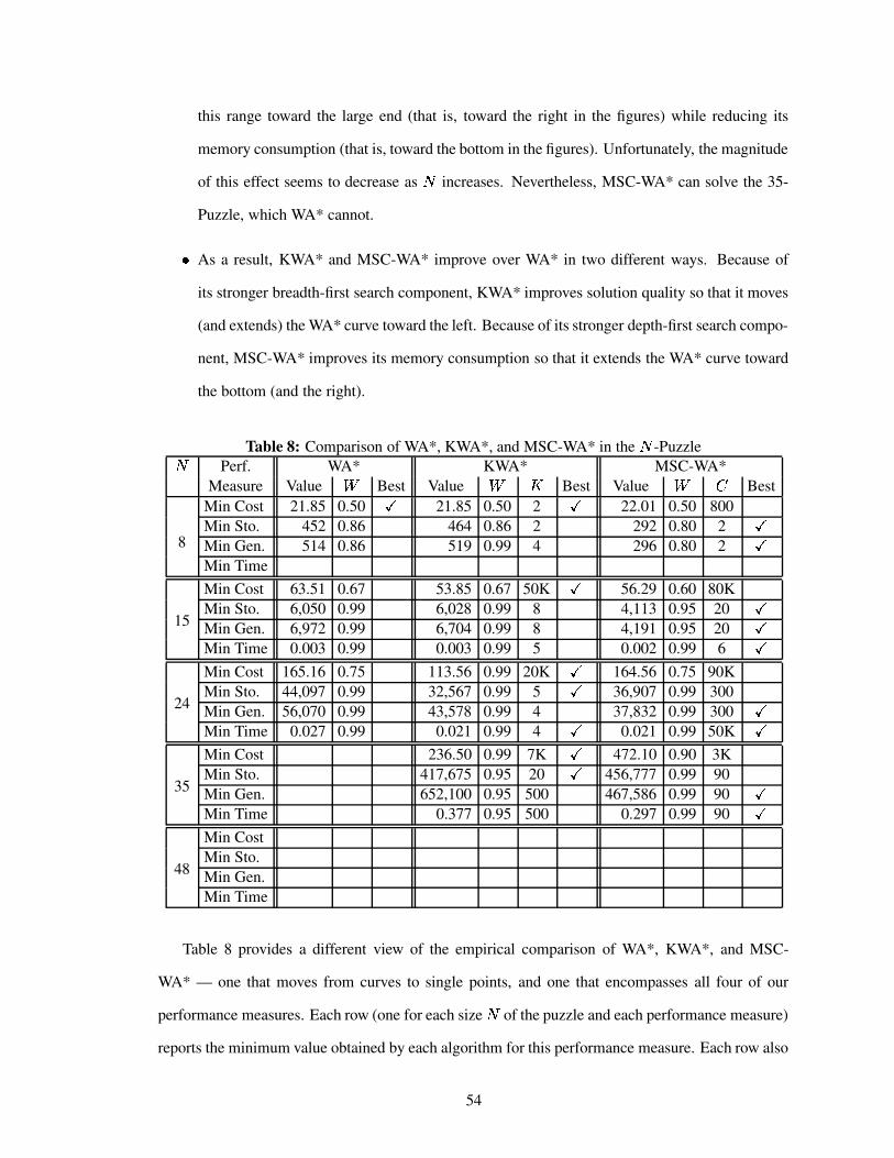
this range toward the large end (that is, toward the right in the figures) while reducing its
memory consumption (that is, toward the bottom in the figures). Unfortunately, the magnitude
of this effect seems to decrease as�
increases. Nevertheless, MSC-WA* can solve the 35-
Puzzle, which WA* cannot.
k As a result, KWA* and MSC-WA* improve over WA* in two different ways. Because of
its stronger breadth-first search component, KWA* improves solution quality so that it moves
(and extends) the WA* curve toward the left. Because of its stronger depth-first search compo-
nent, MSC-WA* improves its memory consumption so that it extends the WA* curve toward
the bottom (and the right).
Table 8: Comparison of WA*, KWA*, and MSC-WA* in the�
-Puzzle�Perf. WA* KWA* MSC-WA*
Measure Value Best Value � Best Value � Best
8
Min Cost 21.85 0.50 { 21.85 0.50 2 { 22.01 0.50 800Min Sto. 452 0.86 464 0.86 2 292 0.80 2 {Min Gen. 514 0.86 519 0.99 4 296 0.80 2 {Min Time
15
Min Cost 63.51 0.67 53.85 0.67 50K { 56.29 0.60 80KMin Sto. 6,050 0.99 6,028 0.99 8 4,113 0.95 20 {Min Gen. 6,972 0.99 6,704 0.99 8 4,191 0.95 20 {Min Time 0.003 0.99 0.003 0.99 5 0.002 0.99 6 {
24
Min Cost 165.16 0.75 113.56 0.99 20K { 164.56 0.75 90KMin Sto. 44,097 0.99 32,567 0.99 5 { 36,907 0.99 300Min Gen. 56,070 0.99 43,578 0.99 4 37,832 0.99 300 {Min Time 0.027 0.99 0.021 0.99 4 { 0.021 0.99 50K {
35
Min Cost 236.50 0.99 7K { 472.10 0.90 3KMin Sto. 417,675 0.95 20 { 456,777 0.99 90Min Gen. 652,100 0.95 500 467,586 0.99 90 {Min Time 0.377 0.95 500 0.297 0.99 90 {
48
Min CostMin Sto.Min Gen.Min Time
Table 8 provides a different view of the empirical comparison of WA*, KWA*, and MSC-
WA* — one that moves from curves to single points, and one that encompasses all four of our
performance measures. Each row (one for each size�
of the puzzle and each performance measure)
reports the minimum value obtained by each algorithm for this performance measure. Each row also
54

reports, for each algorithm, one parameter setting with which the algorithm reaches the minimum
value of this performance measure. Finally, a check mark indicates that the algorithm is within one
percent of the minimum value reported in the row. A check mark thus means that this algorithm is
the best according to the performance measure and for this puzzle size. Empty cells indicate that
the algorithm does not solve all instances of this�
-Puzzle (except for the 8-Puzzle, in which case
runtimes are not reported because they are insignificant).
First, both KWA* and MSC-WA* improve on WA* since only they can solve all instances of
the 35-Puzzle. Second, because of its breadth-first search component, KWA* is always the best
algorithm according to solution quality. Third, because of its depth-first (greedy) component, MSC-
WA* is always the best algorithm according to the search effort (number of generated nodes) and
the runtime. Fourth, both KWA* and MSC-WA* beat WA* according to the memory consumption
(number of stored nodes). However, no algorithm consistently beats the other in this dimension.
Finally, none of the algorithms is able to solve all instances of the 48-Puzzle in our empirical setup.
3.5.2 The MSC-KWA* algorithm
Our preview of results in the�
-Puzzle suggests that KWA* and MSC-WA* have distinct advantages
over WA*. It is natural to wonder whether these advantages can be cumulated by combining the
concepts of diversity and commitment in order to scale up to even larger domains, such as the
48-Puzzle. We now turn to this question.
By forcing the search to commit to a sub-set of the OPEN list (namely the COMMIT list),
MSC-WA* uses COMMIT in the role of OPEN (while RESERVE is only used to refill COMMIT
when necessary). As a result, MSC-WA* is more focused than WA* and is thus as likely (or even
more) to be led by misleading heuristic values into goal-free regions of the search space. One way
to alleviate this problem is to add diversity to the MSC-WA* search. We propose to introduce into
MSC-WA* the mechanism used by KWA*: instead of expanding the best node in COMMIT at each
iteration, we propose to expand a sub-set of the best � �"� nodes in COMMIT in parallel at each
iteration. We call the resulting algorithm MSC-KWA*.
Figure 15 contains the pseudo-code for MSC-KWA*. It takes three parameters, namely , � ,
and � . After initializing the COMMIT and RESERVE lists identically to MSC-WA* (Lines 2 & 3),
55
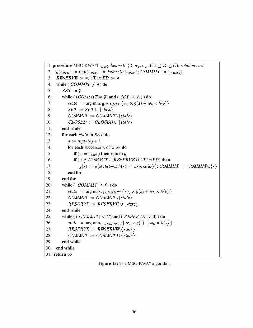
1. procedure MSC-KWA*( :436587�9:5 , ;A<?>A@"B|D?F6B6Ga%¨P�, , � x , ��� , � , �ª�o� �9� ): solution cost2. � %�:H365I7 9:5¨, := m ; � %�:H365I7 9:5¨, := ;A<J>K@"BED"F6B:G�%�:H365I7 9:5t, ; L*MONPNRQTS := M�:H36587�9:54T ;3. U�VXW=VOU�YZV := [ ; L]\�MXWAVO^ := [4. while ( L*MONPNRQTS ��_[ ) do5. W=V�S := [6. while ( ( L*MONRNPQTS���2[ ) and ( s}W=V�S~sano� ) ) do7. D"Fa`HFb< := arg min r+£�c�eKfXfXg hJM�� x �8� %�:Y, � ��� ��� %�:Y,cT8. WAV1S := W=V�Smk�MTD?Fa`TFb<aT9. L*MONPNRQTS := L*MONRNPQTS�j�MTD?Fa`TFb<�T
10. L]\iMXWAVq^ := L]\�MXWAVO^�k�MTD"Fa`HFb<�T11. end while12. for each D"Fa`TFb< in WAV1S do13. � := � %�D"Fa`TFb<{, � �14. for each successor : of D?Fa`TFb< do15. if ( :À�":�xcy ucz ) then return �16. if ( : �7oL*MONRNPQTSmk�U�VXWAVqU�YZV�k.L]\�MXWAVO^ ) then17. � %�:Y, := � %�D"Fa`TFb<@, � � ; � %�:Y, := ;A<J>A@CBED"F6B:G�%�:Y, ; L*MONPNPQTS := L*MONPNRQTS�k¾M�:{T18. end for19. end for20. while ( s6L*MONRNPQTS�s�|�� ) do21. D"Fa`TFb< := arg max r+£�c�eKfXfXg hJM*� x �8� %�:Y, � ��� ��� %�:�,6T22. L*MONPNRQTS := L*MONRNPQTS�j�MTD?Fa`TFb<�T23. U�VXW=VOU�YZV := U�VXW=VOU�YZVok�MTD"Fa`TFb<�T24. end while25. while ( ( s6L*MONRNPQTS�san�� ) and ( stU�VXW=VOU�YZV�s�|om ) ) do26. D"Fa`TFb< := arg min r+£Tu�vKw?vAuZxyv Mi� x �8� %�:Y, � ��� ��� %�:Y,2T27. U�VXW=VOU�YZV := U�VXW=VOU�YZV�j�MTD?Fa`TFb<�T28. L*MONPNRQTS := L*MONRNPQTS�k�MTD?Fa`TFb<�T29. end while30. end while31. return q
Figure 15: The MSC-KWA* algorithm
56
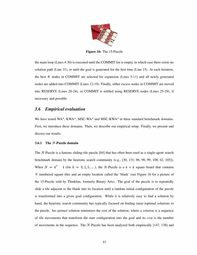
Figure 16: The 15-Puzzle
the main loop (Lines 4-30) is executed until the COMMIT list is empty, in which case there exists no
solution path (Line 31), or until the goal is generated for the first time (Line 15). At each iteration,
the best � nodes in COMMIT are selected for expansion (Lines 5-11) and all newly generated
nodes are added into COMMIT (Lines 12-19). Finally, either excess nodes in COMMIT are moved
into RESERVE (Lines 20-24), or COMMIT is refilled using RESERVE nodes (Lines 25-29), if
necessary and possible.
3.6 Empirical evaluation
We have tested WA*, KWA*, MSC-WA* and MSC-KWA* in three standard benchmark domains.
First, we introduce these domains. Then, we describe our empirical setup. Finally, we present and
discuss our results.
3.6.1 The�
-Puzzle domain
The�
-Puzzle is a famous sliding-tile puzzle [84] that has often been used as a single-agent search
benchmark domain by the heuristic search community (e.g., [30, 131, 96, 98, 99, 108, 42, 105]).
When� ��Ë 5 Á�� (for ËK��Ì�(4Ç ( � (QPQPQP ), the
�-Puzzle is a Ë � Ë square board that contains
�numbered square tiles and an empty location called the ‘blank’ (see Figure 16 for a picture of
the 15-Puzzle sold by Thinkfun, formerly Binary Arts). The goal of the puzzle is to repeatedly
slide a tile adjacent to the blank into its location until a random initial configuration of the puzzle
is transformed into a given goal configuration. While it is relatively easy to find a solution by
hand, the heuristic search community has typically focused on finding (near-)optimal solutions to
the puzzle. An optimal solution minimizes the cost of the solution, where a solution is a sequence
of tile movements that transform the start configuration into the goal and its cost is the number
of movements in the sequence. The�
-Puzzle has been analyzed both empirically [147, 138] and
57

theoretically [137]. The latter reference contains a proof that optimally solving the�
-Puzzle is
NP-hard.
In general, the size of the state space for the�
-Puzzle, that is the number of states reachable
from the start state, is equal to % � � �<,b��Y! . For the 8-Puzzle, this size is relatively small so that the
whole state space can fit into memory and non-heuristic search techniques (e.g., breadth-first search)
can solve it optimally in no time. The 15-Puzzle was first solved optimally using the IDA* algorithm
[96] (a linear-space heuristic search algorithm) with the Manhattan distance heuristic function. The
Manhattan distance is the sum, over all tiles, of the tile’s distance from its current location to its
goal location in both the horizontal and vertical directions. Since each tile must move at least that
many times to reach its goal position and each sliding action only moves one tile, the Manhattan
distance (henceforth referred to as ‘MD’) is an admissible heuristic for the�
-Puzzle. This heuristic
was also used to solve larger versions of the puzzle (that is, Ë |ÂÇ ) with real-time search algorithms
[98].
An enhancement to MD called the linear conflict heuristic (LC) increases the pruning power
of MD and reduces the number of generated states by a factor of 8 in the 15-Puzzle [58]. Due to
the additional overhead involved in computing the heuristic value for each node, LC yields a 5-fold
runtime speedup over MD [108]. However, only when LC was extended to a more general way
of generating admissible heuristics (called pattern databases [22, 23]) was the 24-Puzzle solved
optimally for the first time [108]. In a later paper [105], it is estimated (based on analytical results
developed in [107]) that optimally solving a random instance of the 24-Puzzle with MD would take
on average about 50,000 years. In contrast, the average solving time with pattern databases is 2 days
(with a rather large variance).
Despite impressive recent improvements in the pattern database technology (e.g., [69, 36, 38]),
the performance of admissible search in the 35-Puzzle can only be predicted (e.g., [36]) and it is
expected that this puzzle will not be solved optimally in the near future. For this reason, and because
it is often preferable to obtain suboptimal solutions fast than to wait too long for an optimal one,
suboptimal search is an active area of research. In this context also, the�
-Puzzle is often used both
for testing domain-dependent search and learning algorithms [42] and as a benchmark for domain-
independent suboptimal search [136, 98, 88, 37].
58

Figure 17: The 4-peg Towers of Hanoi
In short, the�
-Puzzle has been and remains a standard tool for measuring progress in both
optimal and suboptimal heuristic search algorithms (and heuristic functions). In this work, we use
it to measure the performance of WA* and some of its recent variants. In our experiments using
MD, WA* can only solve all random instances of the�
-puzzle for�
up to and including 24. Both
KWA* and MSC-WA* scale up to the 35-Puzzle but run out of memory on some random instances
of the 48-Puzzle. Finally, the combination of KWA* and MSC-WA* (MSC-KWA*) does scale up
to the 48-Puzzle.
3.6.2 The 4-peg Towers of Hanoi domain
The Towers of Hanoi problem is an old and famous problem [118, 32, 45, 160] that has
been used and studied by mathematicians, and cognitive and computer scientists alike (e.g.,
[157, 62, 168, 127, 9, 8, 141, 117, 26, 64, 5, 145, 36]). In addition to being a worthwhile object of
mathematical study in its own right, the Towers of Hanoi problem is a useful tool for demonstrating
the behavior of recursive algorithms, as well as a benchmark task for the study (both physiological
and computational) of cognitive processes.
A problem instance is characterized by the number [�~ÐÌ of pegs (or towers), the number � ~K�of disks, and the initial location (that is, peg) of each disk. No two disks have the same diameter.
One peg is identified as the destination peg. The objective is to find a sequence of moves that gets
all of the disks stacked on the destination peg. A move consists in moving a single disk from the
top of a stack on any peg onto any other peg. The only constraint is that a larger disk can never lie
on top of a smaller disk.
Computational studies of the Towers of Hanoi problem typically focus on the length of the
solution sequence. The most commonly studied class of instances has [���Ì . In this case, the
optimal solution cost (that is, the length of a shortest sequence) is exponential in � in the worst
59
case. This class of problems is considered solved since there is a known algorithm that is guaranteed
to find optimal solutions. In contrast, the case [���Ç (called Reve’s puzzle) is still open. Existing
algorithms are only conjectured to be optimal [9, 8, 145]. Since Reve’s puzzle is becoming popular
in the heuristic search community [103, 104, 38, 36], we use it as one of our benchmarks (see
Figure 17 for a picture of a 4-peg Towers of Hanoi set).
Since each of the � disks can be on any of the four pegs and there is only one way to stack
a given set of disks on a peg, the � -disk Reve’s puzzle contains Ç�� distinct states. A simple
memoryless heuristic for this puzzle is the number of misplaced disks, where a disk is misplaced
when it is not on the destination peg. This heuristic is clearly admissible since each misplaced disk
must move at least once. A slightly more informed and still admissible heuristic is the so-called
infinite-peg heuristic [36]. It is obtained by solving optimally a relaxed version of Reve’s puzzle,
namely one in which there are infinitely many pegs (or equivalently � � Ç pegs). Unfortunately,
both of these heuristics are rather poorly informed. Therefore, we use a pattern database as our
heuristic function. In [103, 104, 38, 36], a pattern database for a Towers of Hanoi problem with
� disks is a lookup table of the minimum costs of solving all possible configurations of� ���
disks. This heuristic is clearly admissible and takes into account some of the disk interactions that
memoryless heuristics ignore. The larger�, the more interactions are accounted for and the more
informed the heuristic. In the extreme case, where� ��� , the heuristic is perfectly informed. The
largest instances solved optimally by heuristic search with pattern databases have ������z [38]3.
We set ���O!@! and� � �3Ì . The first value was chosen in order to demonstrate the advantage of
suboptimal searches for scaling up. The second was chosen based on our available memory: Our
13-disk pattern database uses 64Mbytes of memory. The rest of the available memory is used to
store search nodes.
3In [38], such large instances of the Towers of Hanoi are solved with enhancements to the simple idea of a patterndatabases, namely additive pattern databases and compressed pattern databases. Our heuristic does not take advantage ofthese enhancements. Note that [104] solves optimally one instance with ���,�c� using breadth-first search and externalmemory.
60
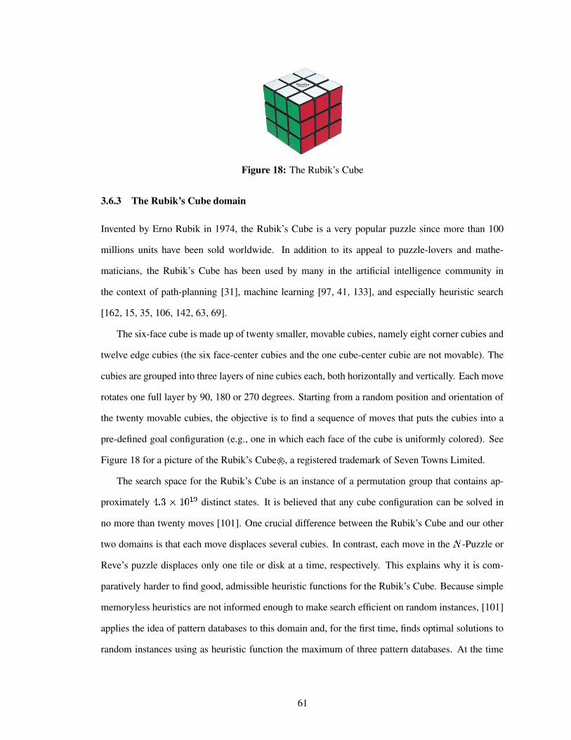
Figure 18: The Rubik’s Cube
3.6.3 The Rubik’s Cube domain
Invented by Erno Rubik in 1974, the Rubik’s Cube is a very popular puzzle since more than 100
millions units have been sold worldwide. In addition to its appeal to puzzle-lovers and mathe-
maticians, the Rubik’s Cube has been used by many in the artificial intelligence community in
the context of path-planning [31], machine learning [97, 41, 133], and especially heuristic search
[162, 15, 35, 106, 142, 63, 69].
The six-face cube is made up of twenty smaller, movable cubies, namely eight corner cubies and
twelve edge cubies (the six face-center cubies and the one cube-center cubie are not movable). The
cubies are grouped into three layers of nine cubies each, both horizontally and vertically. Each move
rotates one full layer by 90, 180 or 270 degrees. Starting from a random position and orientation of
the twenty movable cubies, the objective is to find a sequence of moves that puts the cubies into a
pre-defined goal configuration (e.g., one in which each face of the cube is uniformly colored). See
Figure 18 for a picture of the Rubik’s Cube R� , a registered trademark of Seven Towns Limited.
The search space for the Rubik’s Cube is an instance of a permutation group that contains ap-
proximately Ç P Ì � �Qm 1b� distinct states. It is believed that any cube configuration can be solved in
no more than twenty moves [101]. One crucial difference between the Rubik’s Cube and our other
two domains is that each move displaces several cubies. In contrast, each move in the�
-Puzzle or
Reve’s puzzle displaces only one tile or disk at a time, respectively. This explains why it is com-
paratively harder to find good, admissible heuristic functions for the Rubik’s Cube. Because simple
memoryless heuristics are not informed enough to make search efficient on random instances, [101]
applies the idea of pattern databases to this domain and, for the first time, finds optimal solutions to
random instances using as heuristic function the maximum of three pattern databases. At the time
61

of publication, the average runtime was on the order of two days (with a large variance). As the size
of RAM increases, larger pattern databases can be used, yielding more informed heuristic functions
and reduced runtimes. In our experiments, we use Korf’s heuristic function, and any additional
available RAM is used to store the generated nodes needed by our variants of WA*.
3.6.4 Empirical setup
Problem instances. In the�
-Puzzle, we vary Ë from 3 to 7 (recall that� � Ë 5 Á®� ). In each case,
the goal state is the puzzle configuration in which the blank is in the upper left corner of the board
and the tiles are positioned in increasing order of their number (1 through�
) from left to right
within a row, from the top row down. Start states are randomly selected among the set the states
reachable from the goal. Due to timing considerations, we choose a random number of problem
instances (each characterized only by the start state) equal to 1000 and 100 for the 8- and 15-Puzzle,
respectively.4 For larger puzzles, we use 50 random instances in each case (� � � (c�(b� ).5
In the 4-peg Towers of Hanoi problem, we set � equal to 22 and�
equal to 13. The goal state
has all disks stacked up on an arbitrary peg. Fifty initial states are selected by randomly selecting a
peg as the starting position for each disk.
In the Rubik’s Cube problem, the goal state is the original configuration of the cube. Fifty initial
states are obtained by performing 500-long sequences of random moves starting in the goal state.
Implementation details. Our implementations of the WA* variants described in this chapter share
the following features.6
k They all use the same data structures for packed states and the same hashing scheme in each
domain.
k They all use the same successor-generator function which determines the systematic (that is,
non-random) order in which applicable moves are considered during expansion.
k They all prune (that is, do not generate) the successor of a node that is identical to the parent
of the node in the search tree. This simply eliminates cycles of length equal to two whose
4The 100 random instances used in the 15-Puzzle are the standard set first used in [96].5The 50 random instances used in the 24-Puzzle are the first 50 instances in the 100-long set first used in [37].6Our code for all variants of WA* results from modifications to the WA* code graciously sent to us by Richard Korf.
62

existence results from the fact that each move in the puzzle is reversible (that is, the state-
space is really an undirected graph). In addition, the same disk (layer) cannot be moved
twice in a row in the Towers of Hanoi problem (Rubik’s Cube) since the state resulting from
the sequence of two such moves can be reached in a single move. Finally in the Rubik’s
Cube, opposite faces are arbitrarily ordered (pairwise) and successive moves of opposite faces
are forced to follow this order so that redundant, commutative sequences of two moves are
avoided. These constraints applied during node expansion are standard, domain-dependent
ways of reducing the branching factors of each domain to make search as efficient as possible.
k They share the same termination condition, since they all stop as soon as the goal state is
generated for the first time.
Our experiments in the�
-Puzzle (in the Rubik’s Cube and Towers of Hanoi, respectively) were
performed on a Pentium-IV PC clocked at a 2.2 GHz (on a Pentium-III PC clocked at 1.4 GHz,
respectively) and with enough memory to store a few million nodes. This number of stored nodes is
the size of our hash table. The timings reported below always exclude the timings of initializations
(of the hash table, OPEN lists, etc.) since these are identical across instances and variants of WA*.
Runtimes are always for the search phase itself.
Performance measures. All algorithms are evaluated according to the following performance mea-
sures:
k The cost (that is, the path length) of the solution found,
k the number of nodes generated, which is a machine-independent measure of the search effort,
k the actual runtime (in seconds) of the search, and
k the number of nodes stored, which is a measure of memory consumption.
There are only two reasons why an algorithm terminates: either it has generated the goal or it has run
out of memory. Except where noted, all of our averages are computed for experimental conditions
in which all instances are solved within the memory constraints.
63

3.6.5 Empirical results in the�
-Puzzle domain
3.6.5.1 Empirical evaluation of WA* in the�
-Puzzle
Figure 19 summarizes the performance of WA* on the 8-, 15-, and 24-Puzzle. It contains six
sub-figures. Each of the first four sub-figures (a through d) plots one of our selected performance
measures against values of . We use the following values of ; 0.50, 0.56, 0.60, 0.67, 0.75,
0.80, 0,86,0.90, 0.95, 0.99.7 Only for the 8-Puzzle do we omit the runtime plot since WA* (and
all of its variants) are too fast for the runtimes to be significant. The last two sub-figures (e & f)
plot the memory usage and runtime as a function of the solution cost, respectively. Note that the
plot of the search effort as a function of the solution cost is omitted since, in all cases, it would be
very similar to sub-figure f (because, as sub-figures b & d demonstrate, the actual runtime is very
strongly correlated with the search effort as measured by the number of generated nodes).
Our results with WA* do not contain any surprises and reproduce the trends exhibited by earlier
studies (e.g., [99] and [37] for the 15-Puzzle and 24-Puzzle, respectively). Since the performance
of WA* constitutes our baseline for this research, we have decided to include these results, which
we now briefly describe. We observe the following general trends:
k The solution cost increases with (sub-figure a). As expected, making WA* more greedy
leads to a degradation in solution quality. Furthermore, as observed in earlier studies, the
degraded solution quality, measured as a multiplicative factor of the optimal solution cost,
is much smaller than the theoretical upper bound of [24]. For example in the 15-Puzzle,
where the known average optimal cost is 53.05 [96], WA* degrades solution quality by a
factor smaller than 3 when � �� ± ���T� (the average solution cost corresponding to the top-
rightmost point of the 15-Puzzle curve in Figure 19a is 145.27).
k The search effort decreases as increases (sub-figures b & d). As expected, making WA*
more greedy leads to a significant speedup. For example in the 15-Puzzle, we observe an
order of magnitude speedup between the top-leftmost and bottom-rightmost ends of the curve
7These values of � were chosen 1) to be approximately evenly distributed over the [0.5, 1] interval and 2) to cor-respond to small, relatively prime integer values of � ± and � � . These values, listed in Table 9, are a strict sub-set ofthose used in [99, 37]. The only reason for not using all of their values for � was the considerable cumulated runtimesinvolved (on the order of days) in running all variants of WA* on 50 to 1000 instances with various values for � , � aswell as values for � (see KBFS) and the size of the commitment list (see MSC-WA*).
64

50
100
150
200
250
300
350
0.5 0.6 0.7 0.8 0.9 1
Solution Cost
Relative Weight on H-values
WA*
a) Solution cost versus
0.001
0.01
0.1
1
0.5 0.6 0.7 0.8 0.9 1
Time in Seconds (log scale)
Relative Weight on H-values
24-Puzzle15-Puzzle
b) Runtime versus
1000
10000
100000
1e+06
0.5 0.6 0.7 0.8 0.9 1
Number of Stored Nodes (log scale)
Relative Weight on H-values
24-Puzzle15-Puzzle8-Puzzle
c) Memory usage versus
1000
10000
100000
1e+06
0.5 0.6 0.7 0.8 0.9 1
Number of Generated Nodes (log scale)
Relative Weight on H-values
24-Puzzle15-Puzzle8-Puzzle
d) Search effort versus
1000
10000
100000
1e+06
0 50 100 150 200 250 300 350
Number of Stored (log scale)
Solution Cost
24-Puzzle15-Puzzle8-Puzzle
e) Memory usage versus solution cost
0
0.1
0.2
0.3
0.4
0.5
0.6
0 50 100 150 200 250 300 350
Time in Seconds
Solution Cost
24-Puzzle15-Puzzle
f) Runtime versus solution cost
Figure 19: Performance of WA* in the�
-Puzzle with varying
65

in Figure 19b. As a multiplicative factor, this speedup is thus larger than the degradation in
solution quality.8 This confirms that WA* is an effective way to trade off solution quality for
runtime (or, equivalently, search effort). This trade-off is plotted in sub-figure e.
k The memory usage decreases as increases (sub-figure c). This is crucial from our point of
view, since we are interested in scaling up these algorithms to larger problems. Again, this
is not surprising: the memory consumption is proportional to the number of stored nodes,
which itself is strongly correlated with the number of generated nodes (since they are stored).
The resulting trade-off between solution cost and memory usage is plotted in sub-figure e.
Furthermore, while WA* does regenerate some nodes (see Lines 11 through 13 in Figure 11),
these represent a small percentage of the total number of node generations, as can be seen by
comparing sub-figures c and d. Each curve in sub-figure c is similarly shaped, but slightly
lower, than that in sub-figure d.
Finally, as�
increases, the range of values for which WA* solves all instances shrinks (and
the curves are increasingly truncated on their left side in Figure 19). The 35-Puzzle is the smallest
puzzle for which WA* cannot solve all random instances, even with values of close to 1. Since
WA* solves a different sub-set of the test instances for different values of , as suggested by the
last column in Table 9, it is not meaningful to use the other numbers in the table in order to study
the trade-offs observed in the smaller puzzles.
3.6.5.2 Empirical evaluation of KWA* in the�
-Puzzle
Figures 89 through 94 (see Appendix B.1) show the performance of KWA* in the 8-, 15-, and 24-
Puzzle domains. Figures 20 and 21 summarize the performance of KWA* in the 35-Puzzle domain
(these figures demonstrate the better scaling of KWA* over WA* and are thus included in the main
text below).
Since KWA* adds one more parameter (namely � ) to already used by WA*, we vary each
8Furthermore, note that the top-leftmost point in the figure does not correspond to WA*. The curve is truncated tothe left because, for smaller values of � including ��� ��� �b� , WA* runs out of memory. A* (equivalently, WA* with������ �c� ) would in fact be much slower. For a suggestive comparison, the curve is truncated at ������ �?� where thenumber of nodes generated is equal to 78,870 (see Figure 19d). IDA*, on the other hand, generates 363,028,090 nodes inorder to guarantee optimal solutions [99]. Even allowing for the duplicated effort incurred by IDA* over WA*, this is atleast 4 orders of magnitude worse than the 6,972 nodes generated by WA* when ��� ��� �"� (see Figure 19d).
66
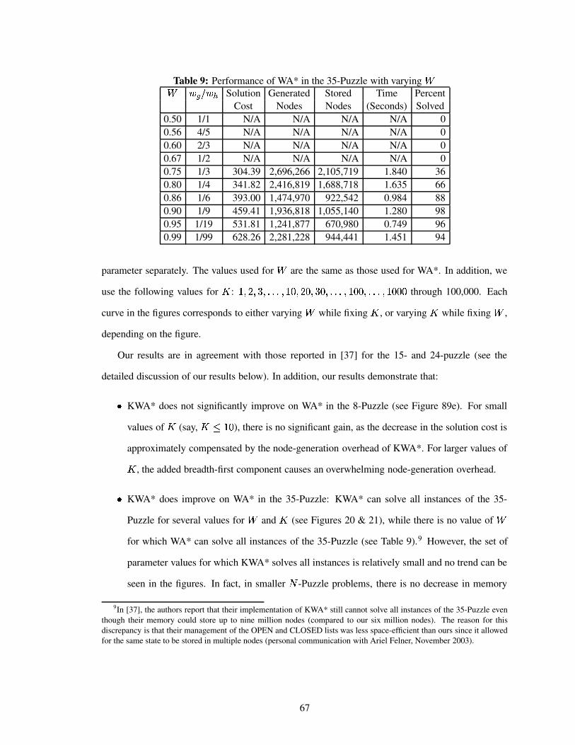
Table 9: Performance of WA* in the 35-Puzzle with varying � x �&��� Solution Generated Stored Time Percent
Cost Nodes Nodes (Seconds) Solved0.50 1/1 N/A N/A N/A N/A 00.56 4/5 N/A N/A N/A N/A 00.60 2/3 N/A N/A N/A N/A 00.67 1/2 N/A N/A N/A N/A 00.75 1/3 304.39 2,696,266 2,105,719 1.840 360.80 1/4 341.82 2,416,819 1,688,718 1.635 660.86 1/6 393.00 1,474,970 922,542 0.984 880.90 1/9 459.41 1,936,818 1,055,140 1.280 980.95 1/19 531.81 1,241,877 670,980 0.749 960.99 1/99 628.26 2,281,228 944,441 1.451 94
parameter separately. The values used for are the same as those used for WA*. In addition, we
use the following values for � : �Y(c!�(cÌ�(QPQPQPY(3�Qm�(c!Ym�(cÌYm�(QPQPQP@(3�Qm@m�(QPQPQPY(3�Qm@m@m through 100,000. Each
curve in the figures corresponds to either varying while fixing � , or varying � while fixing ,
depending on the figure.
Our results are in agreement with those reported in [37] for the 15- and 24-puzzle (see the
detailed discussion of our results below). In addition, our results demonstrate that:
k KWA* does not significantly improve on WA* in the 8-Puzzle (see Figure 89e). For small
values of � (say, � �K�Qm ), there is no significant gain, as the decrease in the solution cost is
approximately compensated by the node-generation overhead of KWA*. For larger values of
� , the added breadth-first component causes an overwhelming node-generation overhead.
k KWA* does improve on WA* in the 35-Puzzle: KWA* can solve all instances of the 35-
Puzzle for several values for and � (see Figures 20 & 21), while there is no value of for which WA* can solve all instances of the 35-Puzzle (see Table 9).9 However, the set of
parameter values for which KWA* solves all instances is relatively small and no trend can be
seen in the figures. In fact, in smaller�
-Puzzle problems, there is no decrease in memory
9In [37], the authors report that their implementation of KWA* still cannot solve all instances of the 35-Puzzle eventhough their memory could store up to nine million nodes (compared to our six million nodes). The reason for thisdiscrepancy is that their management of the OPEN and CLOSED lists was less space-efficient than ours since it allowedfor the same state to be stored in multiple nodes (personal communication with Ariel Felner, November 2003).
67

consumption as � increases. For example, the curves for the 24-Puzzle in Figure 94c (Ap-
pendix B) are essentially horizontal (or have a positive slope for large values of � ). Only
noisy data points allow KWA* to reduce memory consumption. In conclusion, while increas-
ing � does not reduce the memory consumption of KWA*, KWA* does reduce the memory
consumption of WA* for a given solution cost but only with appropriate values for both �and .
In the 8-, 15-, and 24-Puzzle domains, we observe the following trends:
k The solution cost increases with and decreases with � (sub-figure a). As expected, making
KWA* more greedy, either by increasing or decreasing � , or both, leads to a degradation
in solution quality.
k The search effort remains more or less constant for small values of � (see sub-
figures 90c, 92d, and 94d). However, when � is large enough, the search effort increases
(and the value of matters less and less) as � increases. Furthermore, the demarcation
point between the flat and inclined portions of the curve shifts to the right (that is, the corre-
sponding � value increases) as�
increases. It is approximately equal to 10, 100, and 1,000
for the 8-, 15-, and 24-Puzzle, respectively.
k The search effort decreases as increases, for all values of � except large ones (see sub-
figures 89c, 91d, and 93d).
k The memory usage follows the same trend as the search effort, since like WA*, KWA* stores
all the nodes it generates. Furthermore, the number of stored nodes is only slightly smaller
than the number of generated nodes, which indicates that relatively few nodes are re-generated
(compare sub-figures b and c for the 8-Puzzle, and sub-figures c and d for the 15- and 24-
Puzzle).
k The runtime follows the same trend as the search effort (see sub-figure b in the 8- and 15-
Puzzle). Since there is no additional overhead per node generation for KWA*, the runtime is
essentially proportional to the number of node generations, like in WA*.
68

200
250
300
350
400
450
500
550
600
650
0.5 0.6 0.7 0.8 0.9 1
Solution Cost
Relative Weight on H-values
KWA* K=2 KWA* K=4 KWA* K=5 KWA* K=10 KWA* K=50 KWA* K=100 KWA* K=1000KWA* K=2000KWA* K=3000KWA* K=7000
a) Solution cost versus
0.5
1
1.5
2
2.5
3
0.5 0.6 0.7 0.8 0.9 1
Time in Seconds
Relative Weight on H-values
KWA* K=7000KWA* K=3000KWA* K=2000KWA* K=1000KWA* K=100 KWA* K=50 KWA* K=10 KWA* K=5 KWA* K=4 KWA* K=2
b) Runtime versus
500000
1e+06
1.5e+06
2e+06
2.5e+06
3e+06
3.5e+06
4e+06
0.5 0.6 0.7 0.8 0.9 1
Number of Stored Nodes
Relative Weight on H-values
KWA* K=7000KWA* K=3000KWA* K=2000KWA* K=1000KWA* K=100 KWA* K=50 KWA* K=10 KWA* K=5 KWA* K=4 KWA* K=2
c) Memory usage versus
500000
1e+06
1.5e+06
2e+06
2.5e+06
3e+06
3.5e+06
4e+06
0.5 0.6 0.7 0.8 0.9 1
Number of Generated Nodes
Relative Weight on H-values
KWA* K=7000KWA* K=3000KWA* K=2000KWA* K=1000KWA* K=100 KWA* K=50 KWA* K=10 KWA* K=5 KWA* K=4 KWA* K=2
d) Search effort versus
500000
1e+06
1.5e+06
2e+06
2.5e+06
3e+06
3.5e+06
4e+06
200 250 300 350 400 450 500 550 600 650
Number of Stored Nodes
Solution Cost
KWA* K=7000KWA* K=3000KWA* K=2000KWA* K=1000KWA* K=100 KWA* K=50 KWA* K=10 KWA* K=5 KWA* K=4 KWA* K=2
e) Memory usage versus solution cost
0.5
1
1.5
2
2.5
3
200 250 300 350 400 450 500 550 600 650
Time in Seconds
Solution Cost
KWA* K=7000KWA* K=3000KWA* K=2000KWA* K=1000KWA* K=100 KWA* K=50 KWA* K=10 KWA* K=5 KWA* K=4 KWA* K=2
f) Runtime versus solution cost
Figure 20: Performance of KWA* in the 35-Puzzle with varying
69

200
250
300
350
400
450
500
550
600
650
1 10 100 1000 10000
Solution Cost
Value of K (log scale)
KWA* W=0.99KWA* W=0.95KWA* W=0.90KWA* W=0.86
a) Solution cost versus �
0.5
1
1.5
2
2.5
3
1 10 100 1000 10000
Time in Seconds
Value of K (log scale)
KWA* W=0.86KWA* W=0.90KWA* W=0.95KWA* W=0.99
b) Runtime versus �
500000
1e+06
1.5e+06
2e+06
2.5e+06
3e+06
3.5e+06
4e+06
1 10 100 1000 10000
Number of Stored Nodes
Value of K (log scale)
KWA* W=0.86KWA* W=0.90KWA* W=0.95KWA* W=0.99
c) Memory usage versus �
500000
1e+06
1.5e+06
2e+06
2.5e+06
3e+06
3.5e+06
4e+06
1 10 100 1000 10000
Number of Generated Nodes
Value of K (log scale)
KWA* W=0.86KWA* W=0.90KWA* W=0.95KWA* W=0.99
d) Search effort versus �
500000
1e+06
1.5e+06
2e+06
2.5e+06
3e+06
3.5e+06
4e+06
200 250 300 350 400 450 500 550 600 650
Number of Stored Nodes
Solution Cost
KWA* W=0.86KWA* W=0.90KWA* W=0.95KWA* W=0.99
e) Memory usage versus solution cost
0.5
1
1.5
2
2.5
3
200 250 300 350 400 450 500 550 600 650
Time in Seconds
Solution Cost
KWA* W=0.86KWA* W=0.90KWA* W=0.95KWA* W=0.99
f) Runtime versus solution cost
Figure 21: Performance of KWA* in the 35-Puzzle with varying �
70
The main motivation for the development of KWA* was to make WA* less greedy (by increasing
� , and thus the role of the breadth-first component) so that it avoids useless node generations in
areas of the search space where the heuristic function is misleading. In all domains larger than the
8-Puzzle, the advantage of KWA* over WA* is obvious in terms of both search effort and memory
usage for a given solution cost. For example in Figure 91f, KWA* with K=50 is about twice as fast
as WA* to generate a solution with a cost of 80. In the 24-Puzzle (see Figure 93f), KWA* with
K=100 is about an order of magnitude faster than WA* to generate a solution with a cost of 165.
With respect to our goal of scaling up WA* to larger domains, the improvement of KWA* over
WA* in terms of memory usage is of the same magnitude. This is because its runtime is proportional
to the number of node generations and the latter is strongly correlated with the number of stored
nodes. Such a reduction in the memory usage explains why KWA* can solve all instances of the
35-Puzzle while WA* cannot. However, as we have already noted, the improved scaling of KWA*
is probably due to noisy data points since simply increasing � while keeping constant does not
lead to a steady reduction in memory requirements.
Finally, Table 10 contains the performance data for KWA* in the 48-Puzzle for experimental
conditions in which at least two-third of the instances are solved. KWA* never solves more than
76 percent of them. We report these data as a baseline for future comparison with other variants of
WA*.
3.6.5.3 Empirical evaluation of MSC-WA* in the�
-Puzzle
The empirical study in [88] evaluates MSC-WA* in the�
-Puzzle and gridworld domains. While
their results do not show any improvement of MSC-WA* over WA* in gridworlds, they do demon-
strate a scale-up in the�
-puzzle. With this study, we confirm the latter trend. In addition, we
improve on their study by varying both and � over their range of values. In contrast, the empir-
ical evaluation in [88] keeps constant (and equal to 1) and varies � from 1 to 6 only. Here, we
report results for values of�
equal to 8, 15, 24, 35, and 48. Later, we experiment with MSC-WA*
in two additional domains.
The main result of this study is that MSC-WA* scales up to the 35-Puzzle, while WA* cannot
71
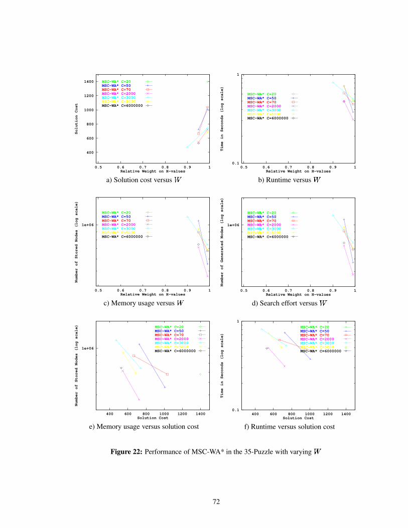
400
600
800
1000
1200
1400
0.5 0.6 0.7 0.8 0.9 1
Solution Cost
Relative Weight on H-values
MSC-WA* C=20 MSC-WA* C=50 MSC-WA* C=70 MSC-WA* C=2000 MSC-WA* C=3000 MSC-WA* C=5000 MSC-WA* C=6000000
a) Solution cost versus
0.1
1
0.5 0.6 0.7 0.8 0.9 1
Time in Seconds (log scale)
Relative Weight on H-values
MSC-WA* C=20 MSC-WA* C=50 MSC-WA* C=70 MSC-WA* C=2000 MSC-WA* C=3000 MSC-WA* C=5000 MSC-WA* C=6000000
b) Runtime versus
1e+06
0.5 0.6 0.7 0.8 0.9 1
Number of Stored Nodes (log scale)
Relative Weight on H-values
MSC-WA* C=20 MSC-WA* C=50 MSC-WA* C=70 MSC-WA* C=2000 MSC-WA* C=3000 MSC-WA* C=5000 MSC-WA* C=6000000
c) Memory usage versus
1e+06
0.5 0.6 0.7 0.8 0.9 1
Number of Generated Nodes (log scale)
Relative Weight on H-values
MSC-WA* C=20 MSC-WA* C=50 MSC-WA* C=70 MSC-WA* C=2000 MSC-WA* C=3000 MSC-WA* C=5000 MSC-WA* C=6000000
d) Search effort versus
1e+06
400 600 800 1000 1200 1400
Number of Stored Nodes (log scale)
Solution Cost
MSC-WA* C=20 MSC-WA* C=50 MSC-WA* C=70 MSC-WA* C=2000 MSC-WA* C=3000 MSC-WA* C=5000 MSC-WA* C=6000000
e) Memory usage versus solution cost
0.1
1
400 600 800 1000 1200 1400
Time in Seconds (log scale)
Solution Cost
MSC-WA* C=20 MSC-WA* C=50 MSC-WA* C=70 MSC-WA* C=2000 MSC-WA* C=3000 MSC-WA* C=5000 MSC-WA* C=6000000
f) Runtime versus solution cost
Figure 22: Performance of MSC-WA* in the 35-Puzzle with varying
72

400
600
800
1000
1200
1400
1 10 100 1000 10000 100000 1e+06
Solution Cost
Value of C (log scale)
MSC-WA* W=0.99MSC-WA* W=0.95MSC-WA* W=0.90
a) Solution cost versus �
0.1
0.2
0.3
0.4
0.5
0.6
0.7
0.8
0.9
1
1 10 100 1000 10000 100000 1e+06
Time in Seconds
Value of C (log scale)
MSC-WA* W=0.90MSC-WA* W=0.95MSC-WA* W=0.99
b) Runtime versus �
400000
600000
800000
1e+06
1.2e+06
1.4e+06
1 10 100 1000 10000 100000 1e+06
Number of Stored Nodes
Value of C (log scale)
MSC-WA* W=0.90MSC-WA* W=0.95MSC-WA* W=0.99
c) Memory usage versus �
400000
600000
800000
1e+06
1.2e+06
1.4e+06
1 10 100 1000 10000 100000 1e+06
Number of Generated Nodes
Value of C (log scale)
MSC-WA* W=0.90MSC-WA* W=0.95MSC-WA* W=0.99
d) Search effort versus �
400000
600000
800000
1e+06
1.2e+06
1.4e+06
1000
Number of Stored Nodes
Solution Cost (log scale)
MSC-WA* W=0.90MSC-WA* W=0.95MSC-WA* W=0.99
e) Memory usage versus solution cost
0.1
0.2
0.3
0.4
0.5
0.6
0.7
0.8
0.9
1
1000
Time in Seconds
Solution Cost (log scale)
MSC-WA* W=0.90MSC-WA* W=0.95MSC-WA* W=0.99
f) Runtime versus solution cost
Figure 23: Performance of MSC-WA* in the 35-Puzzle with varying �
73
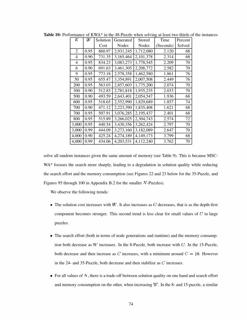
Table 10: Performance of KWA* in the 48-Puzzle when solving at least two thirds of the instances� Solution Generated Stored Time Percent
Cost Nodes Nodes (Seconds) Solved2 0.95 860.97 2,931,245 1,712,080 2.120 684 0.90 731.35 3,165,464 2,101,378 2.314 684 0.95 834.23 3,083,273 1,778,545 2.209 706 0.90 691.63 3,461,305 2,208,772 2.582 709 0.95 773.18 2,578,358 1,462,580 1.861 76
50 0.95 655.47 3,354,891 2,007,508 2.449 76200 0.95 563.03 2,857,603 1,775,200 2.074 70300 0.90 512.83 2,781,818 1,935,235 2.033 70500 0.90 493.59 2,643,401 2,054,547 1.936 68600 0.95 518.65 2,552,990 1,829,689 1.857 74700 0.90 471.12 2,223,390 1,835,408 1.621 68700 0.95 507.91 3,076,285 2,195,437 2.401 68800 0.95 515.89 3,266,025 2,304,743 2.574 72
3,000 0.95 440.54 3,430,356 3,262,424 2.797 703,000 0.99 444.09 3,273,160 3,182,089 2.647 704,000 0.90 425.24 4,274,189 4,149,173 3.799 684,000 0.99 434.06 4,203,531 4,112,240 3.762 70
solve all random instances given the same amount of memory (see Table 9). This is because MSC-
WA* focuses the search more sharply, leading to a degradation in solution quality while reducing
the search effort and the memory consumption (see Figures 22 and 23 below for the 35-Puzzle, and
Figures 95 through 100 in Appendix B.2 for the smaller�
-Puzzles).
We observe the following trends:
k The solution cost increases with . It also increases as � decreases, that is as the depth-first
component becomes stronger. This second trend is less clear for small values of � in large
puzzles.
k The search effort (both in terms of node generations and runtime) and the memory consump-
tion both decrease as increases. In the 8-Puzzle, both increase with � . In the 15-Puzzle,
both decrease and then increase as � increases, with a minimum around �O��Qm . However
in the 24- and 35-Puzzle, both decrease and then stabilize as � increases.
k For all values of�
, there is a trade-off between solution quality on one hand and search effort
and memory consumption on the other, when increasing . In the 8- and 15-puzzle, a similar
74

Table 11: Performance of MSC-WA* in the 48-Puzzle when solving at least two thirds of theinstances
� Solution Generated Stored Time PercentCost Nodes Nodes (Seconds) Solved
60 0.99 1,861.61 2,239,906 2,190,618 1.735 7290 0.99 1,763.03 2,412,524 2,353,818 1.983 72
200 0.99 1,540.26 1,998,260 1,947,644 1.526 76400 0.99 1,292.91 2,304,667 2,243,993 1.781 68900 0.99 1,273.15 2,581,034 2,507,904 2.049 78
30,000 0.95 878.29 2,256,880 2,201,531 1.747 68
trade-off exists when decreasing � (the trend is clearer for small values of and large values
of � ). In the 24- and 35-puzzle, the trend is reversed since increasing � reduces the solution
cost, the search effort, and the memory consumption (except for small values of and large
values of � ).
The results in large domains indicate that a large is crucial to reducing the memory con-
sumption. After fixing close to 1, � should probably be increased as much as possible until
memory runs out, since increasing � reduces both the solution cost and the memory consumption,
up to a certain point. Indeed, this is confirmed in the 48-Puzzle (see Table 11). The highest success
rates are achieved for high values of . Additionally, larger values of � seem to decrease the solu-
tion cost while maintaining the memory consumption approximately constant, up to a point which
unfortunately is not sufficient for MSC-WA* to solve all random instances of the 48-Puzzle.
3.6.5.4 Empirical evaluation of MSC-KWA* in the�
-Puzzle
MSC-KWA* has three parameters. These, when crossed with the different values for�
, generate
a large number of experimental conditions. So for now, we eliminate one parameter by making �equal to � . This section reports results for this special case. The general case (where � varies
between 1 and � ) is discussed in Section 3.8 .
Appendix B.3 contains all of the results of this study. We summarize them here by including
a representative sub-set of the figures pertaining to the 35-Puzzle (see Figures 24 through 28). We
observe the following trends:
k MSC-KWA* shares with WA*, KWA* and MSC-WA* the property that its search effort (that
is, the number of generated nodes), runtime (in seconds), and memory consumption (that
75
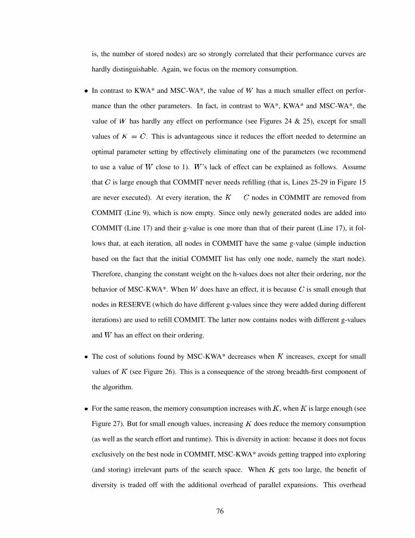
is, the number of stored nodes) are so strongly correlated that their performance curves are
hardly distinguishable. Again, we focus on the memory consumption.
k In contrast to KWA* and MSC-WA*, the value of has a much smaller effect on perfor-
mance than the other parameters. In fact, in contrast to WA*, KWA* and MSC-WA*, the
value of has hardly any effect on performance (see Figures 24 & 25), except for small
values of � � � . This is advantageous since it reduces the effort needed to determine an
optimal parameter setting by effectively eliminating one of the parameters (we recommend
to use a value of close to 1). ’s lack of effect can be explained as follows. Assume
that � is large enough that COMMIT never needs refilling (that is, Lines 25-29 in Figure 15
are never executed). At every iteration, the � � � nodes in COMMIT are removed from
COMMIT (Line 9), which is now empty. Since only newly generated nodes are added into
COMMIT (Line 17) and their g-value is one more than that of their parent (Line 17), it fol-
lows that, at each iteration, all nodes in COMMIT have the same g-value (simple induction
based on the fact that the initial COMMIT list has only one node, namely the start node).
Therefore, changing the constant weight on the h-values does not alter their ordering, nor the
behavior of MSC-KWA*. When does have an effect, it is because � is small enough that
nodes in RESERVE (which do have different g-values since they were added during different
iterations) are used to refill COMMIT. The latter now contains nodes with different g-values
and has an effect on their ordering.
k The cost of solutions found by MSC-KWA* decreases when � increases, except for small
values of � (see Figure 26). This is a consequence of the strong breadth-first component of
the algorithm.
k For the same reason, the memory consumption increases with � , when � is large enough (see
Figure 27). But for small enough values, increasing � does reduce the memory consumption
(as well as the search effort and runtime). This is diversity in action: because it does not focus
exclusively on the best node in COMMIT, MSC-KWA* avoids getting trapped into exploring
(and storing) irrelevant parts of the search space. When � gets too large, the benefit of
diversity is traded off with the additional overhead of parallel expansions. This overhead
76
100
1000
10000
0.5 0.6 0.7 0.8 0.9 1
Solution Cost (log scale)
Relative Weight on H-values
MSC-KWA* K=2 MSC-KWA* K=3 MSC-KWA* K=4 MSC-KWA* K=5 MSC-KWA* K=10 MSC-KWA* K=100 MSC-KWA* K=1000 MSC-KWA* K=7000
Figure 24: Solution cost versus for MSC-KWA* ( �/��� ) in the 35-Puzzle
100000
1e+06
0.5 0.6 0.7 0.8 0.9 1
Number of Stored Nodes (log scale)
Relative Weight on H-values
MSC-KWA* K=7000MSC-KWA* K=1000MSC-KWA* K=100 MSC-KWA* K=10 MSC-KWA* K=5 MSC-KWA* K=4 MSC-KWA* K=3 MSC-KWA* K=2
Figure 25: Memory usage versus for MSC-KWA* ( ��� � ) in the 35-Puzzle
increases with � and it cancels out the benefit of diversity for very large values of � .
k Figure 28 illustrates the trade-off exhibited by MSC-KWA* between solution cost and mem-
ory requirements: decreasing � (up to a point) sacrifices solution quality for a reduced mem-
ory consumption. The reason why each curve in the figure (except for small values of � )
reduces to a point is that the curve represents performance variations caused by varying ;
and we explained earlier why varying has little effect.
77

100
1000
10000
1 10 100 1000
Solution Cost (log scale)
Value of K (log scale)
MSC-KWA* W=0.99MSC-KWA* W=0.95MSC-KWA* W=0.90MSC-KWA* W=0.86MSC-KWA* W=0.80MSC-KWA* W=0.75MSC-KWA* W=0.67MSC-KWA* W=0.60MSC-KWA* W=0.56MSC-KWA* W=0.50
Figure 26: Solution cost versus � for MSC-KWA* ( ��� � ) in the 35-Puzzle
100000
1e+06
1 10 100 1000
Number of Stored Nodes (log scale)
Value of K (log scale)
MSC-KWA* W=0.50MSC-KWA* W=0.56MSC-KWA* W=0.60MSC-KWA* W=0.67MSC-KWA* W=0.75MSC-KWA* W=0.80MSC-KWA* W=0.86MSC-KWA* W=0.90MSC-KWA* W=0.95MSC-KWA* W=0.99
Figure 27: Memory usage versus � for MSC-KWA* ( �/��� ) in the 35-Puzzle
100000
1e+06
100 1000 10000
Number of Stored Nodes (log scale)
Solution Cost (log scale)
MSC-KWA* K=7000MSC-KWA* K=1000MSC-KWA* K=100 MSC-KWA* K=10 MSC-KWA* K=5 MSC-KWA* K=4 MSC-KWA* K=3 MSC-KWA* K=2
Figure 28: Memory usage versus solution cost for MSC-KWA* ( � � � ) in the 35-Puzzle withvarying
78

100
1000
10000
10 20 30 40 50 60 70 80 90 100
Number of Stored Nodes (log scale)
Solution Cost
WA*KWA*
MSC-WA*MSC-KWA*
a) 8-Puzzle
1000
10000
100000
1e+06
100
Number of Stored Nodes (log scale)
Solution Cost (log scale)
WA*KWA*
MSC-WA*MSC-KWA*
b) 15-Puzzle
10000
100000
1e+06
100 1000
Number of Stored Nodes (log scale)
Solution Cost (log scale)
WA*KWA*
MSC-WA*MSC-KWA*
c) 24-Puzzle
100000
1e+06
100 1000 10000
Number of Stored Nodes (log scale)
Solution Cost (log scale)
KWA*MSC-WA*MSC-KWA*
d) 35-Puzzle
1e+06
10000 100000
Number of Stored Nodes (log scale)
Solution Cost (log scale)
MSC-KWA*
c) 48-Puzzle
Figure 29: Performance comparison: WA*, KWA*, MSC-WA*, and MSC-KWA* in the�
-Puzzle
79

3.6.5.5 Empirical comparison of WA*, KWA*, MSC-WA*, and MSC-KWA* in the�
-Puzzle
In order to obtain a more synthetic view of the behavior of MSC-KWA*, we perform the same curve-
minimization process described in Section 3.5.1 to represent the performance of MSC-KWA* with
a single curve. We plot this curve against the corresponding ones for WA*, KWA*, and MSC-WA*
for different values of�
. Figure 29 shows that:
k MSC-KWA* approximates the behavior of KWA* for large values of � , yielding solutions
of high quality.
k MSC-KWA* approximates, and even significantly improves on, the behavior of MSC-WA*
for smaller values of � , yielding a low memory consumption.
k The improvement of MSC-KWA* over both KWA* and MSC-WA* in terms of memory con-
sumption grows larger when the problem gets larger. For� ��z , there is no significant
improvement over MSC-WA*. For� ��� � through Ì � , the reduction in the memory con-
sumption both increases in amplitude and starts with larger and larger values of � (that is,
more and more toward the left of the figure). Finally, MSC-KWA* is the only algorithm
among the four tested that can solve all instances of the 48-Puzzle.
To conclude, Table 12 builds on Table 8 by adding the performance of MSC-KWA*. We observe
that MSC-KWA* dominates all other algorithms in terms of memory consumption, search effort,
and runtime (when using each algorithm’s ideal settings for each performance measure) for all
tested sizes of the�
-Puzzle. Furthermore, MSC-KWA* dominates WA* and MSC-WA* in terms
of solution quality for all sizes of the�
-Puzzle. Finally, MSC-KWA* is always within about three
percent of the best algorithm (namely KWA*) in terms of solution quality.
3.6.6 Empirical results in the 4-peg Towers of Hanoi domain
We have tested the variants of WA* in the 4-peg Towers of Hanoi domain. Table 13 shows the
parameter settings (and resulting performance data) for which each algorithm solves the largest
percentage of instances (and with the smallest average solution cost) with up to one million nodes
in memory. None of the WA*, KWA*, and MSC-WA* algorithms can solve all of our fifty random
instances. Nevertheless, both MSC-WA* and KWA* scale up slightly better than WA*. Finally,
80

Table 12: Comparison of WA*, KWA*, MSC-WA*, and MSC-KWA* in the�
-Puzzle� Perf. WA* KWA* MSC-WA* MSC-KWA*
Measure Value � Best Value � � Best Value � � Best Value � � Best
8
Min Cost 21.85 0.50 � 21.85 0.50 2 � 22.01 0.50 800 � 21.85 0.99 600 �Min Sto. 452 0.86 464 0.86 2 292 0.80 2 � 290 0.95 2 �Min Gen. 514 0.86 519 0.99 4 296 0.80 2 � 294 0.95 2 �Min Time
15
Min Cost 63.51 0.67 53.85 0.67 50K � 56.29 0.60 80K 53.89 0.99 50K �Min Sto. 6,050 0.99 6,028 0.99 8 4,113 0.95 20 3,223 0.99 5 �Min Gen. 6,972 0.99 6,704 0.99 8 4,191 0.95 20 3,259 0.99 5 �Min Time 0.003 0.99 0.003 0.99 5 0.002 0.99 6 0.001 0.95 3 �
24
Min Cost 165.16 0.75 113.56 0.99 20K � 164.56 0.75 90K 116.32 0.99 20KMin Sto. 44,097 0.99 32,567 0.99 5 36,907 0.99 300 16,178 0.99 6 �Min Gen. 56,070 0.99 43,578 0.99 4 37,832 0.99 300 16,331 0.99 6 �Min Time 0.027 0.99 0.021 0.99 4 0.021 0.99 50K 0.007 0.99 6 �
35
Min Cost 236.50 0.99 7K � 472.10 0.90 3K 244.14 0.99 7KMin Sto. 417,675 0.95 20 456,777 0.99 90 56,807 0.99 5 �Min Gen. 652,100 0.95 500 467,586 0.99 90 57,291 0.99 5 �Min Time 0.377 0.95 500 0.297 0.99 90 0.033 0.99 5 �
48
Min Cost 18,379.32 0.60 5 �Min Sto. 275,293 0.80 4 �Min Gen. 277,282 0.80 4 �Min Time 0.181 0.80 4 �
Table 13: Best performance of all algorithms in the Towers of Hanoi domain (memory = 1 millionnodes)
Algorithm � � Solution Generated Stored Time PercentCost Nodes Nodes (Seconds) Solved
WA* q 1 0.99 629.88 2,323,424 762,638 1.582 84KWA* N/A 3 0.99 629.68 2,278,109 749,782 1.551 88MSC-WA* 600 N/A 0.99 672.66 2,059,218 750,125 1.587 94MSC-KWA* 100 100 1.00 3,762.33 1,431,303 675,450 0.976 72MSC-KWA* 40,000 177 1.00 2,261.76 1,664,383 750,326 1.139 100
81

Table 14: Performance of MSC-KWA* in the Towers of Hanoi domain when solving all instances(memory = 1 million nodes)
� � Solution Generated Stored Time PercentCost Nodes Nodes (Seconds) Solved
20,000 93 1.00 3,877.66 1,516,603 727,983 1.058 10020,000 117 1.00 2,949.94 1,540,506 709,424 1.095 10020,000 120 1.00 2,922.56 1,664,459 755,601 1.193 10030,000 75 1.00 4,261.12 1,529,075 723,398 1.120 10030,000 96 1.00 3,492.08 1,450,032 688,717 0.991 10030,000 111 1.00 3,387.04 1,671,093 766,913 1.167 10030,000 129 1.00 2,576.00 1,506,882 693,956 1.056 10040,000 132 1.00 2,866.26 1,621,793 748,193 1.117 10040,000 177 1.00 2,261.76 1,664,383 750,326 1.139 10050,000 111 1.00 3,406.30 1,639,262 763,766 1.254 10050,000 135 1.00 2,742.02 1,619,731 744,240 1.212 100
MSC-KWA* is the only one of our contenders that can solve all of our random instances within the
same memory bound. The next-to-last line in the table reports the best performance of MSC-KWA*
when �/��� .
Table 14 shows parameter settings (and the resulting performance data) for which MSC-KWA*
is complete over our full set of random instances. We observe the following trends. First, the relative
weight on the h-values is always maximum (namely equal to 1). Second, the level of commitment
is relatively low (i.e., � is relatively large, on the order of a few tens of thousands) but still higher
than that of WA* (for which � ��q ). Third, the level of diversity is relatively small (in particular,
��nC� ) but still two orders of magnitude larger than for WA* (namely, � is on the order of 100
versus 1 for WA*). In conclusion, in our empirical setup for this domain, MSC-KWA* scales up to
larger (namely, 22-disk) problems than any of the other tested algorithms. Therefore, the right mix
of commitment and diversity boosts the performance of WA* significantly in this domain.
3.6.7 Empirical results in the Rubik’s Cube domain
Table 15 shows the parameter settings (and resulting performance data) for which each algorithm
solves the largest percentage of instances in the Rubik’s Cube domain with up to two million nodes
in memory. No algorithm solves all instances. However, each variant of WA* improves upon
it. MSC-KWA* solves more instances than MSC-WA*, which in turn solves more instances than
KWA*. Note that the best scaling behavior of MSC-KWA* is obtained for different values of �
82
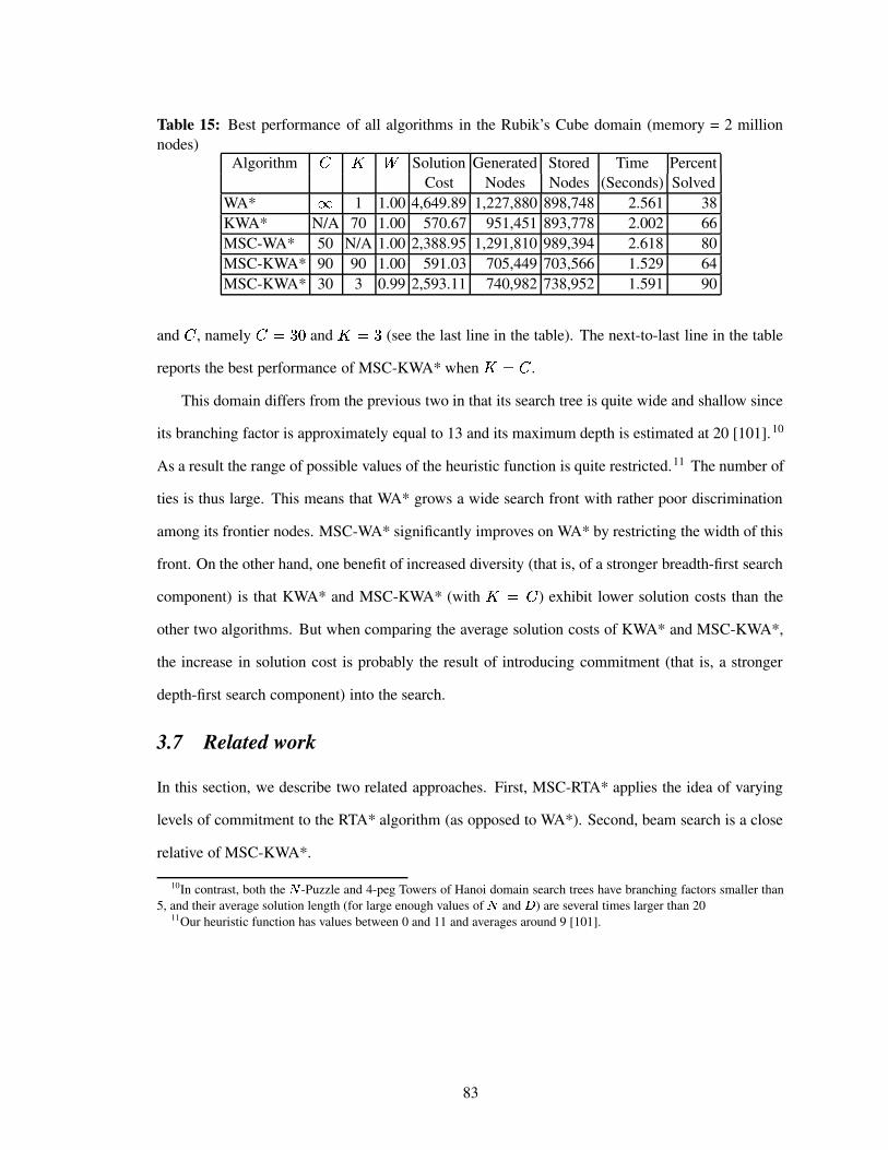
Table 15: Best performance of all algorithms in the Rubik’s Cube domain (memory = 2 millionnodes)
Algorithm � � Solution Generated Stored Time PercentCost Nodes Nodes (Seconds) Solved
WA* q 1 1.00 4,649.89 1,227,880 898,748 2.561 38KWA* N/A 70 1.00 570.67 951,451 893,778 2.002 66MSC-WA* 50 N/A 1.00 2,388.95 1,291,810 989,394 2.618 80MSC-KWA* 90 90 1.00 591.03 705,449 703,566 1.529 64MSC-KWA* 30 3 0.99 2,593.11 740,982 738,952 1.591 90
and � , namely �F� ÌYm and � � Ì (see the last line in the table). The next-to-last line in the table
reports the best performance of MSC-KWA* when ��� � .
This domain differs from the previous two in that its search tree is quite wide and shallow since
its branching factor is approximately equal to 13 and its maximum depth is estimated at 20 [101].10
As a result the range of possible values of the heuristic function is quite restricted.11 The number of
ties is thus large. This means that WA* grows a wide search front with rather poor discrimination
among its frontier nodes. MSC-WA* significantly improves on WA* by restricting the width of this
front. On the other hand, one benefit of increased diversity (that is, of a stronger breadth-first search
component) is that KWA* and MSC-KWA* (with � �/� ) exhibit lower solution costs than the
other two algorithms. But when comparing the average solution costs of KWA* and MSC-KWA*,
the increase in solution cost is probably the result of introducing commitment (that is, a stronger
depth-first search component) into the search.
3.7 Related work
In this section, we describe two related approaches. First, MSC-RTA* applies the idea of varying
levels of commitment to the RTA* algorithm (as opposed to WA*). Second, beam search is a close
relative of MSC-KWA*.
10In contrast, both the � -Puzzle and 4-peg Towers of Hanoi domain search trees have branching factors smaller than5, and their average solution length (for large enough values of � and � ) are several times larger than 20
11Our heuristic function has values between 0 and 11 and averages around 9 [101].
83

1. procedure RTA*( :�36587�9:5 , ;=<?>A@CBED"F6B:G�%¨P�, ): solution cost2. � %�: 3�587�9:5 , := m ; � %�: 3�587�9:5 , := ;A<?>A@"B|D?F6B6Ga%�: 3�587�9:5 ,3. D"Fa`TFb< := :H36587�9:54. ��<"D?F|� := q ; D�< G� T¡d¢�£¤<"D?F|� := q ; ��<"D?F�W := ¥5. for each successor : of D"Fa`TFb< do6. if ( :À�":<xcy ucz ) then return � %�D?Fa`TFb<{, � �7. if ( : is newly generated ) then8. � %�:Y, := � %�D?Fa`TFb<@, � � ; � %�:Y, := ;A<J>A@CBED"F6B:Ga%�:Y,9. if ( � %�:�,¶�¦�C<"D?F|� ) then DJ<�G� +¡d¢&£§<?D"F|� := �C<"D"F|� ; ��<"D?F|� := � %�:Y, ; �C<"D"F�W := :
10. else if ( � %�:Y,¾n_DJ<�G� +¡ ¢�£¤<"D"F|� ) then DJ< GC +¡d¢�£¤<?D"F|� := � %�:Y,11. end for12. � %�D"Fa`TFb<�, := max( � %�D?Fa`TFb<{, , � � DJ<�G� +¡ ¢�£¤<"D"F|� )13. if ( �C<"D?F�W��¨¥ ) then return q14. else D"Fa`TFb< := ��<"D?F�W15. go to Line 4
Figure 30: The RTA* algorithm
3.7.1 Multi-state commitment applied to RTA* search
In [88], the idea of multi-state commitment is applied, not only to WA*, but also to RTA* [98]. In
this section, we describe the RTA* and resulting MSC-RTA* algorithms.
3.7.1.1 The RTA* algorithm
The RTA* algorithm is a variant of the LRTA* algorithm [98]. The only difference between LRTA*
and RTA* is the way they update the h-value of the current state. While LRTA* sets it to the
estimated cost of a shortest path from the state to a goal, RTA* sets it to the second best estimate.
The motivation for RTA* is that, since the algorithm always moves to a successor that minimizes the
estimated cost to a goal, re-visiting the state is only worth it if one of its other successor becomes
the most promising (since the best one was just visited). There are two important consequences of
this change in the value-update rule. First, RTA* typically finds shorter solutions that LRTA* [98].
Second, even if the initial h-values are admissible, the updated ones may not be. Therefore, RTA*
(unlike LRTA*) is not guaranteed to converge to an optimal path after repeated trials. In this work
(like in [88]), we use RTA* as an approximation algorithm to the shortest-path problem, not as a
real-time search algorithm (that is, one that interleaves planning and plan execution). We are only
interested in the first trial of RTA*, namely until it reaches a goal state for the first time.
84

Figure 30 contains the pseudo-code for RTA*. As always in this chapter, 1) we assume that
there is a single goal, 2) we assume that all actions have unit cost, and 3) we omit the description of
the mechanism (that is, the management of back-pointers) used to reconstruct the solution found.
3.7.1.2 The MSC-RTA* algorithm
[88] points out that WA* and RTA* are the two extremes of a spectrum characterized by the notion
of commitment. WA* does not make any commitment since any open node can be expanded next.
In contrast, RTA* is maximally committed since the next node to be expanded is always selected
among the successors of a single node, namely the latest node expanded. Multi-state commitment
search is a middle ground between RTA* and WA*, since the set of candidate nodes for expansions
is kept constant between one and the size of the OPEN list. [88] describes two approaches for
multi-state commitment search. First, adding commitment to WA* results in MSC-WA*. Second,
decreasing commitment in RTA* results in MSC-RTA*, which we focus on in this section.
Figure 31 contains the pseudo-code for MSC-RTA*. Like MSC-WA*, MSC-RTA* maintains a
COMMIT list (of fixed maximum size � ) among which it chooses the next node to expand. Nodes
in COMMIT are ordered according to increasing h-values. The list is initialized with the start state
(Line 2). During each iteration (Lines 3-32), the best state is selected as the current state (Line 4)
and removed from COMMIT (Line 5), and its successors are added into COMMIT (Lines 6-26).
Then, the h-value of the current state is updated, like in RTA* (Line 27). Finally, the worst nodes in
COMMIT are pruned if necessary to keep its size no greater than � (Lines 28-31). The algorithm
terminates when the goal state is generated for the first time (Line 8) or when COMMIT becomes
empty (Line 3).
In our version of MSC-RTA* (these details are not provided in [88]), a successor is only added
into COMMIT if either the list is not full (Lines 11&19) or the h-value of the successor is less
than that of the worst node in COMMIT (Lines 13&21), in which case this worst node is replaced
with the successor (Lines 14-15 & 22-23). Only nodes that have been in COMMIT are stored in
memory. The other generated successors are not stored. Whereas RTA* only stores the successor of
the current state it moves to, MSC-RTA* stores a percentage (between 0 and 100 percent included)
of the successors of the current state, depending on the distribution of their h-values and those of
85

1. procedure MSC-RTA*( :4365I7 9:5 , ;A<?>A@"B|D?F6B6Ga%¨P�, , � ): solution cost2. � %�:H3�587�9:5¨, := m ; � %�:H3�587�9:5¨, := ;A<?>A@"B|D?F6B6Ga%�:H3�587�9:5¨, ; L*MONPNRQTS := M�:H36587�9:54T3. while ( L*MONPNPQTS���_[ ) do4. D?Fa`TFb< := arg min r4£dceKf*fqg hJM � %�:Y,2T5. L*MONRNPQTS := L*MONPNPQTS�j�MTD"Fa`TFb<�T6. �C<"D"F|� := q ; DJ<�G� +¡d¢&£§<?D"F|� := q7. for each successor : of D?Fa`TFb< do8. if ( :À��:�xcy ucz ) then return � %�D"Fa`TFb<�, � �9. if ( : is newly generated ) then
10. � %�:Y, := � %�D"Fa`TFb<@, � � ; � %�:�, := ;A<?>A@"B|D?F6B6G�%�:Y,11. if ( s6L*MONRNPQTS�san�� ) then L*MONRNPQTS := L*MONPNPQTSrk�M�:@T12. else ©O +@CD"F := arg max r+£�c�eKfXfXg h M � %�:Y,2T13. if ( � %�:�,^n � %/©O +@CD"Ff, ) then14. L*MONPNRQTS := L*MONRNPQTS�j�MH©O +@CD"FQT15. L*MONPNRQTS := L*MONRNPQTS�k�M�:{T16. else17. � %�:Y, := min( � %�:�,b( � %�D"Fa`TFb<a, � � )18. if ( :8�7oL*MONPNRQTS ) then19. if ( s6L*MONRNPQTS�s�n9� ) then L*MONRNPQTS := L*MONPNRQTS�k�M�:{T20. else ©O +@CD"F := arg max r+£�c�eKfXfXg hJM � %�:Y,2T21. if ( � %�:�,^n � %/©O +@CD"Ff, ) then22. L*MONPNRQTS := L*MONRNPQTS�j�MH©O T@�D?F?T23. L*MONPNRQTS := L*MONRNPQTS�k�M�:@T24. if ( � %�:Y,¾�¦�C<"D"F|� ) then D�< GC +¡d¢�£¤<"D?F|� := ��<?D"F|� ; ��<?D"F|� := � %�:Y,25. else if ( � %�:�,¾n¨DJ< GC +¡d¢�£¤<?D"F|� ) then D�< G� T¡d¢�£¤<"D?F|� := � %�:Y,26. end for27. � %�D?Fa`TFb<{, := max( � %�D"Fa`HFb<@, , � � DJ< GC +¡d¢�£¤<?D"F|� )28. while ( s6L*MONPNRQTS�s�|9� ) do29. D"Fa`TFb< := arg max r+£�ceKf*fXg�h�M � %�:�,GT30. L*MONPNPQTS := L*MONPNRQTS�j�MTD"Fa`HFb<�T31. end while32. end while33. return q
Figure 31: The MSC-RTA* algorithm
86

nodes currently in COMMIT. In contrast, WA* stores all generated nodes (in OPEN or CLOSED).
This is another dimension along which MSC-RTA* lies between RTA* and WA*.
When ��� � , MSC-RTA* starts and ends each iteration (except the last one) with only one
node in COMMIT. During the iteration, the current state is removed from COMMIT and succes-
sively replaced with (a sub-set of) its successors in decreasing order of their h-values until the best
successor remains in COMMIT at the end of the iteration. Since this node is selected as current
node at the beginning of the next iteration, MSC-RTA* with �}��� is functionally equivalent to
RTA* (but with the additional overhead of maintaining the COMMIT list).
When � ��q , the COMMIT list never fills up. All generated nodes are thus added into
COMMIT (and stored in memory). In this case, MSC-RTA* grows a full search frontier, like WA*.
The main differences are that MSC-RTA* can re-expands some nodes and that it updates the h-value
of the expanded node.
MSC-RTA* is to RTA* as MSC-WA* is to WA*: both multi-state commitment search algo-
rithms vary the level of commitment of the basic algorithm they modify. Furthermore, MSC-RTA*,
like MSC-WA*, only expands one node at each iteration. Studying the effect of introducing diver-
sity into MSC-RTA is an interesting direction for future research (see Section 3.8.3).
3.7.2 Beam search
Beam search is another algorithm that takes advantage of a strong commitment to scale up heuristic
search to larger problems [7, 170]. Beam search is typically a variant of best-first search in which
only a fixed number (called the width of the beam) of nodes are considered for expansion at each
iteration. The beam width is thus equivalent to the size of the commitment list in MSC-WA* and
MSC-KWA*.
Furthermore, beam search typically expands all the nodes under consideration in parallel [7,
170]. In other words, beam search uses a full measure of diversity similarly to MSC-KWA* with
��� � .
Therefore, one contribution of this work is the observation that beam search can be construed
as the combination of two distinct principles (namely commitment and diversity) applied to best-
first search. In contrast, the standard view of beam search considers its strong commitment as the
87

only factor in its improved scaling behavior. Our research suggests otherwise, with diversity (that
is, parallel expansion) as another contributing factor, as demonstrated by our experiments in the�
-Puzzle, the Rubik’s Cube, and to a smaller degree in the 4-peg Towers of Hanoi domain. The
isolation of these two separate factors raises the following questions:
k What are the relative contributions of these two factors, and how do they vary across domains
and with different values of � ?
k Are there any benefits to using different levels of commitment and diversity (namely different
values for � and � )? (see Section 3.8.2 for preliminary results in the�
-puzzle)
Finally, one important difference between beam search and MSC-KWA* is that, while MSC-
KWA* keeps all discarded nodes in memory (in the RESERVE list), beam search never stores them
at all. So when the beam becomes empty, beam search has no reserved nodes available to refill it
and it must stop. On the other hand, when the beam is wide enough that it never empties out, beam
search wastes no memory on the RESERVE list. There is thus a continuum of algorithms between
beam search and MSC-KWA*. They are characterized by the size ª of the RESERVE list. As ªincreases from 0 (beam search) to infinity (MSC-KWA*), the risk of terminating without a goal
because of an empty beam decreases, whereas the risk of running out of memory before a goal is
found increases. The trade-off between these risks depends on both the structure of the search graph
(e.g., its average branching factor) and the value of � (or beam width). The empirical evaluation of
these variants of beam search, as well as their comparison against the variants of WA* discussed in
this chapter, constitute another interesting avenue of research.
3.8 Future work
In this section, we discuss possible directions for future work and present preliminary results when
available.
3.8.1 Domain-dependent behaviors of MSC-KWA*
The relative performance of heuristic search algorithms typically varies from domain to domain.
This and previous research have shown that domain-dependent effects on the relative performance
88

of our variants of WA* do exist. [88] suggests that MSC-WA* may not significantly improve on
WA* in the gridworld domain. Our research shows that the clear improvements exhibited by MSC-
KWA* over WA* and its other variants in the�
-Puzzle and Towers of Hanoi domains do not
carry over to the Rubik’s Cube domain. Further work remains to be done to understand which
characteristics of the domain (e.g., its average branching factor, the depth of the shallowest goal,
the distribution of goal states in the search tree, etc.) or the heuristic function (e.g., how well it
discriminates among states, how many ties it creates when ordering nodes for expansion, etc.) can
predict the performance of these variants of WA*. Our empirical study only uses one heuristic
function per domain. It would be interesting to study, within each domain, the effects of varying the
level of informedness of the heuristic function on the relative performance of these algorithms.
3.8.2 MSC-KWA* versus beam search
As noted earlier, MSC-KWA* is a close relative of beam search [7, 170], since they only differ in
whether to use some of the available memory for a reserve list of nodes. [47] presents the results of
our empirical comparison of beam search and MSC-KWA* in the same three domains used in this
study. Further work is also needed to study the continuum of methods identified earlier between
these two search algorithms when varying the size of the reserve list (see Section 3.7.2).
Furthermore, our description of both MSC-KWA* and beam search as committed and diver-
sified variants of best-first search suggests the possibility of teasing out the effects of these two
distinct principles on the overall behavior. In particular, we have so far only considered the situation
where the levels of commitment and diversity are equal, which is the case both in MSC-KWA* with
� = � and in beam search. But could different levels of diversity and commitment lead to better
performance? We briefly address this issue for MSC-KWA* in the following sub-section.
3.8.2.1 Preliminary study of MSC-KWA* with �E�� �9� in the�
-Puzzle
Since MSC-KWA* makes it possible to fine-tune the relative contributions of commitment (through
� ) and diversity (through � ), we vary both � and � (in addition to ) and run MSC-KWA* in
the 48-Puzzle. Our goal is to determine empirically whether some combinations of distinct values
for � and � improve the behavior of MSC-KWA*.
89
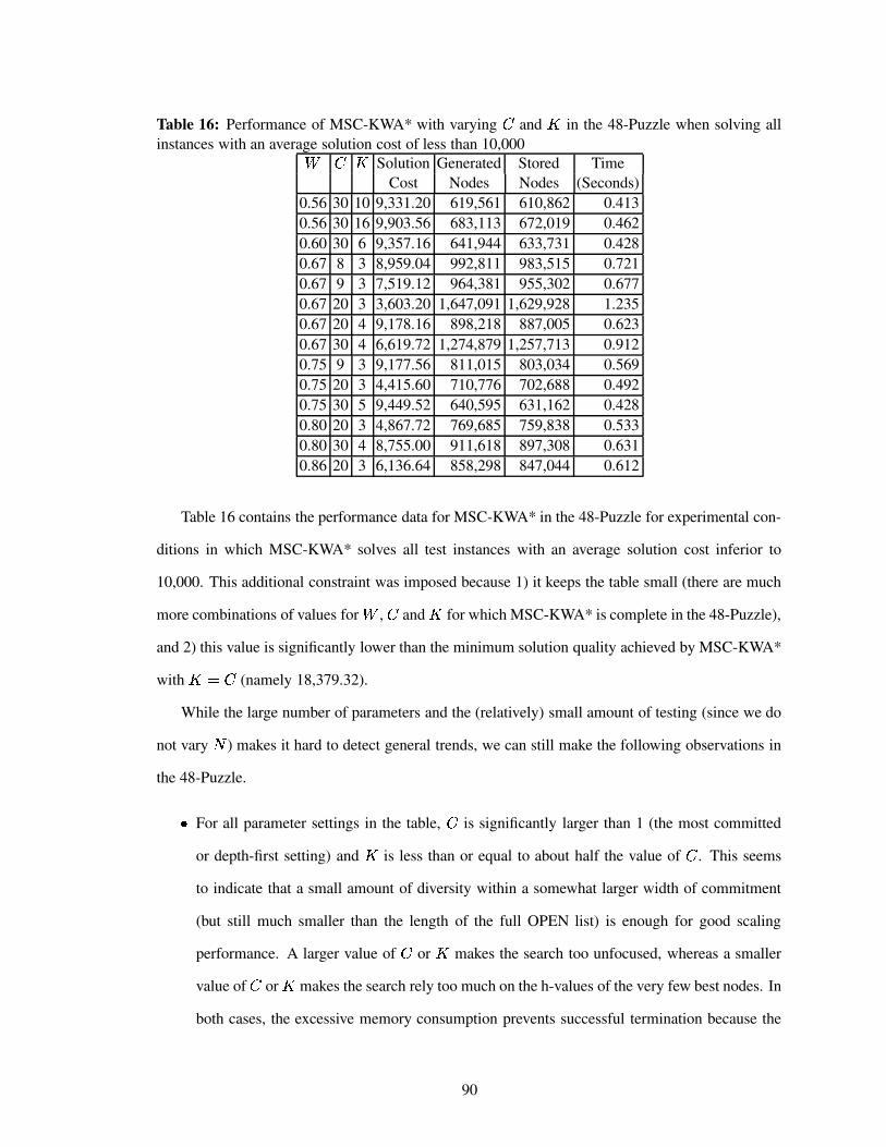
Table 16: Performance of MSC-KWA* with varying � and � in the 48-Puzzle when solving allinstances with an average solution cost of less than 10,000
� � Solution Generated Stored TimeCost Nodes Nodes (Seconds)
0.56 30 10 9,331.20 619,561 610,862 0.4130.56 30 16 9,903.56 683,113 672,019 0.4620.60 30 6 9,357.16 641,944 633,731 0.4280.67 8 3 8,959.04 992,811 983,515 0.7210.67 9 3 7,519.12 964,381 955,302 0.6770.67 20 3 3,603.20 1,647,091 1,629,928 1.2350.67 20 4 9,178.16 898,218 887,005 0.6230.67 30 4 6,619.72 1,274,879 1,257,713 0.9120.75 9 3 9,177.56 811,015 803,034 0.5690.75 20 3 4,415.60 710,776 702,688 0.4920.75 30 5 9,449.52 640,595 631,162 0.4280.80 20 3 4,867.72 769,685 759,838 0.5330.80 30 4 8,755.00 911,618 897,308 0.6310.86 20 3 6,136.64 858,298 847,044 0.612
Table 16 contains the performance data for MSC-KWA* in the 48-Puzzle for experimental con-
ditions in which MSC-KWA* solves all test instances with an average solution cost inferior to
10,000. This additional constraint was imposed because 1) it keeps the table small (there are much
more combinations of values for , � and � for which MSC-KWA* is complete in the 48-Puzzle),
and 2) this value is significantly lower than the minimum solution quality achieved by MSC-KWA*
with ��� � (namely 18,379.32).
While the large number of parameters and the (relatively) small amount of testing (since we do
not vary�
) makes it hard to detect general trends, we can still make the following observations in
the 48-Puzzle.
k For all parameter settings in the table, � is significantly larger than 1 (the most committed
or depth-first setting) and � is less than or equal to about half the value of � . This seems
to indicate that a small amount of diversity within a somewhat larger width of commitment
(but still much smaller than the length of the full OPEN list) is enough for good scaling
performance. A larger value of � or � makes the search too unfocused, whereas a smaller
value of � or � makes the search rely too much on the h-values of the very few best nodes. In
both cases, the excessive memory consumption prevents successful termination because the
90
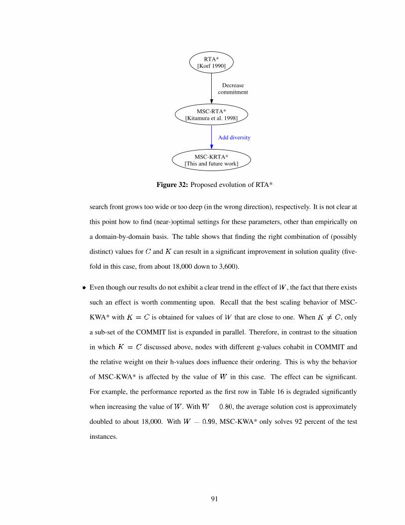
RTA*[Korf 1990]
MSC-RTA*[Kitamura et al. 1998]
Decreasecommitment
MSC-KRTA*[This and future work]
Add diversity
Figure 32: Proposed evolution of RTA*
search front grows too wide or too deep (in the wrong direction), respectively. It is not clear at
this point how to find (near-)optimal settings for these parameters, other than empirically on
a domain-by-domain basis. The table shows that finding the right combination of (possibly
distinct) values for � and � can result in a significant improvement in solution quality (five-
fold in this case, from about 18,000 down to 3,600).
k Even though our results do not exhibit a clear trend in the effect of , the fact that there exists
such an effect is worth commenting upon. Recall that the best scaling behavior of MSC-
KWA* with � ��� is obtained for values of that are close to one. When ������ , only
a sub-set of the COMMIT list is expanded in parallel. Therefore, in contrast to the situation
in which ��� � discussed above, nodes with different g-values cohabit in COMMIT and
the relative weight on their h-values does influence their ordering. This is why the behavior
of MSC-KWA* is affected by the value of in this case. The effect can be significant.
For example, the performance reported as the first row in Table 16 is degraded significantly
when increasing the value of . With ���m�P}zYm , the average solution cost is approximately
doubled to about 18,000. With � m�P}�T� , MSC-KWA* only solves 92 percent of the test
instances.
91
3.8.3 Introducing diversity in MSC-RTA*
Section 3.7.1 describes how [88] varies the level of commitment in RTA*, thus transforming the
real-time search algorithm into a best-first search algorithm called Multi-State Commitment RTA*
(MSC-RTA*). Our research naturally suggests a direction for future work, namely to study the
effects of introducing diversity into MSC-RTA*. MSC-KRTA*, the resulting algorithm, is to MSC-
RTA* as MSC-KWA* is to MSC-WA*. The proposed evolution of RTA* into MSC-KRTA* is
depicted in Figure 32. In the next sub-section, we describe MSC-KRTA* and report on a preliminary
empirical evaluation.
3.8.3.1 The MSC-KRTA* algorithm
MSC-RTA* is less committed than RTA*: as � increases, its depth-first component weakens and its
best-first component strengthens. Like WA* and RTA*, MSC-RTA* can temporarily and wastefully
get trapped in goal-free regions of the search space due to misleading h-values. To address this
problem, we propose to add diversity in the MSC-RTA* search by expanding several nodes in
parallel at each iteration.
Figure 33 contains the pseudo-code for MSC-KRTA*. The only change from MSC-RTA* are
Lines 4-9 where � nodes in COMMIT are selected for parallel expansion (in Lines 1-33). When
����� , MSC-RTA* reduces to MSC-RTA*. When ��� � , all nodes in COMMIT are expanded in
parallel.
MSC-KRTA* adds one parameter (namely � ) to the only parameter (namely � ) of MSC-RTA*.
As with MSC-KWA*, we eliminate one parameter by making � equal to � and we run MSC-RTA*
and MSC-KRTA* in the�
-Puzzle. Figure 34 compares the performance of all algorithms.
Overall, both MSC-RTA* and MSC-KRTA* seem to perform at least as well as MSC-KWA*.
In fact, as the domain gets larger, they both seem to improve on MSC-KWA* in terms of memory
consumption for large values of � . So much so that both algorithms exhibit a significantly better
memory-solution quality trade-off in the 48-Puzzle. Since one important difference between MSC-
KWA* and MSC-KRTA* is that the latter revisits nodes and can learn better informed h-values for
them, these preliminary results suggest as an interesting direction for future work the study of how
92

1. procedure MSC-KRTA*( :436587�9:5 , ;A<J>K@"BED"F6B:G�%¨P�, , � , ���o� �9� ): solution cost2. � %�:H3�587�9:5¨, := m ; � %�:H3�587�9:5¨, := ;A<?>A@"B|D?F6B6Ga%�:H3�587�9:5¨, ; L*MONPNRQTS := M�:H36587�9:54T3. while ( L*MONPNPQTS���_[ ) do4. WAV1S := [5. while ( ( L*MONPNRQTS���_[ ) and ( s}WAV1S1sanÐ� ) ) do6. D"Fa`TFb< := arg min r+£�ceKf*fXg�h M � %�:�,GT7. WAV�S := WAV1Smk�MTD?Fa`TFb<�T8. L*MONPNRQTS := L*MONRNPQTS�j�MTD?Fa`TFb<�T9. end while
10. for each D"Fa`TFb< in WAV1S do11. ��<"D?F|� := q ; D�< GC +¡d¢�£¤<"D?F|� := q12. for each successor : of D"Fa`HFb< do13. if ( :ª�":<xby ubz ) then return � %�D?Fa`TFb<{, � �14. if ( : is newly generated ) then15. � %�:Y, := � %�D?Fa`TFb<@, � � ; � %�:Y, := ;=<?>A@CBED"F6B:G�%�:�,16. if ( s6L*MONPNRQTS�s�n9� ) then L*MONPNRQTS := L*MONRNPQTSmk�M�:{T17. else ©O T@�D?F := arg max r+£�ceKf*fXg�h�M � %�:�,GT18. if ( � %�:Y,¾n � %/©O +@CD"Fb, ) then19. L*MONPNPQTS := L*MONPNRQTS�j�MH©O +@CD"F?T20. L*MONPNPQTS := L*MONPNRQTS�k�M�:{T21. else22. � %�:Y, := min( � %�:Y,b( � %�D?Fa`TFb<�, � � )23. if ( :8�7�L*MONPNRQTS ) then24. if ( s6L*MONPNRQTS�s�n9� ) then L*MONRNPQTS := L*MONRNPQTS�k�M�:@T25. else ©O T@�D?F := arg max r+£�ceKf*fXg�h�M � %�:�,6T26. if ( � %�:�,¾n � %/©O +@CD"Fb, ) then27. L*MONPNPQTS := L*MONPNRQTS�j�MH©O +@CD"F?T28. L*MONPNPQTS := L*MONPNRQTS�k�M�:{T29. if ( � %�:�,^�¦��<?D"F|� ) then DJ<�G� +¡ ¢�£¤<"D"F|� := �C<"D?F|� ; ��<"D?F|� := � %�:Y,30. else if ( � %�:Y,¾n_D�< G� T¡d¢�£¤<"D?F|� ) then DJ<�G� +¡d¢&£§<?D"F|� := � %�:�,31. end for32. � %�D"Fa`HFb<{, := max( � %�D"Fa`TFb<@, , � � D�< G� T¡d¢�£¤<"D?F|� )33. end for34. while ( s6L*MONPNRQTS�s�|9� ) do35. D"Fa`TFb< := arg max r+£�ceKf*fXg�h�M � %�:�,GT36. L*MONPNPQTS := L*MONPNRQTS�j�MTD"Fa`HFb<�T37. end while38. end while39. return q
Figure 33: The MSC-KRTA* algorithm
93

100
1000
10000
20 40 60 80 100 120
Number of Stored Nodes (log scale)
Solution Cost
WA*KWA*
MSC-WA*MSC-KWA*MSC-RTA*MSC-KRTA*
a) 8-Puzzle
1000
10000
100000
1e+06
100
Number of Stored Nodes (log scale)
Solution Cost (log scale)
WA*KWA*
MSC-WA*MSC-KWA*MSC-RTA*MSC-KRTA*
b) 15-Puzzle
10000
100000
1e+06
100 1000 10000
Number of Stored Nodes (log scale)
Solution Cost (log scale)
WA*KWA*
MSC-WA*MSC-KWA*MSC-RTA*MSC-KRTA*
c) 24-Puzzle
100000
1e+06
100 1000 10000 100000
Number of Stored Nodes (log scale)
Solution Cost (log scale)
KWA*MSC-WA*MSC-KWA*MSC-RTA*MSC-KRTA*
d) 35-Puzzle
100000
1e+06
10000 100000
Number of Stored Nodes (log scale)
Solution Cost (log scale)
MSC-KWA*MSC-RTA*MSC-KRTA*
e) 48-Puzzle
Figure 34: Performance comparison: WA*, KWA*, MSC-WA*, MSC-KWA*, MSC-RTA*, andMSC-KRTA* in the
�-Puzzle
94

100000
1e+06
10000 100000
Number of Stored Nodes (log scale)
Solution Cost (log scale)
MSC-KWA* (K=C)MSC-KWA* (K<C)MSC-RTA* MSC-KRTA* (K=C)MSC-KRTA* (K<C)
Figure 35: Performance comparison: MSC-KWA*, MSC-RTA*, and MSC-KRTA* in the 48-Puzzle
and when this learning mechanism improves performance when combined with diversity and multi-
state commitment in best-first search. Furthermore, the fact that MSC-KRTA* performs better than
MSC-RTA* in large instances of this domain provides additional support for our claim that diversity
and commitment can be combined with beneficial effects.
Finally, as is the case with MSC-KWA* (Section 3.8.2.1), a potential advantage of MSC-KRTA*
is the possibility of using different levels of commitment and diversity by setting � to a strictly
smaller value than � . Preliminary results in the 48-Puzzle reported in Figure 35 suggest that doing
so may improve the scaling behavior of MSC-KRTA*. Though the effect seems smaller than for
MSC-KWA*, further empirical evaluation remains to be done.
3.9 Conclusions
The research described in this chapter makes the following contributions.
k It provides stronger empirical support for the improved scaling behavior of MSC-WA* over
WA* by 1) measuring its search effort, solution quality and memory consumption while vary-
ing both the size of the commitment list and the relative weight on the h-values (the original
study kept this weight fixed), and by 2) testing it in two additional domains.
k It provides stronger empirical support for both the speedup and reduced memory consumption
95

(for a given solution cost) of KWA* over WA* by 1) using a slightly improved implementation
of KWA* that does scale it up to the 35-Puzzle (the original implementation did not) and 2)
by testing it in two additional domains.
k It provides the first comparison between two existing algorithms that were developed inde-
pendently. Our empirical comparison highlights the different ways in which they improve on
WA*. In the�
-Puzzle for example, we show that 1) KWA* takes advantage of its stronger
breadth-first search component to improve the solution quality, but that 2) MSC-WA* takes
advantage of its stronger depth-first search component to reduce memory consumption.
k It shows how to combine the orthogonal ideas of commitment and diversity into a new al-
gorithm called MSC-KWA* that, in two of our benchmark domains, scales up to even larger
problems than either KWA* or MSC-WA* taken individually.
k It underscores the strong similarity between MSC-KWA* and beam search. This observation
in turn provides a new view of beam search as the result of applying both commitment and
diversity to best-first search.
96

CHAPTER IV
LIMITED DISCREPANCY BEAM SEARCH �
4.1 Introduction
In Chapter 3, we applied the ideas of commitment and diversity to the WA* algorithm, resulting
in the MSC-KWA* algorithm and we showed that 1) MSC-KWA* scales up better than existing
variants of WA* and 2) MSC-KWA* is functionally similar to beam search. In fact, these two
features of MSC-KWA* and beam search are essential to scaling: commitment involves explicit
control over the width of the search tree in order to eliminate its exponential growth; and diversity
(i.e., the expansion of each full level in parallel) reduces the risk of being led astray by the heuristic
function. These observations motivate our interest in beam search.
Beam search is a well-known solution to the problem of the exponential memory requirements
of best-first search. Beam search sacrifices solution quality for reduced memory consumption by
pruning nodes that are ranked worse than the best nodes currently under consideration. , called
the bandwidth or simply the width of the beam,1 is a constant parameter that is set at the beginning of
the search. The smaller , that is the more pruning occurs at each step of the search, the less memory
beam search consumes at each level of the search tree and the larger the problem instances beam
search is able to solve. Unfortunately, more pruning typically increases the probability of discarding
good nodes and thus often reduces the solution quality. Excessive pruning can even render the search
incomplete. Therefore, the choice of a good value (or equivalently an appropriate pruning power)
depends on the amount of available memory, the optimal path cost (or alternatively the minimum
depth of the goal in the search tree) and the quality of the heuristic function (which ranks the nodes
before pruning occurs).
In this chapter, we review several existing beam search algorithms but we focus on its standard
�This chapter first appeared as [47].
1Depending on the context, beam denotes either the complete set of stored nodes at all levels of the search tree (inmost of this chapter), or only the subset of stored nodes at a given level of the search tree (in the pseudo-code of beamsearch variants and its discussion in the main text).
97
application to breadth-first search. Breadth-first-based beam search only keeps nodes at each
level of the search tree which is built in a breadth-first manner. Therefore, the memory consumption
of beam search is proportional to times the maximum search depth. Now, the available memory
and the goal’s depth in the search tree are usually fixed by the machine configuration and the search
problem, respectively. Tuning the behavior of beam search thus requires changing the value of .
Assuming that the search time is only a secondary concern,2 the best value of is often one that
returns the highest solution quality without exhausting the available memory.3
The research presented in this chapter is based on the observation that, even in some large
problems, beam search can solve most instances using a large and therefore with a good solution
quality. For example, in our experimental setup, beam search with a large beam ( ��$�Qm�(+m@m@m )
solves about eighty percent of random instances in the 48-Puzzle. In this domain, the solution
quality it outputs is on average about an order of magnitude higher than that output by the variants
of WA* studied in Chapter 3. The research problem addressed in this chapter is how to solve the
remaining twenty percent of instances for which beam search runs out of memory. Assuming the
value of and the available memory make it possible for the beam to reach deep enough (namely
to the goal’s depth) into the search space, its failure to find the goal must be attributed to misguided
pruning. In other words, the heuristic function is to blame for wrong rankings of nodes at one or
more levels. In order to correct these heuristic failures, we propose to use backtracking. The main
contribution of this chapter is to combine the ideas of beam search and backtracking. The result is
a memory-bounded algorithm that 1) behaves like beam search until memory runs out and 2) keeps
searching after memory runs out by retracting previous node-ranking decisions and searching in
new directions. Having thus solved the memory-consumption problem of beam search with large
beams, our research issue becomes that of finding an efficient backtracking strategy in order to solve
hard instances in a reasonable amount of time.
We first introduce the breadth-first-based beam search algorithm. We extend it into a depth-first
beam (DB) search algorithm using chronological backtracking. Then, we describe another existing
2This is usually the case because beam search (like breadth-first search and more generally best-first search) runs outof memory in a matter of seconds or minutes on standard benchmarks.
3We assume that finding any solution regardless of its quality is the primary objective of the search. In other words,terminating without a solution is equivalent to reaching a solution quality of minus infinity.
98

(BULB)
(LDS)
generalized LDS(GLDS)
generalizeto graphs
depth−first beam search(DB)
depth−first search(DFS)
addchronologicalbacktracking
existingalgorithms
addbeam width
addbeam width
add
backtracking LDS−based
newalgorithms
beam search
beam search using limiteddiscrepancy backtracking
limited discrepancy search
Figure 36: Roadmap for this research
backtracking strategy based on limited discrepancy search and combine it with beam search. The
resulting algorithm, called BULB (for Beam search Using Limited discrepancy Backtracking), not
only scales up to large domains, just like beam search, it also finds solutions of much higher quality
than the best algorithms in Chapter 3 without running out of memory and within reasonable amounts
of time. Therefore, our empirical study of BULB supports our hypothesis that beam search quickly
solves larger problems when it is enhanced with backtracking based on limited discrepancy search.
The roadmap for this research is depicted in Figure 36.
4.2 Beam search
Popular early applications of beam search are numerous and include speech recognition [4, 126],
job-shop scheduling [44], and learning [28]. In fact, there are many variants of beam search in the
literature. [7] provides this general definition: beam search is any technique “in which a number of
[...] alternatives (the beam) are examined in parallel. [It] is a heuristic technique because heuristic
rules are used to discard non-promising alternatives in order to keep the size of the beam as small as
possible.” The two defining characteristics in this definition are that 1) a set of nodes are expanded
in parallel and 2) pruning rules are used to discard some nodes. In the extreme case (that is, when
99
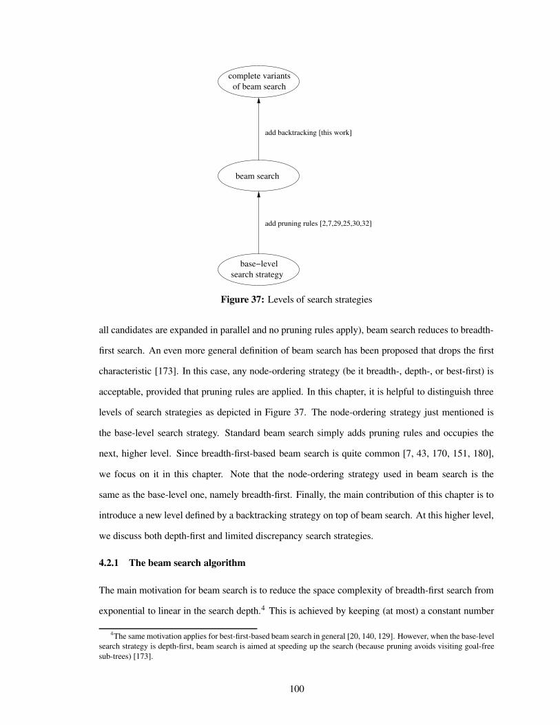
add pruning rules [2,7,29,25,30,32]
of beam search
base−levelsearch strategy
beam search
add backtracking [this work]
complete variants
Figure 37: Levels of search strategies
all candidates are expanded in parallel and no pruning rules apply), beam search reduces to breadth-
first search. An even more general definition of beam search has been proposed that drops the first
characteristic [173]. In this case, any node-ordering strategy (be it breadth-, depth-, or best-first) is
acceptable, provided that pruning rules are applied. In this chapter, it is helpful to distinguish three
levels of search strategies as depicted in Figure 37. The node-ordering strategy just mentioned is
the base-level search strategy. Standard beam search simply adds pruning rules and occupies the
next, higher level. Since breadth-first-based beam search is quite common [7, 43, 170, 151, 180],
we focus on it in this chapter. Note that the node-ordering strategy used in beam search is the
same as the base-level one, namely breadth-first. Finally, the main contribution of this chapter is to
introduce a new level defined by a backtracking strategy on top of beam search. At this higher level,
we discuss both depth-first and limited discrepancy search strategies.
4.2.1 The beam search algorithm
The main motivation for beam search is to reduce the space complexity of breadth-first search from
exponential to linear in the search depth.4 This is achieved by keeping (at most) a constant number
4The same motivation applies for best-first-based beam search in general [20, 140, 129]. However, when the base-levelsearch strategy is depth-first, beam search is aimed at speeding up the search (because pruning avoids visiting goal-freesub-trees) [173].
100

layer 0 = start state
layer 1
layer 2
layer 3
layer 4
layer 5
layer 6
layer 7
layer 0 = start state
layer 1
layer 2
layer 3
layer 4
layer 5
layer 6
layer 7
layer 0 = start state
layer 1
layer 2
layer 3
layer 4
layer 5
layer 6
layer 7
slice 1
slice 1
slice 2
slice 1
slice 1
slice 1 slice 2 slice 3
slice 1 slice 2 slice 3
slice 2 slice 3
slice 2 slice 3
slice 4
slice 4
slice 4
slice 5
slice 5
b) Beam search
a) Breadth−first search
G
G
G
slice 6
B
c) Depth−first beam search
Figure 38: From breadth-first search to beam search to depth-first beam search
101

of nodes at each level in the search tree and pruning all additional nodes. is the size (or
bandwidth) of the beam. Pruned nodes are those in excess of with the worst heuristic values.
Thanks to this pruning mechanism, the space complexity of beam search is É�%© � , , where�
is the
maximum search depth. Figure 38 illustrates the memory requirements (shaded areas) of breadth-
first search (a) and beam search (b). In the figure, the search tree is built from the top down, starting
in the start state. In breadth-first search, each layer is fully generated and stored in memory before
the one below it. Thus, in the worst case, the full search tree is stored down to the depth of the goal
state. The space complexity of breadth-first search is É�%:« º , , where « is the branching factor. In
beam search, each layer is split into slices containing at most nodes. During the search, the set
of nodes at the current level is limited to a single slice. The next layer is generated, that is the set
of successor nodes of the current slice (not the whole layer). Then the nodes in the next layer are
ordered according to increasing heuristic values (from left to right in the figure) and the layer is split
into slices. Only the best (i.e., leftmost slice) is stored in memory and becomes the current layer at
the next level.
Figure 39 contains the pseudo-code for beam search. Beam search takes as an input param-
eter. First, it initializes the hash table and the beam with the start state (Lines 2-3). Then it iterates
on the main loop (Lines 4-22) until 1) the beam is empty, in which case no solution was found
(Line 23), 2) a goal is generated for the first time (Line 8), or 3) the memory is full (Line 20).
At each iteration, the set of all successors of states in the beam is built (Lines 5-11), the beam is
reinitialized (Line 12) and the search depth is incremented by one (Line 13). Finally, the beam is
filled up at the next (deeper) search level (Line 14-21): Until the beam is filled to capacity or there
are no more successors to add (Line 14), the best successor is selected (Line 15), removed from the
set of successors (Line 16), and added to the hash table (Line 18) and the beam (Line 19), provided
it is not already in the hash table (Line 17). In effect, beam search expands all of the nodes in the
beam, orders them according to increasing heuristic values, and adds the new ones in order into the
next-level beam.
Finally, we examine the behavior of beam search under two extreme conditions defined by the
bounding values for .
When $� � , beam search reduces to greedy search since it always expands next the newly
102
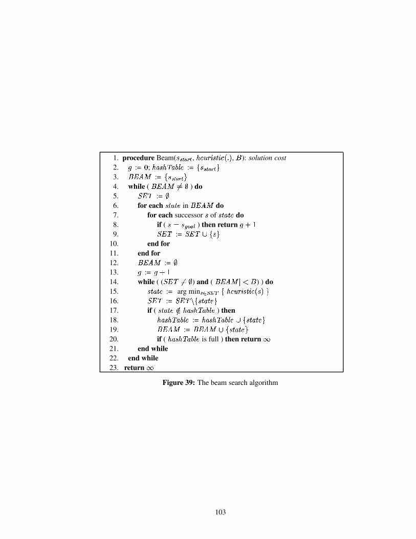
1. procedure Beam( :�36587�9:5 , ;A<J>K@"BED"F6B:G�%¨P�, , ): solution cost2. � := m ; ;K`yD�;¬S�`��J8< := M�:H36587�9:54T3. £XVq®$N := M�:H365I7 9:5¨T4. while ( £*Vq®$N ��¨[ ) do5. WAV1S := [6. for each D"Fa`TFb< in £*VO®§N do7. for each successor : of D"Fa`HFb< do8. if ( :ª�":<xcy ubz ) then return �ª� �9. W=V�S := WAV�S�k M�:@T
10. end for11. end for12. £*VO®§N := [13. � := �ª� �14. while ( ( WAV1S���_[ ) and ( st£*VO®§N%sano ) ) do15. D"Fa`TFb< := arg min r+£Tw?v¯hJM§;A<?>A@"B|D?F6B6Ga%�:�,GT16. WAV�S := WAV�S$j�MTD"Fa`TFb<�T17. if ( D"Fa`TFb< �7°;A`yD�;ZSd`��J8< ) then18. ;K`+D�;ZSd`��?±< := ;A`yD�;ZSd`��J8<¤k MTD"Fa`TFb<�T19. £*VO®§N := £*Vq®$N²k�MTD"Fa`TFb<�T20. if ( ;K`+D�;ZSd`��?±< is full ) then return q21. end while22. end while23. return q
Figure 39: The beam search algorithm
103

generated successor of the current node with the smallest heuristic value. Greedy search may exhibit
poor solution quality when the heuristic function is misleading. It may even become stuck in a dead-
end where the current node has no new successor.
When ���q , beam search behaves like breadth-first search since the beam, as large as the
largest layer, contains all newly generated nodes at the next level. Breadth-first search is guaranteed
to find a minimum-cost path (assuming that all edge costs in the search space are equal, which we
assume throughout this chapter). Unfortunately, due to its exponential space requirements, it may
run out of memory before doing so.
4.2.2 Motivation for backtracking beam search
The foregoing description of beam search naturally creates the following expectations concerning
its behavior.
k For small values of , beam search may terminate without a solution because the beam
becomes empty when the current node has no new successors.
k As increases, beam search finds solutions of higher quality but also uses more and more
time and memory.
k As increases even more, beam search may terminate without a solution because memory
fills up before a goal is found.
Table 17 contains the performance data for beam search averaged over the 50 random instances
of the 48-Puzzle used in Chapter 3. These data essentially exhibit the expected trends. For small
values of (namely 1 and 2), beam search solves none of the instances (see last column). For
larger values of (up to 10,000), beam search solves at least some instances, and the solution cost
generally decreases as increases, while the space usage and the runtime follow an opposite trend.
Finally, when is larger than 10, beam search becomes incomplete (that is, it does not solve 100
percent of our instances) again due to memory shortages.
In addition to confirming our expectations, the data underscore two somewhat surprising and
complementary features. First, the solution quality exhibited by beam search for large values of is
quite high since the average solution cost over solved instances is on the order of 400. This is about
104

Table 17: Performance of beam search in the 48-Puzzle Solution Generated Stored Time Percent
Cost Nodes Nodes (Seconds) Solved1 N/A N/A N/A N/A 02 N/A N/A N/A N/A 03 121,766.68 938,369 365,298 0.615 1004 24,518.68 247,744 98,071 0.161 1005 11,737.12 147,239 58,680 0.090 1006 22,019.68 323,566 132,110 0.208 1007 22,085.92 387,919 154,591 0.250 1008 19,463.92 391,254 155,699 0.264 1009 21,804.96 483,132 196,229 0.309 10010 36,281.64 904,632 362,799 0.601 10020 32,879.92 1,655,928 657,549 1.136 9630 33,732.74 2,561,703 1,011,897 1.879 9440 24,936.02 2,524,773 997,315 1.944 9450 25,341.44 3,211,244 1,266,902 2.495 8660 24,635.84 3,743,041 1,477,936 2.995 9070 19,537.37 3,469,959 1,367,356 2.727 9280 11,908.16 2,411,950 952,341 1.843 8690 12,978.54 2,966,322 1,167,713 2.220 92
100 12,129.88 3,079,594 1,212,579 2.296 86200 6,266.98 3,176,821 1,252,423 2.349 82300 3,469.15 2,625,067 1,039,169 1.890 82400 3,906.33 3,950,665 1,560,311 3.156 78500 2,302.86 2,899,765 1,148,559 2.205 74600 2,161.64 3,263,774 1,293,419 2.524 78700 1,747.58 3,070,222 1,219,046 2.537 90800 1,527.50 3,059,038 1,216,990 2.484 72900 1,448.03 3,261,173 1,297,485 2.747 76
1,000 1,337.95 3,346,004 1,331,451 2.822 842,000 747.02 3,676,719 1,479,593 3.448 943,000 612.42 4,491,479 1,814,334 4.314 864,000 527.88 5,131,180 2,079,790 4.746 805,000 481.30 5,814,061 2,365,603 5.500 866,000 466.49 6,750,775 2,748,609 6.591 827,000 449.67 7,588,757 3,087,861 7.662 868,000 438.52 8,437,526 3,438,717 8.660 809,000 443.27 9,588,420 3,910,897 10.132 88
10,000 440.07 10,569,816 4,312,007 11.307 8020,000 N/A N/A N/A N/A 0
105

an order of magnitude smaller than the solution cost output by the best algorithms in Chapter 3.
Second, and even more surprisingly, the success rate (see last column) remains high (around 80
percent) even for these large values of . This means that beam search with a relatively large value solves a majority of instances with a high solution quality and only runs out of memory in a
small number of cases. This observation is the motivation for our research question: how to make
beam search complete for large values of ? In this chapter, we consider one possible answer,
namely backtracking search.
4.3 Backtracking beam search
The foregoing discussion shows that, at least in one large domain, beam search can use a relatively
wide beam to find high quality solutions in most instances. Assuming that the beam is not so large
that it cannot reach the goal depth, the reason beam search fails to find a goal in a few instances is
that the heuristic values are misleading. For example in Figure 38(b), the goal is mistakenly ordered
in the third slice of the seventh layer. Since beam search only visits the first slice of each layer, it
misses the goal.5 Figure 38(c) illustrates one possible solution to this problem: if the goal is not
found when the search bottoms out, why not backtrack to a previous choice point where the slices
may have been mistakenly ordered?
In this section, we describe two new algorithms. First, we introduce a depth-first extension
of beam search called DB. Then we describe an existing, alternative backtracking strategy called
limited discrepancy search which we use in our new BULB algorithm.
4.3.1 The depth-first beam search (DB) algorithm
The DB algorithm is an extension of beam search that continues the search when it bottoms out
because the memory is full. Before moving back to an earlier choice point in the search tree in order
to explore, for example, the second slice in the next layer, some empty space must be recovered in
memory (since it is now full). The easiest way to do this is to purge one slice and to replace it with
the new one. When it comes to choosing which stored slice to purge, there are as many options
as there are levels in the current path through the search tree. This section discusses the simplest
5Since beam search stops when a goal is generated, this example assumes that the third slice of layer 7 is not asuccessor layer of the first slice of layer 6.
106

choice, namely purging the lastly inserted slice. This strategy is called chronological backtracking
and results in a depth-first extension of beam search which we call DB (for Depth-first Beam search).
Note that heuristic search algorithms that repeatedly fill up and then purge memory are often quite
complicated [19, 143, 86, 177].6 In contrast, because 1) DB uses a depth-first search strategy, 2)
DB always purges contiguous regions of memory and 3) DB does not need to ensure optimality of
the solution, its implementation is (relatively) easy. We now describe DB in detail.
Figure 40 contains the pseudo-code for the depth-first beam search (DB) algorithm. The code
contains four functions: the top-level DB() function and three component functions. We first discuss
the component functions in a bottom-up order, and then the top-level function.
The generateNewSuccessors() function (Lines 30-38) takes as input a set of states and a heuristic
function. It returns an array of all the successors of the input states in order of increasing heuristic
values. The output array only contains newly generated states (i.e., states that are not already in the
hash table). Note that the output array may contain duplicate states since two (or more) states in the
input set may share a newly generated successor. This function does not have any side effects.
The nextSlice() function (Lines 14-29) takes as input the current search depth and the index of
the needed slice at the next level (as well as a heuristic function and the value of ). It is assumed
that the (non-empty) slice at the current level is already in the hash table. This function calls the
preceding one to generate all of the successors of the current slice (Line 16) and it locates the needed
slice within the complete set of successors (Lines 19-28) and returns it (Line 29). As a side effect,
the slice is inserted one successor node at a time into the hash table (Line 23) before the function
returns. The main loop of this function (Lines 19-28) fills up the slice: Starting at startIndex with
an empty slice (Line 19), it iterates over the index into the array SUCCS of successors (Line 27)
until the end of the layer is reached or the slice is filled to capacity, that is (Line 20). Each newly
generated successor (Line 21) is inserted into the slice (Line 22) and the hash table (Line 23). If
the hash table happens to fill up during the processing of the slice (Line 24), the function aborts
(Line 26), but only after having cleared the hash table of the incomplete slice (Line 25).7
6The difficulty lies mainly in the need to maintain 1) the network of data structures (including for example an array ofstates for the hash table and one or more linked lists of states for buckets and other ordered lists) in a coherent state, and2) a set of counters for insuring that the search is admissible.
7This must be done since the calling function (namely DBprobe()) assumes that either the search must continue and thefull slice at the next level is in memory or that the search must backtrack and the memory was not changed in nextSlice().
107

1. procedure DB( Ö ×©ØZÙtÚ'Ø , Û�Ü+Ý@Þ4ßXà4á0ß�â<ãtä å , ³ ): solution cost
2. é ãjÖ ×�ØXÙtÚ'Ø å := ê ; Û{ùQà³Û�(aù�´�µ�Ü := ð?Ö ×�ØXÙtÚ'بñ3. return DBprobe( 0, Û{ÜcÝ@Þ4ßXàwá0ß�â�ã'ähå , ³ )
4. procedure DBprobe( ¶<Ü:·�áIÛ , Û{ÜcÝ@Þ4ßXàwá0ß�â�ã'ähå , ³ ): solution cost
5. à4á�ùQÞ4á8¸�¹K¶�Ü�º := ê6. while ( ájÞ4Ý�Ü ) do7. »�ô{ó¸Qò�î½¼�¾QùJµ Ý�Ü&¼+à4á�ùQÞ4á8¸�¹A¶<Ü/ºK¿ := nextSlice( ¶<Ü:·�áIÛ , à4á�ùQÞ4á8¸�¹A¶<Ü/º , Û{ÜcÝ@Þ4ßXàwá0ß�â�ã'ähå , ³ )
8. if ( ¾?ù�µ Ý�Ü�À�ê ) then return ¾QùJµ Ý�Ü9. if ( ô@ó�¸Qò�î ø ö ) then continue
10. â0Á?à4á := DBprobe( ¶<Ü:·�áIÛ��� , Û�Ü+Ý@Þ4ßXà4á0ß�â<ãtä å , ³ )11. for each Ö in ô@ó¸3ò�î do Û{ù?à³Ûd(�ù&´ µ�Ü := Û{ù?à³Ûd(�ù&´ µ�Ü&��ð?Ö ñ end for12. if ( â/ÁQà4áÂ�°� ) then return â0Á?à4á13. end while
14. procedure nextSlice( ¶�Ü6·�áZÛ , à4á�ùQÞ4á8¸�¹K¶�Ü�º , Û{ÜcÝ@Þ4ßXà4ájß�â�ã'ähå , ³ ): » array of states, integer, integer ¿15. âcÝ@Þ4Þ³Ü�¹�áIó�ù�Ã<Ü+Þ := ð?Ö � Û{ùQà³Û�(aù�´�µ�Ü$)cé ãjÖ?å ø ¶�Ü6·�áZÛ ñ16. ôÅÄAò2ò�ô := generateNewSuccessors( â+Ý@Þ4Þ³Ü�¹�áIó>ùJÃ<ÜcÞ , Û{ÜcÝ@Þ4ßXà4ájß�â�ã'ähå )17. if ( ( ô¯ÄAò2ò�ô ø ö ) or ( àwá�ùQÞ4á8¸�¹A¶<Ü/º ø )hôÅÄAò2ò�ôÂ) ) ) then return »jöT¼��°¼CÆi"¿18. if ( Ö?Ç�È ÙbÉ � ô¯ÄAò2ò�ô ) return »jöT¼?¶<Ü:·�áIÛ$���¼CÆi"¿19. ô{ó¸Qò�î := ö ; Ê := àwá�ùQÞ4á8¸�¹A¶<Ü/º20. while ( ( Ê]��) ô¯ÄAò2ò�ôË) ) and ( ) ô@ó¸3ò�î½)+�,³ ) ) do21. if ( ô¯ÄAò2ò�ôÂÌ Ê�ÍÂ�� Û{ù?à³Ûd(�ù&´ µ�Ü ) then22. é ã�ôÅÄAò2ò�ôÂÌ Ê�ÍZå := ¶�Ü6·�áZÛ ; ô@ó�¸Qò�î := ô@ó�¸Qò�îÎ�¸ð<ô¯Ä)ò2ò>ôËÌ Ê�Í ñ23. Û�ù?à³Û�(aù�´�µ�Ü := Û�ù?à³Û�(aù�´�µ�ÜÏ��ð<ôÅÄAò2ò�ôÂÌ ÊEÍ ñ24. if ( Û�ù?à³Û�(aù�´�µ�Ü is full ) then25. for each Ö in ô@ó�¸Qò�î do Û{ùQàtÛd(�ù&´ µ Ü := Û{ùQàtÛd(�ù&´ µ Ü���ðQÖ ñ end for26. return »0öT¼��°¼CÆi"¿27. Ê := Ê=�°28. end while29. return »'ô@ó�¸Qò�CÆi�¼bÊa¿30. procedure generateNewSuccessors( à4á�ùQá�Ü4ô Ü+á , Û{ÜcÝ@Þ4ßXà4ájß�â�ã'ähå ): array of states
31. ß8¹A¶<Ü/º := ê32. for each à4á�ùQá�Ü in à4á�ùQá�Ü4ô Ü+á do33. for each successor Ö of àwá�ùQá�Ü do34. if ( Ö��� Û�ù?à³Û�(aù�´�µ�Ü ) then ô¯Ä)ò)ò�ôÅÌ�ß8¹K¶�Ü�º4Í := Ö ; ß8¹A¶<Ü/º := ß8¹A¶<Ü/º§��35. end for36. end for37. Sort states in ôÅÄAò2ò�ô in order of increasing Û{ÜcÝ@Þ4ßXà4ájß�â�ã'ähå -values
38. return ô¯Ä)ò2ò>ôFigure 40: The depth-first beam search (DB) algorithm
108

This function returns a 3-tuple containing the output slice, a flag value, and the index of the
following slice to be processed in the next layer. In the normal case (i.e., when the search must
continue down the tree from the slice), the flag value equals negative one. However, there are four
situations under which this function terminates with a positively-valued flag. All indicate that the
search need not continue down the tree below the slice, namely:
k When the set of successors is empty8 (Line 17);
k When the slice index has gone beyond the last slice9 (Line 17);
k When the goal is found in the set of successors (Line 18); or
k When the hash table is full (Lines 24-26).
In all four cases, the returned flag is set to a positive value, that is either the solution cost (in the
third case) or infinity (in the three other cases). In addition, the returned slice index is irrelevant in
all four cases so we arbitrarily set it to negative one.
The DBprobe() function (Lines 4-13) takes as input the current search depth (as well as a heuris-
tic function and the value of ). It repeatedly calls the preceding function to generate a new slice at
the next level and then recursively calls itself to search the sub-tree below the slice. This is where
the chronological backtracking occurs. This function returns a positive value, namely either the cost
of the solution found in the sub-tree rooted at the current slice, or infinity.
This function assumes that the slice at the current search depth is already in the hash table and
it iterates over the slices at the next layer (Lines 5-13). It calls the previous function to load the next
slice into memory (Line 7). If the returned flag value is positive, the search has bottomed out. It
returns either the solution cost or infinity (Line 8). Otherwise (i.e., the value of the flag is negative
one), the search proceeds down the tree, unless the returned slice turns out to be empty (Line 9).
If not, the slice was loaded into memory by nextSlice() and DBprobe() recursively calls itself on
this slice at the next level (Line 10). Upon return, the slice is purged from memory (Line 11) and
8This case arises when all of the successors of the current slice are already in the hash table. This is a dead-end forthe search,
9This is the normal termination condition when the sub-tree under the current slice has been fully searched.
109

the search proceeds with the sibling slice at the current level, unless the goal was found under the
current one (Line 12).
Finally, DB() is the top-level function. It takes as input the start state (as well as a heuristic
function and the value of ) and returns the cost of a solution (or infinity if none was found).
After initializing the hash table with the start state (Line 2), it simply calls DBprobe() at depth zero
(Line 3).
4.3.2 Limited discrepancy search
While using backtracking to transform beam search into a memory-bounded algorithm solves the
memory consumption problem on large instances, is chronological backtracking the most efficient
way to do it in terms of runtimes? [61] observes that the chronological backtracking used in depth-
first search always revisits its most recent decisions (at the bottom of the tree) before it revisits
earlier decisions (at the top of the tree). Since the number of alternatives is exponentially larger at
the bottom than at the top of the tree, it takes a long time before it comes back on an early decision.
In effect, chronological backtracking puts more trust (or weight) in its early decisions than in its later
ones. This is unfortunate because heuristic evaluations are usually more accurate in the proximity
of the goal, that is, they are more likely to be inaccurate at the top of the search tree. So, if the
algorithm makes a wrong decision at the top of the tree and chooses to explore a large, goal-free
sub-tree, depth-first search will waste a lot of time in this sub-tree before it switches to another
sub-tree. Our experiments with DB confirm this analysis (see Section 4.4): DB only improves on
the solution quality of beam search at the cost of unacceptable runtimes. In this section, we propose
to use an existing alternative backtracking strategy called limited discrepancy search which we first
describe in its original version and then generalize to graphs.
4.3.2.1 Original limited discrepancy search
[61] proposes a new backtracking algorithm that weighs equally decisions at all depths of the tree.
Limited discrepancy search (LDS) assumes that the heuristic ordering of successors is right most of
the time. First, LDS searches the tree greedily (that is, with no discrepancy). If no goal is found, it
is because (a presumably small number of) wrong turns were made. Thus LDS iteratively searches
the tree with an increasing number of allowed wrong turns (or discrepancies). Figure 41 depicts
110

1
12345678910111213141516
11 10 8 7 6 5 4 3 2 19
5 4 3 12
no discrepancy1st iteration:
2nd iteration:at most one discrepancy
3rd iteration:at most two discrepancies
4th iteration:at most three discrepancies
5th iteration:at most four discrepancies
15 14 13 12
11 10 8 7 69
12345
Figure 41: Behavior of original limited discrepancy search (LDS) on a balanced, binary tree
111

1. procedure LDS( :43�587�9:5 , ;A<?>A@"B|D?F6B6Ga%¨P�, ): solution cost2. Ð1¢+BED?G�@�</ÑA`+¡dG�B:<?D := m3. while ( F6@">�< ) do4. G� +D"F := LDSprobe( :�36587�9:5 , 0, Ð1¢+B|DJGJ@ <�ÑA`T¡dGJBa<"D , ;A<?>A@"B|D?F6B6Ga%¨P�, )5. if ( G� +D"F¾n9q ) then return G� yD?F6. Ð1¢+B|DJGJ@ <�ÑA`T¡dGJBa<"D := Ð�¢TB|DJGJ@ <�ÑA`+¡ GJBa<"D � �7. end while
8. procedure LDSprobe( D"Fa`TFb< , ¢�<�Ñ F�; , Ð1¢+BED?GJ@ <�Ñ=`+¡dGJBa<"D , ;=<?>A@CBED"F6B:G�%¨P�, ): solution cost9. if ( D?Fa`TFb< is a leaf ) then return q
10. else Ò ��<"D?F?(?DJ<�G� +¡d¢ Ó := generateSuccessors( D?Fa`HFb< )11. if ( ( ��<?D"F �":+Ô Õ 7�Ö ) or ( DJ<�G� +¡d¢8��:yÔ�Õ 7�Ö ) ) then return ¢4<�Ñ F�; � �12. if ( Ð1¢+BED?GJ@ <�Ñ=`+¡dGJBa<"D���m ) then return LDSprobe( ��<?D"F , ¢�</Ñ F�; � � , m , ;A<J>K@"BED"F6B:G�%¨P�, )13. else14. G� yD?F := LDSprobe( D�< G� T¡d¢ , ¢4<�Ñ F�; � � , Ð1¢+BED?G�@�</ÑA`+¡dG�B:<?D Áo� , ;A<J>A@CBED"F6B:G�%¨P�, )15. if ( G� +D"F¾n9q ) then return G� yD?F16. return LDSprobe( �C<"D"F , ¢�<�Ñ F�; � � , Ð1¢+BED?G�@�</ÑA`+¡dG�B:<?D , ;A<J>K@"BED"F6B:G�%¨P�, )
Figure 42: The original limited discrepancy search (LDS) algorithm (for balanced binary trees)
this behavior. LDS is designed to work on finite binary trees. In the figure, the children of each
node are ordered from left to right by increasing heuristic values. So the heuristic function always
recommends going down the left branch while going down the right branch is a wrong turn (or
discrepancy) according to the heuristic. The first iteration is a greedy search with no discrepancy. In
general, the � s � iteration allows for at most � Á8� discrepancies. Within each iteration, discrepancies
occur first at the top of the tree, then further down. Numbers at the bottom of each sub-figure indicate
the order in which leaf nodes are visited during the iteration.
Figure 42 contains the pseudo-code for LDS. The top-level function LDS() repeatedly performs
a limited discrepancy search from the start state (Line 4) by calling LDSprobe() with an increasing
number of allowed discrepancies (Line 6), starting with no discrepancy (Line 2). Unless the current
node is a leaf of the tree (Line 9), LDSprobe() generates its successors and recursively calls itself
on them. If the maximum number of allowed discrepancies is zero, then only the sub-tree below the
best successor is visited with no discrepancy allowed (Line 12). Otherwise, the sub-tree under the
worst successor is visited with one less discrepancy allowed (since one was just consumed, Line 14),
then the sub-tree under the best successor is visited with the same number of allowed discrepancies
(since none was consumed at the current level by following the heuristic recommendation, Line 16).
LDS stops when the goal is generated (Line 11).
112
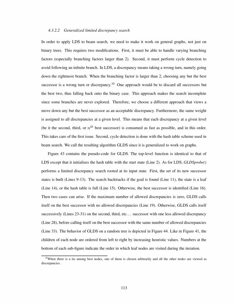
4.3.2.2 Generalized limited discrepancy search
In order to apply LDS to beam search, we need to make it work on general graphs, not just on
binary trees. This requires two modifications. First, it must be able to handle varying branching
factors (especially branching factors larger than 2). Second, it must perform cycle detection to
avoid following an infinite branch. In LDS, a discrepancy means taking a wrong turn, namely going
down the rightmost branch. When the branching factor is larger than 2, choosing any but the best
successor is a wrong turn or discrepancy.10 One approach would be to discard all successors but
the best two, thus falling back onto the binary case. This approach makes the search incomplete
since some branches are never explored. Therefore, we choose a different approach that views a
move down any but the best successor as an acceptable discrepancy. Furthermore, the same weight
is assigned to all discrepancies at a given level. This means that each discrepancy at a given level
(be it the second, third, or � s � best successor) is consumed as fast as possible, and in this order.
This takes care of the first issue. Second, cycle detection is done with the hash table scheme used in
beam search. We call the resulting algorithm GLDS since it is generalized to work on graphs.
Figure 43 contains the pseudo-code for GLDS. The top-level function is identical to that of
LDS except that it initializes the hash table with the start state (Line 2). As for LDS, GLDSprobe()
performs a limited discrepancy search rooted at its input state. First, the set of its new successor
states is built (Lines 9-13). The search backtracks if the goal is found (Line 11), the state is a leaf
(Line 14), or the hash table is full (Line 15). Otherwise, the best successor is identified (Line 16).
Then two cases can arise. If the maximum number of allowed discrepancies is zero, GLDS calls
itself on the best successor with no allowed discrepancies (Line 19). Otherwise, GLDS calls itself
successively (Lines 23-31) on the second, third, etc. . . successor with one less allowed discrepancy
(Line 28), before calling itself on the best successor with the same number of allowed discrepancies
(Line 33). The behavior of GLDS on a random tree is depicted in Figure 44. Like in Figure 41, the
children of each node are ordered from left to right by increasing heuristic values. Numbers at the
bottom of each sub-figure indicate the order in which leaf nodes are visited during the iteration.
10When there is a tie among best nodes, one of them is chosen arbitrarily and all the other nodes are viewed asdiscrepancies.
113
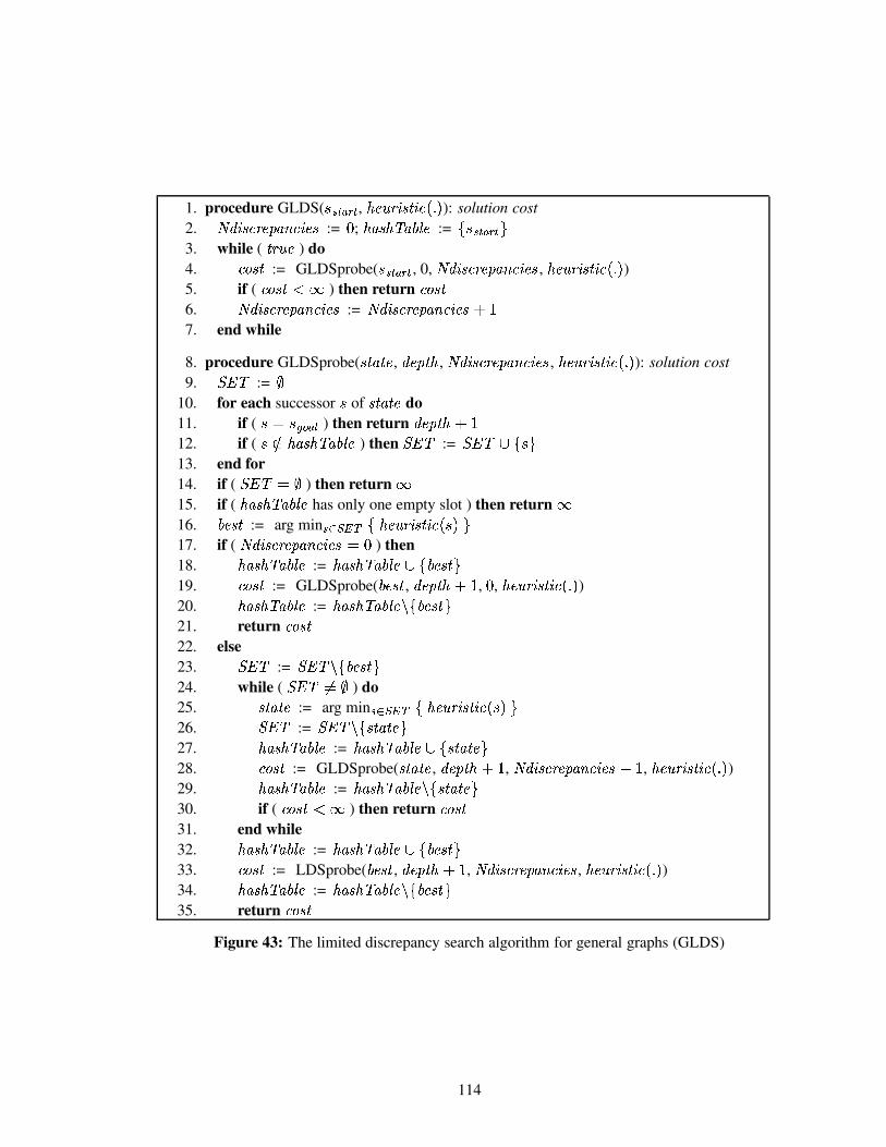
1. procedure GLDS( :4365I7 9:5 , ;A<J>K@"BED"F6B:G�%¨P�, ): solution cost2. Ð1¢+BED?G�@�</ÑA`+¡dG�B:<?D := m ; ;K`yD�;¬S�`��J8< := M�: 36587�9:5 T3. while ( F6@">�< ) do4. G� +D"F := GLDSprobe( :43�587�9:5 , 0, Ð1¢+BED?GJ@ <�Ñ=`+¡dGJBa<"D , ;A<?>A@"B|D?F6B6Ga%¨P�, )5. if ( G� +D"F¾n9q ) then return G� yD?F6. Ð1¢+B|DJGJ@ <�ÑA`T¡dGJBa<"D := Ð�¢TB|DJGJ@ <�ÑA`+¡ GJBa<"D � �7. end while
8. procedure GLDSprobe( D"Fa`HFb< , ¢4<�Ñ F�; , Ð1¢+B|DJGJ@ <�ÑA`T¡dGJBa<"D , ;A<?>A@"B|D?F6B6Ga%¨P�, ): solution cost9. W=V�S := [
10. for each successor : of D"Fa`TFb< do11. if ( :�� :yÔ Õ 7�Ö ) then return ¢�</Ñ F�; � �12. if ( :8�7�;K`yD�;¬S�`��J8< ) then WAV1S := W=V�S.kÄM�:{T13. end for14. if ( WAV1SÐ�¨[ ) then return q15. if ( ;K`+D�;ZSd`��?±< has only one empty slot ) then return q16. �C<"D"F := arg min r+£Tw?v¯hJM¤;A<J>K@"BED"F6B:G�%�:Y,2T17. if ( Ð1¢+BED?GJ@ <�Ñ=`+¡dGJBa<"D���m ) then18. ;K`yDC;ZS�`4�?±< := ;K`yDC;ZSd`��?±<�k�MK�C<"D"FfT19. G� yD?F := GLDSprobe( �C<"D?F , ¢4<�Ñ F�; � � , m , ;=<?>A@CBED"F6B:G�%¨P�, )20. ;K`yDC;ZS�`4�?±< := ;K`yDC;ZSd`��?±<Hj�MK��<?D"FfT21. return G� yD?F22. else23. WAV�S := WAV1S�j�MK��<?D"FfT24. while ( WAV�SF��_[ ) do25. D?Fa`TFb< := arg min r+£Tw?v¯hJM¤;A<?>A@"B|D?F6B6Ga%�:�,GT26. W=V�S := WAV�S$j�MTD"Fa`TFb<�T27. ;A`yD�;ZSd`��J8< := ;K`yDC;ZS�`4�?±<�k�MTD"Fa`TFb<�T28. GC yD"F := GLDSprobe( D"Fa`HFb< , ¢�<�Ñ F�; � � , Ð�¢+BED?G�@�</ÑA`+¡dG�B:<?D Áo� , ;A<J>A@CBED"F6B:G�%¨P�, )29. ;A`yD�;ZSd`��J8< := ;K`yDC;ZS�`4�?±<Tj�MTD"Fa`TFb<aT30. if ( G� yD?F^n9q ) then return GC yD"F31. end while32. ;K`yDC;ZS�`4�?±< := ;K`yDC;ZSd`��?±<�k�MK�C<"D"FfT33. G� yD?F := LDSprobe( �C<"D"F , ¢4<�Ñ F�; � � , Ð1¢+BED?G�@�</ÑA`+¡dG�B:<?D , ;A<?>A@"B|D?F6B6Ga%¨P�, )34. ;K`yDC;ZS�`4�?±< := ;K`yDC;ZSd`��?±<Hj�MK��<?D"FfT35. return G� yD?F
Figure 43: The limited discrepancy search algorithm for general graphs (GLDS)
114
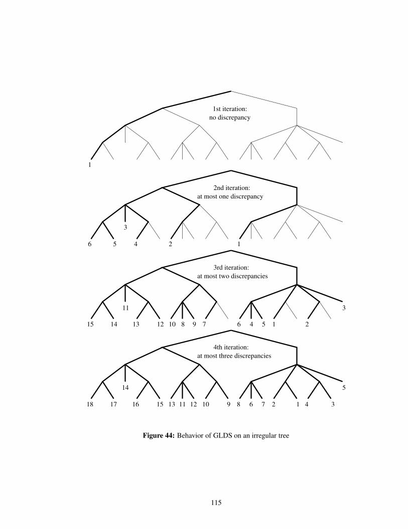
2
12 346 7891011 121315161718
1 24 567981012131415
1st iteration:no discrepancy
2nd iteration:at most one discrepancy
3rd iteration:at most two discrepancies
4th iteration:at most three discrepancies
514
311
3
56 4
1
1
Figure 44: Behavior of GLDS on an irregular tree
115

4.3.3 Beam search using limited discrepancy backtracking (BULB)
Now that we have extended LDS to work on graphs, we can add backtracking based on limited
discrepancy search (instead of chronological backtracking) into beam search. We call the resulting
algorithm BULB (which stands for Beam search Using Limited discrepancy Backtracking).
Figure 45 contains the pseudo-code for BULB. Its top-level function is the same as the one for
GLDS (Lines 1-7 in Figure 43) except that it must initialize the g-value of the start state. The two
bottom-level component functions nextSlice() and storeSuccessors() are the same as the ones for DB
(Lines 14-38 in Figure 40). Only the probe function (renamed BULBprobe()) differs from the one
in both DB and GLDS since it must perform limited discrepancy (not chronological backtracking)
on slices (not on individual states).
The function BULBprobe() starts by generating the first slice at the next level (Line 9). If any
of the four termination conditions shared by DB (see Section 4.3.1) holds, the search has bottomed
out and the function returns either the solution cost or infinity (Line 10). Otherwise, two cases
may arise (like in LDS and GLDS). The first case is when there is no more discrepancy allowed
(Lines 12-15). The search then proceeds to the next level (Line 13) unless the current slice happens
to be empty (Line 12). When the sub-tree rooted in the slice is fully explored, the slice is purged
from memory (Line 14). The second case is when the number of allowed discrepancies is positive
(Lines 17-33). First, the current slice is purged from memory11 (Line 17). Then, BULBprobe() calls
itself recursively on the second, third, etc. . . best slice (Lines 18-27) with one less discrepancy12
(Line 24). Finally, BULBprobe() calls itself recursively on the best slice (Lines 28-33) with the
same number of allowed discrepancies as in the current level (Line 31).
11This is done because, as discussed in Section 4.3.4.1, we enforce an ×*رÙÛÚ�Ü worst-case space complexity. Therefore,we need to regenerate (and order) the slices at each iteration.
12Note that when the search bottoms out for any reason other than having found the goal, the loop should be exited tomove on to the best slice. This is the semantics of the break statement (Line 22). If there is not enough memory to storethis slice, there is not enough memory to store the following slices either. In contrast, when the slice is empty (becauseall of its states are re-generated), this iteration terminates but the remaining slices must still be processed. This is thesemantics of the continue statement (Line 23). In this case, the fact that the current slice is empty does not imply that anyof the remaining slices will be empty. So they must be checked.
116

1. procedure BULB ( Ö3שØZÙtÚ'Ø , Û{ÜcÝ@Þ4ßXàwá0ß�â�ã'ähå , ³ ): solution cost
2. ï�¶3ßXàcâ+Þ³Ü:·�ùJ¹�âcß�Ü+à := ê ; é ãjÖQ×�ØXÙtÚ'Ø'å := ê ; Û{ùQà³Û�(aù�´�µ�Ü := ð?ÖQ×�ØXÙtÚ'Ø ñ3. while ( ájÞ4Ý�Ü ) do4. â/ÁQà4á := BULBprobe( 0, ï$¶QßXàcâ+Þ¨Ü6·�ùJ¹�â+ß�Ü+à , Û{ÜcÝ@Þ4ßXàwá0ß�â�ã'ähå , ³ )
5. if ( â/ÁQà4áÂ��� ) then return â0Á?à4á6. ï�¶QßXàcâcÞ³Ü:·{ù�¹�âcß�Ü4à := ï�¶QßXàcâcÞ³Ü:·{ù�¹�âcß�Ü4àË��7. end while
8. procedure BULBprobe( ¶<Ü:·�áIÛ , ï�¶QßXàcâcÞ³Ü:·{ù�¹�âcß�Ü4à , Û{ÜcÝ@Þ4ßXà4ájß�â�ã'ähå , ³ ): solution cost
9. »�ô{ó¸3òSî½¼�¾QùJµ Ý�Üy¼cà4á©ù3Þ4áI¸ ¹K¶<Ü/ºK¿ := nextSlice( ¶<Ü:·�áIÛ , 0, Û{ÜcÝ@Þ4ßXà4ájß�â�ã'ähå , ³ )
10. if ( ¾?ù�µ Ý�Ü�À�ê ) then return ¾QùJµ Ý�Ü11. if ( ï�¶3ßXà+âcÞ³Ü:·{ù�¹�âcß�Ü4à ø ê ) then12. if ( ô{ó¸3òSî ø ö ) then return �13. â/ÁQà4á := BULBprobe( ¶<Ü:·�áIÛ��� , ê , Û{ÜcÝ@Þ4ßXà4ájß�â�ã'ähå , ³ )
14. for each Ö in ô@ó¸3ò�î do Û�ù?à³Û�(aù�´�µ�Ü := Û�ù?à³Û�(aù�´�µ�Üy��ð?Ö ñ end for15. return â0Á?à4á16. else17. if ( ô{ó¸3òSî�÷ø ö ) then for each Ö in ô{ó¸3òSî do Û�ù?à³Û�(aù�´�µ�Ü := Û�ù?à³Û�(aù�´�µ�Ü&�Yð?Ö ñ end for18. while ( á0Þ4Ý�Ü ) do19. »'ô@ó¸3ò��¾QùJµ Ý�Üy¼+à4á©ù3Þ4áI¸ ¹K¶�Ü�ºK¿ := nextSlice( ¶<Ü:·�áIÛ , à4á©ù3Þ4áI¸ ¹K¶�Ü�º , Û{ÜcÝ@Þ4ßXà4ájß�â�ã'ähå , ³ )
20. if ( ¾QùJµ Ý�Ü�À�ê ) then21. if ( ¾?ù�µ Ý�Ü���� ) then return ¾QùJµ Ý�Ü22. else break23. if ( ô@ó�¸Qò�î ø ö ) then continue24. â0Á?à4á := BULBprobe( ¶<Ü:·�áIÛ��° , ï�¶3ßXà+âcÞ³Ü:·{ù�¹�âcß�Ü4àqÆR , Û{ÜcÝ@Þ4ßXà4ájß�â�ã'ähå , ³ )
25. for each Ö in ô{ó¸Qò�î do Û�ù?à³Û�(aù�´�µ�Ü := Û{ùQà³Û�(aù�´�µ�Ü&�Yð?Ö ñ end for26. if ( â0Á?à4áË�°� ) then return â/ÁQà4á27. end while28. »�ô@ó�¸Qò�C¾?ù�µ Ý�Üy¼+à4á�ùQÞ4á8¸�¹A¶<Ü/º4¿ := nextSlice( ¶�Ü6·�áZÛ , ê , Û{ÜcÝ@Þ4ßXà4ájß�â�ã'ähå , ³ )29. if ( ¾QùJµ Ý�Ü�ÀÄê ) then return ¾?ù�µ Ý�Ü30. if ( ô{ó¸3òSî ø ö ) then return �31. â/ÁQà4á := BULBprobe( ¶<Ü:·�áIÛ��� , ï$¶QßXàcâ+Þ¨Ü6·�ùJ¹�â+ß�Ü+à , Û{ÜcÝ@Þ4ßXàwá0ß�â�ã'ähå , ³ )
32. for each Ö in ô@ó¸3ò�î do Û�ù?à³Û�(aù�´�µ�Ü := Û�ù?à³Û�(aù�´�µ�Üy��ð?Ö ñ end for33. return â0Á?à4á34. procedure nextSlice( ¶�Ü6·�áZÛ , à4á©ù3Þ4áI¸ ¹K¶�Ü�º , Û{ÜcÝ@Þ4ßXà4ájß�â�ã'ähå , ³ ): » array of states, integer, integer ¿35. Same as Lines 15-38 in Figure 40
Figure 45: The BULB algorithm: Beam search using limited discrepancy backtracking
117

Table 18: A taxonomy of beam search methods type of backtracking
none chronological limited discrepancy
1greedy search guided depth-first limited discrepancy search
(gradient descent) search (LDS/GLDS)intermediate beam depth-first beam search beam search using LD backtracking
value search (DB) (BULB)
q breadth-first breadth-first breadth-firstsearch search search
4.3.4 Properties of the BULB algorithm
4.3.4.1 BULB is a memory-bounded algorithm
BULB, like other memory-bounded algorithms [19, 143, 86, 177], continues searching when mem-
ory runs out by purging existing nodes from memory. But what is the space complexity of BULB?
Typically, depth-first search algorithms only need to keep in memory the path from the start state to
the current state, leading to an �% � , complexity, where�
is the maximum search depth. Alterna-
tively, depth-first search with node ordering (sometimes called guided DFS [167]), like BULB (and
DB), also needs to keep in memory the siblings of nodes on the current path, leading to an ɸ%:« � ,complexity, where « is the maximum branching factor. In the case of BULB, like for variants of
beam search, nodes must be stored at each level, leading to a space complexity of either ɸ%© � ,or É�%©Ý« � , . Since BULB uses slice ordering (as in ‘node ordering’), the latter case would typically
hold. However, in order to be able to perform deeper searches with wider beams, we make sure
that the space complexity of BULB does not exceed É�%© � , . This is achieved by only storing one
slice at each level. Therefore, our implementation of BULB must re-generate (and order) all the
successors of a slice every time it backtracks. In Figure 45, the call to nextSlice(), which generates
the whole set of successor slices, is called at the beginning of each iteration. The code uses the
startIndex counter for remembering where the next slice begins in the whole set of successors.
4.3.4.2 BULB generalizes both limited discrepancy search and breadth-first search
BULB is to beam search as LDS is to greedy search since only backtracking need be added to
transform one into the other. Table 18 shows the resulting taxonomy. When � � , slices are
reduced to single states and BULB reduces to (G)LDS. When �� q , slices expand into whole
118

Þ]Þ]Þ]Þ]Þ]Þ]Þ]Þ]Þ]Þ]Þ]Þ]Þ]Þ]Þ]Þ]Þ]Þ]Þ]Þ]Þ]Þ]Þ]Þ]Þ]Þ]Þ]Þ]ÞÞ]Þ]Þ]Þ]Þ]Þ]Þ]Þ]Þ]Þ]Þ]Þ]Þ]Þ]Þ]Þ]Þ]Þ]Þ]Þ]Þ]Þ]Þ]Þ]Þ]Þ]Þ]Þ]ÞÞ]Þ]Þ]Þ]Þ]Þ]Þ]Þ]Þ]Þ]Þ]Þ]Þ]Þ]Þ]Þ]Þ]Þ]Þ]Þ]Þ]Þ]Þ]Þ]Þ]Þ]Þ]Þ]ÞÞ]Þ]Þ]Þ]Þ]Þ]Þ]Þ]Þ]Þ]Þ]Þ]Þ]Þ]Þ]Þ]Þ]Þ]Þ]Þ]Þ]Þ]Þ]Þ]Þ]Þ]Þ]Þ]ÞÞ]Þ]Þ]Þ]Þ]Þ]Þ]Þ]Þ]Þ]Þ]Þ]Þ]Þ]Þ]Þ]Þ]Þ]Þ]Þ]Þ]Þ]Þ]Þ]Þ]Þ]Þ]Þ]ÞÞ]Þ]Þ]Þ]Þ]Þ]Þ]Þ]Þ]Þ]Þ]Þ]Þ]Þ]Þ]Þ]Þ]Þ]Þ]Þ]Þ]Þ]Þ]Þ]Þ]Þ]Þ]Þ]ÞÞ]Þ]Þ]Þ]Þ]Þ]Þ]Þ]Þ]Þ]Þ]Þ]Þ]Þ]Þ]Þ]Þ]Þ]Þ]Þ]Þ]Þ]Þ]Þ]Þ]Þ]Þ]Þ]ÞÞ]Þ]Þ]Þ]Þ]Þ]Þ]Þ]Þ]Þ]Þ]Þ]Þ]Þ]Þ]Þ]Þ]Þ]Þ]Þ]Þ]Þ]Þ]Þ]Þ]Þ]Þ]Þ]ÞÞ]Þ]Þ]Þ]Þ]Þ]Þ]Þ]Þ]Þ]Þ]Þ]Þ]Þ]Þ]Þ]Þ]Þ]Þ]Þ]Þ]Þ]Þ]Þ]Þ]Þ]Þ]Þ]ÞÞ]Þ]Þ]Þ]Þ]Þ]Þ]Þ]Þ]Þ]Þ]Þ]Þ]Þ]Þ]Þ]Þ]Þ]Þ]Þ]Þ]Þ]Þ]Þ]Þ]Þ]Þ]Þ]ÞÞ]Þ]Þ]Þ]Þ]Þ]Þ]Þ]Þ]Þ]Þ]Þ]Þ]Þ]Þ]Þ]Þ]Þ]Þ]Þ]Þ]Þ]Þ]Þ]Þ]Þ]Þ]Þ]ÞÞ]Þ]Þ]Þ]Þ]Þ]Þ]Þ]Þ]Þ]Þ]Þ]Þ]Þ]Þ]Þ]Þ]Þ]Þ]Þ]Þ]Þ]Þ]Þ]Þ]Þ]Þ]Þ]ÞÞ]Þ]Þ]Þ]Þ]Þ]Þ]Þ]Þ]Þ]Þ]Þ]Þ]Þ]Þ]Þ]Þ]Þ]Þ]Þ]Þ]Þ]Þ]Þ]Þ]Þ]Þ]Þ]ÞÞ]Þ]Þ]Þ]Þ]Þ]Þ]Þ]Þ]Þ]Þ]Þ]Þ]Þ]Þ]Þ]Þ]Þ]Þ]Þ]Þ]Þ]Þ]Þ]Þ]Þ]Þ]Þ]ÞÞ]Þ]Þ]Þ]Þ]Þ]Þ]Þ]Þ]Þ]Þ]Þ]Þ]Þ]Þ]Þ]Þ]Þ]Þ]Þ]Þ]Þ]Þ]Þ]Þ]Þ]Þ]Þ]ÞÞ]Þ]Þ]Þ]Þ]Þ]Þ]Þ]Þ]Þ]Þ]Þ]Þ]Þ]Þ]Þ]Þ]Þ]Þ]Þ]Þ]Þ]Þ]Þ]Þ]Þ]Þ]Þ]ÞÞ]Þ]Þ]Þ]Þ]Þ]Þ]Þ]Þ]Þ]Þ]Þ]Þ]Þ]Þ]Þ]Þ]Þ]Þ]Þ]Þ]Þ]Þ]Þ]Þ]Þ]Þ]Þ]ÞÞ]Þ]Þ]Þ]Þ]Þ]Þ]Þ]Þ]Þ]Þ]Þ]Þ]Þ]Þ]Þ]Þ]Þ]Þ]Þ]Þ]Þ]Þ]Þ]Þ]Þ]Þ]Þ]ÞÞ]Þ]Þ]Þ]Þ]Þ]Þ]Þ]Þ]Þ]Þ]Þ]Þ]Þ]Þ]Þ]Þ]Þ]Þ]Þ]Þ]Þ]Þ]Þ]Þ]Þ]Þ]Þ]ÞÞ]Þ]Þ]Þ]Þ]Þ]Þ]Þ]Þ]Þ]Þ]Þ]Þ]Þ]Þ]Þ]Þ]Þ]Þ]Þ]Þ]Þ]Þ]Þ]Þ]Þ]Þ]Þ]ÞÞ]Þ]Þ]Þ]Þ]Þ]Þ]Þ]Þ]Þ]Þ]Þ]Þ]Þ]Þ]Þ]Þ]Þ]Þ]Þ]Þ]Þ]Þ]Þ]Þ]Þ]Þ]Þ]ÞÞ]Þ]Þ]Þ]Þ]Þ]Þ]Þ]Þ]Þ]Þ]Þ]Þ]Þ]Þ]Þ]Þ]Þ]Þ]Þ]Þ]Þ]Þ]Þ]Þ]Þ]Þ]Þ]ÞÞ]Þ]Þ]Þ]Þ]Þ]Þ]Þ]Þ]Þ]Þ]Þ]Þ]Þ]Þ]Þ]Þ]Þ]Þ]Þ]Þ]Þ]Þ]Þ]Þ]Þ]Þ]Þ]ÞÞ]Þ]Þ]Þ]Þ]Þ]Þ]Þ]Þ]Þ]Þ]Þ]Þ]Þ]Þ]Þ]Þ]Þ]Þ]Þ]Þ]Þ]Þ]Þ]Þ]Þ]Þ]Þ]ÞÞ]Þ]Þ]Þ]Þ]Þ]Þ]Þ]Þ]Þ]Þ]Þ]Þ]Þ]Þ]Þ]Þ]Þ]Þ]Þ]Þ]Þ]Þ]Þ]Þ]Þ]Þ]Þ]ÞÞ]Þ]Þ]Þ]Þ]Þ]Þ]Þ]Þ]Þ]Þ]Þ]Þ]Þ]Þ]Þ]Þ]Þ]Þ]Þ]Þ]Þ]Þ]Þ]Þ]Þ]Þ]Þ]ÞÞ]Þ]Þ]Þ]Þ]Þ]Þ]Þ]Þ]Þ]Þ]Þ]Þ]Þ]Þ]Þ]Þ]Þ]Þ]Þ]Þ]Þ]Þ]Þ]Þ]Þ]Þ]Þ]ÞÞ]Þ]Þ]Þ]Þ]Þ]Þ]Þ]Þ]Þ]Þ]Þ]Þ]Þ]Þ]Þ]Þ]Þ]Þ]Þ]Þ]Þ]Þ]Þ]Þ]Þ]Þ]Þ]Þ
ß]ß]ß]ß]ß]ß]ß]ß]ß]ß]ß]ß]ß]ß]ß]ß]ß]ß]ß]ß]ß]ß]ß]ß]ß]ß]ß]ß]ßß]ß]ß]ß]ß]ß]ß]ß]ß]ß]ß]ß]ß]ß]ß]ß]ß]ß]ß]ß]ß]ß]ß]ß]ß]ß]ß]ß]ßß]ß]ß]ß]ß]ß]ß]ß]ß]ß]ß]ß]ß]ß]ß]ß]ß]ß]ß]ß]ß]ß]ß]ß]ß]ß]ß]ß]ßß]ß]ß]ß]ß]ß]ß]ß]ß]ß]ß]ß]ß]ß]ß]ß]ß]ß]ß]ß]ß]ß]ß]ß]ß]ß]ß]ß]ßß]ß]ß]ß]ß]ß]ß]ß]ß]ß]ß]ß]ß]ß]ß]ß]ß]ß]ß]ß]ß]ß]ß]ß]ß]ß]ß]ß]ßß]ß]ß]ß]ß]ß]ß]ß]ß]ß]ß]ß]ß]ß]ß]ß]ß]ß]ß]ß]ß]ß]ß]ß]ß]ß]ß]ß]ßß]ß]ß]ß]ß]ß]ß]ß]ß]ß]ß]ß]ß]ß]ß]ß]ß]ß]ß]ß]ß]ß]ß]ß]ß]ß]ß]ß]ßß]ß]ß]ß]ß]ß]ß]ß]ß]ß]ß]ß]ß]ß]ß]ß]ß]ß]ß]ß]ß]ß]ß]ß]ß]ß]ß]ß]ßß]ß]ß]ß]ß]ß]ß]ß]ß]ß]ß]ß]ß]ß]ß]ß]ß]ß]ß]ß]ß]ß]ß]ß]ß]ß]ß]ß]ßß]ß]ß]ß]ß]ß]ß]ß]ß]ß]ß]ß]ß]ß]ß]ß]ß]ß]ß]ß]ß]ß]ß]ß]ß]ß]ß]ß]ßß]ß]ß]ß]ß]ß]ß]ß]ß]ß]ß]ß]ß]ß]ß]ß]ß]ß]ß]ß]ß]ß]ß]ß]ß]ß]ß]ß]ßß]ß]ß]ß]ß]ß]ß]ß]ß]ß]ß]ß]ß]ß]ß]ß]ß]ß]ß]ß]ß]ß]ß]ß]ß]ß]ß]ß]ßß]ß]ß]ß]ß]ß]ß]ß]ß]ß]ß]ß]ß]ß]ß]ß]ß]ß]ß]ß]ß]ß]ß]ß]ß]ß]ß]ß]ßß]ß]ß]ß]ß]ß]ß]ß]ß]ß]ß]ß]ß]ß]ß]ß]ß]ß]ß]ß]ß]ß]ß]ß]ß]ß]ß]ß]ßß]ß]ß]ß]ß]ß]ß]ß]ß]ß]ß]ß]ß]ß]ß]ß]ß]ß]ß]ß]ß]ß]ß]ß]ß]ß]ß]ß]ßß]ß]ß]ß]ß]ß]ß]ß]ß]ß]ß]ß]ß]ß]ß]ß]ß]ß]ß]ß]ß]ß]ß]ß]ß]ß]ß]ß]ßß]ß]ß]ß]ß]ß]ß]ß]ß]ß]ß]ß]ß]ß]ß]ß]ß]ß]ß]ß]ß]ß]ß]ß]ß]ß]ß]ß]ßß]ß]ß]ß]ß]ß]ß]ß]ß]ß]ß]ß]ß]ß]ß]ß]ß]ß]ß]ß]ß]ß]ß]ß]ß]ß]ß]ß]ßß]ß]ß]ß]ß]ß]ß]ß]ß]ß]ß]ß]ß]ß]ß]ß]ß]ß]ß]ß]ß]ß]ß]ß]ß]ß]ß]ß]ßß]ß]ß]ß]ß]ß]ß]ß]ß]ß]ß]ß]ß]ß]ß]ß]ß]ß]ß]ß]ß]ß]ß]ß]ß]ß]ß]ß]ßß]ß]ß]ß]ß]ß]ß]ß]ß]ß]ß]ß]ß]ß]ß]ß]ß]ß]ß]ß]ß]ß]ß]ß]ß]ß]ß]ß]ßß]ß]ß]ß]ß]ß]ß]ß]ß]ß]ß]ß]ß]ß]ß]ß]ß]ß]ß]ß]ß]ß]ß]ß]ß]ß]ß]ß]ßß]ß]ß]ß]ß]ß]ß]ß]ß]ß]ß]ß]ß]ß]ß]ß]ß]ß]ß]ß]ß]ß]ß]ß]ß]ß]ß]ß]ßß]ß]ß]ß]ß]ß]ß]ß]ß]ß]ß]ß]ß]ß]ß]ß]ß]ß]ß]ß]ß]ß]ß]ß]ß]ß]ß]ß]ßß]ß]ß]ß]ß]ß]ß]ß]ß]ß]ß]ß]ß]ß]ß]ß]ß]ß]ß]ß]ß]ß]ß]ß]ß]ß]ß]ß]ßß]ß]ß]ß]ß]ß]ß]ß]ß]ß]ß]ß]ß]ß]ß]ß]ß]ß]ß]ß]ß]ß]ß]ß]ß]ß]ß]ß]ßß]ß]ß]ß]ß]ß]ß]ß]ß]ß]ß]ß]ß]ß]ß]ß]ß]ß]ß]ß]ß]ß]ß]ß]ß]ß]ß]ß]ßß]ß]ß]ß]ß]ß]ß]ß]ß]ß]ß]ß]ß]ß]ß]ß]ß]ß]ß]ß]ß]ß]ß]ß]ß]ß]ß]ß]ß
à]à]à]à]à]à]à]à]à]à]à]à]à]à]à]àà]à]à]à]à]à]à]à]à]à]à]à]à]à]à]àà]à]à]à]à]à]à]à]à]à]à]à]à]à]à]àà]à]à]à]à]à]à]à]à]à]à]à]à]à]à]àà]à]à]à]à]à]à]à]à]à]à]à]à]à]à]àà]à]à]à]à]à]à]à]à]à]à]à]à]à]à]àà]à]à]à]à]à]à]à]à]à]à]à]à]à]à]àà]à]à]à]à]à]à]à]à]à]à]à]à]à]à]àà]à]à]à]à]à]à]à]à]à]à]à]à]à]à]àà]à]à]à]à]à]à]à]à]à]à]à]à]à]à]àà]à]à]à]à]à]à]à]à]à]à]à]à]à]à]àà]à]à]à]à]à]à]à]à]à]à]à]à]à]à]àà]à]à]à]à]à]à]à]à]à]à]à]à]à]à]àà]à]à]à]à]à]à]à]à]à]à]à]à]à]à]àà]à]à]à]à]à]à]à]à]à]à]à]à]à]à]àà]à]à]à]à]à]à]à]à]à]à]à]à]à]à]àà]à]à]à]à]à]à]à]à]à]à]à]à]à]à]àà]à]à]à]à]à]à]à]à]à]à]à]à]à]à]àà]à]à]à]à]à]à]à]à]à]à]à]à]à]à]àà]à]à]à]à]à]à]à]à]à]à]à]à]à]à]àà]à]à]à]à]à]à]à]à]à]à]à]à]à]à]àà]à]à]à]à]à]à]à]à]à]à]à]à]à]à]àà]à]à]à]à]à]à]à]à]à]à]à]à]à]à]àà]à]à]à]à]à]à]à]à]à]à]à]à]à]à]àà]à]à]à]à]à]à]à]à]à]à]à]à]à]à]àà]à]à]à]à]à]à]à]à]à]à]à]à]à]à]àà]à]à]à]à]à]à]à]à]à]à]à]à]à]à]àà]à]à]à]à]à]à]à]à]à]à]à]à]à]à]à
á]á]á]á]á]á]á]á]á]á]á]á]á]á]á]áá]á]á]á]á]á]á]á]á]á]á]á]á]á]á]áá]á]á]á]á]á]á]á]á]á]á]á]á]á]á]áá]á]á]á]á]á]á]á]á]á]á]á]á]á]á]áá]á]á]á]á]á]á]á]á]á]á]á]á]á]á]áá]á]á]á]á]á]á]á]á]á]á]á]á]á]á]áá]á]á]á]á]á]á]á]á]á]á]á]á]á]á]áá]á]á]á]á]á]á]á]á]á]á]á]á]á]á]áá]á]á]á]á]á]á]á]á]á]á]á]á]á]á]áá]á]á]á]á]á]á]á]á]á]á]á]á]á]á]áá]á]á]á]á]á]á]á]á]á]á]á]á]á]á]áá]á]á]á]á]á]á]á]á]á]á]á]á]á]á]áá]á]á]á]á]á]á]á]á]á]á]á]á]á]á]áá]á]á]á]á]á]á]á]á]á]á]á]á]á]á]áá]á]á]á]á]á]á]á]á]á]á]á]á]á]á]áá]á]á]á]á]á]á]á]á]á]á]á]á]á]á]áá]á]á]á]á]á]á]á]á]á]á]á]á]á]á]áá]á]á]á]á]á]á]á]á]á]á]á]á]á]á]áá]á]á]á]á]á]á]á]á]á]á]á]á]á]á]áá]á]á]á]á]á]á]á]á]á]á]á]á]á]á]áá]á]á]á]á]á]á]á]á]á]á]á]á]á]á]áá]á]á]á]á]á]á]á]á]á]á]á]á]á]á]áá]á]á]á]á]á]á]á]á]á]á]á]á]á]á]áá]á]á]á]á]á]á]á]á]á]á]á]á]á]á]áá]á]á]á]á]á]á]á]á]á]á]á]á]á]á]áá]á]á]á]á]á]á]á]á]á]á]á]á]á]á]áá]á]á]á]á]á]á]á]á]á]á]á]á]á]á]áá]á]á]á]á]á]á]á]á]á]á]á]á]á]á]á
MAXD
Figure 46: From beam search to BULB search
layers and BULB reduces to breadth-first search. The interesting case is the intermediate one since
LDS often terminates without a goal in cyclic graphs (because all successors are being re-generated
and the beam becomes empty) and breadth-first search is too memory-intensive in large state spaces.
BULB occupies this spot.
4.3.4.3 BULB is a complete algorithm
Let NP®$â¤^ denote the maximum depth searchable by both beam search and BULB ( NR®�â¤^ is
approximately equal to ã"�� , where ã is the number of nodes storable in memory).
The main advantage of BULB over beam search is that the latter, because of misleading heuristic
values, may fail to find a goal in some instances where the cost of an optimal path is less than or
equal to NR®�â¤^ . In contrast, BULB is complete over the set of all such instances. This is because
the backtracking mechanism used in BULB makes sure that all successors of the current slice are
potentially generated and expanded if necessary. In other words, BULB is complete because it can
potentially visit the whole NR®�â¤^ -deep search tree rooted at the start state (see Figure 46).
The main advantage of BULB over breadth-first search is that it is complete over a much larger
set of instances, since breadth-first search can only search a significantly smaller tree before it runs
out of memory (the maximum depth searchable by breadth-first search is on the order of �6ä ��å %6ã�, ,
119

a) cycle b) 2 transpositions c) 4 transpositions
Figure 47: Cycles and transpositions
where « is the average branching factor of the search tree).
4.3.4.4 BULB eliminates all cycles and some transpositions
A cycle is a closed loop in the search space (see Figure 47a), while transpositions are distinct paths
between a pair of nodes (see Figure 47b&c).13 Cycles and transpositions are extremely costly if
undetected in depth-first search. Each node (and the sub-tree below it) is searched by depth-first
search as many times as there are paths to it. In a 2D grid for example, while the number of expan-
sions grows quadratically with depth for breadth-first search, it grows exponentially for depth-first
search [162]. Most implementations of depth-first search do not check for duplicates during node
generation. Cycle detection, while easy to perform, consumes valuable runtime. Transpositions are
typically extremely numerous and costly to detect both in terms of runtime and memory usage. This
is why depth-first search is essentially used in tree-like domains [112] or within iterative deepening
search strategies [96]. This discussion also applies to LDS.
Because it is an extension of beam search (which is itself a breadth-first search), BULB auto-
matically eliminates cycles since it saves every expanded node in the hash table and never inserts
13A single cycle is thus part of an infinite number of transpositions.
120
the same state twice in it. On the other hand, BULB does not make any effort at eliminating trans-
positions. Nevertheless, BULB (like beam search) eliminates some transpositions as a by-product
of its memorized beam. For example in Figure 47b, BULB eliminates one of the transpositions to
the bottom node since they both fit completely in the beam of width two (shaded area). However in
Figure 47c, regardless of how nodes are ordered at each level, BULB can only eliminate one of the
two redundant paths to the bottom node.
4.4 Empirical evaluation
In this section, we present an empirical study of our variants of beam search in three benchmark
domains: the�
-Puzzle, the 4-peg Towers of Hanoi domain, and the Rubik’s Cube domain. An
overview of these domains and a description of our empirical setup appear in Chapter 3. All of our
experiments in this chapter were performed on a Pentium-IV PC clocked at a 2.2 GHz with enough
memory to store one or more million nodes (depending on the domain).
4.4.1 Empirical evaluation in the�
-Puzzle domain
4.4.1.1 Evaluation of beam search in the�
-Puzzle
Figure 48 shows the performance of beam search in the�
-puzzle for various values of�
and .
As increases, the solution cost tends to decrease (although the trend is sometimes broken in the
larger puzzles). For all puzzle sizes, the runtime and the number of nodes stored and generated are
strongly correlated. All three measures tend to increase as increases (again, exceptions to this
trend are more numerous for large problem sizes). All these trends confirm our expectations based
on the property that beam search approximates breadth-first search more and more closely as increases. The bottom two graphs illustrate the fact that, in general, obtaining solutions of higher
quality (i.e., lower cost) requires generating and storing more nodes. Of course, it also takes more
time (not shown, since each runtime to solution cost trade-off curve is not significantly different
from the corresponding curve in sub-figure f).
There are three situations in which beam search may terminate without a goal. First, if is
really small (e.g., C�F� or ! in the�
-Puzzle), the beam becomes empty because one of the slices
has no new successors. Solutions to this problem include increasing the value of or finding a better
heuristic function. Second, the shallowest goal may be so deep in the search tree that beam search
121

10
100
1000
10000
100000
1 10 100 1000 10000 100000
Sol
utio
n C
ost (
log
scal
e)
B (log scale)
48-Puzzle35-Puzzle24-Puzzle15-Puzzle8-Puzzle
a) Solution cost versus
0.001
0.01
0.1
1
10
100
1 10 100 1000 10000 100000
Tim
e in
Sec
onds
(log
sca
le)
B (log scale)
48-Puzzle35-Puzzle24-Puzzle15-Puzzle8-Puzzle
b) Runtime versus
100
1000
10000
100000
1e+06
1 10 100 1000 10000 100000
Num
ber o
f Sto
red
Nod
es (l
og s
cale
)
B (log scale)
48-Puzzle35-Puzzle24-Puzzle15-Puzzle8-Puzzle
c) Memory usage versus
100
1000
10000
100000
1e+06
1e+07
1 10 100 1000 10000 100000
Num
ber o
f Gen
erat
ed N
odes
(log
sca
le)
B (log scale)
48-Puzzle35-Puzzle24-Puzzle15-Puzzle8-Puzzle
d) Search effort versus
100
1000
10000
100000
1e+06
10 100 1000 10000 100000
Num
ber o
f Nod
es S
tore
d (lo
g sc
ale)
Solution Cost (log scale)
48-Puzzle35-Puzzle24-Puzzle15-Puzzle8-Puzzle
e) Memory usage versus solution cost
100
1000
10000
100000
1e+06
1e+07
10 100 1000 10000 100000
Num
ber o
f Nod
es G
ener
ated
(log
sca
le)
Solution Cost (log scale)
48-Puzzle35-Puzzle24-Puzzle15-Puzzle8-Puzzle
f) Search effort versus solution cost
Figure 48: Performance of beam search in the�
-Puzzle with varying
122
always runs out of memory before reaching it (i.e., the total memory needed for all nodes in the
beam down to the goal is larger than the available memory). The solution to this problem requires
decreasing the value of . Third, in the intermediate case, beam search runs out of memory at a
given depth (say,�) because the heuristic function leads it astray. Since this situation assumes that
there is a goal at level�
(or higher in the tree), solutions to this problem include finding 1) a better
heuristic function and 2) a memory-purging strategy that continues searching “against” the heuristic
recommendation to find out where it is wrong.
The last two cases are failures due to memory shortages. Yet, they are qualitatively different
from each other. One requires a new (smaller) value for while the other does not. In keeping
with standard practice, we assume that is a constant and focus on the last case. Our approach
to this problem in this chapter is to use backtracking. Unfortunately, chronological backtracking
(implemented in DB) does not solve this problem in a reasonable amount of time. In our experi-
ments, we have not found a problem instance 1) in which beam search fails solely because of the
heuristic ordering of nodes and 2) that is solved by DB in a reasonable amount of time (on the order
of minutes). This illustrates the weakness of chronological backtracking. Thus, we now turn to
discrepancy-based backtracking.
4.4.1.2 Evaluation of BULB in the�
-Puzzle
Our experiments show that beam search has an impressive scaling behavior in the�
-puzzle (it can
solve any random instance of the 48-puzzle in a fraction of a second). For this reason, our negative
results with DB might be due to a ceiling effect (that is, there is not much room for improvement
over beam search by any algorithm). We indeed believe this to be the case, at least for small values
of�
(up to 35). For example, beam search can solve all of our instances of the 35-Puzzle with as large as 22,000. In our setup, the memory can contain up to 6 million nodes, thus the maximum
searchable depth is about 273 ( ���(+m@m@m�(+m@m@m��Y!@!�(+m@m@m ). Given that, with these settings, the average
(respectively, maximum) solution cost in our sample is 226 (respectively, 274), it is possible (and
even likely) that any larger value of will cause beam search to run out of memory on some
instance because the goal is just too deep to reach even with a perfect heuristic function. If this
conclusion really holds, then there is no hope of improving upon beam search in the 35-Puzzle by
123

simply adding backtracking. As a further confirmation of this ceiling effect, our experiments with
BULB (in addition to those with DB) have also not shown any significant improvement over beam
search for� � Ì � (or smaller).
In contrast, the failure of DB to improve on beam search in the 48-puzzle is not the result of a
ceiling effect since BULB can significantly improve on beam search (see Figure 49). The graphs
show the performance of both beam search and BULB in the 48-Puzzle with the same amount of
memory (namely 6 million nodes). Since BULB generates nodes in exactly the same order as beam
search, we plot the performance of both algorithms using a single curve in which BULB’s curve
simply extends the curve of beam search (BULB is complete with much larger values than beam
search). Since BULB is slightly slower than beam search in our recursive implementation of BULB,
only the runtime data are plotted as two curves.
Our results show that, by increasing to much larger values than beam search can handle in
the 48-puzzle, BULB exhibits a 25-fold reduction in the solution cost (from 11,700 for beam search
down to 440 for BULB) but still enjoys reasonable maximum average runtimes on the order of 30
seconds.
4.4.1.3 Comparison with variants of multi-state commitment search
Figure 50 compares the performance of beam search and BULB with that of the best two algorithms
in Chapter 3 in the 48-Puzzle. With the same amount of memory, BULB improves the solution
quality of MSC-KWA* and MSC-KRTA* by about an order of magnitude while keeping the runtime
reasonable (MSC-KWA* and MSC-KRTA* are variants of WA* and RTA*, respectively, whose
behavior is similar to that of beam search).
4.4.1.4 BULB scales up to even larger puzzles
In order to provide additional support for the scaling behavior of BULB, we also report experimental
results for larger puzzles (namely for� � È@Ì and
� �æzYm ). In our empirical setup, while beam
search is not able to solve all fifty random instances in either puzzle size, BULB remains complete
for a large set of values. Figures 51 & 52 show the behavior of BULB in these larger�
-puzzle
domains. On average, BULB solves all instances of the 63- and 80-Puzzle as fast as in about 1
and 10 seconds, respectively. If more time is available to look for better solutions, larger values of
124

1000
10000
100000
1 10 100 1000 10000
Solution cost (log scale)
B (log scale)
beam searchBULB
a) Solution cost versus
0.1
1
10
100
1 10 100 1000 10000
Time in Seconds (log scale)
B (log scale)
beam searchBULB
b) Runtime versus
10000
100000
1e+06
1e+07
1 10 100 1000 10000
Number of Stored Nodes (log scale)
B (log scale)
beam searchBULB
c) Memory usage versus
100000
1e+06
1e+07
1 10 100 1000 10000 100000
Number of Generated Nodes (log scale)
B (log scale)
beam searchBULB
d) Search effort versus
10000
100000
1e+06
1e+07
1000 10000 100000
Number of Stored Nodes (log scale)
Solution cost (log scale)
beam searchBULB
e) Memory usage versus solution cost
100000
1e+06
1e+07
1000 10000 100000
Number of Generated Nodes (log scale)
Solution cost (log scale)
beam searchBULB
f) Search effort versus solution cost
Figure 49: Performance of BULB in the 48-Puzzle with varying
125

0.1
1
10
1000 10000 100000
Time in Seconds (log scale)
Solution Cost (log scale)
MSC-KWA*MSC-KRTA*
beam searchBULB
Figure 50: Comparing the performance of beam search and BULB with that of MSC-KWA* andMSC-KRTA* in the 48-Puzzle with varying
1
10
100
100 1000 10000 100000
Time in Seconds (log scale)
Solution cost (log scale)
BULB
Figure 51: Performance of BULB in the 63-Puzzle with varying (memory = 4 million nodes)
126

10
100
1000 10000 100000
Time in Seconds (log scale)
Solution cost (log scale)
BULB
Figure 52: Performance of BULB in the 80-Puzzle with varying (memory = 3 million nodes)
(5,000 and 20,000, respectively) yield solutions that are on average (as a conservative estimate)
no more than five times larger than optimal (lowest solution costs average about 700 and 1130,
respectively). The average runtimes corresponding to such a high solution quality remain reasonable
(approximately 50 and 120 seconds, respectively).
4.4.2 Empirical evaluation in the Towers of Hanoi domain
Our second benchmark domain is the 4-peg Towers of Hanoi domain (also called the Reve’s Puzzle,
see Section 3.6.2). Our experiments involve fifty random instances with 22 disks in which the goal
state has all disks stacked up on the destination peg (or tower). In our empirical setup, the memory
can store up to one million nodes. In this setup, none of our test values for makes beam search
complete. Interestingly, Table 19 shows a pattern reminiscent of the behavior of beam search in the
48-Puzzle, namely that beam search with large values of solves a large proportion of instances
(about 70 percent) with a high solution quality.
If its superior scaling behavior carries over to this domain, BULB should be able to solve the
remaining 30 percent of instances in which beam search runs out of memory. Figure 53 shows that
this is indeed the case. The shortest average runtime of BULB is about one and a half second. It
is obtained for �/Ç{m and yields an average solution quality of about 10,000. If more time is
127

Table 19: Performance of beam search in the Towers of Hanoi domain (memory = 1 million nodes) Solution Generated Stored Time Percent
Cost Nodes Nodes (Seconds) Solved1 N/A N/A N/A N/A 02 115,704.00 890,027 231,401 0.360 23 130,153.00 1,519,900 390,451 0.633 244 59,836.75 909,528 239,342 0.374 485 37,775.12 730,901 188,860 0.306 686 41,507.95 942,024 249,012 0.432 407 39,229.08 1,030,574 274,588 0.446 508 42,626.67 1,279,381 340,982 0.592 429 34,337.59 1,163,909 309,019 0.522 44
10 33,489.26 1,261,982 334,850 0.581 4620 17,588.28 1,330,487 351,700 0.687 5030 13,414.43 1,531,218 402,270 0.811 7040 9,843.84 1,503,808 393,571 0.799 7650 8,468.59 1,619,300 423,103 0.900 6860 7,073.51 1,625,596 423,951 0.967 8670 6,533.43 1,755,253 456,849 1.005 7080 5,562.51 1,710,901 444,503 0.988 7090 5,189.43 1,798,047 466,470 1.139 74100 4,629.57 1,784,654 462,443 1.012 70200 2,745.81 2,122,040 547,955 1.406 74300 1,948.68 2,261,154 583,020 1.429 76400 1,579.78 2,442,440 629,629 1.714 72500 1,363.59 2,632,408 678,792 1.855 74600 1,172.05 2,712,527 699,411 1.851 76700 1,081.12 2,916,584 752,281 2.104 66800 1,020.78 3,143,096 810,973 2.365 54900 931.00 3,223,097 831,574 2.465 70
1,000 831.90 3,196,242 824,784 2.388 582,000 450.33 3,422,296 883,680 2.930 123,000 N/A N/A N/A N/A 0
128

100
1000
10000
100000
10 100 1000
Sol
utio
n C
ost (
log
scal
e)
B (log scale)
BULB
a) Solution cost versus
1
10
1 10 100 1000 10000
Tim
e in
Sec
onds
(log
sca
le)
B (log scale)
BULB
b) Runtime versus
100000
1e+06
1e+07
10 100 1000
Num
ber o
f Sto
red
Nod
es (l
og s
cale
)
B (log scale)
BULB
c) Memory usage versus
100000
1e+06
1e+07
10 100 1000
Num
ber o
f Gen
erat
ed N
odes
(log
sca
le)
B (log scale)
BULB
d) Search effort versus
100000
1e+06
1e+07
100 1000 10000 100000
Num
ber o
f Sto
red
Nod
es (l
og s
cale
)
Solution Cost (log scale)
BULB
e) Memory usage versus solution cost
100000
1e+06
1e+07
100 1000 10000 100000
Num
ber o
f Gen
erat
ed N
odes
(log
sca
le)
Solution Cost (log scale)
BULB
f) Search effort versus solution cost
Figure 53: Performance of BULB in the Towers of Hanoi domain with varying (memory = 1million nodes)
129

available to look for better solutions, larger values of (say, 1,000) yield solutions of significantly
higher quality (namely, around 870) in very reasonable runtimes (about seven seconds).
4.4.3 Empirical evaluation in the Rubik’s Cube domain
Our third benchmark domain is the Rubik’s Cube. Our experiments involve fifty random instances
in which the goal state is the original configuration of the cube (where each of the six faces is
uniformly colored, see Section 3.6.3). In our empirical setup, where the memory can store up to
one million nodes, several of our test values for make beam search complete (see Table 20).
The lowest average solution cost found by beam search is 55.18. This level of solution quality is
similar to that found by a recent, powerful Rubik’s Cube solver based on macro-operators, even
though the latter uses both a larger number of pattern databases to build the macro-operators and
a post-processing step on solution paths [63]. Therefore, beam search is a strong contender in this
domain.
Nevertheless, BULB improves on beam search since it is complete in this domain over the whole
range of our test values for . Figure 54 shows that the lowest average solution cost (namely 22.74)
found by BULB is reached in about seven minutes for � � m�(+m@m@m . A slightly higher average
solution cost of 25.78 is found by BULB in approximately two minutes for �FÇ{m�(+m@m@m . Finally,
the best average solution cost found by BULB in under a minute (namely about forty seconds)
is 30.14 for ��ÌYm�(+m@m@m (We also ran BULB with ��ÌYm�(+m@m@m and averaged its performance
over 10,000 random instances; Table 21 shows that averaging over this much larger set of instances
yields similar performance.). This solution quality (obtained in less than a minute) is higher than
that of the Rubik’s Cube solver presented in [63]. Therefore, we believe that BULB is a state-of-
the-art solver in this domain (in terms of the trade-off between solution quality and runtime) even
though it is a pure-search (i.e., no pre- nor post-processing), domain-independent algorithm that
uses relatively little memory (about 120 Mbytes in our setup, including about 86 Mbytes for the
three pattern databases used by the heuristic function and about 32 Mbytes for the hash table).
130

Table 20: Performance of beam search in the Rubik’s Cube domain (memory = 1 million nodes) Solution Generated Stored Time Percent
Cost Nodes Nodes (Seconds) Solved10 53,909.26 7,146,960 539,084 14.965 3820 23,343.35 6,184,444 466,846 12.327 6230 9,805.89 3,896,606 294,136 7.911 8840 5,748.60 3,046,073 229,883 6.212 9450 3,882.35 2,570,677 194,036 5.224 9860 3,586.28 2,850,134 215,076 5.819 10070 2,274.94 2,108,661 159,125 4.180 10080 1,978.52 2,095,562 158,141 4.089 10090 1,587.08 1,890,560 142,676 3.676 98100 1,679.76 2,223,466 167,795 4.349 98200 888.76 2,349,712 177,371 4.635 100300 656.06 2,598,820 196,180 5.171 100400 446.08 2,349,595 177,494 4.657 100500 394.84 2,596,065 196,182 5.168 100600 321.72 2,532,990 191,494 5.040 100700 305.02 2,799,796 211,676 5.589 100800 250.92 2,625,262 198,598 5.226 100900 255.58 3,008,772 227,584 6.020 100
1,000 259.80 3,398,726 257,058 6.798 982,000 141.81 3,662,902 277,879 7.389 943,000 103.56 3,969,587 301,942 8.015 1004,000 78.52 3,952,171 301,582 7.975 1005,000 78.02 4,895,297 373,602 9.977 1006,000 70.23 5,244,995 400,877 10.726 967,000 55.18 4,712,217 361,762 9.610 1008,000 56.61 5,531,299 424,400 11.344 989,000 54.41 5,952,781 457,175 12.269 98
10,000 52.33 6,332,050 486,767 13.087 9820,000 37.13 8,580,244 666,111 18.033 9230,000 29.86 9,950,562 779,364 21.124 5840,000 24.42 10,358,637 820,169 22.098 2450,000 21.40 10,848,794 866,741 23.256 1060,000 N/A N/A N/A N/A 0
Table 21: Performance of BULB in the Rubik’s Cube domain averaged over 1,000 random instances(memory = 1 million nodes)
Solution Generated Stored Time PercentCost Nodes Nodes (Seconds) Solved
30,000 30.58 18,029,740 797,275 39.636 100
131

10
100
1000
10000
100000
10 100 1000 10000
Sol
utio
n C
ost (
log
scal
e)
B (log scale)
beam searchBULB
a) Solution cost versus
1
10
100
1000
10 100 1000 10000
Tim
e in
Sec
onds
(log
sca
le)
B (log scale)
beam searchBULB
b) Runtime versus
100000
1e+06
1e+07
1e+08
10 100 1000 10000
Num
ber o
f Sto
red
Nod
es (l
og s
cale
)
B (log scale)
beam searchBULB
c) Memory usage versus
100000
1e+06
1e+07
1e+08
10 100 1000 10000
Num
ber o
f Gen
erat
ed N
odes
(log
sca
le)
B (log scale)
beam searchBULB
d) Search effort versus
100000
1e+06
1e+07
1e+08
100 1000 10000 100000
Num
ber o
f Nod
es S
tore
d (lo
g sc
ale)
Solution Cost (log scale)
beam searchBULB
e) Memory usage versus solution cost
100000
1e+06
1e+07
1e+08
100 1000 10000 100000
Num
ber o
f Nod
es G
ener
ated
(log
sca
le)
Solution Cost (log scale)
beam searchBULB
f) Search effort versus solution cost
Figure 54: Performance of beam search and BULB in the Rubik’s Cube with varying (mem-ory = 1 million nodes)
132

4.5 Related work4.5.1 Band search
Besides beam search itself, the closest existing algorithm to BULB is band search [20]. Band search
is a memory-bounded algorithm that maintains a bounded number of nodes (called a band) at each
level of the search tree, expands these nodes in best-first order, and backtracks when a goal is found
or the band is empty. We first describe the behavior of band search in more detail and then compare
and contrast it with BULB.
Band search (denoted BS(W)) maintains a set (or band) of (at most) active nodes at each
level of the search tree. The nodes are the ones with the lowest f-values at this level and are
ordered according to increasing f-values. Additional nodes are stored in overflow lists, one at each
level. These lists are also internally ordered by increasing f-values. Furthermore, the total set of
active nodes (i.e., the union of the bands, but not the overflow lists, at all levels) is also ordered
by increasing f-values. Finally, a counter is maintained at each level of the search tree to limit the
degree of backtracking allowed. Each counter keeps track of how many nodes have been expanded
at this level.
BS starts with the start state in the band at level 0 (and its counter initialized with a value of
one) and all other lists empty (and all other counters with a value of zero). At each iteration, a node
with the smallest f-value among those in all the bands is selected for expansion and removed from
its band. Its successors are generated and processed as follows. If a successor’s f-value is larger
than or equal to the cost of the best solution found so far (initially equal to infinity), it is pruned. If a
successor is a goal with a lower cost than the best found so far, the latter is updated (i.e., decreased).
Each non-pruned successor is inserted into the band at the next level and its counter is incremented
by one. If the band’s size exceeds , excess nodes with the largest f-values are moved into the
overflow list at this level and the counter is reset to . This process continues until the union of
all the bands is empty. At this point, if all the overflow lists are also empty, the search terminates.
Otherwise, the best nodes in the deepest overflow list are inserted into the band at their level, all
the counters are reset to zero, and the search restarts.
BS( ) is a generalization of both guided depth-first search (GDFS) and best-first search. When
� � , only one node is active at each level, namely the best unexpanded one. In fact, since the
133

expanded node is immediately removed from its band, there is only one non-empty band in the
whole search tree at any time. Therefore, BS(1) searches greedily, that is depth-first on the best
node. When the bands are all empty, the deepest overflow list is used to provide the next starting
point. This enforces the chronological backtracking needed for depth-first search.
When �Oq , all successor nodes are added to the band at the next level. The overflow lists
remain empty. Since BS always chooses for expansion a node with the smallest f-value, BS( q ) is
functionally equivalent to best-first search.
For values of n q , BS can be seen as 1) a best-first version of beam search (which is a
breadth-first search) or 2) a beam-search version of best-first search in which the beam width is
uniform across levels. The main advantage of band search over best-first search is its bounded
memory requirements. By construction, each band cannot contain more than the best nodes.
Furthermore, the overflow list contains the other successors of the nodes in the band at the next
higher level. Thus, each level contains at most � �P�%:« Á��<,����P}« nodes, where « is the
maximum branching factor. Finally, if the maximum search depth is�, the worst-case memory
requirements for BS( ) are ɸ%'�« � , .A related algorithm is Ibaraki’s depth-m search [73] since it simulates best-first search with
bounded memory. However, its memory bound is exponential (more precisely, on the order of
É�% �Kç , , where�
is the maximum search depth).
Similarities between BS and BULB
k Both algorithms are variants of beam search that have a memory bound that is polynomial in
the bandwidth and the maximum search depth.
k Both algorithms reduce to variants of depth-first search when ��� , namely to guided
depth-first search for BS, and to limited discrepancy search for BULB .
k Both algorithms are anytime algorithms since they may keep searching for better and better
solutions after the first one is found.
Differences between BS and BULB
k BS is a variant of best-first search while BULB is a variant of breadth-first search. Further-
more, BS expands one node at a time while BULB expands all nodes at a given level in
134

parallel. In this respect, BULB is more diversified than BS (see Chapter 3 for a discussion of
diversification).
k The memory consumption of BS is higher than that of BULB (by a constant factor of « )because BS stores in memory all successors of the bands at all levels, while BULB only
stores the successors that are actually in the bands. The flip side of this feature is that BULB
must re-generate the discarded successors upon backtracking while BS keeps them in the
overflow lists.
k BS uses chronological backtracking when reaching the bottom of the tree while BULB uses
limited discrepancy search. Since it is more likely that the heuristic function is misleading at
the top of the tree, it seems more fruitful to backtrack there instead of at the bottom of the
tree. Our experiments (with DB) have indeed confirmed this.
k BS is essentially designed to work on trees, like depth-first search. While it can be (and has
been) applied to general graphs, it does not contain any loop-detection mechanism. Therefore,
according to [20], BS “is efficient for solving problems that do not have deep search trees. [...]
It should not be applied to problems [...] such as puzzle and maze problems.” When applied
to graphs such as the�
-puzzle, it must be used in the context of iterative-deepening search.
However in this case, BS can only be useful in the last iteration of IDA* and the improvement
in the 15-puzzle (the largest tested puzzle domain) is small (if any) because the threshold on
the last iteration is typically equal to the optimal cost and BS must expand all nodes reachable
in the last iteration in best-first order.
k Implementing BS is significantly harder than for BULB because BS maintains two ordered
lists at each level (one band and one overflow list). In addition, the set of band lists must also
be threaded into a single list (akin to the OPEN list in A*) ordered by increasing f-values. In
contrast, BULB maintains a single list (namely, the ordered list of nodes at the current level).
In [21], BS is extended in two ways. First, the bandwidth is varied dynamically during
search. It is decreased by one when a goal is found and increased by one when the search bottoms
out without finding a goal. Second, BS is combined with GDFS: The new algorithm performs
135
guided depth-first search to find a first-solution and then switches to BS to refine the first solution.
However, these improvements do not overcome the limitations of BS in general graphs. They are
only evaluated on known, fixed-depth trees (asymmetric TSP problems) and on maze problems
whose search space fits in memory and could be quickly solved optimally by A* or IDA*.
4.5.2 Diversity beam search
Beam search relies on heuristic evaluations to order nodes at each level. When the heuristic function
is misleading, beam search can be led astray. Both BULB and BS tackle this issue using backtrack-
ing. In contrast, [151] presents a variant of beam search (called Diversity Beam Search or DBS) that
does not backtrack. Instead, it introduces diversity into the search at all levels of the tree in order to
increase the quality of the solution found. Diversity is evaluated by an additional function that takes
a set of states and ranks them according to how dissimilar they are. This evaluation is combined with
the heuristic function to decide which nodes to keep at the next level. In [151], increased diversity is
aimed at improving the solution quality. In our context, it would be used to increase the probability
of finding a solution at all before memory runs out. One difficulty with DBS is that it needs an
additional function for measuring dissimilarity. The paper applies the idea to the CRESUS expert
system for intelligent cash management [150]. In general, a good dissimilarity measure is likely to
be domain-dependent and/or hard to find. It should at least statistically beat a trivial approach such
as adding to the beam randomly selected nodes with high heuristic evaluations. Another problem
with DBS is that it does not provide for a backup mechanism when no solution is found. Since
the dissimilarity measure is heuristic in nature, it is likely to lead the search astray in at least some
instances. One possible solution would be to combine the idea of diversity with the backtracking
mechanisms used in BULB or BS.
4.5.3 Complete anytime beam search
[173] takes a very general view of beam search as any search technique that uses pruning rules
to discard non-promising alternatives, regardless of how nodes are ordered for expansion. While
the traditional beam search is based on breadth-first search [7, 43, 170, 151] (including this work),
other variants are based on best-first search [20, 21]. [173] applies the term to a variant of depth-first
search. The idea behind Complete Anytime Beam search (CABS) is to repeatedly call a variant of
136
depth-first search that uses a pruning rule that is progressively weakened at each iteration. One main
contribution of the paper is a new domain-independent pruning rule whose strength is controlled by
a single parameter. As the pruning rule is weakened, fewer and fewer nodes are pruned. In the
worst case, no pruning occurs and thus CABS is complete. The idea of iterative weakening was
introduced in [134]. The particular pruning rule introduced in the paper is similar but different from
the idea of iterative broadening [54]. CABS is shown to be both an optimization algorithm and an
efficient approximation algorithm for the maximum boolean satisfiability problem as well as the
symmetric and asymmetric TSP. Unfortunately, CABS, like most variants of depth-first search, is
only well suited to problems with a high density of solutions or a finite search tree [135].
4.5.4 Variants of discrepancy search
One drawback of LDS [61] is that each iteration allows at most a given number � of discrepancies.
This means that each iteration re-visits all the full paths generated during all previous iterations.
[100] proposes ILDS, an improved version of LDS, that only generates paths with exactly � dis-
crepancies, with � incremented by one at each iteration.14 Unfortunately, ILDS needs one addi-
tional parameter to behave as described, namely the maximum search depth. This is not always
known with precision. To remedy this problem, [169] proposes another variant of LDS, called DDS
for depth-bounded discrepancy search, that also never re-generates full paths but does not need an
upper bound on the search depth. DDS combines the ideas of limited discrepancy search and iter-
ative deepening. At each iteration, DDS does not allow discrepancies below a certain level in the
tree, that is: the m s � iteration allows no discrepancy, the first iteration does not allow discrepancies
below depth 0, the second iteration does not allow discrepancies below depth 1, etc. With an easy
additional mechanism, DDS avoids re-visiting full paths generated during previous iterations.
Conceptually, the evolution from depth-first search, to LDS, to ILDS, and finally to DDS, is best
characterized by the way discrepancies are weighted at different search depths.15
k Depth-first search weighs discrepancies more at the top of the tree. Thus it goes against the
heuristic evaluations (a discrepancy) deep in the tree before it does so toward the top of the
14This property only holds when the tree is balanced and its depth is known exactly.15Since a discrepancy is a move against the heuristic recommendation, a small-weight discrepancy is preferred over a
large-weight one.
137
tree, resulting in chronological backtracking.
k LDS weighs discrepancies equally at all levels of the tree. Its search strategy is based on the
(increasing) number of discrepancies, not their depth in the tree.
k Like LDS, ILDS searches iteratively in order of increasing numbers of discrepancies. But,
like depth-first search, it weighs discrepancies more at the top of the tree.
k DDS (in complete opposition to depth-first search and ILDS) weighs discrepancies in propor-
tion to their depth in the tree. Therefore, it goes against the heuristic evaluations at the top of
the tree before it does so toward the bottom of the tree. This makes sense when the heuristic
function is less accurate at the top of the tree, that is away from the goal.
We have not yet applied DDS in the context of beam search, mainly because in our experiments,
LDS is sufficient to show significant improvement over depth-first search. Nevertheless, since the
DDS strategy may be even more efficient, its application to beam search is part of our plans for future
work. However, we do not plan to implement ILDS since it requires the additional knowledge of an
upper bound on the search depth.
Finally, [122] proposes Interleaved Depth-First Search (IDFS). While IDFS is not strictly-
speaking a variant of limited discrepancy search, IDFS shares with DDS the property that it weighs
deeper discrepancies more heavily. However, instead of limiting the number of discrepancies, IDFS
performs parallel depth-first searches on a set of sub-trees (called active sub-trees). Note that the
parallelism is simulated on a single processor, hence the name Interleaved DFS. Since pure IDFS
(with full parallelism) has an exponential space complexity, [122] also introduces a linear-space
version of IDFS called Limited IDFS that only performs limited parallelism. Parallelism only takes
place at a limited number of levels (other levels are searched depth-first) and within each parallel
level, only a limited number of nodes are searched in parallel (i.e., the number of active sub-trees
is bounded). Limited IDFS, like DDS, exhibits significant runtime improvements over depth-first
search on hard problems with inaccurate heuristic functions [123]. It is not clear how an application
of IDFS to graphs would scale up. Furthermore, IDFS requires the setting of several parameters,
namely the number and depths of parallel levels (these need not be consecutive levels), and the
138

amount of parallelism (i.e., number of active sub-trees) within each parallel level, which may be
different at every level. We leave an empirical comparison of BULB and IDFS for future work.
4.5.5 Divide-and-conquer beam search
[180] introduces breadth-first heuristic search (BFHS). BFHS is a variant of breadth-first search
with two additional features. First, it uses an upper bound on the cost of an optimal solution as well
as a heuristic function in order to prune nodes whose f-value is larger than the upper bound. Second,
it uses a divide-and-conquer strategy to re-construct the solution path when the goal is found. This
allows BFHS to keep in memory only a limited number of layers of closed (i.e., already expanded)
nodes while guaranteeing that all duplicate nodes are eliminated (just like in breadth-first search).
The motivation for BFHS is to scale up admissible search to larger domains by eliminating the need
to store some of the closed nodes. The main contribution of the paper is to demonstrate that, when
using a divide-and-conquer strategy, breadth-first is more space-efficient than best-first search.
The main connection between this paper and our work is the common realization that breadth-
first search is more efficient than best-first search (e.g., WA*), not only in terms of space complexity
(when used in the context of beam search at least) but also in terms of solution quality. [180] uses
“distribut[ion of] the search effort” to refer to what we call “diversity.”
The other direct connection results from the fact that BFHS is not memory-bounded since it
uses as much space as needed to store enough of the layers in order to avoid node duplication. For
even better scaling (at the expense of solution quality), [180] proposes a variant of BFHS based on
beam search that simply keeps the size of each layer within a given bound (namely ). This variant
is called Divide-and-conquer beam search. It only differs from beam search in that it purges some
layers from memory (and applies some additional pruning rules that use the upper bound). The
divide-and-conquer approach for reducing memory consumption is orthogonal to the backtracking
strategy. Both can be combined for better scaling behavior.
Finally, the size of the problems that BFHS can handle depends on how many nodes can be
purged from memory, which in turns depends (in part) on how good the upper bound is.16 BULB
16BFHS can also be used without an existing upper bound (by automatically increasing upper bounds in an iterative-deepening fashion similar to IDA*’s. However, running multiple iterations takes time and this variant is slower than basicBFHS.
139
could therefore be used to provide a good upper bound as input to BFHS.
4.6 Future work
In this section, we list several research directions for possible future work on BULB.
k As discussed in Section 4.5.4, a variant of BULB using DDS as the backtracking strategy
(instead of LDS) may be superior to the original version of BULB in terms of runtime. This
remains an open empirical question to be settled by future work.
k A possible avenue of research is the use of different weighing schemes for discrepancies. In
general graphs (with branching factors larger than two), the definition of a discrepancy needs
to be adapted since the original definition assumes that the search space is a binary tree. In
this chapter, we have assumed that all but the best successors of a slice are discrepancies with
essentially equal weights since we explore them all (in order of increasing h-values) before
moving to the next level down the tree. Alternatively, discrepancies with the largest h-values
could be weighed more heavily or even pruned altogether. This scheme, which places more
confidence in the heuristic values, could be used at each level of the tree, or just in the lower
part of the tree. The behavior of such variations of BULB is likely to vary significantly with
the level of informedness of the heuristic values.
k One way to improve the runtime behavior of BULB is to limit its backtracking. For example,
it is possible to do so at the top of the tree by proceeding in breadth-first manner (down to
a level that depends on the amount of available memory and the average branching factor of
the search space). One advantage of only performing beam search below this level is that no
backtracking is performed higher up in the tree. Interestingly, this strategy is a special case of
a family of algorithms in which the beam width varies during search. While, in this chapter,
we have followed the common practice of keeping constant, the discovery of efficient
strategies for varying looks like a promising direction for future work.
k In this chapter, we have focused on making beam search complete using backtracking. In
the process, the memory consumption is directly controlled by the value of (and the max-
imum depth that one is willing to explore). In contrast, the runtime is a function of both
140
and domain-dependent characteristics (including the informedness of the heuristic function).
Our experiments have treated the runtime as a dependent variable. While we have observed
reasonable runtimes in our benchmark domains, there are situations in which controlling run-
times is crucial. In particular, there may exist an upper bound on the amount of time available
for problem solving beyond which the solution becomes useless. When this deadline is soft
(or when it is not known in advance), anytime algorithms are very handy since they can be
interrupted at any time (hence their name, see [11, 10]) and return the best solution found
so far. Transforming BULB into an anytime algorithm is easy since we only need to let it
keep searching after it finds the first solution and until time runs out (like in [57] for WA*).
Furthermore, such an anytime variant of BULB is admissible: since BULB searches the com-
plete search tree down to NP®$â§^ , it eventually finds an optimal solution. Interesting future
work includes the design of more efficient anytime variants of BULB.
4.7 Conclusion
One main advantage of beam search is that large values yield solutions of high quality. One
main drawback of beam search is that its memory consumption is proportional to the value of .
Therefore, there exists a trade-off between solution quality and completeness.
This research capitalizes on the good scaling behavior of beam search. Even in large domains
with simple heuristic functions, beam search can find solutions of good quality in a high percentage
of instances. In this chapter, we have addressed the following question: How to make beam search
complete on the set of hard instances without sacrificing solution quality (by lowering )? Our
focus has been on backtracking.
The main contribution of this research is to show that introducing backtracking based on lim-
ited discrepancy into beam search scales it up to much larger domains (for a given level of solution
quality). The resulting algorithm, called BULB (for Beam search Using Limited discrepancy Back-
tracking) can solve large instances of our benchmark domains in a matter of seconds and with
average solution costs that are within a small multiplicative factor of the average optimal cost.
BULB is a complete, memory-bounded variant of beam search. By varying the value of ,
BULB generalizes both limited-discrepancy search (for � � ) and breadth-first search (for �
141

q ). Furthermore, BULB can easily be transformed into an anytime, admissible algorithm (for
example, by simply not stopping it when a goal is found). Future work includes the study of different
backtracking strategies, of schedules for varying , and of other efficient anytime extensions.
142
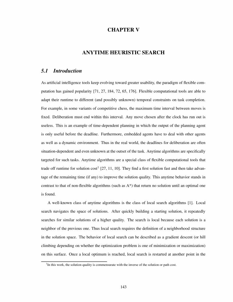
CHAPTER V
ANYTIME HEURISTIC SEARCH
5.1 Introduction
As artificial intelligence tools keep evolving toward greater usability, the paradigm of flexible com-
putation has gained popularity [71, 27, 184, 72, 65, 176]. Flexible computational tools are able to
adapt their runtime to different (and possibly unknown) temporal constraints on task completion.
For example, in some variants of competitive chess, the maximum time interval between moves is
fixed. Deliberation must end within this interval. Any move chosen after the clock has run out is
useless. This is an example of time-dependent planning in which the output of the planning agent
is only useful before the deadline. Furthermore, embedded agents have to deal with other agents
as well as a dynamic environment. Thus in the real world, the deadlines for deliberation are often
situation-dependent and even unknown at the outset of the task. Anytime algorithms are specifically
targeted for such tasks. Anytime algorithms are a special class of flexible computational tools that
trade off runtime for solution cost1 [27, 11, 10]. They find a first solution fast and then take advan-
tage of the remaining time (if any) to improve the solution quality. This anytime behavior stands in
contrast to that of non-flexible algorithms (such as A*) that return no solution until an optimal one
is found.
A well-known class of anytime algorithms is the class of local search algorithms [1]. Local
search navigates the space of solutions. After quickly building a starting solution, it repeatedly
searches for similar solutions of a higher quality. The search is local because each solution is a
neighbor of the previous one. Thus local search requires the definition of a neighborhood structure
in the solution space. The behavior of local search can be described as a gradient descent (or hill
climbing depending on whether the optimization problem is one of minimization or maximization)
on this surface. Once a local optimum is reached, local search is restarted at another point in the
1In this work, the solution quality is commensurate with the inverse of the solution or path cost.
143

solution space and the search proceeds iteratively until time runs out.
Although local search has been extremely popular both in the Operations Research (OR) and
Artificial Intelligence (AI) communities, it is not a common approach to the shortest-path problem.
One reason is that, unlike in typical optimization problems (such as the Traveling Salesperson Prob-
lem or TSP [111]), finding any solution to a shortest-path problem is hard since it requires search.
Second, the solution space contains structured elements (namely paths, not states like in standard
heuristic search). As a result, it is neither trivial to define a good neighborhood structure on paths
(namely one that induces a surface with few local optima) nor is it computationally efficient to
search it. Third, since building a starting solution (any solution, regardless of its quality) to the
shortest-path problem is computationally expensive, it is an open issue how to efficiently identify
additional restarting solutions to get the search agent out of local optima.
In this chapter, we propose a new anytime heuristic search algorithm called ABULB (for Any-
time BULB). It is a local search algorithm in the space of solution paths that addresses the three
aforementioned issues. In the previous chapter, we showed that BULB efficiently solves large prob-
lems. ABULB uses BULB to generate an initial solution. Section 5.2 describes the neighborhood
structure imposed on the solution space as well as a new local search algorithm (called ITSA*) that
searches the resulting surface. ITSA* has two variants depending on whether each iteration allows
for only one or multiple steps on the surface. Section 5.3 describes two ways of transforming BULB
into an anytime heuristic search algorithm that efficiently generates restarting solutions. The main
difference between these two variants of ABULB is whether the beam width varies during search.
Section 5.3.5 evaluates ABULB in two standard benchmark domains. Section 5.4 discusses related
and future work. Section 5.5 concludes by summarizing the contributions of this work.
5.2 ITSA*: Application of local search to the shortest-path problem
In this section, we first motivate our interest in local (or neighborhood) search.2 We then describe
a neighborhood structure on the space of solution paths. Finally, we introduce a new local opti-
mization algorithm (called ITSA*) that takes advantage of this neighborhood structure to greedily
explore the optimization surface.
2These methods are also called meta-heuristics (e.g., [166, 139]).
144

èRèRèRèRèRèRèRèRèRèRèRèRèRèRèRèRèèRèRèRèRèRèRèRèRèRèRèRèRèRèRèRèRèèRèRèRèRèRèRèRèRèRèRèRèRèRèRèRèRèèRèRèRèRèRèRèRèRèRèRèRèRèRèRèRèRèèRèRèRèRèRèRèRèRèRèRèRèRèRèRèRèRèèRèRèRèRèRèRèRèRèRèRèRèRèRèRèRèRèèRèRèRèRèRèRèRèRèRèRèRèRèRèRèRèRèèRèRèRèRèRèRèRèRèRèRèRèRèRèRèRèRèèRèRèRèRèRèRèRèRèRèRèRèRèRèRèRèRèèRèRèRèRèRèRèRèRèRèRèRèRèRèRèRèRèèRèRèRèRèRèRèRèRèRèRèRèRèRèRèRèRèèRèRèRèRèRèRèRèRèRèRèRèRèRèRèRèRèèRèRèRèRèRèRèRèRèRèRèRèRèRèRèRèRèèRèRèRèRèRèRèRèRèRèRèRèRèRèRèRèRèèRèRèRèRèRèRèRèRèRèRèRèRèRèRèRèRèèRèRèRèRèRèRèRèRèRèRèRèRèRèRèRèRèèRèRèRèRèRèRèRèRèRèRèRèRèRèRèRèRèèRèRèRèRèRèRèRèRèRèRèRèRèRèRèRèRèèRèRèRèRèRèRèRèRèRèRèRèRèRèRèRèRèèRèRèRèRèRèRèRèRèRèRèRèRèRèRèRèRè
éRéRéRéRéRéRéRéRéRéRéRéRéRéRéRéRééRéRéRéRéRéRéRéRéRéRéRéRéRéRéRéRééRéRéRéRéRéRéRéRéRéRéRéRéRéRéRéRééRéRéRéRéRéRéRéRéRéRéRéRéRéRéRéRééRéRéRéRéRéRéRéRéRéRéRéRéRéRéRéRééRéRéRéRéRéRéRéRéRéRéRéRéRéRéRéRééRéRéRéRéRéRéRéRéRéRéRéRéRéRéRéRééRéRéRéRéRéRéRéRéRéRéRéRéRéRéRéRééRéRéRéRéRéRéRéRéRéRéRéRéRéRéRéRééRéRéRéRéRéRéRéRéRéRéRéRéRéRéRéRééRéRéRéRéRéRéRéRéRéRéRéRéRéRéRéRééRéRéRéRéRéRéRéRéRéRéRéRéRéRéRéRééRéRéRéRéRéRéRéRéRéRéRéRéRéRéRéRééRéRéRéRéRéRéRéRéRéRéRéRéRéRéRéRééRéRéRéRéRéRéRéRéRéRéRéRéRéRéRéRééRéRéRéRéRéRéRéRéRéRéRéRéRéRéRéRééRéRéRéRéRéRéRéRéRéRéRéRéRéRéRéRééRéRéRéRéRéRéRéRéRéRéRéRéRéRéRéRééRéRéRéRéRéRéRéRéRéRéRéRéRéRéRéRééRéRéRéRéRéRéRéRéRéRéRéRéRéRéRéRé
êRêRêRêRêRêRêRêRêRêRêRêRêRêRêRêRêRêRêêRêRêRêRêRêRêRêRêRêRêRêRêRêRêRêRêRêRêêRêRêRêRêRêRêRêRêRêRêRêRêRêRêRêRêRêRêêRêRêRêRêRêRêRêRêRêRêRêRêRêRêRêRêRêRêêRêRêRêRêRêRêRêRêRêRêRêRêRêRêRêRêRêRêêRêRêRêRêRêRêRêRêRêRêRêRêRêRêRêRêRêRêêRêRêRêRêRêRêRêRêRêRêRêRêRêRêRêRêRêRêêRêRêRêRêRêRêRêRêRêRêRêRêRêRêRêRêRêRêêRêRêRêRêRêRêRêRêRêRêRêRêRêRêRêRêRêRêêRêRêRêRêRêRêRêRêRêRêRêRêRêRêRêRêRêRêêRêRêRêRêRêRêRêRêRêRêRêRêRêRêRêRêRêRêêRêRêRêRêRêRêRêRêRêRêRêRêRêRêRêRêRêRêêRêRêRêRêRêRêRêRêRêRêRêRêRêRêRêRêRêRêêRêRêRêRêRêRêRêRêRêRêRêRêRêRêRêRêRêRêêRêRêRêRêRêRêRêRêRêRêRêRêRêRêRêRêRêRêêRêRêRêRêRêRêRêRêRêRêRêRêRêRêRêRêRêRêêRêRêRêRêRêRêRêRêRêRêRêRêRêRêRêRêRêRêêRêRêRêRêRêRêRêRêRêRêRêRêRêRêRêRêRêRêêRêRêRêRêRêRêRêRêRêRêRêRêRêRêRêRêRêRêêRêRêRêRêRêRêRêRêRêRêRêRêRêRêRêRêRêRêêRêRêRêRêRêRêRêRêRêRêRêRêRêRêRêRêRêRê
ëRëRëRëRëRëRëRëRëRëRëRëRëRëRëRëRëRëëRëRëRëRëRëRëRëRëRëRëRëRëRëRëRëRëRëëRëRëRëRëRëRëRëRëRëRëRëRëRëRëRëRëRëëRëRëRëRëRëRëRëRëRëRëRëRëRëRëRëRëRëëRëRëRëRëRëRëRëRëRëRëRëRëRëRëRëRëRëëRëRëRëRëRëRëRëRëRëRëRëRëRëRëRëRëRëëRëRëRëRëRëRëRëRëRëRëRëRëRëRëRëRëRëëRëRëRëRëRëRëRëRëRëRëRëRëRëRëRëRëRëëRëRëRëRëRëRëRëRëRëRëRëRëRëRëRëRëRëëRëRëRëRëRëRëRëRëRëRëRëRëRëRëRëRëRëëRëRëRëRëRëRëRëRëRëRëRëRëRëRëRëRëRëëRëRëRëRëRëRëRëRëRëRëRëRëRëRëRëRëRëëRëRëRëRëRëRëRëRëRëRëRëRëRëRëRëRëRëëRëRëRëRëRëRëRëRëRëRëRëRëRëRëRëRëRëëRëRëRëRëRëRëRëRëRëRëRëRëRëRëRëRëRëëRëRëRëRëRëRëRëRëRëRëRëRëRëRëRëRëRëëRëRëRëRëRëRëRëRëRëRëRëRëRëRëRëRëRëëRëRëRëRëRëRëRëRëRëRëRëRëRëRëRëRëRëëRëRëRëRëRëRëRëRëRëRëRëRëRëRëRëRëRëëRëRëRëRëRëRëRëRëRëRëRëRëRëRëRëRëRëëRëRëRëRëRëRëRëRëRëRëRëRëRëRëRëRëRë
a) Admissible search b) Approximation search
S
G
S
G
Figure 55: Approximation algorithms explore the search space in a less regular way than admissiblealgorithms.
5.2.1 Motivation
Approximation algorithms sacrifice solution quality in order to reduce their runtime. Greedy algo-
rithms (such as WA*) rely heavily on the heuristic values by weighing them more than the g-values
in the computation of the f-values. Other approximation algorithms (such as beam search) rely even
more on the heuristic function by pruning nodes with high h-values. In both cases, the reliance on
the h-values gives the search a strong depth-first component. While depth-first search with perfect
information leads straight to the goal, it likely leads the search astray when combined with imper-
fect heuristic values. Nevertheless, both WA* and beam search are often able to use the heuristic
information to eventually reach the goal. These two characteristics of approximation algorithms
together imply that the solution path they find is often convoluted. They explore the search space
less systematically than admissible algorithms: Their search frontier grows in a jagged fashion (see
Figure 55b), as opposed to the regular exploration by admissible algorithms such as breadth-first
search and A* (see Figure 55a).
Because of the jagged shape of their search frontier, it is possible that approximation algorithms
miss shorter solutions that are actually close (in the space of solution paths) to the area of the search
space that they have explored (see Figure 55b). This possibility is confirmed empirically. For
145
Figure 56: Solutions found (unbroken line) and missed (dashed line) by WA* with �J� ��������in a gridworld problem.
146

example, Figure 56 depicts a concrete example of this situation for WA* in the gridworld domain,
whose two-dimensional structure enables a direct visualization of its search frontier. Obstacles are
black, expanded states are light gray, and the start and goal states are dark gray (with the goal on top).
The figure illustrates how the convoluted path found is longer (its cost is equal to fifty steps) than
but close to the optimal path (with a cost of thirty steps). Such patterns are also common for beam
search (and thus also BULB) as our empirical evaluation in two benchmark domains demonstrates
(see Section 5.2.4).
This behavior of approximation algorithms leads us to consider the following approach. In order
to avoid leaving some interspersed regions of the state space unexplored, we propose to focus the
search around a previously identified solution and to systematically explore its neighborhood. More
precisely, we envision a staged search. Prior to invoking the local search, we use an approximation
algorithm (such as BULB) to construct a sub-optimal solution. Then memory is purged except
for the solution path. A stage consists of the systematic exploration of the state space in expanding
concentric regions centered on the solution. When memory runs out, it is completely purged (though
the newly found best path is retained) and the stage ends. Successive stages are executed until the
quality of the evolving solution does not improve any more (or any other termination condition
is satisfied). When two successive stages return the same solution path, the search has reached a
(possibly local) minimum on the surface defined by the neighborhood relation and the cost function.
The next sub-section formally defines the neighborhood structure.
5.2.2 A neighborhood structure based on path proximity
Our overall approach to anytime heuristic search is to explore systematically the neighborhood of a
given solution path ì , find a minimum-cost path ì D in this neighborhood, then compute and search
the neighborhood centered around ì D , and repeat the process until a local minimum is found. The
size of each neighborhood is approximately equal to the maximum number of nodes that simulta-
neously fit in memory. Each neighborhood is built incrementally by including all nodes that can
be reached in one step from any node already in the neighborhood, starting with the initial neigh-
borhood containing the set of nodes in the current solution path. The analogy we use to describe
the process of building a neighborhood is that of iterative tunneling: If the solution path is seen
147

Iterations ofIterative Tunneling
Minimum−Cost PathFound After the
Third
First,
Second, and
G
S
S
G
States Newly
Third
First,
Second, and
Expanded During the
Iterations ofIterative Tunneling
Start State
Goal State
Other State
Figure 57: Iterative tunneling defines the neighborhood of a path.
as a narrow tunnel (dug into the search space) from start & to goal # , then each iteration enlarges
the diameter of the tunnel until there is no available space to heap any additional evacuated debris,
assuming memory is viewed as a container for debris/nodes (see Figure 57).
Formally, let %aíG(+*l, denote the graph defined by a finite set í of vertices (or nodes) and a finite
set * of directed edges . �F%0�61Q(4� 5<, between pairs of vertices � 1 , � 5À7Îí . & and # are two distinct
vertices called the start and goal vertices, respectively. Let î denote the set of paths from & to #in the graph. The elements of î are the states of our neighborhood search. First, we define the
distance metric ï � �ðí � í ñ òók/M�q9T between vertices in í that returns, for each pair of
vertices %0�21Q(4� 53, , the smallest number ï � %0�613(4� 53, of edges in any path from �61 to � 5 in the graph.
Second, we define the distance metric [ � ��î � îlñ ò between paths in î that returns, for each
pair of paths %6ì¶13( ìA5�, , the value ��¬�ôTõ+£+öHõ<M<�� I¡Aô4÷¨£+öK÷=ï � %0�213(4� 53,cT . [ � is commensurate with the
“distance” between two paths. Of course it holds that U ì�7�î : [ � %6ìp( ì ,^� m . Third, given a path
ì 7mî and V�7�ò , let ø-%6ìp(4V¨,À� M�ì�D67mîùs [ � %6ìp( ìEDj,E�KV4T . Then, the neighborhood ú %6ìÎ( ã�, of
solution path ì given the available memory ã is the set ø-%6ìp(4V¨, such that ø-%6ìÎ(4V¨, fits into memory
and U�V'D�7nò : V'DÃ|ÂV implies ø-%6ìÎ(4VtDI, does not fit into memory.
148
5.2.3 The ITSA* algorithm
Having defined the neighborhood of a path, we now turn to the issue of how to search it. The task
is to find the shortest path from start to goal through states in the neighborhood. We need to answer
two questions, namely how to identify such states and how to find the shortest path completely
contained in the region of the state space that they occupy. Once the states in the neighborhood are
identified, there is a simple answer to the second question, namely to use (a simple variant of) A*.
The identification of the states in the neighborhood of a path ì is performed in a way similar
to the way a ball is inflated, namely from the center out. The neighborhood is to ì as the ball is to
its center. As the interior of the ball is the union of concentric spheres of increasing radii around
the center (starting with a radius of zero for the center point itself), the states in the neighborhood
distribute themselves in layers of increasing distances (i.e., number of edges) from ì (starting with
a distance of 0, namely the states in ì itself). In computational terms, a simple extension of breadth-
first search suffices to identify the states layer by layer.
There is therefore a simple two-stage process for finding the shortest-path in the neighborhood
of ì , namely 1) to generate and store in memory the neighborhood states using breadth-first search
applied in parallel to all states in ì (this search stops when memory is full), and 2) to use A* to find
the shortest path through stored states only. However, this approach has two drawbacks. First, it
performs two full explorations of the neighborhood (once with breadth-first search, once with A*)
before returning a solution. Second, because A* delays the expansion of states with large f-values,
some states in the neighborhood may never be visited by A* and therefore need not be stored in
memory. Unfortunately, these states cannot be identified during the first, breadth-first search stage.
They occupy memory that might be used by A* for one (or more) extra layer(s).
To address both problems, we propose to interleave the building of the neighborhood with its
search by A* in order to take advantage of the pruning power of f-values during construction and
thus make the neighborhood as large as possible. We call the resulting algorithm ITSA* (for Iter-
ative Tunneling Search with A*, and pronounced It’s-a-star). ITSA* iteratively performs modified
A* searches from the start to the goal. ITSA* assigns each generated state an iteration (or layer)
number. This number corresponds to the distance of the state from (a state in) the path ì . Once
149

Table 22: Performance of one-step ITSA* on paths found by BULB in the 48-Puzzle (with 6 millionnodes in memory)
BULB BULB + one-step ITSA*time cost time (seconds) cost
(seconds) value increase over BULB value decrease over BULBabsolute relative absolute relative
5 0.1 11,737 5.7 5.6 5,600% 3,140 8,597 73%10 0.9 36,282 6.7 5.8 644% 3,233 33,049 91%100 6.1 14,354 12.2 6.1 100% 2,052 12,302 86%
1,000 7.3 1,409 12.8 5.5 75% 746 663 47%10,000 21.7 440 27.7 6.0 28% 428 12 3%
assigned (at the time of the state’s generation), this number never changes. Before the call to ITSA*,
all states in ì are stored in memory with a layer number equal to zero. Then A* is run repeatedly
with an increasing iteration number (starting at one) until memory runs out. At the beginning of
each iteration, the OPEN list is initialized to the start state. A* proceeds as usual except that 1)
it only inserts into the OPEN list states whose layer number is less than the iteration number, and
2) each newly generated state is assigned a layer number equal to one plus that of its parent in the
search tree. Each iteration ends when A* is about to expand the goal state (except possibly for the
last iteration, which ends when the memory is full).
Instead of performing two full explorations of a pre-existing neighborhood (built with breadth-
first search, as discussed above), ITSA* performs several A* searches over a region of the search
space that grows around ì in a layered fashion. Only the last iteration of ITSA* is a complete A*
search over the entire neighborhood. Furthermore, ITSA* outputs a (potentially better) path at the
end of each A* iteration. This anytime behavior of ITSA* is discussed in Section 5.3.1. In the next
sub-section, we evaluate the performance of ITSA* as a local optimization procedure.
5.2.4 Empirical evaluation of ITSA*
We evaluate the performance of ITSA* as a local optimization algorithm in two standard benchmark
domains, namely the 48-Puzzle and the Rubik’s Cube. We run ITSA* on solution paths found by
BULB in 50 random instances for each domain. We report the solution quality output by ITSA*
and its runtime, which we compare to that of BULB (see Tables 22 through 25).
First, we discuss the performance of one-step ITSA* (see Tables 22 & 23), where ITSA* is
150
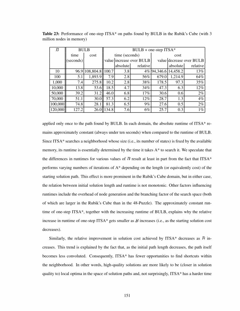
Table 23: Performance of one-step ITSA* on paths found by BULB in the Rubik’s Cube (with 3million nodes in memory)
BULB BULB + one-step ITSA*time cost time (seconds) cost
(seconds) value increase over BULB value decrease over BULBabsolute relative absolute relative
10 96.9 108,804.8 100.7 3.8 4% 94,346.6 14,458.2 13%100 5.1 1,893.9 7.9 2.8 56% 679.0 1,214.9 64%
1,000 7.4 275.8 10.2 2.8 38% 178.5 97.3 35%10,000 13.8 53.6 18.5 4.7 34% 47.3 6.3 12%50,000 39.2 31.2 46.0 6.8 17% 30.6 0.6 2%70,000 51.1 30.0 57.3 6.2 12% 28.7 1.3 4%100,000 74.8 28.1 81.3 6.5 9% 27.6 0.5 2%120,000 127.2 26.0 134.8 7.6 6% 25.7 0.3 1%
applied only once to the path found by BULB. In each domain, the absolute runtime of ITSA* re-
mains approximately constant (always under ten seconds) when compared to the runtime of BULB.
Since ITSA* searches a neighborhood whose size (i.e., its number of states) is fixed by the available
memory, its runtime is essentially determined by the time it takes A* to search it. We speculate that
the differences in runtimes for various values of result at least in part from the fact that ITSA*
performs varying numbers of iterations of A* depending on the length (or equivalently cost) of the
starting solution path. This effect is more prominent in the Rubik’s Cube domain, but in either case,
the relation between initial solution length and runtime is not monotonic. Other factors influencing
runtimes include the overhead of node generation and the branching factor of the search space (both
of which are larger in the Rubik’s Cube than in the 48-Puzzle). The approximately constant run-
time of one-step ITSA*, together with the increasing runtime of BULB, explains why the relative
increase in runtime of one-step ITSA* gets smaller as increases (i.e., as the starting solution cost
decreases).
Similarly, the relative improvement in solution cost achieved by ITSA* decreases as in-
creases. This trend is explained by the fact that, as the initial path length decreases, the path itself
becomes less convoluted. Consequently, ITSA* has fewer opportunities to find shortcuts within
the neighborhood. In other words, high-quality solutions are more likely to be (closer in solution
quality to) local optima in the space of solution paths and, not surprisingly, ITSA* has a harder time
151
Table 24: Performance of multi-step ITSA* on paths found by BULB in the 48-Puzzle (with 6million nodes in memory)
BULB BULB + multi-step ITSA*time cost time (seconds) cost
(seconds) value increase over BULB value decrease over BULBabsolute relative absolute relative
5 0.1 11,737 50.3 50.2 50,200% 2,562 9,175 78%10 0.9 36,282 53.0 52.1 5,789% 1,808 34,474 95%100 6.1 14,354 55.2 49.1 805% 1,159 13,195 92%
1,000 7.3 1,409 36.7 29.4 409% 674 735 52%10,000 21.7 440 42.4 20.7 95% 426 14 3%
Table 25: Performance of multi-step ITSA* on paths found by BULB in the Rubik’s Cube (with 3million nodes in memory)
BULB BULB + multi-step ITSA*time cost time (seconds) cost
(seconds) value increase over BULB value decrease over BULBabsolute relative absolute relative
10 96.9 108,804.8 111.3 14.4 15% 94,346.6 14,458.2 13%100 5.1 1,893.9 23.2 18.1 356% 578.5 1,315.4 69%
1,000 7.4 275.8 22.1 14.7 199% 156.8 119.0 43%10,000 13.8 53.6 28.1 14.3 104% 45.3 8.3 15%50,000 39.2 31.2 49.8 10.6 27% 30.4 0.8 3%70,000 51.1 30.0 62.4 11.3 22% 28.7 1.3 4%100,000 74.8 28.1 86.1 11.3 15% 27.5 0.6 2%120,000 127.2 26.0 137.4 10.2 8% 25.7 0.3 1%
improving on higher quality solutions (ceiling effect).3
Second, we discuss the performance of multi-step ITSA* (see Tables 24 & 25), where we apply
ITSA* iteratively, first to the path found by BULB, and then repeatedly to the best path found
during the previous execution of ITSA*. Multi-step ITSA* can stop as soon as ITSA* returns its
starting path which is then a local minimum in the space of paths. For efficiency reasons, instead of
checking the path itself, we only check its length. So we stop multi-step ITSA* when the solution
cost it returns is equal to that of its starting solution.
3The case Ù,�Ä�w� stands out in Table 23. With such a narrow beam width, BULB reaches deeply into the search spaceand the cost of the solution is over 100,000. Given that 1) the branching factor in the Rubik’s Cube is approximately equalto 13 and 2) the available memory can store up to 3 million nodes, ITSA* can only perform one complete iteration ofA* before memory runs out. The neighborhood only extends as far as layer one and the relative improvement in solutionquality is thus low. Similarly, because BULB is so slow in this case, ITSA*’s relative increase in runtime is small.
152
In both domains, the absolute runtime of multi-step ITSA* tends to decrease as increases. As
the initial path cost decreases, it is harder for local search to improve it and ITSA* is called fewer
times before it reaches a local minimum. In addition, since the runtime of BULB increases with
, the relative increase in runtime of multi-step ITSA* decreases as increases. Finally, both the
absolute and relative improvements in solution quality decrease as increases because again, better
solutions are harder to improve on.
5.3 ABULB: Anytime BULB
In this section, we discuss three ways of transforming BULB into an anytime algorithm. First, the
solution output by BULB is improved by an anytime local search algorithm such as ITSA*. Second,
BULB is kept running after it finds a goal. Third, BULB is restarted with a different value of upon finding a goal. We present these three variants in the first three sub-sections, respectively.
Then, we discuss how to combine the use of ITSA* with the last two variants. Finally, we evaluate
all resulting variants in our two benchmark domains.
5.3.1 BULB + ITSA*: Local optimization of BULB’s solutions
ITSA*, as a local search algorithm, is also an anytime algorithm. First, one-step ITSA* returns
solutions of non-increasing cost at the end of each iteration of A*. Second, multi-step ITSA*
repeatedly applies ITSA* to solution paths with lower and lower costs until a local minimum is
reached.
While ITSA* is a general purpose anytime algorithm for local path optimization, we propose
to apply it to the solution output by BULB. More specifically, once BULB terminates with a path
ì to the goal, all states not in ì are purged from memory and multi-step ITSA* is started with all
states in ì assigned to the zero s � layer and OPEN initialized to the start state (see Section 5.2.3).
The only parameter of this anytime algorithm is the value of the beam width used by BULB. We
choose a low value of so that the first solution is quickly found.
Since this chapter focuses on anytime algorithms (such as ITSA*), we need to be able to repre-
sent the performance of an anytime algorithm. The standard representation is a performance profile,
that is the expected solution quality output by the algorithm as a function of time. We follow the
153

time
qual
ity
a) Data points obtained for one instancetime
qual
ity
b) Corresponding stair function
0
20
40
60
80
100
0 5 10 15 20
Red
uctio
n in
Sol
utio
n C
ost R
elat
ive
to In
itial
Sol
utio
n (p
erce
nt)
Time in Seconds
c) Data points obtained for fifty instances
0
20
40
60
80
100
0 5 10 15 20
Red
uctio
n in
Sol
utio
n C
ost R
elat
ive
to In
itial
Sol
utio
n (p
erce
nt)
Time in Seconds
d) Corresponding stair functions
0
20
40
60
80
100
0 5 10 15 20
Red
uctio
n in
Sol
utio
n C
ost R
elat
ive
to In
itial
Sol
utio
n (p
erce
nt)
Time in Seconds
e) Corresponding average performance profile
Figure 58: Building a performance profile
154

0
20
40
60
80
100
0 20 40 60 80 100
Red
uctio
n in
Sol
utio
n C
ost R
elat
ive
to In
itial
Sol
utio
n (p
erce
nt)
Time in Seconds
local optimization with ITSA*completion of multi-step ITSA*completion of one-step ITSA*
BULB
Figure 59: Performance of ITSA* on solutions produced by BULB in the 48-Puzzle (with 6 millionnodes and B=5)
standard procedure to obtain the performance profile [183]. First, we compute the quality û as the
improvement in solution quality of each new solution path ì D relative to the original solution path
ì (in our case, the one found by BULB). Thus, û��ýü Õ 3�5�¦Iö § ` ü Õ 365'¦Iö ¢ §ü Õ 3�5t¦þö § . The performance profile plots
û as a function of ÿ , the time taken to produce ì D from ì . Thus, ÿG� @C>A¡�F6B � <a%6ì D , Á.@C>A¡�F6B � <�%6ì , .4Figure 58a shows such data points corresponding to one instance. Note that solutions are found
at irregular time intervals. Since the solution quality does not change between two successive data
points, we fill in equally spaced points to yield a staircase function (see Figure 58b). Figures 58c & d
contain the real and “filled in” data (respectively) for the complete set of fifty test instances. Finally,
the performance profile is obtained by fitting a curve through the resulting cloud of points (for each
time slice, we compute the average quality improvement of all points in the slice). We call this
curve the performance profile.
The performance profile in Figure 58e is actually that of ITSA* when applied to solutions found
by BULB in the 48-Puzzle. We reproduce it in Figure 59. In addition, the figure shows the average
completion time (and the corresponding quality improvement achieved) for one-step and multi-step
ITSA*. The reason these points do not sit squarely on the curve is explained in Figure 60 with
4Note that defining the runtime as the time elapsed since the first solution is produced abstracts away the variance inthe runtimes of BULB over the set of instances.
155
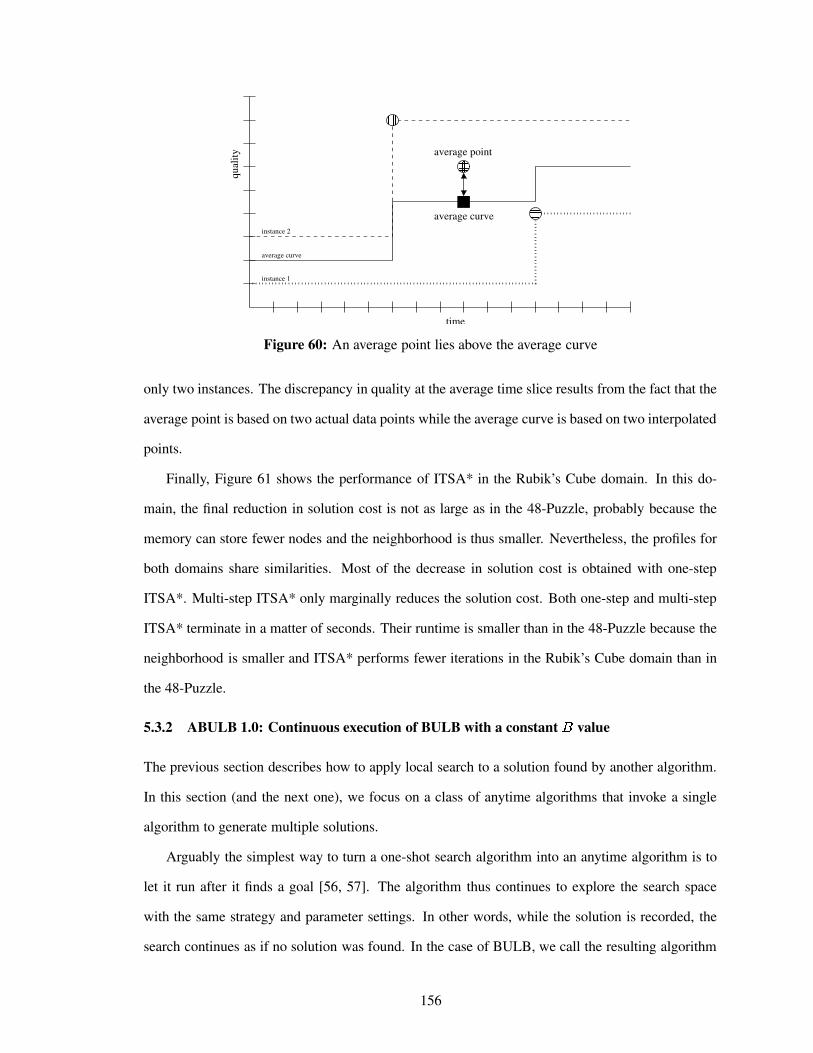
average curve
average curve
average point������������
qual
ity
time
instance 1
instance 2
������������������
��������������
Figure 60: An average point lies above the average curve
only two instances. The discrepancy in quality at the average time slice results from the fact that the
average point is based on two actual data points while the average curve is based on two interpolated
points.
Finally, Figure 61 shows the performance of ITSA* in the Rubik’s Cube domain. In this do-
main, the final reduction in solution cost is not as large as in the 48-Puzzle, probably because the
memory can store fewer nodes and the neighborhood is thus smaller. Nevertheless, the profiles for
both domains share similarities. Most of the decrease in solution cost is obtained with one-step
ITSA*. Multi-step ITSA* only marginally reduces the solution cost. Both one-step and multi-step
ITSA* terminate in a matter of seconds. Their runtime is smaller than in the 48-Puzzle because the
neighborhood is smaller and ITSA* performs fewer iterations in the Rubik’s Cube domain than in
the 48-Puzzle.
5.3.2 ABULB 1.0: Continuous execution of BULB with a constant value
The previous section describes how to apply local search to a solution found by another algorithm.
In this section (and the next one), we focus on a class of anytime algorithms that invoke a single
algorithm to generate multiple solutions.
Arguably the simplest way to turn a one-shot search algorithm into an anytime algorithm is to
let it run after it finds a goal [56, 57]. The algorithm thus continues to explore the search space
with the same strategy and parameter settings. In other words, while the solution is recorded, the
search continues as if no solution was found. In the case of BULB, we call the resulting algorithm
156

0
20
40
60
80
100
0 5 10 15 20
Red
uctio
n in
Sol
utio
n C
ost R
elat
ive
to In
itial
Sol
utio
n (p
erce
nt)
Time in Seconds
local optimization with ITSA*completion of multi-step ITSA*completion of one-step ITSA*
BULB
Figure 61: Performance of ITSA* on solutions produced by BULB in the Rubik’s Cube domain(with 1 million nodes and B=70)
Anytime BULB or ABULB for short. Since the next section describes a different approach also based
on BULB, we call this version ABULB 1.0.
ABULB 1.0 is a complete and admissible algorithm since it searches the whole search tree
rooted at the start state down to a depth whose value depends on the parameter settings. Recall that
the maximum depth reached by BULB is approximately equal to ã��� , where ã is the maximum
number of nodes that can fit simultaneously in memory and is the beam width. This upper bound
on the search depth follows from the fact that BULB stores at most nodes at each level of its
search tree. Therefore, ABULB 1.0 is complete and admissible whenever the depth of a shallowest
goal state is less than or equal to this bound. In addition, ABULB 1.0 is an anytime algorithm since
it finds a sequence of solutions and can at any time return the best solution found so far. Because it
maintains a dynamic upper bound (to be described shortly) on the optimal solution cost, ABULB 1.0
is guaranteed to return solutions of monotonically increasing quality.
Figure 62 depicts the behavior of ABULB 1.0. It behaves exactly like BULB until the first goal
( #-1 in the figure) is found. Then, two modifications are enforced. First, the search continues as
long as time remains to find better and better solutions ( # 5 , then # » in the figure). Second, the
depth of successive BULB searches is bounded from above by decreasing values. Indeed, it is easy
157

upper bound
B
depth 1
depth 2
depth 3
start
at level 1discrepancy
first
discrepancyfirst
at level 2
based on depth 2
upper bound based on depth 1
initial upper boundG
2
1
G
G3
Figure 62: Behavior of ABULB 1.0
to maintain a dynamic upper bound on the solution cost (or depth).5 This upper bound is initialized
to the maximum searchable depth (namely �� ) until the first goal is found. Then, every time
a goal is found, the upper bound is reduced based on the latest goal’s cost (or depth). During the
search, all candidate nodes whose depth is larger than the upper bound are pruned (i.e., they are not
generated). As the search proceeds, the upper bound decreases and the pruning power increases,
until an optimal goal is found.
The only input parameter of ABULB 1.0 is , the beam width. Its value is set at the time the
algorithm is called and is never modified. Since the first solution should be found quickly, we set to a small (domain-dependent and empirically determined) value.
5.3.3 ABULB 2.0: Restart of BULB with varying values
In this section, we consider another instance in the class of anytime approaches that use a single
algorithm to generate multiple solutions. In this instance, a single algorithm is called with different
parameter settings. We propose to make successive calls to BULB with different values of . Recall
5Or equivalently, a lower bound on the solution quality.
158

depth 2
depth 3
B1
initial upper bounddepth 1
start
B
B
2
3
upper bound based on depth 2
upper bound based on depth 1
G1
G3
G2
Figure 63: Behavior of ABULB 2.0
that larger values of tend to generate solutions of higher quality, since BULB behaves more and
more like breadth-first search. Therefore, ABULB 2.0 first calls BULB with a small value of to
quickly find a first solution and then repeatedly calls BULB with increasing values of to improve
the solution quality until time runs out.
Figure 63 depicts the behavior of ABULB 2.0. It behaves exactly like BULB until the first goal
( #-1 in the figure) is found. Then, like in ABULB 1.0, a new upper bound is computed based on
the cost of the best solution found so far. However, unlike ABULB 1.0, a new value of is also
computed. One important weakness of ABULB 1.0 is that it does not use all the available memory.
As time goes by, the upper bound decreases. Thus, the search gets more and more shallow. Since
its beam width remains constant (equal to ), ABULB 1.0 uses less and less memory. ABULB 2.0
addresses this issue by increasing the value of in such a way that the product of and the upper
bound on the search depth remains equal to ã (the maximum number of nodes storable in memory).
Every time a goal is found (say # ] in the figure), is updated to a value that is slightly larger thandepth ] .
Like for BULB and ABULB 1.0, the behavior of ABULB 2.0 depends on the initial value of .
A low value typically returns the first solution quickly. In addition, the schedule of updates also
159
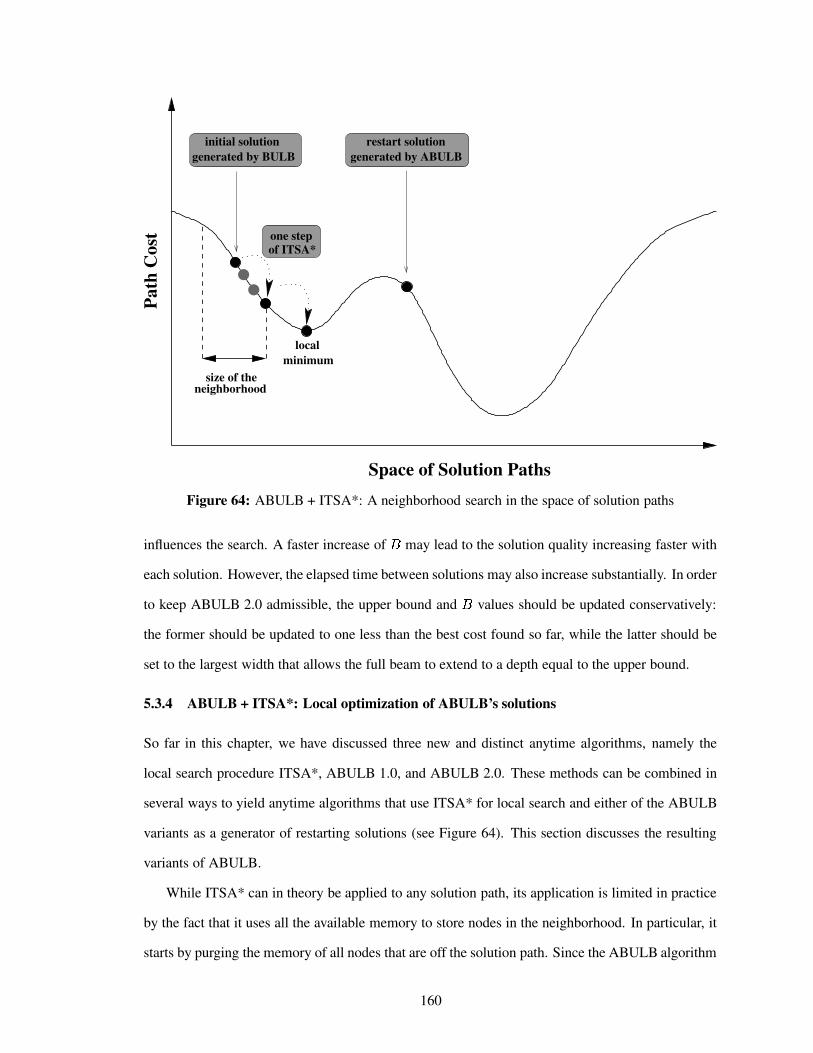
generated by ABULB
one step
generated by BULBrestart solution
of ITSA*
initial solution
Space of Solution Paths
Path
Cos
t
neighborhoodsize of the
localminimum
Figure 64: ABULB + ITSA*: A neighborhood search in the space of solution paths
influences the search. A faster increase of may lead to the solution quality increasing faster with
each solution. However, the elapsed time between solutions may also increase substantially. In order
to keep ABULB 2.0 admissible, the upper bound and values should be updated conservatively:
the former should be updated to one less than the best cost found so far, while the latter should be
set to the largest width that allows the full beam to extend to a depth equal to the upper bound.
5.3.4 ABULB + ITSA*: Local optimization of ABULB’s solutions
So far in this chapter, we have discussed three new and distinct anytime algorithms, namely the
local search procedure ITSA*, ABULB 1.0, and ABULB 2.0. These methods can be combined in
several ways to yield anytime algorithms that use ITSA* for local search and either of the ABULB
variants as a generator of restarting solutions (see Figure 64). This section discusses the resulting
variants of ABULB.
While ITSA* can in theory be applied to any solution path, its application is limited in practice
by the fact that it uses all the available memory to store nodes in the neighborhood. In particular, it
starts by purging the memory of all nodes that are off the solution path. Since the ABULB algorithm
160
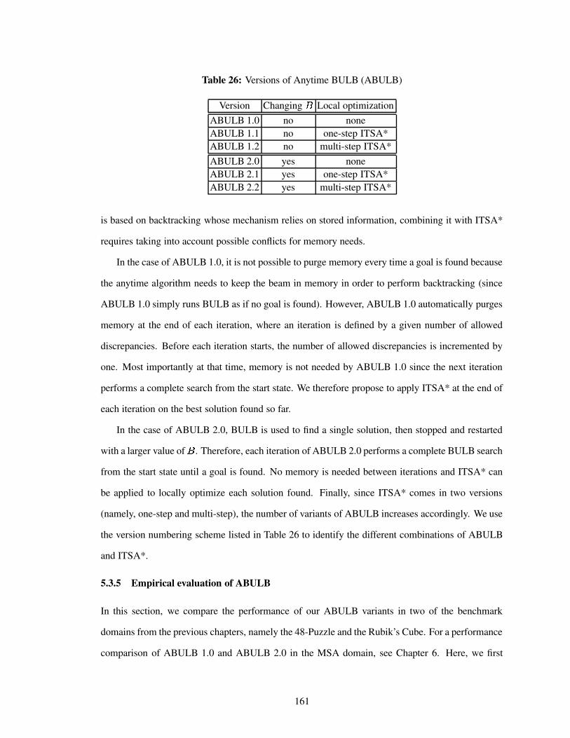
Table 26: Versions of Anytime BULB (ABULB)
Version Changing Local optimizationABULB 1.0 no noneABULB 1.1 no one-step ITSA*ABULB 1.2 no multi-step ITSA*ABULB 2.0 yes noneABULB 2.1 yes one-step ITSA*ABULB 2.2 yes multi-step ITSA*
is based on backtracking whose mechanism relies on stored information, combining it with ITSA*
requires taking into account possible conflicts for memory needs.
In the case of ABULB 1.0, it is not possible to purge memory every time a goal is found because
the anytime algorithm needs to keep the beam in memory in order to perform backtracking (since
ABULB 1.0 simply runs BULB as if no goal is found). However, ABULB 1.0 automatically purges
memory at the end of each iteration, where an iteration is defined by a given number of allowed
discrepancies. Before each iteration starts, the number of allowed discrepancies is incremented by
one. Most importantly at that time, memory is not needed by ABULB 1.0 since the next iteration
performs a complete search from the start state. We therefore propose to apply ITSA* at the end of
each iteration on the best solution found so far.
In the case of ABULB 2.0, BULB is used to find a single solution, then stopped and restarted
with a larger value of . Therefore, each iteration of ABULB 2.0 performs a complete BULB search
from the start state until a goal is found. No memory is needed between iterations and ITSA* can
be applied to locally optimize each solution found. Finally, since ITSA* comes in two versions
(namely, one-step and multi-step), the number of variants of ABULB increases accordingly. We use
the version numbering scheme listed in Table 26 to identify the different combinations of ABULB
and ITSA*.
5.3.5 Empirical evaluation of ABULB
In this section, we compare the performance of our ABULB variants in two of the benchmark
domains from the previous chapters, namely the 48-Puzzle and the Rubik’s Cube. For a performance
comparison of ABULB 1.0 and ABULB 2.0 in the MSA domain, see Chapter 6. Here, we first
161
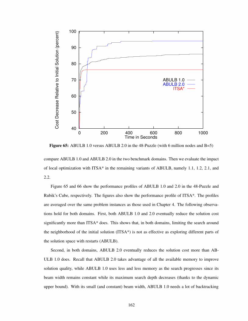
40
50
60
70
80
90
100
0 200 400 600 800 1000
Cos
t Dec
reas
e R
elat
ive
to In
itial
Sol
utio
n (p
erce
nt)
Time in Seconds
ABULB 1.0ABULB 2.0
ITSA*
Figure 65: ABULB 1.0 versus ABULB 2.0 in the 48-Puzzle (with 6 million nodes and B=5)
compare ABULB 1.0 and ABULB 2.0 in the two benchmark domains. Then we evaluate the impact
of local optimization with ITSA* in the remaining variants of ABULB, namely 1.1, 1.2, 2.1, and
2.2.
Figure 65 and 66 show the performance profiles of ABULB 1.0 and 2.0 in the 48-Puzzle and
Rubik’s Cube, respectively. The figures also show the performance profile of ITSA*. The profiles
are averaged over the same problem instances as those used in Chapter 4. The following observa-
tions hold for both domains. First, both ABULB 1.0 and 2.0 eventually reduce the solution cost
significantly more than ITSA* does. This shows that, in both domains, limiting the search around
the neighborhood of the initial solution (ITSA*) is not as effective as exploring different parts of
the solution space with restarts (ABULB).
Second, in both domains, ABULB 2.0 eventually reduces the solution cost more than AB-
ULB 1.0 does. Recall that ABULB 2.0 takes advantage of all the available memory to improve
solution quality, while ABULB 1.0 uses less and less memory as the search progresses since its
beam width remains constant while its maximum search depth decreases (thanks to the dynamic
upper bound). With its small (and constant) beam width, ABULB 1.0 needs a lot of backtracking
162

0
20
40
60
80
100
0 200 400 600 800 1000
Cos
t Dec
reas
e R
elat
ive
to In
itial
Sol
utio
n (p
erce
nt)
Time in Seconds
ABULB 1.0ABULB 2.0
ITSA*
Figure 66: ABULB 1.0 versus ABULB 2.0 in the Rubik’s Cube domain (with 1 million nodes andB=70)
and thus is slower to reduce the solution cost. Its performance profile takes longer to level off than
that of ABULB 2.0. However, in the 48-Puzzle only, ABULB 1.0 is better than ABULB 2.0 during
the first 60 seconds or so.
We now consider the variants of ABULB that use ITSA* for local optimization. Fig-
ures 67 and 68 show that, in the 48-Puzzle, local optimization with ITSA* improves the perfor-
mance of ABULB 1 and ABULB 2.0, respectively. First, in both figures, plain ABULB (i.e., without
ITSA*) is the algorithm that eventually exhibits the smallest decrease in solution cost. Therefore,
combining ITSA* with ABULB, is always better in the long run in this domain. Second, in both
figures, the combination of multi-step ITSA* with ABULB (i.e., ABULB � .2) yields the largest
decrease in solution cost in the long run. Overall, ABULB 2.2 is the best algorithm in this domain
for long-term performance. In contrast, one-step ITSA* yields the largest decrease in solution cost
at the outset (again in both figures). Overall, ABULB 2.1 is the best algorithm in this domain for
short-term performance.
Figures 69 and 70 show a different picture in the Rubik’s Cube domain. In this domain, neither
163
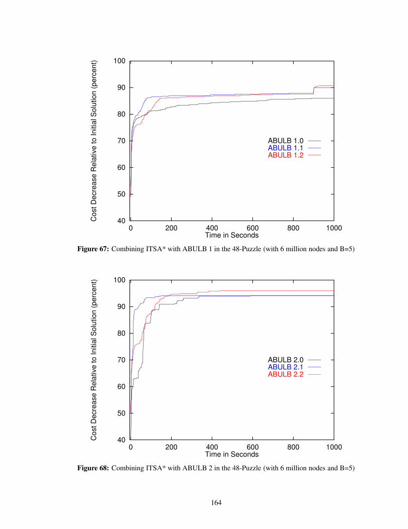
40
50
60
70
80
90
100
0 200 400 600 800 1000
Cos
t Dec
reas
e R
elat
ive
to In
itial
Sol
utio
n (p
erce
nt)
Time in Seconds
ABULB 1.0ABULB 1.1ABULB 1.2
Figure 67: Combining ITSA* with ABULB 1 in the 48-Puzzle (with 6 million nodes and B=5)
40
50
60
70
80
90
100
0 200 400 600 800 1000
Cos
t Dec
reas
e R
elat
ive
to In
itial
Sol
utio
n (p
erce
nt)
Time in Seconds
ABULB 2.0ABULB 2.1ABULB 2.2
Figure 68: Combining ITSA* with ABULB 2 in the 48-Puzzle (with 6 million nodes and B=5)
164
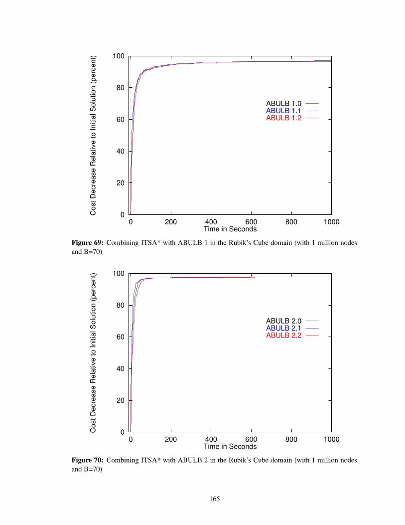
0
20
40
60
80
100
0 200 400 600 800 1000
Cos
t Dec
reas
e R
elat
ive
to In
itial
Sol
utio
n (p
erce
nt)
Time in Seconds
ABULB 1.0ABULB 1.1ABULB 1.2
Figure 69: Combining ITSA* with ABULB 1 in the Rubik’s Cube domain (with 1 million nodesand B=70)
0
20
40
60
80
100
0 200 400 600 800 1000
Cos
t Dec
reas
e R
elat
ive
to In
itial
Sol
utio
n (p
erce
nt)
Time in Seconds
ABULB 2.0ABULB 2.1ABULB 2.2
Figure 70: Combining ITSA* with ABULB 2 in the Rubik’s Cube domain (with 1 million nodesand B=70)
165

one-step nor multi-step ITSA* significantly improves the performance profile when combined with
ABULB. The decrease in solution cost obtained by letting BULB run (in ABULB 1.0) or by restart-
ing it (in ABULB 2.0) outweighs the decrease in solution cost obtained with ITSA*. The latter is
(relatively) small because, as pointed out before, the large branching factor and the tight memory
constraints allow for only a small number of A* iterations within ITSA*.
5.4 Related work
In this section, we describe related work in both anytime heuristic search and local search.
5.4.1 Anytime heuristic search
In time-dependent tasks, the quality of a solution depends not only on its intrinsic characteristics,
but also on how fast it is produced. In AI, the notion of time-dependency was first coined in the
context of planning [27]. Since one of the main constraints in time-dependent planning is time, it
makes sense to try and make optimal use of this resource. However, when considering the trade-off
between planning time and plan quality, approximation and admissible algorithms appear to be two
discrete points at each end of a spectrum. On the one hand, approximation algorithms are as fast
as possible with or without guarantee on solution cost (that is, by how much it exceeds the shortest
path). On the other hand, admissible algorithms guarantee optimality of the solution at the expense
of (potentially) exponential time of execution. In other words, admissible algorithms consider time
as secondary compared to the solution quality, while approximation algorithms do the reverse. In
both cases, the trade-off is fixed.
Anytime algorithms were introduced to provide greater flexibility when trading off time and
solution quality [71, 27, 11]. The usefulness of anytime algorithms is obvious when compared to the
two following extremes. First, the solution produced by an admissible algorithm can be completely
useless if it comes too late. Second, the solution produced by an approximation algorithm can come
too early, in the sense that it is produced before it is actually needed as input to a subsequent problem
solving stage whose start time has not come yet. This wasted time interval could have been used
to improve the approximate solution. Anytime algorithms are designed to provide such flexibility
when dealing with uncertain time constraints.
166

There exist only a few anytime heuristic search algorithms to date. The most relevant ones are
variants of WA* (Weighted A*).
Anytime A* (ATA*) [56, 57, 178] is a best-first search algorithm that maintains for each node
both an A*-like f-value and a weighted f-value. The only difference between weighted best-first
search and Anytime A* is that it does not stop after a solution is found. Instead, the search continues
and the cost of the lowest-cost solution found so far is used as an upper bound on the cost of
a minimum-cost solution. Such an upper bound serves to prune nodes in the OPEN list whose
(unweighted) f-value is larger than or equal to the upper bound. Since this bound decreases over
time, the set of nodes that can be pruned increases and Anytime A* eventually finds a minimum-cost
solution. ATA* is thus to WA* as ABULB 1.0 is to BULB.
ARA* [114, 115] is another variant of WA* that is more closely related to ABULB 2.0 since
it repeatedly calls WA* with decreasing weights on the h-values (whereas ABULB 2.0 repeatedly
calls BULB with increasing values). One difference between ARA* and ABULB 2.0 is that
ARA* reuses some of the search effort of the previous WA* search to speed up the current iteration.
Combining ideas in incremental search with ABULB is an interesting direction for future research.
However, the main limitation of these variants of WA* is that they do not control their memory
consumption (other than by increasing the weight on the h-values). Therefore, both algorithms can
only solve problems that WA* can solve. In contrast, we have shown in this dissertation that BULB
and ABULB, as memory-bounded algorithms, scale up to much larger domains.
Finally, all other anytime heuristic search algorithms known to us are variants of depth-first
search. For example, DFBnB (depth-first branch-and-bound) is a variant of branch-and-bound
search [112, 110]. It is a depth-first search that uses h-values to order the successors for expan-
sion and upper bounds to prune some of them. Another example is Complete Anytime Beam search
(CABS) [173]. CABS repeatedly calls a variant of depth-first search with a pruning rule that is
progressively weakened at each iteration. As the pruning rule weakens, fewer and fewer nodes are
pruned. In the worst case, no pruning occurs and thus CABS is complete.
The main weakness of these depth-first search algorithms from our perspective is that they do
not scale well to general graph-search problems (such as our benchmark domains and the multiple
sequence alignment problem described in Chapter 6) since they cannot detect transpositions and thus
167
tend to suffer from an exponential overhead in node re-generations. Nevertheless, such methods are
well suited to problems with a high density of solutions or a finite search tree [135]. DFBnB is very
efficient on the Traveling Salesperson Problem [111], for instance [174, 175].
5.4.2 Local search
Local or neighborhood search methods (also called (meta-)heuristics) have been applied by the OR
community to a large number of combinatorial problems [166, 139]. However, virtually all these
problems share the characteristic that a sub-optimal solution can be found easily (without search).
In the Traveling Salesperson Problem (TSP) [111] for example, a feasible solution is a permutation
of an explicit set of cities, while in the boolean satisfiability problem (SAT) [148], a feasible solution
is an assignment of truth-values to an explicit set of boolean variables. In contrast, in the shortest-
path problem, a solution (path) is a sequence of states (or equivalently state-action pairs). Since
the states are too numerous to list explicitly, only a small list of action schemata (or operators) are
provided and finding any path requires search.
Neighborhood search is sometimes called iterative-improvement search [144, 1], since solution
quality is improved by iteratively jumping from one path to another one in the subset of the solution
space defined as the neighborhood. This general paradigm leaves open the question of how to select
the next solution path within the neighborhood. ITSA* follows a best-improvement [1] or steepest-
descent [130] strategy, since it uses a variant of A* to select the solution of highest quality within the
neighborhood. Alternatively, a first-improvement strategy would stop searching the neighborhood
when any solution is found with higher quality than the current solution.
5.5 Conclusion
In this chapter, we have presented a new family of anytime heuristic search algorithms generically
called ABULB (Anytime BULB). ABULB is a local (or neighborhood) search algorithm in the
space of solution paths. ABULB uses BULB to find both an initial solution and restarting solutions.
ABULB can also take advantage of ITSA* for local path optimization.
ITSA* (Iterative Tunneling Search with A*, pronounced It’s a star) is a new local path opti-
mization algorithm. ITSA* imposes a neighborhood structure on the space of solution paths based
168

on our definition of distance between paths. ITSA* interleaves the construction and the searching
of the neighborhood using breadth-first and A* search, respectively. Each iteration returns a path
of smaller cost. ITSA* is thus an anytime algorithm in its own right. ITSA* performs gradient
descent on the surface whose connectivity and elevation result from the neighborhood structure and
the solution cost, respectively. Each time ITSA* reaches a (possibly local) minimum on the surface,
ABULB generates a new restarting solution of higher quality.
Our empirical study has shown that, while ITSA* reduces the solution cost over time when used
as an anytime algorithm in the 48-Puzzle and the Rubik’s Cube domain, an even larger reduction
in solution cost is achieved by letting BULB 1) run after it finds a solution or 2) by restarting it
with a larger, automatically computed beam width. Furthermore, combining ITSA* with either
anytime modification of BULB yields an even larger reduction in solution cost in the 48-Puzzle.
In the Rubik’s Cube however, no significant improvement (or degradation) was observed in the
performance profile of ABULB when adding ITSA*.
This research has produced the following contributions:
k We have introduced a new local path optimization (namely, ITSA*) based on a search strategy
called iterative tunneling.
k We have described and empirically evaluated different ways of transforming BULB into an
anytime algorithm, both with and without dynamic beam widths.
k To the best of our knowledge, our way of combining ABULB with ITSA* is the first success-
ful application of local (or neighborhood) search to the shortest path problem.
Possible avenues for future work include:
k studying the effect of neighborhood size on the performance of ITSA*; for example, can its
runtime be decreased by reducing the neighborhood size to a portion of the available memory
with an acceptable loss in solution quality? In this case, how best to take advantage of the
freed memory?,
k studying the effect of initial solution quality on the quality of local optima found by ITSA*;
169

for example, what happens if the quality of restarting solutions does not increase monotoni-
cally as is currently the case for ABULB?,
k studying how the trade-off between runtime and solution quality in ABULB (i.e., the slope
of the performance profile) is affected by the schedule of value updates; for example, can
smaller increments in values lead to steeper profiles?, and
k studying domain-dependent properties that influence the performance of our neighborhood
search; for example, how does the graph connectivity, say the number of small loops, affect
the local optimization performed by ITSA*?
170

CHAPTER VI
THE MULTIPLE SEQUENCE ALIGNMENT PROBLEM
In this chapter, we use the multiple sequence alignment (MSA) problem as an additional benchmark
domain for ABULB. We explain how the MSA problem reduces to the shortest-path problem. We
describe how to apply ABULB to the MSA problem and show empirically that ABULB scales up
to larger MSA problems than an existing anytime heuristic search algorithm based on WA*.
6.1 Introduction
The primary structure of biological sequences is essentially a linear string of characters over a
small alphabet. The primary structure of a nucleic acid such as DNA, for example, is a sequence
of characters from the 4-element alphabet M A,C,G,T T , while proteins are sequences of characters
from the 20-element set of amino acids (also called residues). Over the past decade or so, the
number of available sequences has grown exponentially, as powerful new sequencing technology
has emerged. Whenever a new sequence is identified, biologists are interested in determining both
its function (for a gene or an enzyme, for example) and its 3-dimensional configuration (for proteins
in general). While the most reliable approach remains the empirical one, it is quite time-consuming.
This explains the need for, and the great progress of, computational approaches.
One way to infer the function (or 3-dimensional structure) from a linear sequence is to compare
the new sequence to available sequences with known functions. For example, the function of a newly
discovered protein may be inferred by determining its membership in a known family of proteins.
Similarly, the function of a gene (DNA sequence) can be inferred by comparison to similar genes
with known functions. However, to assess the similarity between a new sequence and one or more
known sequences first requires the alignment of these sequences. This explains why the multiple
sequence alignment problem is one of the most important challenges in computational biology.
171

Figure 71: Three pairwise alignments (taken from [33])
6.2 Sequence alignment
To align sequences means to write them one under the other, one letter per column. All the letters in
a column are said to be aligned. Figure 71(a) depicts the alignment of the same region of two human
protein sequences referred to as HBA-HUMAN and HBB-HUMAN in the SWISS-PROT database.1
The protein sequences occupy the first and third lines in the figure. The middle line is not part of
the alignment per se. It is added in order to make it easy to visually identify columns that contain a
“good” alignment. Since two sequences are being aligned, each column of the alignment contains
two letters. When the two letters in a column are identical, the letter is repeated in the middle line
to highlight the perfect match. When the two letters are different but represent similar residues, a
plus sign is inserted in the middle line to highlight a close but imperfect match (the similarity of
residues, or equivalently the closeness of a match, is measured by a scoring function to be described
in the next section). Finally, a blank in the middle line highlights a column where two dissimilar
residues are aligned. Large numbers of letters and plus signs in the middle line, combined with a
small number of blanks, indicate that the human alpha globin (HBA-HUMAN) is very similar to
the human beta globin (HBB-HUMAN).
In Figure 71(b), the same region of the human alpha globin is aligned with another sequence
(called LGB2-LUPLU). In this case, the proportion of perfect and close matches is smaller than
1The SWISS-PROT database is accessible at http://kr.expasy.org/sprot/.
172

in the alignment of Figure 71(a) but still large enough to indicate a possible relationship between
the two globins. Indeed, this alignment is meaningful to biologists since these two globins are
evolutionarily related and share structural and functional properties. Notice that this alignment is
longer than the one in Figure 71(a), that is, it is made up of a larger number of columns. This is
because, in the process of aligning the sequences, five gaps were inserted into the first sequence.
Each gap is represented by a dash. In columns containing a dash, the residue in the second sequence
is not aligned with any residue in the first sequence. Assuming that the two globins are evolutionarily
related, a gap indicates that the residue in the same column was either deleted in the first sequence
or inserted into the second sequence during evolution. In contrast, a plus sign in a column suggests
that both residues are evolutionarily related through mutations. Either one evolved from the other,
or both evolved from a common ancestor. Finally, a perfect match in a column suggests that the
corresponding residue remained unchanged through evolution.
6.3 Evaluating alignments
The alignment in Figure 71(c) has approximately the same length and total number of letters and
plus signs in the middle line as the alignment in Figure 71(b). Unfortunately, this alignment is
spurious because the F11G11.2 protein is neither functionally nor structurally similar to the human
alpha globin. Simply counting the number of (close) matches in the alignment is not sufficient to
discriminate between meaningful and spurious alignments. A more sophisticated evaluation method
is needed.
Biological sequences evolve via the selection of random mutations. We consider three types of
mutations. A substitution replaces one residue with another, while an insertion or a deletion adds
or removes a residue (or a group of residues). Determining the biological significance of an align-
ment requires a lot of expert knowledge of phylogenetic constraints on mutations, the properties of
various groups of contiguous elements, the influence of higher-order structure, etc. Automating the
alignment process requires the design of numerical formulas to capture these constraints. Statistical
analyses are used to generate a likelihood ratio for each pair of residues. Each ratio estimates the
odds of the pair appearing in the same column due to a phylogenetic relationship as opposed to a
random occurrence. The set of ratios for all possible pairs of residues makes up a score matrix or
173
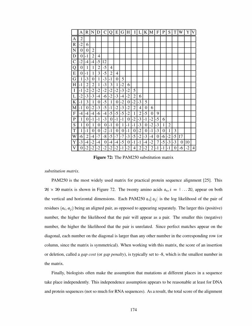
A R N D C Q E G H I L K M F P S T W Y VA 2R -2 6N 0 0 2D 0 -1 2 4C -2 -4 -4 -5 12Q 0 1 1 2 -5 4E 0 -1 1 3 -5 2 4G 1 -3 0 1 -3 -1 0 5H -1 2 2 1 -3 3 1 -2 6I -1 -2 -2 -2 -2 -2 -2 -3 -2 5L -2 -3 -3 -4 -6 -2 -3 -4 -2 2 6K -1 3 1 0 -5 1 0 -2 0 -2 -3 5M -1 0 -2 -3 -5 -1 -2 -3 -2 2 4 0 6F -4 -4 -4 -6 -4 -5 -5 -5 -2 1 2 -5 0 9P 1 0 -1 -1 -3 0 -1 -1 0 -2 -3 -1 -2 -5 6S 1 0 1 0 0 -1 0 1 -1 -1 -3 0 -2 -3 1 2T 1 -1 0 0 -2 -1 0 0 -1 0 -2 0 -1 -3 0 1 3W -6 2 -4 -7 -8 -5 -7 -7 -3 -5 -2 -3 -4 0 -6 -2 -5 17Y -3 -4 -2 -4 0 -4 -4 -5 0 -1 -1 -4 -2 7 -5 -3 -3 0 10V 0 -2 -2 -2 -2 -2 -2 -1 -2 4 2 -2 2 -1 -1 -1 0 -6 -2 4
Figure 72: The PAM250 substitution matrix
substitution matrix.
PAM250 is the most widely used matrix for practical protein sequence alignment [25]. This
!Ym � !Ym matrix is shown in Figure 72. The twenty amino acids � ] (4Vl� �2PQPQP?!Ym�( appear on both
the vertical and horizontal dimensions. Each PAM250 W ��]0\³W �� Q\ is the log likelihood of the pair of
residues %�� ] (�� , being an aligned pair, as opposed to appearing separately. The larger this (positive)
number, the higher the likelihood that the pair will appear as a pair. The smaller this (negative)
number, the higher the likelihood that the pair is unrelated. Since perfect matches appear on the
diagonal, each number on the diagonal is larger than any other number in the corresponding row (or
column, since the matrix is symmetrical). When working with this matrix, the score of an insertion
or deletion, called a gap cost (or gap penalty), is typically set to -8, which is the smallest number in
the matrix.
Finally, biologists often make the assumption that mutations at different places in a sequence
take place independently. This independence assumption appears to be reasonable at least for DNA
and protein sequences (not so much for RNA sequences). As a result, the total score of the alignment
174

of two protein or DNA sequences is simply the sum of the pairwise scores over all the columns in
the alignment. Similarly, a so-called linear gap cost (i.e., -8) is added for each column where
a gap appears, including adjacent columns.2 With this scoring scheme, the alignments in Fig-
ures 71(b) and 71(c) have scores of 1 and -5, respectively, thereby correctly discriminating between
the case of two related sequences (b) and the case of two unrelated sequences (c). Indeed, pos-
itive scores indicate that the sequences are more likely in meaningful alignments than in random
alignments, while negative scores indicate just the opposite. However, in general, no such scoring
scheme is guaranteed to reliably discriminate between meaningful and spurious alignments in all
cases. An optimal alignment is only as good as the scoring scheme used to evaluate it.
6.4 Pairwise sequence alignment
From now on, we take for granted the scoring scheme described in the previous section and turn our
attention to algorithms used for finding an alignment of two sequences that has a maximum score
according to this scheme.
A standard way of building a complete alignment of two sequences is to use optimal alignments
of smaller sub-sequences. This is the underlying principle for a dynamic programming algorithm
called the Needleman-Wunsch algorithm [125, 55]. We explain the behavior of this algorithm using
the example in Figure 73(a). Let ��%0Vc(��a, denote the score of the optimal alignment of the two
sequences made up of the first V letters of the first sequence and the first � letters of the second
sequence, respectively. Therefore, �¸%©m�(+m�,��}m since the corresponding alignment is empty, and
��%0Ç (4Ça, is the score of the optimal alignment of the two complete sequences. In general, the value
of �¸%0V+(��a, can be computed using the values of �¸%0VÎÁC�Y(���ÁC�<, , �¸%0VÎÁC�Y(��a, and �¸%0V+(��JÁ��<, .For example, suppose we want to compute ��%w�Y(3�<, , the score of the optimal alignment of the first
letter in each sequence (i.e., ‘D’). There are only three ways to build such an alignment using
smaller alignments. First, the empty alignment (with zero column) can be extended to a one-column
alignment that aligns both first letters with no gap (see Figure 73b). The score of this alignment is
��%©m�(+m�, � PAM250 W �¸\³W ��\Ã�"m � Ç-�9Ç . Second, the one-column alignment with score ��%w�Y(+m�, can
2In some cases, an affine gap score is used, in which long contiguous insertions or deletions are penalized less thanthe gap cost times the number of consecutive gaps.
175

Sequence 1: DQLF Sequence 2: DNVQ
a) Two sequences to be aligned
M empty T�� DD
b) No gap inserted
D–� D –
– D
c) Gap in the first sequence
–D� – D
D –
d) Gap in the second sequence
C(1,1)=4C(0,1)=−8 −8
−8
10
1
0 C(0,0)=0 C(1,0)=−8
+PAM250[D][D]
e) �¸%w�Y(3�<,6� max( ��%©m�(+m�, � PAM250 W ��\³W �¸\ , �¸%©m�(3�<,2Árz , �¸%w�Y(+m�,)Árz )= max( m � Ç , Á$zªÁ�z , Á$zÀÁrz ) = 4
−8
j
C(i−1,j−1)
C(i,j)C(i−1,j)
C(i,j−1)
−8
ii−1
j−1
+PAM250[.][.]
f) ��%0V+(���,6� max( �¸%0V·Áo�Y(�� Áo�<, � PAM250 W � 1] \³W � 5 \ , ��%0V ÁÐ�Y(��a,2Á�z , ��%0V+(�� Áo�<,)Á�z )Figure 73: One step in the alignment of two sequences
176

10 1 n0
0
1
n2
a) Row by row
10 1 n0
0
1
n2
b) Column by column
Figure 74: The Needleman-Wunsch dynamic programming algorithm
be extended to a two-column alignment that aligns the ‘D’ in the second sequence with a gap (see
Figure 73c). The score of this alignment is �¸%w�Y(+m�, � %¨Á$z{,-�/Á§z-Áoz���Á �3È , where Á$z is the
gap cost. Third, the one-column alignment with score ��%©m�(3�<, can be extended into a two-column
alignment that aligns the ‘D’ in the first sequence with a gap (see Figure 73d). The score of this
alignment is �¸%©m�(3�<, � %¨Á$z{,^�CÁ$zªÁ�z���Á �3È . Finally, the optimal alignment of the first letter in
each sequence is the one with the largest score, namely the one-column alignment that matches ‘D’
with ‘D’, since Ç � max( Ç (QÁ �3È�(QÁ �3È{, .In general, ��%0V+(���, is calculated as the maximum of three numbers: 1) the sum of �¸%0V�Á��Y(��¶Á��<,
and the PAM250 score of aligning � 1] (i.e., the V s � letter in the first sequence) and � 5 (i.e., the � s � letter
in the second sequence); 2) the sum of ��%0V�Á8�Y(��a, and the gap cost; and 3) the sum of ��%0Vc(��·Á8�<, and
the gap cost. The score function �¸%0V+(��a, is stored as a two-dimensional matrix, with the number V of
letters in the first sequence serving as index in the horizontal dimension and the number � of letters
in the second sequence serving as index in the vertical dimension. Figure 73e depicts the calculation
of ��%w�Y(3�<, using this two-dimensional representation. Figure 73f depicts the general case of �¸%0V+(��a, .The Needleman-Wunsch dynamic programming algorithm fills up the two-dimensional matrix
� either row by row or column by column, as depicted in Figure 74. The score of the optimal
alignment of the two original sequences is the last number calculated, that is, the number in the
bottom-right cell of the matrix. The result of applying the Needleman-Wunsch algorithm to the
example in Figure 73a is shown in Figure 75. Note that each number in the first column (the first
row) is a multiple of the gap cost since each cell in this column (row) corresponds to inserting one
177
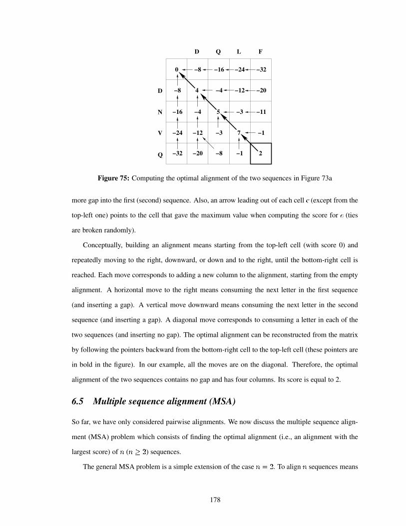
Q
−16
−4
5
−3
−8
D
−8
4
−4
−12
−20
L
−24
−12
−3
7
−1
F
−32
−20
−11
−1
2
0
−8
−16
−24
−32
D
N
V
Q
Figure 75: Computing the optimal alignment of the two sequences in Figure 73a
more gap into the first (second) sequence. Also, an arrow leading out of each cell = (except from the
top-left one) points to the cell that gave the maximum value when computing the score for = (ties
are broken randomly).
Conceptually, building an alignment means starting from the top-left cell (with score 0) and
repeatedly moving to the right, downward, or down and to the right, until the bottom-right cell is
reached. Each move corresponds to adding a new column to the alignment, starting from the empty
alignment. A horizontal move to the right means consuming the next letter in the first sequence
(and inserting a gap). A vertical move downward means consuming the next letter in the second
sequence (and inserting a gap). A diagonal move corresponds to consuming a letter in each of the
two sequences (and inserting no gap). The optimal alignment can be reconstructed from the matrix
by following the pointers backward from the bottom-right cell to the top-left cell (these pointers are
in bold in the figure). In our example, all the moves are on the diagonal. Therefore, the optimal
alignment of the two sequences contains no gap and has four columns. Its score is equal to 2.
6.5 Multiple sequence alignment (MSA)
So far, we have only considered pairwise alignments. We now discuss the multiple sequence align-
ment (MSA) problem which consists of finding the optimal alignment (i.e., an alignment with the
largest score) of � ( � ~Ð! ) sequences.
The general MSA problem is a simple extension of the case ���"! . To align � sequences means
178

start
D
DQDNDN
DQDD
−4
−1
8 8
88
D
Figure 76: Search tree for the 2-dimensional MSA problem in Figure 73a
to write them down, one under the other, so that each letter belongs to a column. All the letters in
a column are said to be aligned. Gaps can be inserted at any position in any of the sequences, as
long as no column of the alignment is completely filled with gaps. In other words, each column
must consume one letter in at least one sequence. For example, Figure 78b depicts one possible
alignment of the three sequences listed in Figure 78a.
The method for computing the score of an alignment is generalized as follows. The total score
remains the sum of the scores of all the columns in the alignment. In other words, we continue to
make the assumption that random mutations at different positions in a sequence are independent
from one another. However, the score of each column is now computed as the sum of the scores
of all the pairs of letters in the column. The gap is treated as any other letter, except that any pair
containing at least one gap has a score equal to the gap cost, that is, score(–, any letter) = score(any
letter, –) = score(–, –) = Á$z .The Needleman-Wunsch dynamic programming algorithm readily extends to the MSA problem.
In the general case, the score matrix is an � -dimensional matrix. It is built in row-major or column-
major order. The score of the alignment is computed last, in the corner cell opposite the start cell.
Pointers are maintained in each cell in order to reconstruct the alignment backward from the corner
cell.
179

goal
N
V
Q
DNVQDQLF
DQL−FD−NVQ
D Q L Fstart
D
Figure 77: State space for the 2-dimensional MSA problem in Figure 73a
b) One possible alignment
D N V Q
DQLFDNVQQGL
−N−
−
−V
QQQ
−−G
L−L
F−−
DD−
LQ
D
F
L
G
Q
c) State space and path corresponding to the alignment
goal
start
a) Three sequences to be aligned
Figure 78: A 3-dimensional MSA problem
180

6.6 The MSA problem as a shortest-path problem
It is well-known that the MSA problem of finding a maximum-score alignment of � sequences
is equivalent to the problem of finding a shortest path in an � -dimensional lattice [18]. In this
formulation, each node in the graph corresponds to an alignment of some prefix of each sequence.
The start node corresponds to the alignment of all empty prefixes. An edge corresponds to adding
one column to the right of an existing partial alignment, and the cost of the edge is equal to the score
of the added column multiplied by negative one. The goal node corresponds to the alignment of all
complete sequences. In this formulation, finding a maximum-score alignment reduces to finding a
minimum-cost path from the start node to the goal node. The state space for an � -dimensional MSA
problem is an � -dimensional grid. We illustrate this reduction using cases with ���"! and ���"Ì .Let us reconsider the two sequences in Figure 73a. Assume that in the first step, we decide
(out of three choices) to align the first letter ‘D’ of the first sequence with the first letter ‘D’ of the
second sequence. The resulting alignment (or node) contains only one column. The cost of the
edge leading from the start node to this node is -4. At the next step, there are again three choices.
First, the letter ‘Q’ in the first sequence may be aligned with the letter ‘N’ in the second sequence;
second, a gap may be inserted into the first sequence; third, a gap may be inserted into the second
sequence. Figure 76 depicts this (partial) search tree. The graph corresponding to the search space
for this problem is the 2-dimensional grid shown in Figure 77. Its 25 nodes are the intersection
points of the vertical and horizontal lines defining the grid. The start and goal nodes are at opposite
corners of the grid. The edges in this graph are the horizontal and vertical line segments connecting
pairs of adjacent nodes, as well as the diagonal line segments (not shown in the figure) connecting
the top-left corner of each grid cell to its bottom-right corner. The edges are directed from left to
right, or from top to bottom, or both (for diagonal moves). Each alignment of the two complete
sequences corresponds to a path in this graph from the start node to the goal node. Figure 77
shows two examples of such path-alignment pairs. In general, there is a one-to-one correspondence
between the set of all possible alignments of the two sequences and the set of all paths from the start
node to the goal node in this grid. Since the cost of each edge is equal to the negative value of the
score of the corresponding letter pair (diagonal edge) or the gap cost (horizontal or vertical edge), a
181

minimum-cost path determines an optimal alignment.
This one-to-one correspondence between paths and alignments extends to MSA problems with
three sequences. In this case, the search space is a 3-dimensional grid or cube. Figure 78c shows
the search space for the problem of aligning the three sequences in Figure 78a, as well as the path
corresponding to the alignment in Figure 78b. In general, the problem of aligning � sequences can
be reduced to the problem of finding a shortest path in an � -dimensional hypercube in which each
dimension corresponds to one of the sequences to be aligned.
6.7 Solving the MSA problem with search algorithms
Since each MSA problem reduces to a shortest-path problem in a grid, we can use search algorithms
to solve it. The defining characteristic of a search algorithm is the order in which it expands nodes.
In this context, the Needleman-Wunsch dynamic programming algorithm can be construed as a
search algorithm that expands nodes in a fixed order, namely either in row-major or column-major
order (see Figure 74). This algorithm takes advantage of the domain-specific structure of the state
space when ordering node expansions. But any node ordering strategy may be used.
For example, Figure 79a depicts a breadth-first search strategy for solving the MSA problem
in the 2-dimensional case. In contrast to the Needleman-Wunsch algorithm, breadth-first search
expands nodes layer by layer, where each layer is perpendicular to the main diagonal of the grid.
The main drawback of both the Needleman-Wunsch algorithm and breadth-first search is that they
generate the complete search space before finding an optimal alignment. Since both algorithms
store every node they generate, and since there are on the order of � ô nodes in an � -dimensional
MSA problem of length- � sequences, these algorithms run out of memory before finding a solution
to large problems.
For this reason, heuristic search approaches are being used in the AI community to solve the
MSA problem. Figures 79b and 79c depict the behavior of beam search and A* search in the 2-
dimensional MSA problem. Both heuristic search algorithms are able to find an alignment without
generating the whole state space. While A* is guaranteed to find an optimal alignment (when using
an admissible heuristic function), beam search is not. However, beam search can explicitly control
its memory consumption (via its beam width parameter ) and scales up to larger problems than
182

a) Breadth-first search b) Beam search
c) A* search
Figure 79: Solving the MSA problem with search algorithms
183
A*, as we will show shortly. Both beam search and the A* algorithm need a heuristic function
to guide the search. In the next section, we describe a powerful heuristic function for the MSA
problem.
6.7.1 An admissible heuristic function for the MSA problem
The cost of an alignment is the sum of the costs of each column in the alignment. The cost of each
column is in turn the sum of the costs of each pair of letters (or gaps) in the column. Therefore,
the cost of an alignment is also equal to the sum of the costs of the alignments of all the pairs of
sequences in the alignment. For example, the cost of an alignment of three (four) sequences is the
sum of the costs of three (six) pairwise alignments, since there are three (six) ways of pairing three
(four) sequences.
Since the cost of an � -dimensional alignment is the sum of the costs of all pairwise align-
ments, and since the cost of any pairwise alignment is by definition larger than or equal to the cost
of the optimal pairwise alignment, the sum of the costs of the optimal pairwise alignments never
overestimates the cost of the optimal � -dimensional alignment. This observation is the basis for
a well-known admissible heuristic function for the MSA problem [158], which we now describe
using the Ì -dimensional MSA problem shown in Figure 78a.
The first step in solving this MSA problem is to compute the optimal cost of each pairwise
alignment of the three sequences, as shown in Figure 80a. The h-value of the start node for this
problem is equal to 3 (see Figure 80b), which is the sum of the costs in the bottom right cell in
each of the three matrices in Figure 80a. The start node has seven successor nodes, since there are
seven possible first columns in a three-way alignment, depending on whether the first letter of each
sequence is part of the column or not. In order to compute the h-value of these successor nodes,
we need to know the costs of the optimal pairwise alignments of the remaining suffixes of the three
sequences, that is, the sequences minus the letter consumed in the first column, if any. These costs
can be read off the pre-computed matrices shown in Figure 80a. Notice that these matrices compute
the costs of aligning the reversed sequences, not the original sequences. We illustrate the h-value
computation using the middle successor node in Figure 80b, which turns out to have the smallest
h-value.
184
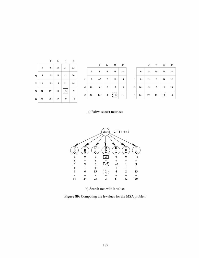
16
10
3
11
19
Q
24
12
11
2
9
Q
V
N
D
0
8
16
24
32
D
32
20
14
9
−2
F
8
5
9
17
25
L
L 8
16
24
D
32
18
9
1
F
8
−2
6
14
L
16
2
2
8
Q
24
10
3
−2Q
G
0
2
8
16
24Q
G
L
8
Q
2
16
V
6
24
N
14
D
32
22
4
9 3 6 13
17 11
0
a) Pairwise cost matrices
D
start
2+3+6=11
+
+
=11
9
−2
4
+
+
=
−2
9
13
20
2+
+
=
−2
2
2
D D DD
DQ Q QDD
Q
−2 + 1 + 4 = 3
+
+6=
+3+
=
+
+
=
9
9
24
9
25
13
9
1
2
12
b) Search tree with h-values
Figure 80: Computing the h-values for the MSA problem
185

Like for every node in this problem, the h-value is the sum of three costs. First, we consider the
pairwise alignment of the first two sequences. Since the first letter of each sequence (i.e., ‘D’) is
consumed in the first column of the alignment, we estimate the cost of aligning the suffixes of the
sequences, starting with the letters ‘Q’ and ‘N’, respectively. The cost of an optimal alignment of
these sub-sequences is stored in the marked cell of the leftmost matrix in Figure 80a. Second, we
consider the pairwise alignment of the first and third sequences. Since a gap is inserted in the third
sequence, its first letter is not consumed. The cost of an optimal alignment of the first sub-sequence
and the complete third sequence is stored in the marked cell of the middle matrix in Figure 80a.
Third, we consider the pairwise alignment of the second and third sequences. Since a gap is inserted
in the third sequence, its first letter is not consumed. The cost of an optimal alignment of the second
sub-sequence and the complete third sequence is stored in the marked cell of the rightmost matrix in
Figure 80a. Finally, the h-value of the middle successor of the start node is equal to ! � %¨Á�!{, � !�� ! .A similar h-value calculation is used for all generated nodes in the search tree. When a goal node is
reached, all letters in each sequence have been consumed. Therefore, the remaining sub-sequences
are empty and the values looked up in the three matrices are all equal to zero (the value in the top
left cell). The h-value of the goal node is thus zero, as must be the case for an admissible heuristic
function.
The heuristic we have just described is a memory-based heuristic [23, 181]. Unlike (memo-
ryless) heuristic functions, such as the Manhattan distance used in the�
-Puzzle that compute the
h-value from scratch for each state description, memory-based heuristics use lookup tables stored
in memory. The pairwise-cost heuristic function for the MSA problem must store in memory all the
pairwise cost matrices. However, the time and space requirements for this heuristic are negligible
when solving large alignment problems. It is the most popular heuristic function used by the AI
search community [74, 124, 178, 67] and we use it in our experiments. More informed heuristics
exist that store � -dimensional alignments ( ��~KÌ ) instead of pairwise alignments [120]. However,
they are much more memory intensive and cannot be stored in full. The mechanisms needed to
combine their partial storage with on-demand computation make them much harder to use.
186

6.7.2 Solving the MSA problem with existing variants of A*
Over the past decade, several variants of the A* algorithm have been used to solve the MSA problem
[74, 75, 124, 113, 109, 172, 181, 182]. Since the pairwise-cost heuristic is admissible, its use in the
A* algorithm guarantees that the alignment found is optimal. However, the main drawback of
A* is that it runs out of memory on large alignments because it stores in memory all the nodes it
generates. Much of the research on the application of heuristic search to the MSA problem has
focused on reducing the memory consumption of A*, by decreasing the size of either its OPEN list
or its CLOSED list. A third approach is based on linear-space search. We describe these approaches
in turn.
One characteristic of the MSA problem is its large branching factor. In fact, its branching factor
is exponential in the number � of sequences to be aligned: since there are ! ô -1 distinct ways of
inserting between 0 and ��ÁÐ� gaps into each � -dimensional column of the alignment, the number
of successors of a node in the MSA problem is ɸ%�! ô , . For this reason, the nodes in the OPEN list
(i.e., the set of nodes that have been generated but not yet expanded) use up a significant percentage
of the memory needed by A*. To address this problem, [172] proposed a variant of A* with partial
expansion in which only some of the newly-generated successor nodes are added into the OPEN
list, namely those with the best estimated cost. The advantage of this approach is that the goal node
may be found without having to store many of the nodes in the OPEN list with high f-values.
The second set of approaches aim at reducing the size of the CLOSED list, that is, the set of
nodes that have already been expanded. In A*, the CLOSED list has two main functions. First, it
serves to construct the solution path (that is, the optimal alignment in the case of MSA) by following
pointers backwards from the goal node to the start node. Second, it serves to avoid re-expanding
nodes that can be reached from the start node along several paths. Because of the lattice structure of
the search space for the MSA problem, there are many paths going through each node. If multiple
paths are not detected, each node in the MSA problem may be expanded an exponential number
of times. [102, 109] proposed a divide-and-conquer approach that does not store the CLOSED
list at all. Instead, once the goal node is found, the solution path is constructed by breaking the
current MSA problem into two sub-problems and solving them recursively. Node re-expansions are
187

prevented by maintaining, for each open node, pointers to the incoming edges that have already been
visited, as well as by storing additional “dummy” open nodes. In contrast, instead of discarding
the whole CLOSED list, [179] proposed to store a fraction of it. This sparse representation of
the CLOSED list has several advantages. First, the resulting algorithm behaves like A* when the
latter has enough memory to complete the search. Second, the path-constructing phase is more
efficient than the recursive approach. Third, the sparse memory-approach can easily be combined
with approaches that reduce the size of the OPEN list.
Yet a different approach for reducing the memory consumption of A* is to use linear-space
algorithms, such as IDA* [96]. Such algorithms use a depth-first search strategy and therefore only
store in memory the path currently being explored. When the goal is found, the solution path is
easily reconstructed (again backwards) using the calling stack. Unfortunately, because they do not
store generated nodes, they are extremely slow on lattice-like search spaces. [124] applied a new
variant of IDA* called SNC (for Stochastic Node Caching) to the MSA problem. In order to prevent
some of the node re-expansions of IDA*, SNC stores a fraction of the generated nodes, namely
those that are most likely to be visited often. The main goal of SNC is thus to speed up IDA* by
reducing the time spent on re-expansions.
Because of the exponential size and the lattice structure of the MSA search space (and despite
the existence of the well-informed pairwise-cost heuristic function), existing variants of A* can only
find optimal alignments of � real proteins (of average length equal to approximately 500 amino
acids) for values of � that are smaller than 10 on typical current machine configurations. This
limitation of optimal heuristic-search-based MSA solvers is one motivation for sacrificing solution
optimality in order to scale up to larger problems. Another motivation is the fact that the scoring
scheme for the MSA problem is only an approximation of the complex knowledge used by biologists
to estimate the phylogenetic significance of an alignment. Since optimality is measured using an
imperfect scale, it may be more practical to find good enough or even near-optimal solutions to
larger MSA problems than to insist on finding strictly optimal alignments. We follow this practical
approach for the experiments reported in this chapter, in which we apply our anytime approximation
algorithms to the MSA problem. In the next section, we compare the performance of ABULB to a
variant of Weighted A* (or WA* [132, 131]) called Anytime A* (ATA* [178]). ATA*, like WA*,
188

puts more weight on the h-value than on the g-value when computing the f-value of each node. WA*
scales up to larger problems than A* at the expense of solution quality. ATA* simply extends WA*
in an anytime fashion by continuing its execution even after a goal is found.
6.8 Solving the MSA problem with ABULB
In this section, we motivate and describe the application of ABULB to the MSA problem. We then
report our empirical study.
6.8.1 Adapting ABULB to the MSA problem
Since heuristic search algorithms are directly applicable to the MSA problem, we can directly test
our variants of both WA* and ABULB on this problem. Being interested in the scaling behavior
of our algorithms, we evaluate them under tight memory constraints. In our experiments, each
algorithm can only store up to one million nodes in memory. Because variants of WA* are not
memory-bounded, they run out of memory for large enough problems. In our empirical setup, they
cannot align more than �����Qm real proteins whose average length is ��� � m@m . First, observe that the
minimum length of the alignment, measured as the number of columns, is equal to � . Therefore, the
number of nodes along any solution path is greater than or equal to � . Second, since the branching
factor in the MSA problem is �Ð! ô Ál� , each node on the solution path of an 11-dimensional problem
has up to 2,047 successors. Even with a perfect heuristic function (i.e., when the WA* search goes
straight to the goal), such a linear tree of depth�
contains more than !Ym@m@m � nodes. In conclusion,
even in the best case (i.e., with perfect h-values), WA* runs out of memory before reaching the goal,
which lies at depth� ~ � m@m . This limitation is shared by all of our variants of WA*. One solution
to this problem is to avoid storing all successor nodes. One such approach, proposed in [172], only
partially expands nodes. More precisely, it fully expands each node but only stores successor nodes
with small f-values. Another solution is to bound the number of stored nodes at each depth in the
tree. This is the basis for beam search. Therefore, it is natural to evaluate our extension of beam
search, called ABULB, on the MSA problem, since we expect ABULB to scale up to much larger
problems than any variant of WA*.
ABULB is an anytime variant of BULB that continues searching after a goal is found. BULB
189

goal
start
a) Search space
start
goal goal
goal
goal
goalgoal
goal
goal
goal
goal goal
goal
goal
b) Search tree
Figure 81: Search space and corresponding search tree for an MSA problem with ����� �"!
itself is a backtracking variant of beam search. Finally, beam search is a memory-bounded variant
of breadth-first search. In the previous chapter, we applied ABULB to domains with uniform action
costs, in which the cost of a path is equal to its length. The MSA problem does not share this
property since each edge cost in its search space is the sum of pairwise costs, each of which can
take several integer values between -8 and 17 (see the PAM250 matrix in Figure 72). As a result,
nodes at a given depth of the search tree typically have different g-values. The only modification we
need to apply to ABULB is to order the nodes within each layer by increasing f-values, instead of
h-values. Both the g- and h-value of each node are calculated using the pre-computed cost matrices
of each possible pairwise alignment of the � sequences in the problem.
Running ABULB requires choosing a value for its only parameter , the beam width. In gen-
eral, ABULB with a small value for returns a solution quickly, if it finds one. In some of our
domains in Chapter 4, too small values for led to dead-ends because the search would run out of
new successor nodes to visit. In the MSA problem, this situation cannot occur. The search space
for this problem is a direct acyclic graph (or dag). Figure 81a depicts the dag for a 2-dimensional
problem with sequences of length two (i.e., ���K�G� ! ). Note that all edges in the figure are really
190

directed edges: they can only be traversed downward. This search space contains no cycles. The
search always progresses downward toward the goal. Figure 81b depicts the complete search tree
corresponding to this search space, assuming that duplicate nodes are not detected. Since there ex-
ist many paths from the start node to most nodes in the search space (i.e., the dag contains many
transpositions), the number of nodes in the search tree (31) is significantly larger than the number
of distinct nodes in the search space (9). Despite this combinatorial explosion, the search tree for
the MSA problem has two nice properties. First, it is finite and its maximum depth, equal to � � � ,is known a priori. This upper bound makes it easy to estimate the largest value of for which
ABULB is still guaranteed to find a goal without running out of memory. Second, every leaf of the
tree is a goal. This property is sufficient to guarantee that ABULB with ���� will always find
the first solution path quickly since reaching the first goal involves no backtracking. In the anytime
context, we are interested in finding the first solution as fast as possible and we therefore set the
initial value of equal to one.
6.8.2 Empirical evaluation
We evaluate the performance of ABULB using a set of real biological sequences. We first describe
our empirical setup and then report and discuss our results.
6.8.2.1 Empirical setup
BAliBASE (Benchmark Alignment dataBASE) is a database of multiple sequence alignments that
are categorized by difficulty.3 The difficulty of an MSA problem depends on the number � of se-
quences, their average length � , and the degree of similarity (or the percentage of residue identity)
among the sequences, among other factors. To evaluate the scaling behavior of ABULB, we se-
lect one difficult set of sequences in BAliBASE and align sub-sets of it of increasing size � . The
myrosinase set belongs to the “Reference 3/long” category.4 It contains 21 sequences of average
length equal to 405 and of maximum length equal to 482. This MSA problem is considered difficult
because of its large � value and because its percentage of residue identity is less than 25%. In our
experiments, � varies from 8 to 13. For each value of � , five sub-sets of � sequences each are
3BAliBASE is accessible at http://www-igbmc.u-strasbg.fr/BioInfo/BAliBASE/.4The myrosinase set is available at http://www-igbmc.u-strasbg.fr/BioInfo/BAliBASE/ref3/test/2myr ref3.html.
191

selected at random among the twenty-one sequences in the set. Thus each reported measurement
represents the performance averaged over five data points.
We run both ABULB 1.0 and ABULB 2.0 with O�C� and with enough memory to store up to
one million nodes at a time. Each program runs for twelve minutes (or 720 seconds) on each sub-set
of sequences. We use the PAM250 substitution matrix (see Figure 72) to compute the g- and h-value
of each node. Since the elements of this matrix constitute a measure of similarity to be maximized,
we use their negative values in our shortest-path problem reformulation. Furthermore, since the
matrix contains both positive and negative integers, we add the constant value 17 to each element
so that all edge costs and h-values remain non-negative integers. Note that this simple algebraic
manipulation changes the scoring function in non-trivial ways. For example, two alignments of the
same sequences but of different lengths see their score increase by the addition of a multiple of 17
whose magnitude depends on the number of columns in the alignment.
We also compare ABULB to ATA* which, to the best of our knowledge, is the only other
anytime heuristic search algorithm to have been applied to the MSA problem [178]. ATA* behaves
like WA* until it finds a goal and then continues running with the same value of until it terminates
(when the smallest sum of the g- and h-value of any node in the OPEN list is greater than or equal
to the dynamic upper bound, ATA* has found the optimal path and can stop) or runs out of memory.
Since the performance profiles in the next section report the decrease in solution cost relative to the
cost of the first solution found, the comparison between different algorithms is only meaningful if
they find initial solutions with similar costs. This is not an issue when comparing ABULB 1.0 and
ABULB 2.0 since both behave identically to BULB with ��� until the first solution is found.
For ATA*, we set the value of equal to 1.1. With this parameter setting, ATA* and ABULB
find initial solutions whose average costs never differ by more than 0.05%. The reason why such
a small is acceptable is that the heuristic values available in the MSA problem are extremely
well-informed. In fact, the authors of [178] use a value of that is even closer to one.
6.8.2.2 Empirical results
Figure 82 through 87 are the performance profiles of ABULB 1.0, ABULB 2.0, and ATA* obtained
on sets of 8 through 13 proteins. The x- and y-axes in the figures have the same meaning as those
192

0
0.2
0.4
0.6
0.8
1
1.2
1.4
1.6
0 100 200 300 400 500 600 700
Cos
t Dec
reas
e R
elat
ive
to In
itial
Sol
utio
n (p
erce
nt)
Time in Seconds
ABULB1 (B=1)ABULB2 (B=1)ATA* (W=1.1)
Figure 82: MSA problems with 8 proteins
for the performance profiles in Chapter 5.
First, we observe that the range of values on the y-axis (see, for example, Figure 82) is much
smaller than the corresponding ranges in the performance profiles of Chapter 5. This difference is
not symptomatic of a poor performance of the algorithms in this domain. Instead, the small range
is due to the fact that the cost of the first solution found is close to optimal. In fact, the average
solution cost initially found by each algorithm is never more than 5% from optimal.5 This result is
not surprising in the case of ATA*, since a weight of 1.1 guarantees that the solution cost will never
be more than 10% from optimal. However, no such guarantee exists for BULB (or, equivalently, the
first iteration of ABULB). The fact that BULB with C�F� finds near-optimal solutions means that
the heuristic values for this domain are quite accurate, even for this relatively hard set of instances.
Second, we observe that, even though they start with a close-to-optimal solution, both AB-
ULB 1.0 and 2.0 are able to decrease the solution cost over time. However, with all problem
sizes, the decrease is much larger for ABULB 2.0 than for ABULB 1.0. This trend mirrors the
one observed with the benchmark domains of Chapter 5. Our conclusion in that chapter was that
ABULB 2.0, by quickly increasing the value of , makes better use of the available memory than
ABULB 1.0. In the case of the MSA domain, the (relatively) poor performance of ABULB 1.0 can
further be explained by the structure of the search space. With a constant -value of 1, ABULB 1.0
visits the search space without detecting duplicates. Its search tree is thus much larger than the
5Since we do not know the optimal cost, we (under)estimate it using the h-value of the start state.
193
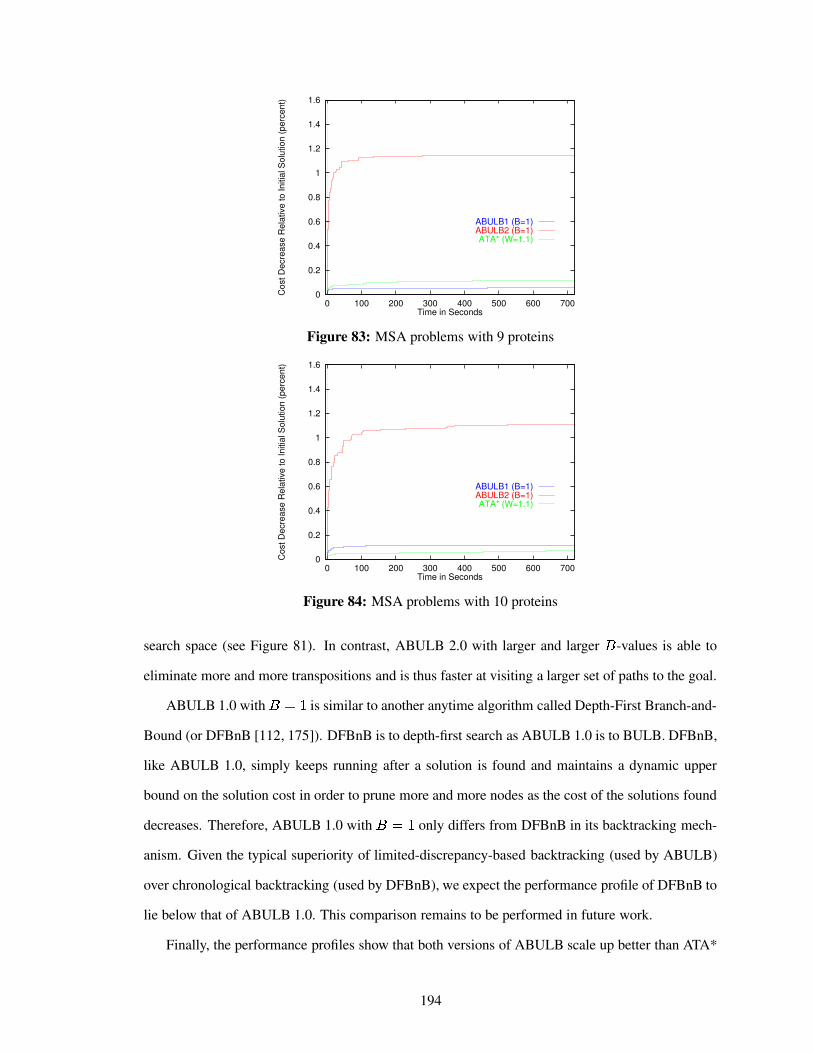
0
0.2
0.4
0.6
0.8
1
1.2
1.4
1.6
0 100 200 300 400 500 600 700
Cos
t Dec
reas
e R
elat
ive
to In
itial
Sol
utio
n (p
erce
nt)
Time in Seconds
ABULB1 (B=1)ABULB2 (B=1)ATA* (W=1.1)
Figure 83: MSA problems with 9 proteins
0
0.2
0.4
0.6
0.8
1
1.2
1.4
1.6
0 100 200 300 400 500 600 700
Cos
t Dec
reas
e R
elat
ive
to In
itial
Sol
utio
n (p
erce
nt)
Time in Seconds
ABULB1 (B=1)ABULB2 (B=1)ATA* (W=1.1)
Figure 84: MSA problems with 10 proteins
search space (see Figure 81). In contrast, ABULB 2.0 with larger and larger -values is able to
eliminate more and more transpositions and is thus faster at visiting a larger set of paths to the goal.
ABULB 1.0 with ���� is similar to another anytime algorithm called Depth-First Branch-and-
Bound (or DFBnB [112, 175]). DFBnB is to depth-first search as ABULB 1.0 is to BULB. DFBnB,
like ABULB 1.0, simply keeps running after a solution is found and maintains a dynamic upper
bound on the solution cost in order to prune more and more nodes as the cost of the solutions found
decreases. Therefore, ABULB 1.0 with C�C� only differs from DFBnB in its backtracking mech-
anism. Given the typical superiority of limited-discrepancy-based backtracking (used by ABULB)
over chronological backtracking (used by DFBnB), we expect the performance profile of DFBnB to
lie below that of ABULB 1.0. This comparison remains to be performed in future work.
Finally, the performance profiles show that both versions of ABULB scale up better than ATA*
194

0
0.2
0.4
0.6
0.8
1
1.2
1.4
1.6
0 100 200 300 400 500 600 700
Cos
t Dec
reas
e R
elat
ive
to In
itial
Sol
utio
n (p
erce
nt)
Time in Seconds
ABULB1 (B=1)ABULB2 (B=1)
Figure 85: MSA problems with 11 proteins
0
0.2
0.4
0.6
0.8
1
1.2
1.4
1.6
0 100 200 300 400 500 600 700
Cos
t Dec
reas
e R
elat
ive
to In
itial
Sol
utio
n (p
erce
nt)
Time in Seconds
ABULB1 (B=1)ABULB2 (B=1)
Figure 86: MSA problems with 12 proteins
since the latter algorithm can only solve the MSA problems with � smaller than or equal to 10.
The absence of a curve for ATA* in Figures 85 through 87 reflects the fact that ATA* runs out of
memory before finding a first solution in at least one of the instances corresponding to ��O�@�Y(3�3!�(or 13. When it does find a solution before running out of memory, ATA* reduces the solution cost
at a rate similar to that of ABULB 1.0.
To summarize our results, the ABULB algorithms scale up to larger MSA problems than the
ATA* algorithm, and ABULB 2.0 reduces the solution cost faster than ABULB 1.0 in our test
cases.
195

0
0.2
0.4
0.6
0.8
1
1.2
1.4
1.6
0 100 200 300 400 500 600 700
Cos
t Dec
reas
e R
elat
ive
to In
itial
Sol
utio
n (p
erce
nt)
Time in Seconds
ABULB1 (B=1)ABULB2 (B=1)
Figure 87: MSA problems with 13 proteins
6.9 Conclusion
In this chapter, we have used the Multiple Sequence Alignment (MSA) problem as an additional
benchmark domain for ABULB. We explained how the MSA problem of maximizing the similarity
score of an alignment of � biological sequences reduces to the shortest-path problem of minimizing
the cost of a path between two opposite corners of an � -dimensional hypercube.
Our empirical results show that, on our MSA test problems, both ABULB 1.0 and ABULB 2.0
scale up to larger problems than Anytime A*, another anytime heuristic search algorithm based on
WA*. Our results also show that ABULB 2.0 reduces the solution cost more quickly than AB-
ULB 1.0.
While our goal in this chapter was not to improve the state of the art in this domain, this is a
worthwhile goal for the future. The first step in this direction requires the study of the relevant tools
already developed within the bioinformatics community. This is no small undertaking given the
vast array of existing algorithms for this problem. However, someone familiar with this tool box
should be able to take advantage of it and to compound its power with ideas from heuristic search.
The use of heuristics to guide the search could likely be applied with benefit in the context of other
formalizations of this problem.
Most of the approaches originating in the bioinformatics community are approximations and
do not use the shortest-path formulation. For example, a popular approach is called progressive
196

multiple alignment because it progressively builds the alignment, starting with a pairwise align-
ment, by adding one complete sequence at a time to the unmodified alignment obtained so far [40].
This approach differs from the heuristic search approach since it adds one complete sequence at a
time to an existing alignment of a growing subset of sequences, while heuristic search builds an
alignment by adding one column at a time to all sequences from left to right. Progressive multiple
alignment methods have been enhanced using statistical profiles that discover and use position-
dependent information, in a way that pairwise alignments cannot do. An example of this extension
is the CLUSTALW program [163]. Other statistical, profile-based methods exist (e.g., [33]). Fi-
nally, because of the high computational complexity of the global MSA problem with gaps, a lot of
effort in bioinformatics has been spent on computationally more tractable yet very useful variants
of it. These led to such algorithms as BLAST and its variants, that are very fast at finding local
matches in large databases [2, 3]. An interesting direction for future work is to investigate the pos-
sible cross-fertilization of ideas between these progressive and local approaches on the one hand,
and heuristic search approaches on the other.
197
CHAPTER VII
CONCLUSIONS AND FUTURE WORK IN OFFLINE SEARCH
This chapter concludes the second and last part of the dissertation by summarizing our contributions
to offline search and outlining some directions for future work in this area.
7.1 Our contributions to offline search
In the second part of this dissertation (Chapters 3 through 6), we have improved on state-of-the-art
offline heuristic search methods. Our primary goal was to design new heuristic search algorithms
that scale up to larger problems. Our secondary goal was to find low-cost solutions in a reasonable
amount of time. This second part of the dissertation is itself split into two parts. First, Chap-
ters 3 and 4 introduced two new one-shot heuristic search algorithms (namely MSC-KWA* and
BULB). Second, Chapters 5 and 6 introduced a new family of anytime heuristic search algorithms
(namely the variants and combinations of ABULB and ITSA*) and their application to the multiple
sequence alignment problem. Figure 1 shows the position of our new algorithms in the space of
heuristic search algorithms, while Table 2 and the accompanying discussion demonstrate that we
have achieved both our primary and secondary goals. We now summarize in turn our contributions
to one-shot and anytime search.
7.1.1 Our contributions to one-shot search
In Chapter 3:
k We provided stronger empirical support for the improved scaling behavior of MSC-WA* over
WA* by 1) measuring its search effort, solution cost and memory consumption while varying
both the size of the commitment list and the relative weight on the h-values (the original study
kept this weight fixed), and by 2) testing it in two additional domains.
198

k We provided stronger empirical support for both the speedup and reduced memory consump-
tion (for a given solution cost) KWA* over WA* by 1) using a slightly improved implemen-
tation of KWA* that does scale it up to the 35-Puzzle (the original implementation did not)
and 2) by testing it in two additional domains.
k We showed empirically that KWA* and MSC-WA* improve WA* in two orthogonal ways.
Because of its stronger breadth-first search component (i.e., diversity), KWA* improves its
solution quality for a given level of memory consumption. Because of its stronger depth-first
search component (i.e., commitment), MSC-WA* improves its memory consumption.
k We combined the orthogonal and complementary ideas of diversity and commitment, result-
ing in the MSC-KWA* algorithm. We showed empirically that MSC-KWA* scales up to
larger domains than either KWA* or MSC-WA*. For example, in our experimental setup,
MSC-KWA* scales up to the 48-Puzzle, while KWA* and MSC-WA* only scale up to the
35-Puzzle. WA* only scales up to the 24-Puzzle.
k We discussed the similarities between MSC-KWA* and beam search. This discussion pro-
moted the role of diversity (i.e., the parallel expansion of the set of candidate nodes) in the
performance of beam search, while the initial motivation for beam search was the idea of com-
mitment. As an aside, the similarities between MSC-KWA* and beam search also motivated
our focus on beam search in the following two chapters.
In Chapter 4:
k We combined the ideas of beam search and backtracking. We showed that, when beam search
runs out of memory, backtracking is a relatively simple way (when compared to existing
memory-bounded algorithms such as SMAG*) of purging nodes from memory in order to
continue the search in another direction. Furthermore, applying backtracking to beam search
reduces the runtime over depth-first-based memory-bounded searches (such as IDA*, RBFS
or LDS) because, as increases, beam search eliminates more and more transpositions (i.e., it
detects more and more distinct paths to the same node) and thus reduces the associated node-
regeneration overhead. This first contribution is refined into the following two contributions
199

comparing the effect on the runtime of two different ways of performing backtracking with
beam search.
k We applied chronological backtracking to beam search, resulting in the DB algorithm. We
showed empirically that the runtime of DB is typically unacceptably large. This confirms the
well-known observation that chronological backtracking is not efficient when the heuristic
is misleading in nodes that are far from the goal, since chronological backtracking retracts
decisions lower in the tree (where the heuristic is often better informed) before it does so
closer to the root (where the heuristic is often less informed).
k We applied limited-discrepancy-based backtracking to beam search, resulting in the BULB
algorithm. Like DB, BULB is memory-bounded and can solve larger problems than beam
search for each value of . Furthermore, by varying the value of , BULB generalizes both
limited-discrepancy search (when � � ) and breadth-first search (when � q ). We
showed empirically in three benchmark domains that BULB not only scales up to large prob-
lems but also exhibits small runtimes (on the order of seconds or minutes) in these problems.
7.1.2 Our contributions to anytime search
In Chapter 5:
k We introduced a new local path optimization called ITSA*. ITSA* is based on a search
strategy called iterative tunneling. ITSA* is also an anytime algorithm and we showed that it
reduces the solution cost output by BULB in the 48-Puzzle and the Rubik’s Cube.
k We described and empirically evaluated different ways of transforming BULB into an any-
time algorithm, both with and without dynamic beam widths. We showed empirically that
restarting BULB with increasing values of the beam width (a variant called ABULB 2.0)
leads to a faster reduction in the solution cost than simply letting BULB run with the same
(constant) beam width after a goal is found (a variant called ABULB 1.0). ABULB 2.0 is able
to take advantage of all the available memory, while ABULB 1.0 uses less and less memory
as the solution cost decreases.
200

k To the best of our knowledge, our way of combining ABULB with ITSA* is the first success-
ful application of local (or neighborhood) search to the shortest path problem. This combina-
tion yields a larger reduction in the solution cost in the 48-Puzzle than the one obtained with
either plain ABULB or ITSA*.
In Chapter 6:
k We used the multiple sequence alignment (MSA) problem in molecular biology as an ad-
ditional benchmark domain for ABULB. We discussed the minor modifications needed for
applying ABULB to this domain.
k Our empirical results showed that, on our MSA test problems, both ABULB 1.0 and AB-
ULB 2.0 scale up to larger problems than Anytime A*, another anytime heuristic search
algorithm based on WA*. On problems that Anytime A* could solve, both variants of AB-
ULB yielded a larger decrease in solution cost. Finally, ABULB 2.0 reduced the solution cost
more quickly than ABULB 1.0.
7.2 Lessons learned and future work
In this section,we discuss three possible directions for future work.
7.2.1 Generalization of MSC-KWA* and beam search
In Chapter 3, we (unintentionally) came close to re-inventing beam search by combining the ideas
of commitment and diversity and applying them to WA*. Indeed, it was this observation (together
with the good performance of MSC-KWA*) that piqued our interest in beam search and eventually
led to our work on BULB and ABULB. We now believe that beam search is at least as good as
(and probably better than) WA* as a starting point for scaling up heuristic search. We hope that this
research will spark some renewed interest in beam search.
Furthermore, in Chapter 3, we discussed one important difference between beam search and
MSC-KWA*, namely the fact that the latter uses memory to store nodes in a reserve list while beam
search does not. Thus, MSC-KWA* can later return to a discarded node, while beam search needs
to find a new path to pruned nodes before expanding them. In this respect, the commitment (to a set
201

of candidate nodes) is stronger in beam search than it is in MSC-KWA* given the same commitment
level � . In fact, beam search and MSC-KWA* sit at two extremes on a spectrum of methods that
use reserve lists of varying lengths ª (namely, ª ��m for beam search and ª � q for MSC-
KWA*). One explanation for the better scaling of beam search in the Rubik’s Cube domain may be
that MSC-KWA* runs out of memory because of the reserve list. Thus, a smaller value of ª may
improve scaling. However, this cannot be the whole explanation given the results summarized in
Table 2 in the Towers of Hanoi domain. Making ª a parameter of the search is one way to control
the strength of the commitment.
Another dimension along which to contrast beam search and MSC-KWA* is their greediness
(or equivalently their value for ). While MSC-KWA* can explicitly vary this value, beam search
orders the set of candidate nodes according to h-values only (corresponding to ���� ). In contrast
to the breadth-first-based version of beam search we used in this research, other variants exist in
which nodes are ordered by increasing f-values (like in A*), corresponding to ���m�P � .Yet another dimension of variation is the relation between the values of � and � . In breadth-
first-based beam search, � � � , while MSC-KWA* only imposes that � be smaller than or equal
to � .
In conclusion, we have discussed four components of a search strategy (namely, its greediness
( ), its diversity ( � ), and its level ( � ) and strength ( ª ) of commitment) which can be varied to
cover a large number of variants of beam search and MSC-KWA*. The study of a general framework
for this class of approaches promises to be an interesting direction for future work.
7.2.2 Application of neighborhood search to the shortest-path problem
Another lesson learned from this research is that local search in the space of solution paths is a
promising avenue of research in anytime heuristic search. We have only scratched the surface with
ITSA* and ABULB. For example, it makes sense to take advantage of existing techniques well-
known to the Operations Research community. We discuss a few relevant issues.
First, we have used ABULB to select restart solutions when ITSA* reaches a local minimum.
Another, standard approach in neighborhood search consists of randomizing the search. One pos-
sible way to randomize heuristic search is simply to add random noise to the h-values. This is
202

expected to work well (even with noise of a small amplitude) in domains where many nodes have
the same f-values due to the fact that both g- and h-values are integral and the number of distinct
h-values is relatively small.
Second, the neighborhood searched by ITSA* is essentially constructed by a breadth-first search
around a given solution path whose depth is limited only by the available memory. Other neighbor-
hoods can of course be defined. One could perhaps use a uniform-cost search instead of a breadth-
first search by taking into account edge costs instead of simply counting edges. The search literature
contains at least one other type of neighborhood. [136] describes a post-processing method that im-
proves on a sub-optimal solution path by repeatedly selecting a sub-path of it and running A* to find
the shortest path between its start and end points. The main disadvantage of such methods is that
they require the setting of parameters such as the location of the starting state and length of these
sub-paths.
Third, it is interesting to consider the following trade-off. The larger the neighborhood, the
more likely it is to contain a local optimum of high quality, but also the more computationally
expensive it is to search. In our context, the size of the neighborhood is defined by the amount
of available memory. In the extreme case where memory is unlimited, ITSA* reduces to A* and
may take exponential time to search the neighborhood. In the intermediate case, the question arises
whether all available memory should be allocated to ITSA*. It is an empirical question whether the
improvement in solution cost is faster with a single execution of ITSA* until memory runs out, as
opposed to repeated executions of ITSA* with limited memory. If the latter setup exhibits a faster
cost reduction, then part of the available memory could be used for other purposes such as, for
example, more informed memory-based heuristics.
Fourth, another research issue is the choice of the strategy used for searching the neighbor-
hood. Neighborhood search is sometimes called iterative-improvement search [144, 1], since solu-
tion quality is improved (that is, solution cost is reduced) by iteratively jumping from one path to
another one in the neighborhood. This general paradigm leaves open the question of how to select
the next solution path within the neighborhood. ITSA* follows a best-improvement [1] or steepest-
descent [130] strategy, since it uses a variant of A* to select the solution of lowest cost within the
neighborhood. Alternatively, a first-improvement strategy would stop searching the neighborhood
203

when any solution is found with a lower cost than the current solution.
Finally, the choices of (re)start solutions and neighborhoods may interfere with each other. [130]
defines the strength of a neighborhood (of a given size) as the average quality of the local optima that
are reached when searching the neighborhood. However, the quality of the attainable local optima
may depend on the starting solution. An interesting direction for research is to study empirically
how the strength of a neighborhood correlates with the average quality of the starting solutions.
Ideally, a strong neighborhood would be weakly correlated with the quality of the starting solutions.
One can thus compare the strength of different neighborhood structures using multiple methods for
selecting restarts.
7.2.3 Domain-specific extensions
In Chapter 6, we have used the Multiple Sequence Alignment problem as an additional benchmark
domain for ABULB. Our goal in this dissertation was not to improve the state of the art in this
domain. Nevertheless, this is a worthwhile goal for the future. The first step in this direction requires
the study of the relevant tools already developed within the bioinformatics community. This is no
small undertaking given the vast array of existing algorithms for this problem. However, someone
familiar with this tool box should be able to take advantage of it and to compound its power with
ideas from heuristic search. The use of heuristics to guide the search could likely be applied with
benefit in the context of other formalizations of this problem. For example, existing specialized
algorithms for this problem build the alignment incrementally by adding one sequence at a time to
an already completed sub-alignment. This process is in contrast to the way heuristic search builds
an alignment, namely column by column while considering all sequences simultaneously (recall
that each state in our search space represents a partial alignment of all sequences up to a certain
prefix of the sequences and that each action consumes either one or zero letter in each sequence).
Nevertheless, it may be possible to use heuristic search in a different space in which each state
represents a complete alignment of a sub-set of sequences and each action adds one full sequence
to the alignment under construction.
Finally, symbolic planning is another application area where heuristic search has had great suc-
cess [14, 13, 12, 66, 159, 92, 116, 93]. Applications of heuristic search to symbolic planning have
204

used variants of both WA* and beam search. We believe that it will be advantageous in terms of
scaling to adapt our beam-search-based ideas to these tasks.
205

APPENDIX A
FORMAL PROOFS FOR FALCONS �
A.1 Introduction
This Appendix contains the formal proofs for the theoretical results pertaining to FALCONS stated
in Section 2.6.2. The proofs are preceded by some definitions, notation, and assumptions.
A.2 Definitions
& , :�r'sIucvws , :<xcy ubz , :3;�=f=@%�:Y, , [�� . � %�:�, , =@%�:�(c: D , , � � %�:�, , : � %�:�, , � %�:Y, , � %�:Y, , � � %�:Y, , � � %�:�, , �G%�:Y, , and � � %�:Y,are defined in Section 2.2. Furthermore:
D1 G-values are admissible iff ml� � %�:Y,¾�Ð: � %�:Y, for all states : .
D2 H-values are admissible iff ml� � %�:Y,¾� � � %�:�, for all states : .
D3 G-values are consistent iff � %�:{r'sIucv¨sw,6��m and m�� � %�:<D�,¾� � %�:Y, � =Y%�:�(c:<DZ, for all states : with
:¸��":�r'sIucvws and : D 7�:<;>=?=@%�:�, , that is, if they satisfy the triangle inequality.
D4 H-values are consistent iff � %�:�xcy ubz , � m and m�� � %�:Y,^�9=Y%�:�(c:<D�, ��� %�:3D�, for all states : with
:¸��":<xcy ucz and : D 7�:<;>=?=@%�:�, , that is, if they satisfy the triangle inequality.
D5 The state space & is safely explorable iff the goal distances of all states are finite
A.3 Notation
Superscripts of f-, g-, and h-values. In the following proofs, � s %�:�, (resp. � s %�:Y, and � s %�:�, ) refers
to the f-value (resp. g-value and h-value) of state : before the ÿ � � value update, that is, before
Step 3 (Figure 88) of iteration ÿ � � . Thus, � N %�:Y, and � N %�:�, are the initial g- and h-values of state :before Step 3 of iteration 1.
�This Appendix is a modified version of [50].
206

1. : := :�rtsIu+vws2. : D := arg �� I¡ r'¢ ¢�£@r'¤�¥'¥w¦Xr¨§ �G%�: D D , ,
where �G%�: D D , := ��¬�·% � %�: D D , ��� %�: D D ,b( � %�:�rtsIu+vws¨,4, [F-CALC]Break ties in favor of a successor :�D with the smallest value of =@%�:{(c:�D�, ��� %�:3D�, [TB]Break remaining ties arbitrarily (but systematically « ) [TB2]
3. � %�:�, := if ( :À�": r'sIucvws ) then � %�:�,else ��¬�H% � %�:Y, ,
�� I¡ r ¢ ¢ £fRQv4¹¨º?¦Xr¨§ % � %�:<D DI, � =@%�:3D D©(c:�,4, ,��¬� rt¢ ¢�£@r'¤<¥t¥w¦Xr¨§ % � %�:<D D�,)Á�=Y%�:�(c:<D DI,4,4,
[G-UPDATE]
� %�:Y, := if ( :ª�":<xcy ucz ) then � %�:Y,else ��¬� % � %�:�, ,
�� I¡ rt¢ ¢j£Yrt¤<¥'¥w¦Zr³§ %©=@%�:�(c:3D D�, ��� %�:3D DI,4, ,��¬� r ¢ ¢ £?RQv4¹³º?¦Zr³§ % � %�:<D Dj,AÁ�=Y%�:<D D©(c:�,4,4,
[H-UPDATE]
4. If ( :E�":<xcy ucz ) then stop successfully
5. : := :<D6. Go to Line 2
Figure 88: The FALCONS algorithm
Subscripts of state variables. :Ys refers to the current state before Step 5 (Figure 88) of iteration
ÿ � � . Thus, : N �": r'sIucvws .
A.4 Assumptions
Our results hold under the following assumptions:
A1 The state space & is finite.
A2 The state space & is safely explorable.
A3 All actions costs are positive.
A4 The initial g- and h- values are admissible.
A5 The initial g-values are consistent.
Assumption A5 is only used for results pertaining to the use of FALCONS without G-UPDATE.
Furthermore, A5 implies the part of A4 that pertains to the g-values, since the consistency of the
¯Systematic tie-breaking is defined in Section 2.3.
207

g-values implies their admissibility. In practice, most admissible heuristic values are also consistent.
Indeed, all of the heuristic values described in Section 2.7.1 are consistent.
A.5 Proofs
We first prove some lemmata pertaining to properties of the g-, h-, and f-values that are guaranteed to
hold during the execution of FALCONS. Then, we prove that each trial of FALCONS is guaranteed
to terminate (Theorems 1 and 2), that each run of FALCONS is also guaranteed to terminate, that
is, FALCONS always converges to a unique path (Lemma 6 and Corollary 6), and finally that the
path FALCONS converges to at the end of each run is a minimum-cost path (Theorems 3 and 4).
When appropriate, the following lemmata and theorems are accompanied by corollaries that extend
the results to FALCONS without the G-UPDATE rule.
Lemma 1
1. Under assumptions A1-4, FALCONS cannot decrease the g-values.
2. Under assumptions A1-4, FALCONS cannot decrease the h-values.
Proof:
Since only Step 3 of FALCONS modifies the heuristic values, we need only consider that step. Let
ÿ¾7 M��Y(c!�(cÌ�(QPQPQP0T be the number of the current iteration. Let : be any state in & .
1. Proof for G-UPDATE
Case (i): :ª�":<sIf :À�": rtsIu+vws then � s ! 1 %�:�,�� `�� ö �������� � s %�:Y, , else
� s ! 1 %�:Y,�� `�� ö �������� L �!�"####$ ####%� s %�:�,b(�¸ I¡ r ¢ ¢ £?RQv4¹³º?¦Zr³§ % � s %�:<D DI, � =@%�:<D D0(c:Y,4,b(�¸¬� rt¢ ¢�£Yrt¤<¥'¥w¦Zr³§ % � s %�: D D ,)ÁÑ=@%�:�(c: D D ,4,
&'####(####)*,+.- g0/ -214365
~ � s %�:Y,bP
Case (ii): :��� :<sIn this case, � %�:Y, is not updated, and thus � s ! 1 %�:�,6� � s %�:�, .
Therefore in both cases, Udÿ¾7 M��Y(c!�(cÌ�(QPQPQP0T{(c:�7Ä&¾� � s ! 1 %�:Y,¶~ � s %�:Y, .
208
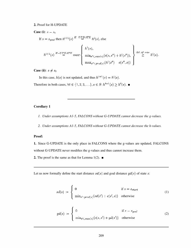
2. Proof for H-UPDATE
Case (i): :ª�":<sIf :À�":<xcy ubz then � s ! 1 %�:�,�7 `�� ö �������� � s %�:Y, , else
� s ! 1 %�:Y,�7 `�� ö ���2���� L �8�"####$ ####%� s %�:Y,b(�� I¡ r ¢ ¢ £Yrt¤<¥'¥w¦Zr³§ %©=Y%�:�(c:<D D�, ��� s %�:3D D�,4,b(��¬� r'¢ ¢I£?RQv4¹³ºQ¦Xr¨§ % � s %�: D D ,2Á�=Y%�: D D (c:�,4,
&'####(####)*,+.- g0/ -214365
~ � s %�:Y,bP
Case (ii): :��� :<sIn this case, � %�:Y, is not updated, and thus � s ! 1 %�:Y,6� � s %�:Y, .
Therefore in both cases, Udÿ¾7 M��Y(c!�(cÌ�(QPQPQP0T{(c:�7Ä&¾� � s ! 1 %�:Y,¾~ � s %�:Y, .
Corollary 1
1. Under assumptions A1-5, FALCONS without G-UPDATE cannot decrease the g-values.
2. Under assumptions A1-5, FALCONS without G-UPDATE cannot decrease the h-values.
Proof:
1. Since G-UPDATE is the only place in FALCONS where the g-values are updated, FALCONS
without G-UPDATE never modifies the g-values and thus cannot increase them.
2. The proof is the same as that for Lemma 1(2).
Let us now formally define the start distance : � %�:�, and goal distance � � %�:�, of state : :
: � %�:Y, :=
"#$ #% m if :ª�":�r'sIucv¨s�� I¡ rt¢I£fR3vw¹¨º?¦Zr³§ %�: � %�:3DI, � =@%�:<Dj(c:Y,4, otherwise
(1)
� � %�:�, :=
"#$ #% m if :ª�":<xcy ucz�� I¡ rt¢I£Yrt¤<¥'¥4¦Xr¨§ %©=Y%�:�(c:<DI, ��� � %�:<D�,4, otherwise
(2)
209

Lemma 2
1. Under assumptions A1-4, the g-values remain admissible during the execution of FALCONS.
2. Under assumptions A1-4, the h-values remain admissible during the execution of FALCONS.
Proof:
1. Proof by induction on ÿ .At ÿG�"m , assumption A4 guarantees that UÃ:�7�& : � N %�:Y, is admissible.
Assume that the induction hypothesis holds at the beginning of iteration ÿ :
UÃ:�7�&)( � s %�:Y, V³:9� � L V³:�:3V/«b� . (3)
Let us prove that UH:E7�&)( � s ! 1 %�:Y, is admissible as well. Let : be any state in & .
If :"��$:<s , then � %�:Y, is not modified during iteration ÿ . Therefore, � s ! 1 %�:Y, � � s %�:Y, , which
is admissible by Equation 3. If :� :Ys , then � %�:�, is only modified by G-UPDATE (Step 3 of
FALCONS). Now, if :ª�":YrtsIu+vws , then � s ! 1 %�:�, � `�� ö �������� � s %�:Y, , which is admissible by Equation 3.
Therefore, we need only consider the situation where :À�":{sp��":�rtsIu+vws , for which it holds that:
� s ! 1 %�:�, � `�� ö �������� L �8�"####$ ####%� s %�:�,b(�¸ I¡ r'¢ ¢I£?RQv4¹³ºQ¦Xr¨§ % � s %�: D D , � =Y%�: D D (c:Y,4,b(�¸¬� r ¢ ¢ £Yrt¤<¥'¥4¦Xr¨§ % � s %�:<D DI,)Á�=@%�:�(c:3D D�,4,
& ####(####)
We distinguish 3 cases, depending on which of the 3 arguments of max is the largest.
:�;=< :4[ := arg �� I¡r ¢ ¢ £?RQv4¹³ºQ¦Xr¨§ %� s %�: D D , � =@%�: D D (c:�,4,bP (4)
:>;=< :�: := arg ��¬�r'¢ ¢I£@r'¤�¥'¥w¦Xr¨§ %� s %�: D D ,AÁÑ=@%�:{(c: D D ,4,bP (5)
Case (i): � s ! 1 %�:Y,6� � s %�:Y,Then, by Equation 3, � s ! 1 %�:Y, is admissible.
Case (ii):
� s ! 1 %�:�, � � s %�:+[Ã, � =@%�:4[A(c:�, (6)
Proof by contradiction.
:�;=< :�: � := arg �� I¡r'¢ ¢�£?RQv4¹³ºQ¦Xr¨§ %�:� %�: D D , � =@%�: D D (c:Y,4,bP (7)
?A@8B�C (�: � %�:Y,G�": � %�:�: � , � =@%�:�: � (c:Y,bP (8)
210

(Note that Equation 8 implies that :�: � ��": .) Now, assume � s ! 1 %�:Y,¶|Ð: � %�:Y, .This, combined with Equations 6 and 8, yields
� s %�:4[Ã, � =@%�:4[·(c:Y,G� � s ! 1 %�:�,¶|Ð: � %�:Y,6�": � %�:�: � , � =@%�:�: � (c:�,bP (9)
But, since � s %�:�: � , is admissible by Equation 3, : � %�:�: � , � =@%�:�: � (c:�,p~ � s %�:�: � , � =@%�:�: � (c:Y, , which,
combined with Equation 9, implies: � s %�:+[Ã, � =@%�:+[·(c:�,¶| � s %�:�: � , � =Y%�:�: � (c:Y, . The latter contradicts
Equation 4. Therefore, � s ! 1 %�:�,¶�Ð: � %�:Y, , i.e. � s ! 1 %�:Y, is admissible.
Case (iii):
� s ! 1 %�:Y,6� � s %�:�:Y,AÁÑ=@%�:{(c:�:Y, (10)
(Note that Equation 10 implies that :�:��� : . Otherwise, � %�:�,�� � %�:�:Y, would strictly decrease
between ÿ and ÿ � � , since =@%�:�(c:�:Y, � »| m .) From � s %�:�:Y,ED8FHG 36IKJ /ML^»� : � %�:�:Y, and : � %�:�:Y,*0+�- gH/ - r³º
�: � %�:Y, � =@%�:{(c:�:�, , we obtain � s %�:�:Y,À�K: � %�:Y, � =@%�:{(c:�:Y, , or equivalently � s %�:�:�,6Á®=Y%�:�(c:�:�,À��: � %�:�, ,which, combined with Equation 10, yields � s ! 1 %�:Y,¾�o: � %�:Y, . Therefore, � s ! 1 %�:Y, is admissible.
In conclusion, � s ! 1 %�:�, is admissible in all cases.
2. Proof by induction on ÿ .At ÿG�"m , assumption A4 guarantees that UÃ:�7�& : � N %�:Y, is admissible.
Assume that the induction hypothesis holds at the beginning of iteration ÿ :
UÃ: 7�&¾� � s %�:Y, V³:N� � L V³:�:3V�«f� . (11)
Let us prove that UH:E7�&¾� � s ! 1 %�:Y, is admissible as well. Let : be any state in & .
If :��� : s , then � %�:�, is not modified during iteration ÿ . Therefore, � s ! 1 %�:Y,�� � s %�:�, , which is
admissible by Equation 11. If :��C:Ys , then � %�:Y, is only modified by H-UPDATE (Step 3 of FAL-
CONS). Now, if :¸��:�xcy ucz , then � s ! 1 %�:Y, 7 `�� ö �������� � s %�:Y, , which is admissible by Equation 11.
Therefore, we need only consider the situation where :À�":{sp��":3xby ubz , for which it holds that:
� s ! 1 %�:Y, 7 `�� ö �������� L �8�"####$ ####%� s %�:Y,b(�� I¡ rt¢ ¢�£Yrt¤<¥'¥w¦Zr³§ %©=@%�:�(c: D D , ��� s %�: D D ,4,b(��¬� r ¢ ¢ £?RQv4¹³º?¦Zr³§ % � s %�:<D DI,)ÁÑ=@%�:<D D0(c:Y,4,
& ####(####)
211

We distinguish 3 cases, depending on which of the 3 arguments of max is the largest.
:�;=< :�: := arg �� I¡rt¢ ¢�£Yrt¤<¥'¥w¦Zr³§ %©=@%�:{(c: D D ,�Â� s %�: D D ,4,bP (12)
:�;=< :+[ := arg �¸¬�rt¢ ¢�£fRQv4¹¨º?¦Xr¨§ %� s %�: D D ,)ÁÑ=@%�: D D (c:Y,4,bP (13)
Case (i): � s ! 1 %�:Y,6� � s %�:�,Then, by Equation 11, � s ! 1 %�:Y, is admissible.
Case (ii):
� s ! 1 %�:Y,6��=@%�:�(c:�:Y, ��� s %�:�:Y, (14)
Proof by contradiction.
:>;=< : � � := arg �� I¡rt¢ ¢�£Yrt¤<¥'¥w¦Zr³§ %©=Y%�:�(c: D D ,��� � %�: D D ,4,bP (15)
?A@OB2C ( � � %�:Y,6��=@%�:{(c: � � , ��� � %�: � � ,bP (16)
(Note that Equation 16 implies that : � � ��": .) Now, assume � s ! 1 %�:Y,¾| � � %�:�, .This, combined with Equations 14 and 16, yields
=@%�:�(c:�:Y, ��� s %�:�:Y,G� � s ! 1 %�:Y,¾| � � %�:Y,6��=@%�:{(c: � � , ��� � %�: � � ,bP (17)
But, since � s %�: � � , is admissible by Equation 11, =@%�:{(c: � � , ��� � %�: � � ,p~Ð=Y%�:�(c: � � , � � s %�: � � , , which,
combined with Equation 17, implies =Y%�:�(c:�:�, ��� s %�:�:�,¶|o=@%�:�(c: � � , ��� s %�: � � , . The latter contradicts
Equation 12. Therefore, � s ! 1 %�:�,¶� � � %�:Y, , i.e. � s ! 1 %�:�, is admissible.
Case (iii):
� s ! 1 %�:�, � � s %�:+[Ã,AÁÑ=@%�:+[·(c:�, (18)
(Note that Equation 18 implies that :+[Ï�� : . Otherwise, � %�:Y,J� � %�:+[Ã, would strictly decrease
between ÿ and ÿ � � , since =@%�:+[·(c:Y, � »|�m .) From � s %�:4[Ã, D8FHG 36IPJ /ML 141� � � %�:+[Ã, and � � %�:+[Ã,*,+.- g0/ - x º
�=@%�:4[A(c:�, �®� � %�:Y, , we obtain � s %�:+[Ã,^�9=@%�:4[·(c:Y, �_� � %�:Y, , or equivalently � s %�:+[Ã,)Á_=@%�:4[·(c:Y,^� � � %�:�, ,which, combined with Equation 18, yields � s ! 1 %�:�,¶� � � %�:Y, . Therefore, � s ! 1 %�:Y, is admissible.
In conclusion, � s ! 1 %�:Y, is admissible in all cases.
212
Corollary 2
1. Under assumptions A1-5, the g-values remain admissible during the execution of FALCONS
without G-UPDATE.
2. Under assumptions A1-5, the h-values remain admissible during the execution of FALCONS
without G-UPDATE.
Proof:
1. Since G-UPDATE in Step 3 of FALCONS is the only step that modifies the g-values, FALCONS
without G-UPDATE does not modify the g-values, and the g-values thus remain admissible.
2. Since G-UPDATE does not have any effect on the h-values, its absence in FALCONS does not
make a difference in whether the h-values remain admissible. Therefore, this proof is the same as
that for Lemma 2(2).
Lemma 3 Under assumptions A1-4, a trial of FALCONS could only run forever if, from some time
on, it repeatedly moved along a finite cyclic path without modifying any of the g- and h-values in
the cycle.
Proof: Consider the h-values. Lemma 1(2) guarantees that, on every transition, the h-value of
the current state : can only increase or stay the same. In addition, Lemma 2(2) provides an upper
bound on � %�:�, , namely � � %�:Y, (which is finite, by A2). This means that the maximum number of
strict increases of � %�:�, is finite. This reasoning holds for all states : in & . And since & is finite (A1),
we infer that the maximum total number (over & ) of strict increases of h-values by H-UPDATE
is finite. The same reasoning applies to G-UPDATE for the g-values. In conclusion, there is a
maximum, finite number of strict increases possible for both the g- and h-values. Therefore, if
FALCONS never terminates, there must be a point in time, say ø , after which no g- nor h-values are
modified. Now, we prove that from some time ø 1 on ( ø 1 ~pø ), it must be the case that FALCONS
repeatedly moves along a cycle. Let : 1 denote the first state to be visited twice after time ø ( : 1
must exist, by A1). Let ø 1 (resp. ø 5 ) denote the instant in time at which : 1 is reached for the first
(resp. second) time after time T. By definition, ø)5�~�ø)18~æø . Let � be the sequence of states
213

(starting with : 1 ) traveled through in the time interval [ ø61 , øÃ5 ). From time ø21 on, the cycle � is
repeatedly followed by FALCONS. The reason for this is that no values in the state space changes
after time ø (and therefore after time ø61 ) and systematic tie-breaking (TB2) ensures that FALCONS
will thereafter always choose the same successor at every decision point.
Corollary 3 Under assumptions A1-5, a trial of FALCONS without G-UPDATE could only run
forever if, from some time on, it repeatedly moved along a finite cyclic path without modifying any
of the g- and h-values in the cycle.
Proof: This proof is identical to that of Lemma 3, except that the finite number of strict increases
of the g-values (namely zero) directly follows from the fact that FALCONS without G-UPDATE
never modifies the g-values.
Lemma 4 Under assumptions A1-4, assume that FALCONS makes a transition from a state :as to
a state :<s ! 1 without modifying the g- and h-values of :Ys . Let : D D := �a� � L V'� rt¢I£@r'¤<¥t¥w¦XrRQ�§ %©=@%�:<s4(c: D , �� s %�:<DI,4, . Then, :<D D is such that:
1. � s %�: D D ,¶� � s %�:3s³,AÁÑ=@%�:<s4(c: D D , ,
2. � s %�:3D DI,¾� � s %�: s , � =@%�: s (c:3D DI, ,
3. � s %�:<D DI,¶�9� s %�:<s³, ,
4. � s %�:<s ! 1f,¾�Ð� s %�: D D , , and
5. if � s %�:3s³,^�Ð� s %�:�rtsIu+vws³, , then � s %�:3s ! 1b,¾�9� s %�:�rtsIu+vws³, .
Proof:
First, note that :�s^��":<xcy ucz . Otherwise, FALCONS would stop in :Ys .Second, note that : D D ��}:<s . If that was not the case, it would hold that � s ! 1 %�:3s³, 7 `�� ö �������~
�� I¡ r ¢ £@r'¤�¥'¥w¦XrRQ�§ %©=Y%�:<s4(c:<DZ, �®� s %�:3DI,4, ��S ¤<ucs ] y ôE1b�� =Y%�:<s4(c:<s³, �®� s %�:3s³, , which would imply that � s ! 1 %�:<s³,·Á
214
� s %�:<s³,¶~o=@%�:<s4(c:3s³, � »|�m and contradict our assumption that � s ! 1 %�:<s³,6� � s %�:<s³, . Thus, : D D ��":3s .:�;=< : D D := �a� � L V'� rt¢I£Yrt¤<¥'¥4¦Xr Q § %©=@%�:<s+(c: D , ��� s %�: D ,4,bP (19)
1. Proof by contradiction.
Assume � s %�:<st,®n�=Y%�:<s4(c:<D DI, �C� s %�:<D DI, . This, together with Equation 19, implies that � s %�:<s³,_n�� I¡ rt¢I£@r'¤�¥'¥w¦XrRQ�§ %©=Y%�:<s4(c: D , �C� s %�: D ,4, 7 `�� ö ���2���� � s ! 1 %�:3s³, , which contradicts � s ! 1 %�:3st,Â� � s %�:3s³, .Therefore, :<D D must satisfy � s %�:<s³,¶~o=@%�:3s4(c:<D D�, �_� s %�:<D D�, , or equivalently � s %�:<D D�,¶� � s %�:3s³,·Á =@%�:3sw(c:<D DI, .2. Case (i): :�sA�":�rtsIu+vwsFirst, note that
Udÿ¶7 M��Y(c!�(cÌ�(QPQPQP0T{� � s %�:�rtsIu+vws³,6�"m (20)
follows from the fact that initially admissible g-values (A4) remain admissible (Lemma 2(1)).
� s %�: D D ,�T ¹�UVU¶uG5f¦j1³§� : � %�: D D , and : � %�: D D ,*0+�- gH/ - r³º
� : � %�:3st, � =@%�:3sw(c: D D ,ª�O=@%�:3s4(c: D D , imply that � s %�: D D , �=@%�:3s4(c:<D DZ, or equivalently � s %�:<D DZ,¾�Ðm � =@%�:3s4(c:<D DI, �>S ¤�u+s ] y ô 54N� � s %�:�r'sIucvws³, � =@%�:3s+(c:<D DZ, � � s %�:<s³, � =@%�:3s4(c:<D DI, .Case (ii): :<sp�� :�rtsIu+vws (Proof by contradiction)
Assume � s %�:<st,¾n � s %�:<D D�,AÁÑ=@%�:3s4(c:<D DI, .This implies that � s %�:<s³, n���¬� r ¢ £@r'¤�¥'¥w¦Xr Q § % � s %�: D ,¶Á�=@%�:3s4(c: D ,4, � `�� ö ���2���� � s ! 1 %�:3s³, , which contra-
dicts the assumption that � s ! 1 %�: s , � � s %�: s , . Thus, � s %�: s ,�~ � s %�:<D DI,ÎÁ9=@%�: s (c:3D D�, or equivalently
� s %�: D D ,¶� � s %�:3s³, � =@%�:3sw(c: D D , .3. From Results 1 and 2 above, we have � s %�:3D D�, �Â� s %�:3D DI, � � s %�: s , � =Y%�: s (c:<D D�, �o� s %�: s ,)Á�=@%�: s (c:3D D�,or equivalently � s %�: D D , �K� s %�: D D ,�� � s %�:<s³, ��� s %�:3s³, . Thus, L �!�2% � s %�:�rtsIu+vws³,b( � s %�: D D , � � s %�: D D ,4,��L �8�)% � s %�: rtsIu+vws ,b( � s %�: s , ��� s %�: s ,4, which, by F-CALC, is equivalent to � s %�:<D DZ,¾�9� s %�: s , .4. Since FALCONS chooses :�s ! 1 as the next state, it must hold that � s %�:3s ! 1f,^�Ð� s %�: D D , .5. Assume � s %�: s ,¶�Ð� s %�: rtsIu+vws , . This, together with Result 3 above, implies that
� s %�: D D ,¾�Ð� s %�:�r'sIucvws³,bP (21)
Since FALCONS chooses to move to : s ! 1 , it must be the case that � s %�: s ! 1 ,���� s %�:<D D�, , which,
together with Equation 21, yields � s %�:<s ! 1f,¾�Ð� s %�:�rtsIu+vws³, .
215

Corollary 4 Under assumptions A1-5, assume that FALCONS without G-UPDATE makes a
transition from a state :�s to a state :<s ! 1 without modifying the g- and h-values of :Ys . Let
: D D := �a� � L V'� rt¢I£@r'¤<¥t¥w¦XrRQj§ %©=Y%�:<s4(c: D , �Â� s %�: D ,4, . Then, : D D is such that:
1. � s %�: D D ,¶� � s %�:3s³,AÁÑ=@%�:<s4(c: D D , ,
2. � s %�: D D ,¾� � s %�:<st, � =@%�:<s4(c: D D , ,
3. � s %�: D D ,¶�9� s %�:<s³, ,
4. � s %�:<s ! 1f,¾�Ð� s %�: D D , , and
5. if � s %�:3s³,^�Ð� s %�:�rtsIu+vws³, , then � s %�:3s ! 1b,¾�9� s %�:�rtsIu+vws³, .
Proof:
For the same reasons as in the proof for Lemma 4, :@s^��":3xby ubz and : D D ��":<s . In addition, the g-values
are never modified.
1. This proof is the same as that for Lemma 4(1).
2. Case (i): : s �": rtsIu+vwsThis proof is the same as that for Lemma 4(2), except that Equation 20 is now true because of A4
and the absence of G-UPDATE, and that we use Corollary 2(1) instead of Lemma 2(1).
Case (ii): :<sp�� :�rtsIu+vws� s %�:<D DI,�� � s %�: s , � =Y%�: s (c:3D D�, directly follows from A5 and the definition of the consistency of the
g-values.
3. This proof is the same as that for Lemma 4(3) above.
4. This proof is the same as that for Lemma 4(4) above.
5. This proof is the same as that for Lemma 4(5) above.
Lemma 5 Under assumptions A1-4, assume that FALCONS follows a path ì starting in any state
: 1 without modifying the g- and h-values of any state on ì . If �G%�: 1 ,^�Ð�G%�:�rtsIu+vwst, , then for all states
: on ì ,
�G%�:Y, �Ð�G%�:�r'sIucv¨s³,bP (22)
216

Proof: Proof by induction on the distance of : from : 1 on ì .
If :ª�": 1 , then �G%�:Y,G�"�G%�: 1 ,¾�Ð�G%�:�r'sIucvws', . So, Equation 22 trivially holds for : 1 .Assume that : is any state on ì but the last one. Then, : has a successor : D on ì . Lemma 4(5)
directly allows us to infer that, if Equation 22 holds for : , then it also holds for :aD .
Corollary 5 Under assumptions A1-5, assume that FALCONS without G-UPDATE follows a path
ì starting in any state : 1 without modifying the g- and h-values of any state on ì . If �G%�: 1 , ��G%�:�r'sIucv¨st, , then for all states : on ì , : on ì ,
�G%�:Y, �Ð�G%�: r'sIucv¨s ,bP (23)
Proof: The proof is the same as that for Lemma 5, except that it uses Corollary 4(5) instead of
Lemma 4(5).
Lemma 6 Under assumptions A1-4, at all times t during the execution of FALCONS, � s %�: rtsIu+vws ,G�� s %�:�rtsIu+vws³, .
Proof:
� s %�:�rtsIu+vws³, W `�X � T X� L �8�)% � s %�:�rtsIu+vws³, � � s %�:�r'sIucvws³,b( � s %�:�r'sIucvws³,4, � ¿ ! T ¹RUYU¾u65f¦�1³§� L �8�)%©m �� s %�:�rtsIu+vws³,b( � s %�:�rtsIu+vws³,4,6� � s %�:�rtsIu+vws³, .
Corollary 6 Under assumptions A1-5, at all times t during the execution of FALCONS without
G-UPDATE, � s %�:�rtsIu+vws³,6� � s %�:�rtsIu+vws³, .
Proof:
The proof is the same as that for Lemma 6, except that it uses Corollary 2(1) instead of
Lemma 2(1).
217
Theorem 4 (Termination 1) Under assumptions A1-4, each trial of FALCONS is guaranteed to
terminate.
Proof: Proof by contradiction.
If FALCONS cycles forever then there exists a finite cyclic path ì along which the g- and h-values
do not change from some time T on (Lemma 3). In the following, we can drop the superscripts on
the h- and f-values since they do not change after time T.
We distinguish two cases. Either all states on ì have f-values smaller than or equal to �G%�: r'sIucvws³, , or
all states on ì have � values greater than �G%�:{rtsIu+vwst, . These are the only two possible cases. Indeed,
if there is at least one state : 1 on ì such that �G%�: 1 ,E�K�G%�:�rtsIu+vws³, , then all states following : 1 on ìwill also have an f-value smaller than or equal to �G%�:�rtsIu+vws³, (by Lemma 5). But, since ì is cyclic,
every state : on ì follows : 1 and therefore satisfies �G%�:Y,¶�K%�:@r'sIucv¨s³, .Case (i): For all states :�s on the cycle, �G%�:�st,¾|Ð�G%�:�rtsIu+vwst, .In this case, it must hold that for all successors : D of all states in the cycle, �G%�: D ,�|��G%�:�r'sIucvws', .Otherwise, FALCONS would choose as next state a successor with �G%�:�DZ,�� �G%�:�rtsIu+vwst, and thus
leave the cycle.
Let : s be any state on this cycle, : s ! 1 be the successor of : on the cycle, and
: D D := �a� � L V'� rt¢I£@r'¤<¥t¥w¦Xr Q § %©=Y%�:<s4(c: D , �Â� %�: D ,4, .By Lemma 4(3&4), �G%�: s ! 1 ,¶�Ð�G%�: s , , i.e. the f-values cannot increase along a transition. Therefore
they cannot decrease either because otherwise they would have to increase again before the end of
the cycle. So the f-values of all states on the cycle are the same and in particular �G%�: s ! 1 ,���G%�: s ,which, combined with Lemma 4(3&4) yields �G%�:@s ! 1b,6�"�G%�: D D ,6���G%�:3st, . Since FALCONS chooses
: s ! 1 as the next state, =@%�: s (c: s ! 1 , ��� %�: s ! 1 , ��Z�/=@%�: s (c:<D D�, ��� %�:3D Dj, . By definition of :�D D and H-UPDATE
(since � %�:<s³, does not change), =@%�:�s4(c:3D D�, �Ð� %�:<D DZ,ª� � %�:<s³, Combining the two previous inequalities
yields =Y%�: s (c: s ! 1 , �o� %�: s ! 1 ,p� � %�: s , . Since =@%�: s (c: s ! 1 , � »|Om , it follows that � %�: s ! 1 ,În � %�: s , . This
means that the h-value strictly decreases along this and therefore all transitions on the cycle, which
is impossible.
Case (ii): For all states :�s on the cycle, �G%�:�st,¾�Ð�G%�:�rtsIu+vwst, .Let : s be any state on the cycle. Let : s ! 1 be the successor of : on the cycle and
:<D D := �a� � L V'� rt¢I£@r'¤<¥t¥w¦Xr Q § %©=Y%�:<s4(c:<DZ, �Â� %�:<DZ,4, .
218

Now, �G%�:<D DI,[T ¹�UVU¶u ¿ ¦X»+§� �G%�: s , and �G%�: s ,9� �G%�: rtsIu+vws , imply that �G%�:�D DI,9� �G%�: rtsIu+vws , T ¹RUYU¾u6½�� %�:�rtsIu+vws³, , which, combined with �G%�: D D , W `�X � T X~ � %�:�r'sIucvws¨, , yields
�G%�: D D ,6� � %�:�r'sIucv¨s³,bP (24)
Furthermore, �G%�: s ! 1 , T ¹�UVU¶u ¿ ¦XÅ+§� �G%�: rtsIu+vws , T ¹�UVU¶u6½� � %�: rtsIu+vws , implies, together with
�G%�:<s ! 1c, W `�X � T X~ � %�:�rtsIu+vws³, , that �G%�:<s ! 1f,ª� � %�:�rtsIu+vws³, . Combining this equation with Equation 24
yields �G%�: D D , ���G%�:3s ! 1b, . Now, =@%�:<s4(c:<s ! 1f, �Â� %�:3s ! 1f, �\Z��=@%�:<s4(c: D D , �Â� %�: D D , . In addition, since � %�:�s³,does not change after the update, we know that =@%�:@s4(c:3D DI, ��� %�:<D D�,l� � %�:3s³, . Chaining the two to-
gether, we get =@%�:�s4(c:<s ! 1f, � � %�:<s ! 1f,¾� � %�:3s³, or equivalently � %�:�s ! 1f,¶� � %�:<s³,aÁ¸=@%�:3sc(c:3s ! 1b,¾n � %�:3s³, ,since =Y%�:�s4(c:3s ! 1f, � »|�m . This means that the h-value strictly decreases along this and therefore all
transitions in the cycle, which is impossible.
Theorem 5 (Termination 2) Under assumptions A1-5, each trial of FALCONS without G-
UPDATE is guaranteed to terminate.
Proof: The proof for this theorem is the same as that for Theorem 4 except that it uses the corollaries
instead of the lemmata with the corresponding numbers.
Lemma 7 (Convergence) Under assumptions A1-4, assume FALCONS is reset to :�rtsIu+vws at the end
of each trial and the g- and h-values are kept from each trial to the next. Then, from some time on,
FALCONS will always follow the same path.
Proof:
Theorem 4 above has established that each trial of FALCONS will always terminate. We now
assume that FALCONS is reset into : r'sIucv¨s at the end of each trial. We can follow a reasoning similar
to that used in the proof of Lemma 3 to establish that from some time ø on, no g- and h-value will
change any longer. This is because these values can only increase or remain unchanged (Lemma 1)
and remain admissible (Lemma 2). Therefore, the g- and h-values are bounded from above by finite
219

values (by A2) and cannot increase forever. Now, let ÿ<1 denote the first trial that starts after time
ø and let ì denote the path followed during ÿQ1 . Since no g- nor h-value changes during ÿQ1 , the
next trial, say ÿ45 , will start with the same heuristic values. And since remaining ties are broken
systematically (TB2), FALCONS, starting at the same state :artsIu+vws , will necessarily follow the same
path ì during ÿ45 . The same reasoning holds for all subsequent trials. Therefore, from trial ÿ�1 on,
FALCONS will always follow the same path ì . It has therefore converged to ì .
Corollary 7 Under assumptions A1-5, assume FALCONS without G-UPDATE is reset to :�rtsIu+vws at
the end of each trial and the g- and h-values are kept from each trial to the next. Then, from some
time on, FALCONS without G-UPDATE will always follow the same path.
Proof:
The proof is identical to that for Lemma 7 except that it uses Theorem 5 instead of Theorem 4 and
the corollaries corresponding to the lemmata.
Theorem 6 (Convergence to a shortest path 1) Under assumptions A1-4, FALCONS converges
to a shortest path.
Proof:
(In this proof, the time superscript of the f- and h-values are omitted for ease of reading.) Assume
that FALCONS has converged to a path ì from : rtsIu+vws to :<xcy ucz (Lemma 7).
Since the first state in ì is :@rtsIu+vws and its f-value is trivially less than or equal to �G%�:�rtsIu+vwst, , we can
use Lemma 5 to infer that, for all states : s on ì , �G%�: s ,^�"�G%�: rtsIu+vws , . Let us consider any state : s on
ì , :<s ! 1 its successor on ì , and let :�D D := �a� � L V'� rt¢I£Yrt¤<¥'¥4¦Xr Q § %©=@%�:<s4(c:3DI, ��� %�:3DI,4, .By combining Lemma 4(3) with �G%�: s ,¸� �G%�: rtsIu+vws , , we get �G%�:<D DI,��Ï�G%�: s ,�� �G%�: rtsIu+vws , T ¹RUYU¾u6½�� %�:�rtsIu+vws³, , which, combined with �G%�:�D DX, W `�X � T X~ � %�:�rtsIu+vws³, yields �G%�:<D DZ, � � %�:�rtsIu+vws³, . Similarly,
�G%�:<s ! 1c, T ¹RUYU¾u ¿ ¦ Å+§� �G%�:�r'sIucv¨s³, T ¹RUYU¾u6½� � %�:�rtsIu+vws³, and �G%�:<s ! 1b, W `�X � T X~ � %�:�rtsIu+vws¨, yield �G%�:<s ! 1b,��� %�:�rtsIu+vws³, . Thus, �G%�:<D DI,p���G%�:3s ! 1b,bP Since the chosen successor is :Ys ! 1 , it must be the case (by TB)
220

that � %�:<s ! 1f, � =Y%�:<s+(c:<s ! 1f,¶� � %�: D D , � =@%�:<s4(c: D D , . According to Lemma 4(1), � %�: D D , � =Y%�:<s4(c: D D ,¾� � %�:3s³, .Combining the last two inequalities, we get � %�:@s ! 1f, � =@%�:<s4(c:3s ! 1b,¾� � %�:<s³, , or equivalently
� %�: s ,)Á � %�: s ! 1 ,¶~Ð=Y%�: s (c: s ! 1 ,bP (25)
Adding up the instances of Equation 25 for each transition on ì yields � %�:�r'sIucv¨s³, Á � %�:<xcy ucz ,�~=?ä@:�ÿ0öp%�:�rtsIu+vws4(c:<xcy ucz , , where ="ä@:�ÿ0ö^%�:�rtsIu+vws4(c:<xcy ucz , denotes the total cost of path ì . Since
� %�:<xcy ucz , � ¿ ! T ¹�UVU¶u65f¦X5+§� m , we infer � %�:Yr'sIucvws³,J~�=?ä@:�ÿ0öp%�:�rtsIu+vws4(c:<xcy ucz , . Now, the definition of the
goal distance implies that =?ä@:�ÿ�ö^%�:�rtsIu+vws4(c:3xby ubz ,ª~ � � %�:�rtsIu+vws¨, . Finally, admissibility of h means that
� � %�:�rtsIu+vws¨,�~ � %�:�rtsIu+vws³, . Chaining the last three inequalities, we get � � %�:�r'sIucvws¨,�~ � %�:�rtsIu+vws³,�~=?ä@:�ÿ ö %�: rtsIu+vws (c:<xcy ucz ,�~ � � %�: r'sIucv¨s , and conclude that ="ä@:�ÿ ö %�: rtsIu+vws (c:<xcy ucz , � � � %�: r'sIucv¨s , . Therefore,
ì is a minimum-cost path from :@rtsIu+vws to :<xcy ucz , which means that FALCONS has converged to a
shortest path.
Theorem 7 (Convergence to a shortest path 2) Under assumptions A1-5, FALCONS without G-
UPDATE converges to a shortest path.
Proof: The proof is the same as that for Theorem 6 except that the corollaries are used instead of
the corresponding lemmata.
221
APPENDIX B
EMPIRICAL EVALUATION OF VARIANTS OF WA* IN THE]
-PUZZLE
B.1 Empirical evaluation of KWA* in the]
-Puzzle
222
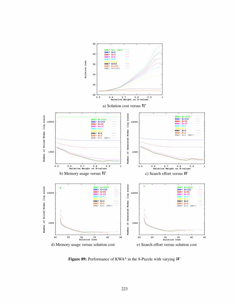
20
25
30
35
40
45
0.5 0.6 0.7 0.8 0.9 1
Solution Cost
Relative Weight on H-values
KWA* K=1 (WA*)KWA* K=2 KWA* K=3 KWA* K=4 KWA* K=5 KWA* K=10 KWA* K=50 KWA* K=100 KWA* K=1000
a) Solution cost versus
1000
10000
0.5 0.6 0.7 0.8 0.9 1
Number of Stored Nodes (log scale)
Relative Weight on H-values
KWA* K=1000 KWA* K=100 KWA* K=50 KWA* K=10 KWA* K=5 KWA* K=4 KWA* K=3 KWA* K=2 KWA* K=1 (WA*)
b) Memory usage versus
1000
10000
0.5 0.6 0.7 0.8 0.9 1
Number of Generated Nodes (log scale)
Relative Weight on H-values
KWA* K=1000 KWA* K=100 KWA* K=50 KWA* K=10 KWA* K=5 KWA* K=4 KWA* K=3 KWA* K=2 KWA* K=1 (WA*)
c) Search effort versus
1000
10000
20 25 30 35 40 45
Number of Stored Nodes (log scale)
Solution Cost
KWA* K=1000 KWA* K=100 KWA* K=50 KWA* K=10 KWA* K=5 KWA* K=4 KWA* K=3 KWA* K=2 KWA* K=1 (WA*)
d) Memory usage versus solution cost
1000
10000
20 25 30 35 40 45
Number of Generated Nodes (log scale)
Solution Cost
KWA* K=1000 KWA* K=100 KWA* K=50 KWA* K=10 KWA* K=5 KWA* K=4 KWA* K=3 KWA* K=2 KWA* K=1 (WA*)
e) Search effort versus solution cost
Figure 89: Performance of KWA* in the 8-Puzzle with varying
223

20
25
30
35
40
45
1 10 100 1000 10000 100000
Solution Cost
Value of K (log scale)
KWA* W=0.99KWA* W=0.95KWA* W=0.90KWA* W=0.86KWA* W=0.80KWA* W=0.75KWA* W=0.67KWA* W=0.60KWA* W=0.56KWA* W=0.50
a) Solution cost versus �
1000
10000
100000
1 10 100 1000 10000 100000
Number of Stored Nodes (log scale)
Value of K (log scale)
KWA* W=0.50KWA* W=0.56KWA* W=0.60KWA* W=0.67KWA* W=0.75KWA* W=0.80KWA* W=0.86KWA* W=0.90KWA* W=0.95KWA* W=0.99
b) Memory usage versus �
1000
10000
100000
1 10 100 1000 10000 100000
Number of Generated Nodes (log scale)
Value of K (log scale)
KWA* W=0.50KWA* W=0.56KWA* W=0.60KWA* W=0.67KWA* W=0.75KWA* W=0.80KWA* W=0.86KWA* W=0.90KWA* W=0.95KWA* W=0.99
c) Search effort versus �
1000
10000
100000
20 25 30 35 40 45
Number of Stored Nodes (log scale)
Solution Cost
KWA* W=0.50KWA* W=0.56KWA* W=0.60KWA* W=0.67KWA* W=0.75KWA* W=0.80KWA* W=0.86KWA* W=0.90KWA* W=0.95KWA* W=0.99
d) Memory usage versus solution cost
1000
10000
100000
20 25 30 35 40 45
Number of Generated Nodes (log scale)
Solution Cost
KWA* W=0.50KWA* W=0.56KWA* W=0.60KWA* W=0.67KWA* W=0.75KWA* W=0.80KWA* W=0.86KWA* W=0.90KWA* W=0.95KWA* W=0.99
e) Search effort versus solution cost
Figure 90: Performance of KWA* in the 8-Puzzle with varying �
224

60
80
100
120
140
0.5 0.6 0.7 0.8 0.9 1
Solution Cost
Relative Weight on H-values
KWA* K=1 (WA*) KWA* K=2 KWA* K=3 KWA* K=4 KWA* K=5 KWA* K=10 KWA* K=50 KWA* K=100 KWA* K=1000 KWA* K=10000
a) Solution cost versus
0.001
0.01
0.1
1
0.5 0.6 0.7 0.8 0.9 1
Time in Seconds (log scale)
Relative Weight on H-values
KWA* K=10000 KWA* K=1000 KWA* K=100 KWA* K=50 KWA* K=10 KWA* K=5 KWA* K=4 KWA* K=3 KWA* K=2 KWA* K=1 (WA*)
b) Runtime versus
1000
10000
100000
1e+06
0.5 0.6 0.7 0.8 0.9 1
Number of Stored Nodes (log scale)
Relative Weight on H-values
KWA* K=10000 KWA* K=1000 KWA* K=100 KWA* K=50 KWA* K=10 KWA* K=5 KWA* K=4 KWA* K=3 KWA* K=2 KWA* K=1 (WA*)
c) Memory usage versus
1000
10000
100000
1e+06
0.5 0.6 0.7 0.8 0.9 1
Number of Generated Nodes (log scale)
Relative Weight on H-values
KWA* K=10000 KWA* K=1000 KWA* K=100 KWA* K=50 KWA* K=10 KWA* K=5 KWA* K=4 KWA* K=3 KWA* K=2 KWA* K=1 (WA*)
d) Search effort versus
1000
10000
100000
1e+06
60 80 100 120 140
Number of Stored Nodes (log scale)
Solution Cost
KWA* K=10000 KWA* K=1000 KWA* K=100 KWA* K=50 KWA* K=10 KWA* K=5 KWA* K=4 KWA* K=3 KWA* K=2 KWA* K=1 (WA*)
e) Memory usage versus solution cost
0.001
0.01
0.1
1
60 80 100 120 140
Time in Seconds (log scale)
Solution Cost
KWA* K=10000 KWA* K=1000 KWA* K=100 KWA* K=50 KWA* K=10 KWA* K=5 KWA* K=4 KWA* K=3 KWA* K=2 KWA* K=1 (WA*)
f) Runtime versus solution cost
Figure 91: Performance of KWA* in the 15-Puzzle with varying
225

60
80
100
120
140
1 10 100 1000 10000 100000
Solution Cost
Value of K (log scale)
KWA* W=0.99KWA* W=0.95KWA* W=0.90KWA* W=0.86KWA* W=0.80KWA* W=0.75KWA* W=0.67
a) Solution cost versus �
0.001
0.01
0.1
1
1 10 100 1000 10000 100000
Time in Seconds (log scale)
Value of K (log scale)
KWA* W=0.67KWA* W=0.75KWA* W=0.80KWA* W=0.86KWA* W=0.90KWA* W=0.95KWA* W=0.99
b) Runtime versus �
1000
10000
100000
1e+06
1 10 100 1000 10000 100000
Number of Stored Nodes (log scale)
Value of K (log scale)
KWA* W=0.67KWA* W=0.75KWA* W=0.80KWA* W=0.86KWA* W=0.90KWA* W=0.95KWA* W=0.99
c) Memory usage versus �
1000
10000
100000
1e+06
1 10 100 1000 10000 100000
Number of Generated Nodes (log scale)
Value of K (log scale)
KWA* W=0.67KWA* W=0.75KWA* W=0.80KWA* W=0.86KWA* W=0.90KWA* W=0.95KWA* W=0.99
d) Search effort versus �
1000
10000
100000
1e+06
60 80 100 120 140
Number of Stored Nodes (log scale)
Solution Cost
KWA* W=0.67KWA* W=0.75KWA* W=0.80KWA* W=0.86KWA* W=0.90KWA* W=0.95KWA* W=0.99
e) Memory usage versus solution cost
0.001
0.01
0.1
1
60 80 100 120 140
Time in Seconds (log scale)
Solution Cost
KWA* W=0.67KWA* W=0.75KWA* W=0.80KWA* W=0.86KWA* W=0.90KWA* W=0.95KWA* W=0.99
f) Runtime versus solution cost
Figure 92: Performance of KWA* in the 15-Puzzle with varying �
226

100
150
200
250
300
350
0.5 0.6 0.7 0.8 0.9 1
Solution Cost
Relative Weight on H-values
KWA* K=1 (WA*) KWA* K=2 KWA* K=3 KWA* K=4 KWA* K=5 KWA* K=10 KWA* K=50 KWA* K=100 KWA* K=1000 KWA* K=10000
a) Solution cost versus
0.01
0.1
1
0.5 0.6 0.7 0.8 0.9 1
Time in Seconds (log scale)
Relative Weight on H-values
KWA* K=10000 KWA* K=1000 KWA* K=100 KWA* K=50 KWA* K=10 KWA* K=5 KWA* K=4 KWA* K=3 KWA* K=2 KWA* K=1 (WA*)
b) Runtime versus
100000
1e+06
0.5 0.6 0.7 0.8 0.9 1
Number of Stored Nodes (log scale)
Relative Weight on H-values
KWA* K=10000 KWA* K=1000 KWA* K=100 KWA* K=50 KWA* K=10 KWA* K=5 KWA* K=4 KWA* K=3 KWA* K=2 KWA* K=1 (WA*)
c) Memory usage versus
100000
1e+06
0.5 0.6 0.7 0.8 0.9 1
Number of Generated Nodes (log scale)
Relative Weight on H-values
KWA* K=10000 KWA* K=1000 KWA* K=100 KWA* K=50 KWA* K=10 KWA* K=5 KWA* K=4 KWA* K=3 KWA* K=2 KWA* K=1 (WA*)
d) Search effort versus
100000
1e+06
100 150 200 250 300 350
Number of Stored Nodes (log scale)
Solution Cost
KWA* K=10000 KWA* K=1000 KWA* K=100 KWA* K=50 KWA* K=10 KWA* K=5 KWA* K=4 KWA* K=3 KWA* K=2 KWA* K=1 (WA*)
e) Memory usage versus solution cost
0.01
0.1
1
100 150 200 250 300 350
Time in Seconds (log scale)
Solution Cost
KWA* K=10000 KWA* K=1000 KWA* K=100 KWA* K=50 KWA* K=10 KWA* K=5 KWA* K=4 KWA* K=3 KWA* K=2 KWA* K=1 (WA*)
f) Runtime versus solution cost
Figure 93: Performance of KWA* in the 24-Puzzle with varying
227

100
150
200
250
300
350
1 10 100 1000 10000 100000
Solution Cost
Value of K (log scale)
KWA* W=0.99KWA* W=0.95KWA* W=0.90KWA* W=0.86KWA* W=0.80KWA* W=0.75
a) Solution cost versus �
0.01
0.1
1
1 10 100 1000 10000 100000
Time in Seconds (log scale)
Value of K (log scale)
KWA* W=0.75KWA* W=0.80KWA* W=0.86KWA* W=0.90KWA* W=0.95KWA* W=0.99
b) Runtime versus �
100000
1e+06
1 10 100 1000 10000 100000
Number of Stored Nodes (log scale)
Value of K (log scale)
KWA* W=0.75KWA* W=0.80KWA* W=0.86KWA* W=0.90KWA* W=0.95KWA* W=0.99
c) Memory usage versus �
100000
1e+06
1 10 100 1000 10000 100000
Number of Generated Nodes (log scale)
Value of K (log scale)
KWA* W=0.75KWA* W=0.80KWA* W=0.86KWA* W=0.90KWA* W=0.95KWA* W=0.99
d) Search effort versus �
100000
1e+06
100 150 200 250 300 350
Number of Stored Nodes (log scale)
Solution Cost
KWA* W=0.75KWA* W=0.80KWA* W=0.86KWA* W=0.90KWA* W=0.95KWA* W=0.99
e) Memory usage versus solution cost
0.01
0.1
1
100 150 200 250 300 350
Time in Seconds (log scale)
Solution Cost
KWA* W=0.75KWA* W=0.80KWA* W=0.86KWA* W=0.90KWA* W=0.95KWA* W=0.99
f) Runtime versus solution cost
Figure 94: Performance of KWA* in the 24-Puzzle with varying �
228

B.2 Empirical evaluation of MSC-WA* in the]
-Puzzle
229
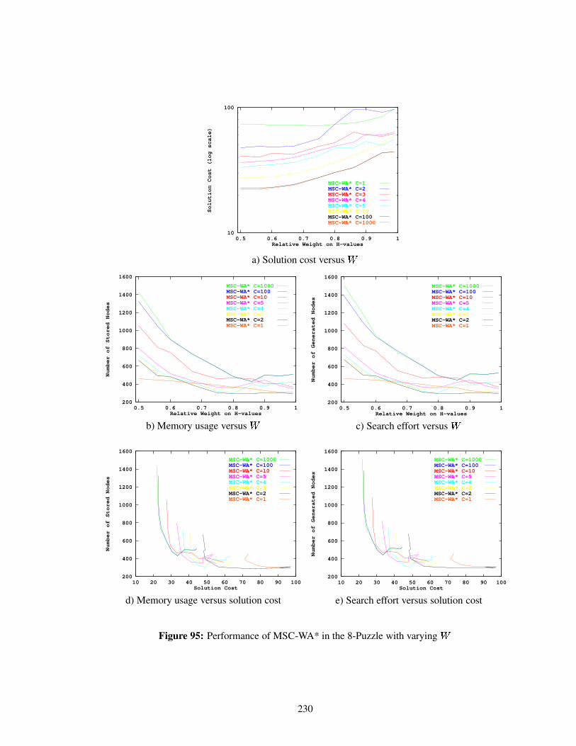
10
100
0.5 0.6 0.7 0.8 0.9 1
Solution Cost (log scale)
Relative Weight on H-values
MSC-WA* C=1 MSC-WA* C=2 MSC-WA* C=3 MSC-WA* C=4 MSC-WA* C=5 MSC-WA* C=10 MSC-WA* C=100 MSC-WA* C=1000
a) Solution cost versus
200
400
600
800
1000
1200
1400
1600
0.5 0.6 0.7 0.8 0.9 1
Number of Stored Nodes
Relative Weight on H-values
MSC-WA* C=1000MSC-WA* C=100 MSC-WA* C=10 MSC-WA* C=5 MSC-WA* C=4 MSC-WA* C=3 MSC-WA* C=2 MSC-WA* C=1
b) Memory usage versus
200
400
600
800
1000
1200
1400
1600
0.5 0.6 0.7 0.8 0.9 1
Number of Generated Nodes
Relative Weight on H-values
MSC-WA* C=1000MSC-WA* C=100 MSC-WA* C=10 MSC-WA* C=5 MSC-WA* C=4 MSC-WA* C=3 MSC-WA* C=2 MSC-WA* C=1
c) Search effort versus
200
400
600
800
1000
1200
1400
1600
10 20 30 40 50 60 70 80 90 100
Number of Stored Nodes
Solution Cost
MSC-WA* C=1000MSC-WA* C=100 MSC-WA* C=10 MSC-WA* C=5 MSC-WA* C=4 MSC-WA* C=3 MSC-WA* C=2 MSC-WA* C=1
d) Memory usage versus solution cost
200
400
600
800
1000
1200
1400
1600
10 20 30 40 50 60 70 80 90 100
Number of Generated Nodes
Solution Cost
MSC-WA* C=1000MSC-WA* C=100 MSC-WA* C=10 MSC-WA* C=5 MSC-WA* C=4 MSC-WA* C=3 MSC-WA* C=2 MSC-WA* C=1
e) Search effort versus solution cost
Figure 95: Performance of MSC-WA* in the 8-Puzzle with varying
230

10
20
30
40
50
60
70
80
90
100
1 10 100 1000 10000 100000
Solution Cost
Value of C (log scale)
MSC-WA* W=0.99MSC-WA* W=0.95MSC-WA* W=0.90MSC-WA* W=0.86MSC-WA* W=0.80MSC-WA* W=0.75MSC-WA* W=0.67MSC-WA* W=0.60MSC-WA* W=0.56MSC-WA* W=0.50
a) Solution cost versus �
200
400
600
800
1000
1200
1400
1600
1 10 100 1000 10000 100000
Number of Stored Nodes
Value of C (log scale)
MSC-WA* W=0.50MSC-WA* W=0.56MSC-WA* W=0.60MSC-WA* W=0.67MSC-WA* W=0.75MSC-WA* W=0.80MSC-WA* W=0.86MSC-WA* W=0.90MSC-WA* W=0.95MSC-WA* W=0.99
b) Memory usage versus �
200
400
600
800
1000
1200
1400
1600
1 10 100 1000 10000 100000
Number of Generated Nodes
Value of C (log scale)
MSC-WA* W=0.50MSC-WA* W=0.56MSC-WA* W=0.60MSC-WA* W=0.67MSC-WA* W=0.75MSC-WA* W=0.80MSC-WA* W=0.86MSC-WA* W=0.90MSC-WA* W=0.95MSC-WA* W=0.99
c) Search effort versus �
200
400
600
800
1000
1200
1400
1600
10 20 30 40 50 60 70 80 90 100
Number of Stored Nodes
Solution Cost
MSC-WA* W=0.50MSC-WA* W=0.56MSC-WA* W=0.60MSC-WA* W=0.67MSC-WA* W=0.75MSC-WA* W=0.80MSC-WA* W=0.86MSC-WA* W=0.90MSC-WA* W=0.95MSC-WA* W=0.99
d) Memory usage versus solution cost
200
400
600
800
1000
1200
1400
1600
10 20 30 40 50 60 70 80 90 100
Number of Generated Nodes
Solution Cost
MSC-WA* W=0.50MSC-WA* W=0.56MSC-WA* W=0.60MSC-WA* W=0.67MSC-WA* W=0.75MSC-WA* W=0.80MSC-WA* W=0.86MSC-WA* W=0.90MSC-WA* W=0.95MSC-WA* W=0.99
e) Search effort versus solution cost
Figure 96: Performance of MSC-WA* in the 8-Puzzle with varying �
231
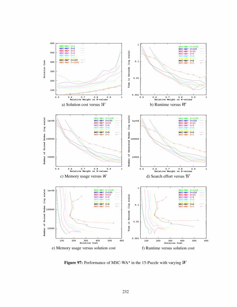
100
200
300
400
500
600
0.5 0.6 0.7 0.8 0.9 1
Solution Cost
Relative Weight on H-values
MSC-WA* C=1 MSC-WA* C=2 MSC-WA* C=3 MSC-WA* C=4 MSC-WA* C=5 MSC-WA* C=10 MSC-WA* C=100 MSC-WA* C=1000
a) Solution cost versus
0.001
0.01
0.1
1
0.5 0.6 0.7 0.8 0.9 1
Time in Seconds (log scale)
Relative Weight on H-values
MSC-WA* C=1000MSC-WA* C=100 MSC-WA* C=10 MSC-WA* C=5 MSC-WA* C=4 MSC-WA* C=3 MSC-WA* C=2 MSC-WA* C=1
b) Runtime versus
10000
100000
1e+06
0.5 0.6 0.7 0.8 0.9 1
Number of Stored Nodes (log scale)
Relative Weight on H-values
MSC-WA* C=1000MSC-WA* C=100 MSC-WA* C=10 MSC-WA* C=5 MSC-WA* C=4 MSC-WA* C=3 MSC-WA* C=2 MSC-WA* C=1
c) Memory usage versus
10000
100000
1e+06
0.5 0.6 0.7 0.8 0.9 1
Number of Generated Nodes (log scale)
Relative Weight on H-values
MSC-WA* C=1000MSC-WA* C=100 MSC-WA* C=10 MSC-WA* C=5 MSC-WA* C=4 MSC-WA* C=3 MSC-WA* C=2 MSC-WA* C=1
d) Search effort versus
10000
100000
1e+06
100 200 300 400 500 600
Number of Stored Nodes (log scale)
Solution Cost
MSC-WA* C=1000MSC-WA* C=100 MSC-WA* C=10 MSC-WA* C=5 MSC-WA* C=4 MSC-WA* C=3 MSC-WA* C=2 MSC-WA* C=1
e) Memory usage versus solution cost
0.001
0.01
0.1
1
100 200 300 400 500 600
Time in Seconds (log scale)
Solution Cost
MSC-WA* C=1000MSC-WA* C=100 MSC-WA* C=10 MSC-WA* C=5 MSC-WA* C=4 MSC-WA* C=3 MSC-WA* C=2 MSC-WA* C=1
f) Runtime versus solution cost
Figure 97: Performance of MSC-WA* in the 15-Puzzle with varying
232
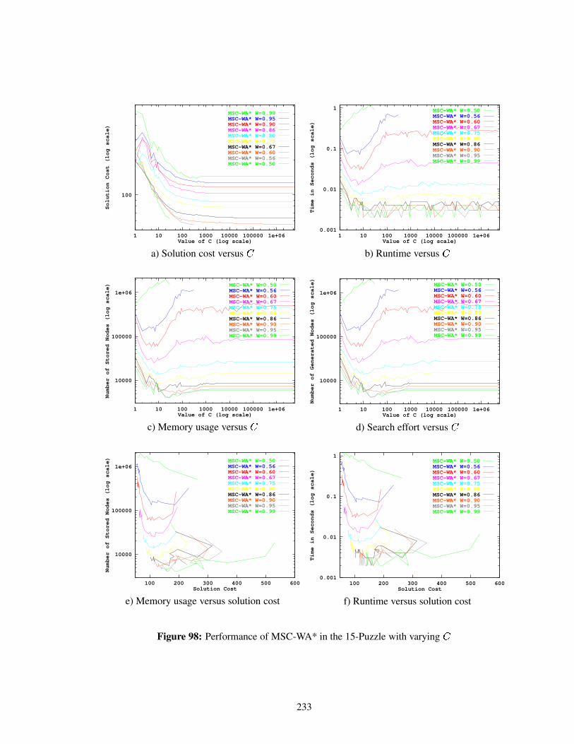
100
1 10 100 1000 10000 100000 1e+06
Solution Cost (log scale)
Value of C (log scale)
MSC-WA* W=0.99MSC-WA* W=0.95MSC-WA* W=0.90MSC-WA* W=0.86MSC-WA* W=0.80MSC-WA* W=0.75MSC-WA* W=0.67MSC-WA* W=0.60MSC-WA* W=0.56MSC-WA* W=0.50
a) Solution cost versus �
0.001
0.01
0.1
1
1 10 100 1000 10000 100000 1e+06
Time in Seconds (log scale)
Value of C (log scale)
MSC-WA* W=0.50MSC-WA* W=0.56MSC-WA* W=0.60MSC-WA* W=0.67MSC-WA* W=0.75MSC-WA* W=0.80MSC-WA* W=0.86MSC-WA* W=0.90MSC-WA* W=0.95MSC-WA* W=0.99
b) Runtime versus �
10000
100000
1e+06
1 10 100 1000 10000 100000 1e+06
Number of Stored Nodes (log scale)
Value of C (log scale)
MSC-WA* W=0.50MSC-WA* W=0.56MSC-WA* W=0.60MSC-WA* W=0.67MSC-WA* W=0.75MSC-WA* W=0.80MSC-WA* W=0.86MSC-WA* W=0.90MSC-WA* W=0.95MSC-WA* W=0.99
c) Memory usage versus �
10000
100000
1e+06
1 10 100 1000 10000 100000 1e+06
Number of Generated Nodes (log scale)
Value of C (log scale)
MSC-WA* W=0.50MSC-WA* W=0.56MSC-WA* W=0.60MSC-WA* W=0.67MSC-WA* W=0.75MSC-WA* W=0.80MSC-WA* W=0.86MSC-WA* W=0.90MSC-WA* W=0.95MSC-WA* W=0.99
d) Search effort versus �
10000
100000
1e+06
100 200 300 400 500 600
Number of Stored Nodes (log scale)
Solution Cost
MSC-WA* W=0.50MSC-WA* W=0.56MSC-WA* W=0.60MSC-WA* W=0.67MSC-WA* W=0.75MSC-WA* W=0.80MSC-WA* W=0.86MSC-WA* W=0.90MSC-WA* W=0.95MSC-WA* W=0.99
e) Memory usage versus solution cost
0.001
0.01
0.1
1
100 200 300 400 500 600
Time in Seconds (log scale)
Solution Cost
MSC-WA* W=0.50MSC-WA* W=0.56MSC-WA* W=0.60MSC-WA* W=0.67MSC-WA* W=0.75MSC-WA* W=0.80MSC-WA* W=0.86MSC-WA* W=0.90MSC-WA* W=0.95MSC-WA* W=0.99
f) Runtime versus solution cost
Figure 98: Performance of MSC-WA* in the 15-Puzzle with varying �
233

200
400
600
800
1000
1200
0.5 0.6 0.7 0.8 0.9 1
Solution Cost
Relative Weight on H-values
MSC-WA* C=1 MSC-WA* C=2 MSC-WA* C=3 MSC-WA* C=4 MSC-WA* C=5 MSC-WA* C=10 MSC-WA* C=100 MSC-WA* C=1000
a) Solution cost versus
0.01
0.1
1
0.5 0.6 0.7 0.8 0.9 1
Time in Seconds (log scale)
Relative Weight on H-values
MSC-WA* C=1 MSC-WA* C=2 MSC-WA* C=3 MSC-WA* C=4 MSC-WA* C=5 MSC-WA* C=10 MSC-WA* C=100 MSC-WA* C=1000
b) Runtime versus
100000
1e+06
0.5 0.6 0.7 0.8 0.9 1
Number of Stored Nodes (log scale)
Relative Weight on H-values
MSC-WA* C=1 MSC-WA* C=2 MSC-WA* C=3 MSC-WA* C=4 MSC-WA* C=5 MSC-WA* C=10 MSC-WA* C=100 MSC-WA* C=1000
c) Memory usage versus
100000
1e+06
0.5 0.6 0.7 0.8 0.9 1
Number of Generated Nodes (log scale)
Relative Weight on H-values
MSC-WA* C=1 MSC-WA* C=2 MSC-WA* C=3 MSC-WA* C=4 MSC-WA* C=5 MSC-WA* C=10 MSC-WA* C=100 MSC-WA* C=1000
d) Search effort versus
100000
1e+06
200 400 600 800 1000 1200
Number of Stored Nodes (log scale)
Solution Cost
MSC-WA* C=1 MSC-WA* C=2 MSC-WA* C=3 MSC-WA* C=4 MSC-WA* C=5 MSC-WA* C=10 MSC-WA* C=100 MSC-WA* C=1000
e) Memory usage versus solution cost
0.01
0.1
1
200 400 600 800 1000 1200
Time in Seconds (log scale)
Solution Cost
MSC-WA* C=1 MSC-WA* C=2 MSC-WA* C=3 MSC-WA* C=4 MSC-WA* C=5 MSC-WA* C=10 MSC-WA* C=100 MSC-WA* C=1000
f) Runtime versus solution cost
Figure 99: Performance of MSC-WA* in the 24-Puzzle with varying
234

200
400
600
800
1000
1200
1 10 100 1000 10000 100000 1e+06
Solution Cost
Value of C (log scale)
MSC-WA* W=0.99MSC-WA* W=0.95MSC-WA* W=0.90MSC-WA* W=0.86MSC-WA* W=0.80MSC-WA* W=0.75
a) Solution cost versus �
0.01
0.1
1
1 10 100 1000 10000 100000 1e+06
Time in Seconds (log scale)
Value of C (log scale)
MSC-WA* W=0.75MSC-WA* W=0.80MSC-WA* W=0.86MSC-WA* W=0.90MSC-WA* W=0.95MSC-WA* W=0.99
b) Runtime versus �
100000
1e+06
1 10 100 1000 10000 100000 1e+06
Number of Stored Nodes (log scale)
Value of C (log scale)
MSC-WA* W=0.75MSC-WA* W=0.80MSC-WA* W=0.86MSC-WA* W=0.90MSC-WA* W=0.95MSC-WA* W=0.99
c) Memory usage versus �
100000
1e+06
1 10 100 1000 10000 100000 1e+06
Number of Generated Nodes (log scale)
Value of C (log scale)
MSC-WA* W=0.75MSC-WA* W=0.80MSC-WA* W=0.86MSC-WA* W=0.90MSC-WA* W=0.95MSC-WA* W=0.99
d) Search effort versus �
100000
1e+06
200 400 600 800 1000 1200
Number of Stored Nodes (log scale)
Solution Cost
MSC-WA* W=0.75MSC-WA* W=0.80MSC-WA* W=0.86MSC-WA* W=0.90MSC-WA* W=0.95MSC-WA* W=0.99
e) Memory usage versus solution cost
0.01
0.1
1
200 400 600 800 1000 1200
Time in Seconds (log scale)
Solution Cost
MSC-WA* W=0.75MSC-WA* W=0.80MSC-WA* W=0.86MSC-WA* W=0.90MSC-WA* W=0.95MSC-WA* W=0.99
f) Runtime versus solution cost
Figure 100: Performance of MSC-WA* in the 24-Puzzle with varying �
235

B.3 Empirical evaluation of MSC-KWA* in the]
-Puzzle
236

10
20
30
40
50
60
70
80
90
100
0.5 0.6 0.7 0.8 0.9 1
Solution Cost
Relative Weight on H-values
MSC-KWA* K=1 MSC-KWA* K=2 MSC-KWA* K=3 MSC-KWA* K=4 MSC-KWA* K=5 MSC-KWA* K=10 MSC-KWA* K=100 MSC-KWA* K=50000
a) Solution cost versus
100
1000
10000
100000
0.5 0.6 0.7 0.8 0.9 1
Number of Stored Nodes (log scale)
Relative Weight on H-values
MSC-KWA* K=50000MSC-KWA* K=100 MSC-KWA* K=10 MSC-KWA* K=5 MSC-KWA* K=4 MSC-KWA* K=3 MSC-KWA* K=2 MSC-KWA* K=1
b) Memory usage versus
100
1000
10000
100000
0.5 0.6 0.7 0.8 0.9 1
Number of Generated Nodes (log scale)
Relative Weight on H-values
MSC-KWA* K=50000MSC-KWA* K=100 MSC-KWA* K=10 MSC-KWA* K=5 MSC-KWA* K=4 MSC-KWA* K=3 MSC-KWA* K=2 MSC-KWA* K=1
c) Search effort versus
100
1000
10000
100000
10 20 30 40 50 60 70 80 90 100
Number of Stored Nodes (log scale)
Solution Cost
MSC-KWA* K=50000MSC-KWA* K=100 MSC-KWA* K=10 MSC-KWA* K=5 MSC-KWA* K=4 MSC-KWA* K=3 MSC-KWA* K=2 MSC-KWA* K=1
d) Memory usage versus solution cost
100
1000
10000
100000
10 20 30 40 50 60 70 80 90 100
Number of Generated Nodes (log scale)
Solution Cost
MSC-KWA* K=50000MSC-KWA* K=100 MSC-KWA* K=10 MSC-KWA* K=5 MSC-KWA* K=4 MSC-KWA* K=3 MSC-KWA* K=2 MSC-KWA* K=1
e) Search effort versus solution cost
Figure 101: Performance of MSC-KWA* in the 8-Puzzle with varying
237
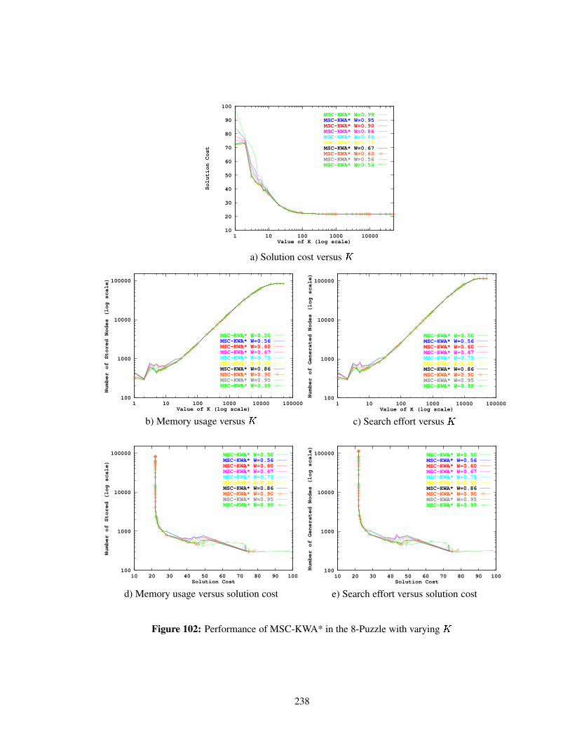
10
20
30
40
50
60
70
80
90
100
1 10 100 1000 10000
Solution Cost
Value of K (log scale)
MSC-KWA* W=0.99MSC-KWA* W=0.95MSC-KWA* W=0.90MSC-KWA* W=0.86MSC-KWA* W=0.80MSC-KWA* W=0.75MSC-KWA* W=0.67MSC-KWA* W=0.60MSC-KWA* W=0.56MSC-KWA* W=0.50
a) Solution cost versus �
100
1000
10000
100000
1 10 100 1000 10000 100000
Number of Stored Nodes (log scale)
Value of K (log scale)
MSC-KWA* W=0.50MSC-KWA* W=0.56MSC-KWA* W=0.60MSC-KWA* W=0.67MSC-KWA* W=0.75MSC-KWA* W=0.80MSC-KWA* W=0.86MSC-KWA* W=0.90MSC-KWA* W=0.95MSC-KWA* W=0.99
b) Memory usage versus �
100
1000
10000
100000
1 10 100 1000 10000 100000
Number of Generated Nodes (log scale)
Value of K (log scale)
MSC-KWA* W=0.50MSC-KWA* W=0.56MSC-KWA* W=0.60MSC-KWA* W=0.67MSC-KWA* W=0.75MSC-KWA* W=0.80MSC-KWA* W=0.86MSC-KWA* W=0.90MSC-KWA* W=0.95MSC-KWA* W=0.99
c) Search effort versus �
100
1000
10000
100000
10 20 30 40 50 60 70 80 90 100
Number of Stored (log scale)
Solution Cost
MSC-KWA* W=0.50MSC-KWA* W=0.56MSC-KWA* W=0.60MSC-KWA* W=0.67MSC-KWA* W=0.75MSC-KWA* W=0.80MSC-KWA* W=0.86MSC-KWA* W=0.90MSC-KWA* W=0.95MSC-KWA* W=0.99
d) Memory usage versus solution cost
100
1000
10000
100000
10 20 30 40 50 60 70 80 90 100
Number of Generated Nodes (log scale)
Solution Cost
MSC-KWA* W=0.50MSC-KWA* W=0.56MSC-KWA* W=0.60MSC-KWA* W=0.67MSC-KWA* W=0.75MSC-KWA* W=0.80MSC-KWA* W=0.86MSC-KWA* W=0.90MSC-KWA* W=0.95MSC-KWA* W=0.99
e) Search effort versus solution cost
Figure 102: Performance of MSC-KWA* in the 8-Puzzle with varying �
238

10
100
1000
0.5 0.6 0.7 0.8 0.9 1
Solution Cost (log scale)
Relative Weight on H-values
MSC-KWA* K=1 MSC-KWA* K=2 MSC-KWA* K=3 MSC-KWA* K=4 MSC-KWA* K=5 MSC-KWA* K=10 MSC-KWA* K=100 MSC-KWA* K=50000
a) Solution cost versus
0.001
0.01
0.1
1
0.5 0.6 0.7 0.8 0.9 1
Time in Seconds (log scale)
Relative Weight on H-values
MSC-KWA* K=50000MSC-KWA* K=100 MSC-KWA* K=10 MSC-KWA* K=5 MSC-KWA* K=4 MSC-KWA* K=3 MSC-KWA* K=2 MSC-KWA* K=1
b) Runtime versus
1000
10000
100000
1e+06
0.5 0.6 0.7 0.8 0.9 1
Number of Stored Nodes (log scale)
Relative Weight on H-values
MSC-KWA* K=50000MSC-KWA* K=100 MSC-KWA* K=10 MSC-KWA* K=5 MSC-KWA* K=4 MSC-KWA* K=3 MSC-KWA* K=2 MSC-KWA* K=1
c) Memory usage versus
1000
10000
100000
1e+06
0.5 0.6 0.7 0.8 0.9 1
Number of Generated Nodes (log scale)
Relative Weight on H-values
MSC-KWA* K=50000MSC-KWA* K=100 MSC-KWA* K=10 MSC-KWA* K=5 MSC-KWA* K=4 MSC-KWA* K=3 MSC-KWA* K=2 MSC-KWA* K=1
d) Search effort versus
1000
10000
100000
1e+06
200 400 600 800 1000 1200
Number of Stored Nodes (log scale)
Solution Cost
MSC-KWA* K=50000MSC-KWA* K=100 MSC-KWA* K=10 MSC-KWA* K=5 MSC-KWA* K=4 MSC-KWA* K=3 MSC-KWA* K=2 MSC-KWA* K=1
e) Memory usage versus solution cost
0.001
0.01
0.1
1
200 400 600 800 1000 1200
Time in Seconds (log scale)
Solution Cost
MSC-KWA* K=50000MSC-KWA* K=100 MSC-KWA* K=10 MSC-KWA* K=5 MSC-KWA* K=4 MSC-KWA* K=3 MSC-KWA* K=2 MSC-KWA* K=1
f) Runtime versus solution cost
Figure 103: Performance of MSC-KWA* in the 15-Puzzle with varying
239

10
100
1000
1 10 100 1000 10000
Solution Cost (log scale)
Value of K (log scale)
MSC-KWA* W=0.99MSC-KWA* W=0.95MSC-KWA* W=0.90MSC-KWA* W=0.86MSC-KWA* W=0.80MSC-KWA* W=0.75MSC-KWA* W=0.67MSC-KWA* W=0.60MSC-KWA* W=0.56MSC-KWA* W=0.50
a) Solution cost versus �
0.001
0.01
0.1
1
1 10 100 1000 10000
Time in Seconds (log scale)
Value of K (log scale)
MSC-KWA* W=0.50MSC-KWA* W=0.56MSC-KWA* W=0.60MSC-KWA* W=0.67MSC-KWA* W=0.75MSC-KWA* W=0.80MSC-KWA* W=0.86MSC-KWA* W=0.90MSC-KWA* W=0.95MSC-KWA* W=0.99
b) Runtime versus �
1000
10000
100000
1e+06
1 10 100 1000 10000
Number of Stored Nodes (log scale)
Value of K (log scale)
MSC-KWA* W=0.50MSC-KWA* W=0.56MSC-KWA* W=0.60MSC-KWA* W=0.67MSC-KWA* W=0.75MSC-KWA* W=0.80MSC-KWA* W=0.86MSC-KWA* W=0.90MSC-KWA* W=0.95MSC-KWA* W=0.99
c) Memory usage versus �
1000
10000
100000
1e+06
1 10 100 1000 10000
Number of Generated Nodes (log scale)
Value of K (log scale)
MSC-KWA* W=0.50MSC-KWA* W=0.56MSC-KWA* W=0.60MSC-KWA* W=0.67MSC-KWA* W=0.75MSC-KWA* W=0.80MSC-KWA* W=0.86MSC-KWA* W=0.90MSC-KWA* W=0.95MSC-KWA* W=0.99
d) Search effort versus �
1000
10000
100000
1e+06
200 400 600 800 1000 1200
Number of Stored Nodes (log scale)
Solution Cost
MSC-KWA* W=0.50MSC-KWA* W=0.56MSC-KWA* W=0.60MSC-KWA* W=0.67MSC-KWA* W=0.75MSC-KWA* W=0.80MSC-KWA* W=0.86MSC-KWA* W=0.90MSC-KWA* W=0.95MSC-KWA* W=0.99
e) Memory usage versus solution cost
0.001
0.01
0.1
1
200 400 600 800 1000 1200
Time in Seconds (log scale)
Solution Cost
MSC-KWA* W=0.50MSC-KWA* W=0.56MSC-KWA* W=0.60MSC-KWA* W=0.67MSC-KWA* W=0.75MSC-KWA* W=0.80MSC-KWA* W=0.86MSC-KWA* W=0.90MSC-KWA* W=0.95MSC-KWA* W=0.99
f) Runtime versus solution cost
Figure 104: Performance of MSC-KWA* in the 15-Puzzle with varying �
240
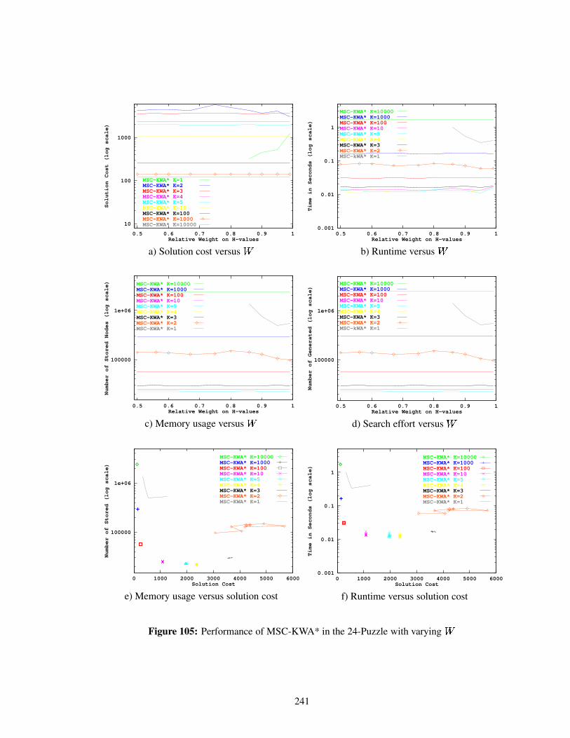
10
100
1000
0.5 0.6 0.7 0.8 0.9 1
Solution Cost (log scale)
Relative Weight on H-values
MSC-KWA* K=1 MSC-KWA* K=2 MSC-KWA* K=3 MSC-KWA* K=4 MSC-KWA* K=5 MSC-KWA* K=10 MSC-KWA* K=100 MSC-KWA* K=1000 MSC-KWA* K=10000
a) Solution cost versus
0.001
0.01
0.1
1
0.5 0.6 0.7 0.8 0.9 1
Time in Seconds (log scale)
Relative Weight on H-values
MSC-KWA* K=10000MSC-KWA* K=1000 MSC-KWA* K=100 MSC-KWA* K=10 MSC-KWA* K=5 MSC-KWA* K=4 MSC-KWA* K=3 MSC-KWA* K=2 MSC-kWA* K=1
b) Runtime versus
100000
1e+06
0.5 0.6 0.7 0.8 0.9 1
Number of Stored Nodes (log scale)
Relative Weight on H-values
MSC-KWA* K=10000MSC-KWA* K=1000 MSC-KWA* K=100 MSC-KWA* K=10 MSC-KWA* K=5 MSC-KWA* K=4 MSC-KWA* K=3 MSC-KWA* K=2 MSC-KWA* K=1
c) Memory usage versus
100000
1e+06
0.5 0.6 0.7 0.8 0.9 1
Number of Generated (log scale)
Relative Weight on H-values
MSC-KWA* K=10000MSC-KWA* K=1000 MSC-KWA* K=100 MSC-KWA* K=10 MSC-KWA* K=5 MSC-KWA* K=4 MSC-KWA* K=3 MSC-KWA* K=2 MSC-kWA* K=1
d) Search effort versus
100000
1e+06
0 1000 2000 3000 4000 5000 6000
Number of Stored (log scale)
Solution Cost
MSC-KWA* K=10000MSC-KWA* K=1000 MSC-KWA* K=100 MSC-KWA* K=10 MSC-KWA* K=5 MSC-KWA* K=4 MSC-KWA* K=3 MSC-KWA* K=2 MSC-KWA* K=1
e) Memory usage versus solution cost
0.001
0.01
0.1
1
0 1000 2000 3000 4000 5000 6000
Time in Seconds (log scale)
Solution Cost
MSC-KWA* K=10000MSC-KWA* K=1000 MSC-KWA* K=100 MSC-KWA* K=10 MSC-KWA* K=5 MSC-KWA* K=4 MSC-KWA* K=3 MSC-KWA* K=2 MSC-KWA* K=1
f) Runtime versus solution cost
Figure 105: Performance of MSC-KWA* in the 24-Puzzle with varying
241

0
1000
2000
3000
4000
5000
6000
1 10 100 1000 10000
Solution Cost
Value of K (log scale)
MSC-KWA* W=0.99MSC-KWA* W=0.95MSC-KWA* W=0.90MSC-KWA* W=0.86MSC-KWA* W=0.80MSC-KWA* W=0.75MSC-KWA* W=0.67MSC-KWA* W=0.60MSC-KWA* W=0.56MSC-KWA* W=0.50
a) Solution cost versus �
0.001
0.01
0.1
1
1 10 100 1000 10000
Time in Seconds (log scale)
Value of K (log scale)
MSC-KWA* W=0.50MSC-KWA* W=0.56MSC-KWA* W=0.60MSC-KWA* W=0.67MSC-KWA* W=0.75MSC-KWA* W=0.80MSC-KWA* W=0.86MSC-KWA* W=0.90MSC-KWA* W=0.95MSC-KWA* W=0.99
b) Runtime versus �
100000
1e+06
1 10 100 1000 10000
Number of Stored Nodes (log scale)
Value of K (log scale)
MSC-KWA* W=0.50MSC-KWA* W=0.56MSC-KWA* W=0.60MSC-KWA* W=0.67MSC-KWA* W=0.75MSC-KWA* W=0.80MSC-KWA* W=0.86MSC-KWA* W=0.90MSC-KWA* W=0.95MSC-KWA* W=0.99
c) Memory usage versus �
100000
1e+06
1 10 100 1000 10000
Number of Generated Nodes (log scale)
Value of K (log scale)
MSC-KWA* W=0.50MSC-KWA* W=0.56MSC-KWA* W=0.60MSC-KWA* W=0.67MSC-KWA* W=0.75MSC-KWA* W=0.80MSC-KWA* W=0.86MSC-KWA* W=0.90MSC-KWA* W=0.95MSC-KWA* W=0.99
d) Search effort versus �
100000
1e+06
0 1000 2000 3000 4000 5000 6000
Number of Stored Nodes (log scale)
Solution Cost
MSC-KWA* W=0.50MSC-KWA* W=0.56MSC-KWA* W=0.60MSC-KWA* W=0.67MSC-KWA* W=0.75MSC-KWA* W=0.80MSC-KWA* W=0.86MSC-KWA* W=0.90MSC-KWA* W=0.95MSC-KWA* W=0.99
e) Memory usage versus solution cost
0.01
0.1
1
0 1000 2000 3000 4000 5000 6000
Time in Seconds (log scale)
Solution Cost
MSC-KWA* W=0.50MSC-KWA* W=0.56MSC-KWA* W=0.60MSC-KWA* W=0.67MSC-KWA* W=0.75MSC-KWA* W=0.80MSC-KWA* W=0.86MSC-KWA* W=0.90MSC-KWA* W=0.95MSC-KWA* W=0.99
f) Runtime versus solution cost
Figure 106: Performance of MSC-KWA* in the 24-Puzzle with varying �
242

100
1000
10000
0.5 0.6 0.7 0.8 0.9 1
Solution Cost (log scale)
Relative Weight on H-values
MSC-KWA* K=2 MSC-KWA* K=3 MSC-KWA* K=4 MSC-KWA* K=5 MSC-KWA* K=10 MSC-KWA* K=100 MSC-KWA* K=1000 MSC-KWA* K=7000
a) Solution cost versus
0.01
0.1
1
0.5 0.6 0.7 0.8 0.9 1
Time in Seconds(log scale)
Relative Weight on H-values
MSC-KWA* K=7000MSC-KWA* K=1000MSC-KWA* K=100 MSC-KWA* K=10 MSC-KWA* K=5 MSC-KWA* K=4 MSC-KWA* K=3 MSC-KWA* K=2
b) Runtime versus
100000
1e+06
0.5 0.6 0.7 0.8 0.9 1
Number of Stored Nodes (log scale)
Relative Weight on H-values
MSC-KWA* K=7000MSC-KWA* K=1000MSC-KWA* K=100 MSC-KWA* K=10 MSC-KWA* K=5 MSC-KWA* K=4 MSC-KWA* K=3 MSC-KWA* K=2
c) Memory usage versus
100000
1e+06
0.5 0.6 0.7 0.8 0.9 1
Number of Generated Nodes (log scale)
Relative Weight on H-values
MSC-KWA* K=7000MSC-KWA* K=1000MSC-KWA* K=100 MSC-KWA* K=10 MSC-KWA* K=5 MSC-KWA* K=4 MSC-KWA* K=3 MSC-KWA* K=2
d) Search effort versus
100000
1e+06
100 1000 10000
Number of Stored Nodes (log scale)
Solution Cost (log scale)
MSC-KWA* K=7000MSC-KWA* K=1000MSC-KWA* K=100 MSC-KWA* K=10 MSC-KWA* K=5 MSC-KWA* K=4 MSC-KWA* K=3 MSC-KWA* K=2
e) Memory usage versus solution cost
0.01
0.1
1
100 1000 10000
Time in Seconds (log scale)
Solution Cost (log scale)
MSC-KWA* K=7000MSC-KWA* K=1000MSC-KWA* K=100 MSC-KWA* K=10 MSC-KWA* K=5 MSC-KWA* K=4 MSC-KWA* K=3 MSC-KWA* K=2
f) Runtime versus solution cost
Figure 107: Performance of MSC-KWA* in the 35-Puzzle with varying
243

100
1000
10000
1 10 100 1000
Solution Cost (log scale)
Value of K (log scale)
MSC-KWA* W=0.99MSC-KWA* W=0.95MSC-KWA* W=0.90MSC-KWA* W=0.86MSC-KWA* W=0.80MSC-KWA* W=0.75MSC-KWA* W=0.67MSC-KWA* W=0.60MSC-KWA* W=0.56MSC-KWA* W=0.50
a) Solution cost versus �
0.01
0.1
1
1 10 100 1000
Time in Seconds (log scale)
Value of K (log scale)
MSC-KWA* W=0.50MSC-KWA* W=0.56MSC-KWA* W=0.60MSC-KWA* W=0.67MSC-KWA* W=0.75MSC-KWA* W=0.80MSC-KWA* W=0.86MSC-KWA* W=0.90MSC-KWA* W=0.95MSC-KWA* W=0.99
b) Runtime versus �
100000
1e+06
1 10 100 1000
Number of Stored Nodes (log scale)
Value of K (log scale)
MSC-KWA* W=0.50MSC-KWA* W=0.56MSC-KWA* W=0.60MSC-KWA* W=0.67MSC-KWA* W=0.75MSC-KWA* W=0.80MSC-KWA* W=0.86MSC-KWA* W=0.90MSC-KWA* W=0.95MSC-KWA* W=0.99
c) Memory usage versus �
100000
1e+06
1 10 100 1000
Number of Generated Nodes (log scale)
Value of K (log scale)
MSC-KWA* W=0.50MSC-KWA* W=0.56MSC-KWA* W=0.60MSC-KWA* W=0.67MSC-KWA* W=0.75MSC-KWA* W=0.80MSC-KWA* W=0.86MSC-KWA* W=0.90MSC-KWA* W=0.95MSC-KWA* W=0.99
d) Search effort versus �
100000
1e+06
100 1000 10000
Number of Stored Nodes (log scale)
Solution Cost (log scale)
MSC-KWA* W=0.50MSC-KWA* W=0.56MSC-KWA* W=0.60MSC-KWA* W=0.67MSC-KWA* W=0.75MSC-KWA* W=0.80MSC-KWA* W=0.86MSC-KWA* W=0.90MSC-KWA* W=0.95MSC-KWA* W=0.99
e) Memory usage versus solution cost
0.01
0.1
1
100 1000 10000
Time in Seconds (log scale)
Solution Cost (log scale)
MSC-KWA* W=0.50MSC-KWA* W=0.56MSC-KWA* W=0.60MSC-KWA* W=0.67MSC-KWA* W=0.75MSC-KWA* W=0.80MSC-KWA* W=0.86MSC-KWA* W=0.90MSC-KWA* W=0.95MSC-KWA* W=0.99
f) Runtime versus solution cost
Figure 108: Performance of MSC-KWA* in the 35-Puzzle with varying �
244

10000
100000
0.5 0.6 0.7 0.8 0.9 1
Solution Cost (log scale)
Relative Weight on H-values
MSC-KWA* K=3MSC-KWA* K=4MSC-KWA* K=5MSC-KWA* K=6MSC-KWA* K=7MSC-KWA* K=8
a) Solution cost versus
0.1
1
0.5 0.6 0.7 0.8 0.9 1
Time in Seconds (log scale)
Relative Weight on H-values
MSC-KWA* K=3MSC-KWA* K=4MSC-KWA* K=5MSC-KWA* K=6MSC-KWA* K=7MSC-KWA* K=8
b) Runtime versus
1e+06
0.5 0.6 0.7 0.8 0.9 1
Number of Stored Nodes (log scale)
Relative Weight on H-values
MSC-KWA* K=3MSC-KWA* K=4MSC-KWA* K=5MSC-KWA* K=6MSC-KWA* K=7MSC-KWA* K=8
c) Memory usage versus
1e+06
0.5 0.6 0.7 0.8 0.9 1
Number of Generated Stored Nodes (log scale)
Relative Weight on H-values
MSC-KWA* K=3MSC-KWA* K=4MSC-KWA* K=5MSC-KWA* K=6MSC-KWA* K=7MSC-KWA* K=8
d) Search effort versus
1e+06
10000 100000Number of Stored Stored Nodes (log scale)
Solution Cost (log scale)
MSC-KWA* K=3MSC-KWA* K=4MSC-KWA* K=5MSC-KWA* K=6MSC-KWA* K=7MSC-KWA* K=8
e) Memory usage versus solution cost
0.1
1
10000 100000
Time in Seconds (log scale)
Solution Cost (log scale)
MSC-KWA* K=3MSC-KWA* K=4MSC-KWA* K=5MSC-KWA* K=6MSC-KWA* K=7MSC-KWA* K=8
f) Runtime versus solution cost
Figure 109: Performance of MSC-KWA* in the 48-Puzzle with varying
245

10000
100000
1 10
Solution Cost (log scale)
Value of K (log scale)
MSC-KWA* W=0.99MSC-KWA* W=0.95MSC-KWA* W=0.90MSC-KWA* W=0.86MSC-KWA* W=0.80MSC-KWA* W=0.75MSC-KWA* W=0.67MSC-KWA* W=0.60MSC-KWA* W=0.56MSC-KWA* W=0.50
a) Solution cost versus �
0.1
1
1 10
Time in Seconds (log scale)
Value of K (log scale)
MSC-KWA* W=0.50MSC-KWA* W=0.56MSC-KWA* W=0.60MSC-KWA* W=0.67MSC-KWA* W=0.75MSC-KWA* W=0.80MSC-KWA* W=0.86MSC-KWA* W=0.90MSC-KWA* W=0.95MSC-KWA* W=0.99
b) Runtime versus �
1e+06
1 10
Number of Stored Nodes (log scale)
Value of K (log scale)
MSC-KWA* W=0.50MSC-KWA* W=0.56MSC-KWA* W=0.60MSC-KWA* W=0.67MSC-KWA* W=0.75MSC-KWA* W=0.80MSC-KWA* W=0.86MSC-KWA* W=0.90MSC-KWA* W=0.95MSC-KWA* W=0.99
c) Memory usage versus �
1e+06
1 10
Number of Generated Nodes (log scale)
Value of K (log scale)
MSC-KWA* W=0.50MSC-KWA* W=0.56MSC-KWA* W=0.60MSC-KWA* W=0.67MSC-KWA* W=0.75MSC-KWA* W=0.80MSC-KWA* W=0.86MSC-KWA* W=0.90MSC-KWA* W=0.95MSC-KWA* W=0.99
d) Search effort versus �
100000
1e+06
10000 100000
Number of Stored Nodes (log scale)
Solution Cost (log scale)
MSC-KWA* W=0.50MSC-KWA* W=0.56MSC-KWA* W=0.60MSC-KWA* W=0.67MSC-KWA* W=0.75MSC-KWA* W=0.80MSC-KWA* W=0.86MSC-KWA* W=0.90MSC-KWA* W=0.95MSC-KWA* W=0.99
e) Memory usage versus solution cost
0.1
1
10000 100000
Time in Seconds (log scale)
Solution Cost (log scale)
MSC-KWA* W=0.50MSC-KWA* W=0.56MSC-KWA* W=0.60MSC-KWA* W=0.67MSC-KWA* W=0.75MSC-KWA* W=0.80MSC-KWA* W=0.86MSC-KWA* W=0.90MSC-KWA* W=0.95MSC-KWA* W=0.99
f) Runtime versus solution cost
Figure 110: Performance of MSC-KWA* in the 48-Puzzle with varying �
246

REFERENCES
[1] AARTS, E. and LENSTRA, J., Local Search in Combinatorial Optimization. West Sussex,England: John Wiley & Sons, 1997.
[2] ALTSCHUL, S., GISH, W., MILLER, W., MYERS, E., and LIPMAN, D., “Basic local align-ment search tool,” Journal of Molecular Biology, vol. 215, pp. 403–410, 1990.
[3] ALTSCHUL, S., MADDEN, T., SCHAFFER, A., ZHANG, J., ZHANG, Z., MILLER, W., andLIPMAN, D., “Gapped blast and psi-blast: A new generation of protein database searchprograms.,” Nucleic Acids Research, vol. 25, pp. 3389–3402, 1997.
[4] ANANTHARAMAN, T. and BISIANI, R., “Hardware accelerators for speech recognition al-gorithms,” in Proceedings of the 13th International Symposium on Computer Architecture,vol. 14 (2), pp. 216–223, IEEE, June 1986.
[5] ANDERSON, J. and LEBIERE, C., The Atomic Components of Thought. Mahwah, NewJersey: Lawrence Earlbaum, 1998.
[6] BARTO, A., BRADTKE, S., and SINGH, S., “Learning to act using real-time dynamic pro-gramming,” Artificial Intelligence, vol. 73, no. 1, pp. 81–138, 1995.
[7] BISIANI, R., “Beam search,” in Encyclopedia of Artificial Intelligence (SHAPIRO, S., ed.),pp. 56–58, New York : Wiley & Sons, 1987.
[8] BOARDMAN, J., GARRETT, C., and ROBSON, G., “A recursive algorithm for the optimalsolution of a complex allocation problem using a dynamic programming formulation,” TheComputer Journal, vol. 29, pp. 182–186, Apr. 1986.
[9] BOARDMAN, J. and ROBSON, G., “Towards a problem-solving methodology for coping withincreasing complexity: An engineering approach,” The Computer Journal, vol. 29, pp. 161–166, Apr. 1986.
[10] BODDY, M., “Anytime problem solving using dynamic programming,” in Proceedings of theNational Conference on Artificial Intelligence, pp. 738–743, 1991.
[11] BODDY, M. and DEAN, T., “Solving time-dependent planning problems,” in Proceedings ofthe International Joint Conference on Artificial Intelligence, pp. 979–984, 1989.
[12] BONET, B. and GEFFNER, H., “Heuristic search planner 2.0,” AI Magazine, vol. 22, no. 3,pp. 77–80, 2001.
[13] BONET, B. and GEFFNER, H., “Planning as heuristic search,” Artificial Intelligence, vol. 129,no. 1–2, pp. 5–33, 2001. Special Issue on Heuristic Search.
[14] BONET, B., LOERINCS, G., and GEFFNER, H., “A robust and fast action selection mech-anism,” in Proceedings of the National Conference on Artificial Intelligence, pp. 714–719,1997.
247
[15] BRIGHT, J., KASIF, S., and STILLER, L., “Exploiting algebraic structure in parallel statespace search,” in Proceedings of the National Conference on Artificial Intelligence, pp. 1341–1346, 1994.
[16] BULITKO, V., “Learning in real time search: A unifying framework.” In preparation.
[17] BULITKO, V., “Learning for adaptive real-time search.” Published in the Computing Re-search Repository (CoRR) as cs.AI/0407016, online at http://www.acm.org/repository, July6, 2004.
[18] CARRILLO, H. and LIPMAN, D., “The multiple sequence alignment problem in biology,”SIAM Journal on Applied Mathematics, vol. 48, pp. 1073–1082, October 1988.
[19] CHAKRABARTI, P., GHOSE, S., ACHARYA, A., and DE SARKAR, S., “Heuristic search inrestricted memory,” Artificial Intelligence, vol. 41, pp. 197–221, Dec. 1989.
[20] CHU, L.-C. and WAH, B., “Band search: An efficient alternative to guided best-first search,”in Proceedings of the International Conference on Tools for Artificial Intelligence, pp. 154–161, IEEE Computer Society Press, Nov. 1992.
[21] CHU, L.-C. and WAH, B., “Solution of constrained optimization problems in limited time,”in IEEE Workshop on Imprecise Computation, Dec. 1992.
[22] CULBERSON, J. and SCHAEFFER, J., “Searching with pattern databases,” in Proceedings ofthe Eleventh Conference of the Canadian Society for Computational Studies of Intelligence(CSCSI-96), vol. 1081 of LNAI, (Berlin), pp. 402–416, Springer-Verlag, 1996.
[23] CULBERSON, J. and SCHAEFFER, J., “Pattern databases,” Computational Intelligence,vol. 14, no. 4, pp. 318–334, 1998.
[24] DAVIS, H., BRAMANTI-GREGOR, A., and WANG, J., “The advantages of using depth andbreadth components in heuristic search,” in Methodologies for Intelligent Systems 3, pp. 19–28, 1988.
[25] DAYHOFF, M., SCHWARTZ, R., and ORCUTT, B., “A model of evolutionary change in pro-teins,” in Atlas of Protein Structure (DAYHOFF, M., ed.), vol. 5(Suppl. 3), pp. 345–352,Silver Spring, Md.: National Biomedical Research Foundation, 1978.
[26] DE LIEFVOORT, A. V., “An iterative algorithm for the Reve’s puzzle,” The Computer Jour-nal, vol. 35, no. 1, pp. 91–92, 1992.
[27] DEAN, T. and BODDY, M., “An analysis of time-dependent planning,” in Proceedings of theNational Conference on Artificial Intelligence, pp. 49–54, 1988.
[28] DIETTERICH, T. and MICHALSKI, R., “Inductive learning of structural descriptions: Eval-uation criteria and comparative review of selected methods,” Artificial Intelligence, vol. 16,pp. 257–294, 1981.
[29] DIJKSTRA, E., “A note on two problems in connexion with graphs,” Numerische Mathe-matik, vol. 1, pp. 269–271, 1959.
[30] DORAN, J. and MICHIE, D., “Experiments with the Graph Traverser program,” Proceedingsof the Royal Society of London, vol. 294, Series A, pp. 235–259, 1966.
248

[31] DORST, L., MANDHYAN, I., and TROVATO, K., “The geometrical representations of pathplanning problems,” Robotics and Autonomous Systems, vol. 7, pp. 181–195, 1991.
[32] DUNKEL, O., “Editorial note concerning advanced problem 3918,” American MathematicalMonthly, vol. 48, p. 219, 1941.
[33] DURBIN, R., EDDY, S., KROGH, A., and MITCHISON, G., Biological Sequence Analysis:Probabilistic Models of Proteins and Nucleic Acids. Cambridge University Press, 1998.
[34] EDELKAMP, S. and ECKERLE, J., “New strategies in real-time heuristic search,” in Proceed-ings of the AAAI-97 Workshop on On-Line Search, pp. 30–35, AAAI Press, 1997.
[35] EDELKAMP, S. and KORF, R., “The branching factor of regular search spaces,” in Proceed-ings of the National Conference on Artificial Intelligence, pp. 299–304, 1998.
[36] FELNER, A., KORF, R., and HANAN, S., “Additive pattern databases.” Accepted for publi-cation in the Journal of Artificial Intelligence Research (JAIR). July 2004. To appear.
[37] FELNER, A., KRAUS, S., and KORF, R., “KBFS: K-best-first search,” Annals of Mathemat-ics and Artificial Intelligence, vol. 39, pp. 19–39, 2003.
[38] FELNER, A., MESHULAM, R., HOLTE, R., and KORF, R., “Compressing pattern databases,”in Proceedings of the National Conference on Artificial Intelligence, pp. 638–643, 2004.
[39] FELNER, A., STERN, R., BEN-YAIR, A., KRAUS, S., and NETANYAHU, N., “PHA*: Find-ing the shortest path with A* in unknown physical environments,” Journal of Artificial Intel-ligence Research (JAIR), vol. 21, pp. 631–670, 2004.
[40] FENG, D.-F. and DOOLITTLE, R., “Progressive sequence alignment as a prerequisite tocorrect phylogenetic trees.,” Journal of Molecular Evolution, vol. 25, pp. 351–360, 1987.
[41] FIAT, A., MOSES, S., SHAMIR, A., SHIMSHONI, I., and TARDOS, G., “Planning and learn-ing in permutation groups.,” Proceedings of the 30th A.C.M. Foundations of Computer Sci-ence Conference (FOCS), pp. 274–279, 1989.
[42] FINKELSTEIN, L. and MARKOVITCH, S., “A selective macro-learning algorithm and itsapplication to the
� � �sliding-tile puzzle,” Journal of Artificial Intelligence Research,
vol. 8, pp. 223–263, 1998.
[43] FIREBAUGH, M., Artificial Intelligence: A Knowledge-Based Approach. Boston: Boyd &Fraser, 1988.
[44] FOX, M., Constraint-directed Search: A Case Study of Job-Shop Scheduling. PhD thesis,Carnegie-Mellon University, Pittsburgh, 1983.
[45] FRAME, J., “Solution to advanced problem 3918,” American Mathematical Monthly, vol. 48,pp. 216–217, 1941.
[46] FURCY, D., “eFALCONS: Speeding up the convergence of real-time search even more,”Tech. Rep. GIT-COGSCI-2001/04, College of Computing, Georgia Institute of Technology,Atlanta (Georgia), 2001.
[47] FURCY, D., “Limited discrepancy beam search,” Tech. Rep. GIT-COGSCI-2004/02, Collegeof Computing, Georgia Institute of Technology, Atlanta (Georgia), USA, 2004.
249

[48] FURCY, D., “Scaling up weighted A* with commitment and diversity,” Tech. Rep. GIT-COGSCI-2004/01, College of Computing, Georgia Institute of Technology, Atlanta (Geor-gia), USA, 2004.
[49] FURCY, D. and KOENIG, S., “Speeding up the convergence of real-time search,” in Proceed-ings of the National Conference on Artificial Intelligence, pp. 891–897, 2000.
[50] FURCY, D. and KOENIG, S., “Speeding up the convergence of real-time search: Empiri-cal setup and proofs,” Tech. Rep. GIT-COGSCI-2000/01, College of Computing, GeorgiaInstitute of Technology, Atlanta (Georgia), 2000.
[51] FURCY, D. and KOENIG, S., “Combining two fast-learning real-time search algorithmsyields even faster learning,” in Proceedings of the European Conference on Planning (ECP),2001.
[52] GASCHNIG, J., “Performance measurement and analysis of certain search algorithms,” Tech-nical Report CMU-CS-79-124, Computer Science Department, Carnegie-Mellon University,1979. Ph. D. Thesis.
[53] GEFFNER, H. and BONET, B., “Solving large POMDPs by real-time dynamic program-ming,” tech. rep., Departamento de Computacion, Universidad Simon Bolivar, Caracas(Venezuela), 1998.
[54] GINSBERG, M. and HARVEY, W., “Iterative broadening,” Artificial Intelligence, vol. 55,pp. 367–383, June 1992.
[55] GOTOH, O., “An improved algorithm for matching biological sequences,” Journal of Molec-ular Biology, vol. 162, pp. 705–708, 1982.
[56] HANSEN, E. and ZILBERSTEIN, S., “Anytime heuristic search: Preliminary report,” in Pro-ceedings of the AAAI Fall Symposium on Flexible Computation in Intelligent Systems; Re-sults, Issues and Opportunities, pp. 55–59, 1996.
[57] HANSEN, E., ZILBERSTEIN, S., and DANILCHENKO, V., “Anytime heuristic search: Firstresults,” Tech. Rep. CMPSCI 97–50, Department of Computer Science, University of Mas-sachusetts, Amherst (Massachusetts), September 1997.
[58] HANSSON, O., MAYER, A., and YUNG, M., “Criticizing solutions to relaxed models yieldspowerful admissible heuristics,” Information Sciences, vol. 63, pp. 207–227, 1992.
[59] HART, P., NILSSON, N., and RAPHAEL, B., “A formal basis for the heuristic determinationof minimum cost paths,” IEEE Transactions on Systems Science and Cybernetics, vol. SSC-4,pp. 100–107, July 1968.
[60] HART, P., NILSSON, N., and RAPHAEL, B., “Correction to “A formal basis for the heuristicdetermination of minimum cost paths”,” SIGART Newsletter, vol. 37, pp. 28–29, 1972.
[61] HARVEY, W. and GINSBERG, M., “Limited discrepancy search,” in Proceedings of the In-ternational Joint Conference on Artificial Intelligence, pp. 607–615, 1995.
[62] HAYES, P., “A note on the Towers of Hanoi problem,” The Computer Journal, vol. 20, no. 3,pp. 282–285, 1977.
250

[63] HERNADVOLGYI, I., “Searching for macro operators with automatically generated heuris-tics,” in Proceedings of the 14th Canadian Conference on Artificial Intelligence (AI-2001),pp. 194–203, 2001.
[64] HINZ, A., “The Tower of Hanoi,” in Algebras and Combinatorics, An InternationalCongress, ICAC’97 (SHUM, K.-P., TAFT, E., and WAN, Z.-X., eds.), pp. 277–289, HongKong: Springer, 1999.
[65] HOEBEL, L. and ZILBERSTEIN, S., eds., Proceedings of the AAAI Workshop on BuildingResource-Bounded Reasoning Systems. AAAI Press, 1997.
[66] HOFFMANN, J. and NEBEL, B., “The FF planning system: Fast plan generation throughheuristic search,” Journal of Artificial Intelligence Research, vol. 14, pp. 253–302, 2001.
[67] HOHWALD, H., THAYER, I., and KORF, R., “Comparing best-first search and dynamic pro-gramming for optimal multiple sequence alignment,” in Proceedings of the InternationalJoint Conference on Artificial Intelligence, pp. 1239–1245, 2003.
[68] HOLTE, R., DRUMMOND, C., PEREZ, M., ZIMMER, R., and MACDONALD, A., “Searchingwith abstractions: A unifying framework and new high-performance algorithm,” in Proceed-ings of the Canadian Conference on Artificial Intelligence, pp. 263–270, 1994.
[69] HOLTE, R., NEWTON, J., FELNER, A., MESHULAM, R., and FURCY, D., “Multiple pat-tern databases,” in Proceedings of the International Conference on Automated Planning andScheduling, pp. 122–131, 2004.
[70] HOLTE, R., PEREZ, M., ZIMMER, R., and MACDONALD, A., “Hierarchical A*: Searchingabstraction hierarchies efficiently,” in Proceedings of the National Conference on ArtificialIntelligence, pp. 530–535, 1996.
[71] HORVITZ, E., “Reasoning about beliefs and actions under computational resource con-straints,” in Proceedings of the AAAI Workshop on Uncertainty in Artificial Intelligence, July1987.
[72] HORVITZ, H. and ZILBERSTEIN, S., eds., Proceedings of the AAAI Fall Symposium onFlexible Computation in Intelligent Systems: Results, Issues, and Opportunities. AAAI Press,1996.
[73] IBARAKI, T., “Depth-m search in branch-and-bound algorithms,” International Journal ofComputer and Information Sciences, vol. 7, no. 4, pp. 315–343, 1978.
[74] IKEDA, T. and IMAI, H., “Fast A* algorithms for multiple sequence alignment,” in Proceed-ings of the Genome Informatics Workshop IV, pp. 90–99, Universal Academy Press, 1994.
[75] IKEDA, T. and IMAI, H., “Enhanced A* algorithms for multiple alignments: Optimal align-ments for several sequences and Ë -opt approximate alignments for large cases,” TheoreticalComputer Science, vol. 210, pp. 341–374, Jan. 1999.
[76] ISHIDA, T., “Moving target search with intelligence,” in Proceedings of the National Con-ference on Artificial Intelligence, pp. 525–532, 1992.
[77] ISHIDA, T., “Two is not always better than one: Experiences in real-time bidirectionalsearch,” in Proceedings of the International Conference on Multi-Agent Systems, pp. 185–192, 1995.
251
[78] ISHIDA, T., “Real-time bidirectional search: Coordinated problem solving in uncertain situ-ations,” IEEE Transactions on Pattern Analysis and Machine Intelligence, vol. 18, pp. 617–628, June 1996.
[79] ISHIDA, T., Real-Time Search for Learning Autonomous Agents. Kluwer Academic Publish-ers, 1997.
[80] ISHIDA, T., “Real-time search for autonomous agents and multiagent systems,” AutonomousAgents and Multi-Agent Systems, vol. 1, no. 2, pp. 139–167, 1998.
[81] ISHIDA, T. and KORF, R., “Moving target search,” in Proceedings of the International JointConference on Artificial Intelligence, pp. 204–210, 1991.
[82] ISHIDA, T. and KORF, R., “Moving target search: A realtime search for changing goals,”IEEE Transactions on Pattern Analysis and Machine Intelligence, vol. 17, no. 6, pp. 606–619, 1995.
[83] ISHIDA, T. and SHIMBO, M., “Improving the learning efficiencies of real-time search,” inProceedings of the National Conference on Artificial Intelligence, pp. 305–310, 1996.
[84] JOHNSON, W. W. and STORY, W. E., “Notes on the “15” puzzle,” American Journal ofMathematics, vol. 2, pp. 397–404, 1879.
[85] KAELBLING, L., LITTMAN, M., and MOORE, A., “Reinforcement learning: A survey,”Journal of Artificial Intelligence Research, vol. 4, pp. 237–285, 1996.
[86] KAINDL, H. and KHORSAND, A., “Memory-bounded bidirectional search,” in Proceedingsof the National Conference on Artificial Intelligence, pp. 1359–1364, 1994.
[87] KITAMURA, Y., TERANISHI, K., and TATSUMI, S., “Organizational strategies for multia-gent real-time search,” in Proceedings of the First International Conference on Multi–AgentSystems, pp. 150–156, 1995.
[88] KITAMURA, Y., YOKOO, M., MIYAJI, T., and TATSUMI, S., “Multi-state commitmentsearch,” in Proceedings of the International Conference on Tools for Artificial Intelligence,pp. 431–439, 1998.
[89] KNIGHT, K., “Are many reactive agents better than a few deliberative ones?,” in Proceedingsof the International Joint Conference on Artificial Intelligence, pp. 432–437, 1993.
[90] KOENIG, S., “Exploring unknown environments with real-time search or reinforcementlearning,” in Proceedings of the Neural Information Processing Systems, pp. 1003–1009,1999.
[91] KOENIG, S., “Agent-centered search,” Artificial Intelligence Magazine, vol. 22, no. 4,pp. 109–131, 2001.
[92] KOENIG, S., FURCY, D., and BAUER, C., “Heuristic search-based replanning,” in Inter-national Conference on Artificial Intelligence Planning & Scheduling (AIPS), pp. 310–317,2002.
[93] KOENIG, S., LIKHACHEV, M., and FURCY, D., “Lifelong Planning A*,” Artificial Intelli-gence, vol. 155, pp. 93–146, May 2004.
252

[94] KOENIG, S. and SIMMONS, R., “Solving robot navigation problems with initial pose uncer-tainty using real-time heuristic search,” in Proceedings of the International Conference onArtificial Intelligence Planning Systems, pp. 154–153, 1998.
[95] KORF, R., “Towards a model of representation changes,” Artificial Intelligence, vol. 14,pp. 41–78, 1980.
[96] KORF, R., “Depth-first iterative-deepening: An optimal admissible tree search,” ArtificialIntelligence, vol. 27, pp. 97–109, 1985.
[97] KORF, R., “Macro-operators: A weak method for learning,” Artificial Intelligence, vol. 26,pp. 35–77, 1985.
[98] KORF, R., “Real-time heuristic search,” Artificial Intelligence, vol. 42, no. 2-3, pp. 189–211,1990.
[99] KORF, R., “Linear-space best-first search,” Artificial Intelligence, vol. 62, no. 1, pp. 41–78,1993.
[100] KORF, R., “Improved limited discrepancy search,” in Proceedings of the National Confer-ence on Artificial Intelligence, pp. 286–291, 1996.
[101] KORF, R., “Finding optimal solutions to Rubik’s cube using pattern databases,” in Proceed-ings of the National Conference on Artificial Intelligence, pp. 700–705, 1997.
[102] KORF, R., “Divide-and-conquer bidirectional search: First results,” in Proceedings of theInternational Joint Conference on Artificial Intelligence, pp. 1184–1189, 1999.
[103] KORF, R., “Delayed duplicate detection: Extended abstract,” in Proceedings of the Interna-tional Joint Conference on Artificial Intelligence, pp. 1539–1541, 2003.
[104] KORF, R., “Best-first frontier search with delayed duplicate detection,” in Proceedings of theNational Conference on Artificial Intelligence, pp. 650–657, 2004.
[105] KORF, R. and FELNER, A., “Disjoint pattern database heuristics,” Artificial Intelligence,vol. 134, no. 1, pp. 9–22, 2002.
[106] KORF, R. and REID, M., “Complexity analysis of admissible heuristic search,” in Proceed-ings of the National Conference on Artificial Intelligence, pp. 305–310, 1998.
[107] KORF, R., REID, M., and EDELKAMP, S., “Time complexity of iterative-deepening- Í � ,”Artificial Intelligence, vol. 129, no. 1–2, pp. 199–218, 2001.
[108] KORF, R. and TAYLOR, L., “Finding optimal solutions to the twenty-four puzzle,” in Pro-ceedings of the National Conference on Artificial Intelligence, pp. 1202–1207, 1996.
[109] KORF, R. and ZHANG, W., “Divide-and-conquer frontier search applied to optimal sequencealignment,” in Proceedings of the National Conference on Artificial Intelligence, pp. 910–916, 2000.
[110] KUMAR, V., “Branch-and-bound search,” in Encyclopedia of Artificial Intelligence(SHAPIRO, S. C., ed.), pp. 1000–1004, New York : Wiley, 2nd ed., 1990.
253

[111] LAWLER, E., LENSTRA, J., KAN, A. R., and SHMOYS, D., eds., The Traveling SalesmanProblem. John Wiley and sons, 1985.
[112] LAWLER, E. and WOOD, D., “Branch-and-bound methods: A survey,” Operations Research,vol. 14, no. 4, pp. 699–719, 1966.
[113] LERMEN, M. and REINERT, K., “The practical use of the A* algorithm for exact multiplesequence alignment,” Journal of Computational Biology, vol. 7, no. 5, pp. 655–671, 2000.
[114] LIKHACHEV, M., GORDON, G., and THRUN, S., “ARA*: Formal analysis,” Tech. Rep.CS-03-148, Carnegie Mellon University, Pittsburgh, PA, 2003.
[115] LIKHACHEV, M., GORDON, G., and THRUN, S., “ARA*: Anytime A* with provablebounds on sub-optimality,” in Proceedings of Advances in Neural Information ProcessingSystems 16 (NIPS), 2004.
[116] LIU, Y., KOENIG, S., and FURCY, D., “Speeding up the calculation of heuristics for heuristicsearch-based planning,” in Proceedings of the National Conference on Artificial Intelligence,pp. 484–491, 2002.
[117] LU, X.-M., “An iterative solution for the Ç -peg Towers of Hanoi,” The Computer Journal,vol. 32, no. 2, pp. 187–189, 1989.
[118] LUCAS), N. C. . E., “La Tour d’Hanoi, jeu de calcul,” Science et Nature, vol. 1, no. 8,pp. 127–128, 1884.
[119] MATSUBARA, S. and ISHIDA, T., “Real-time planning by interleaving real-time search withsubgoaling,” in Proceedings of the International Conference on Artificial Intelligence Plan-ning Systems, pp. 122–127, 1994.
[120] MCNAUGHTON, M., LU, P., SCHAEFFER, J., and SZAFRON, D., “Memory-efficient A*heuristics for multiple sequence alignment,” in Proceedings of the National Conference onArtificial Intelligence, pp. 737–743, 2002.
[121] MERO, L., “A heuristic search algorithm with modifiable estimate,” Artificial Intelligence,vol. 23, no. 1, pp. 13–27, 1984.
[122] MESEGUER, P., “Interleaved depth-first search,” in Proceedings of the International JointConference on Artificial Intelligence, pp. 1382–1387, 1997.
[123] MESEGUER, P. and WALSH, T., “Interleaved and discrepancy based search,” in Proceedingsof the European Conference on Artificial Intelligence, pp. 239–243, 1998.
[124] MIURA, T. and ISHIDA, T., “Stochastic node caching for memory-bounded search,” in Pro-ceedings of the National Conference on Artificial Intelligence, pp. 450–456, 1998.
[125] NEEDLEMAN, S. and WUNSCH, C., “A general method applicable to the search for simi-larities in the amino acid sequence of two proteins.,” Journal of Molecular Biology, vol. 48,pp. 443–453, 1970.
[126] NEWELL, A., “Harpy, production systems, and human cognition,” in Perception and Produc-tion of Fluent Speech (COLE, R. A., ed.), pp. 289–380, Hillsdale, N.J.: Lawrence Erlbaum,1980.
254

[127] NEWMAN-WOLFE, R., “Observations on multi-peg Towers of Hanoi,” Tech. Rep. TR 187,Dept. of Computer Science, University of Rochester, NY, July 1986.
[128] NILSSON, N., Problem-Solving Methods in Artificial Intelligence. McGraw-Hill, 1971.
[129] NORVIG, P., Paradigms of Artificial Intelligence Programming: Case Studies in CommonLISP. Los Altos, CA 94022, USA: Morgan Kaufmann Publishers, 1992.
[130] PAPADIMITRIOU, C. and STEIGLITZ, K., Combinatorial Optimization: Algorithms andComplexity. Mineola, New York: Dover Publications, 1998.
[131] PEARL, J., Heuristics: Intelligent Search Strategies for Computer Problem Solving.Addison-Wesley, 1985.
[132] POHL, I., “First results on the effect of error in heuristic search,” in Machine Intelligence(MELTZER, B. and MICHIE, D., eds.), vol. 5, pp. 219–236, American Elsevier, New York,1970.
[133] PRIEDITIS, A., “Machine discovery of effective admissible heuristics,” Machine Learning,vol. 12, no. 1–3, pp. 117–141, 1993.
[134] PROVOST, F., “Iterative weakening: Optimal and near-optimal policies for the selection ofsearch bias,” in Proceedings of the National Conference on Artificial Intelligence, pp. 749–755, 1993.
[135] RAO, V., KUMAR, V., and KORF, R., “Depth-first versus best-first search,” in Proceedingsof the National Conference on Artificial Intelligence, pp. 434–440, 1991.
[136] RATNER, D. and POHL, I., “Joint and LPA*: Combination of approximation and search,” inProceedings of the National Conference on Artificial Intelligence, pp. 173–177, 1986.
[137] RATNER, D. and WARMUTH, M., “Finding a shortest solution for the � � � extension of the15-Puzzle is intractable,” in Proceedings of the National Conference on Artificial Intelligence,pp. 168–172, 1986.
[138] REINEFELD, A., “Complete solution of the eight-puzzle and the benefit of node orderingin IDA*,” in Proceedings of the International Joint Conference on Artificial Intelligence,pp. 248–253, 1993.
[139] RIBEIRO, C. and HANSEN, P., eds., Essays and Surveys in Metaheuristics. Kluwer Aca-demic Publishers, 2001.
[140] RICH, E. and KNIGHT, K., Artificial Intelligence. New York: McGraw-Hill, Inc., second ed.,1991.
[141] ROHL, J. and GEDEON, T., “The Reve’s puzzle.,” The Computer Journal, vol. 29, no. 2,pp. 187–188, 1986.
[142] ROMEIN, J., PLAAT, A., BAL, H., and SCHAEFFER, J., “Transposition table driven workscheduling in distributed search,” in Proceedings of the National Conference on ArtificialIntelligence, pp. 725–731, 1999.
[143] RUSSELL, S., “Efficient memory-bounded search methods,” in Proceedings of the EuropeanConference on Artificial Intelligence, pp. 1–5, 1992.
255

[144] RUSSELL, S. and NORVIG, P., Artificial Intelligence – A Modern Approach. Prentice Hall,first ed., 1995.
[145] SARKAR, U., “On the design of a constructive algorithm to solve the multi-peg towers ofHanoi problem,” Theoretical Computer Science, vol. 237, no. 1–2, pp. 407–421, 2000.
[146] SCHAAL, S. and ATKESON, C., “Robot juggling: An implementation of memory-basedlearning,” Control Systems Magazine, vol. 14, 1994.
[147] SCHOFIELD, P., “Complete solution of the ‘eight-puzzle’,” in Machine Intelligence 1(COLLINS, N. and MICHIE, D., eds.), pp. 125–133, Edinburgh: Oliver and Boyd, 1967.
[148] SELMAN, B., LEVESQUE, H., and MITCHELL, D., “A new method for solving hard sat-isfiability problems,” in Proceedings of the National Conference on Artificial Intelligence,pp. 440–446, 1992.
[149] SHANG, Y., FROMHERZ, M., ZHANG, Y., and CRAWFORD, L., “Constraint-based routingfor ad-hoc networks,” in Proceedings of the International Conference on Information Tech-nology: Research and Education (ITRE), pp. 306–310, IEEE, 2003.
[150] SHELL, P., QUIROGA, G., HERNANDEZ-RUBIO, J., ENCINAS, E., GARCIA, J., andBERBIELA, J., “CRESUS: An integrated expert system for cash management,” in Proceed-ings of the IAAI-92 Conference on Innovative Applications of Artificial Intelligence (SCOTT,A. and KLAHR, P., eds.), pp. 151–170, 1992.
[151] SHELL, P., RUBIO, J., and BARRO, G., “Improving search through diversity,” in Proceedingsof the National Conference on Artificial Intelligence, pp. 1323–1328, 1994.
[152] SHIMBO, M. and ISHIDA, T., “Towards Real-Time search with inadmissible heuristics,” inProceedings of the European Conference on Artificial Intelligence, pp. 609–613, 2000.
[153] SHIMBO, M. and ISHIDA, T., “Controlling the learning process of real-time heuristic search,”Artificial Intelligence, vol. 146, no. 1, pp. 1–41, 2003.
[154] SHUE, L.-Y., LI, S.-T., and ZAMANI, R., “An intelligent heuristic algorithm for projectscheduling problems,” in Proceedings of the Thirty-Second Annual Meeting of the DecisionSciences Institute, 2001.
[155] SHUE, L.-Y. and ZAMANI, R., “An admissible heuristic search algorithm,” in Proceedingsof the 7th International Symposium on Methodologies for Intelligent Systems (ISMIS-93),vol. 689 of LNAI, pp. 69–75, Springer Verlag, 1993.
[156] SHUE, L.-Y. and ZAMANI, R., “A heuristic search algorithm with learning capability,” inACME Transactions (Association for Chinese Management Educators), pp. 233–236, 1993.
[157] SIMON, H., “The functional equivalence of problem solving skills,” Cognitive Psychology,vol. 7, pp. 268–288, 1975.
[158] SPOUGE, J. L., “Speeding up dynamic programming algorithms for finding optimal latticepaths.,” SIAM Journal of Applied Math, vol. 49, pp. 1552–1566, Oct. 1989.
[159] SRIVASTAVA, B., NGUYEN, X., KAMBHAMPATI, S., DO, M., NAMBIAR, U., NIE, Z.,NIGENDA, R., and ZIMMERMAN, T., “ALTALT Combining graphplan and heuristic statesearch,” AI Magazine, vol. 22, no. 3, pp. 88–90, 2001.
256

[160] STEWART, B., “Solution to advanced problem 3918,” American Mathematical Monthly,vol. 48, pp. 217–219, 1941.
[161] SUTTON, R. and BARTO, A., Reinforcement Learning: An Introduction. MIT Press, 1998.
[162] TAYLOR, L. and KORF, R., “Pruning duplicate nodes in depth-first search,” in Proceedingsof the National Conference on Artificial Intelligence, pp. 756–761, 1993.
[163] THOMPSON, J., HIGGINS, D., and GIBSON, T., “CLUSTALW: Improving the sensitivity ofprogressive multiple sequence alignment through sequence weighting, position-specific gappenalties and weight matrix choice.,” Nucleic Acids Research, vol. 22, pp. 4673–4680, 1994.
[164] THORPE, P. E., “A hybrid learning real-time search algorithm,” Master’s thesis, Universityof California Los Angeles, 1994.
[165] THRUN, S., “The role of exploration in learning control with neural networks,” in Handbookof Intelligent Control: Neural, Fuzzy and Adaptive Approaches (WHITE, D. and SOFGE, D.,eds.), pp. 527–559, Van Nostrand Reinhold, 1992.
[166] VOSS, S., MARTELLO, S., OSMAN, I., and ROUCAIROL, C., eds., Meta-Heuristics: Ad-vances and Trends in Local Search Paradigms for Optimization. Kluwer Academic, 1999.
[167] WAH, B. and CHU, L.-C., “TCGD: A time-constrained approximate guided depth-firstsearch algorithm,” in Proceedings of the International Computer Symposium, (Tsing HuaUniversity, Hsinchu, Taiwan, R.O.C.), pp. 507–516, Dec. 1990.
[168] WALSH, T., “Iteration strikes back—At the cyclic Towers of Hanoi,” Information ProcessingLetters, vol. 16, no. 2, pp. 91–93, 1983.
[169] WALSH, T., “Depth-bounded discrepancy search,” in Proceedings of the International JointConference on Artificial Intelligence, pp. 1388–1393, 1997.
[170] WINSTON, P., Artificial Intelligence. Addison-Wesley, Reading, MA, third ed., 1992.
[171] YOKOO, M. and KITAMURA, Y., “Multiagent real-time A* with selection: Introducing com-petition in cooperative search,” in Proceedings of the Second International Conference onMulti-Agent Systems (ICMAS-96), pp. 409–416, 1996.
[172] YOSHIZUMI, T., MIURA, T., and ISHIDA, T., “A* with partial expansion for large branch-ing factor problems,” in Proceedings of the National Conference on Artificial Intelligence,pp. 923–929, 2000.
[173] ZHANG, W., “Complete anytime beam search,” in Proceedings of the National Conferenceon Artificial Intelligence, pp. 425–430, 1998.
[174] ZHANG, W., State-Space Search: Algorithms, Complexity, Extensions, and Aplications.Springer-Verlag, New York, 1999.
[175] ZHANG, W., “Depth-first branch-and-bound versus local search: A case study,” in Proceed-ings of the National Conference on Artificial Intelligence, pp. 930–936, 2000.
[176] ZHANG, W., “Iterative state-space reduction for flexible computation,” Artificial Intelligence,vol. 126, no. 1–2, pp. 109–138, 2001.
257

[177] ZHOU, R. and HANSEN, E., “Memory-bounded A* graph search,” in Fifteenth InternationalFLAIRS Conference (FLAIRS-02), 2002.
[178] ZHOU, R. and HANSEN, E., “Multiple sequence alignment using Anytime A*,” in Pro-ceedings of the National Conference on Artificial Intelligence, pp. 975–976, 2002. Studentabstract.
[179] ZHOU, R. and HANSEN, E., “Sparse-memory graph search,” in Proceedings of the Interna-tional Joint Conference on Artificial Intelligence, pp. 1259–1266, 2003.
[180] ZHOU, R. and HANSEN, E., “Breadth-first heuristic search,” in Proceedings of the Interna-tional Conference on Automated Planning and Scheduling, pp. 92–100, 2004.
[181] ZHOU, R. and HANSEN, E., “Space-efficient memory-based heuristics,” in Proceedings ofthe National Conference on Artificial Intelligence, pp. 677–682, 2004.
[182] ZHOU, R. and HANSEN, E., “Structured duplicate detection in external-memory graphsearch,” in Proceedings of the National Conference on Artificial Intelligence, pp. 683–688,2004.
[183] ZILBERSTEIN, S., “Using anytime algorithms in intelligent systems,” AI Magazine, vol. 17,no. 3, pp. 73–83, 1996.
[184] ZILBERSTEIN, S. and RUSSELL, S., “Optimal composition of real-time systems,” ArtificialIntelligence, vol. 82, no. 1–2, pp. 181–213, 1996.
258


