

Spin and Lattice Structures inMaterials with CompetingInteractions Investigated byNeutron Scattering Techniques
by
Lingjia Shen
A thesis submitted toThe University of Birminghamfor the degree ofDOCTOR OF PHILOSOPHY
Condensed Matter GroupSchool of Physics and AstronomyCollege of Engineering and Physical SciencesThe University of Birmingham
October 2016

University of Birmingham Research Archive
e-theses repository This unpublished thesis/dissertation is copyright of the author and/or third parties. The intellectual property rights of the author or third parties in respect of this work are as defined by The Copyright Designs and Patents Act 1988 or as modified by any successor legislation. Any use made of information contained in this thesis/dissertation must be in accordance with that legislation and must be properly acknowledged. Further distribution or reproduction in any format is prohibited without the permission of the copyright holder.
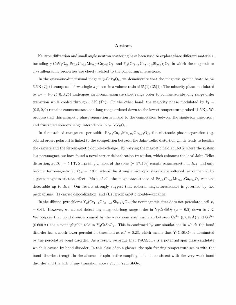
Abstract
Neutron diffraction and small angle neutron scattering have been used to explore three different materials,
including γ-CoV2O6, Pr0.5Ca0.5Mn0.97Ga0.03O3, and Y2(Cr1−xGax−0.5Sb0.5)2O7, in which the magnetic or
crystallographic properties are closely related to the comepting interactions.
In the quasi-one-dimensional magnet γ-CoV2O6, we demonstrate that the magnetic ground state below
6.6 K (TN) is composed of two single-k phases in a volume ratio of 65(1) : 35(1). The minority phase modulated
by k2 = (-0.25, 0, 0.25) undergoes an incommensurate short range order to commensurate long range order
transition while cooled through 5.6 K (T ∗). On the other hand, the majority phase modulated by k1 =
(0.5, 0, 0) remains commensurate and long range ordered down to the lowest temperature probed (1.5 K). We
propose that this magnetic phase separation is linked to the competition between the single-ion anisotropy
and frustrated spin exchange interactions in γ-CoV2O6.
In the strained manganese perovskite Pr0.5Ca0.5Mn0.97Ga0.03O3, the electronic phase separation (e.g.
orbital order, polaron) is linked to the competition between the Jahn-Teller distortion which tends to localize
the carriers and the ferromagnetic double-exchange. By varying the magnetic field at 150 K where the system
is a paramagnet, we have found a novel carrier delocalization transition, which enhances the local Jahn-Teller
distortion, at Bc1 = 5.1 T. Surprisingly, most of the spins (∼ 97.5 %) remain paramagnetic at Bc1, and only
become ferromagnetic at Bc2 = 7.9 T, where the strong anisotropic strains are softened, accompanied by
a giant magnetostriction effect. Most of all, the magnetoresistance of Pr0.5Ca0.5Mn0.97Ga0.03O3 remains
detectable up to Bc2. Our results strongly suggest that colossal magnetoresistance is governed by two
mechanisms: (I) carrier delocalization, and (II) ferromagnetic double-exchange.
In the diluted pyrochlores Y2(Cr1−xGax−0.5Sb0.5)2O7, the nonmagnetic sites does not percolate until xc
= 0.61. However, we cannot detect any magnetic long range order in Y2CrSbO7 (x = 0.5) down to 2 K.
We propose that bond disorder caused by the weak ionic size mismatch between Cr3+ (0.615 A) and Ga5+
(0.600 A) has a nonnegligible role in Y2CrSbO7. This is confirmed by our simulations in which the bond
disorder has a much lower percolation threshold at xc’ = 0.23, which means that Y2CrSbO7 is dominated
by the percolative bond disorder. As a result, we argue that Y2CrSbO7 is a potential spin glass candidate
which is caused by bond disorder. In this class of spin glasses, the spin freezing temperature scales with the
bond disorder strength in the absence of spin-lattice coupling. This is consistent with the very weak bond
disorder and the lack of any transition above 2 K in Y2CrSbO7.

for my great grandmother Lindi Sheng
ACKNOWLEDGEMENTS
First and foremost, I would like to say uncountable ‘Thanks’ to my parents, Dakai Shen and Jingxiao Tao,
for their invaluable support since my birth. By ‘measuring’ their granddaughter, Jessica Shen, I can feel the
hard work her grandparents have done to her father!
As a PhD student, I have had a fantastic time in the Birmingham condensed matter group. I acknowledge
my doctoral supervisor Elizabeth Blackburn for offering me a position and her invaluable support in this
period. I am especially grateful that I was allowed to focus on my personal research interests in my PhD
program. I also would like to thank Ted Forgan. It seems to us that he knows everything. And as a man in
his 70s, he definitely runs faster than the average. I thank both Elizabeth and Ted for getting me involved in
the 17-Tesla magnet project, in which I have learnt the very great importance of being patient and careful.
This PhD program is based on a wide range of collaboration. I would like to thank the scientists at the
large facilities I have used. These include Sebastian MuhlBauer, Andre Heinemann, Astrid Schneidewind,
Petr Cermak, Jurg Schefer, Oksana Zaharko, Jonas Okkels Birk, Urs Gasser, Jorge Gavilano, Emmanuel
Canevet, Thomas Prokscha, Thomas Hansen, Charles Dewhurst, Eric Ressouche, Marek Bartkowiak, Markus
Zolliker, Pascal Manuel, Dmitry Khalyavin, Peter Baker, Gavin Stenning, etc. I also thank Zhangzhen He
and Mitsuru Itoh for kindly providing me their crystals. I would particularly like to thank Mark Laver, who
not only taught me how to write a scientific paper, but also offered me many inspiring career suggestions.
I would like to thank other members of the Birmingham condensed matter group I have worked with:
Alex Holmes, Josh Lim, Alistair Cameron, Bindu Malini Gunupudi, Louis Lemberger, Randeep Riyat, Erik
Jellyman, Michael Parkes, and Jonathan Perrins. Alex Holmes always told me ‘Think twice before you do
it!’. Josh Lim was a very good tutor during my first year. Alistair Cameron gave me the first lesson of how
to lead an experiment. Bindu Malini Gunupudi was a good listener. Louis Lemberger proposed a curry tour
everytime when he went back from Institut Laue-Langevin (ILL). Randeep Riyat was always happy to offer
me a ride when there was a heavy rain after work. Erik Jellyman offered me some pills to kill my fever during
a very stressful beamtime. Michael Parkes was always able to provide the liquid helium in time. Jonathan

Perrins made some very useful sample holders for me.
Last but not the least, I thank my wife, Yunqing Zhang, for her effort of supporting and expanding the
family in Birmingham. We came to Birmingham on 13th September, 2012 as a ‘duo’. Four years later, we
are almost ready to be a ‘quartet’ !
22 : 39, 13th September, 2016.
CONTENTS
1 Introduction 1
1.1 Fundamental concepts . . . . . . . . . . . . . . . . . . . . . . . . . . . . . . . . . . . . . . . . 1
1.1.1 Orbital angular momentum . . . . . . . . . . . . . . . . . . . . . . . . . . . . . . . . . 1
1.1.2 Spin angular momentum . . . . . . . . . . . . . . . . . . . . . . . . . . . . . . . . . . . 4
1.1.3 Total angular momentum . . . . . . . . . . . . . . . . . . . . . . . . . . . . . . . . . . 4
1.1.4 Paramagnetism . . . . . . . . . . . . . . . . . . . . . . . . . . . . . . . . . . . . . . . . 5
1.1.5 Crystal fields . . . . . . . . . . . . . . . . . . . . . . . . . . . . . . . . . . . . . . . . . 7
1.1.6 Jahn-Teller distortion . . . . . . . . . . . . . . . . . . . . . . . . . . . . . . . . . . . . 8
1.2 Interactions . . . . . . . . . . . . . . . . . . . . . . . . . . . . . . . . . . . . . . . . . . . . . . 9
1.2.1 Coulomb interactions . . . . . . . . . . . . . . . . . . . . . . . . . . . . . . . . . . . . 9
1.2.2 Exchange interactions . . . . . . . . . . . . . . . . . . . . . . . . . . . . . . . . . . . . 10
1.2.3 Dzyaloshinsky-Moriya interaction . . . . . . . . . . . . . . . . . . . . . . . . . . . . . . 13
1.2.4 Magnetic dipolar interaction . . . . . . . . . . . . . . . . . . . . . . . . . . . . . . . . 13
1.2.5 Spin-orbit coupling . . . . . . . . . . . . . . . . . . . . . . . . . . . . . . . . . . . . . . 13
1.2.6 Electron-phonon coupling . . . . . . . . . . . . . . . . . . . . . . . . . . . . . . . . . . 14
1.2.7 Ruderman-Kittel-Kasuya-Yosida interaction . . . . . . . . . . . . . . . . . . . . . . . . 15
1.3 Frustrated magnetism . . . . . . . . . . . . . . . . . . . . . . . . . . . . . . . . . . . . . . . . 15
1.3.1 Geometric frustration . . . . . . . . . . . . . . . . . . . . . . . . . . . . . . . . . . . . 15
1.3.2 Spin glass in Y2Mo2O7 . . . . . . . . . . . . . . . . . . . . . . . . . . . . . . . . . . . 16
1.3.3 Long range order in Y2Mn2O7 . . . . . . . . . . . . . . . . . . . . . . . . . . . . . . . 20
1.4 Phase separation . . . . . . . . . . . . . . . . . . . . . . . . . . . . . . . . . . . . . . . . . . . 21
1.4.1 Dynamic phase separation in Ca3Co2O6 . . . . . . . . . . . . . . . . . . . . . . . . . . 22
1.4.2 Mixed-valence perovskite manganites . . . . . . . . . . . . . . . . . . . . . . . . . . . . 24

2 Experimental Techniques 31
2.1 Sample synthesis . . . . . . . . . . . . . . . . . . . . . . . . . . . . . . . . . . . . . . . . . . . 31
2.2 Scattering techniques . . . . . . . . . . . . . . . . . . . . . . . . . . . . . . . . . . . . . . . . . 31
2.2.1 Basic scattering theory . . . . . . . . . . . . . . . . . . . . . . . . . . . . . . . . . . . . 32
2.2.2 X-ray powder diffraction . . . . . . . . . . . . . . . . . . . . . . . . . . . . . . . . . . . 34
2.2.3 Neutron powder diffraction . . . . . . . . . . . . . . . . . . . . . . . . . . . . . . . . . 36
2.2.4 Small angle neutron scattering . . . . . . . . . . . . . . . . . . . . . . . . . . . . . . . 40
2.3 Magnetometry . . . . . . . . . . . . . . . . . . . . . . . . . . . . . . . . . . . . . . . . . . . . 42
2.3.1 Magnetic Property Measurement System (MPMS) . . . . . . . . . . . . . . . . . . . . 42
2.3.2 Vibrating Sample Magnetometer (VSM) . . . . . . . . . . . . . . . . . . . . . . . . . . 43
2.4 Physical Property Measurement System (PPMS) . . . . . . . . . . . . . . . . . . . . . . . . . 44
3 A quasi-one-dimensional magnet, γ-CoV2O6 46
3.1 Background . . . . . . . . . . . . . . . . . . . . . . . . . . . . . . . . . . . . . . . . . . . . . . 46
3.1.1 Magnetic structure of α-CoV2O6 . . . . . . . . . . . . . . . . . . . . . . . . . . . . . . 46
3.1.2 Previous investigations on γ-CoV2O6: a 2-k Ising magnet? . . . . . . . . . . . . . . . 51
3.2 Results . . . . . . . . . . . . . . . . . . . . . . . . . . . . . . . . . . . . . . . . . . . . . . . . . 56
3.2.1 Research motivations . . . . . . . . . . . . . . . . . . . . . . . . . . . . . . . . . . . . . 56
3.2.2 Data collection and analysis . . . . . . . . . . . . . . . . . . . . . . . . . . . . . . . . . 57
3.2.3 Magnetic phase separation in γ-CoV2O6 . . . . . . . . . . . . . . . . . . . . . . . . . . 61
3.3 Conclusions and future work . . . . . . . . . . . . . . . . . . . . . . . . . . . . . . . . . . . . 71
4 Mixed-valence manganese perovskite, Pr0.5Ca0.5Mn0.97Ga0.03O3 72
4.1 Background . . . . . . . . . . . . . . . . . . . . . . . . . . . . . . . . . . . . . . . . . . . . . . 72
4.1.1 Multiple scale phase separation and colossal magnetoresistance . . . . . . . . . . . . . 72
4.1.2 Electronic phase separation and magnetostriction . . . . . . . . . . . . . . . . . . . . . 75
4.1.3 Electronic phase separation and Jahn-Teller distortion . . . . . . . . . . . . . . . . . . 77
4.1.4 Pr0.5Ca0.5Mn1−xMxO3, M = Ga, Al, Co, Ti, etc . . . . . . . . . . . . . . . . . . . . . . 79
4.2 Results . . . . . . . . . . . . . . . . . . . . . . . . . . . . . . . . . . . . . . . . . . . . . . . . . 83
4.2.1 Research motivations . . . . . . . . . . . . . . . . . . . . . . . . . . . . . . . . . . . . . 83
4.2.2 Data analysis . . . . . . . . . . . . . . . . . . . . . . . . . . . . . . . . . . . . . . . . . 84
4.2.3 Zero field magnetism at T = 150 K . . . . . . . . . . . . . . . . . . . . . . . . . . . . . 95
4.2.4 Magnetoresistance and magnetic field dependence of magnetization at T = 150 K . . . 97
4.2.5 Collapse of electronic phase separation induced by magnetic field at T = 150 K . . . . 100
4.2.6 Discussion . . . . . . . . . . . . . . . . . . . . . . . . . . . . . . . . . . . . . . . . . . . 103
4.3 Conclusions and future work . . . . . . . . . . . . . . . . . . . . . . . . . . . . . . . . . . . . 107
5 Diluted pyrochlore, Y2(Cr1−xGax−0.5Sb0.5)2O7 109
5.1 Background . . . . . . . . . . . . . . . . . . . . . . . . . . . . . . . . . . . . . . . . . . . . . . 109
5.1.1 Magnetic 3d transition-metal pyrochlores . . . . . . . . . . . . . . . . . . . . . . . . . 109
5.1.2 Structural disorder and magnetism . . . . . . . . . . . . . . . . . . . . . . . . . . . . . 111
5.1.3 RE2(Cr0.5Sb0.5)2O7, RE = Ho, Y, Dy, Tb, Er, etc . . . . . . . . . . . . . . . . . . . . . . 114
5.2 Results . . . . . . . . . . . . . . . . . . . . . . . . . . . . . . . . . . . . . . . . . . . . . . . . . 115
5.2.1 Research motivations . . . . . . . . . . . . . . . . . . . . . . . . . . . . . . . . . . . . . 115
5.2.2 Data analysis . . . . . . . . . . . . . . . . . . . . . . . . . . . . . . . . . . . . . . . . . 116
5.2.3 Absence of magnetic order in Y2(Cr0.5Sb0.5)2O7: a spin glass candidate . . . . . . . . 117
5.3 Conclusions and future work . . . . . . . . . . . . . . . . . . . . . . . . . . . . . . . . . . . . 127
6 Summary 128
6.1 γ-CoV2O6 . . . . . . . . . . . . . . . . . . . . . . . . . . . . . . . . . . . . . . . . . . . . . . . 128
6.2 Pr0.5Ca0.5Mn0.97Ga0.03O3 . . . . . . . . . . . . . . . . . . . . . . . . . . . . . . . . . . . . . . 128
6.3 Y2(Cr1−xGax−0.5Sb0.5)2O7, 0.56 x 6 0.9 . . . . . . . . . . . . . . . . . . . . . . . . . . . . . . 129
Appendix A Rietveld refinement I
List of References III
LIST OF FIGURES
1.1 Angular distribution of s, p, d orbitals, from Ref. [3]. . . . . . . . . . . . . . . . . . . . . . . . 2
1.2 (a) MO6-octahedron. M = TM ion (black solid). Oxygens are red solids. The orthogonal axes
are also labelled. (b) Crystal field splitting of the d orbitals. . . . . . . . . . . . . . . . . . . . 7
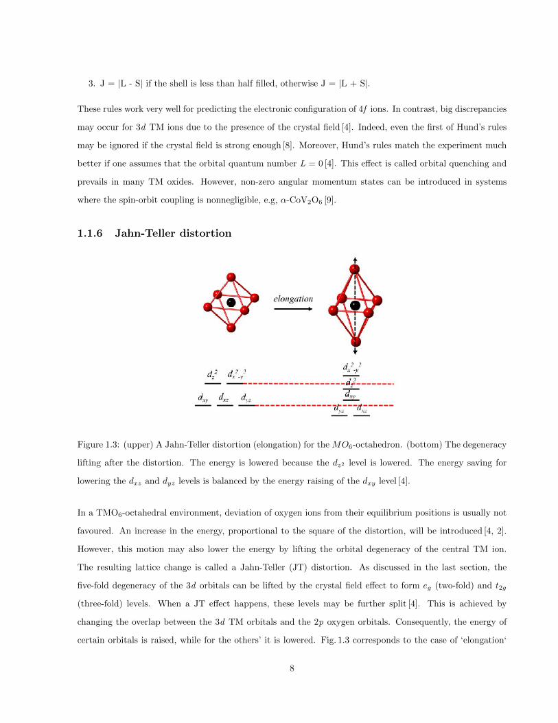
1.3 (upper) A Jahn-Teller distortion (elongation) for the MO6-octahedron. (bottom) The degen-
eracy lifting after the distortion. The energy is lowered because the dz2 level is lowered. The
energy saving for lowering the dxz and dyz levels is balanced by the energy raising of the dxy
level [4]. . . . . . . . . . . . . . . . . . . . . . . . . . . . . . . . . . . . . . . . . . . . . . . . . 8
1.4 Superexchange process. The electron hopping is marked by dashed arrows. Antiferromagnetic
spin alignment is achieved in this one-orbital model. . . . . . . . . . . . . . . . . . . . . . . . 11
1.5 Double exchange mechanism in mixed-valence oxides. . . . . . . . . . . . . . . . . . . . . . . . 12
1.6 Two eg-active JT modes. . . . . . . . . . . . . . . . . . . . . . . . . . . . . . . . . . . . . . . 14
1.7 (a) Antiferromagnetically coupled spins on a triangular (upper) or tetrahedral (bottom) lattice
unit. Corner-sharing tetrahedral sublattices in a pyrochlore structure (shaded) formed by (b)
A (green solids), and (c) B (blue solids) ions [19]. Oxygen ions are omitted. . . . . . . . . . . 16
1.8 SG behaviour in a Cu1−xMnx alloy [20]. Temperature dependences of (a) ac susceptibility, (b)
heat capacity, and (c) ZFC (branch b and d) and FC (branch a and c) dc susceptibility curves.
(d) Spin relaxation at various temperatures, where ~S(~q, t) ∝< ~Si(t)·~Sj(0) >T exp[i~q·(~ri − ~rj)]
and q = 0.093 A−1. . . . . . . . . . . . . . . . . . . . . . . . . . . . . . . . . . . . . . . . . . . 17
1.9 (Left) Inverse susceptibililty versus temperature (solids) curve of Y2Mo2O7. The black line is a
linear fit to its high temperature part [21]. (Top right) ZFC and FC curves when B = 0.01 T [23].
(Bottom right) Nonlinear susceptibility χnl analyzed according to the critical scaling model in
Ref. [23] . . . . . . . . . . . . . . . . . . . . . . . . . . . . . . . . . . . . . . . . . . . . . . . . 18
1.10 (Left) Low energy inelastic neutron spectrum of Y2Mo2O7 at different temperatures [22].
(Right) Elastic magnetic structure factor S(Q) versus scattering vector (Q) plot at 1.4 K [22]. 19

1.11 Heat capacity data measured by Reimers et al [33] (a) and Shimakwa et al [34] (b). (c) ZFC
and FC magnetization versus temperature curves at B = 0.15 mT (circle), 0.56 mT(square) and
10 mT (triangle) [33]. (d) Magnetization versus magnetic field curves at various temperaures.
From top to bottom: 1.8 K, 5 K, 7.5 K, 10 K, 15 K, 20 K, 25 K, 30 K, 35 K, 40 K, 45 K, 50 K [33].
(e) Real and imaginary parts of the ac susceptibility. The inset shows the frequency dependence
at low temperatures [33]. . . . . . . . . . . . . . . . . . . . . . . . . . . . . . . . . . . . . . . . 20
1.12 Small angle neutron scattering measurements on Y2Mn2O7 [35]. (Left) Neutron intensity ver-
sus scattering vector Q at different temperatures (solids). The solid and dotted lines are the
numerical fits using eq. 1.50 with and without the instrumental resolution function. (Right)
Temperature dependences of the two types of magnetic correlation length, ξ1 and ξ2. . . . . . 21
1.13 (a) Crystallographic structure of Ca3Co2O6 [36]. (b) The triangular Co sublattice in the ab-
plane [36]. . . . . . . . . . . . . . . . . . . . . . . . . . . . . . . . . . . . . . . . . . . . . . . 22
1.14 (a) -(b) Dynamic phase separation in Ca3Co2O6 measured by neutron powder diffraction. An
new peak belong to the CAFM phase gradually develops in 6 h of counting time at 10 K [40]. (c)
Small angle neutron scattering patterns at different temperatures. The instrumental resolution
limited peaks along the qc are the first reflections of the SDW phase [39]. The broad steaks
along qab are linked to the ferrimagnetic microphase [42]. . . . . . . . . . . . . . . . . . . . . . 23
1.15 (a) Basic structure of a cubic perovskite with chemical fomula ABO3. (b) Resistance at 300 K
(ρ(300K)) as a function of rA (inset) Curie temperature obtained from ρ versus temperature
curve as a function of ρ(300K) [44]. (c) The ‘universal’ phase diagram defined by the tolerence
factor [44]. . . . . . . . . . . . . . . . . . . . . . . . . . . . . . . . . . . . . . . . . . . . . . . . 24
1.16 (a) Phase diagram of La1−xCaxMnO3 [2], with CAF = canted antiferromagnetism, CO = charge
order, FI = ferromagnetic insulator, FM = ferromagnetic metal and AF = antiferromagnetism.
(b) Magnetization, resistance and magnetoresistance as a function of temperature when x = 0.25 [2]. 25
1.17 (a) Phase diagram of Pr1−xCaxMnO3, with FMI = ferromagnetic insulator, CO = charge order,
AFMI = antiferromagnetic insulator and CG = cluster glass [49]. (b) Resistivity as a function
of magnetic field at various temperatures when x = 0.35 [51]. . . . . . . . . . . . . . . . . . . . 26
1.18 d3x2−r2/d3y2−r2 orbital order under Pbcm space group (a ' b'√
2c) setup [52]. The orbital
orientations of the Mn3+ ions are marked by the lobes. The black and red arrows show the
spin arrangement in the z = 0 plane. The spins in the z = 1/2 plane are reversed (unchanged)
for the CE (pseudo-CE) type antiferromagnetic order [50]. . . . . . . . . . . . . . . . . . . . . 27

1.19 (a)-(b) Resistivity versus temperature curves under different electron-phonon coupling strengths
λ with fixed n. Details of the density parameter n can be found in Ref. [47]. (c)-(d) Resis-
tivity versus temperature curves at various magnetic fields with fixed n [47]. (e) Temperature
dependence of the standard deviation of Mn-O bond lengths in La1−xCaxMnO3 measured by
Booth et al. [53]. Clear softening of the distortion is observed below TC. . . . . . . . . . . . . 28
1.20 (Top-left) Schematic view of the Ln0.5Ba0.5MnO3 lattice in the ac-plane, where the a-axis
is horizontal [59]. (Bottom-left) Magnetization and resisitivity of the two end compounds as
a function of temperature [59]. (Top-right) Dark field images of La5/8−yPryCa3/8MnO3 [60].
The charge disordered ferromagnetic area is dark. (a) y = 0.375 and T = 20 K (ferromagnetic).
(b) y = 0.4 and T = 17 K (ferromagnetic). (c) y = 0.4 and T = 120 K (Paramagnetic). (Bottom-
right) Schematic show of the percolation process as a function of magnetic field [60]. . . . . . 29
2.1 Geometry for a scattering process. . . . . . . . . . . . . . . . . . . . . . . . . . . . . . . . . . 32
2.2 (a) Distribution of X-ray emission intensity as a function of wavelength. The broad background
with a lower limit is Bremsstrahlung. The sharp peaks are from the relaxation process. (b)
Typical relaxation processes (purple solid line) after the electron in the K -shell (E1) is emitted
(red dotted line). . . . . . . . . . . . . . . . . . . . . . . . . . . . . . . . . . . . . . . . . . . . 34
2.3 Schematic demonstrations of (a) fission [67], and (b) spallation processes [68]. . . . . . . . . . 36
2.4 Experimental setup of the D20 2-axis diffractometer at ILL, France [70]. . . . . . . . . . . . . 38
2.5 Coherent nuclear scattering length b as a function of atomic number Z [71]. . . . . . . . . . . 39
2.6 The SANS-1 instrument at FRM-II, Germany [75]. . . . . . . . . . . . . . . . . . . . . . . . . 41
2.7 (a) A SQUID is formed by two parallel Josephson junctions [77]. (b) Working mechanism of
the SQUID. Any weak change in the flux signal will be detected in the output voltage channel
as well [77]. . . . . . . . . . . . . . . . . . . . . . . . . . . . . . . . . . . . . . . . . . . . . . . 42
2.8 Schematic construction of a VSM [79]. . . . . . . . . . . . . . . . . . . . . . . . . . . . . . . . 43
2.9 Schematic representation of a four-point probe array [80]. . . . . . . . . . . . . . . . . . . . . 44
3.1 (Left) Crystallographic structure of αCVO. Edge-sharing CoO6 octahedral chains run along
the b-axis. V and O(3) cites are omitted for clarity. (Right) Projection of the Co-sites in the
ac-plane. The triangular arrangement allows geometric frustration. . . . . . . . . . . . . . . . 46

3.2 (a) Temperature dependence of the magnetic susceptibilities of αCVO. The solid line is a fit
using the Ising chain model described in Ref. [86]. (b) Magnetization versus magnetic field
curves taken at 5 K. . . . . . . . . . . . . . . . . . . . . . . . . . . . . . . . . . . . . . . . . . 48
3.3 (a) The CoO6-octahedron distortion in αCVO and the schematic crystal field levels [9]. (b)
Spin exchange paths between Co ions [85]. Interchain and intrachain couplings are in blue and
red, respectively. . . . . . . . . . . . . . . . . . . . . . . . . . . . . . . . . . . . . . . . . . . . 48
3.4 (a) Simulated magnetization versus magnetic field curve [85]. Inset: the corresponding mag-
netic structures in the ac-plane. (b) Magnetic field dependence of lattice parameters (p
=a, b, c,β and Volume) [91]. . . . . . . . . . . . . . . . . . . . . . . . . . . . . . . . . . . . . . 49
3.5 Left: Co-chains along the b-axis in γCVO. Right: Projection of the Co-sites in the ac-plane. . 51
3.6 (a) Heat capacity data of αCVO and γCVO [101]. (b) and (c) Magnetization curves of γCVO
single-crystal and powder [99]. The (b) magnetic field, and (c) temperature scans were taken
at T = 1.8 K and B = 0.1 T, respectively. . . . . . . . . . . . . . . . . . . . . . . . . . . . . . . 53
3.7 Neutron powder diffraction patterns collected by Kimber et al [98] at (a) λ= 2.8 A, T = 2 K
and (b) λ= 1.79 A, T = 2 K and Lenertz et al [99] at (c) λ= 2.423 A, T = 1.7 K. . . . . . . . . 54
3.8 (a) Local CoO6 enviroments of γCVO and the schematic crystal field level splitting [9]. Mag-
netic phase diagram of (a) αCVO and (b) γCVO [101]. . . . . . . . . . . . . . . . . . . . . . . 55
3.9 Single-crystal diffraction patterns of γCVO collected at λ= 2.31 A, T = 1.5 K. . . . . . . . . . 56
3.10 Powder diffraction patterns obtained at T = 1.5 K. The calculated pattern (black solid lines)
correspond to the first step described in the context. The vertical bars, from top to bottom,
label the reflections of nuclear, k1, k2 and Aluminium (sample holder), respectively. The
Rietveld factors (Appendix A) are also displayed. . . . . . . . . . . . . . . . . . . . . . . . . . 59
3.11 Evolution of the Rietveld factors of the neutron diffraction pattern at λ= 4.5 A in the refine-
ment process. . . . . . . . . . . . . . . . . . . . . . . . . . . . . . . . . . . . . . . . . . . . . . 60
3.12 (a) Crystal structure of triclinic γCVO. Oxygen anions (omitted for clarity) occupy the corner
of the shaded polyhedra. (b) Possible interchain spin exchange paths displayed in two unit
cells for Co(1) and Co(2), respectively. . . . . . . . . . . . . . . . . . . . . . . . . . . . . . . . 62
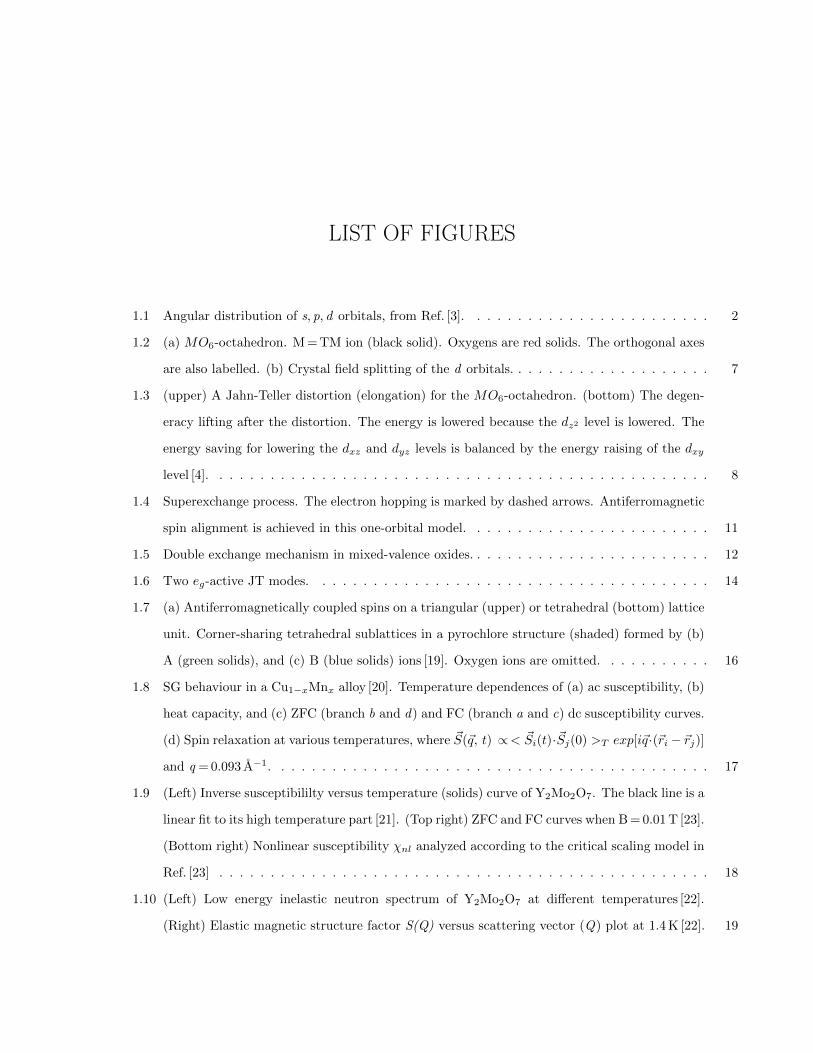
3.13 Neutron powder diffraction pattern measured at λ= 4.5 A, T = 1.5 K. The red solid dots are
experimental observations. The black and blue lines are the calculated pattern and the dif-
ference using the 2 -phase model. Black, pink and green vertical bars mark the nuclear, k1-
and k2- modulated Bragg positions, respectively. Right inset: Sketch of the ac-plane magnetic
structure modulated by k2 in a 5x5 unit cell. Left inset: A weak reflection indexed as (0.5, 1, 0)
around 0.931 A. . . . . . . . . . . . . . . . . . . . . . . . . . . . . . . . . . . . . . . . . . . . . 63
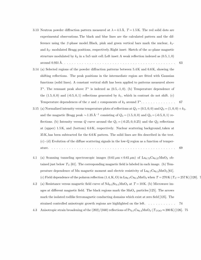
3.14 (a) Selected regions of the powder diffraction patterns between 5.4 K and 6.6 K, showing the
shifting reflections. The peak positions in the intermediate region are fitted with Gaussian
functions (solid lines). A constant vertical shift has been applied to patterns measured above
T ∗. The remnant peak above T ∗ is indexed as (0.5, -1, 0). (b) Temperature dependence of
the (1.5, 0, 0) and (-0.5, 0, 1) reflections generated by k1, which in contrast do not shift. (c)
Temperature dependences of the x and z components of k2 around T ∗. . . . . . . . . . . . . . 67
3.15 (a) Normalized intensity versus temperature plots of reflections atQ2 = (0.5, 0, 0) andQ3 = (1, 0, 0) + k2,
and the magnetic Bragg peak ∼ 1.35 A−1 consisting of Q4 = (1.5, 0, 0) and Q5 = (-0.5, 0, 1) re-
flections. (b) Intensity versus Q curve around the Q1 = (-0.25, 0, 0.25) and the Q2 reflections
at (upper) 1.5 K, and (bottom) 6.6 K, respectively. Nuclear scattering background, taken at
35 K, has been subtracted for the 6.6 K pattern. The solid lines are fits described in the text.
(c) - (d) Evolution of the diffuse scattering signals in the low-Q region as a function of temper-
ature. . . . . . . . . . . . . . . . . . . . . . . . . . . . . . . . . . . . . . . . . . . . . . . . . . 69
4.1 (a) Scanning tunneling spectroscopic images (0.61µm× 0.61µm) of La0.73Ca0.27MnO3 ob-
tained just below TC [61]. The corresponding magnetic field is labeled in each image. (b) Tem-
perature dependence of Mn magnetic moment and electric resistivity of La0.7Ca0.3MnO3 [61].
(c) Field dependence of the polaron reflection (1.4, K, O) in La0.7Ca0.3MnO3 when T = 270 K (TC = 257 K) [120]. 73
4.2 (a) Resistance versus magnetic field curve of Nd0.5Sr0.5MnO3 at T = 10 K. (b) Microwave im-
ages at different magnetic field. The black regions mark the MnOx particles [125]. The arrows
mark the isolated rodlike ferromagnetic conducting domains which exist at zero field [125]. The
strained controlled anisotropic growth regions are highlighted on the left. . . . . . . . . . . . 74
4.3 Anisotropic strain broadening of the (202)/(040) reflections of Pr0.7Ca0.3MnO3 (TCOO≈ 200 K) [126]. 75
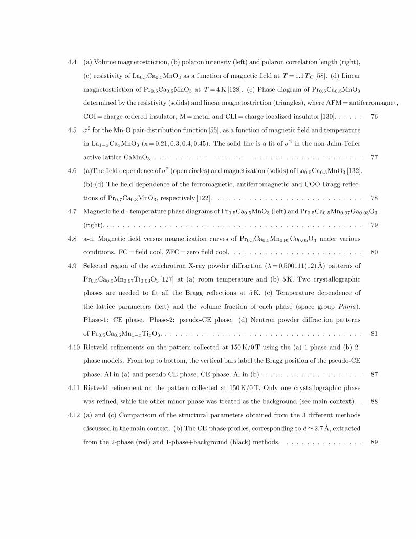
4.4 (a) Volume magnetostriction, (b) polaron intensity (left) and polaron correlation length (right),
(c) resistivity of La0.5Ca0.5MnO3 as a function of magnetic field at T = 1.1TC [58]. (d) Linear
magnetostriction of Pr0.5Ca0.5MnO3 at T = 4 K [128]. (e) Phase diagram of Pr0.5Ca0.5MnO3
determined by the resistivity (solids) and linear magnetostriction (triangles), where AFM = antiferromagnet,
COI = charge ordered insulator, M = metal and CLI = charge localized insulator [130]. . . . . . 76
4.5 σ2 for the Mn-O pair-distribution function [55], as a function of magnetic field and temperature
in La1−xCaxMnO3 (x = 0.21, 0.3, 0.4, 0.45). The solid line is a fit of σ2 in the non-Jahn-Teller
active lattice CaMnO3. . . . . . . . . . . . . . . . . . . . . . . . . . . . . . . . . . . . . . . . . 77
4.6 (a)The field dependence of σ2 (open circles) and magnetization (solids) of La0.5Ca0.5MnO3 [132].
(b)-(d) The field dependence of the ferromagnetic, antiferromagnetic and COO Bragg reflec-
tions of Pr0.7Ca0.3MnO3, respectively [122]. . . . . . . . . . . . . . . . . . . . . . . . . . . . . 78
4.7 Magnetic field - temperature phase diagrams of Pr0.5Ca0.5MnO3 (left) and Pr0.5Ca0.5Mn0.97Ga0.03O3
(right). . . . . . . . . . . . . . . . . . . . . . . . . . . . . . . . . . . . . . . . . . . . . . . . . . 79
4.8 a-d, Magnetic field versus magnetization curves of Pr0.5Ca0.5Mn0.95Co0.05O3 under various
conditions. FC = field cool, ZFC = zero field cool. . . . . . . . . . . . . . . . . . . . . . . . . . 80
4.9 Selected region of the synchrotron X-ray powder diffraction (λ= 0.500111(12) A) patterns of
Pr0.5Ca0.5Mn0.97Ti0.03O3 [127] at (a) room temperature and (b) 5 K. Two crystallographic
phases are needed to fit all the Bragg reflections at 5 K. (c) Temperature dependence of
the lattice parameters (left) and the volume fraction of each phase (space group Pnma).
Phase-1: CE phase. Phase-2: pseudo-CE phase. (d) Neutron powder diffraction patterns
of Pr0.5Ca0.5Mn1−xTixO3. . . . . . . . . . . . . . . . . . . . . . . . . . . . . . . . . . . . . . . 81
4.10 Rietveld refinements on the pattern collected at 150 K/0 T using the (a) 1-phase and (b) 2-
phase models. From top to bottom, the vertical bars label the Bragg position of the pseudo-CE
phase, Al in (a) and pseudo-CE phase, CE phase, Al in (b). . . . . . . . . . . . . . . . . . . . 87
4.11 Rietveld refinement on the pattern collected at 150 K/0 T. Only one crystallographic phase
was refined, while the other minor phase was treated as the background (see main context). . 88
4.12 (a) and (c) Comparisom of the structural parameters obtained from the 3 different methods
discussed in the main context. (b) The CE-phase profiles, corresponding to d ' 2.7 A, extracted
from the 2-phase (red) and 1-phase+background (black) methods. . . . . . . . . . . . . . . . 89

4.13 Main panel, Rietveld refinement of the pattern collected at 150 K/8 T. Inset: A comparison
between the 150 K/8 T and 150 K/0 T patterns. The absence of (0, 1, 1) peak clearly indicates
the preferential orientation of the spins with respect to the crystallographic structure. . . . . 90
4.14 The scattering geometry in a SANS experiment. The magnetic field is along the z -axis. The
scattering vector is denoted as q. . . . . . . . . . . . . . . . . . . . . . . . . . . . . . . . . . . 91
4.15 T = 150 K, B = 2 T. (a) I (q)-q curves under different instrumental configurations. (b) The
merged curve. The shaded areas mark the overlapping regions. . . . . . . . . . . . . . . . . . 93
4.16 (a) I (q) versus q curve at 150 K/2 T under the horizontal field setup and the simulated con-
tributions using eq. 4.9. (b) I (q) versus q curve at 150 K/10 T under the vertical field setup
and the simulated contributions using eq. 4.7. . . . . . . . . . . . . . . . . . . . . . . . . . . . 94
4.17 Main panel: ZFC and FC curves of PCMGO recorded on warming under B = 0.05 T. The
bump marked by the double arrow is caused by a minor impurity phase identified as Mn3O4
(see main text). Inset: Inverse ZFC susceptibility versus temperature curve (open circles).
Its linear part above ∼ 350 K has been fitted by the CW law (dotted line). The hatched area
marks the onset of ferromagnetism. . . . . . . . . . . . . . . . . . . . . . . . . . . . . . . . . . 95
4.18 Zero field TOF-NPD pattern of PCMGO collected at 10 K (red) and 150 K (blue), respectively.
The antiferromagnetic Bragg reflections at large d-spacings have been indexed. The black
arrows mark the ferromagnetic Bragg positions. The additional peak around 4.93 A is the
magnetic Bragg reflection of Mn3O4 (see main text). . . . . . . . . . . . . . . . . . . . . . . . 96
4.19 Resistance (R) versus magnetic field curve and the derivatives (dR
dB) of PCMGO at 150 K. The
critical fields B1 and B2 are labeled by vertical lines (see main context). . . . . . . . . . . . . 97
4.20 Main panel: Magnetization versus magnetic field curve (red line) of PCMGO at 150 K. The
black arrows mark the field sweeping direction. The blue line is a linear fit to the low field
part where the system is paramagnetic. The critical fields B1 and B2 are labeled by vertical
lines (see main context). Inset: Enlarged version of the shaded area in the main panel. . . . . 98
4.21 The magnetic field dependences of SANS patterns of PCMGO under the same scale (100 – 900
neutron counts per standard monitor). Each patterm covers a q-range from -0.2 A−1 to 0.2 A−1
in both directions. The narrow vertical slit on the left of each pattern is coming from a dead
detector tube. . . . . . . . . . . . . . . . . . . . . . . . . . . . . . . . . . . . . . . . . . . . . . 100
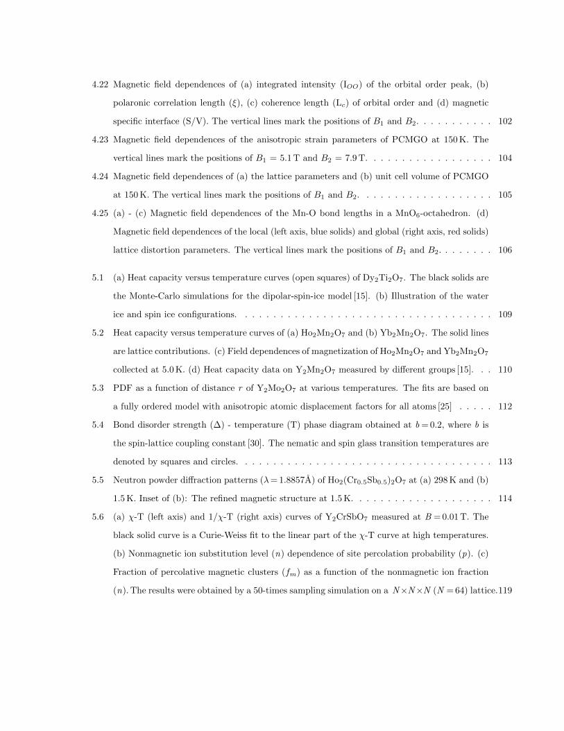
4.22 Magnetic field dependences of (a) integrated intensity (IOO) of the orbital order peak, (b)
polaronic correlation length (ξ), (c) coherence length (Lc) of orbital order and (d) magnetic
specific interface (S/V). The vertical lines mark the positions of B1 and B2. . . . . . . . . . . 102
4.23 Magnetic field dependences of the anisotropic strain parameters of PCMGO at 150 K. The
vertical lines mark the positions of B1 = 5.1 T and B2 = 7.9 T. . . . . . . . . . . . . . . . . . 104
4.24 Magnetic field dependences of (a) the lattice parameters and (b) unit cell volume of PCMGO
at 150 K. The vertical lines mark the positions of B1 and B2. . . . . . . . . . . . . . . . . . . 105
4.25 (a) - (c) Magnetic field dependences of the Mn-O bond lengths in a MnO6-octahedron. (d)
Magnetic field dependences of the local (left axis, blue solids) and global (right axis, red solids)
lattice distortion parameters. The vertical lines mark the positions of B1 and B2. . . . . . . . 106
5.1 (a) Heat capacity versus temperature curves (open squares) of Dy2Ti2O7. The black solids are
the Monte-Carlo simulations for the dipolar-spin-ice model [15]. (b) Illustration of the water
ice and spin ice configurations. . . . . . . . . . . . . . . . . . . . . . . . . . . . . . . . . . . . 109
5.2 Heat capacity versus temperature curves of (a) Ho2Mn2O7 and (b) Yb2Mn2O7. The solid lines
are lattice contributions. (c) Field dependences of magnetization of Ho2Mn2O7 and Yb2Mn2O7
collected at 5.0 K. (d) Heat capacity data on Y2Mn2O7 measured by different groups [15]. . . 110
5.3 PDF as a function of distance r of Y2Mo2O7 at various temperatures. The fits are based on
a fully ordered model with anisotropic atomic displacement factors for all atoms [25] . . . . . 112
5.4 Bond disorder strength (∆) - temperature (T) phase diagram obtained at b = 0.2, where b is
the spin-lattice coupling constant [30]. The nematic and spin glass transition temperatures are
denoted by squares and circles. . . . . . . . . . . . . . . . . . . . . . . . . . . . . . . . . . . . 113
5.5 Neutron powder diffraction patterns (λ= 1.8857A) of Ho2(Cr0.5Sb0.5)2O7 at (a) 298 K and (b)
1.5 K. Inset of (b): The refined magnetic structure at 1.5 K. . . . . . . . . . . . . . . . . . . . 114
5.6 (a) χ-T (left axis) and 1/χ-T (right axis) curves of Y2CrSbO7 measured at B = 0.01 T. The
black solid curve is a Curie-Weiss fit to the linear part of the χ-T curve at high temperatures.
(b) Nonmagnetic ion substitution level (n) dependence of site percolation probability (p). (c)
Fraction of percolative magnetic clusters (fm) as a function of the nonmagnetic ion fraction
(n). The results were obtained by a 50-times sampling simulation on a N×N×N (N = 64) lattice.119

5.7 (main panel) HRNPD pattern (red solids) of Y2CrSbO7 at T = 2.0 K, B = 0 T. Calculated
pattern (black line), nuclear Bragg positions (blue vertical line) and difference (purple line)
are also displayed. (inset) Enlarged version of a selected angle region. Additional peaks from
YCrO3 (red arrows) and V (black arrow) can be visualized. . . . . . . . . . . . . . . . . . . . 120
5.8 (a) Magnetization (M) - temperature (T) curve (purple) of Y2CrSbO7 at 5 T. The black solids
is the derivative of the M-T curve. The red arrow marks the position of TC. (b) TC - x plot
(pink). xc is labeled by the red line. . . . . . . . . . . . . . . . . . . . . . . . . . . . . . . . . 122
5.9 (a) Magnetization (M) versus magnetic field (T) curve (red solids) of Y2CrSbO7 at 2 K. The blue
line is a linear fit to the data above 3.5 T. (b) HRNPD pattern and the Rietveld refinement
of Y2CrSbO7 at 2 K/5 T. The blue arrow marks the ferromagnetic reflection at the reciprocal
position (1, 1, 1). . . . . . . . . . . . . . . . . . . . . . . . . . . . . . . . . . . . . . . . . . . . 123
5.10 (a) - (e) Five possible configurations of a single Cr/Sb-tetrahedron. The bonds are displayed
by dual-band cylinders. (f) Possible influence of bond disorder to the local structure in a unit
cell. O2 oxygens (green spheres) will deviate from their average position (translucent green
spheres), producing a random distribution of Cr/Sb-O2-Cr/Sb bond angles in the sample (red
dotted lines). The Cr/Sb-tetrahedral network is linked by black lines. . . . . . . . . . . . . . 125
5.11 (a) Pecolation probability (p) of bond disorder as a function of the nonmagnetic ion fraction
(n). (b) fm - n curve after taking bond disorder into account. The results were obtained by a
100-times sampling simulation on 64×64×64 (black) and 48×48×48 (blue) lattices, respectively.126
LIST OF TABLES
3.1 Refined lattice parameters, atomic positions and isotropic displacement parameters (Uiso) of
αCVO at 300 K [84]. . . . . . . . . . . . . . . . . . . . . . . . . . . . . . . . . . . . . . . . . . 47
3.2 Room temperature lattice parameters, atomic positions and isotropic displacement parameters
(Biso) of γCVO [82]. . . . . . . . . . . . . . . . . . . . . . . . . . . . . . . . . . . . . . . . . . 52
3.3 Irreducible representations of the magnetic little groupGk of the propagation vector k1 = (0.5, 0, 0)
and k2 = (-0.25, 0, 0.25) for γCVO. . . . . . . . . . . . . . . . . . . . . . . . . . . . . . . . . . 58
3.4 Magnetic and lattice parameters of γCVO at T = 1.5 K. Constraints on the spin orientations
for the k2 modulation have been applied; see main text for details. Co(2) is the central inversion
replica of Co(2). The isotropic displacement parameters (Biso) and V atomic positions were
fixed to the values reported in Ref. [98]. Lattice parameters, O and Co positions were refined
using data at λ = 2.4586 A. Three sets of Rietveld factors, corresponding to the minimal
model (•), inequivalent (†) and equivalent (‡) spin canting on Co(2)- and Co(2)- sites, are listed
for the 2-phase scenario. . . . . . . . . . . . . . . . . . . . . . . . . . . . . . . . . . . . . . . . 65
4.1 Volume fractions, unit cell distortions (D) and strain parameters of Pr0.5Ca0.5Mn0.97Ti0.03O3 [127]. 82
4.2 Refined structural parameters of PCMGO under the Pnma space group. The isotropic dis-
placement parameters have been fixed to the values in Ref. [141]. The pattern at 250 K was
refined using the 1-phase model. . . . . . . . . . . . . . . . . . . . . . . . . . . . . . . . . . . 86
5.1 Structural parameters of Y2CrSbO7 and Y2Cr0.4Ga0.6SbO7. The corresponding HRNPD pat-
terns were refined under space group Fd3m (a = b = c, α= β= γ= 90). The only atomic
position needs to be refined is O2 (x, 0.125, 0.125) [177]. . . . . . . . . . . . . . . . . . . . . . 121
CHAPTER 1
INTRODUCTION
Competing interactions in strongly correlated electron systems often lead to many phases which are close,
or even identical, in free energy at low temperatures. As a result, the physical properties are very sensitive to
external perturbations such as doping, magnetic field, pressure, etc [1, 2]. In the first part of this chapter, we
will briefly recall some key concepts in quantum mechanics. With this knowledge, we will demonstrate several
particle-particle interacting ‘forces’, including the Coulomb interaction, spin exchange interactions, spin-orbit
coupling, and so forth. These terms are of particular importance in understanding the physics discussed in
this thesis. Finally, we will show how the competition of these interactions can lead to exotic particle
condensation using several example materials. Following this chapter, there will be a chapter introducing
the various experimental techniques referred to in this thesis. We will then present work illustrating new
potential effects of these competing interactions. Chapter 3 looks at magnetic phase separation in γ-CoV2O6,
a frustrated quasi-one-dimensional magnet. Chapter 4 is mainly about the decoupling of carrier delocalization
and ferromagnetism in the strained manganese perovskite Pr0.5Ca0.5Mn0.97Ga0.03O3. In the final chapter,
we will illustrate the absence of magnetic long range order in the diluted pyrochlore compound Y2CrSbO7.
1.1 Fundamental concepts
1.1.1 Orbital angular momentum
In classical mechanics, the angular momentum (~L) of a macroscopic object is defined as ~L=~r× ~p, where ~p
is the linear momentum and ~r is the spatial position of this object. However, it is necessary to adjust this
formula in order to correctly describe the ‘orbit’ of a microscopic quantum mechanical particle (e.g. atom,
electron). The vector ~L therefore becomes an operator (L) instead: L= i~r×O. Assuming Li (i = x, y, z)
1

is the projection of the orbital momentum along a particular axis so that L2 = L2x + L2
y + L2z, the following
commutation relations are obtained
[Li, L2] = 0, [Li, Lj ] = iεijk~Lk (i 6= j 6= k), (1.1)
Figure 1.1: Angular distribution of s, p, d orbitals, from Ref. [3].
This means that the two operators, Li and L2, share the same set of eigenfunctions
| l, ml >= Ylml(θ, φ) ∝ Pml
l (cosθ)eimlφ, (1.2)
where l (l = 0, 1, 2, ...),ml (ml = −l, −l + 1, ..., 0, ..., l − 1, l),Pml
l (cosθ) and εijk are angular, magnetic
momentum quantum numbers, Legendre polynomials and Levi-Civita symbol, respectively [4, 5]. As we shall
focus on the 3d (l = 2) transition metal (TM) oxides in this thesis, we plot out the angular dependence
of eigenfunctions belonging to s (l = 0), p (l = 1) and d orbitals in Fig. 1.1. Linear combinations of the
eigenfunctions at a fixed l value are used in this figure. For the p orbitals, we have
Yx =1√2
(Y11 + Y1−1), (1.3)
2
Yy =1
i√
2(Y11 − Y1−1), (1.4)
Yz = Y10. (1.5)
For the d orbitals, we have
Yxy =1
i√
2(Y22 − Y2−2), (1.6)
Yx2−y2 =1√2
(Y22 + Y2−2), (1.7)
Yyz =1
i√
2(−Y21 − Y2−1), (1.8)
Yzx =1√2
(−Y21 + Y2−1), (1.9)
Yz2 = Y20. (1.10)
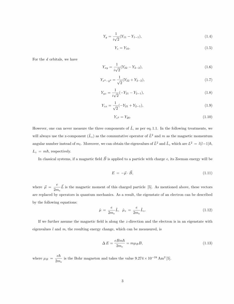
However, one can never measure the three components of L, as per eq. 1.1. In the following treatments, we
will always use the z-component (Lz) as the commutative operator of L2 and m as the magnetic momentum
angular number instead of ml. Moreover, we can obtain the eigenvalues of L2 and Lz which are L2 = l(l−1)~,
Lz = m~, respectively.
In classical systems, if a magnetic field ~B is applied to a particle with charge e, its Zeeman energy will be
E = −~µ · ~B, (1.11)
where ~µ =e
2me
~L is the magnetic moment of this charged particle [5]. As mentioned above, these vectors
are replaced by operators in quantum mechanics. As a result, the eigenstate of an electron can be described
by the following equations:
µ =e
2meL, µz =
e
2meLz. (1.12)
If we further assume the magnetic field is along the z -direction and the electron is in an eigenstate with
eigenvalues l and m, the resulting energy change, which can be meausured, is
∆E =eBm~2me
= mµBB, (1.13)
where µB =e~
2meis the Bohr magneton and takes the value 9.274× 10⁻²⁴ Am2 [5].
3
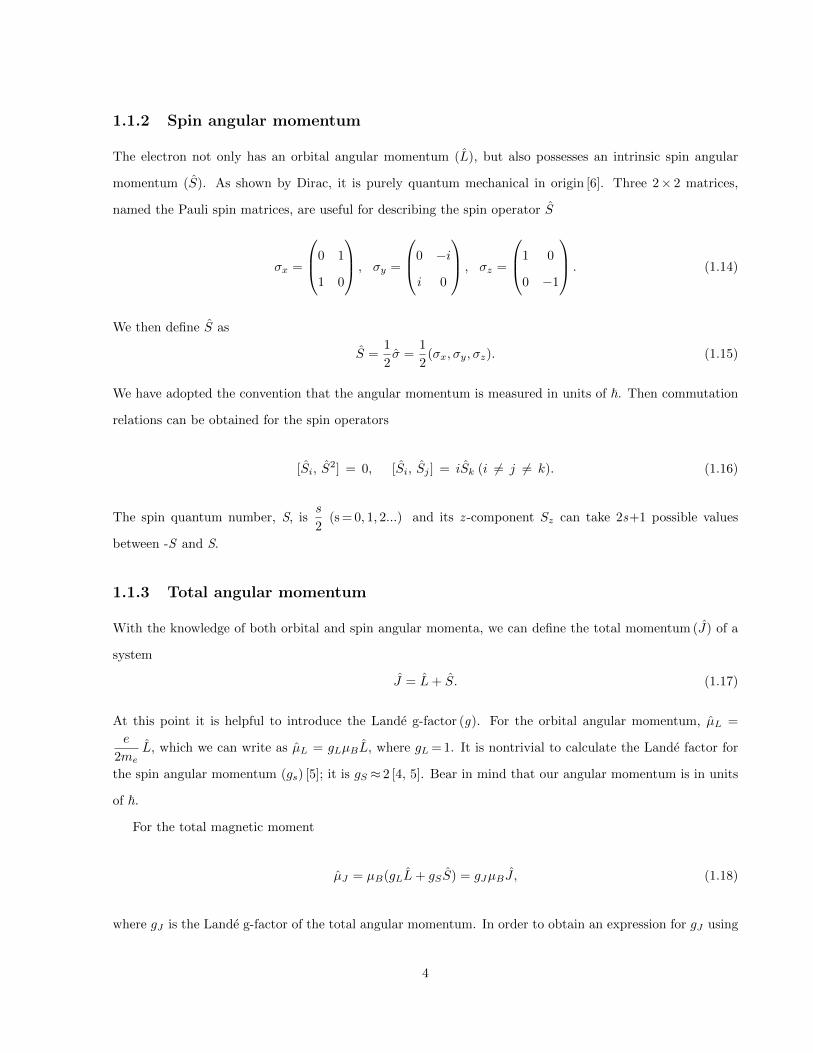
1.1.2 Spin angular momentum
The electron not only has an orbital angular momentum (L), but also possesses an intrinsic spin angular
momentum (S). As shown by Dirac, it is purely quantum mechanical in origin [6]. Three 2× 2 matrices,
named the Pauli spin matrices, are useful for describing the spin operator S
σx =
0 1
1 0
, σy =
0 −i
i 0
, σz =
1 0
0 −1
. (1.14)
We then define S as
S =1
2σ =
1
2(σx, σy, σz). (1.15)
We have adopted the convention that the angular momentum is measured in units of ~. Then commutation
relations can be obtained for the spin operators
[Si, S2] = 0, [Si, Sj ] = iSk (i 6= j 6= k). (1.16)
The spin quantum number, S, iss
2(s = 0, 1, 2...) and its z -component Sz can take 2s+1 possible values
between -S and S.
1.1.3 Total angular momentum
With the knowledge of both orbital and spin angular momenta, we can define the total momentum (J) of a
system
J = L+ S. (1.17)
At this point it is helpful to introduce the Lande g-factor (g). For the orbital angular momentum, µL =
e
2meL, which we can write as µL = gLµBL, where gL = 1. It is nontrivial to calculate the Lande factor for
the spin angular momentum (gs) [5]; it is gS ≈ 2 [4, 5]. Bear in mind that our angular momentum is in units
of ~.
For the total magnetic moment
µJ = µB(gLL+ gSS) = gJµB J , (1.18)
where gJ is the Lande g-factor of the total angular momentum. In order to obtain an expression for gJ using
4
gL, gS , J, L and S (J, L and S are eigenvalues of J , L and S), we mutiply both sides of eq. 1.18 by J
µB(gLL · J + gSS · J) = gJµB J2. (1.19)
And by inserting the following known expressions into eq. 1.19,
J2 = J(J + 1), L2 = L(L+ 1), S2 = S(S + 1), (1.20)
L · J =1
2(J2 + L2 − S2), (1.21)
S · J =1
2(J2 − L2 + S2), (1.22)
we obtain the Lande g-factor for the total angular momentum
gJ = gLJ(J + 1) + L(L+ 1)− S(S + 1)
2J(J + 1)+ gS
J(J + 1)− L(L+ 1) + S(S + 1)
2J(J + 1). (1.23)
Experimentally, we always measure the eigenvalues of J2 and Jz. As a result, we define two very important
parameters: the effective magnetic moment (Meff ) and the saturation moment along the field direction (Ms)
Meff = gJµB√J(J + 1), Ms = gJJµB . (1.24)
1.1.4 Paramagnetism
A material is expected to be paramagnetic in one of two conditions:
(i) the spins are well isolated in space so that the interaction energy between each pair (Ei) of spins is
negligible;
(ii) the thermal fluctuation energy (kBT, kB ≈ 8.617 × 10⁻⁵ eV K−1 is the Boltzmann constant) overwhelms
Ei.
In both cases, Ei is insignificant to the spin orientations. However, a non-zero magnetic moment will be
induced by applying a magnetic field. The energy of the electron with total angular momentum J is gJmµBB
(m = −J, −J + 1, ..., J − 1, J). As a result, the partition function is
Z =J∑
m=−Jexp(gJmµBB/kBT ). (1.25)
5
So the mean value of the total magnetic angular momentum m is
< m >=
J∑m=−J
m × exp(gJmµBB/kBT )
J∑m=−J
exp(gJmµBB/kBT )
. (1.26)
The magnetization of a system with n free spins can be determined by
M = ngJµB < m > . (1.27)
By writing y = gJµBJB/kBT and Ms = ngJJµB , we finally obtain
M = Ms2J + 1
2Jcoth(
2J + 1
2Jy)− 1
2Jcoth(
y
2J), (1.28)
where the BJ(y) =2J + 1
2Jcoth(
2J + 1
2Jy)− 1
2Jcoth(
y
2J) is the Brillouin function [4].
In the small y region (y 1, often corresponding to low magnetic field and not very low temperatures),
the susceptibility is expressed by
χ =M
H≈ µ0M
B=nµ0M
2eff
3kBT, (1.29)
using the Maclaurin expansion of coth (y). As a result, χ∝ 1/T and one can extract Meff (eq. 1.24) by
measuring χ in the paramagnetic region.
6

1.1.5 Crystal fields
Figure 1.2: (a) MO6-octahedron. M = TM ion (black solid). Oxygens are red solids. The orthogonal axes
are also labelled. (b) Crystal field splitting of the d orbitals.
For the 3d TM ion oxides, another important feature to consider is the local crystal environment due to the
exposed d orbitals. This effect is much weaker for 4f rare earth ions in which the 4f orbitals are well shielded
by the 5s and 5p outer shells. In the compounds investigated in this thesis, such crystal fields originate from
the overlap between the d orbitals of TM ions (e.g. Mn3+, Mn4+, Cr3+, Co2+) and the p oxygen orbitals. For
example, when an 3d TM ion is placed on the center of an octahedron where oxygens occupy the vertices
(Fig. 1.2a), the degeneracy of the d orbital will be lifted (Fig. 1.2b).
As shown in Fig. 1.1, the lobes of the dxy, dxz and dyz orbitals (called t2g orbitals) all point along the
diagonal directions between the x, y and z axes. However, the dz2 and dx2−y2 orbitals (called eg orbitals)
have their lobes lying along the main axes. Since the neighbouring 2p oxygen orbitals are also pointing
along the three main axes (Fig. 1.1), the eg orbitals will have a stronger electrostatic energy produced by
the electrons in the 2p oxygen orbitals. As a result, the five level d orbitals split into two groups, with the
three-fold t2g orbitals lying underneath the two-fold eg orbitals (Fig. 1.2b). The calculation of the energy gap
(∆oct) between the two levels can be found in Ref. [7]
It is also worth mentioning the empirical Hund’s rules which are used to predict the electron filling se-
quence in the d orbitals if they are not fully occupied [4]. They are arranged in decreasing importance:
1. The configuration with lowest energy is also the configuration with maximum S.
2. When (1) is fullfilled, the next step to lower the energy is to maximize L.
7
3. J = |L - S| if the shell is less than half filled, otherwise J = |L + S|.
These rules work very well for predicting the electronic configuration of 4f ions. In contrast, big discrepancies
may occur for 3d TM ions due to the presence of the crystal field [4]. Indeed, even the first of Hund’s rules
may be ignored if the crystal field is strong enough [8]. Moreover, Hund’s rules match the experiment much
better if one assumes that the orbital quantum number L = 0 [4]. This effect is called orbital quenching and
prevails in many TM oxides. However, non-zero angular momentum states can be introduced in systems
where the spin-orbit coupling is nonnegligible, e.g, α-CoV2O6 [9].
1.1.6 Jahn-Teller distortion
Figure 1.3: (upper) A Jahn-Teller distortion (elongation) for the MO6-octahedron. (bottom) The degeneracy
lifting after the distortion. The energy is lowered because the dz2 level is lowered. The energy saving for
lowering the dxz and dyz levels is balanced by the energy raising of the dxy level [4].
In a TMO6-octahedral environment, deviation of oxygen ions from their equilibrium positions is usually not
favoured. An increase in the energy, proportional to the square of the distortion, will be introduced [4, 2].
However, this motion may also lower the energy by lifting the orbital degeneracy of the central TM ion.
The resulting lattice change is called a Jahn-Teller (JT) distortion. As discussed in the last section, the
five-fold degeneracy of the 3d orbitals can be lifted by the crystal field effect to form eg (two-fold) and t2g
(three-fold) levels. When a JT effect happens, these levels may be further split [4]. This is achieved by
changing the overlap between the 3d TM orbitals and the 2p oxygen orbitals. Consequently, the energy of
certain orbitals is raised, while for the others’ it is lowered. Fig. 1.3 corresponds to the case of ‘elongation‘
8

along the z -axis. For the Mn3+ ion (3d4), the four electrons singly occupy the dyz, dxz, dxy and dz2 orbitals,
respectively. The JT distortion thus lowers the total energy related to these occupied d orbitals. When
placed into a lattice arrangement, such TMO6-octahedral distortion may become cooperative [2, 10]. As
will be demonstrated in this thesis, the cooperative JT distortion is crucial to understand various emergent
properties in mixed-valence perovskite manganites.
1.2 Interactions
1.2.1 Coulomb interactions
In a multiple orbital system, we can write the kinetic energy of the electrons as
Hkin =∑
~j,~j′,γ,γ′,σ
tγγ′
~j~j′c†~jγσc~j′γ′σ, (1.30)
where ~j is the site occupied by magnetic ions, γ and σ label the orbital and spin states, respectively [2]. The
Coulomb potential is
HC =1
2
∑~j
∑γ1γ2γ′
1γ′2
∑σ1σ2σ′
1σ′2
< γ1σ1, γ2σ2 || γ′1σ′1, γ′2σ′2 > c†~jγ1σ1c†~jγ2σ2
c~jγ′2σ
′2c~jγ′
1σ′1. (1.31)
In solid-state physics, an electron’s state (σ, γ,~j) can be described by the Wannier function, φγ σ (~j), which
is composed of a complete set of orthogonal functions [11]. Following this approach, the matrix element in
eq. 1.31 can be given by [10]
< γ1σ1, γ2σ2 || γ′1σ′1, γ′2σ′2 >=
∫ ∫d~jd~j′φ∗γ1σ1
(~j)φ∗γ2σ2(~j′)g~j−~j′φγ′
1σ′1(~j)φγ′
2σ′2(~j′). (1.32)
As a result, the Hamiltonian for a general problem is H = Hkin + HC . However, it is very difficult to exactly
solve these complicated interactions. Alternatively, eq. 1.31 can be replaced by an effective Hamiltonian
consisting of several parts as long as they can capture the essential underlying physics. For the 3d TM ions
investigated in this thesis, we have already shown that the five-fold orbitals split into eg and t2g levels due
to the crystal field effect. In many systems, e.g. manganese oxides, the t2g spins are very localized and less
affected by external perturbations. They can be treated as a ‘core-spin’ S~j so that the Coulomb coupling
between electron(s) in the eg (si) and t2g orbitals in one TM ion may be described by a Hund’s coupling
9
term
HHund = −JH∑i
siS~j . (1.33)
Another term Hel−el is required to account for the remaining Coulomb interactions between eg electrons [2,
10].
1.2.2 Exchange interactions
In the non-interacting limit, two indistinguishable electrons can be separately described by a spatial wave
function ψi (r) (i = a, b) [5]. One can use these functions to construct the spatial wave functions (Φ) of an
interacting two-electron system. Considering the exchange symmetry of Fermions as well as the spin part of
the wave function [5], there are two possible forms for Φ
Φ1 =1√2
[ψa (r1)ψb (r2) + ψa (r2)ψb (r1)]χs, (1.34)
Φ2 =1√2
[ψa (r1)ψb (r2)− ψa (r2)ψb (r1)]χt, (1.35)
where χs (χt) represents the singlet S = 0 (triplet S = 1) spin state [5]. Given the Hamiltonian (H) of the
system, one can also calculate the energy difference of the two possible states
∆E = E1 − E2 = 2
∫φ∗a (r1)φ∗b (r2)Hφ∗a (r2)φ∗b (r1)dr1dr2. (1.36)
If ∆ E is negative (positive), a singlet (triplet) state is favoured, corresponding to two spins antiparallel (parallel)
to each other. We can also construct an effective Hamiltonian (Heff ) using the following procedures
S2tot = (S1 + S2)2 = S2
1 + S22 + 2S1S2. (1.37)
Since Stot = 0, 1 and S1,S2 = 1/2, we obtain
S1S2 =1
4(triplet) or − 3
4(singlet). (1.38)
Finally, Heff can be written as
Heff =1
4(E1 + 3E2)− (E1 − E2)S1S2. (1.39)
10
The spin part of Heff is called the exchange interaction
Hex = −2JS1S2, (1.40)
where J =E1 − E2
2is the exchange constant. The main origin of such exchange interactions in solids is the
electron-electron Coulomb repulsions [4, 5].
For the many-body systems, there is an interaction between each pair of spins. It is very useful to
introduce the isotropic Heisenberg model
H = −∑ij
JijSiSj , (1.41)
where Jij is the exchange constant between each pair of spins. This model can be reduced to a XY-model if
the exchange is two-dimensional and an Ising-model if the exchange is one-dimensional [1]. Considering only
the nearest neighbour exchange, the relative alignment of the two neighbouring spins is determined by the
sign of the exchange constant.
If the wavefunctions of two neighbouring magnetic ions are sufficiently overlapping, a direct exchange
interaction is expected to set in. However, this term is usually less important in determining the magnetic
ground state in oxides because the corresponding magnetic ions are well separated in space. Thus indirect
exchange interactions must be taken into account.
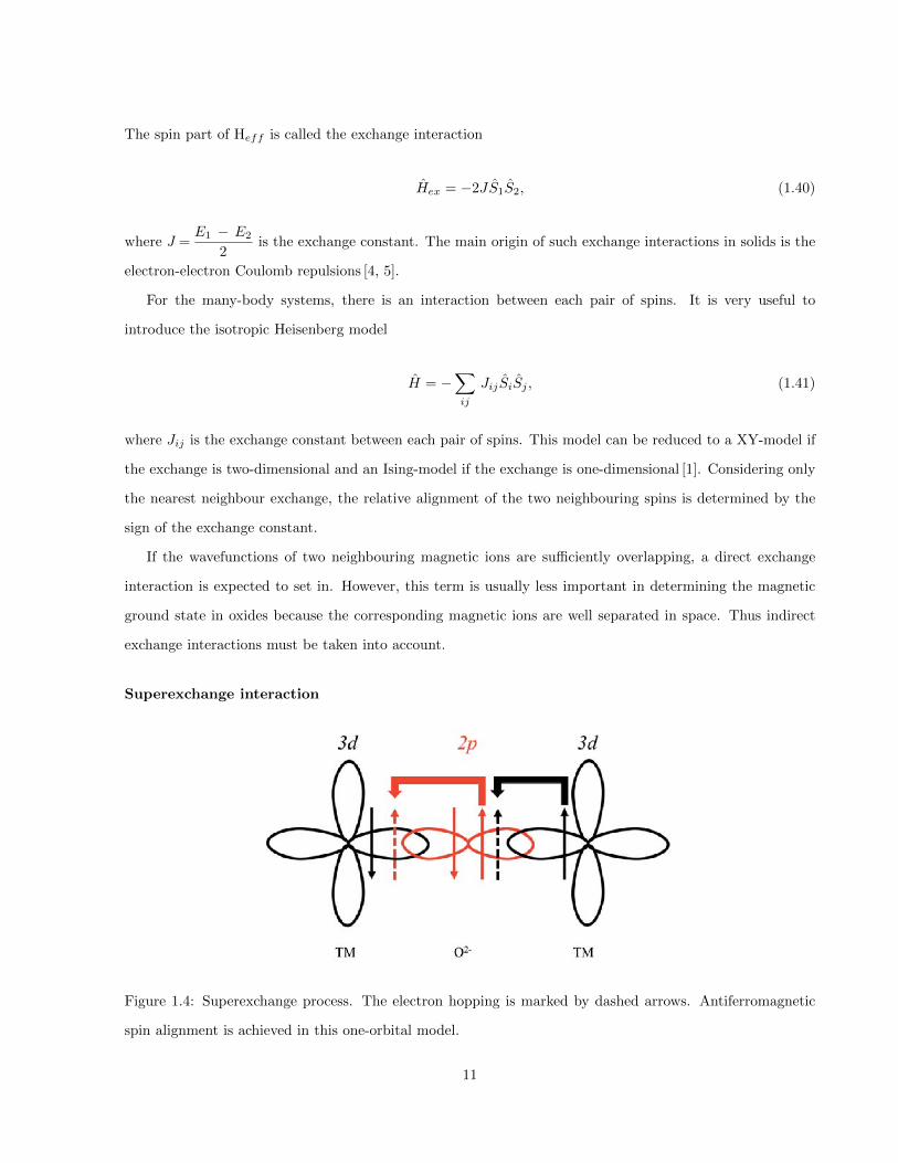
Superexchange interaction
Figure 1.4: Superexchange process. The electron hopping is marked by dashed arrows. Antiferromagnetic
spin alignment is achieved in this one-orbital model.
11
Superexchange is one type of indirect exchange which prevails in magnetic oxides. The nonmagnetic ion O2−
acts as an intermediary between the two magnetic ions. To simplify the physical process of superexchange,
we assume the 2p oxygen orbital overlaps with the same d orbital on each side of it (Fig. 1.4), and that
there is only one unpaired electron on the magnetic ion. To lower the kinetic energy of the system, this
electron tends to hop to the oxygen site. To accommodate this change, the 2p electron with the same spin
direction will hop into the d orbital of the other magnetic ion. Since this orbital is already singly occupied,
the new electron has to adopt the opposite spin direction due to the Pauli exclusion principle, resulting in
an antiferromagnetic alignment between the neighbouring spins (Fig. 1.4).
In practice, the overlap of orbitals (p, d) is much more complicated. Depending on the TM-O bond
length and the TM-O-TM bond angle, the magnetic exchange can even vary from antiferromagnetic to
ferromagnetic. A set of empirical rules, called the Goodenough-Kanamori rules, are helpful for determining
the correct magnetic order in many oxides [12]. For example, the superexchange between two magnetic ions
with partially filled d shells is strongly antiferromagnetic if the TM-O-TM bond angle is 180, whereas a 90
superexchange interaction is ferromagnetic and much weaker. Further information can be found in Ref. [12].
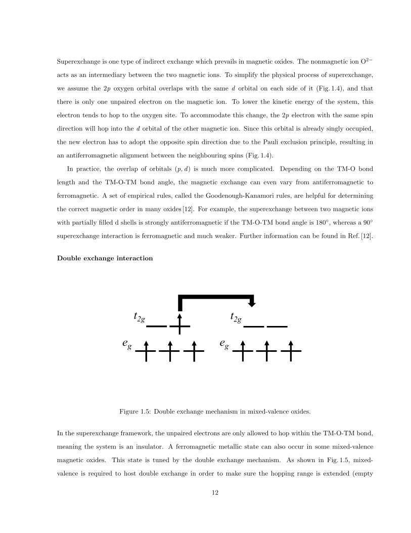
Double exchange interaction
Figure 1.5: Double exchange mechanism in mixed-valence oxides.
In the superexchange framework, the unpaired electrons are only allowed to hop within the TM-O-TM bond,
meaning the system is an insulator. A ferromagnetic metallic state can also occur in some mixed-valence
magnetic oxides. This state is tuned by the double exchange mechanism. As shown in Fig. 1.5, mixed-
valence is required to host double exchange in order to make sure the hopping range is extended (empty
12
orbitals), otherwise the superexchange mechanism will be recovered. Secondly, ferromagnetic alignment of
the neighbouring spins is favoured since the strong Hund’s couping from the core spins in the t2g orbitals
will try to align the eg spin along them. The double exchange mechanism can qualitatively explain the
charge transport properties in mixed-valence systems such as Fe3O4 and La1−xSrxMnO3, though not in a
comprehensive way [10, 13].
1.2.3 Dzyaloshinsky-Moriya interaction
If the centre of the bond connecting two spins does not contain inversion symmetry, the anisotropic exchange
interaction Dzyaloshinsky-Moria (DM) interaction is allowed [14]. It is the higher order correction of the
Dirac equation and couples the exicted state of one ion and the ground state of the other [4]. It takes the
form
HDM = Dij · Si × Sj , (1.42)
where ~Dij is a vector and its direction depends on the symmetry [14]. The DM interaction can play a
significant role in pyrochlore lattices [15], as the geometry permits a non-zero DM term.
1.2.4 Magnetic dipolar interaction
The long range interaction between two magnetic dipoles with magnetc moments ~J1, ~J2 separated by ~r can
be expressed by
Hdip =µ0
4πr3[ ~J1 · ~J2 −
3
r2( ~J1 · ~r)( ~J2 · ~r)]. (1.43)
This term is small (a few Kelvin) and therefore not important at high temperatures. However, for those
oxides where the magnetism comes from rare earth ions with very large magnetic moments, the dipolar
interaction still needs to be considered [4, 15].
1.2.5 Spin-orbit coupling
Although spin-orbit coupling is a relativistic effect in origin, it can be phenomenologically understood using
a classical model [4]. In the electron reference frame, the motion of the electron orbiting can be alternatively
viewed as the motion of nucleus. As a result, an additional magnetic field term exists,
~B =~ε × ~v
c2, (1.44)
13

where ~ε = −~δ ~V (~r), v is the orbiting velocity and ~V (~r) is the potential energy of the electron. As mentioned
above, this magnetic field will interact with the electron spin (m) in the form of
HSO = −1
2m · B =
e~2
2mec2r
dV (r)
drS · L, (1.45)
where ~L = me~r×~v and e = (ge~/2m)S [4]. Since most orbital wave functions (e.g. p, d) have aspherical dis-
tributions (Fig. 1.1), the spin-orbit coupling is responsible for the magnetocrystalline (single-ion) anisotropy
(Han) in materials.
1.2.6 Electron-phonon coupling
Figure 1.6: Two eg-active JT modes.
For a TMO6-octahedron, there are 7 (number of ions)× 3 (three dimensional motion) = 21 JT modes in total
to consider. Since we shall focus on mixed-valence manganese oxides in this thesis, only 2 modes, usually
written as Q2 and Q3, are important to the eg orbital splitting of Mn3+ [2]. These two modes are depicted
in Fig. 1.6. The potential change of an electron related to the JT distortion, assuming the presence of both
modes is
∆VJT =2√
6
21
9
a4< r2 >
[Q2
0 1
1 0
+Q3
1 0
0 −1
], (1.46)
where r and a are the electron - Mn3+ and oxygen - Mn3+ distance, respectively [2]. We replace the matrices
in this equation by the Pauli symbols in eq. 1.14. Then we can express the total energy by including the
14
energy penalization caused by distortion itself
H = −g(Q2σx +Q3σz) +1
2Mω2[Q2
2 +Q23], (1.47)
where g = -(2√
6/21) 9a4 < r2 >. Finally, by applying the second-quantization process and summing over all
sites (i = 1, 2, 3...), the electron-phonon coupling term of the system is
Hel−ph =∑i
−[2g(Q2iT
xi +Q3iT
zi ) + (kJT /2)(Q2
2i +Q23i)], (1.48)
where kJT =Mω2 and T x,y,zi are pseudospin operators [2]. In theoretical calculations, the dimensionless
parameter λ = g/√kJT t (t is the hopping amplitude in eq. 1.30) is used to characterize the electron-phonon
coupling strength [10].
1.2.7 Ruderman-Kittel-Kasuya-Yosida interaction
The exchange between localized magnetic ions in metals is mediated by the conducting electrons. This type
of indirect exchange is known as the Ruderman-Kittel-Kasuya-Yosida (RKKY) interaction [4, 16, 17, 18]. Its
Hamiltonian takes the form of
HRKKY (r) ∝ cos(2kF r)
r3, (1.49)
where r is the distance between two localized magnetic ions, and kF is the radius of the Fermi surface which
is assumed to be spherical [4]. The key feature revealed by eq. 1.49 is that the RKKY interaction is long
range in nature with its sign oscillating as a function of r.
1.3 Frustrated magnetism
1.3.1 Geometric frustration
In addition to the competing interactions, sometimes referred as ‘random frustration’ in the literature [15],
‘geometric frustration’ also plays an important role on determining the magnetic structure in relevant systems.
As shown in Fig. 1.7a, when the antiferromagnetically coupled spins are assigned to occupy the corners
of the triangular (tetrahedral) lattice, the antiparallel configuration between each pair of spins cannot be
achieved simultaneously. This effect is called ’geometric frustration‘. A pyrochlore lattice (A2B2O7) has a
cubic crystallographic structure (space group Fd-3m) and consists of two sets of corner-sharing tetrahedral
15
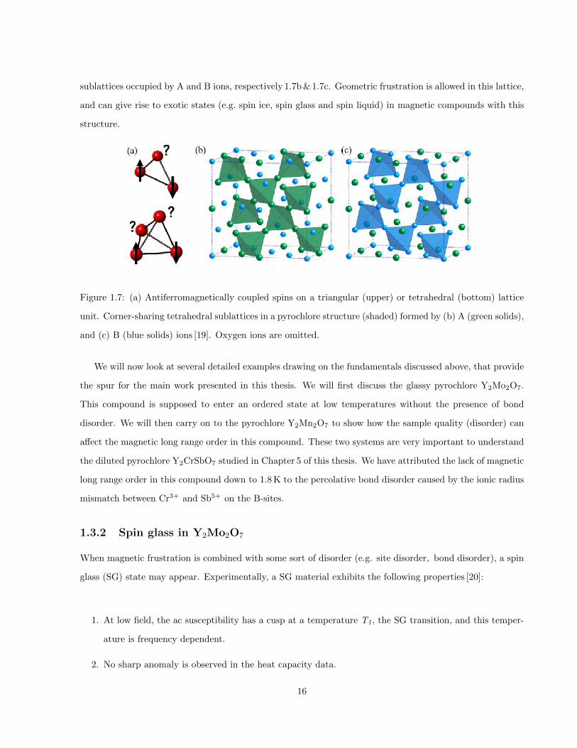
sublattices occupied by A and B ions, respectively 1.7b & 1.7c. Geometric frustration is allowed in this lattice,
and can give rise to exotic states (e.g. spin ice, spin glass and spin liquid) in magnetic compounds with this
structure.
Figure 1.7: (a) Antiferromagnetically coupled spins on a triangular (upper) or tetrahedral (bottom) lattice
unit. Corner-sharing tetrahedral sublattices in a pyrochlore structure (shaded) formed by (b) A (green solids),
and (c) B (blue solids) ions [19]. Oxygen ions are omitted.
We will now look at several detailed examples drawing on the fundamentals discussed above, that provide
the spur for the main work presented in this thesis. We will first discuss the glassy pyrochlore Y2Mo2O7.
This compound is supposed to enter an ordered state at low temperatures without the presence of bond
disorder. We will then carry on to the pyrochlore Y2Mn2O7 to show how the sample quality (disorder) can
affect the magnetic long range order in this compound. These two systems are very important to understand
the diluted pyrochlore Y2CrSbO7 studied in Chapter 5 of this thesis. We have attributed the lack of magnetic
long range order in this compound down to 1.8 K to the percolative bond disorder caused by the ionic radius
mismatch between Cr3+ and Sb5+ on the B-sites.
1.3.2 Spin glass in Y2Mo2O7
When magnetic frustration is combined with some sort of disorder (e.g. site disorder, bond disorder), a spin
glass (SG) state may appear. Experimentally, a SG material exhibits the following properties [20]:
1. At low field, the ac susceptibility has a cusp at a temperature T f , the SG transition, and this temper-
ature is frequency dependent.
2. No sharp anomaly is observed in the heat capacity data.
16
3. The susceptibility is history dependent below T f , i.e. the zero-field-cooled (ZFC) and field-cooled (FC)
data diverge below T f .
4. Magnetization decays with time below T f
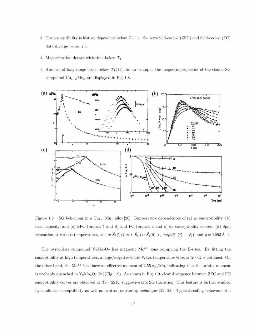
5. Absence of long range order below T f [15]. As an example, the magnetic properties of the classic SG
compound Cu1−xMnx are displayed in Fig. 1.8.
Figure 1.8: SG behaviour in a Cu1−xMnx alloy [20]. Temperature dependences of (a) ac susceptibility, (b)
heat capacity, and (c) ZFC (branch b and d) and FC (branch a and c) dc susceptibility curves. (d) Spin
relaxation at various temperatures, where ~S(~q, t) ∝< ~Si(t) · ~Sj(0) >T exp[i~q · (~ri − ~rj)] and q = 0.093 A−1.
The pyrochlore compound Y2Mo2O7 has magnetic Mo4+ ions occupying the B-sites. By fitting the
susceptibility at high temperatures, a large/negative Curie-Weiss temperature ΘCW' -200 K is obtained. On
the other hand, the Mo4+ ions have an effective moment of 2.55µB/Mo, indicating that the orbital moment
is probably quenched in Y2Mo2O7 [21] (Fig. 1.9). As shown in Fig. 1.9, clear divergence between ZFC and FC
susceptibility curves are observed at T f = 22 K, suggestive of a SG transition. This feature is further studied
by nonlinear susceptibility as well as neutron scattering techniques [22, 23]. Typical scaling behavour of a
17

SG is observed near to T f (Fig. 1.9). Moreover, quasielastic spin excitations are detected above T f . At low
temperatures, these fluctuations are replaced by a static short range order with correlation length less than
5 A (Fig. 1.10).
Figure 1.9: (Left) Inverse susceptibililty versus temperature (solids) curve of Y2Mo2O7. The black line is a
linear fit to its high temperature part [21]. (Top right) ZFC and FC curves when B = 0.01 T [23]. (Bottom
right) Nonlinear susceptibility χnl analyzed according to the critical scaling model in Ref. [23]
Based on the experimental evidence provided above, the SG state in Y2Mo2O7 is well established. How-
ever, the driving mechanism of this state has still not been fully understood yet. In general, magnetic
frustration and disorder are the building blocks for a SG state. For example, the spin exchange in the
Cu1−xMnx alloy is of the RKKY type, the sign of which is very sensitive to the distance between the two
magnetic sites (eq. 1.49) [20]. The SG state in this compound is caused by the site disorder of Mn. Several
investigations, including extended X-ray-absorption fine structure (EXAFS) and nuclear magnetic resonance
(NMR) and neutron pair distribution function (PDF), have been carried out to characterize the local disorder
level in Y2Mo2O7 [24, 25, 26]. These results reveal: (i) discrete lattice distortions which may suppress the
magnetic frustration [26], and (ii) very weak bond length fluctuations (6 5 % for Mo-Mo bond)[24]. Never-
18

theless, such a disorder level is too low to induce a SG state according to the conventional mean field theory
predictions [27].
Figure 1.10: (Left) Low energy inelastic neutron spectrum of Y2Mo2O7 at different temperatures [22].
(Right) Elastic magnetic structure factor S(Q) versus scattering vector (Q) plot at 1.4 K [22].
An alternative approach of modelling a pyrochlore spin lattice with bond disorder is to start from the
classical Heisenberg antiferromagnet in eq. 1.41, where the ground state is highly degenerate [15, 28]. Bond
disorder produces exchange fluctuations ~∆ to the original average exchange constant ~J . Saunders et al
treat ~∆ as a perturbation to the ground state degeneracy in the weak disorder limit (| ~∆ | | ~J |) [29]. By
parametrizing the ground states in terms of a gauge field, they project ~∆ into the nearest neighbour exchange
interactions so that effective long range interactions are generated [29]. Using Monte Carlo simulations, a
SG transition at a finite temperature T f is found. However, the predicted T f only scales with | ~∆ | and is
much smaller than the experimentally determined value in Y2Mo2O7 (∼ 22 K) [29, 23]. In order to correctly
reproduce T f , an additional spin-lattice coupling term is required, as revealed in Ref. [30]. Finally, we note
the origin of spin-lattice coupling in Y2Mo2O7 may be related to the orbital frustration according to the
latest X-ray and neutron PDF investigations as well as density functional theory (DFT) calculations [31, 32].
19

1.3.3 Long range order in Y2Mn2O7
Figure 1.11: Heat capacity data measured by Reimers et al [33] (a) and Shimakwa et al [34] (b). (c)
ZFC and FC magnetization versus temperature curves at B = 0.15 mT (circle), 0.56 mT(square) and 10 mT
(triangle) [33]. (d) Magnetization versus magnetic field curves at various temperaures. From top to bottom:
1.8 K, 5 K, 7.5 K, 10 K, 15 K, 20 K, 25 K, 30 K, 35 K, 40 K, 45 K, 50 K [33]. (e) Real and imaginary parts of
the ac susceptibility. The inset shows the frequency dependence at low temperatures [33].
To the best of our knowledge, the magnetic structure of Y2Mn2O7 is still a mystery. Earlier studies by
Reimer et al [33] did not show any transition in the heat capacity data. Instead, typical magnetic properties
belonging to a SG, e.g. frequency dependence of ac susceptibility, divergence between ZFC and FC curves,
were observed (Fig. 1.11). The SG scenario is further supported by small angle neutron scattering measure-
ments (Fig. 1.12) [35]. In addition to the Lorentzian term which describes the conventional ferromagnetic
spin-spin correlations, a Lorentzian-squared term is required to fit the neutron intensity as a function of
scattering vector Q
I (Q) =A
(Q2 + 1/ξ21)+
B
(Q2 + 1/ξ22)2, (1.50)
where the second term is used to characterize the random field in the sample [35]. From the temperature
dependence of ξ1 in Fig. 1.12, it is clear that true long range ferromagnetic order is never reached [35].
20

Since rare earth manganese pyrochlores cannot be grown at ambient pressure, these compounds must
be synthesized using high pressure methods [15]. Another explanation for the earlier observations is poor
sample quality. This would also explain the low saturation moment measured in high magnetic field on
those samples. Although it should be 3µB/Mn assuming the orbital moment is quenched, only 2µB/Mn was
reached at B = 4 T. In fact, weak ferromagnetism was observed in the neutron powder diffraction patterns at
7 K, which apparently contradicts the SG scenario [33]. Much better samples were produced by Shimakawa et
al [34], who have observed a λ-shape peak in the heat capacity measurements as well as 3µB/Mn saturation
moment at much lower field B = 2 T (Fig. 1.11b). Unfortunately, there has been no subsequent work on these
improved samples since then.
Figure 1.12: Small angle neutron scattering measurements on Y2Mn2O7 [35]. (Left) Neutron intensity versus
scattering vector Q at different temperatures (solids). The solid and dotted lines are the numerical fits using
eq. 1.50 with and without the instrumental resolution function. (Right) Temperature dependences of the two
types of magnetic correlation length, ξ1 and ξ2.
1.4 Phase separation
The ground states of some systems tend to be intrinsically inhomogeneous due to the competition of multiple
interactions. This phenomenon is commonly described as ‘phase separation’. In this section, we will introduce
two types of phase separation compounds: (I) Ca3Co2O6 in which the phase separation is related to the
competing magnetic interactions, and (II) manganese perovskites in which the phase separation involves
nonmagnetic interactions, and spans from atomic to micrometre scales. In Chapter 3, we will present another
21
compound, γ-CoV2O6, in which the phase separation is also of magnetic origin. Unlike Ca3Co2O6 which
shows a dynamic phase separation effect, the phase separation of γ-CoV2O6 is static. In Chapter 4, we
will demonstrate how the phase separation in a strained manganese perovskite is coupled with the carrier
transport and magnetic order by varying the magnetic field.
1.4.1 Dynamic phase separation in Ca3Co2O6
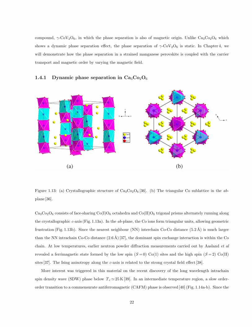
Figure 1.13: (a) Crystallographic structure of Ca3Co2O6 [36]. (b) The triangular Co sublattice in the ab-
plane [36].
Ca3Co2O6 consists of face-sharing Co(I)O6 octahedra and Co(II)O6 trigonal prisms alternately running along
the crystallographic c-axis (Fig. 1.13a). In the ab-plane, the Co ions form triangular units, allowing geometric
frustration (Fig. 1.13b). Since the nearest neighbour (NN) interchain Co-Co distance (5.2 A) is much larger
than the NN intrachain Co-Co distance (2.6 A) [37], the dominant spin exchange interaction is within the Co
chain. At low temperatures, earlier neutron powder diffraction measurements carried out by Aasland et al
revealed a ferrimagnetic state formed by the low spin (S = 0) Co(1) sites and the high spin (S = 2) Co(II)
sites [37]. The Ising anisotropy along the c-axis is related to the strong crystal field effect [38].
More interest was triggered in this material on the recent discovery of the long wavelength intrachain
spin density wave (SDW) phase below T c' 25 K [39]. In an intermediate temperature region, a slow order-
order transition to a commensurate antiferromagnetic (CAFM) phase is observed [40] (Fig. 1.14a-b). Since the
22
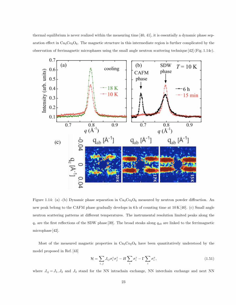
thermal equilibrium is never realized within the measuring time [40, 41], it is essentially a dynamic phase sep-
aration effect in Ca3Co2O6. The magnetic structure in this intermediate region is further complicated by the
observation of ferrimagnetic microphases using the small angle neutron scattering technique [42] (Fig. 1.14c).
Figure 1.14: (a) -(b) Dynamic phase separation in Ca3Co2O6 measured by neutron powder diffraction. An
new peak belong to the CAFM phase gradually develops in 6 h of counting time at 10 K [40]. (c) Small angle
neutron scattering patterns at different temperatures. The instrumental resolution limited peaks along the
qc are the first reflections of the SDW phase [39]. The broad steaks along qab are linked to the ferrimagnetic
microphase [42].
Most of the measured magnetic properties in Ca3Co2O6 have been quantitatively understood by the
model proposed in Ref. [43]
H =∑i, j
Jijσzi σ
zj −H
∑i
σzi − Γ∑i
σxi , (1.51)
where Jij = J1, J2 and J3 stand for the NN intrachain exchange, NN interchain exchange and next NN
23
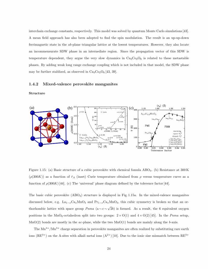
interchain exchange constants, respectively. This model was solved by quantum Monte Carlo simulations [43].
A mean field approach has also been adopted to find the spin modulation. The result is an up-up-down
ferrimagnetic state in the ab-plane triangular lattice at the lowest temperatures. However, they also locate
an incommensurate SDW phase in an internediate region. Since the propagation vector of this SDW is
temperature dependent, they argue the very slow dynamics in Ca3Co2O6 is related to these metastable
phases. By adding weak long range exchange coupling which is not included in that model, the SDW phase
may be further stablized, as observed in Ca3Co2O6 [43, 39].
1.4.2 Mixed-valence perovskite manganites
Structure
Figure 1.15: (a) Basic structure of a cubic perovskite with chemical fomula ABO3. (b) Resistance at 300 K
(ρ(300K)) as a function of rA (inset) Curie temperature obtained from ρ versus temperature curve as a
function of ρ(300K) [44]. (c) The ‘universal’ phase diagram defined by the tolerence factor [44].
The basic cubic perovskite (ABO3) structure is displayed in Fig. 1.15a. In the mixed-valence manganites
discussed below, e.g. La1−xCaxMnO3 and Pr1−xCaxMnO3, this cubic symmetry is broken so that an or-
thorhombic lattice with space group Pnma (a∼ c∼√
2b) is formed. As a result, the 6 equivalent oxygen
positions in the MnO6-octahedron split into two groups: 2×O(1) and 4×O(2) [45]. In the Pnma setup,
MnO(2) bonds are mostly in the ac-plane, while the two MnO(1) bonds are mainly along the b-axis.
The Mn4+/Mn3+ charge separation in perovskite manganites are often realized by substituting rare earth
ions (RE3+) on the A-sites with alkali metal ions (A2+) [10]. Due to the ionic size mismatch between RE3+
24
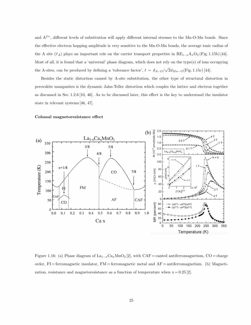
and A2+, different levels of substitution will apply different internal stresses to the Mn-O-Mn bonds. Since
the effective electron hopping amplitude is very sensitive to the Mn-O-Mn bonds, the average ionic radius of
the A site (rA) plays an important role on the carrier transport properties in RE1−xAxO3 (Fig. 1.15b) [44].
Most of all, it is found that a ‘universal’ phase diagram, which does not rely on the type(s) of ions occupying
the A-sites, can be produced by defining a ‘tolerance factor’, t = dA−O/√
2dMn−O(Fig. 1.15c) [44].
Besides the static distortion caused by A-site substitution, the other type of structural distortion in
perovskite manganites is the dynamic Jahn-Teller distortion which couples the lattice and electron together
as discussed in Sec. 1.2.6 [10, 46]. As to be discussed later, this effect is the key to understand the insulator
state in relevant systems [46, 47].
Colossal magnetoresistance effect
Figure 1.16: (a) Phase diagram of La1−xCaxMnO3 [2], with CAF = canted antiferromagnetism, CO = charge
order, FI = ferromagnetic insulator, FM = ferromagnetic metal and AF = antiferromagnetism. (b) Magneti-
zation, resistance and magnetoresistance as a function of temperature when x = 0.25 [2].
25
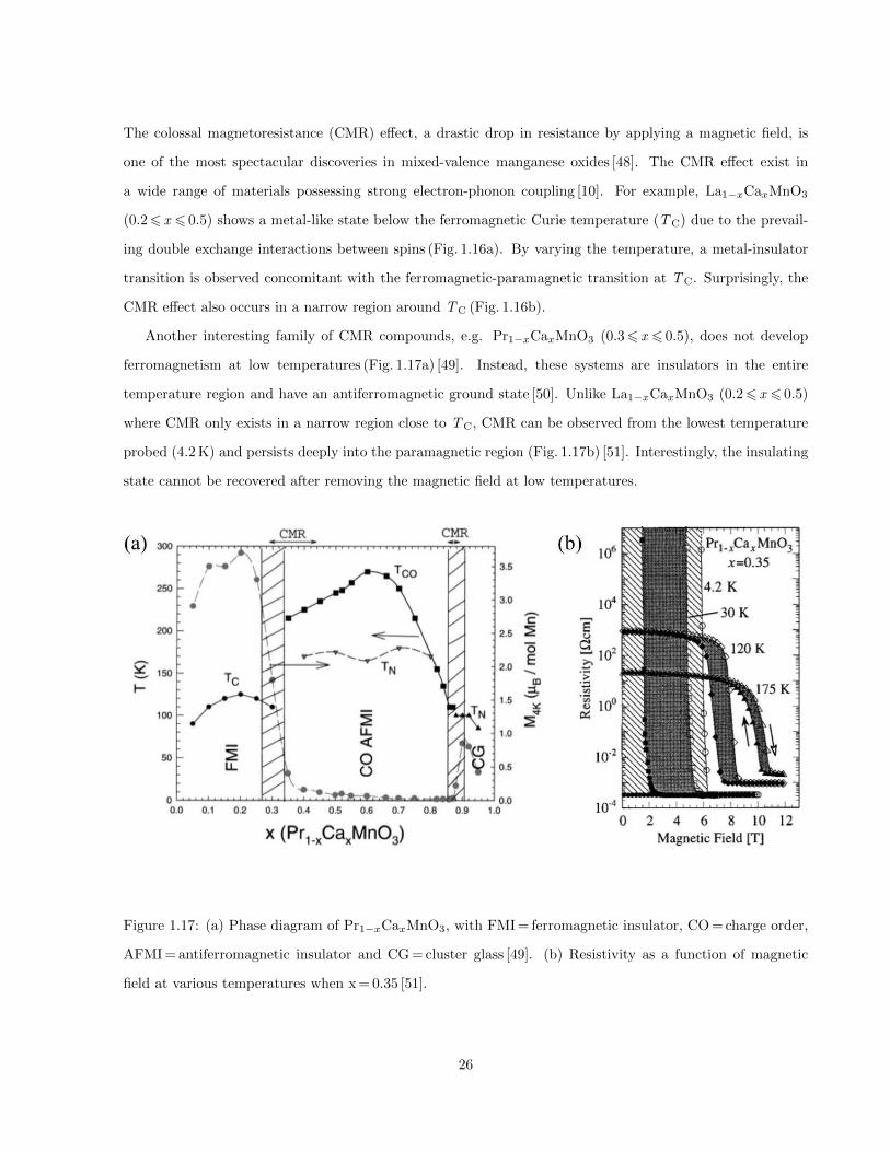
The colossal magnetoresistance (CMR) effect, a drastic drop in resistance by applying a magnetic field, is
one of the most spectacular discoveries in mixed-valence manganese oxides [48]. The CMR effect exist in
a wide range of materials possessing strong electron-phonon coupling [10]. For example, La1−xCaxMnO3
(0.26 x 6 0.5) shows a metal-like state below the ferromagnetic Curie temperature (TC) due to the prevail-
ing double exchange interactions between spins (Fig. 1.16a). By varying the temperature, a metal-insulator
transition is observed concomitant with the ferromagnetic-paramagnetic transition at TC. Surprisingly, the
CMR effect also occurs in a narrow region around TC (Fig. 1.16b).
Another interesting family of CMR compounds, e.g. Pr1−xCaxMnO3 (0.36 x 6 0.5), does not develop
ferromagnetism at low temperatures (Fig. 1.17a) [49]. Instead, these systems are insulators in the entire
temperature region and have an antiferromagnetic ground state [50]. Unlike La1−xCaxMnO3 (0.26 x 6 0.5)
where CMR only exists in a narrow region close to TC, CMR can be observed from the lowest temperature
probed (4.2 K) and persists deeply into the paramagnetic region (Fig. 1.17b) [51]. Interestingly, the insulating
state cannot be recovered after removing the magnetic field at low temperatures.
Figure 1.17: (a) Phase diagram of Pr1−xCaxMnO3, with FMI = ferromagnetic insulator, CO = charge order,
AFMI = antiferromagnetic insulator and CG = cluster glass [49]. (b) Resistivity as a function of magnetic
field at various temperatures when x = 0.35 [51].
26

Spin, charge and orbital order
Figure 1.18: d3x2−r2/d3y2−r2 orbital order under Pbcm space group (a ' b'√
2c) setup [52]. The orbital
orientations of the Mn3+ ions are marked by the lobes. The black and red arrows show the spin arrangement
in the z = 0 plane. The spins in the z = 1/2 plane are reversed (unchanged) for the CE (pseudo-CE) type
antiferromagnetic order [50].
The magnetic order in CMR manganites couples tightly to the charge and orbital degrees of freedom [2].
Fig. 1.18 shows the d3x2−r2/d3y2−r2 orbital order which is commonly observed in Pr1−xCaxMnO3 (x > 0.3) [52].
Since only Mn3+ has an occupied eg orbital, orbital order is often accompanied by some sort of charge order.
The antiferromagnetic spin arrangement of Pr1−xCaxMnO3 in the ab-plane (space group Pbcm, a ' b'√
2c)
has also been shown in Fig. 1.18. And it is called charge-exchange (CE) or pseudo-CE type antiferromag-
netism, in which the spins in the ab-plane couple antiferromagnetically or ferromagnetically along the c-
axis [50].
27

Electronic phase separation and colossal magnetoresistance
Figure 1.19: (a)-(b) Resistivity versus temperature curves under different electron-phonon coupling strengths
λ with fixed n. Details of the density parameter n can be found in Ref. [47]. (c)-(d) Resistivity versus
temperature curves at various magnetic fields with fixed n [47]. (e) Temperature dependence of the standard
deviation of Mn-O bond lengths in La1−xCaxMnO3 measured by Booth et al. [53]. Clear softening of the
distortion is observed below TC.
Various models have been proposed to explain the electronic phase separation (e.g. polarons, charge order)
in mixed-valence manganese oxides [10, 54]. Here we will follow the treatments carried out by Millis et al
where the electron-phonon coupling is through the dynamic Jahn-Teller distortion [47]. First of all, we define
an effective Hamiltonian
Heff = Hkin + HHund + Hel−ph + HZeeman. (1.52)
These terms represent the kinetic energy (eq. 1.30), Hund’s intraband coupling (eq. 1.33), electron-phonon cou-
pling (eq. 1.48), and Zeeman energy (eq. 1.11), respectively. They have solved Heff by assuming HHund→∞.
When the electron-phonon coupling strength (characterized by λ = g/√kJT t (t in eq. 1.48) is strong enough,
a gap in the electron spectral function, corresponding to the formation of polarons, only opens above
TC (Fig. 1.19a & 1.19b). Most of all, the CMR effect can be reproduced by tuning the magnetic field in
HZeeman (Fig. 1.19c & 1.19d). The existence of a Jahn-Teller distortion in the CMR temperature region, e.g.
above TC in La1−xCaxMnO3 (0.26 x 6 0.5), has been confirmed using local probe techniques such as PDF
and EXAFS [53, 55, 46](Fig. 1.19e). Since not all of the Mn ions are Jahn-Teller active, the dynamic Jahn-
Teller distortion will lead to inhomogeneities on the atomic scales, i.e. electronic phase separation [10]. The
28
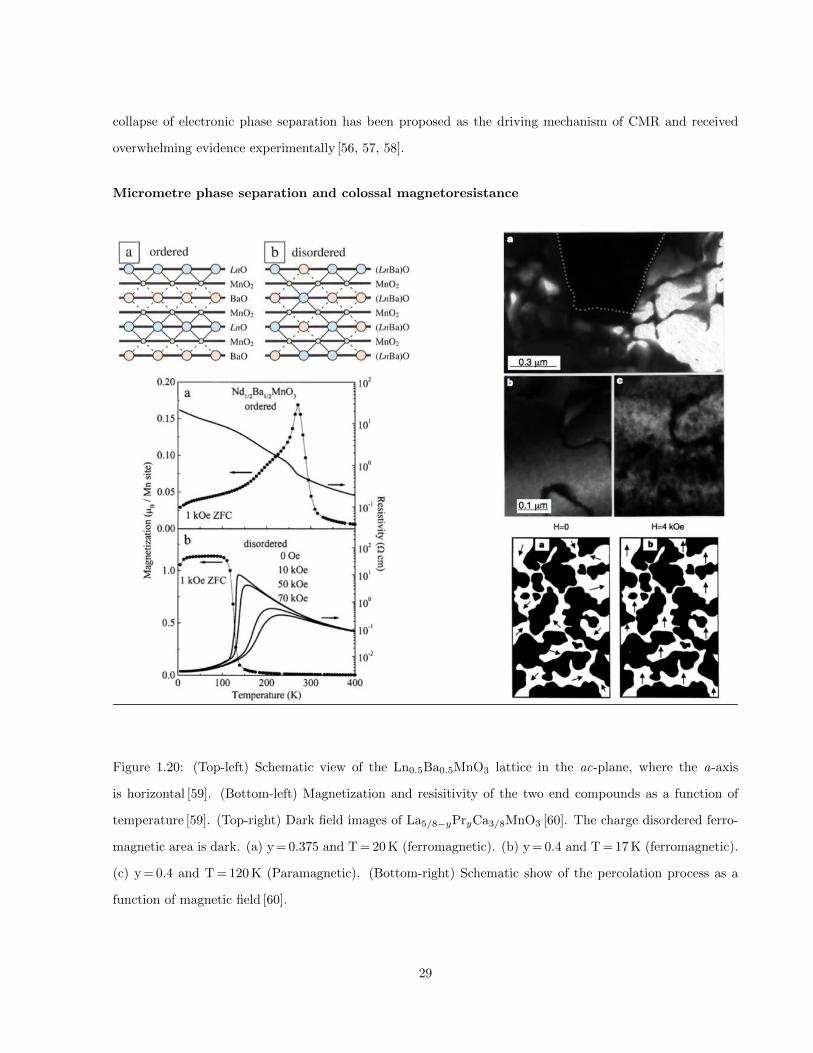
collapse of electronic phase separation has been proposed as the driving mechanism of CMR and received
overwhelming evidence experimentally [56, 57, 58].
Micrometre phase separation and colossal magnetoresistance
Figure 1.20: (Top-left) Schematic view of the Ln0.5Ba0.5MnO3 lattice in the ac-plane, where the a-axis
is horizontal [59]. (Bottom-left) Magnetization and resisitivity of the two end compounds as a function of
temperature [59]. (Top-right) Dark field images of La5/8−yPryCa3/8MnO3 [60]. The charge disordered ferro-
magnetic area is dark. (a) y = 0.375 and T = 20 K (ferromagnetic). (b) y = 0.4 and T = 17 K (ferromagnetic).
(c) y = 0.4 and T = 120 K (Paramagnetic). (Bottom-right) Schematic show of the percolation process as a
function of magnetic field [60].
29
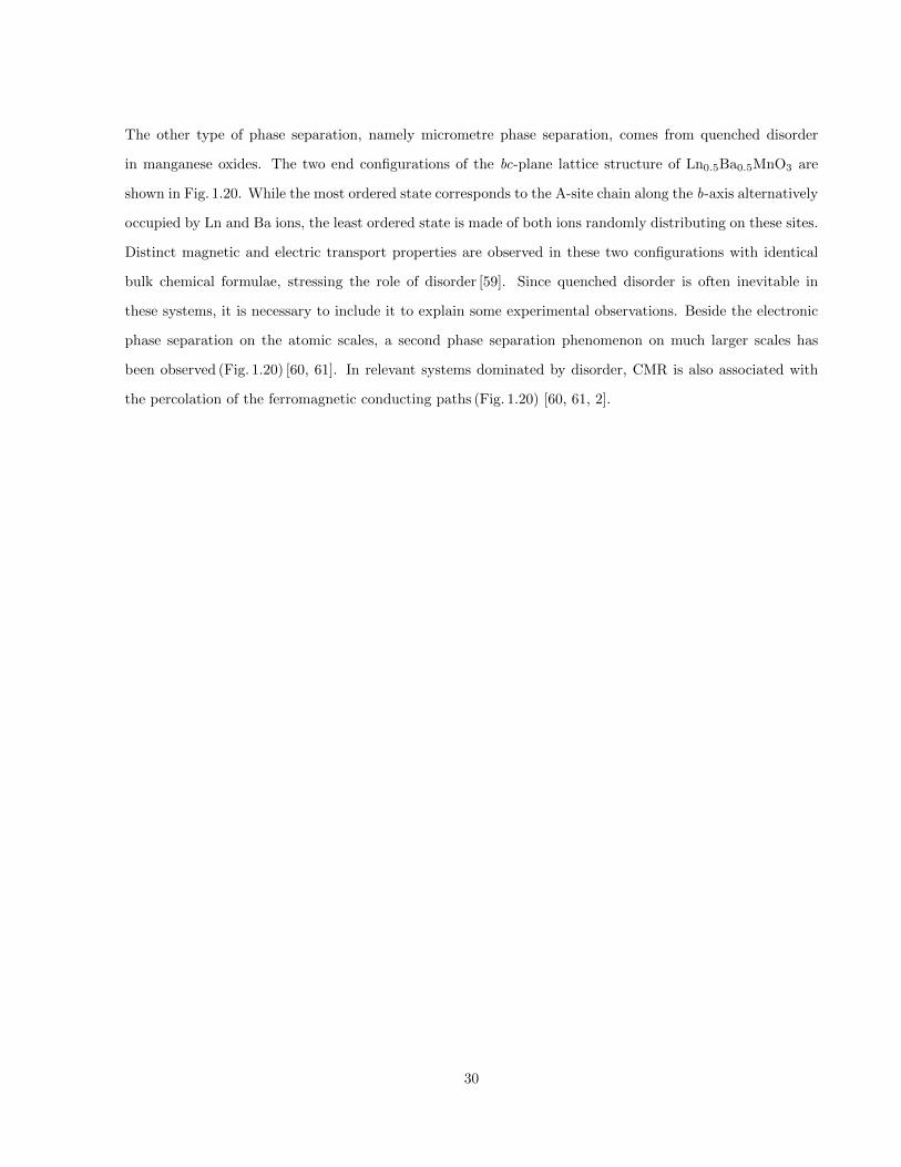
The other type of phase separation, namely micrometre phase separation, comes from quenched disorder
in manganese oxides. The two end configurations of the bc-plane lattice structure of Ln0.5Ba0.5MnO3 are
shown in Fig. 1.20. While the most ordered state corresponds to the A-site chain along the b-axis alternatively
occupied by Ln and Ba ions, the least ordered state is made of both ions randomly distributing on these sites.
Distinct magnetic and electric transport properties are observed in these two configurations with identical
bulk chemical formulae, stressing the role of disorder [59]. Since quenched disorder is often inevitable in
these systems, it is necessary to include it to explain some experimental observations. Beside the electronic
phase separation on the atomic scales, a second phase separation phenomenon on much larger scales has
been observed (Fig. 1.20) [60, 61]. In relevant systems dominated by disorder, CMR is also associated with
the percolation of the ferromagnetic conducting paths (Fig. 1.20) [60, 61, 2].
30

CHAPTER 2
EXPERIMENTAL TECHNIQUES
2.1 Sample synthesis
Several polycrystalline samples were prepared for this thesis using the ceramic method [62]. The detailed syn-
thesis procedures are provided in the corresponding chapters. In general, this method contains the following
steps:
1. High purity raw metal oxides in the correct stoichiometric proportions are ground together using an
agate pestle and mortar.
2. The resulting homogeneous mixture is then pressed into a pellet by applying hydrostatic pressure in
order to reduce the empty space between particles.
3. The pellet is heated in a furnace to trigger the solid state reaction.
A solid state reaction is realized by the diffusion of ions in the raw mixture. Since these ions need sufficient
energy to break and reform chemical bonds as well as migrate over long atomic distances, these reactions are
slow and require high temperatures [62].
2.2 Scattering techniques
The majority of the experimental work discussed in this thesis was done using a variety of scattering tech-
niques, described below. First, however, we look at some basic concepts in scattering theory.
31

2.2.1 Basic scattering theory
As a beam of particles characterized by the wavevector ~ki hits a target, those particles will be scattered to
form a certain distribution in space and time (Fig. 2.1). Such a distribution can be described in terms of a
quantity known as the cross-section (σ). We can set up a detector a distance D from the target to measure
the number of particles scattered in a given direction (θ,φ) and energy (E ). If D the dimensions of the
detector and the target, we can define the partial differential cross-sectiond2σ
dΩ dE, where the solid angle
dΩ = sinθdθdφ [63]. If the scattering process is elastic (|~ki|= |~kf | in Fig. 2.1), we will be only measuring the
differential cross-sectiondσ
dΩ; this quantity is the focus in this thesis.
Figure 2.1: Geometry for a scattering process.
In a typical neutron (X-ray) scattering process, the wavelength (∼ 10−10 m) of the incident particles is
much larger than the effective range (∼ 10−14 m) of the interaction between the particle and target. As a
result, the scattered wave is independent of φ [63]. If the scattering process only involves a single target with
fixed position, the scattered wavefunction at the point of r may be written as
ψf =f (θ, λ)
rexp(ikr). (2.1)
In reality, we are measuring a crystal consisting of a large number of atoms occupying crystallographic sites
32
labelled as Rj (j = 1, 2...). Eq. 2.1 therefore needs to be modified to
ψf = exp(i~kf · ~r)∑j
fj (θ, λ)exp(i ~Q · ~Rj)|~r − ~Rj |
, (2.2)
where ~Q=~ki -~kf . When counting the number of of neutrons N (θ, λ) with wavelength λ scattered in the
direction of θ, the distance between the detector and target (r) is always much larger than the size of the
sample. This means we can use the approximation |~r - ~Rj |= r. N (θ, λ) deflected into a small area δS of the
detector is then related to |ψf |2 by
N(θ, λ) ∝ δS∣∣∣∑j
fj (θ, λ)exp(i ~Q · ~Rj)
r
∣∣∣2 = δΩ|Fhkl|2, (2.3)
where hkl are the Miller indices and Fhkl is the structure factor. If the system contains a large number of
crystals with random orientations, i.e. in a powder form, the measured intensity can be expressed as [64, 63,
65]
I = I0r2e
1 + cos22θ
2
1
16π rLλ3|Fhkl|2n
1
V 2c
DVp, (2.4)
where I0 is the intensity per unit area of the incident beam, r2e = 7.9× 10⁻²⁶ cm2 (re is called the Thomson
scattering length),1 + cos22θ
2is the polarization factor, L is the Lorentz factor which depends on the
experimental configuration, n is the multiplicity of the hkl -lattice plane, Vc is the volume of a unit cell, D is
the temperature (Debye-Waller) factor and Vp is the total volume of the powder. A detailed discussion on
these parameters can be found in Ref. [64, 63, 65]
33
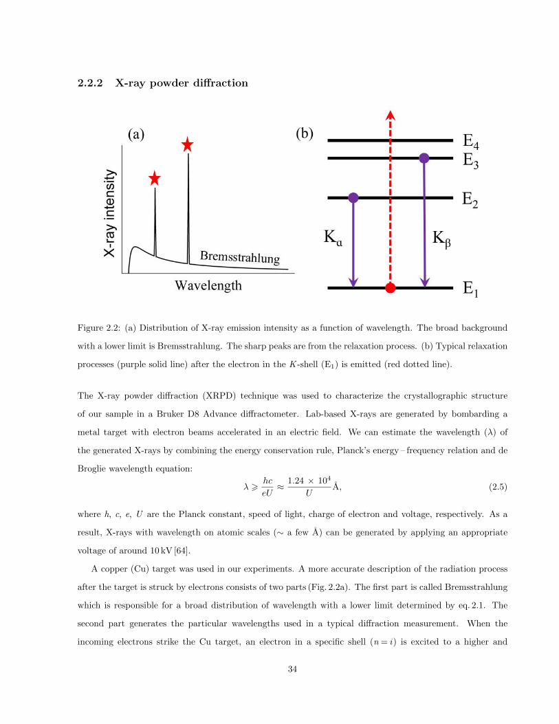
2.2.2 X-ray powder diffraction
Figure 2.2: (a) Distribution of X-ray emission intensity as a function of wavelength. The broad background
with a lower limit is Bremsstrahlung. The sharp peaks are from the relaxation process. (b) Typical relaxation
processes (purple solid line) after the electron in the K -shell (E1) is emitted (red dotted line).
The X-ray powder diffraction (XRPD) technique was used to characterize the crystallographic structure
of our sample in a Bruker D8 Advance diffractometer. Lab-based X-rays are generated by bombarding a
metal target with electron beams accelerated in an electric field. We can estimate the wavelength (λ) of
the generated X-rays by combining the energy conservation rule, Planck’s energy – frequency relation and de
Broglie wavelength equation:
λ >hc
eU≈ 1.24 × 10⁴
UA, (2.5)
where h, c, e, U are the Planck constant, speed of light, charge of electron and voltage, respectively. As a
result, X-rays with wavelength on atomic scales (∼ a few A) can be generated by applying an appropriate
voltage of around 10 kV [64].
A copper (Cu) target was used in our experiments. A more accurate description of the radiation process
after the target is struck by electrons consists of two parts (Fig. 2.2a). The first part is called Bremsstrahlung
which is responsible for a broad distribution of wavelength with a lower limit determined by eq. 2.1. The
second part generates the particular wavelengths used in a typical diffraction measurement. When the
incoming electrons strike the Cu target, an electron in a specific shell (n = i) is excited to a higher and
34

unoccupied state, leaving this shell empty. This is followed by the relaxation of another electron from a
higher energy shell (n = j, j > i) to this low energy and empty shell (n = i), as well as the emission of a
photon with a wavelength
λij =hc
Ej − Ei, (2.6)
where Ei and Ej are the energies of the denoted shells (Fig. 2.2b). The strongest emission isKα, corresponding
to i = 1 and j = 2. In practice, a filter or a crystal monochromator is used to remove the unwanted wavelengths.
We have used a curved germanium crystal monochromator to select only the CuKα1 line (λ= 1.5406 A).
For the crystallographic structure determination, it is very important to understand the term f (θ, λ)
which is called the atomic form factor (eq. 2.1 - eq. 2.4). In a X-ray scattering case, this term can be writen
as
f (θ, λ) = Zg(Q)re, (2.7)
where Z is the atomic number and Q =4π sinθ
λis the wavevector transfer in eq. 2.2. Analytical approxima-
tions to g(Q) can be found in Ref. [66].
35
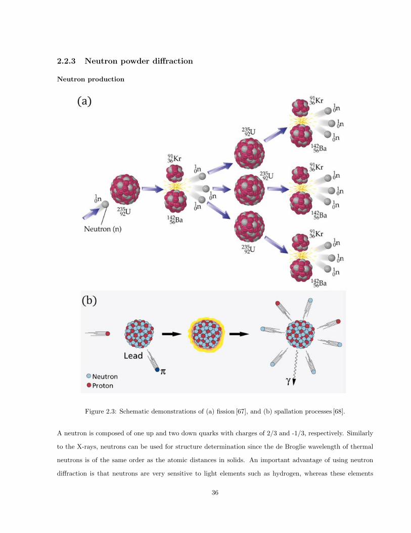
2.2.3 Neutron powder diffraction
Neutron production
Figure 2.3: Schematic demonstrations of (a) fission [67], and (b) spallation processes [68].
A neutron is composed of one up and two down quarks with charges of 2/3 and -1/3, respectively. Similarly
to the X-rays, neutrons can be used for structure determination since the de Broglie wavelength of thermal
neutrons is of the same order as the atomic distances in solids. An important advantage of using neutron
diffraction is that neutrons are very sensitive to light elements such as hydrogen, whereas these elements
36
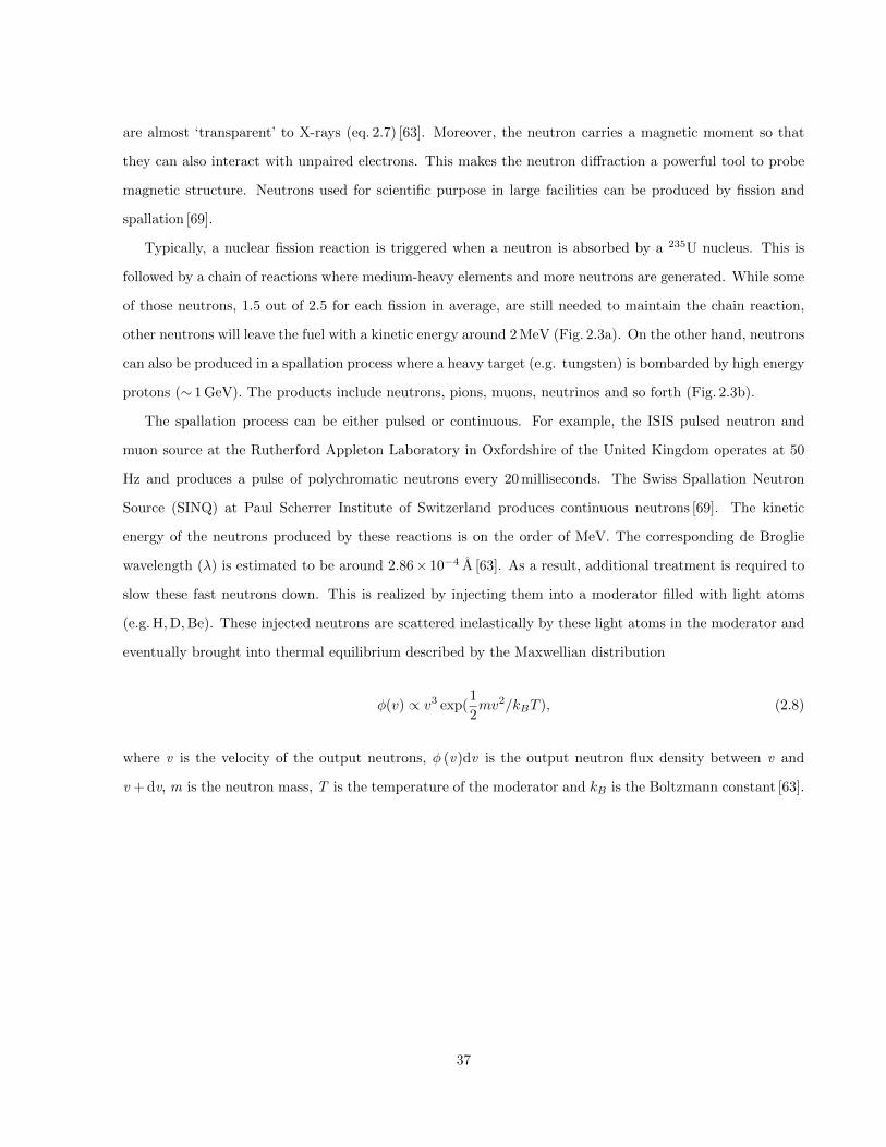
are almost ‘transparent’ to X-rays (eq. 2.7) [63]. Moreover, the neutron carries a magnetic moment so that
they can also interact with unpaired electrons. This makes the neutron diffraction a powerful tool to probe
magnetic structure. Neutrons used for scientific purpose in large facilities can be produced by fission and
spallation [69].
Typically, a nuclear fission reaction is triggered when a neutron is absorbed by a 235U nucleus. This is
followed by a chain of reactions where medium-heavy elements and more neutrons are generated. While some
of those neutrons, 1.5 out of 2.5 for each fission in average, are still needed to maintain the chain reaction,
other neutrons will leave the fuel with a kinetic energy around 2 MeV (Fig. 2.3a). On the other hand, neutrons
can also be produced in a spallation process where a heavy target (e.g. tungsten) is bombarded by high energy
protons (∼ 1 GeV). The products include neutrons, pions, muons, neutrinos and so forth (Fig. 2.3b).
The spallation process can be either pulsed or continuous. For example, the ISIS pulsed neutron and
muon source at the Rutherford Appleton Laboratory in Oxfordshire of the United Kingdom operates at 50
Hz and produces a pulse of polychromatic neutrons every 20 milliseconds. The Swiss Spallation Neutron
Source (SINQ) at Paul Scherrer Institute of Switzerland produces continuous neutrons [69]. The kinetic
energy of the neutrons produced by these reactions is on the order of MeV. The corresponding de Broglie
wavelength (λ) is estimated to be around 2.86× 10⁻⁴ A [63]. As a result, additional treatment is required to
slow these fast neutrons down. This is realized by injecting them into a moderator filled with light atoms
(e.g. H, D, Be). These injected neutrons are scattered inelastically by these light atoms in the moderator and
eventually brought into thermal equilibrium described by the Maxwellian distribution
φ(v) ∝ v3 exp(1
2mv2/kBT ), (2.8)
where v is the velocity of the output neutrons, φ (v)dv is the output neutron flux density between v and
v + dv, m is the neutron mass, T is the temperature of the moderator and kB is the Boltzmann constant [63].
37
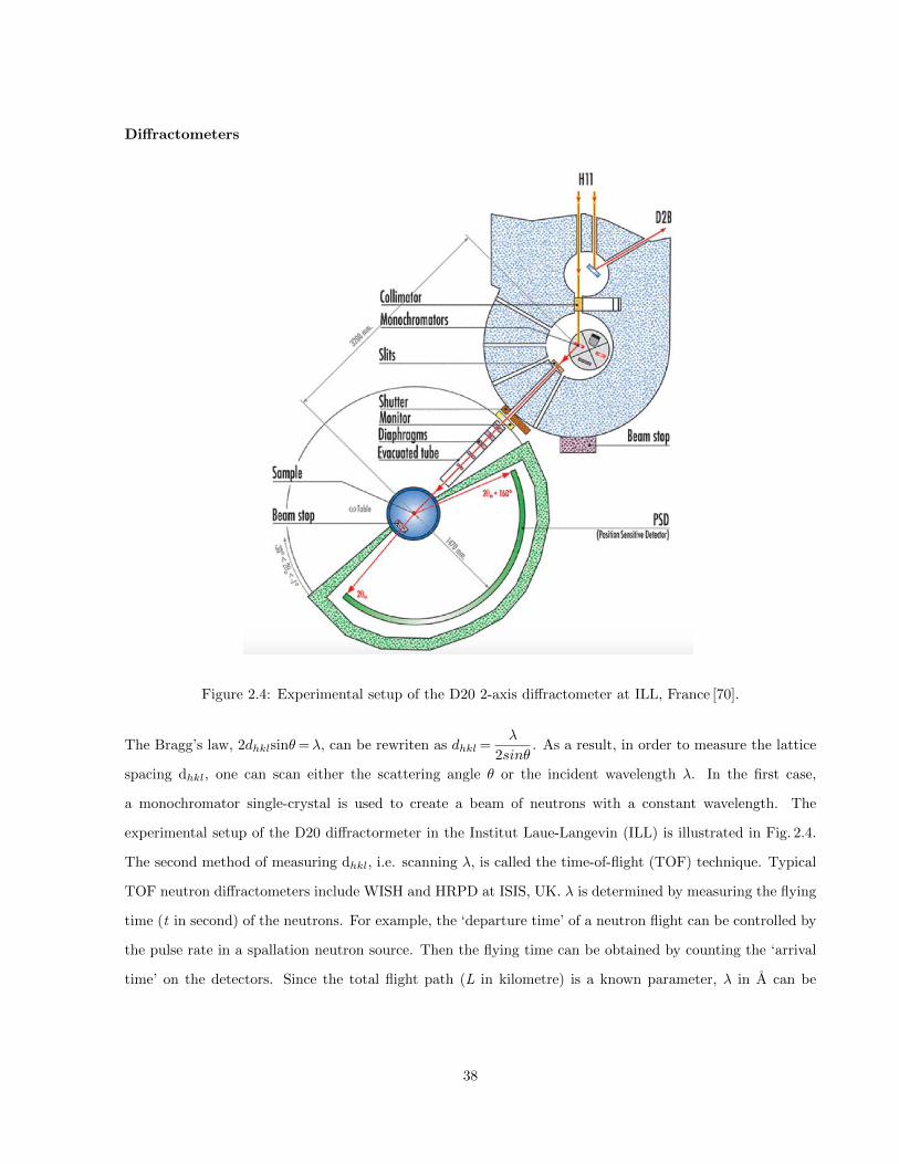
Diffractometers
Figure 2.4: Experimental setup of the D20 2-axis diffractometer at ILL, France [70].
The Bragg’s law, 2dhklsinθ=λ, can be rewriten as dhkl =λ
2sinθ. As a result, in order to measure the lattice
spacing dhkl, one can scan either the scattering angle θ or the incident wavelength λ. In the first case,
a monochromator single-crystal is used to create a beam of neutrons with a constant wavelength. The
experimental setup of the D20 diffractormeter in the Institut Laue-Langevin (ILL) is illustrated in Fig. 2.4.
The second method of measuring dhkl, i.e. scanning λ, is called the time-of-flight (TOF) technique. Typical
TOF neutron diffractometers include WISH and HRPD at ISIS, UK. λ is determined by measuring the flying
time (t in second) of the neutrons. For example, the ‘departure time’ of a neutron flight can be controlled by
the pulse rate in a spallation neutron source. Then the flying time can be obtained by counting the ‘arrival
time’ on the detectors. Since the total flight path (L in kilometre) is a known parameter, λ in A can be
38

obtained by [63]
λ = 3.956t
L. (2.9)
Nuclear scattering length b
Figure 2.5: Coherent nuclear scattering length b as a function of atomic number Z [71].
In most neutron scattering processes which do not involve magnetic interactions, f (θ, λ) in eq. 2.1 - eq. 2.4
can be replaced by a simple constant -b called ‘scattering length’ (Fig. 2.5). Compared with the atomic form
factor in the X-ray scattering case, the scattering length -b [64]
1. is invariant with respect to θ and λ.
2. is isotope sensitive.
3. has two different values for nuclei with a non-zero spin.
4. does not vary with atomic number Z in a trivial or monotonic way.
Magnetic form factor
As mentioned above, neutrons also carry a magnetic dipole moment which can interact with the magnetic
field produced by the unpaired electrons. When a neutron is scattered with a wavevector ~Q=~ki -~kf , it is
only sensitive to the magnetic moment ( ~M) perpendicular to ~Q: M⊥= ~M - ( ~M · ~Q) ~Q [63, 64]. The magnetic
39
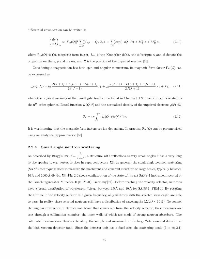
differential cross-section can be writen as
(dσ
dΩ
)m
∝ |Fm(Q)|2∑α, β
(δαβ − ~Qα ~Qβ) ×∑R
exp(−i ~Q · ~R) < Mα0 >< Mβ
R >, (2.10)
where Fm(Q) is the magnetic form factor, δαβ is the Kronecker delta, the subscripts α and β denote the
projection on the x, y and z axes, and R is the position of the unpaired electron [63].
Considering a magnetic ion has both spin and angular momentum, its magnetic form factor Fm(Q) can
be expressed as
gJFm(Q) = gLJ(J + 1) + L(L+ 1)− S(S + 1)
2J(J + 1)F0 + gS
J(J + 1)− L(L+ 1) + S(S + 1)
2J(J + 1)(F0 + F2), (2.11)
where the physical meaning of the Lande g-factors can be found in Chapter 1.1.3. The term Fn is related to
the nth order spherical Bessel function jn( ~Q ·~r) and the normalised density of the unpaired electrons ρ(~r) [63]
Fn = 4π
∫ ∞0
jn( ~Q · ~r)ρ(~r)r2dr. (2.12)
It is worth noting that the magnetic form factors are ion-dependent. In practise, Fm(Q) can be parametrized
using an analytical approximation [66].
2.2.4 Small angle neutron scattering
As described by Bragg’s law, d =λ
2sinθ, a structure with reflections at very small angles θ has a very long
lattice spacing d, e.g. vortex lattices in superconductors [72]. In general, the small angle neutron scattering
(SANS) technique is used to measure the incoherent and coherent structure on large scales, typically between
10 A and 1000 A[69, 64, 73]. Fig. 2.6 shows configuration of the state-of-the-art SANS-1 instrument located at
the Forschungsreaktor Munchen II (FRM-II), Germany [74]. Before reaching the velocity selector, neutrons
have a broad distribution of wavelength (λ)e.g. between 4.5 A and 30 A for SANS-1, FRM-II. By rotating
the turbine in the velocity selector at a given frequency, only neutrons with the selected wavelength are able
to pass. In reality, these selected neutrons still have a distribution of wavelengths (∆λ/λ∼ 10 %). To control
the angular divergence of the neutron beam that comes out from the velocity selector, these neutrons are
sent through a collimation chamber, the inner walls of which are made of strong neutron absorbers. The
collimated neutrons are then scattered by the sample and measured on the large 2-dimensional detector in
the high vacuum detector tank. Since the detector unit has a fixed size, the scattering angle (θ in eq. 2.1)
40
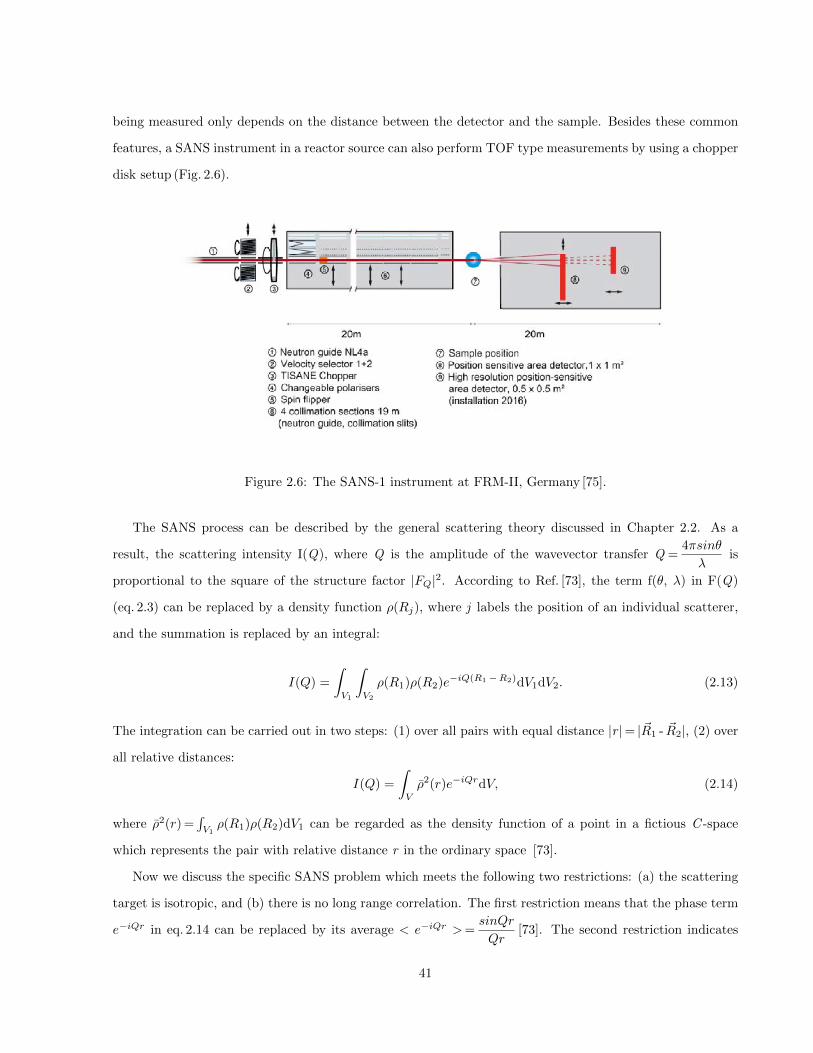
being measured only depends on the distance between the detector and the sample. Besides these common
features, a SANS instrument in a reactor source can also perform TOF type measurements by using a chopper
disk setup (Fig. 2.6).
Figure 2.6: The SANS-1 instrument at FRM-II, Germany [75].
The SANS process can be described by the general scattering theory discussed in Chapter 2.2. As a
result, the scattering intensity I(Q), where Q is the amplitude of the wavevector transfer Q =4πsinθ
λis
proportional to the square of the structure factor |FQ|2. According to Ref. [73], the term f(θ, λ) in F(Q)
(eq. 2.3) can be replaced by a density function ρ(Rj), where j labels the position of an individual scatterer,
and the summation is replaced by an integral:
I(Q) =
∫V1
∫V2
ρ(R1)ρ(R2)e−iQ(R1−R2)dV1dV2. (2.13)
The integration can be carried out in two steps: (1) over all pairs with equal distance |r |= |~R1 - ~R2|, (2) over
all relative distances:
I(Q) =
∫V
ρ2(r)e−iQrdV, (2.14)
where ρ2(r) =∫V1ρ(R1)ρ(R2)dV1 can be regarded as the density function of a point in a fictious C -space
which represents the pair with relative distance r in the ordinary space [73].
Now we discuss the specific SANS problem which meets the following two restrictions: (a) the scattering
target is isotropic, and (b) there is no long range correlation. The first restriction means that the phase term
e−iQr in eq. 2.14 can be replaced by its average < e−iQr >=sinQr
Qr[73]. The second restriction indicates
41

that the density functions of the pair separated widely enough in ordinary space should be independent so
that ρ2(r)→ a constant Vρ2 when r→∞ [73]. Since this constant term (background) does not contribute to
the intensity I(Q) based on eq. 2.14, it is the density fluctuation ∆ρ, also refered as the contrast term, in the
finite region that matters in a SANS process [73]. In other words, if the system is homogeneous on the scales
investigated by SANS, no relevant information can be probed. This makes the SANS technique an ideal tool
to study the phase separation phenomenon discussed in Chapter 1.4 [10].
2.3 Magnetometry
2.3.1 Magnetic Property Measurement System (MPMS)
The MPMS, manufactured by Quantum Design, can be used to measure the magnetization of a material. It
includes five principal components [76]:
1), Temperature control system.
2), Magnet control system.
3), Superconducting quantum interference device (SQUID).
4), Sample handling system.
5), Computer operating system.
Figure 2.7: (a) A SQUID is formed by two parallel Josephson junctions [77]. (b) Working mechanism of the
SQUID. Any weak change in the flux signal will be detected in the output voltage channel as well [77].
A SQUID is formed by two superconductors separated by thin insulating layers (Fig. 2.7a). This structure
has two parallel Josephson junctions which allow the tunelling of Cooper pairs [78]. Since the SQUID is
42
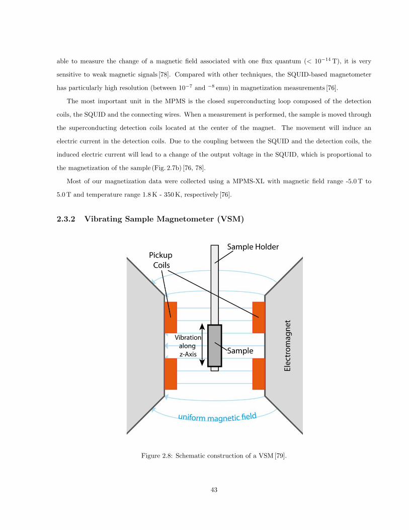
able to measure the change of a magnetic field associated with one flux quantum (< 10−14 T), it is very
sensitive to weak magnetic signals [78]. Compared with other techniques, the SQUID-based magnetometer
has particularly high resolution (between 10−7 and −8 emu) in magnetization measurements [76].
The most important unit in the MPMS is the closed superconducting loop composed of the detection
coils, the SQUID and the connecting wires. When a measurement is performed, the sample is moved through
the superconducting detection coils located at the center of the magnet. The movement will induce an
electric current in the detection coils. Due to the coupling between the SQUID and the detection coils, the
induced electric current will lead to a change of the output voltage in the SQUID, which is proportional to
the magnetization of the sample (Fig. 2.7b) [76, 78].
Most of our magnetization data were collected using a MPMS-XL with magnetic field range -5.0 T to
5.0 T and temperature range 1.8 K - 350 K, respectively [76].
2.3.2 Vibrating Sample Magnetometer (VSM)
Figure 2.8: Schematic construction of a VSM [79].
43
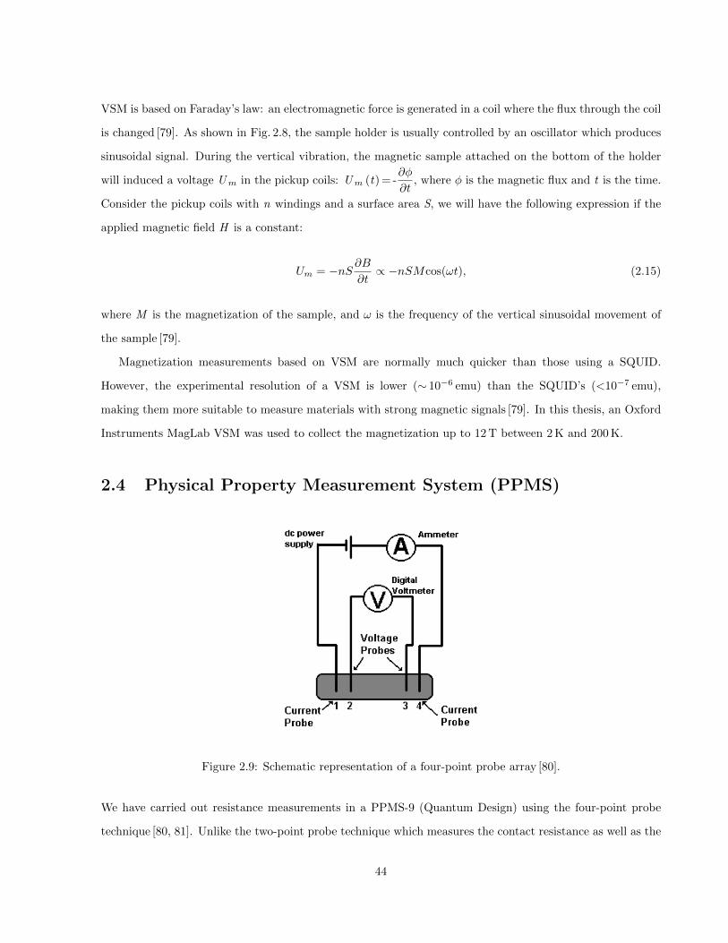
VSM is based on Faraday’s law: an electromagnetic force is generated in a coil where the flux through the coil
is changed [79]. As shown in Fig. 2.8, the sample holder is usually controlled by an oscillator which produces
sinusoidal signal. During the vertical vibration, the magnetic sample attached on the bottom of the holder
will induced a voltage Um in the pickup coils: Um (t) = -∂φ
∂t, where φ is the magnetic flux and t is the time.
Consider the pickup coils with n windings and a surface area S, we will have the following expression if the
applied magnetic field H is a constant:
Um = −nS ∂B∂t∝ −nSMcos(ωt), (2.15)
where M is the magnetization of the sample, and ω is the frequency of the vertical sinusoidal movement of
the sample [79].
Magnetization measurements based on VSM are normally much quicker than those using a SQUID.
However, the experimental resolution of a VSM is lower (∼ 10−6 emu) than the SQUID’s (<10−7 emu),
making them more suitable to measure materials with strong magnetic signals [79]. In this thesis, an Oxford
Instruments MagLab VSM was used to collect the magnetization up to 12 T between 2 K and 200 K.
2.4 Physical Property Measurement System (PPMS)
Figure 2.9: Schematic representation of a four-point probe array [80].
We have carried out resistance measurements in a PPMS-9 (Quantum Design) using the four-point probe
technique [80, 81]. Unlike the two-point probe technique which measures the contact resistance as well as the
44

intrinsic resistance of the sample, the four-point probe technique significantly reduces the contributions of
the contact resistance by separating the current injection from the voltage reading (Fig. 2.9).
45
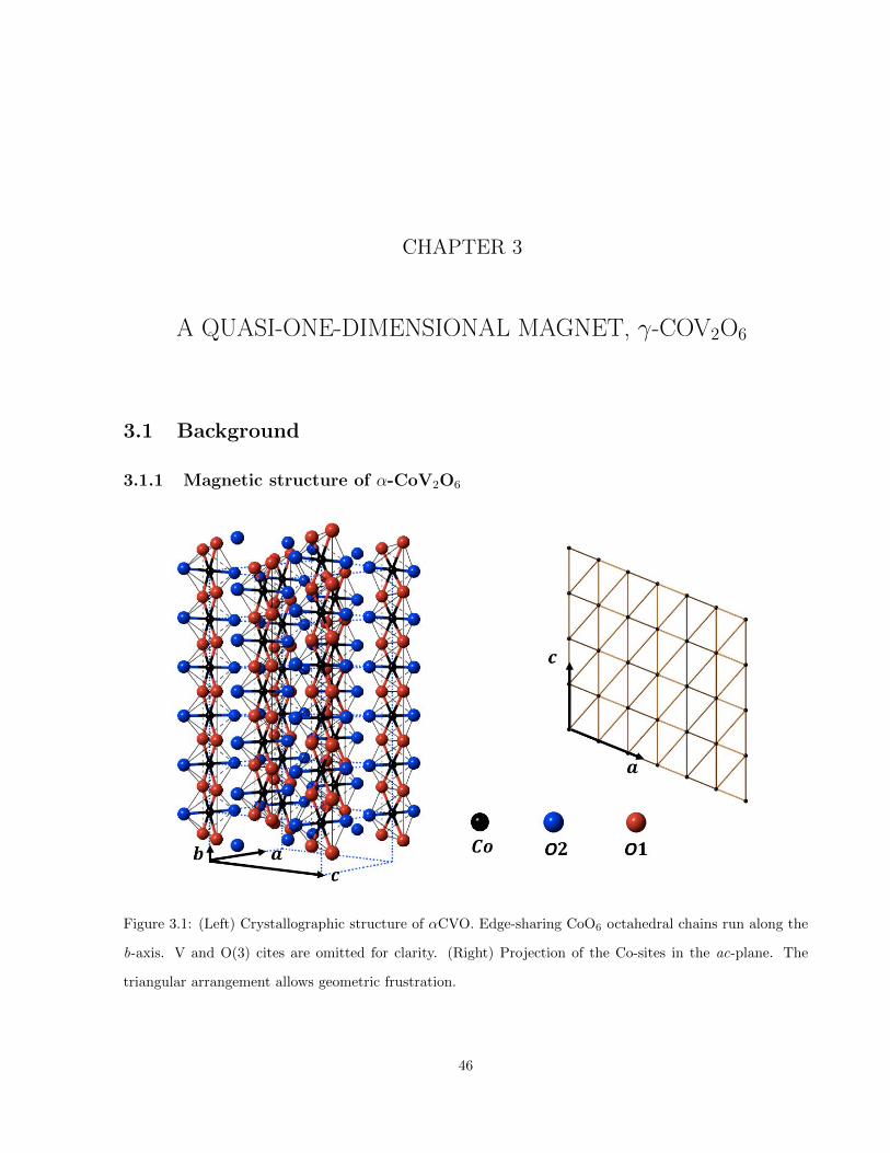
CHAPTER 3
A QUASI-ONE-DIMENSIONAL MAGNET, γ-COV2O6
3.1 Background
3.1.1 Magnetic structure of α-CoV2O6
Figure 3.1: (Left) Crystallographic structure of αCVO. Edge-sharing CoO6 octahedral chains run along the
b-axis. V and O(3) cites are omitted for clarity. (Right) Projection of the Co-sites in the ac-plane. The
triangular arrangement allows geometric frustration.
46

CoV2O6 crystallizes in two polymorphs, the monoclinic α-CoV2O6 (αCVO) and the triclinic γ-CoV2O6
(γCVO) [82, 83]. In both structures, the magnetic Co2+ has 6 nearest neighbour O2−, forming an octahedral
crystal field environment. The space group of αCVO is C2/m. The CoO6 octahedra form edge-sharing
chains along the crystallographic b-axis (Fig. 3.1), which are spatially separated by the VO6 chains. As a
result, the spin lattice of αCVO is quasi-one-dimensional. On the other hand, the space group of γCVO is
P 1. In contrast with the single crystallographic site for Co in αCVO, there are two inequivalent Co sites
in γCVO. Similar to the αCVO case, the γCVO structure also forms edge-sharing CoO6 chains along the
b-axis, whereas these chains are separated by a complex VO4-VO6 network between them (see next section).
In this section, we will discuss the magnetic properties of αCVO, which have been studied comprehensively
by both experiments and theories. The other polymorph γCVO, which is the focus of this chapter, has not
been as studied in the past. We present these studies in the next section.
T = 300 K a = 9.2531(2) A b = 3.5040(1) A c = 6.6201(1) A β= 111.617
Atom x y z Uiso (A2)
Co 0 0 0 0.0090(10)
V 0.3055(19) 0.5 0.3388(26) 0.0090(10)
O(1) 0.1536(2) 0.5 0.1131(3) 0.0110(6)
O(2) 0.4640(2) 0.5 0.2744(4) 0.0110(6)
O(3) 0.1916(2) 0.5 0.5622(4) 0.0110(6)
Table 3.1: Refined lattice parameters, atomic positions and isotropic displacement parameters (Uiso) of
αCVO at 300 K [84].
The refined structural parameters of αCVO at 300 K can be found in Table. 3.1 [84]. Since the Co-O
bonds (∼ 2 A) in the CoO6 octahedron are much shorter than the others (>3.2 A), the nearest neighbour
(NN) intrachain spin exchange is very strong [85]. Moreover, interchain Co-O-Co superexchange paths are
also found in αCVO. By projecting these paths into the ac-plane, the Co exchange network can be treated as a
quasi-triangular lattice which permits the geometric frustration (Fig. 3.1), as discussed in Chapter 1.3 [84, 15].
Previous susceptibility measurements have revealed that αCVO shows strong Ising anisotropy along the c-
axis (Fig. 3.2a) [86]. Since the saturation magnetic moment along the easy c-axis (4.4µB/Co) greatly exceeds
the spin-only value for Co2+ (3.0µB/Co) (Fig. 3.2b), there must be a strong orbital contribution. Local
structure analysis suggests that Co ions reside in a strongly distorted oxygen-octahedral environment [9, 87].
47
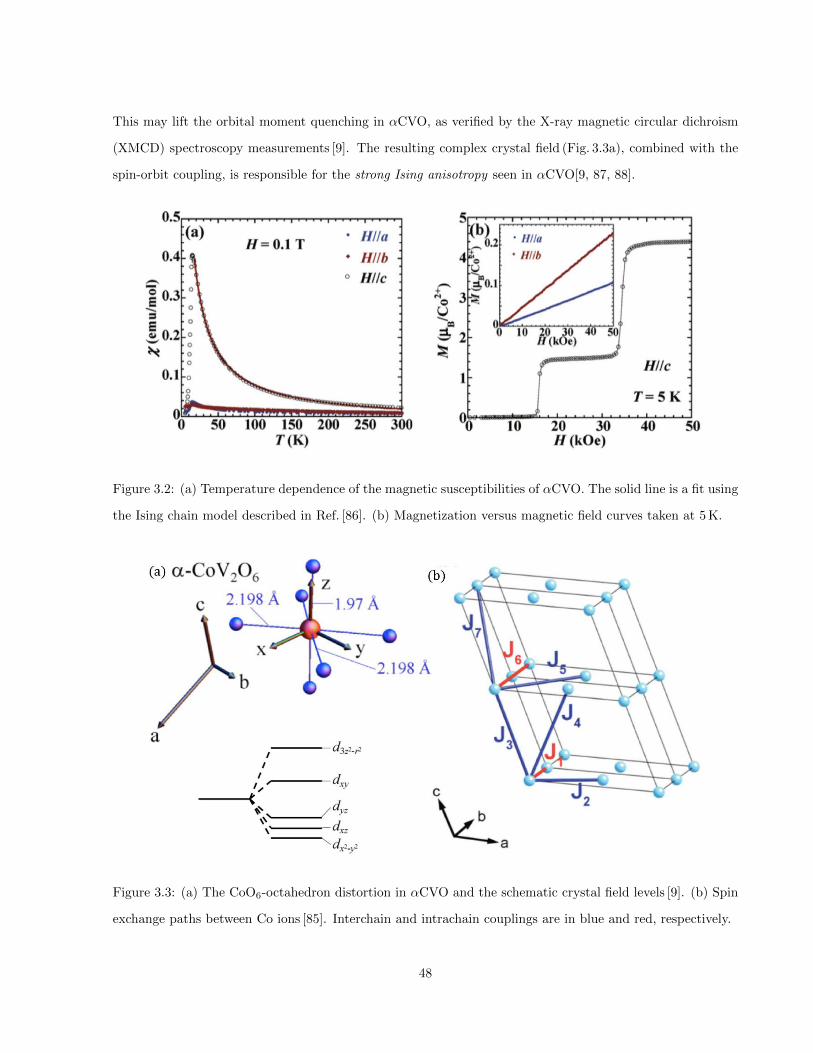
This may lift the orbital moment quenching in αCVO, as verified by the X-ray magnetic circular dichroism
(XMCD) spectroscopy measurements [9]. The resulting complex crystal field (Fig. 3.3a), combined with the
spin-orbit coupling, is responsible for the strong Ising anisotropy seen in αCVO[9, 87, 88].
Figure 3.2: (a) Temperature dependence of the magnetic susceptibilities of αCVO. The solid line is a fit using
the Ising chain model described in Ref. [86]. (b) Magnetization versus magnetic field curves taken at 5 K.
Figure 3.3: (a) The CoO6-octahedron distortion in αCVO and the schematic crystal field levels [9]. (b) Spin
exchange paths between Co ions [85]. Interchain and intrachain couplings are in blue and red, respectively.
48

Besides the strong Ising anisotropy, the competing spin exchange interactions are also crucial to fully
understand the magnetic structure of αCVO (Fig. 3.3b) [85]. For example, a 1/3-plateau in magnetization
can be stablized between 1.6 T and 3.3 T at 5 K by applying a magnetic field along the c-axis (Fig. 3.2b).
This type of metamagnetic transition is a typical manifestation of magnetic frustration [43] and has been
observed in other systems such as Ca3Co2O6 and SrCo6O11 [89, 90]. By taking the longitudinal components
of J1, J2, J3 and J4 (Fig. 3.3b) into an effective Hamiltonian:
H =∑i > j
Jijσiσj − h∑i
σi, (3.1)
where σi is the pseudo-spin variable along the magnetic easy axis at i -site, Saul et al have successfully
reproduced this intermediate 1/3-plateau state (Fig. 3.4a) [85].
Figure 3.4: (a) Simulated magnetization versus magnetic field curve [85]. Inset: the corresponding magnetic
structures in the ac-plane. (b) Magnetic field dependence of lattice parameters (p =a, b, c,β and Volume) [91].
Neutron powder diffraction measurements have also been performed to investigate the magnetic structure
of αCVO [84, 92, 91]. The results are consistent with the theoretical predictions in Ref. [85] (Fig. 3.4a) as
well as the bulk susceptibility data [86, 92]. For the zero field magnetic structure, ferromagnetic Co-chains
along the b-axis are antiferromagnetically coupled to their NN chains in the ac-plane. The spins form a
collinear arrangement in the ac-plane with a tiny tilting angle ∼ 9.3 with respect to the c-axis [92]. For
the 1/3-plateau state, the intrachain spin arrangement is still ferromagnetic. However, there are two spin-up
chains for every one spin-down chain in the ac-plane (Fig. 3.4a). Alternatively, it can be viewed as an ’up-
up-down’ pattern in the ac-plane. At the highest field, where the full saturation is reached, all the interchain
49

spin arrangements become ferromagnetic. In all investigations, the spin orientations have been found to be
insensitive to the magnetic field [84, 92, 91]. In addition, a magnetostructural coupling effect is also observed
in αCVO [84, 92]. The unit cell volume (V) and b-axis are considerably increased between 0 T and 2.5 T
when the antiferromagnetic order is suppressed, as depicted in Fig. 3.4b.
To conclude this part, we now write down a more accurate Hamiltonian to describe the interactions in
αCVO [85]
H = H0 −D∑i
S2iz +
∑i>j
J‖ijSizSjz +
∑i>j
J⊥ij (SixSjx + SiySjy), (3.2)
where H 0 is the spin independent term, D is the single-ion anisotropy constant, x, y, z are the axes in a
Cartesian coordinate system and z is the magnetic easy axis. αCVO can be viewed as a magnet with
strong anisotropy and competing spin interactions. At the limit of D ‖ ~Jij |, it is clear that a collinear
spin structure is favored since having every spin lying along the z -axis will produce the lowest energy [93,
94, 95]. Oppositely, a noncollinear spin structure may be formed if the competing spin exchange terms ( ~Jij)
dominate [93, 94, 95, 96]. It is worth noting that the 1/3-plateau in magnetization can still occur in the
absence of any single-ion anisotropy or geometric frustration [96]. From this point of view, the collinear spin
structure of αCVO is strongly related to the overwhelming single-ion anisotropy in this structure [9, 87].
50
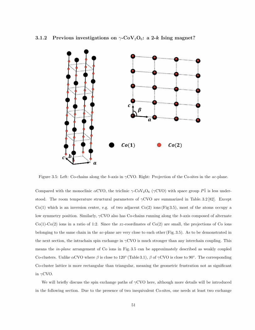
3.1.2 Previous investigations on γ-CoV2O6: a 2-k Ising magnet?
Figure 3.5: Left: Co-chains along the b-axis in γCVO. Right: Projection of the Co-sites in the ac-plane.
Compared with the monoclinic αCVO, the triclinic γ-CoV2O6 (γCVO) with space group P 1 is less under-
stood. The room temperature structural parameters of γCVO are summarized in Table. 3.2 [82]. Except
Co(1) which is an inversion center, e.g. of two adjacent Co(2) ions (Fig 3.5), most of the atoms occupy a
low symmetry position. Similarly, γCVO also has Co-chains running along the b-axis composed of alternate
Co(1)-Co(2) ions in a ratio of 1:2. Since the xz -coordinates of Co(2) are small, the projections of Co ions
belonging to the same chain in the ac-plane are very close to each other (Fig. 3.5). As to be demonstrated in
the next section, the intrachain spin exchange in γCVO is much stronger than any interchain coupling. This
means the in-plane arrangement of Co ions in Fig. 3.5 can be approximately described as weakly coupled
Co-clusters. Unlike αCVO where β is close to 120 (Table 3.1), β of γCVO is close to 90. The corresponding
Co-cluster lattice is more rectangular than triangular, meaning the geometric frustration not as significant
in γCVO.
We will briefly discuss the spin exchange paths of γCVO here, although more details will be introduced
in the following section. Due to the presence of two inequivalent Co-sites, one needs at least two exchange
51
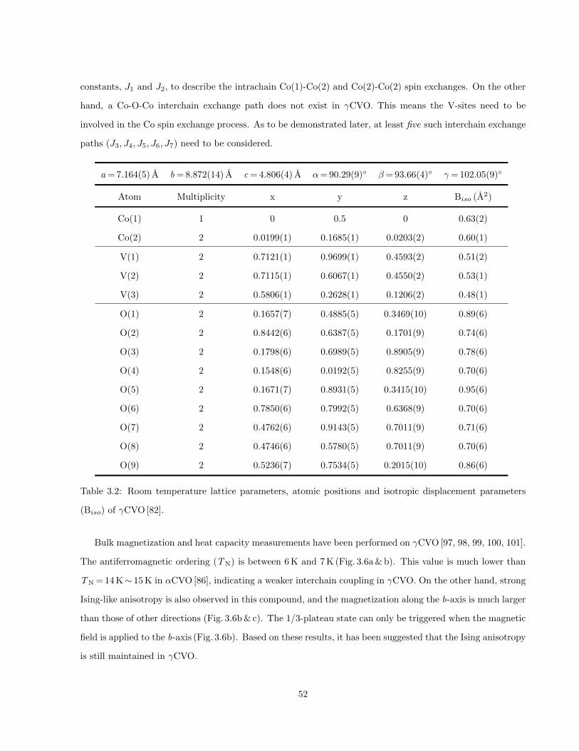
constants, J1 and J2, to describe the intrachain Co(1)-Co(2) and Co(2)-Co(2) spin exchanges. On the other
hand, a Co-O-Co interchain exchange path does not exist in γCVO. This means the V-sites need to be
involved in the Co spin exchange process. As to be demonstrated later, at least five such interchain exchange
paths (J3, J4, J5, J6, J7) need to be considered.
a = 7.164(5) A b = 8.872(14) A c = 4.806(4) A α= 90.29(9) β= 93.66(4) γ= 102.05(9)
Atom Multiplicity x y z Biso (A2)
Co(1) 1 0 0.5 0 0.63(2)
Co(2) 2 0.0199(1) 0.1685(1) 0.0203(2) 0.60(1)
V(1) 2 0.7121(1) 0.9699(1) 0.4593(2) 0.51(2)
V(2) 2 0.7115(1) 0.6067(1) 0.4550(2) 0.53(1)
V(3) 2 0.5806(1) 0.2628(1) 0.1206(2) 0.48(1)
O(1) 2 0.1657(7) 0.4885(5) 0.3469(10) 0.89(6)
O(2) 2 0.8442(6) 0.6387(5) 0.1701(9) 0.74(6)
O(3) 2 0.1798(6) 0.6989(5) 0.8905(9) 0.78(6)
O(4) 2 0.1548(6) 0.0192(5) 0.8255(9) 0.70(6)
O(5) 2 0.1671(7) 0.8931(5) 0.3415(10) 0.95(6)
O(6) 2 0.7850(6) 0.7992(5) 0.6368(9) 0.70(6)
O(7) 2 0.4762(6) 0.9143(5) 0.7011(9) 0.71(6)
O(8) 2 0.4746(6) 0.5780(5) 0.7011(9) 0.70(6)
O(9) 2 0.5236(7) 0.7534(5) 0.2015(10) 0.86(6)
Table 3.2: Room temperature lattice parameters, atomic positions and isotropic displacement parameters
(Biso) of γCVO [82].
Bulk magnetization and heat capacity measurements have been performed on γCVO [97, 98, 99, 100, 101].
The antiferromagnetic ordering (TN) is between 6 K and 7 K (Fig. 3.6a & b). This value is much lower than
TN = 14 K∼ 15 K in αCVO [86], indicating a weaker interchain coupling in γCVO. On the other hand, strong
Ising-like anisotropy is also observed in this compound, and the magnetization along the b-axis is much larger
than those of other directions (Fig. 3.6b & c). The 1/3-plateau state can only be triggered when the magnetic
field is applied to the b-axis (Fig. 3.6b). Based on these results, it has been suggested that the Ising anisotropy
is still maintained in γCVO.
52

Figure 3.6: (a) Heat capacity data of αCVO and γCVO [101]. (b) and (c) Magnetization curves of γCVO
single-crystal and powder [99]. The (b) magnetic field, and (c) temperature scans were taken at T = 1.8 K
and B = 0.1 T, respectively.
Although neutron diffraction has been used to investigate γCVO, the corresponding magnetic structure
has not been fully established to date [98, 99, 100]. Kimber et al observed the magnetic reflections at low
temperatures and could not assign all of the reflections with one propagation vector [98]. However, they
were only able to partially solve the spin structure using a propagation vector k1 = (0.5, 0, 0) (Fig. 3.7a).
The second propagation vector k2, as they pointed out, is perhaps related to the competition between
superexchange interactions and single-ion anisotropy in γCVO (eq. 3.2) [98]. A later investigation carried out
by Lenertz et al confirms k1= (0.5, 0, 0) and proposes k2= (0.25, 0.5, 0) [99]. As shown in Fig. 3.7c, the full
diffraction pattern can be refined using these two modulations. However, they have applied a large number
of hypothetical constraints in the refinement procedure. Most importantly, the peak profile around 2θ= 26
in Fig. 3.7a cannot be fully fitted by the crystallographic structure refinement in Ref. [98], indicating that it
has a magnetic component. Unfortunately, both k1= (0.5, 0, 0) or k2= (0.25, 0.5, 0) fail to produce a magnetic
reflection at this position (corresponding to 2θ= 23∼ 24 in Fig. 3.7c measured by Lenertz et al). As a
result, the complex magnetic structure in γCVO remains to be unveiled.
53

Figure 3.7: Neutron powder diffraction patterns collected by Kimber et al [98] at (a) λ= 2.8 A, T = 2 K and
(b) λ= 1.79 A, T = 2 K and Lenertz et al [99] at (c) λ= 2.423 A, T = 1.7 K.
Compared with αCVO, the CoO6-octahedra in γCVO is much less distorted. This can be characterized
by the following distortion parameter
δ =1
N
∑i
(di− < d >
< d >)2 × 10⁴, (3.3)
where di are the Co-O bond lengths, N = 6 for an octahedron and <d> is the average bond length [87].
It gives δ= 55 in αCVO and δ= 2.1, 4.8 for the two inequivalent Co-sites in γCVO [87]. Correspondingly,
the crystal field splitting should be weak and therefore the orbital quenching stronger in γCVO (Fig. 3.8a),
as confirmed in both experimental and theoretical investigations [88, 99, 9, 97, 100]. This also means the
single-ion anisotropy in this compound is weaker compared with the αCVO case. As discussed in eq. 3.2, a
noncollinear structure is favored when the exchange frustration is dominant in the system. A recent time-of-
flight inelastic neutron spectroscopy study on the powder sample suggests that one-dimensional magnetism
is not able to fully justify their observations [87].
54

To finish this part, we summarize the important points based on previous investigations:
1), γCVO cannot be treated as a geometrically frustrated magnet.
2), Exchange frustration coexists with single-ion anisotropy, whereas the latter is weaker compared with the
αCVO case.
3), Bulk magnetization measurements tend to support the Ising anisotropy and orbital quenching in γCVO.
4), The Ising anisotropy cannot fully account for the inelastic neutron spectroscopy results.
5), Preliminary neutron diffraction measurements indicate a 2-k magnetic structure.
6), The field-induced 1/3-plateau ferrimagnetic (FI) state does not exist in the entire region below TN (3.8b).
Figure 3.8: (a) Local CoO6 enviroments of γCVO and the schematic crystal field level splitting [9]. Magnetic
phase diagram of (b) αCVO and (c) γCVO [101].
55
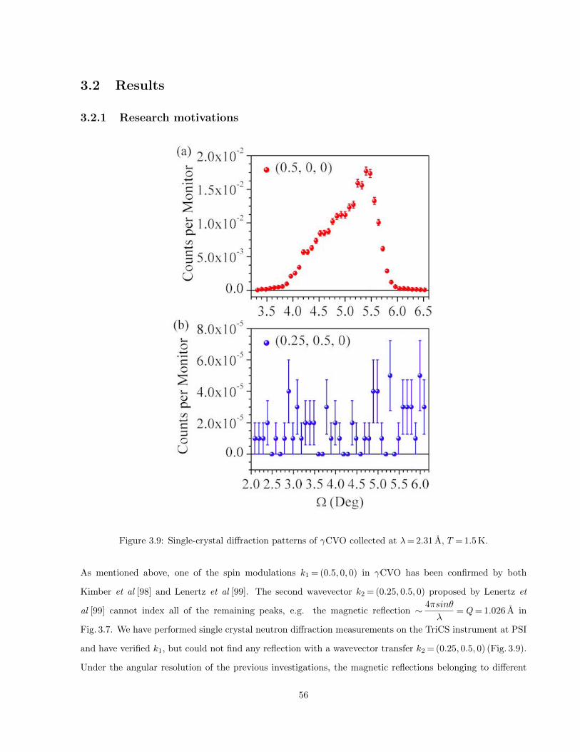
3.2 Results
3.2.1 Research motivations
Figure 3.9: Single-crystal diffraction patterns of γCVO collected at λ= 2.31 A, T = 1.5 K.
As mentioned above, one of the spin modulations k1 = (0.5, 0, 0) in γCVO has been confirmed by both
Kimber et al [98] and Lenertz et al [99]. The second wavevector k2 = (0.25, 0.5, 0) proposed by Lenertz et
al [99] cannot index all of the remaining peaks, e.g. the magnetic reflection ∼ 4πsinθ
λ= Q = 1.026 A in
Fig. 3.7. We have performed single crystal neutron diffraction measurements on the TriCS instrument at PSI
and have verified k1, but could not find any reflection with a wavevector transfer k2 = (0.25, 0.5, 0) (Fig. 3.9).
Under the angular resolution of the previous investigations, the magnetic reflections belonging to different
56
modulations are highly overlapped. For example, there are only 3 visible reflections not indexed by k1 in
Fig. 3.7a, which makes it very hard to exactly determine k2. Moreover, the Ising anisotropy revealed by the
bulk magnetization measurements does not coincide with the inelastic neutron scattering data carried out
by Wallington et al [87]. Apparently, the magnetic structure of γCVO is the key to answer this question. As
a result, further neutron diffraction investigations on γCVO with a better resolution are highly demanded.
We therefore carried out a new neutron powder diffraction study.
3.2.2 Data collection and analysis
Both single crystals and powders of γCVO were investigated. Powder samples have were synthesized using
the ceramic method. A homogeneous mixture of CoC2O4 ·H2O and V2O5 in a molar ratio of 1 : 1 were
sintered at 873 K in air for 80 hours. The single crystals of γCVO were grown by the flux method; details of
the procedure are given in Ref. [97]. Magnetic susceptibility data were collected using a Magnetic Property
Measurement System (MPMS, Quantum Design). The existence of magnetic frustration in γCVO is exper-
imentally supported by the commonly used frustration index f = |θCW/TN| = 1.66(3) (θCW: Curie-Weiss
temperature, TN: Neel temperature). We carried out diffraction measurements on powder samples using the
cold neutron powder diffractometer DMC at the Swiss Spallation Neutron Source (SINQ). Two neutron wave-
lengths, 2.4586 A and 4.5 A, were used. The longer wavelength provided the necessary angular resolution to
distinguish the magnetic Bragg peaks. 6 g of powder was loaded into a thin Al cylinder (6 mm in diameter) and
then into a cryostat to probe temperatures down to 1.5 K. Single crystal neutron diffraction measurements
were performed on the TriCS instrument at SINQ. These data (not shown here) confirm the propagation vec-
tor k1 = (0.5, 0, 0) of the magnetic structure found by Kimber et al. [98] and Lenertz et al. [99], but we did not
find peaks corresponding to the second propagation vector (0.25, 0.5, 0) proposed in Ref. [99]. Furthermore,
we find a magnetic Bragg peak at Q' 1.03 A−1 in our powder diffraction profiles (Fig. 3.13) that cannot be
indexed using either of the previously found propagation vectors.
The neutron powder diffraction patterns have been analyzed using the FullProf package [102]. This soft-
ware is based on a least-squares method called ‘Rietveld refinement’ [103]. The basic principles of Rietveld
refinement are discussed in Appendix A. In order to solve the magnetic and crystallographic structure of
γCVO at low temperatures, we have chosen to simultaneously refine two patterns collected under different
wavelengths (4.5 A and 2.4586 A). The shorter wavelength enables us to determine the crystallographic struc-
ture, whereas the longer wavelength offers necessary angular resolution to determine the correct k2 and then
to solve the magnetic structure. Here we have chosen to demonstrate the refinement procedure under the two
57
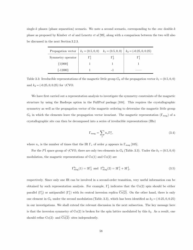
single-k phases (phase separation) scenario. We note a second scenario, corresponding to the one double-k
phase as proposed by Kimber et al and Lenertz et al [99], along with a comparison between the two will also
be discussed in the next Section 3.2.3.
Propagation vector k1 = (0.5, 0, 0) k1 = (0.5, 0, 0) k2 = (-0.25, 0, 0.25)
Symmetry operator Γ11 Γ1
2 Γ11
1|000 1 1 1
-1|000 1 -1 ——
Table 3.3: Irreducible representations of the magnetic little group Gk of the propagation vector k1 = (0.5, 0, 0)
and k2 = (-0.25, 0, 0.25) for γCVO.
We have first carried out a representation analysis to investigate the symmetry constraints of the magnetic
structure by using the BasIreps option in the FullProf package. [104]. This requires the crystallographic
symmetry as well as the propagation vector of the magnetic ordering to determine the magnetic little group
Gk in which the elements leave the propagation vector invariant. The magnetic representation (Γmag) of a
crystallographic site can then be decomposed into a series of irreducible representations (IRs)
Γmag =∑v
nvΓµv , (3.4)
where nv is the number of times that the IR Γv of order µ appears in Γmag [105].
For the P 1 space group of γCVO, there are only two elements in Gk (Table. 3.3). Under the k1 = (0.5, 0, 0)
modulation, the magnetic representations of Co(1) and Co(2) are
Γk1mag(1) = 3Γ1
2 and Γk1mag(2) = 3Γ1
1 + 3Γ12, (3.5)
respectively. Since only one IR can be involved in a second-order transition, very useful information can be
obtained by such representation analysis. For example, Γ12 indicates that the Co(2) spin should be either
parallel (Γ12) or antiparallel (Γ1
1) with its central inversion replica Co(2). On the other hand, there is only
one element in Gk under the second modulation (Table. 3.3), which has been identified as k2 = (-0.25, 0, 0.25)
in our investigations. We shall extend the relevant discussion in the next subsection. The key message here
is that the inversion symmetry of Co(2) is broken for the spin lattice modulated by this k2. As a result, one
should refine Co(2)- and Co(2)- sites independently.
58

Figure 3.10: Powder diffraction patterns obtained at T = 1.5 K. The calculated pattern (black solid lines)
correspond to the first step described in the context. The vertical bars, from top to bottom, label the
reflections of nuclear, k1, k2 and Aluminium (sample holder), respectively. The Rietveld factors (Appendix A)
are also displayed.
59
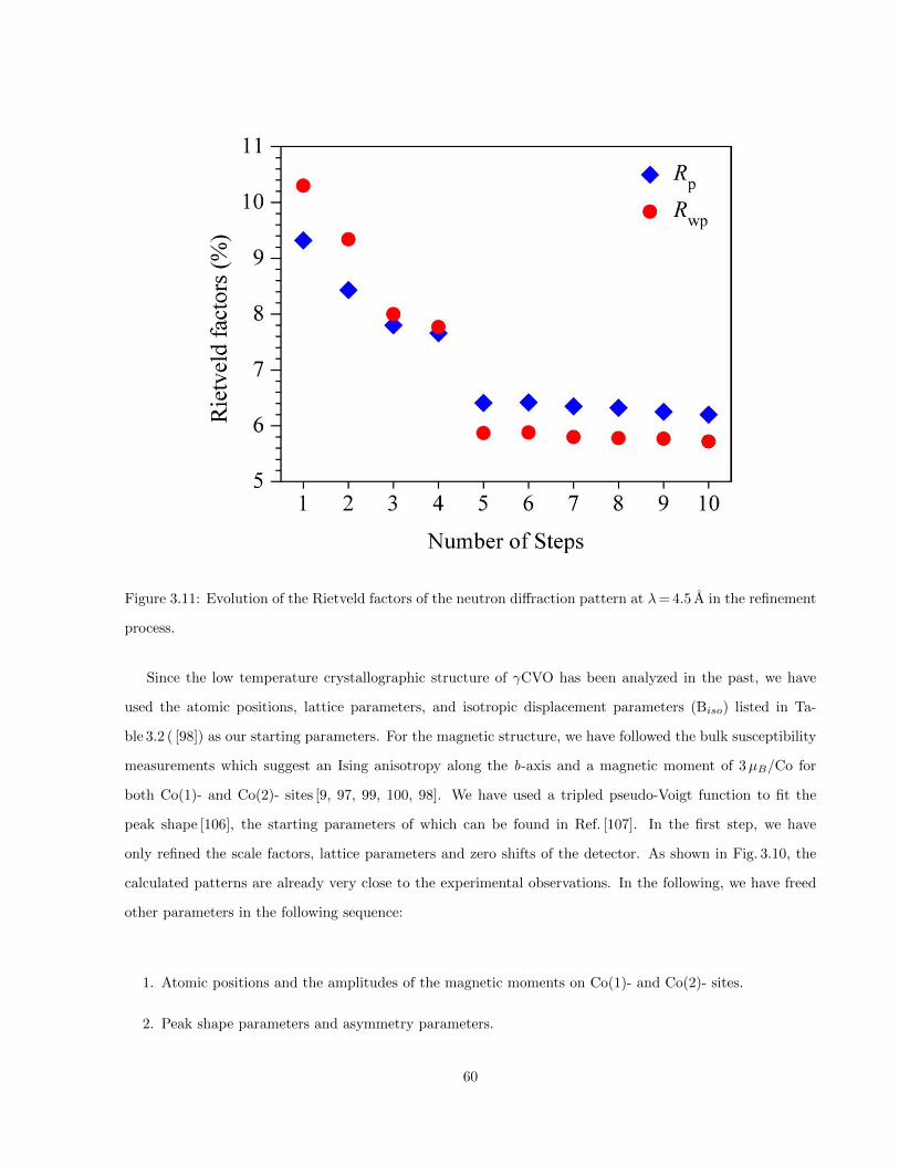
Figure 3.11: Evolution of the Rietveld factors of the neutron diffraction pattern at λ= 4.5 A in the refinement
process.
Since the low temperature crystallographic structure of γCVO has been analyzed in the past, we have
used the atomic positions, lattice parameters, and isotropic displacement parameters (Biso) listed in Ta-
ble 3.2 ( [98]) as our starting parameters. For the magnetic structure, we have followed the bulk susceptibility
measurements which suggest an Ising anisotropy along the b-axis and a magnetic moment of 3µB/Co for
both Co(1)- and Co(2)- sites [9, 97, 99, 100, 98]. We have used a tripled pseudo-Voigt function to fit the
peak shape [106], the starting parameters of which can be found in Ref. [107]. In the first step, we have
only refined the scale factors, lattice parameters and zero shifts of the detector. As shown in Fig. 3.10, the
calculated patterns are already very close to the experimental observations. In the following, we have freed
other parameters in the following sequence:
1. Atomic positions and the amplitudes of the magnetic moments on Co(1)- and Co(2)- sites.
2. Peak shape parameters and asymmetry parameters.
60
3. Background.
4. Spin orientation of Co(1) in the k1 phase.
5. Spin orientation of Co(2) in the k1 phase.
6. Spin orientation of Co(1) in the k2 phase.
7. Spin orientation of Co(2) in the k2 phase.
For the k1 modulation, several initial trials have ruled out Γ12 on Co(2)-sites. This produces a zigzag
ferromagnetic Co chain along the b-axis. For the k2 modulation, several constraints have been applied during
the fitting process. This will be discussed in the next subsection. By ending this subsection, we note that the
refinement converges in each step and the fitting quality is also greatly improved over this process (Fig. 3.11).
3.2.3 Magnetic phase separation in γ-CoV2O6
Magnetic frustration occurs when a system’s total free energy cannot be minimized by optimizing the inter-
action energy between every pair of spins. This can be caused by competing interactions [96] or by geometry
e.g. antiferromagnetic interactions on a triangular or tetrahedral unit [15]. As a result, the ground state of
a frustrated magnet is often highly degenerate [1]. The degeneracy can be lifted by perturbations such as
additional interaction terms [15], quantum fluctuations [108], and so forth. Various exotic spin states may also
result, as found by numerical simulations [109, 110]. Evidently, experiments are essential to verify the nature
of the interactions, determine their parameters and to confirm the presence of any emergent states.
Another consequence of competing interactions may be phase separation, a common phenomenon among
colossal magneto-resistance (CMR) manganites and high-T c superconductors [10, 111]. There are no con-
straints on the type of these interactions, though so far most phase separation phenomena require non-
magnetic Hamiltonian terms (e.g. Coulomb interaction, electron-phonon coupling). Recently, phase separation
possibly of purely magnetic origin was studied in SrCo6O11 where a ‘devil’s staircase’ is realised [112], though
the volume fractions of the competing phases were not determined. Dynamic phase separation has also been
observed in the quasi-one-dimensional (Q1D) Ca3Co2O6 [40] and possible microphases have also been reported
here [43, 42]. To our knowledge, static or dynamic phase separation exclusively caused by competing spin
exchange interactions, e.g. exchange frustration, on a non-geometrically frustrated lattice has not presently
been reported.
61

Figure 3.12: (a) Crystal structure of triclinic γCVO. Oxygen anions (omitted for clarity) occupy the corner
of the shaded polyhedra. (b) Possible interchain spin exchange paths displayed in two unit cells for Co(1)
and Co(2), respectively.
We report magnetic phase separation in the triclinic cobaltate compound γ-CoV2O6 (γCVO). γCVO has
space group P1 with edge-sharing CoO6-octahedra arranged in zigzag chains along the crystallographic b-
axis. These chains are well separated by a VO4-VO6 polyhedral-network between them (Fig. 3.12a) [82]. Unlike
its polymorph α-CoV2O6 (αCVO), the transverse nearest neighbour (NN) exchange in γCVO must involve
V5+ [86]. This significantly weakens the interchain exchange interaction strength as evidenced by a lower
ordering temperature in γCVO [86, 97, 98]. As shown in Fig. 3.12a, there are two inequivalent cobalt sites,
Co(1) and Co(2). For the Co(2)-Co(2) exchange, there is only one Co2+-O2−-V5+-O2−-Co2+ (COVOC)
path along the a-axis (Fig. 3.12b). In contrast, two very similar COVOC paths are found along the c-axis,
affording the possibility of the so-called ‘random frustration’ caused by competing interactions [15]. For the
Co(1)-Co(1) exchange, no NN COVOC path is found along the a-axis and only one such path is located
along the c-axis. Surprisingly, a skew path between interchain Co(1) and Co(2) sites is also found. Its length
is close to those of the transverse ones, meaning these skew paths are just as important for the magnetic
structure. First of all, they can set up correlations between Co(1) spins along the a-axis. Second, since the
62

intrachain exchange is mainly ferromagnetic, an antiferromagnetic skew exchange would complicate the final
magnetic structure or even lead to further frustration.
Figure 3.13: Neutron powder diffraction pattern measured at λ= 4.5 A, T = 1.5 K. The red solid dots are
experimental observations. The black and blue lines are the calculated pattern and the difference using the
2 -phase model. Black, pink and green vertical bars mark the nuclear, k1- and k2- modulated Bragg positions,
respectively. Right inset: Sketch of the ac-plane magnetic structure modulated by k2 in a 5x5 unit cell. Left
inset: A weak reflection indexed as (0.5, 1, 0) around 0.931 A.
On cooling the system down to 1.5 K from the paramagnetic state, magnetic Bragg peaks are observed
in the low-Q region (Fig. 3.13). The refined lattice parameters (Table 3.4) are consistent with previous
works [98, 99]. In addition to the k1 = (0.5, 0, 0) wavevector proposed by Kimber et al. [98], corresponding
to ferromagnetic bc-planes antiferromagnetically coupled along the a-axis, we find that a second propa-
gation vector k2 = (-0.25, 0, 0.25) is required to index the rest of the peaks. The in-plane spin modulation
of k2 is shown schematically in the right inset of Fig. 3.13. We also find short range correlations down to
the lowest temperature probed (1.5 K). Their contributions below the incommensurate-commensurate lock-
in transition T ∗= 5.6 K are treated in two self-consistent ways: (a) Gaussian functions are used to fit the
diffuse profiles on the tails of the main peaks at Q1 = (−0.25, 0, 0.25) at ∼ 0.39 A−1 and Q2 = (0.5, 0, 0)
63
at ∼ 0.45 A−1, respectively (Fig. 3.15b). The background is fixed during the refinement after subtraction of
such profiles. (b) Alternatively, they are regarded as a part of the background so that the background is also
refined. These two methods produce essentially identical magnetic structures within our fitting resolution.
Although rare, multi-k structures have been predicted and experimentally confirmed in some frustrated
systems [113, 114, 109, 110, 115, 116]. We therefore propose two possible magnetic structures for γCVO: (I) a
single phase with 2-k-modulation, or (II) two 1-k phases (phase separation). As shown by the Rietveld factors
in Table 3.4, both scenarios turn out to fit the data reasonably well, although with some caveats. Possible
phase differences between the two inequivalent Co-sites and between the two modulations have been fixed
to zero, since we found that these parameters either resulted in unphysically large magnetic moments or did
not converge within the fitting resolution. We could not solve exactly the spin orientations modulated by k2
in either scenario, since the relevant free parameters were highly correlated, resulting in unphysically large
standard deviations in the Rietveld refinements.
We have also tested a ‘minimal model’ for each scenario where all spins modulated by k2 lie along the b-
direction; this is based on the assumption of Ising-like anisotropy along the crystallographic b-axis [97, 99, 100].
This minimal model was then relaxed by allowing spin canting in the ab-, or bc- plane on each Co-site. For
the 2-k single phase scenario, this canting does not improve the original refinement produced by the minimal
model, and so the corresponding spin orientations are fixed to the b-axis. In a triclinic lattice, we note the spins
will still have components in the ac-plane even if the b-axis Ising anisotropy is strictly followed (Table 3.4).
The refinement is not sensitive to additional spin canting on Co(1)-sites in the phase separation scenario
(fixed along the b-axis for these sites in Table 3.4), but it is considerably improved by including canting in
the bc-plane on Co(2)-sites (see below).
Both scenario I and II fit the data reasonably well. However, the global average of the magnetic moment
along the b-axis (M b) obtained by the 2-k solution is 4.3(3) µB . This is close to the value in αCVO where
there is large spin-orbit coupling (SOC) [86, 92, 84, 9]. Crystallographic structure analysis shows that the
distortion of the CoO6-octahedron is much weaker in γCVO than in αCVO [87]. This leads to a very small
orbital contribution to the total moment in γCVO, as revealed by X-ray magnetic circular dichroism (XMCD)
spectroscopy and theoretical calculations [9, 88]. The result is a global average spin moment of ∼ 3.2µB/Co,
mainly pointing along the b-axis, in agreement with magnetization measurements [98, 100, 99, 97]. We
point out that the 2-~k solution is inconsistent with this value. On the other hand, the phase separation
model produces M b = 3.04(9) µB/Co, in excellent agreement with magnetization, XMCD data, as well as
theoretical predictions [9, 88, 98, 100, 99, 97].
64

Scenario I 2-k
a, b, c (A) 7.1515(4) 8.8555(3) 4.7951(2)
α,β, γ () 90.144(5) 93.948(2) 102.110(6)
Moments Ma (µB) Mb (µB) Mc (µB)
Co(1) : k1 -0.5(2) 2.5(1) 0.3(3)
Co(2) : k1 0.2(1) 2.44(7) -0.5(2)
Co(2) : k1 0.2(1) 2.44(7) -0.5(2)
Co(1) : k2 -0.4(1) 2.0(6) -0.01(1)
Co(2) : k2 -0.21(4) 1.0(2) -0.003(4)
Co(2) : k2 -0.5(1) 2.5(5) -0.01(1)
Scenario II† 2-phase
a, b, c (A) 7.1524(4) 8.8560(3) 4.7954(2)
α,β, γ () 90.137(6) 93.949(2) 102.122(7)
Moments Ma (µB) Mb (µB) Mc (µB)
Co(1) : k1 [65(1) %] -1.7(3) 2.9(3) 1.1(3)
Co(2) : k1[65(1) %] -1.1(2) 3.1(1) -0.2(2)
Co(2) : k1[65(1) %] -1.1(2) 3.1(1) -0.2(2)
Co(1) : k2[35(1) %] -0.69(4) 3.3(2) 0.008(4)
Co(2) : k2[35(1) %] -0.57(5) 2.8(2) 1.5(4)
Co(2) : k2[35(1) %] -0.65(2) 3.1(1) -0.008(2)
Rietveld factors Rp (%) Rwp(%) χ2
2-k 6.29 5.78 4.796
2-phase• 6.25 5.77 4.749
2-phase† 6.20 5.72 4.657
2-phase‡ 6.20 5.77 4.728
Table 3.4: Magnetic and lattice parameters of γCVO at T = 1.5 K. Constraints on the spin orientations for
the k2 modulation have been applied; see main text for details. Co(2) is the central inversion replica of Co(2).
The isotropic displacement parameters (Biso) and V atomic positions were fixed to the values reported in
Ref. [98]. Lattice parameters, O and Co positions were refined using data at λ = 2.4586 A. Three sets of
Rietveld factors, corresponding to the minimal model (•), inequivalent (†) and equivalent (‡) spin canting on
Co(2)- and Co(2)- sites, are listed for the 2-phase scenario.
65
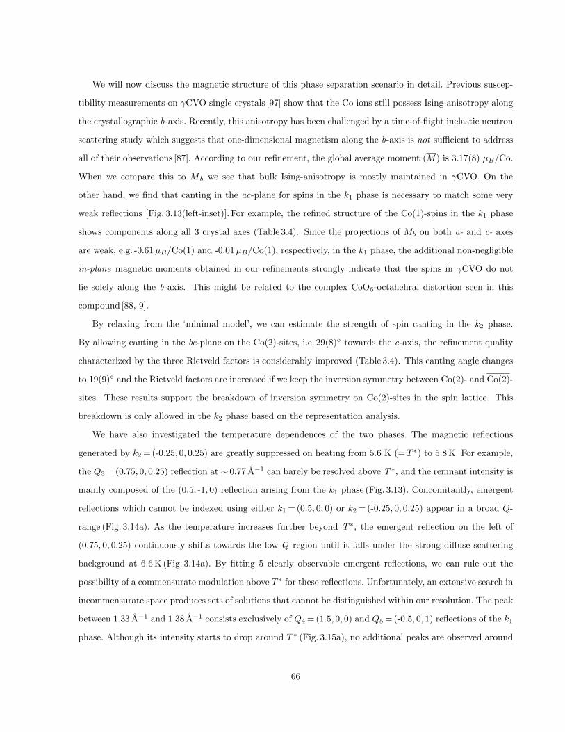
We will now discuss the magnetic structure of this phase separation scenario in detail. Previous suscep-
tibility measurements on γCVO single crystals [97] show that the Co ions still possess Ising-anisotropy along
the crystallographic b-axis. Recently, this anisotropy has been challenged by a time-of-flight inelastic neutron
scattering study which suggests that one-dimensional magnetism along the b-axis is not sufficient to address
all of their observations [87]. According to our refinement, the global average moment (M) is 3.17(8) µB/Co.
When we compare this to M b we see that bulk Ising-anisotropy is mostly maintained in γCVO. On the
other hand, we find that canting in the ac-plane for spins in the k1 phase is necessary to match some very
weak reflections [Fig. 3.13(left-inset)]. For example, the refined structure of the Co(1)-spins in the k1 phase
shows components along all 3 crystal axes (Table 3.4). Since the projections of Mb on both a- and c- axes
are weak, e.g. -0.61µB/Co(1) and -0.01µB/Co(1), respectively, in the k1 phase, the additional non-negligible
in-plane magnetic moments obtained in our refinements strongly indicate that the spins in γCVO do not
lie solely along the b-axis. This might be related to the complex CoO6-octahehral distortion seen in this
compound [88, 9].
By relaxing from the ‘minimal model’, we can estimate the strength of spin canting in the k2 phase.
By allowing canting in the bc-plane on the Co(2)-sites, i.e. 29(8) towards the c-axis, the refinement quality
characterized by the three Rietveld factors is considerably improved (Table 3.4). This canting angle changes
to 19(9) and the Rietveld factors are increased if we keep the inversion symmetry between Co(2)- and Co(2)-
sites. These results support the breakdown of inversion symmetry on Co(2)-sites in the spin lattice. This
breakdown is only allowed in the k2 phase based on the representation analysis.
We have also investigated the temperature dependences of the two phases. The magnetic reflections
generated by k2 = (-0.25, 0, 0.25) are greatly suppressed on heating from 5.6 K (=T ∗) to 5.8 K. For example,
the Q3 = (0.75, 0, 0.25) reflection at ∼ 0.77 A−1 can barely be resolved above T ∗, and the remnant intensity is
mainly composed of the (0.5, -1, 0) reflection arising from the k1 phase (Fig. 3.13). Concomitantly, emergent
reflections which cannot be indexed using either k1 = (0.5, 0, 0) or k2 = (-0.25, 0, 0.25) appear in a broad Q-
range (Fig. 3.14a). As the temperature increases further beyond T ∗, the emergent reflection on the left of
(0.75, 0, 0.25) continuously shifts towards the low-Q region until it falls under the strong diffuse scattering
background at 6.6 K (Fig. 3.14a). By fitting 5 clearly observable emergent reflections, we can rule out the
possibility of a commensurate modulation above T ∗ for these reflections. Unfortunately, an extensive search in
incommensurate space produces sets of solutions that cannot be distinguished within our resolution. The peak
between 1.33 A−1 and 1.38 A−1 consists exclusively of Q4 = (1.5, 0, 0) and Q5 = (-0.5, 0, 1) reflections of the k1
phase. Although its intensity starts to drop around T ∗ (Fig. 3.15a), no additional peaks are observed around
66

Figure 3.14: (a) Selected regions of the powder diffraction patterns between 5.4 K and 6.6 K, showing theshifting reflections. The peak positions in the intermediate region are fitted with Gaussian functions (solidlines). A constant vertical shift has been applied to patterns measured above T ∗. The remnant peak aboveT ∗ is indexed as (0.5, -1, 0). (b) Temperature dependence of the (1.5, 0, 0) and (-0.5, 0, 1) reflections generatedby k1, which in contrast do not shift. (c) Temperature dependences of the x and z components of k2 aroundT ∗.
67

it (Fig. 3.14b). This suggests that the appearance of the incommensurate peaks above T ∗ is not related to the
k1 phase. Since previous heat capacity measurements did not reveal any phase transition at T ∗ [97, 98, 101],
these features are consistent with a commensurate-incommensurate lock-in transition of the k2 phase. We find
that only two of the three components of the general incommensurate wavevector, k2 = (kx, ky, kz), can be
uniquely determined at each temperature from the 5 clearly observable incommensurate peaks. Setting ky = 0,
we may plot the temperature dependence of k2 = (kx, 0, kz) in Fig. 3.14c. The temperature dependence of the
normalized integrated intensity of the Q3 reflection is also plotted in Fig. 3.15a. TN for the k1 phase has been
determined to be 6.6 K (the corresponding normalized intensity versus temperature plot has the steepest slope
at this point). Since no reflection indexed by k2 can be observed above TN, we expect that both phases share
the same transition temperature. It is also worth noting that both solutions only give one reflection between
0.6 A−1 and 0.74 A−1. Correspondingly, the Q3 reflection is not resolution limited (Fig. 3.14a), meaning that
the k2 phase becomes short range ordered between T ∗ and TN.
Strong diffuse scattering profiles appear above T ∗ (Fig. 3.15c), and are detectable up to 25 K (Fig. 3.15d).
When T >TN, the magnetic incoherent scattering background is stabilized, making it possible to study the
pure magnetic diffuse scattering signals by subtracting the nuclear contributions taken at 35 K. As shown in
Fig. 3.15b, these profiles still center around Q1 at TN. Fitting them with a Lorentzian function produces a
correlation length (ξ) of 94(4) A. This is much smaller than ξ∼ 230 A at 1.5 K by fitting the diffuse tails of
Q1 and Q2 reflections (Fig. 3.15b). Although spin fluctuations set in well above TN in γCVO, it is very hard
to extract their positions at high temperatures due to the extra scattering signals from small angles as well
as the weak intensities. However, these spin fluctuations are more related to the k2 modulation, as revealed
by our analysis at temperatures close to TN. Given that the k1 phase populates the majority (∼ 65 %) of the
sample, the dominant spin fluctuations related to k2 above TN are very surprising.
Incommensurate magnetic microphases with a metastable propagation vector have been studied theoreti-
cally on a geometrically frustrated lattice with Ising anisotropy [43]. At very low temperatures, the magnetic
structure is commensurate, while metastable incommensurate microphases exist in the intermediate region. It
is also suggested that additional subtle coupling terms may stabilize the incommensurate state, as realized
in Ca3Co2O6 [39]. On the other hand, both single-ion anisotropy and exchange frustration are present in
both αCVO and γCVO [87, 88]. As suggested in Refs. [93, 94, 95, 96], the system will form a collinear spin
structure if the single-ion anisotropy is stronger compared with the spin exchange interactions, whereas an
incommensurate noncollinear spin structure is favoured oppositely. The collinear spin arrangement of αCVO,
which possesses a very strong SOC, is consistent with this description [84, 92, 9, 87]. For the γCVO compound
68
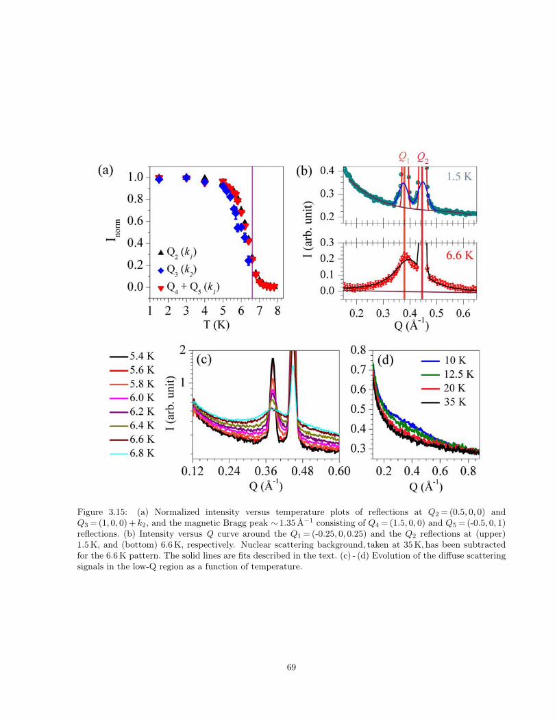
Figure 3.15: (a) Normalized intensity versus temperature plots of reflections at Q2 = (0.5, 0, 0) andQ3 = (1, 0, 0) + k2, and the magnetic Bragg peak ∼ 1.35 A−1 consisting of Q4 = (1.5, 0, 0) and Q5 = (-0.5, 0, 1)reflections. (b) Intensity versus Q curve around the Q1 = (-0.25, 0, 0.25) and the Q2 reflections at (upper)1.5 K, and (bottom) 6.6 K, respectively. Nuclear scattering background, taken at 35 K, has been subtractedfor the 6.6 K pattern. The solid lines are fits described in the text. (c) - (d) Evolution of the diffuse scatteringsignals in the low-Q region as a function of temperature.
69
where the SOC is much weaker [9], we propose it is close to the collinear-noncollinear phase boundary. The 2 -
phase separation may be caused by local chemical disorder. Alternatively, other types of interactions may be
required to further stablize such a state. For example, it has been suggested that the magnetoelectric coupling
is responsible for the additional ferrimagnetic microphase in Ca3Co2O6 [42]. We note this term is also allowed
for the k2 phase of γCVO due to the broken inversion symmetry of the Co(2) spin lattice [117, 118, 119].
Finally, the complexity of magnetism in γCVO can be further stressed by the reported observation on single
crystal samples of magnetic reflections possibly indexed by k3 = (-1/3, 0, 1/3) below T ∗ [100], which are not
seen in our study.
70
3.3 Conclusions and future work
In summary, we have investigated the magnetism of γCVO as a function of temperature using neutron
powder diffraction technique. We have established that its low temperature spin structure essentially consists
of two single-k phases in a ratio about 65(1) : 35(1). This is the first confirmation of phase separation in
a material possessing magnetic ‘exchange frustration’ but not ‘geometric frustration’. For the minority
phase, a crossover between long range commensurate and short range incommensurate magnetic order is
observed at T ∗. Above the magnetic ordering temperature, strong spin fluctuations are observed. Within
our experimental resolution, these fluctuations are exclusively modulated k2.
γCVO can be described by the Hamiltonian writen in Eq. 3.2. Compared with αCVO, the single-ion
anisotropy term is weaker in γCVO. This may be responsible for the noncollinear spin structure of the k2
phase. The onset of the collinear k1 phase may indicate the anisotropy constant (D) and spin exchange
constants (J⊥, J‖) are lying in the critical region where k1 and k2 states are degenerate. Alternatively, phase
separation indicates Eq. 3.2 may be inadequate to describe γCVO.
Further investigations on this compound are demanded. From a theoretical point of view, it is essential
to establish a model which can produce phase separation and incommensurate-commensurate crossover in
one of the phases. On the other hand, we shall also perform diffraction measurements on single-crystals
to exactly solve its magnetic structure. As discussed in Ref. [118, 117], a magnetoelectric coupling effect is
possible in similar systems. Moreover, the polarized neutron diffraction technique is a powerful tool to study
the nature of the short range correlation at high temperatures.
71

CHAPTER 4
MIXED-VALENCE MANGANESE PEROVSKITE,
PR0.5CA0.5MN0.97GA0.03O3
4.1 Background
4.1.1 Multiple scale phase separation and colossal magnetoresistance
Colossal magnetoresistance (CMR), which describes a drastic drop in resistance caused by either magnetic
field or temperature (Fig. 4.1b), is commonly observed in mixed-valence manganites [2, 10]. Spatial inhomo-
geneities can spontaneously develop in these materials (phase separation, see Chapter 1.4.2). Phase separa-
tion on atomic scales, including polarons (Fig. 4.1c), charge order, orbital order, is often referred as electronic
phase separation. This can be related to electron-lattice coupling, electron-electron Coulomb repulsion, and
so forth [2, 10]. On the other hand, phase separation on a scale of several hundred nanometres to a few
micrometres (Fig. 4.1c) is typically caused by disorder or strains [2, 10, 54].
Currently, it is widely believed that CMR is triggered by the collapse of phase separation on multiple
scales [2, 10, 46, 47]. As illustrated in Fig. 4.1, micrometre-scale ferromagnetic metallic domains, which
percolate while a large enough magnetic field is applied, have been observed in La1−xCaxMnO3 (x∼ 0.3) [61].
Correspondingly, CMR in this compound has also been found to correlate with the collapse of polarons
(Fig. 4.1c) [120, 56, 57]. These results suggest that both types of phase separation are important to the
carrier transport in La1−xCaxMnO3 (x∼ 0.3). However, the specific role of each phase in the magnetoresistive
process is not clear to date. For example, carrier delocalization is often linked to the ferromagnetic Zener
double-exchange (DE) [10, 60, 61, 58, 121, 57, 122]. At first sight, this statement may be correct since the
ferromagnetic order favors a metal-like state [2]. However, it is questionable in CMR manganites, where the
driving mechanism of carrier localization is not DE [2, 10, 46]. Especially for systems showing atomic scale
72
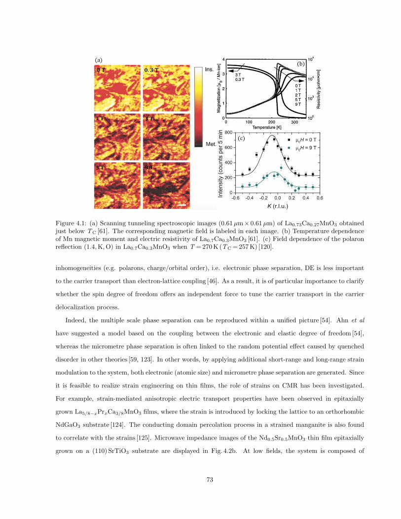
Figure 4.1: (a) Scanning tunneling spectroscopic images (0.61µm× 0.61µm) of La0.73Ca0.27MnO3 obtainedjust below TC [61]. The corresponding magnetic field is labeled in each image. (b) Temperature dependenceof Mn magnetic moment and electric resistivity of La0.7Ca0.3MnO3 [61]. (c) Field dependence of the polaronreflection (1.4, K, O) in La0.7Ca0.3MnO3 when T = 270 K (TC = 257 K) [120].
inhomogeneities (e.g. polarons, charge/orbital order), i.e. electronic phase separation, DE is less important
to the carrier transport than electron-lattice coupling [46]. As a result, it is of particular importance to clarify
whether the spin degree of freedom offers an independent force to tune the carrier transport in the carrier
delocalization process.
Indeed, the multiple scale phase separation can be reproduced within a unified picture [54]. Ahn et al
have suggested a model based on the coupling between the electronic and elastic degree of freedom [54],
whereas the micrometre phase separation is often linked to the random potential effect caused by quenched
disorder in other theories [59, 123]. In other words, by applying additional short-range and long-range strain
modulation to the system, both electronic (atomic size) and micrometre phase separation are generated. Since
it is feasible to realize strain engineering on thin films, the role of strains on CMR has been investigated.
For example, strain-mediated anisotropic electric transport properties have been observed in epitaxially
grown La5/8−xPrxCa3/8MnO3 films, where the strain is introduced by locking the lattice to an orthorhombic
NdGaO3 substrate [124]. The conducting domain percolation process in a strained manganite is also found
to correlate with the strains [125]. Microwave impedance images of the Nd0.5Sr0.5MnO3 thin film epitaxially
grown on a (110) SrTiO3 substrate are displayed in Fig. 4.2b. At low fields, the system is composed of
73
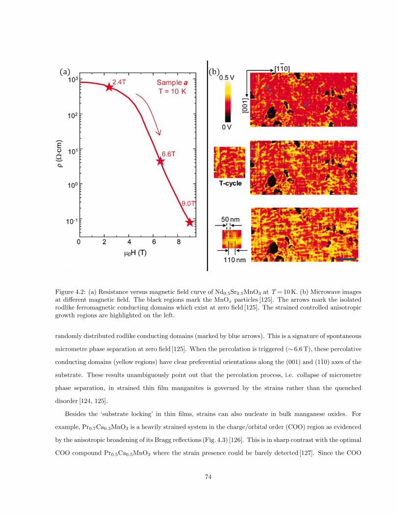
Figure 4.2: (a) Resistance versus magnetic field curve of Nd0.5Sr0.5MnO3 at T = 10 K. (b) Microwave imagesat different magnetic field. The black regions mark the MnOx particles [125]. The arrows mark the isolatedrodlike ferromagnetic conducting domains which exist at zero field [125]. The strained controlled anisotropicgrowth regions are highlighted on the left.
randomly distributed rodlike conducting domains (marked by blue arrows). This is a signature of spontaneous
micrometre phase separation at zero field [125]. When the percolation is triggered (∼ 6.6 T), these percolative
conducting domains (yellow regions) have clear preferential orientations along the (001) and (110) axes of the
substrate. These results unambiguously point out that the percolation process, i.e. collapse of micrometre
phase separation, in strained thin film manganites is governed by the strains rather than the quenched
disorder [124, 125].
Besides the ‘substrate locking’ in thin films, strains can also nucleate in bulk manganese oxides. For
example, Pr0.7Ca0.3MnO3 is a heavily strained system in the charge/orbital order (COO) region as evidenced
by the anisotropic broadening of its Bragg reflections (Fig. 4.3) [126]. This is in sharp contrast with the optimal
COO compound Pr0.5Ca0.5MnO3 where the strain presence could be barely detected [127]. Since the COO
74
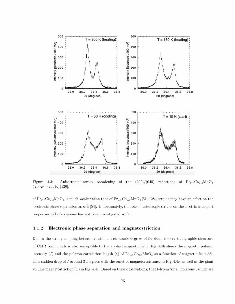
Figure 4.3: Anisotropic strain broadening of the (202)/(040) reflections of Pr0.7Ca0.3MnO3
(TCOO≈ 200 K) [126].
of Pr0.7Ca0.3MnO3 is much weaker than that of Pr0.5Ca0.5MnO3 [51, 128], strains may have an effect on the
electronic phase separation as well [54]. Unfortunately, the role of anisotropic strains on the electric transport
properties in bulk systems has not been investigated so far.
4.1.2 Electronic phase separation and magnetostriction
Due to the strong coupling between elastic and electronic degrees of freedom, the crystallographic structure
of CMR compounds is also susceptible to the applied magnetic field. Fig. 4.4b shows the magnetic polaron
intensity (I ) and the polaron correlation length (ξ) of La0.5Ca0.5MnO3 as a function of magnetic field [58].
This sudden drop of I around 3 T agrees with the onset of magnetoresistance in Fig. 4.4c, as well as the giant
volume magnetostriction (ω) in Fig. 4.4c. Based on these observations, the Holstein ‘small polarons’, which are
75
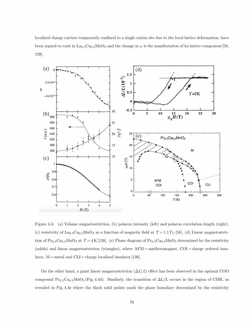
localized charge carriers temporarily confined to a single cation site due to the local lattice deformation, have
been argued to exist in La0.5Ca0.5MnO3 and the change in ω is the manifestation of its lattice component [58,
129].
Figure 4.4: (a) Volume magnetostriction, (b) polaron intensity (left) and polaron correlation length (right),
(c) resistivity of La0.5Ca0.5MnO3 as a function of magnetic field at T = 1.1TC [58]. (d) Linear magnetostric-
tion of Pr0.5Ca0.5MnO3 at T = 4 K [128]. (e) Phase diagram of Pr0.5Ca0.5MnO3 determined by the resistivity
(solids) and linear magnetostriction (triangles), where AFM = antiferromagnet, COI = charge ordered insu-
lator, M = metal and CLI = charge localized insulator [130].
On the other hand, a giant linear magnetostriction (∆L/L) effect has been observed in the optimal COO
compound Pr0.5Ca0.5MnO3 (Fig. 4.4d). Similarly, the transition of ∆L/L occurs in the region of CMR, as
revealed in Fig. 4.4e where the black solid points mark the phase boundary determined by the resistivity
76
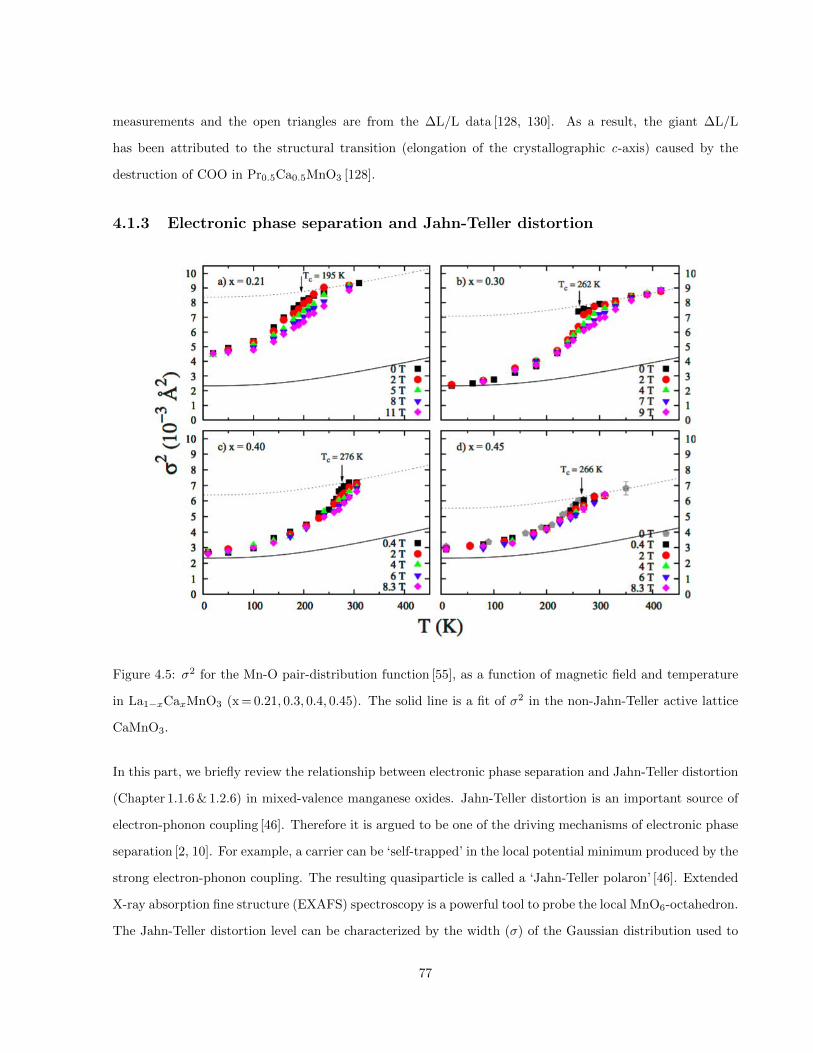
measurements and the open triangles are from the ∆L/L data [128, 130]. As a result, the giant ∆L/L
has been attributed to the structural transition (elongation of the crystallographic c-axis) caused by the
destruction of COO in Pr0.5Ca0.5MnO3 [128].
4.1.3 Electronic phase separation and Jahn-Teller distortion
Figure 4.5: σ2 for the Mn-O pair-distribution function [55], as a function of magnetic field and temperature
in La1−xCaxMnO3 (x = 0.21, 0.3, 0.4, 0.45). The solid line is a fit of σ2 in the non-Jahn-Teller active lattice
CaMnO3.
In this part, we briefly review the relationship between electronic phase separation and Jahn-Teller distortion
(Chapter 1.1.6 & 1.2.6) in mixed-valence manganese oxides. Jahn-Teller distortion is an important source of
electron-phonon coupling [46]. Therefore it is argued to be one of the driving mechanisms of electronic phase
separation [2, 10]. For example, a carrier can be ‘self-trapped’ in the local potential minimum produced by the
strong electron-phonon coupling. The resulting quasiparticle is called a ‘Jahn-Teller polaron’ [46]. Extended
X-ray absorption fine structure (EXAFS) spectroscopy is a powerful tool to probe the local MnO6-octahedron.
The Jahn-Teller distortion level can be characterized by the width (σ) of the Gaussian distribution used to
77

Figure 4.6: (a)The field dependence of σ2 (open circles) and magnetization (solids) of La0.5Ca0.5MnO3 [132].(b)-(d) The field dependence of the ferromagnetic, antiferromagnetic and COO Bragg reflections ofPr0.7Ca0.3MnO3, respectively [122].
fit the data [55, 131]. Fig. 4.5 demonstrates the evolution of σ2 by varying both temperature and magnetic
field in the ferromagnetic lanthanide compounds La1−xCaxMnO3 (x = 0.21, 0.3, 0.4, 0.45) where the CMR
occurs around TC [55, 2]. All samples are significantly distorted in the paramagnetic region. On further
cooling, σ2 is greatly suppressed when ferromagnetism sets in (T <TC). Similarly, applying a magnetic field
is also able to suppress the Jahn-Teller distortion. For the other family of CMR compounds with COO,
the field dependence of Jahn-Teller distortion has also been investigated. As shown in Fig. 4.6a, the sudden
increase in magnetization of La0.5Ca0.5MnO3 is accompanied by the decrease of the distortion parameter
σ2 =< (R − R)2 >, where R is the Mn-O bond length and R is the average Mn-O bond length [132]. Since
this type of metamagnetic transition is a common signature of COO melting (Fig. 4.6b-d) [122], these results
78
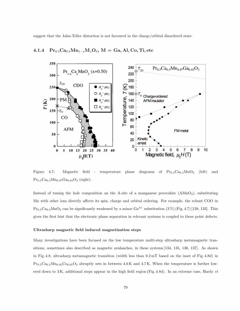
suggest that the Jahn-Teller distortion is not favoured in the charge/orbital disordered state.
4.1.4 Pr0.5Ca0.5Mn1−xMxO3, M = Ga, Al, Co, Ti, etc
Figure 4.7: Magnetic field - temperature phase diagrams of Pr0.5Ca0.5MnO3 (left) and
Pr0.5Ca0.5Mn0.97Ga0.03O3 (right).
Instead of tuning the hole composition on the A-site of a manganese perovskite (AMnO3), substituting
Mn with other ions directly affects its spin, charge and orbital ordering. For example, the robust COO in
Pr0.5Ca0.5MnO3 can be significantly weakened by a minor Ga3+ substitution (3 %) (Fig. 4.7) [128, 133]. This
gives the first hint that the electronic phase separation in relevant systems is coupled to these point defects.
Ultrasharp magnetic field induced magnetization steps
Many investigations have been focused on the low temperature multi-step ultrasharp metamagnetic tran-
sitions, sometimes also described as magnetic avalanches, in these systems [134, 135, 136, 137]. As shown
in Fig. 4.8, ultrasharp metamagnetic transition (width less than 0.2 mT based on the inset of Fig. 4.8d) in
Pr0.5Ca0.5Mn0.95Co0.05O3 abruptly sets in between 4.6 K and 4.7 K. When the temperature is further low-
ered down to 3 K, additional steps appear in the high field region (Fig. 4.8d). In an extreme case, Hardy et
79

al have shown that hundreds of magnetization steps can be realized by cooling Pr0.5Ca0.5Mn0.97Ga0.03O3
to 1.5 K [138]. Each step in magnetization corresponds to a sudden growth of ferromagnetism while the
CE (or pseudo-CE) type antiferromagnetic order in the sample is partially suppressed [139, 127]. Since the
CE (or pseudo-CE) type antiferromagnetic order in manganites couples tightly with the orbital degree of
freedom [2, 122, 52], this antiferro-ferromagnetic transition is also accompanied by a cooperative change of
the local lattice distortion, as discussed in the previous section. This sort of diffusionless structure change
in manganites is the analogue of the martensite-austenite transformation in alloys [138, 140]. As a result, a
martensitic scenario, in which the spin related energy (e.g. exchange interactions, Zeeman energy) is compet-
ing with the elastic energy associated with the strains at the antiferromagnetic/ferromagnetic interfaces, has
been proposed to quantitatively understand these magnetic avalanches. In this scenario, the spins are locked
by these strains at low fields so that the bulk magnetization is not sensitive to magnetic field. However, a
sudden growth of ferromagnetism will be promoted once these spins are unlocked by magnetic field.
Figure 4.8: a-d, Magnetic field versus magnetization curves of Pr0.5Ca0.5Mn0.95Co0.05O3 under various con-
ditions. FC = field cool, ZFC = zero field cool.
80

Anisotropic strains and crystallographic phase separation
Figure 4.9: Selected region of the synchrotron X-ray powder diffraction (λ= 0.500111(12) A) patterns of
Pr0.5Ca0.5Mn0.97Ti0.03O3 [127] at (a) room temperature and (b) 5 K. Two crystallographic phases are needed
to fit all the Bragg reflections at 5 K. (c) Temperature dependence of the lattice parameters (left) and the
volume fraction of each phase (space group Pnma). Phase-1: CE phase. Phase-2: pseudo-CE phase. (d)
Neutron powder diffraction patterns of Pr0.5Ca0.5Mn1−xTixO3.
The crystallographic structures of some Pr0.5Ca0.5Mn1−xMxO3 systems have been studied by the high-
resolution synchrotron X-ray diffraction technique [127, 141, 142]. In the charge/orbital ordered region, these
systems are found to be strongly strained. The presence of anisotropic strains will broaden the corresponding
81

Bragg reflections (Fig. 4.9b), which can be described by the Stephens formalism [143]:
σ2hkl =
H+K+L=4∑H,K,L
SHKLhHkK lL, (4.1)
where σ2hkl is the broadening of the (h, k, l) reflection and SHKL are the parameters refined from the peak
shape [102, 106]. For the Pr0.5Ca0.5Mn1−xMxO3 compounds with an orthorhombic unit cell, this equation
reduces to six non-zero terms:
σ2hkl = S400h
4 + S040k4 + S004l
4 + S220h2k2 + S202h
2l2 + S022k2l2. (4.2)
As an example, the X-ray diffraction patterns of Pr0.5Ca0.5Mn0.97Ti0.03O3 above and below the COO
temperature (∼ 240 K), measured by Garcıa-Munoz et al [127], have been displayed in Fig. 4.9a-b. At room
temperature, the pattern can be refined within a single phase approach and the strain broadening parameters
are negligible (Table. 4.1). In sharp contrast, these Bragg peaks are significantly broadened at 5 K. Moreover,
there are more than four peaks in this region, meaning the single phase approach is not enough to match all
these peaks. Alternatively, a two phase approach is able to capture all these features (Fig. 4.9b). Indeed, the
crystallographic phase separation picture is required to explain the coexistence of CE and pseudo-CE anti-
ferromagnetic phases in this compound revealed by the neutron powder diffraction measurements (Fig. 4.9d).
Table 4.1: Volume fractions, unit cell distortions (D) and strain parameters of Pr0.5Ca0.5Mn0.97Ti0.03O3 [127].
Fraction D S400 S040 S004 S220 S202 S022
Room temperature 100 % 0.997 0.178(3) 0.087(1) 0.160(6) -0.134(5) 0.89(1) -0.165(7)
5 K (CE) 55 % 0.9764 0.175(9) 0.239(4) 0.33(1) -0.02(2) 1.32(3) -0.02(2)
5 K (pseudo-CE) 45 % 0.9855 2.17(6) 3.02(6) 4.3(1) -2.9(1) 7.8(2) -4.5(2)
Besides the Jahn-Teller distortion which is related to the MnO6-octahedron, the distortion of the unit
cell can be charaterized by a parameter D =
√2b
a + c(with space group Pnma). An undistorted lattice
would have D = 1, where D 6= 1 in distorted cases [127, 141, 142]. As shown in Table. 4.1, the unit cell of
Pr0.5Ca0.5Mn0.97Ti0.03O3 is almost undistorted at room temperature, whereas both CE and pseudo-CE
phases are highly distorted at 5 K. It is worth noting that the CE phase in all Pr0.5Ca0.5Mn1−xMxO3
compounds has a more distorted unit cell than the pseudo-CE phase. This is also consistent with the
Pr1−xCaxMnO3 family [50]. Most of all, COO in both families seems to correlate with D, i.e. the unit
82

cell distortion tends to stabilize COO [51, 128, 127, 139]. As a result, the COO in the CE phase is more
robust than that of the pseudo-CE phases, which is responsible for the two-step metamagnetic transition
phenomenon observed in these systems [133, 135]. Specifically, the low field transition is due to the COO
melting in the pseudo-CE phase, while higher magnetic field is needed to suppress the COO in the CE phase.
We also emphasize that the less distorted pseudo-CE phase is transforming into the CE phase as tempera-
ture is lowered (Fig. 4.9c). On the other hand, the pseudo-CE nuclear lattice is much more strained compared
with the CE nuclear lattice (Table. 4.1). This may be caused by the inhomogeneous distribution of M ions in
the sample, as stated in Ref. [127].
4.2 Results
4.2.1 Research motivations
In general, by equipping small angle neutron scattering (SANS) and time-of-flight neutron powder diffraction
(TOF-NPD) techniques with state-of-the-art sample environments, we want to monitor the evolution of
the multiple scale phase separation by varying the magnetic field; as well as check their coupling to the
crystallographic lattice. Based on the previous studies, the spin degree of freedom seems to be indispensable
to the carrier delocalization [10, 60, 61, 58, 121, 57, 122], whereas DE is not the driving force of the carrier
localization in CMR manganites [2, 10, 46]. On the other hand, spins can be locked by strains through
magnetoelastic coupling [138]. To our knowledge, the correlation between DE and carrier delocalization in a
strained manganite has not been studied to date.
On the other hand, the giant volume (linear) magnetostriction observed in manganese perovskites has
been associated with the collapse of electronic phases such as polarons and COO (Fig. 4.4). This scenario
has never been verified using the diffraction technique, which directly probes the lattice parameters of the
unit cell. Instead, most of the microscopic structure investigations performed in the past have focused on the
local Jahn-Teller distortion. All these measurements suggest that the Jahn-Teller distortion in manganese
perovskites is weakened by magnetic field across the melting of polarons (COO) (Fig. 4.5 & 4.6).
Besides the magnetism and electric transport properties, the orbital physics is another key concept in
transition-metal oxides [52]. For the CMR compounds, an orbital order populates when the system is an
insulator [2, 10]. However, the orbital arrangement in the metallic region remains an open question so far.
Even in the metallic region, a large fraction of localized carriers should still survive due to the low electric
conductivity of the ‘bad metal’ [2, 144, 145]. These localized carriers are expected to promote some sort of
83

orbital arrangement such as orbital order or orbital liquid [52]. For example, Cepas et al have suggested a
dx2−y2 type orbital order may be stabilised by magnetic field in the half-doped manganites where the zero
field orbital order is d3x2−r2/d3y2−r2 type [146]. However, magnetic field induced orbital order has never
been observed in these systems. Among all the factors, Jahn-Teller distortion is the key to understand the
nature of orbital order. First of all, the crystal field splitting, which correlates with the electron-phonon
coupling strength λ (Chapter 1.2.6), is determined by the amplitude of Jahn-Teller distortion. This means a
larger Jahn-Teller distortion corresponds to more localized charge carriers [2, 47]. Secondly, the Jahn-Teller
distortion mode is responsible for the symmetry of the active eg orbital [10].
In summary, we are trying to answer the following three questions by carrying out this research project:
1. Does DE couple to the carrier delocalization in a strained manganite?
2. Is the collapse of electronic phase separation responsible for the giant magnetostriction effect in a
strained manganite?
3. What is the magnetic field dependences of the Jahn-Teller distortion in a strained manganite?
4.2.2 Data analysis
Time-of-flight neutron powder diffraction
The patterns obtained from TOF-NPD measurements have been analyzed using the Rietveld method de-
scribed in Appendix A. In this part, we will use the patterns taken at T = 150 K/B = 0 T and T = 150 K/B = 10 T
as an example to show the general refinement procedure. We have chosen the space group Pnma to describe
the crystallographic structure of Pr0.5Ca0.5Mn0.97Ga0.03O3 (PCMGO) [139]. For the TOF-NPD pattern, the
convolution pseudo-Voigt with back-to-back exponential functions are required to fit the profiles of the Bragg
reflections [106, 147]. The instrumental resolution parameters were obtained by measuring the standard
Na2Ca3Al2F14 sample. For the pseudo-CE phase, these parameters have been fixed and only the 6 strain
parameters (Stephens formalism [143]) were allowed to vary during the refinement. For the CE phase, it is
much less strained and only occupy a minor fraction at high temperatures [127, 141, 142, 139]. As a result,
only the Gaussian component Sig-2 was refined to fit the peak profiles [106, 147]. A third phase, coming from
the Al-holder has been treated properly using the LeBail method [148].
84
In this paragraph, only the sloping background at small d-spacings has been fitted. As discussed in
Ref. [127, 141, 142, 139], Pr0.5Ca0.5Mn0.97Ga0.03O3 demonstrate crystallographic phase separation in the
COO region (T <∼ 240 K). However, the more distorted CE phase has a very low volume fraction at high
temperatures (Fig. 4.9c). Since the TOF-NPD technique does not have as high resolution as the synchrotron
X-ray diffraction, it is reasonable to check whether this minority CE phase can be resolved at 150 K. The re-
fined pattern using a 1-phase model is shown in Fig. 4.10a. Although the overall fitting quality is satisfactory,
it is clear that the peak intensities around 2.70 A (3.82 A) have been under- (over-) estimated. On the other
hand, the 2-phase refinement produces much better profiles to match these peaks (Fig. 4.10b). The refined
lattice parameters, atomic positions, strain parameters and phase fractions are listed in Table 4.2.
85
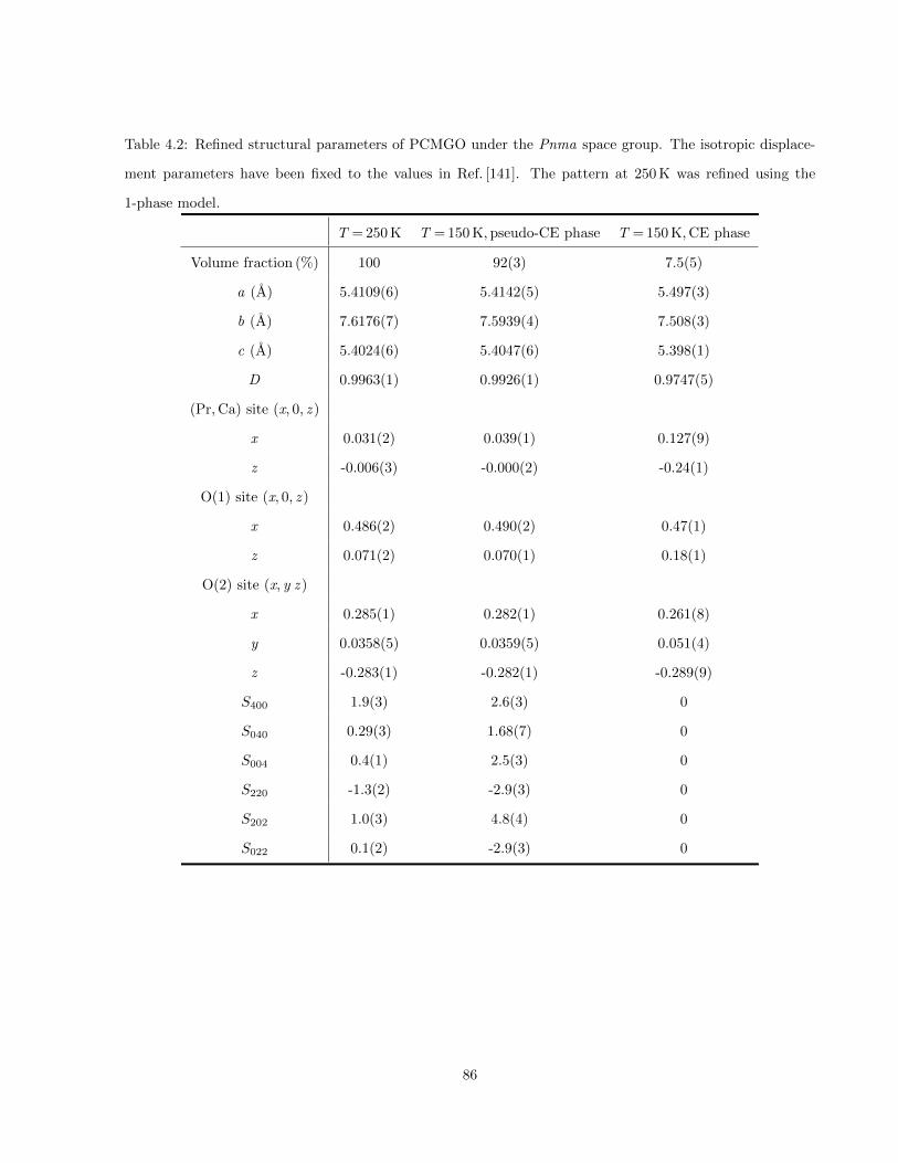
Table 4.2: Refined structural parameters of PCMGO under the Pnma space group. The isotropic displace-
ment parameters have been fixed to the values in Ref. [141]. The pattern at 250 K was refined using the
1-phase model.
T = 250 K T = 150 K, pseudo-CE phase T = 150 K, CE phase
Volume fraction (%) 100 92(3) 7.5(5)
a (A) 5.4109(6) 5.4142(5) 5.497(3)
b (A) 7.6176(7) 7.5939(4) 7.508(3)
c (A) 5.4024(6) 5.4047(6) 5.398(1)
D 0.9963(1) 0.9926(1) 0.9747(5)
(Pr, Ca) site (x, 0, z )
x 0.031(2) 0.039(1) 0.127(9)
z -0.006(3) -0.000(2) -0.24(1)
O(1) site (x, 0, z )
x 0.486(2) 0.490(2) 0.47(1)
z 0.071(2) 0.070(1) 0.18(1)
O(2) site (x, y z )
x 0.285(1) 0.282(1) 0.261(8)
y 0.0358(5) 0.0359(5) 0.051(4)
z -0.283(1) -0.282(1) -0.289(9)
S400 1.9(3) 2.6(3) 0
S040 0.29(3) 1.68(7) 0
S004 0.4(1) 2.5(3) 0
S220 -1.3(2) -2.9(3) 0
S202 1.0(3) 4.8(4) 0
S022 0.1(2) -2.9(3) 0
86
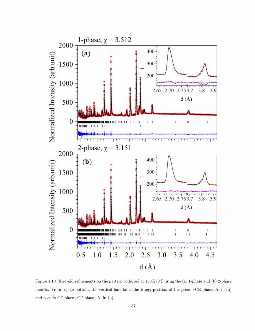
Figure 4.10: Rietveld refinements on the pattern collected at 150 K/0 T using the (a) 1-phase and (b) 2-phase
models. From top to bottom, the vertical bars label the Bragg position of the pseudo-CE phase, Al in (a)
and pseudo-CE phase, CE phase, Al in (b).
87
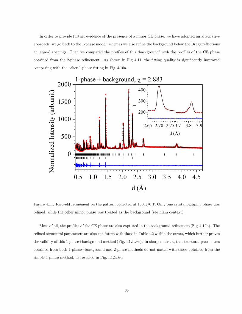
In order to provide further evidence of the presence of a minor CE phase, we have adopted an alternative
approach: we go back to the 1-phase model, whereas we also refine the background below the Bragg reflections
at large-d spacings. Then we compared the profiles of this ‘background’ with the profiles of the CE phase
obtained from the 2-phase refinement. As shown in Fig. 4.11, the fitting quality is significantly improved
comparing with the other 1-phase fitting in Fig. 4.10a.
Figure 4.11: Rietveld refinement on the pattern collected at 150 K/0 T. Only one crystallographic phase was
refined, while the other minor phase was treated as the background (see main context).
Most of all, the profiles of the CE phase are also captured in the background refinement (Fig. 4.12b). The
refined structural parameters are also consistent with those in Table 4.2 within the errors, which further proves
the validity of this 1-phase+background method (Fig. 4.12a &c). In sharp contrast, the structural parameters
obtained from both 1-phase+background and 2-phase methods do not match with those obtained from the
simple 1-phase method, as revealed in Fig. 4.12a &c.
88

Figure 4.12: (a) and (c) Comparisom of the structural parameters obtained from the 3 different methods
discussed in the main context. (b) The CE-phase profiles, corresponding to d ' 2.7 A, extracted from the
2-phase (red) and 1-phase+background (black) methods.
The 1-phase+background method used at zero magnetic field can be extended to the high field refinements.
Since the nuclear Bragg reflections at large d-spacings will be superimposed by the strong ferromagnetic
signals in the ferromagnetic region, it would be very hard to refine the minor CE phase. Moreover, the CE
COO has been proven to be more robust against the magnetic field than the pseudo-CE COO [51, 128, 139,
127]. This leads to a two-step metamagnetic transition in the Pr0.5Ca0.5Mn1−xMxO3 family [133, 135]. Based
on our estimation, we should still be able to resolve the ferromagnetic transition caused by the minor CE COO
melting as long as we can reach the corresponding critical field. However, the second metamagnetic transition,
which is associated with the collapse of CE COO, is much smoother compared with the one in the low field
region [133, 135]. This continuous feature may further prohibit us from observing the CE COO melting.
Since we shall mainly focus on the majority pseudo-CE phase here, the 1-phase+background treatment is a
more suitable choice. If the critical field of CE COO melting is beyond our reach in experiments, such ‘CE
background’ would not change with the varying field. On the other hand, any continuous or discontinuous
89
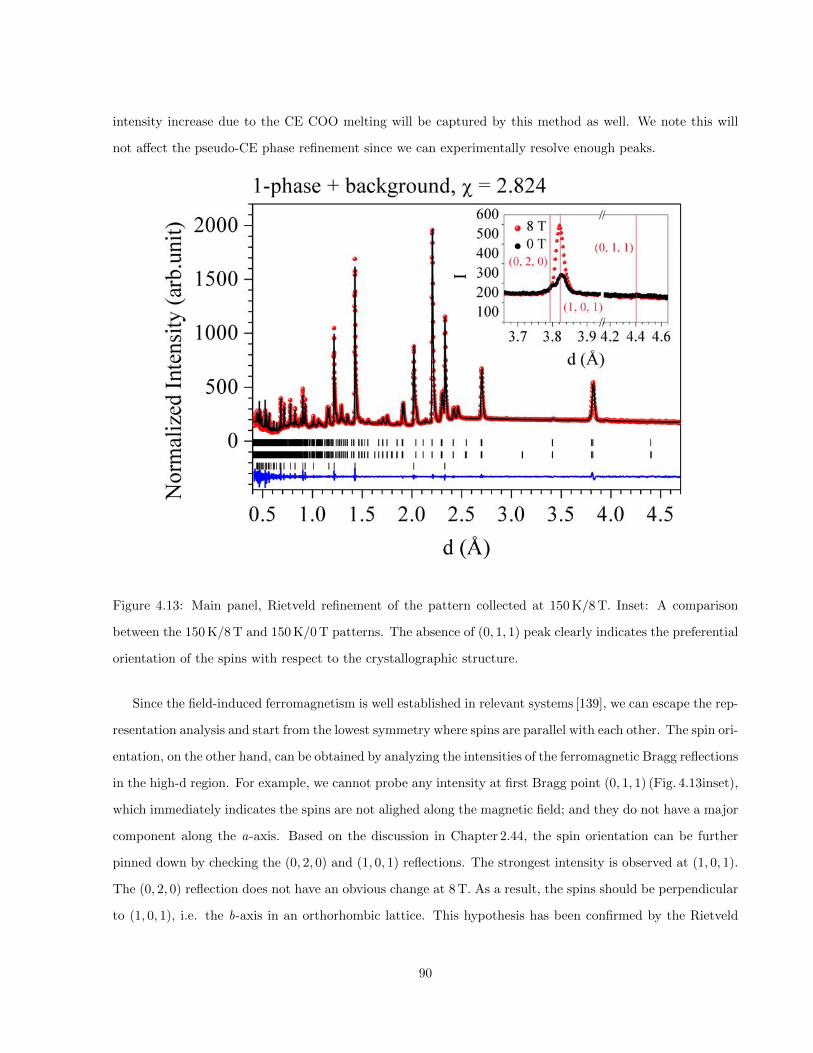
intensity increase due to the CE COO melting will be captured by this method as well. We note this will
not affect the pseudo-CE phase refinement since we can experimentally resolve enough peaks.
Figure 4.13: Main panel, Rietveld refinement of the pattern collected at 150 K/8 T. Inset: A comparison
between the 150 K/8 T and 150 K/0 T patterns. The absence of (0, 1, 1) peak clearly indicates the preferential
orientation of the spins with respect to the crystallographic structure.
Since the field-induced ferromagnetism is well established in relevant systems [139], we can escape the rep-
resentation analysis and start from the lowest symmetry where spins are parallel with each other. The spin ori-
entation, on the other hand, can be obtained by analyzing the intensities of the ferromagnetic Bragg reflections
in the high-d region. For example, we cannot probe any intensity at first Bragg point (0, 1, 1) (Fig. 4.13inset),
which immediately indicates the spins are not alighed along the magnetic field; and they do not have a major
component along the a-axis. Based on the discussion in Chapter 2.44, the spin orientation can be further
pinned down by checking the (0, 2, 0) and (1, 0, 1) reflections. The strongest intensity is observed at (1, 0, 1).
The (0, 2, 0) reflection does not have an obvious change at 8 T. As a result, the spins should be perpendicular
to (1, 0, 1), i.e. the b-axis in an orthorhombic lattice. This hypothesis has been confirmed by the Rietveld
90
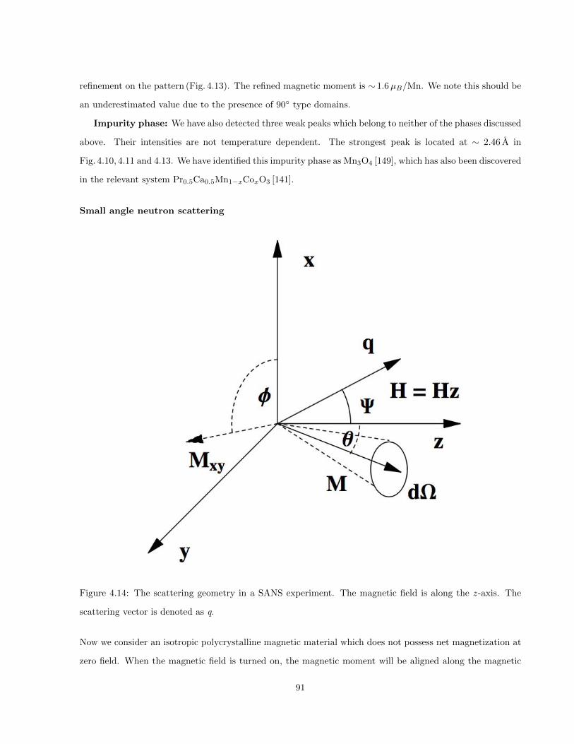
refinement on the pattern (Fig. 4.13). The refined magnetic moment is ∼ 1.6µB/Mn. We note this should be
an underestimated value due to the presence of 90 type domains.
Impurity phase: We have also detected three weak peaks which belong to neither of the phases discussed
above. Their intensities are not temperature dependent. The strongest peak is located at ∼ 2.46 A in
Fig. 4.10, 4.11 and 4.13. We have identified this impurity phase as Mn3O4 [149], which has also been discovered
in the relevant system Pr0.5Ca0.5Mn1−xCoxO3 [141].
Small angle neutron scattering
Figure 4.14: The scattering geometry in a SANS experiment. The magnetic field is along the z -axis. The
scattering vector is denoted as q.
Now we consider an isotropic polycrystalline magnetic material which does not possess net magnetization at
zero field. When the magnetic field is turned on, the magnetic moment will be aligned along the magnetic
91
field. Provided that the 2-dimensional detector is always perpendicular to the direct beam (Fig. 2.6) and the
neutrons are only sensitive to the magnetic moment perpendicular to q, the intensity detected at a wavevector
transfer q can be writen as
I(q,Ψ) = IA (q) + IB (q) sin2Ψ, (4.3)
where Ψ is the angle between the magnetic field and q (Fig. 4.14), IA (q) contains the isotropic nuclear
scattering signal as well as the magnetic scattering signal from the spins not aligned by the magnetic field,
IB (q) sin2Ψ is the pure magnetic signal from the spins aligned by the magnetic field [150, 151, 152].
We have covered a wide q range from 2.2× 10⁻³ A−1 to 0.23 A−1 in our experiments. This enables us to
monitor the magnetic field dependence of micrometre and electronic phase separation simultaneously. For
the micrometre phases, they can be described by the modified Porod’s equation:
Im (q) = 2π(∆ρm)2(S
V)mq
−4exp(−q2σ2m), (4.4)
where (∆ρm)2 is the magnetic contrast, (S
V)m is the magnetic specific nonferromagnetic/ferromagnetic in-
terface parameter which is related to the domain dynamics, σm is the half width of the magnetic interface
profile [153]. On the other hand, the magnetic polarons can be treated as atomic scale inhomogeneities using
a Lorentzian function
Ip (q) = I0ξ2
1 + q2ξ2, (4.5)
where ξ is the characteristic size of these polarons [58]. We have also observed the incommensurate orbital
order at zero field [154]. As a result, an additional Gaussian term is required
IOO = Aexp(−(q − qc)2
2W 2)/W√
2π, (4.6)
where qc is the center of the peak, A is the area, W is the width. Finally, another Porod’s equation is used
to describe the nuclear scattering [152]
Inuc (q) = 2π(∆ρnuc)2(S
V)nucq
−4exp(−q2σ2nuc). (4.7)
Most of the data discussed in this thesis were collected using a 17-Tesla horizontal magnet [155]. This
means the magnetic field is always perpendicular to q so that the scattering pattern should be isotropic based
92

on eq. 4.3. As a result, the total intensity I (q) was obtained by summing all the intensities at the same q point
in the 2D detector. We used three different instrumental configurations to cover the wide q range (2.2× 10⁻³ A
to 0.23 A). As discussed in Chapter 2.5, q is a function of the scattering angle θ and the wavlength λ. In
practice, θ can be tuned by changing the distance between the sample and detector (L) (Fig. 2.6). In order to
cover the required q range, both L and λ can be modified. Experimentally, we are only counting the number
of neutrons instead of directly measuring the scattering cross-section. This means the intensities need to be
normalized into absolute units (cm−1) in order to merge the three patterns (Fig. 4.15) [156].
Iabs (q) =I (q)
Φ0 TrΩ (q) t d, (4.8)
where Φ0 is the incident neutron flux, Tr is the transmission, Ω (q) is the solid angle at q, t is the measuring
time and d is the thickness of the sample [156].
Figure 4.15: T = 150 K, B = 2 T. (a) I (q)-q curves under different instrumental configurations. (b) The
merged curve. The shaded areas mark the overlapping regions.
Unfortunately, we did not measure the transmission parameters properly during the experiment. A slight
rescaling has been applied to the data after treatment using eq. 4.8 (Fig. 4.15b). We note this additional
treatment does not affect the absolute values of the parameters in the exponential brackets in eq. 4.4 - eq. 4.7.
Although the values of other parameters, e.g. the magnetic specific interface (S
V)m, will not have any physical
meaning, their field dependence still reflects the physics of the sample.
We will use the I (q) versus q curve collected at 150 K/2 T to demonstrate the data analysis process.
93

Under the horizontal field setup, we fit the experimental curve by
I (q) = Im + Ip + IOO + Inuc. (4.9)
As shown in Fig. 4.16a, this model is able to fit the experimental data quite well. More importantly, it is clear
each term has its own active region. For example, the intensity in the very low-q region is dominated by the
nuclear scattering. This is expected since the object size is proportional to q−1 and the crystalline grains are
normally on micrometre scales. For the incommensurate orbital order and polarons, we will discuss them in
the next subsection.
Figure 4.16: (a) I (q) versus q curve at 150 K/2 T under the horizontal field setup and the simulated contri-
butions using eq. 4.9. (b) I (q) versus q curve at 150 K/10 T under the vertical field setup and the simulated
contributions using eq. 4.7.
We have also used a vertical field setup (11-Tesla magnet) to double check the validity of the Inuc term.
In this case, the magnetic field is parallel to qx, i.e. horizontal direction in the 2D detector. According to
eq. 4.3, the intensity along qx (Ψ = 0) should exclusively contain the nuclear scattering signal when the spins
are aligned. As depicted in Fig. 4.16b, the Porod’s term Inuc is able to fully reproduce the experimental
observations.
In conclusion, we have demonstrated that eq. 4.9 is a very good model to fit the experimental data under
the horizontal field setup.
94
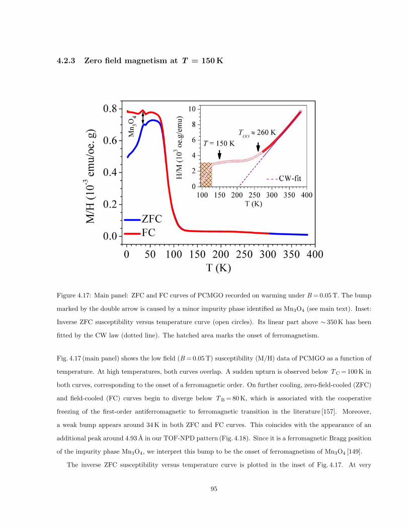
4.2.3 Zero field magnetism at T = 150 K
Figure 4.17: Main panel: ZFC and FC curves of PCMGO recorded on warming under B = 0.05 T. The bump
marked by the double arrow is caused by a minor impurity phase identified as Mn3O4 (see main text). Inset:
Inverse ZFC susceptibility versus temperature curve (open circles). Its linear part above ∼ 350 K has been
fitted by the CW law (dotted line). The hatched area marks the onset of ferromagnetism.
Fig. 4.17 (main panel) shows the low field (B = 0.05 T) susceptibility (M/H) data of PCMGO as a function of
temperature. At high temperatures, both curves overlap. A sudden upturn is observed below TC = 100 K in
both curves, corresponding to the onset of a ferromagnetic order. On further cooling, zero-field-cooled (ZFC)
and field-cooled (FC) curves begin to diverge below TB = 80 K, which is associated with the cooperative
freezing of the first-order antiferromagnetic to ferromagnetic transition in the literature [157]. Moreover,
a weak bump appears around 34 K in both ZFC and FC curves. This coincides with the appearance of an
additional peak around 4.93 A in our TOF-NPD pattern (Fig. 4.18). Since it is a ferromagnetic Bragg position
of the impurity phase Mn3O4, we interpret this bump to be the onset of ferromagnetism of Mn3O4 [149].
The inverse ZFC susceptibility versus temperature curve is plotted in the inset of Fig. 4.17. At very
95
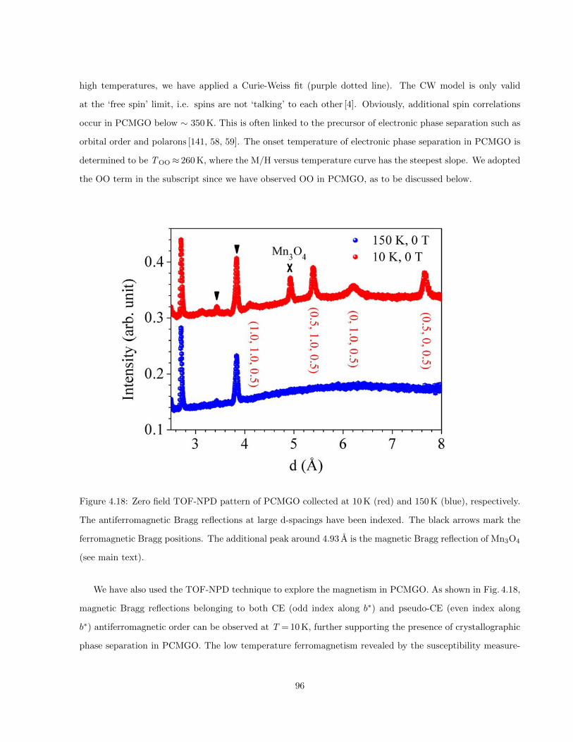
high temperatures, we have applied a Curie-Weiss fit (purple dotted line). The CW model is only valid
at the ‘free spin’ limit, i.e. spins are not ‘talking’ to each other [4]. Obviously, additional spin correlations
occur in PCMGO below ∼ 350 K. This is often linked to the precursor of electronic phase separation such as
orbital order and polarons [141, 58, 59]. The onset temperature of electronic phase separation in PCMGO is
determined to be TOO≈ 260 K, where the M/H versus temperature curve has the steepest slope. We adopted
the OO term in the subscript since we have observed OO in PCMGO, as to be discussed below.
Figure 4.18: Zero field TOF-NPD pattern of PCMGO collected at 10 K (red) and 150 K (blue), respectively.
The antiferromagnetic Bragg reflections at large d-spacings have been indexed. The black arrows mark the
ferromagnetic Bragg positions. The additional peak around 4.93 A is the magnetic Bragg reflection of Mn3O4
(see main text).
We have also used the TOF-NPD technique to explore the magnetism in PCMGO. As shown in Fig. 4.18,
magnetic Bragg reflections belonging to both CE (odd index along b∗) and pseudo-CE (even index along
b∗) antiferromagnetic order can be observed at T = 10 K, further supporting the presence of crystallographic
phase separation in PCMGO. The low temperature ferromagnetism revealed by the susceptibility measure-
96
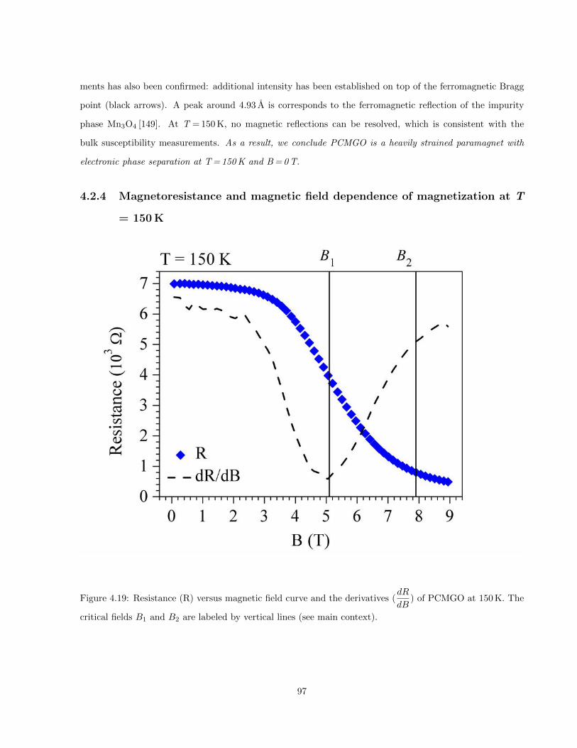
ments has also been confirmed: additional intensity has been established on top of the ferromagnetic Bragg
point (black arrows). A peak around 4.93 A is corresponds to the ferromagnetic reflection of the impurity
phase Mn3O4 [149]. At T = 150 K, no magnetic reflections can be resolved, which is consistent with the
bulk susceptibility measurements. As a result, we conclude PCMGO is a heavily strained paramagnet with
electronic phase separation at T = 150 K and B = 0 T.
4.2.4 Magnetoresistance and magnetic field dependence of magnetization at T
= 150 K
Figure 4.19: Resistance (R) versus magnetic field curve and the derivatives (dR
dB) of PCMGO at 150 K. The
critical fields B1 and B2 are labeled by vertical lines (see main context).
97

Figure 4.20: Main panel: Magnetization versus magnetic field curve (red line) of PCMGO at 150 K. The
black arrows mark the field sweeping direction. The blue line is a linear fit to the low field part where the
system is paramagnetic. The critical fields B1 and B2 are labeled by vertical lines (see main context). Inset:
Enlarged version of the shaded area in the main panel.
After determining the zero field state of PCMGO at T = 150 K, the next step is to switch on the magnetic
field. As shown in Fig. 4.19, the resistance (R) undergoes a large drop in the high magnetic field (B) region.
This magnetoresistance curve has the steepest slope at B1 = 5.1 T. The transition at B1 is often linked to
the melting of electronic phase separation in literatures [58, 51, 122]. For the PCMGO case, the microscopic
nature of the transition at B1 will be discussed in the next subsection. Since the melting of electronic
phase separation (e.g. orbital order) is also accompanied by the onset of ferromagnetism in other relevant
compounds [122], we have explored the bulk magnetization (M ) as a function of B in Fig. 4.20. The M -B
curve is linear at low fields, indicating that PCMGO is still paramagnetic. Further increasing B results in a
98
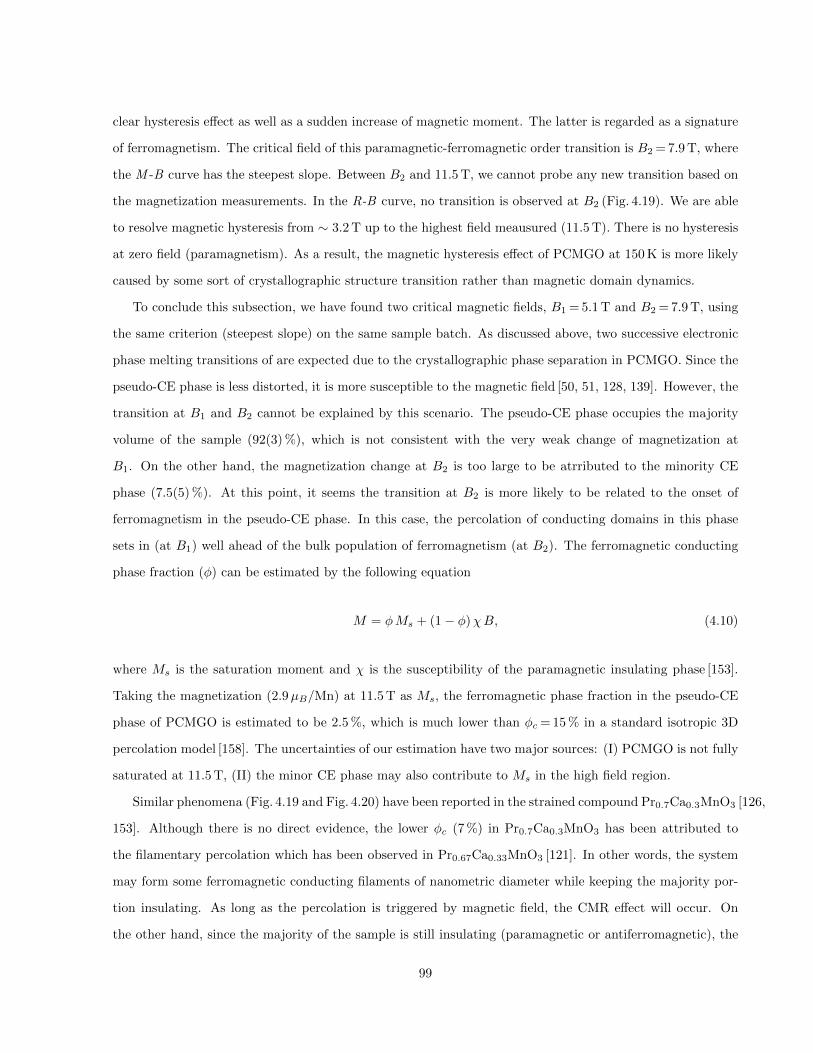
clear hysteresis effect as well as a sudden increase of magnetic moment. The latter is regarded as a signature
of ferromagnetism. The critical field of this paramagnetic-ferromagnetic order transition is B2 = 7.9 T, where
the M -B curve has the steepest slope. Between B2 and 11.5 T, we cannot probe any new transition based on
the magnetization measurements. In the R-B curve, no transition is observed at B2 (Fig. 4.19). We are able
to resolve magnetic hysteresis from ∼ 3.2 T up to the highest field meausured (11.5 T). There is no hysteresis
at zero field (paramagnetism). As a result, the magnetic hysteresis effect of PCMGO at 150 K is more likely
caused by some sort of crystallographic structure transition rather than magnetic domain dynamics.
To conclude this subsection, we have found two critical magnetic fields, B1 = 5.1 T and B2 = 7.9 T, using
the same criterion (steepest slope) on the same sample batch. As discussed above, two successive electronic
phase melting transitions of are expected due to the crystallographic phase separation in PCMGO. Since the
pseudo-CE phase is less distorted, it is more susceptible to the magnetic field [50, 51, 128, 139]. However, the
transition at B1 and B2 cannot be explained by this scenario. The pseudo-CE phase occupies the majority
volume of the sample (92(3) %), which is not consistent with the very weak change of magnetization at
B1. On the other hand, the magnetization change at B2 is too large to be atrributed to the minority CE
phase (7.5(5) %). At this point, it seems the transition at B2 is more likely to be related to the onset of
ferromagnetism in the pseudo-CE phase. In this case, the percolation of conducting domains in this phase
sets in (at B1) well ahead of the bulk population of ferromagnetism (at B2). The ferromagnetic conducting
phase fraction (φ) can be estimated by the following equation
M = φMs + (1− φ)χB, (4.10)
where Ms is the saturation moment and χ is the susceptibility of the paramagnetic insulating phase [153].
Taking the magnetization (2.9µB/Mn) at 11.5 T as Ms, the ferromagnetic phase fraction in the pseudo-CE
phase of PCMGO is estimated to be 2.5 %, which is much lower than φc = 15 % in a standard isotropic 3D
percolation model [158]. The uncertainties of our estimation have two major sources: (I) PCMGO is not fully
saturated at 11.5 T, (II) the minor CE phase may also contribute to Ms in the high field region.
Similar phenomena (Fig. 4.19 and Fig. 4.20) have been reported in the strained compound Pr0.7Ca0.3MnO3 [126,
153]. Although there is no direct evidence, the lower φc (7 %) in Pr0.7Ca0.3MnO3 has been attributed to
the filamentary percolation which has been observed in Pr0.67Ca0.33MnO3 [121]. In other words, the system
may form some ferromagnetic conducting filaments of nanometric diameter while keeping the majority por-
tion insulating. As long as the percolation is triggered by magnetic field, the CMR effect will occur. On
the other hand, since the majority of the sample is still insulating (paramagnetic or antiferromagnetic), the
99

magnetization is not supposed to exhibit any large change across such percolation.
4.2.5 Collapse of electronic phase separation induced by magnetic field at T =
150 K
Figure 4.21: The magnetic field dependences of SANS patterns of PCMGO under the same scale (100 – 900
neutron counts per standard monitor). Each patterm covers a q-range from -0.2 A−1 to 0.2 A−1 in both
directions. The narrow vertical slit on the left of each pattern is coming from a dead detector tube.
Assuming the magnetoresistance of PCMGO is caused by the formation of conducting filaments in magnetic
field and the electronic phase separation (e.g. orbital order, polarons) is a bulk behaviour, the majority of the
sample will still be insulating, i.e. possessing electronic phase separation, between B1 and B2. The second
assumption should hold in all relevant CMR manganites since there is no evidence showing the electronic
phase separation is not a bulk behaviour to the best of our knowledge. For the specific PCMGO case, the
electron diffraction techique has been employed to search for the structure modulation caused by the electronic
100

phase separation [142, 159]. In most of the crystallites studied, they have observed extra diffraction spots
which are the characteristic signatures of charge/orbital order [142, 159].
As discussed above, PCMGO is paramagnetic at 150 K. In all the relevant compounds, e.g. PCMGO and
Pr1−xCaxMnO3, the orbital order is reported to be incommensurate in the paramagnetic region [142, 154,
159]. We have observed this incommensurate orbital order of PCMGO in our SANS measurements. Fig. 4.21
shows the field dependences of the SANS patterns after subtraction of the background data measured at
B = 16 T where the electronic phase separation is almost fully suppressed based on our qualitative analyses
(see the next paragraph). In the low field region, a ring-like pattern is observed. These corresponds to
a broad peak centered at ∼ 0.075 A−1. The ring intensity is relatively stable against magnetic field when
B 6 4 T. However, it is drastically suppressed between 4 T and 6 T. When B > 6 T, additional intensities start
to accumulate around the center of these patterns. These intensities are also field dependent. They represent
the scattering signals from the micrometre phases (eq. 4.4) rather than the electronic phases based on our
qualitative analyses (see the next paragraph).
We note that this type of background subtraction is only for quantitative demonstration. As shown
in eq. 4.4-eq. 4.7, there are additional contributions to the neutron scattering signals in the high-q region,
meaning the ‘background’ refered to above may also be field dependent! The best way to extract different
contributions out from the total scattering intensity is to fit the I-Q curves using eq. 4.9, as displayed in
Fig. 4.16. Fig. 4.22a shows the field dependence of the integrated intensity (IOO) of the incommensurate
orbital order peak. IOO is greatly suppressed between 4 T and 6 T, indicating the transition at B1 = 5.1 T is
caused by the melting of orbital order. Interestingly, a very weak peak centered at 0.04(1) A−1 is required
to fit the curves above 4 T. The intensity of this peak is temporarily enhanced between 6 T and 10 T (B3)
followed by a gradual decrease at higher fields up to 16 T. We attribute this peak to the incommensurate
orbital order in the minority CE phase. We have also detected the presence of atomic size clusters in PCMGO.
They are often linked to the size of magnetic polarons (carrier hopping range) [58]. The correlation length
(ξ) of these polarons as a function of magnetic field is plotted in Fig. 4.22b. Similar with the orbital order,
ξ also gives a big drop between 4 T and 6 T. While a weak enhancement is observed between 6 T and 8 T,
ξ is gradually suppressed above B3 as well. Fig. 4.22d plots the evolution of the magnetic specific interface
parameter (S/V) in magnetic field (eq. 4.4). This parameter reflects the magnetic domain dynamics on much
larger scales than that of the electronic phase separation. It peaks exactly around B2, meaning it is coupled
to the bulk magnetization.
101
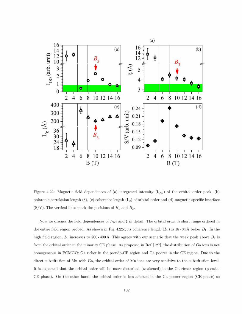
Figure 4.22: Magnetic field dependences of (a) integrated intensity (IOO) of the orbital order peak, (b)
polaronic correlation length (ξ), (c) coherence length (Lc) of orbital order and (d) magnetic specific interface
(S/V). The vertical lines mark the positions of B1 and B2.
Now we discuss the field dependences of IOO and ξ in detail. The orbital order is short range ordered in
the entire field region probed. As shown in Fig. 4.22c, its coherence length (Lc) is 18 - 34 A below B1. In the
high field region, Lc increases to 200 - 400 A. This agrees with our scenario that the weak peak above B1 is
from the orbital order in the minority CE phase. As proposed in Ref. [127], the distribution of Ga ions is not
homogeneous in PCMGO: Ga richer in the pseudo-CE region and Ga poorer in the CE region. Due to the
direct substitution of Mn with Ga, the orbital order of Mn ions are very sensitive to the substitution level.
It is expected that the orbital order will be more disturbed (weakened) in the Ga richer region (pseudo-
CE phase). On the other hand, the orbital order is less affected in the Ga poorer region (CE phase) so
102
that it is more robust and long range ordered. We note that this type of short range orbital order peak
may also be regarded as the signature of the correlations between polarons [56, 57]. Under this scenario,
although the integrated intensity drops to zero when the bulk ferromagnetic order is triggered, it will be
temporarily enhanced in close proximity to the ferromagnetism, as observed in Refs. [56, 57]. For ξ, which
probes the carrier hopping range within one polaron, larger ξ below 6 T may indicate the weaker electron
phonon coupling strength in the pseudo-CE phase. As a result, the carriers are less localized [46, 47]. The
drop of ξ between 4 T and 6 T can be explained as the delocalization of carriers in the pseudo-CE region.
As a result, the corresponding ξ diverges and exceeds the probing region of our SANS measurements. When
B>B1, the collapse of electronic phase separation in the minority CE phase is very smooth (Fig. 4.22a & b).
Due to the presence of the nonmagnetic Ga ions which exist as point defects in PCMGO, ξ is expected to
drop to the ionic size of Ga3+ when the electronic phase separation is completely suppressed.
To conclude this subsection, we have proved that the percolation at B1 is caused by the collapse of elec-
tronic phase separation in the majority pseudo-CE phase, while the transition at B2 revealed by the bulk
magnetization measurements is related to the domain dynamics on micrometre (or even larger) scales. As
stated above, electronic phase separation should populate in the whole sample to the best our knowledge.
This means our observation rules out the filamentary percolation scenario proposed in Ref [121]. In other
words, IOO is not supposed to change a lot across B1 if the corresponding percolation is due to the conduct-
ing filaments formation. For some reason, the spins are ‘locked’ across the conducting paths percolation in
PCMGO. An important message revealed by these observations is that the carrier delocalization (magne-
toresistance) in mixed-valence manganese oxides is essentially driven by the electronic phase separation on
atomic scales rather than the long range spin order.
4.2.6 Discussion
A possible candidate for the spin locking in mixed-valence manganese oxides is the strains. As discussed in
Chapter 4.1.4, the martensitic scenario is commonly used to interpret the field induced magnetic avalanches at
very low temperatures. Besides the carrier delocalization which prevails the double exchange interactions, the
elastic energy is also important to realize the ferromagnetic spin alignment. As a result, additional energy is
required to flip the spins which are ‘locked’ by the strains. The strains in PCMGO can be phenomenologically
characterized by the 6 anisotropic strain parameters using the Stephens formalism (see chapter 4.1.4 & 4.2.2).
The field dependences of these anisotropic strains parameters are plotted in Fig. 4.23. At B2, an obvious
anomaly can be seen in all parameters. Except S400 which has relatively larger errors, other strain param-
103
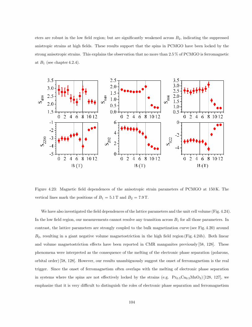
eters are robust in the low field region; but are significantly weakened across B2, indicating the suppressed
anistropic strains at high fields. These results support that the spins in PCMGO have been locked by the
strong anisotropic strains. This explains the observation that no more than 2.5 % of PCMGO is ferromagnetic
at B1 (see chapter 4.2.4).
Figure 4.23: Magnetic field dependences of the anisotropic strain parameters of PCMGO at 150 K. The
vertical lines mark the positions of B1 = 5.1 T and B2 = 7.9 T.
We have also investigated the field dependences of the lattice parameters and the unit cell volume (Fig. 4.24).
In the low field region, our measurements cannot resolve any transition across B1 for all those parameters. In
contrast, the lattice parameters are strongly coupled to the bulk magnetization curve (see Fig. 4.20) around
B2, resulting in a giant negative volume magnetostriction in the high field region (Fig. 4.24b). Both linear
and volume magnetostriction effects have been reported in CMR manganites previously [58, 128]. These
phenomena were interpreted as the consequence of the melting of the electronic phase separation (polarons,
orbital order) [58, 128]. However, our results unambiguously suggest the onset of ferromagnetism is the real
trigger. Since the onset of ferromagnetism often overlaps with the melting of electronic phase separation
in systems where the spins are not effectively locked by the strains (e.g. Pr0.5Ca0.5MnO3) [128, 127], we
emphasize that it is very difficult to distinguish the roles of electronic phase separation and ferromagnetism
104

in the magnetostrictive process of these materials.
Figure 4.24: Magnetic field dependences of (a) the lattice parameters and (b) unit cell volume of PCMGO
at 150 K. The vertical lines mark the positions of B1 and B2.
Electron-phonon coupling (EPC) is very important to the formation of electronic phase separation in CMR
manganites [46, 2, 10, 47]. Besides the ’tolerance factor’ which involves stresses on the Mn-O-Mn bonds from
the ionic size mismatch on the rare-earth (Re) sites (Re1−xAxMnO3), the Jahn-Teller (JT) distortion of the
MnO6-octahedron is another type of EPC [46, 44]. Previous investigations have revealed strong evidence of
the coupling between the JT distortion and the electronic phase separation [55, 131, 160]. For example, the
JT distortion is significantly softened when carrier delocalization occurs [55, 131, 132]. Due to the presence
of the JT distortion, the carriers can be ‘self-trapped’ on atomic scales, causing an insulating state to the
bulk sample [46]. Therefore it is not surprising to observe such softening since a weaker JT state favours
carrier delocalization. However, the JT distortion does not necessarily need to be softened in order to realize
the carrier delocalization from the theoretical point of view [2, 47]. As discussed in Chapter 1.2.6, the JT
distortion can be parameterized by a EPC constant λ. It has been demonstrated by Millis et al that CMR
can be triggered by simply switching on the magnetic field while keeping the value of λ fixed [47].
On the other hand, the JT distortion sometimes leads to orbital order since it breaks the 2-fold degeneracy
of the eg crystal-electric-field (CEF) level [52]. As shown in Fig. 1.6 of Chapter 1.2.6, there are two types of
JT modes which are eg-active. The Q3 mode corresponds a elongation of the Mn-O bond along the b-
105
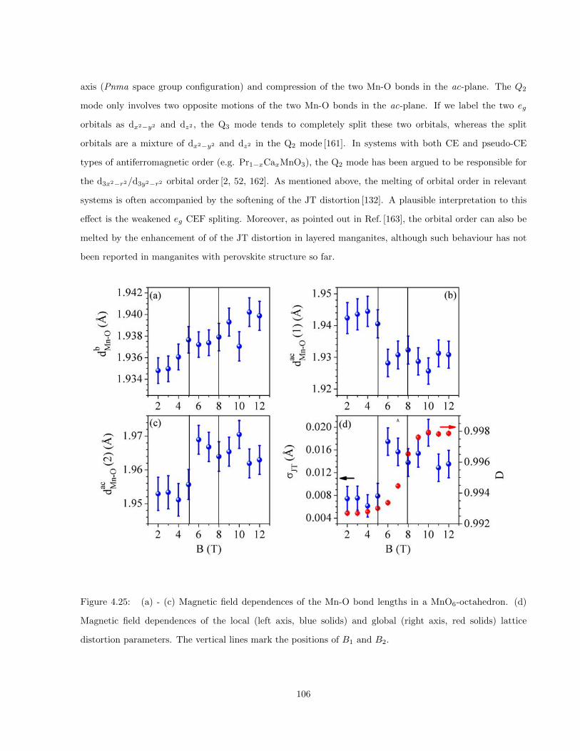
axis (Pnma space group configuration) and compression of the two Mn-O bonds in the ac-plane. The Q2
mode only involves two opposite motions of the two Mn-O bonds in the ac-plane. If we label the two eg
orbitals as dx2−y2 and dz2 , the Q3 mode tends to completely split these two orbitals, whereas the split
orbitals are a mixture of dx2−y2 and dz2 in the Q2 mode [161]. In systems with both CE and pseudo-CE
types of antiferromagnetic order (e.g. Pr1−xCaxMnO3), the Q2 mode has been argued to be responsible for
the d3x2−r2/d3y2−r2 orbital order [2, 52, 162]. As mentioned above, the melting of orbital order in relevant
systems is often accompanied by the softening of the JT distortion [132]. A plausible interpretation to this
effect is the weakened eg CEF spliting. Moreover, as pointed out in Ref. [163], the orbital order can also be
melted by the enhancement of of the JT distortion in layered manganites, although such behaviour has not
been reported in manganites with perovskite structure so far.
Figure 4.25: (a) - (c) Magnetic field dependences of the Mn-O bond lengths in a MnO6-octahedron. (d)
Magnetic field dependences of the local (left axis, blue solids) and global (right axis, red solids) lattice
distortion parameters. The vertical lines mark the positions of B1 and B2.
106
We have explored the field dependences of the Mn-O bonds of PCMGO (Fig. 4.25a-c). When B6B1, the
Mn-O bond along the b-axis (dbMn−O) is shorter than the other two Mn-O bonds in the ac-plane [dacMn−O(1),
dacMn−O(2)]. Since dacMn−O(1) is slightly different from dacMn−O(2), both Q2 and Q3 modes should exist in
this region. When the magnetic field increases from 5 T to 6 T, we cannot resolve any change in the dbMn−O
channel, whereas two opposite motions have been observed in the dacMn−O(1) and dacMn−O(2) channels. This
corresponds to a enhancement of the Q3 mode. This transition can be further addressed by using the JT
distortion constant (σJT )
σJT =
√1
3
∑i=1,2,3
(diMn−O − dMn−O)2, (4.11)
where diMn−O is the individual Mn-O bond length and dMn−O is the mean Mn-O bond length [132]. As
shown in Fig. 4.25d, σJT is clearly enhanced across B1. In contrast, no change can be resolve across B2
in all these parameters. We have also plotted out the global unit cell distortion parameter D =
√b
a+ cin
Fig. 4.25d. Apparently, the unit cell remains robust across B1 and becomes significantly less distorted above
B2, indicating a strong coupling to the spin order.
To finish this subsection, we have proved that the carrier delocalization at B1 is not related to the
filamentary percolation proposed in Ref. [121]. It is caused by the collapse of electronic phase separation
in the whole sample. Contradicting previous experimental investigations [132], the carrier delocalization in
PCMGO is an exceptional case where the JT distortion is enhanced. This is realised by further mixing the
two eg orbitals, dx2−y2 and dz2 , to suppress the d3x2−r2/d3y2−r2 orbital order, rather than recovering the
2-fold degeneracy of the eg level. The spins are ’locked’ in place by the strong anisotropic strains in PCMGO.
While these spins are not coupled to the electronic phase separation, our results unambiguously reveal a
strong spin-lattice coupling on the unit cell level, which is the real cause of the giant magnetostriction effect
commonly observed in these systems.
4.3 Conclusions and future work
In this project, we have investigated the magnetic field dependences of electronic phase separation, spin and
crystallographic structure in the paramagnetic region of the strained manganese perovskite PCMGO. We
have found that the carrier delocalization is caused by the collapse of electronic phase separation in the
whole sample. Surprisingly, this process is assisted by the enhancement of JT distortion (Q2 mode) rather
than the opposite way which has been commonly observed in other perovskite manganites. On the other
hand, the long range ferromagnetic order is insignificant to the carrier delocalization process in this strained
107
compound. We clarify that the giant volume magnetostriction effect does not come from the melting of
electronic phase separation (polarons, orbital order), as proposed in Ref [58, 128]. It is more related to the
strong spin-lattice coupling. Most of all, we emphasize spins are still very important to the magnetoresistance.
As depicted in Fig. 4.19, the R-B curve does not start to flatten until B2. Based on these results,
we propose that the CMR effect is essentially governed by two independent mechanisms: (I)
carrier delocalization caused by the collapse of electronic phase separation (II) ferromagnetic
double-exchange interaction. We stress it is very difficult to distinguish the roles of these two processes
across the magnetoresistive transition in systems where the anisotropic strains are weak.
In the future, it would be very interesting to investigate the magnetic field dependences of electronic phase
separation, spin and crystallographic structure in the magnetic ordered region of PCMGO. Moreover, it is
also worth revisiting the other strained compound Pr0.7Ca0.3MnO3 where bulk ferromagnetism and carrier
delocalization are also separated in the magnetic field [153].
108

CHAPTER 5
DILUTED PYROCHLORE, Y2(CR1−XGAX−0.5SB0.5)2O7
5.1 Background
5.1.1 Magnetic 3d transition-metal pyrochlores
Figure 5.1: (a) Heat capacity versus temperature curves (open squares) of Dy2Ti2O7. The black solids are
the Monte-Carlo simulations for the dipolar-spin-ice model [15]. (b) Illustration of the water ice and spin ice
configurations.
As discussed in Chapter 1.3, the pyrochlore structure has a chemical formula A2B2O7 [15]. Due to the
predominant magnetic dipolar interactions, rare-earth (RE) pyrochlores with nonmagnetic B-sites usually
do not develop long range spin order until very low temperatures, e.g.∼ 1 K in Gd2Ti2O7 [4, 15]. In most
cases, the magnetic ground state is highly degenerate. For example, the ground state spin configuration in
109

RE2Ti2O7 (RE = Dy, Ho) can be described by two spins pointing towards the center of the RE-tetrahedron and
the other two pointing outwards (Fig. 5.1). This two-in/two-out structure is reminiscent of the arrangement
of protons in water ice, so it is named as ‘spin ice’ (Fig. 5.1b). Due to the cubic structure of these pyrochlores
(space group Fd3m), there are six energetically equivalent two-in/two-out spin configurations on each RE-
tetrahedron, and therefore the number of ground states in a bulk sample is infinite, making the system highly
degenerate at low temperatures [15].
Figure 5.2: Heat capacity versus temperature curves of (a) Ho2Mn2O7 and (b) Yb2Mn2O7. The solid lines
are lattice contributions. (c) Field dependences of magnetization of Ho2Mn2O7 and Yb2Mn2O7 collected at
5.0 K. (d) Heat capacity data on Y2Mn2O7 measured by different groups [15].
In sharp contrast, long range ferromagnetic order with very high Curie temperature has been real-
ized in RE pyrochlores with magnetic transition-metal (TM) ions on B-sites (Fig. 5.2a - c) [35]. As shown
in Fig. 5.2a & b, TC is found to be around 38 K in Ho2Mn2O7 and Yb2Mn2O7. Compared with the very low
110

transition temperature (∼ 1 K) in RE pyrochlores with nonmagnetic B-sites, the high TC in RE2TM2O7
indicates the important role of TM ions to the acutual spin ordering.
Although these RE manganese pyrochlores show ferromagnetic behaviour at low temperatures (Fig. 5.2c).
The paramagnetic-to-ferromagnetic order transition window revealed by the heat capacity measurements is
very broad (Fig. 5.2a & b). This may indicate the presence of disorder in those systems. Since these compounds
are not stable at ambient pressure at any temperatures, they must be prepared using high pressure methods
in order to secure the Mn4+ oxidation state [164]. However, a careful check on the valence of the Mn ions
as well as the chemical stoichiometry has not been performed to date. As shown in Fig. 5.2d, heat capacity
data of Y2Mn2O7 reported by different groups show very clear discrepancies [15]. These observations suggest
that the magnetic properties in manganese pyrochlores are very sensitive to the disorder. We also note that
an additional Lorentzian-squared term is required to produce satisfactory fits to the small angle neutron
scattering data collected in these system [35]. This Lorentzian-squared term is commonly found in materials
with site-disorder.
5.1.2 Structural disorder and magnetism
The disorder in manganese pyrochlores is related to the quality of the samples. It has been suggested
that structural disorder could well be intrinsic in other pyrochlore compounds, and more importantly, be
responsible for the lack of long range spin order in corresponding systems [15, 24, 25, 26, 29, 30, 165, 166,
167]. For example, a dipolar spin ice model, which contains the nearest neighbour exchange and long range
dipolar interactions [168], has been argued to be appropriate to describe Tb2Ti2O7. Using the estimated
values of the coupling constants, a long range antiferromagnetic order should develop below ∼ 1 K. However,
neutron scattering measurements on both single crystals and powder of Tb2Ti2O7 have revealed no static
magnetic order but short range correlations between Tb3+ spins on the nearest neighbour scales down to 50
mK [169, 170]. Moreover, muon spin relaxation measurements have only observed paramagnetic fluctuations
down to 60 mK [171]. As a result, the magnetic ground state of Tb2Ti2O7 has been established to be a spin
liquid (or cooperative paramagnet) [15]. On the other hand, the crystal field degeneracy of the non-Kramer
Tb3+ ion is susceptible to Jahn-Teller distortions [172]. Since the magnetoelastic coupling usually suppresses
frustration [173, 174], the spin liquid state of Tb2Ti2O7 may suggest frustration in lattice degrees of freedom
as well [175]. In other words, intrinsic lattice disorder plays a key role in the spin liquid physics of Tb2Ti2O7
through the magnetoelastic coupling, as revealed by multiple experiments [165, 166, 167].
111

Figure 5.3: PDF as a function of distance r of Y2Mo2O7 at various temperatures. The fits are based on a
fully ordered model with anisotropic atomic displacement factors for all atoms [25]
As discussed in Chapter 1.3.2, the spin glass state in Y2Mo2O7 has been ascribed to the local structure
disorder. It is also demonstrated in Ref. [25] that the fits to the neutron pair-distribution-function (PDF)
always become worse on cooling, indicating the development of local disorder (Fig. 5.3). However, this
does not necessarily suggest any magnetoelastic coupling, as has been revealed in the Tb2Ti2O7, due to
the presence of disorder in both local and average structures at 300 K (Fig. 5.3). Recently, a new model,
in which the four Mo4+ ions on each Mo-tetrahedron obey a two-in/two-out displacement rule, has been
proposed by Thygesen et al based on their analyses of both X-ray and neutron PDF data [32]. They have
highlighted the key role of orbital frustration. The disorder of the spin exchange interaction comes from
the resulting cooperative O2− ion displacements. Nonetheless, the bond disorder level in Y2Mo2O7 is too
weak to generate any spin glass state according to the conventional mean field theory predictions [27]. This
112

puzzle has been solved by Saunders et al who have successfully introduced a spin glass state at the weak
bond disorder limit [29]. However, the spin freezing temperature (T f) would scale with the disorder strength
(∆) in this model. This leads to an estimated T f which is 20-30 times smaller than that determined by the
experiments [30]. In order to fully reproduce the spin glass transition as well as the high T f in Y2Mo2O7,
the spin-lattice coupling term is required (Fig. 5.4), as demonstrated by Ref. [30].
Figure 5.4: Bond disorder strength (∆) - temperature (T) phase diagram obtained at b = 0.2, where b is
the spin-lattice coupling constant [30]. The nematic and spin glass transition temperatures are denoted by
squares and circles.
113

5.1.3 RE2(Cr0.5Sb0.5)2O7, RE = Ho, Y, Dy, Tb, Er, etc
Figure 5.5: Neutron powder diffraction patterns (λ= 1.8857A) of Ho2(Cr0.5Sb0.5)2O7 at (a) 298 K and (b)
1.5 K. Inset of (b): The refined magnetic structure at 1.5 K.
114
Nonmagnetic ion dilution in pyrochlores can be traced back to 1960s, when Bongers et al investigated the bulk
magnetism of RE2(Cr0.5Sb0.5)2O7 (RE = Ho, Y, Dy, Tb, Er, etc) [176]. For the Ho2(Cr0.5Sb0.5)2O7 compound,
it enters into a ferromagnetic-like state below TC ∼ 10 K [176]. This value is considerably larger when the
B-site is completely nonmagnetic (∼ 1 K in Ho2Ti2O7), indicating the important role of the magnetic TM ions
on B-site. Neutron powder diffraction experiments have been carried out on Ho2(Cr0.5Sb0.5)2O7 by Whitaker
et al [177]. Sharp magnetic reflections are clearly observed at low temperatures (Fig. 5.5). By assuming the
four Ho3+ spins on each tetraheron obey the two-in/two-out configuration and Cr3+ spins ferromagnetically
align along the c-axis [Fig. 5.5b(inset)], they have successfully refined the diffraction pattern at 1.5 K. Unlike
the highly frustrated two-in/two-out spin ice state in Ho2Ti2O7 [15], Whitaker et al have also suggested the
two-in/two-out structure of Ho3+ spins in Ho2(Cr0.5Sb0.5)2O7 is actually ordered due to the presence of
Ho3+-Cr3+ coupling [177].
5.2 Results
5.2.1 Research motivations
As reported in Ref. [177], Ho2(Cr0.5Sb0.5)2O7 develops long range magnetic order below 13 K. Ho3+-Cr3+
coupling plays a key role on the ordering of Ho3+ ions. However, it is not clear how this Ho3+-Cr3+ coupling
will affect the Cr3+ ordering. According to Bongers et al, the effective Cr3+-Cr3+ spin exchange is ferromag-
netic with Curie-Weiss temperature θCW ∼ 15 K [176]. At the first sight, one would expect an ordered (or
partially ordered) magnetic ground state in Y2(Cr0.5Sb0.5)2O7 since the Sb fraction (0.5) is still well below
the nonmagnetic ion percolation threshold on a pyrochlore lattice xc = 0.61 [178]. Moreover, Cr3+ is stable at
ambient pressure. This means the valence disorder which hinders the long range magnetic order in Y2Mn2O7
should not be important in Y2(Cr0.5Sb0.5)2O7.
It has been theoretically proposed that very weak bond disorder can introduce a spin glass state [29, 30].
In this model, the spin freezing temperature T f does not depend on the disorder level ∆ if there is spin-lattice
coupling in the system [30], as experimentally verified in Y2Mo2O7 [23]. However, T f will scale with ∆ in
the absence of spin-lattice coupling, and therefore be significantly lowered at the weak bond disorder limit
(Fig. 5.4) [29, 30]. As pointed out recently, the spin-lattice coupling in Y2Mo2O7 is essentially mediated by the
orbital degrees of freedom [32]. In magnetic 3d TM pyrochlores, the orbital moment is usually quenched [4],
which indicates the spin-lattice coupling is probably not dominant in these systems. As a result, the TM
pyrochlore family with very weak bond disorder is an ideal candidate to test the spin glass theory proposed
115

in Ref. [29, 30] at zero spin-lattice coupling limit.
The spinel compound ZnCr2O4, in which the Cr3+ ions form a pyrochlore sublattice with corner-sharing
tetrahedra, is also worth mentioning. It enters into a co-planar antiferromagnetic state below TN = 12.5 K [179].
Since the cubic pyrochlore lattice with Heisenberg-type antiferromagnetic interactions cannot order [15], the
onset of antiferromagnetism has been attributed to the spin-driven lattice symmetry breaking at TN [179, 180,
174, 181]. As a result, a cooperative spin-lattice coupling exists in this special case, as included in the spin-
glass model by Shinaoka et al to account for the spin freezing transition in Zn1−xCdxCr2O4 (x> 0.01) [182].
More importantly, we highlight the magnetic ground state switches from antiferromagnetic to spin glass by
nonmagnetic ion dilution in Zn(Cr1−xGax)2O4 when x is between 0.2 and 0.25 [183, 184]. This critical value
is much lower than the nonmagnetic ion percolation threshold on a pyrochlore lattice: xc = 0.61 [178]. Non-
magnetic ion dilution can cause random distortion to the spin exchange network formed by TMO6-octahedra
due to the size mismatch between nonmagnetic and magnetic ions, and therefore leads to bond disorder. The
ionic radii of Ga3+ and Cr3+ are 0.62 A and 0.615 A, respectively. This places Zn(Cr1−xGax)2O4 to the weak
bond disorder limit. However, T f is not sensitive to ∆ in this compound due to the presence of spin-lattice
coupling [30].
Based on the discussions above, we have demonstrated that bond disorder is essential to understand the
spin glass state on a pyrochlore lattice. The spin freezing temperature T f is controlled by the bond disorder
strength ∆ and spin-lattice coupling. While the theories proposed by Saunders et al [29] and Shinaoka et
al [30] have been tested in the presence of both spin-lattice coupling and weak bond disorder, they have not
been verified in systems without spin-lattice coupling yet. In the following, we have proposed a potential TM
pyrochlore candidate Y2(Cr0.5Sb0.5)2O7 to test the relevant theories.
5.2.2 Data analysis
The neutron powder patterns have been refined using the Rietveld method described in Appendix A. We have
adopted the general crystallographic structure for a pyrochlore with space group Fd3m in our refinement [15].
The lattice parameters, atomic positions and isotropic atomic displacement parameters (Biso) in Ref. [177] by
refining the room temperature X-ray diffraction pattern of Y2(Cr0.5Sb0.5)2O7 have been used as the starting
parameters in our refinements. A Thompson-Cox-Hastings pseudo-Voigt convoluted with axial divergence
asymmetry function has been used to fit the peak shape of the nuclear reflections [106]. The magnetic Bragg
peaks which can be observed at high magnetic fields were fitted by a Gaussian function [106].
116

5.2.3 Absence of magnetic order in Y2(Cr0.5Sb0.5)2O7: a spin glass candidate
Introduction
Magnetic frustration refers to systems where the total free energy cannot be minimized by optimizing the
interaction energy between each pair of spins [1]. It is responsible for the abundant spin structures in py-
rochlore compounds where ‘geometric frustration’, i.e. corner-sharing tetrahedral network consisting of mag-
netic cations, coexist with competing spin interactions [15]. The consequential magnetic ground state can
be highly degenerate (spin liquid) in a Heisenberg magnet with antiferromagnetic spin exchange interac-
tions [185, 186]. This degeneracy can be partially lifted in rare-earth compounds R2Ti2O7 (R = Dy, Ho) to
form a exotic state called ‘spin ice’ [15, 187, 188]. Strikingly, the quasiparticles excitations of a spin ice state
are found to resemble the behaviour of magnetic monopoles [189, 190]. Moreover, peculiar long range order
can also result in relevant systems. The low temperature spin modulation in Gd2Ti2O7 was initially proposed
to be 4-k with propagation vector k = [ 121212 ]∗ [113]. Recently, this solution has been theoretically reproduced
by taking into account the thermal fluctuations which were not accessible within mean-field approaches [114],
but this model was challenged by Paddison et al recently [191]. Strong evidence using neutron diffraction
measurements has been provided to show it is essentially 1-k modulation in Gd2Ti2O7 [191].
Another interesting state which may rise in pyrochlores is spin glass (SG). In general, a SG state prevails
in systems dominated by randomness and frustration. For example, the sign of Ruderman-Kittel-Kasuya-
Yosida (RKKY) interaction in lightly doped Au1−xFex (x∼ 0.05) is very sensitive to the distance between
Fe-sites [192, 193]. SG in this class of materials is induced by zero-point spin exchange fluctuations, i.e
competing antiferromagnetic and ferromagnetic spin interactions. SG is also commonly observed in diluted
magnets around the nonmagnetic site percolation threshold [194]. Compared with these classic systems, the
appearance of SG on a ’clean’ pyrochlore lattice is nontrivial to understand. Clear signatures of SG have
been observed in Y2Mo2O7 [23, 195, 21]. Recent advancement in theory strongly point to the key role of
weak bond disorder on the spin freezing in geometically frustrated antiferromagnets [29, 196]. Moreover, an
additional spin-lattice coupling term is required to correctly reproduce the spin freezing temperature (Tf )
of Y2Mo2O7 [30]. These theories can also be applied to other SG compounds such as Zn1−xCdxCr2O4 and
Zn(Cr1−xGax)2O4 [30, 182, 183, 184]. On the other hand, Tf is expected to be controlled by the disorder
strength (∆) in the absence of spin-lattice coupling [29]. This will significantly reduce the onset temperature
of SG in relevant systems [30]. In Mo-pyrochlores, the spin-lattice coupling is essentially mediated by the
orbital degrees of freedom [32, 197]. However, this contribution is often insignificant in 3d transition-metal
(TM) pyrochlores due to the orbital quenching effect, making them ideal systems to validate the theory in
117

the zero spin-lattice coupling limit. We note the cooperative spin-lattice coupling in the other 3d TM family,
Zn1−xCdxCr2O4 and Zn(Cr1−xGax)2O4, is related to a novel spin-Peierls-like phase transition, rather than
the conventional orbital physics [179, 180, 174, 181].
Following this idea, we have synthesized Y2(Cr1−xGax−0.5Sb0.5)2O7 (0.56 x 6 0.9) for investigation. By
randomly substituting the magnetic TM ions (Cr) with nonmagnetic ions (Sb/Ga), we have created site
disorder which is a conventional way of approaching SG [194]. Most of all, bond disorder is also introduced into
our samples due to the size mismatch between magnetic and nonmagnetic ions. This feature has been proven
to be responsible for the SG state in geometrically frustrated magnets. For the Y2CrSbO7 (x = 0.5) sample
which is well below the nonmagnetic site percolation threshold (xc' 0.61) [178], our high-resolution neutron
powder diffraction (HRNPD) measurements cannot detect any long range spin order down to 2 K. This is in
sharp contrast with the prevailing ferromagnetic spin exchange interactions as revealed by θCW = 20.1(6) K.
Compared with nonmagnetic site percolation, our simulations concerning disordered bond percolation predicts
a much lower threshold (x′c' 0.23). x′c is in excellent agreement with the onset of SG in Zn(Cr1−xGax)2O4
where x is between 0.2 and 0.25 [183, 184]. Our Rietveld refinement confirms the average Cr-O-Cr bond
angle [130.19(2)] is in the critical region where the corresponding spin exchange constant changes its sign.
The resulting zero-point spin exchange fluctuations may further assist the formation of SG in Y2CrSbO7
(x = 0.5).
Experiments
Polycrystalline samples of Y2(Cr1−xGax−0.5Sb0.5)2O7 (0.5 6 x 6 0.9) were synthesized by the traditional solid
reaction method. A homogeneously ground mixture of GaSbO4 (CrSbO4) and Y2O3 (4N) were heated in air
for 6 days at 1200 C with several intermediate regrindings to prepare Y2GaSbO7 (Y2CrSbO7). GaSbO4
(CrSbO4) raw materials were preprared by sintering Ga2O3 (Cr2O3) (3N) and Sb2O3 (3N, 5 % excess to
compensate the volatilization) for 3 days at 640 C, and then 5 days at 1200 C with several intermedi-
ate regrindings as well. The intermediate temperature (640 C) is to transform Sb2O3 into Sb2O4. Finally,
Y2Cr1−xGaxSbO7 were obtained by heating the stoichiometrically mixed Y2GaSbO7 and Y2CrSbO7 powders
for 5 days at 1200 C.
The room temperature crystallographic structure of each sample was checked by the X-ray powder diffrac-
tion technique using a Bruker D8 diffractometer (Cu Kα1,λ= 1.5406 A). Magnetic susceptibility data were
collected using a Magnetic Property Measurement System (MPMS, Quantum Design).
118

Figure 5.6: (a) χ-T (left axis) and 1/χ-T (right axis) curves of Y2CrSbO7 measured at B = 0.01 T. The black
solid curve is a Curie-Weiss fit to the linear part of the χ-T curve at high temperatures. (b) Nonmagnetic
ion substitution level (n) dependence of site percolation probability (p). (c) Fraction of percolative magnetic
clusters (fm) as a function of the nonmagnetic ion fraction (n). The results were obtained by a 50-times
sampling simulation on a N×N×N (N = 64) lattice.
119

HRNPD patterns were collected at the D2B powder diffractometer (λ= 1.594 A) equipped with a 5-
Tesla vertical cryomagnet at the Institute Laue-Langevin (ILL) in Grenoble, France. About 8 g of powder
was hydraulically pressed into a cylinder (height = 11 mm, diameter = 13 mm) to avoid any field-induced
texture and then loaded into a vanadium container. Rietveld refinements were performed using the FullProf
package [102, 106].
A minor impurity phase YCrO3, with volume fraction 3.4(2) %, is necessary to match some very weak
peaks in our HRNPD patterns [Fig. 5.7(inset)]. The onset of antiferromagnetism in YCrO3 is responsible for
the kink around 142 K in our susceptibility curves (data not shown here) [177]. As a result, we will only show
susceptibility data measured below 120 K in the following.
Main results and discussion
Figure 5.7: (main panel) HRNPD pattern (red solids) of Y2CrSbO7 at T = 2.0 K, B = 0 T. Calculated pattern
(black line), nuclear Bragg positions (blue vertical line) and difference (purple line) are also displayed. (inset)
Enlarged version of a selected angle region. Additional peaks from YCrO3 (red arrows) and V (black arrow)
can be visualized.
120

The low field (B = 0.01 T) susceptibility (χ) data of Y2CrSbO7 is shown in Fig. 5.6a. Although distinct
deviation from standard paramagnetic behaviour sets in below ∼ 40 K, no magnetic transition can be observed
down to the lowest temperature probed (1.8 K). By fitting the linear part of the inverse susceptibility (1/χ)
versus temperature curve between 40 K and 120 K, we obtained TCW = 20.1(6) K, meaning Y2CrSbO7 is a
highly frusrated system dominated by ferromagnetic spin exchange interactions. This is in sharp contrast
with the fully occupied compound Y2Mn2O7 (same electronic configuration 3d3) which has a ferromagnetic-
like state below 15 K [33, 34]. The absence of ferromagnetism in Y2CrSbO7 is confirmed by the HRNPD
pattern measured at 2.0 K (Fig. 5.7). Only nuclear reflections can be resolved in our refinement. The refined
crystallographic parameters of Y2CrSbO7 (x = 0.5) and Y2Cr0.4Ga0.6SbO7 (n = 0.8) at 2.0 K are listed in
Table 5.1.
Table 5.1: Structural parameters of Y2CrSbO7 and Y2Cr0.4Ga0.6SbO7. The corresponding HRNPD patterns
were refined under space group Fd3m (a = b = c, α= β= γ= 90). The only atomic position needs to be
refined is O2 (x, 0.125, 0.125) [177].
Y2CrSbO7 Y2CrSbO7 Y2CrSbO7 Y2Cr0.4Ga0.6SbO7
T = 300 K, B = 0 T T = 2 K, B = 0 T T = 2 K, B = 5 T T = 2 K, B = 0 T
a (A) 10.1620(1) 10.15235(7) 10.15143(5) 10.15081(8)
x (O2) 0.4178(1) 0.41793(8) 0.41792(9) 0.4182(1)
B iso (Y) (A2) 0.72(2) 0.69(1) 0.65(1) 0.58(1)
B iso (Cr) (A2) 0.44(2) 0.34(1) 0.31(1) 0.51(2)
B iso (O1) (A2) 0.15(3) 0.17(2) 0.08(2) 0.17(3)
B iso (O2) (A2) 0.45(1) 0.439(8) 0.399(9) 0.37(1)
Cr - O2 (A) 1.9810(6) 1.9787(3) 1.9785(4) 1.9774(5)
Cr - Cr (A) 3.59282(3) 3.58940(2) 3.58907(1) 3.58885(2)
Cr - O2 - Cr () 130.14(2) 130.19(1) 130.19(2) 130.31(2)
As mentioned above, a SG state often emerges in systems close to the nonmagnetic site percolation
threshold. To check the influence of site disorder in Y2CrSbO7, we have simulated the fraction of percolative
magnetic ions (fm) as well as percolation probability (p) at various nonmagnetic ion substitution levels
(x ). Our model predicts a site percolation threshold xc' 0.61 which is consistent with previous studies
(Fig. 5.6b) [178]. More importantly, 83 % of the sample (x = 0.5) is populated by the percolative magnetic
sites as shown in Fig. 5.6c. This suggests that site disorder is not strong enough to affect the magnetic
121

properties of Y2CrSbO7 yet.
Figure 5.8: (a) Magnetization (M) - temperature (T) curve (purple) of Y2CrSbO7 at 5 T. The black solids is
the derivative of the M-T curve. The red arrow marks the position of TC. (b) TC - x plot (pink). xc is
labeled by the red line.
122

Figure 5.9: (a) Magnetization (M) versus magnetic field (T) curve (red solids) of Y2CrSbO7 at 2 K. The blue
line is a linear fit to the data above 3.5 T. (b) HRNPD pattern and the Rietveld refinement of Y2CrSbO7 at
2 K/5 T. The blue arrow marks the ferromagnetic reflection at the reciprocal position (1, 1, 1).
123

f m is very sensitive to x in the critical region of nonmagnetic site percolation (Fig. 5.6c). Thus another
possible explanation for the absence of magnetic order in the synthesized Y2CrSbO7 is off-stoichiometry
towards the x > 0.5 side. In order to rule out this scenario, we have studied the temperature dependence
of magnetization in Y2(Cr1−xGax−0.5Sb0.5)2O7 (0.5 6 x 6 0.9) in the high field region where the magnetic
frustration is suppressed. As shown in Fig. 5.8a, ferromagnetic-like behaviour is recovered under B = 5 T evi-
denced by a weak plateau at low temperatures. The Curie temperature (TC) is determined by the minimum
in the corresponding derivative curve. TC as a function of x is displayed in Fig. 5.8b. A sudden decrease of
TC is observed between x = 0.6 and x = 0.8. This is consistent with the nonmagnetic site percolation at
x c' 0.61 (Fig. 5.6b). Moreover, the magnetization (M ) of Y2CrSbO7 shows linear dependence on magnetic
field above B = 3.5 T (Fig. 5.9a). Extrapolating the high field M-B curve produces a saturation moment
(Msat) around 2.585µB/Cr. On the other hand, the total magnetic moment (Mtot = gJ, where g is the Lande
g-factor and J is the total angular momentum) of the Cr3+ ion can be obtained by fitting the linear part of the
low field 1/χ-T curve in Fig. 5.6a. By assuming the g is 2, we get Mtot = 3.12µB/Cr. The difference between
Msat and Mtot can be explained by the presence of non-percolative spin clusters in Y2CrSbO7 (Fig. 5.6c). As
a result, f m is around 83 % in Y2CrSbO7. This generates an effective nonmagnetic ion fraction xeff exactly
around 0.5. This confirms off-stoichiometry is not present in Y2CrSbO7. We have also refined the magnetic
structure at B = 5 T (Fig. 5.9b). This corresponds to a simple collinear ferromagnetic alignment along the
c-axis with a propagation vector k = (0, 0, 0) and an effective moment 2.4(1)µB/Cr. We note the spins can
also point along are axes due to the cubic symmetry (Fd3m) of a pyrochlore structure.
Besides the site disorder induced by random nonmagnetic ion substitution, bond disorder also exists in
such systems due to the inevitable size mismatch between magnetic and nonmagnetic ions. The ionic radii
of Cr3+, Sb5+ and Ga3+ are 0.615 A, 0.60 A and 0.62 A, respectively. The small variations of ionic radii on
B-site puts Y2CrSbO7 to the weak bond disorder limit. The effect of nonmagnetic ion substitution can be
readily demonstrated by the x -dependences of Cr-O2-Cr bond angle, the Cr-O2 bond length and the isotropic
atomic displancement parameter of O2 in Table 5.1. Due to the random substitution of B-sites with Sb5+
ions, there are five Cr/Sb-tetrahedral configurations randomly distributed in the sample, corresponding to
empty, single, double, triple and full occupation by Cr ions (Fig. 5.10a - e). The bond disorder could apply
random strains to the BO6-octahedron, leading to random deviations of the Cr-O2-Cr bond angle from the
average value (Fig. 5.10f). We have calculated the substituting region where percolative magnetic clusters
exclusively consisting of fully Cr-occupied tetrahedral can be found (Fig. 5.10a). In this case, there will be no
bond disorder in the corresponding percolative magnetic region. As shown in Fig. 5.11a, the new percolation
124

threshold (x ′c' 0.23) is signicantly reduced compared with x c' 0.61 for site disorder. Most of all, this model
is consistent with the observations in Zn(Cr1−xGax)2O4 where the Cr/Ga sublattice also has a pyrochlore
structure [183, 184]. While ZnCr2O4 has a antiferromagnetic ground state, substitution Cr3+ with Ga3+
switches this system to SG between x = 0.2 and x = 0.25 [183, 184]. Moreover, the effective ordered moment
is reduced by a factor of 20 % even at x = 0.05, which is close to 26 % predicted by our model. As a result,
our model should capture the essential physics in Y2CrSbO7. Y2CrSbO7 (x = 0.5) is in a region dominated
by bond disorder. We also note the fast drop of f m even below x ′c (Fig. 5.11b). This indicates the fraction
of long range order in relevant systems is extremely sensitive to the bond disorder strength even at the weak
limit.
Figure 5.10: (a) - (e) Five possible configurations of a single Cr/Sb-tetrahedron. The bonds are displayed by
dual-band cylinders. (f) Possible influence of bond disorder to the local structure in a unit cell. O2 oxygens
(green spheres) will deviate from their average position (translucent green spheres), producing a random
distribution of Cr/Sb-O2-Cr/Sb bond angles in the sample (red dotted lines). The Cr/Sb-tetrahedral network
is linked by black lines.
125
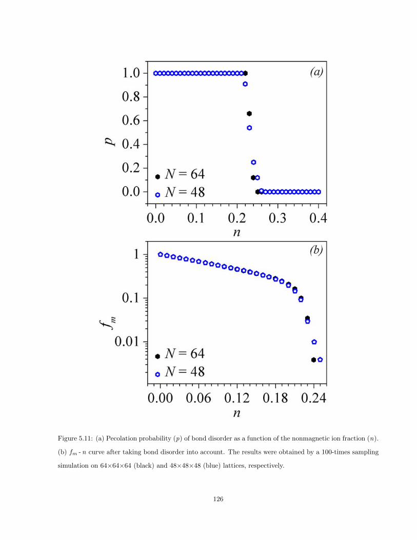
Figure 5.11: (a) Pecolation probability (p) of bond disorder as a function of the nonmagnetic ion fraction (n).
(b) fm - n curve after taking bond disorder into account. The results were obtained by a 100-times sampling
simulation on 64×64×64 (black) and 48×48×48 (blue) lattices, respectively.
126

Based on the prevailing bond disorder and the lack of long range order down to 1.8 K of Y2CrSbO7,
we propose SG as its possible magnetic ground state. The SG in Y2CrSbO7 may be further assisted by
the zero-point spin exchange fluctuations. The refined average Cr/Sb-O2-Cr/Sb bond angle and Cr/Sb-O2
distance are 130.19(1) and 1.9783(3) A, respectively (Table 5.1). According to the Goodenough-Kanamori
rules [12, 198], the nature of TM-O-TM spin exchange is mostly determined by the exchange bond angle and
the bond lengths. While both bond distance and the type of ion are fixed, the bond angle becomes the only
dominant parameter. Y2CrSbO7 belongs to a series of Cr3+ oxides with almost identical values of Cr-O bond
length [199]. As investigated in Ref [199], 130.19(1) is in a critical region where the effective spin exchange
constant changes its sign. The zero-point spin fluctuations could be triggered by the bond disorder, as shown
in Fig. 5.10f.
The appearance of such SG states in weakly disordered pyrochlore lattices has been studied, e.g. Y2Mo2O7 [29,
196, 30]. It is shown that a SG can appear at very low bond disorder level. The corresponding T f will be
very low (scale with ∆) unless the spin-lattice coupling term is included. For Y2CrSbO7, the spin-lattice
coupling effect is expected to be insignificant due to the orbital quenching effect. On the other hand, the
disorder strengh is also weak evidenced by the small ionic size mismatch on B-sites. This makes Y2CrSbO7
a candidate to study purely weak bond disorder induced SG state in the absence of spin-lattice coupling.
5.3 Conclusions and future work
In summary, we have carried out susceptibility and HRNPD measurements on Y2(Cr1−xGax−0.5Sb0.5)2O7
(0.56 x 6 0.9). While Y2CrSbO7 is not sensitive to nonmagnetic site disorder based on multiple evidence,
we cannot observe any long range order down to the lowest temperature probed (1.8 K). We propose the
bond disorder caused by the ionic size mismatch between Cr3+ and Sb5+ is the origin of this phenemenon.
Further assisted by the zero-point spin exchange fluctuations, Y2CrSbO7 may be another SG candidate
among pyrochlores. Unlike Y2Mo2O7, the SG state in Y2CrSbO7 is exclusively caused by weak disorder
effect.
Our results also provide important motivations to future studies. For example, lower temperature
(T < 1.8 K) characterizations are neccesary to confirm the real state of Y2CrSbO7 above T = 0 K. More-
over, new materials are demanded to test n ′c predicted by our geometry model.
127
CHAPTER 6
SUMMARY
6.1 γ-CoV2O6
We have performed neutron diffraction studies on the quasi-one-dimensional magnet γ-CoV2O6, which pos-
sesses competing magnetic interactions but not geometric frustration. We have found that the low tem-
perature magnetic reflections can be indexed by two propagation vectors, k1 = (0.5, 0, 0) and k2 = (-
0.25, 0, 0.25). More importantly, we propose that this compound develops two single-k phases in a volume
ratio of 65(1) : 35(1) below TN = 6.6 K. By further decreasing the temperature, the minority phase modulated
by k2 undergoes an incommesurate-commensurate lock-in transition at T ∗ = 5.6 K.
6.2 Pr0.5Ca0.5Mn0.97Ga0.03O3
We have studied the strained manganese perovskite Pr0.5Ca0.5Mn0.97Ga0.03O3 (PCMGO). By varying the
magnetic field at T = 150 K, where PCMGO has a paramagnetic ground state, the carrier delocalization
driven by the collapse of electronic phase separation (orbital order, polarons) occurs at Bc1 = 5.1 T. Surpris-
ingly, the Jahn-Teller distortion is enhanced above Bc1, contradicting the softening picture reported previ-
ously. On the other hand, the spins remain mostly paramagnetic across Bc1 and do not become ferromagnetic
at a much higher field Bc2 = 7.9 T, where a giant magnetostriction effect is observed. This decoupling between
carrier delocalization and ferromagnetism is related to the prevailing anisotropic strains in PCMGO. Most
of all, the magnetoresistance in PCMGO can be detected up to Bc2, rather than Bc1. These results strongly
suggest that colossal magnetoresistance is driven by two independent forces: (I) carrier delocalization, and
(II) ferromagnetic double-exchange.
128
6.3 Y2(Cr1−xGax−0.5Sb0.5)2O7, 0.56 x 6 0.9
We have studied the magnetism of the diluted transition metal pyrochlores Y2(Cr1−xGax−0.5Sb0.5)2O7
(0.56 x 6 0.9). Although Y2CrSbO7 (x = 0.5) is well below the nonmagnetic site percolation threshold
xc' 0.61, both susceptibility and neutron powder diffraction measurements cannot detect any magnetic
long range order down to 2 K. We propose that the magnetic long range order in Y2CrSbO7 is suppressed
by the bond disorder, which has a much lower percolation threshold x′c' 0.23 based on our simulations,
caused by the weak ionic size mismatch between Cr3+ and Sb5+. Bond disorder in pyrochlores can lead to a
spin glass at low temperatures. In the absence of spin-lattice coupling, the spin freezing temperature scales
with the bond disorder strength based on the recent spin glass theories [30, 29]. As a result, Y2CrSbO7 is a
potential spin glass candidate with a very low spin freezing temperature due to its very weak bond disorder
and zero spin-lattice coupling.
129

APPENDIX A
RIETVELD REFINEMENT
Experimentally, the ith intensity (I obs, i), together with the corresponding standard deviations (σi), of a
diffraction pattern is always recorded as a function of some variable (xi), e.g. scattering angle, time-of-flight
or energy. On the other hand, the calculated profile I calc can be expressed as
Icalc, i =∑n
Sn∑Q
In,QΩ(xi − xn,Q) + bn, (A.1)
where n labels the phase number, Sn is the scale factor, Q labels the Bragg reflection position, In,Q is the
calculated intensity, Ω is the reflection profile function which models both instrumental and sample effects,
bn is the background. Some of these parameters, e.g. L ad F have already been discussed in Chapter. 2.2.
In FullProf, the general expression of In,Q can be writen as
In,Q =L, A, P, C, F 2
n,Q
, (A.2)
where L contains the Lorentz, polarization and mutiplicity factors, F is structure factor, A is the absorption
correction, P is the preferred orientation function and C includes the spherical corrections [102]. In the
Rietveld refinement process, I calc is being optimised by minimizing the chi-square parameter
χ2 =∑i
wi
Iobs, i − Icalc, i(α)
2
, (A.3)
where wi is the weigting factor, α=α1,α2,α3...
stands for the parameter space to be determined. From
mathematical point of view,
∂χ2
∂α
αopt
= 0 once the optimum parameters are (αopt) found [106].
By providing some initial guessing paramters αini, a Taylor expansion can be applied to I calc(α) around
I

αini to start the iterative process. Until a convergence criterion is satisfied, the shifts of the parameters δα
by solving the normal equations in the mth cycle will be added to the starting parameters of the (m + 1)th
cycle: (αini)m+1 = (αini)m + δα,m. After finishing the simulation, an individual set of parameters are used
to judge the quality of this refinement. They include the profile factor Rp, the weighted profile factor Rwp
which can be expressed by [106]
Rp = 100 ×∑i |Iobs, i − Icalc, i|∑
i Iobs, i, (A.4)
Rwp = 100 ×∑
i wi|Iobs, i − Icalc, i|2
wi∑i I
2obs, i
1/2
. (A.5)
In practice, a Rieveld refinement can easily get stuck due to various reasons such as a bad choice of starting
parameters, correlation between paramters and the large number of paramters to be fitted. As a result, some
expertise are required. For example, background, zero shift of the detector and lattice parameters can be
obtained first by an alternative Lebail profile matching approach [148]. Moreover, it is sensible to refine the
parameters step-by-step in the early stage. Although the detailed refinement procedure is sample specific, a
recommended sequence is summarized below [102]:
1, Scale factor.
2, The sloppy part of the background.
3, Atomic positions and Debye-Wallter factors.
4, Peak shape function and asymmetry parameters.
5, Microstructural parameters if required.
...
II

LIST OF REFERENCES
[1] H. T. Diep. Frustrated Spin Systems. World Scientific, 2nd edition, 2013.
[2] Elbio Dagotto. Nanoscale Phase Separation and Colossal Magnetoresistance. Springer, 2003.
[3] https://www.khanacademy.org/science/chemistry/electronic-structure-of-atoms/
orbitals-and-electrons/a/the-quantum-mechanical-model-of-the-atom.
[4] Stephen Blundell. Magnetism in Condensed Matter. Oxford University Press, 2011.
[5] I. M. Rae, Alastair. Quantum Mechanics. Adam Hilger, 2nd edition, 1986.
[6] P. A. M. Dirac. The principles of quantum mechanics. Oxford University Press, 4th edition, 1958.
[7] M. Gerloch and R. C. Slade. Ligand-Field Parameters. Cambridge University Press, 1973.
[8] Zu-Fei Huang, Fei Du, Chun-Zhong Wang, Deng-Pan Wang, and Gang Chen. Low-spin Mn3+ ion inrhombohedral LiMnO2 predicted by first-principles calculations. Phys. Rev. B, 75:054411, Feb 2007.
[9] N. Hollmann, S. Agrestini, Z. Hu, Z. He, M. Schmidt, C.-Y. Kuo, M. Rotter, A. A. Nugroho, V. Sessi,A. Tanaka, N. B. Brookes, and L. H. Tjeng. Spectroscopic evidence for exceptionally high orbitalmoment induced by local distortions in α-CoV2O6. Phys. Rev. B, 89:201101, May 2014.
[10] Elbio Dagotto, Takashi Hotta, and Adriana Moreo. Colossal magnetoresistant materials: the key roleof phase separation. Physics Reports, 344(13):1 – 153, 2001.
[11] Gregory H. Wannier. The structure of electronic excitation levels in insulating crystals. Phys. Rev.,52:191–197, Aug 1937.
[12] John B. Goodenough. Magnetism And The Chemical Bond. Wiley, 1963.
[13] Joaqun Garca and Gloria Subas. The verwey transitiona new perspective. Journal of Physics: Con-densed Matter, 16(7):R145, 2004.
III
[14] Toru Moriya. Anisotropic superexchange interaction and weak ferromagnetism. Phys. Rev., 120:91–98,Oct 1960.
[15] Jason S. Gardner, Michel J. P. Gingras, and John E. Greedan. Magnetic pyrochlore oxides. Rev. Mod.Phys., 82:53–107, Jan 2010.
[16] M. A. Ruderman and C. Kittel. Indirect exchange coupling of nuclear magnetic moments by conductionelectrons. Phys. Rev., 96:99–102, Oct 1954.
[17] Tadao Kasuya. A theory of metallic ferro- and antiferromagnetism on zener’s model. Progress ofTheoretical Physics, 16(1):45–57, 1956.
[18] Kei Yosida. Magnetic Properties of Cu-Mn Alloys. Phys. Rev., 106:893–898, Jun 1957.
[19] Mariana J. Whitaker. Synthesis and characterisation of chemically modified schafarzikite and pyrochloreminerals. PhD Thesis, University of Birmingham, December 2013.
[20] K. Binder and A. P. Young. Spin glasses: Experimental facts, theoretical concepts, and open questions.Rev. Mod. Phys., 58:801–976, Oct 1986.
[21] J.E. Greedan, M. Sato, Xu Yan, and F.S. Razavi. Spin-glass-like behavior in Y2Mo2O7, a concentrated,crystalline system with negligible apparent disorder. Solid State Communications, 59(12):895 – 897,1986.
[22] J. S. Gardner, B. D. Gaulin, S.-H. Lee, C. Broholm, N. P. Raju, and J. E. Greedan. Glassy Staticsand Dynamics in the Chemically Ordered Pyrochlore Antiferromagnet Y2Mo2O7. Phys. Rev. Lett.,83:211–214, Jul 1999.
[23] M. J. P. Gingras, C. V. Stager, N. P. Raju, B. D. Gaulin, and J. E. Greedan. Static Critical Behavior ofthe Spin-Freezing Transition in the Geometrically Frustrated Pyrochlore Antiferromagnet Y2Mo2O7.Phys. Rev. Lett., 78:947–950, Feb 1997.
[24] C. H. Booth, J. S. Gardner, G. H. Kwei, R. H. Heffner, F. Bridges, and M. A. Subramanian. Local latticedisorder in the geometrically frustrated spin-glass pyrochlore Y2Mo2O7. Phys. Rev. B, 62:R755–R758,Jul 2000.
[25] J. E. Greedan, Delphine Gout, A. D. Lozano-Gorrin, Shahab Derahkshan, Th. Proffen, H.-J. Kim,E. Bozin, and S. J. L. Billinge. Local and average structures of the spin-glass pyrochlore Y2Mo2O7
from neutron diffraction and neutron pair distribution function analysis. Phys. Rev. B, 79:014427, Jan2009.
[26] Amit Keren and Jason S. Gardner. Frustration Driven Lattice Distortion: An NMR Investigation ofY2Mo2O7. Phys. Rev. Lett., 87:177201, Oct 2001.
IV

[27] D Sherrington and W Southernl. Spin glass versus ferromagnet. Journal of Physics F: Metal Physics,5(5):L49, 1975.
[28] Jacques Villain. Insulating spin glasses. Zeitschrift fur Physik B Condensed Matter, 33(1):31–42, 1979.
[29] T. E. Saunders and J. T. Chalker. Spin freezing in geometrically frustrated antiferromagnets with weakdisorder. Phys. Rev. Lett., 98:157201, Apr 2007.
[30] Hiroshi Shinaoka, Yusuke Tomita, and Yukitoshi Motome. Spin-glass transition in bond-disorderedheisenberg antiferromagnets coupled with local lattice distortions on a pyrochlore lattice. Phys. Rev.Lett., 107:047204, Jul 2011.
[31] H. J. Silverstein, K. Fritsch, F. Flicker, A. M. Hallas, J. S. Gardner, Y. Qiu, G. Ehlers, A. T. Savici,Z. Yamani, K. A. Ross, B. D. Gaulin, M. J. P. Gingras, J. A. M. Paddison, K. Foyevtsova, R. Valenti,F. Hawthorne, C. R. Wiebe, and H. D. Zhou. Liquidlike correlations in single-crystalline Y2Mo2O7:An unconventional spin glass. Phys. Rev. B, 89:054433, Feb 2014.
[32] Peter M. M. Thygesen, Joseph A. M. Paddison, and et al. Orbital Dimer Model for Spin-Glass Statein Y2Mo2O7. 2016. arXiv, 1603.03087 (2016).
[33] J. N. Reimers, J. E. Greedan, R. K. Kremer, E. Gmelin, and M. A. Subramanian. Short-range magneticordering in the highly frustrated pyrochlore Y2Mn2O7. Phys. Rev. B, 43:3387–3394, Feb 1991.
[34] Y. Shimakawa, Y. Kubo, N. Hamada, J. D. Jorgensen, Z. Hu, S. Short, M. Nohara, and H. Tak-agi. Crystal structure, magnetic and transport properties, and electronic band structure of A2Mn2O7
pyrochlores (A = Y, In,Lu, and Tl). Phys. Rev. B, 59:1249–1254, Jan 1999.
[35] J. E. Greedan, N. P. Raju, A. Maignan, Ch. Simon, J. S. Pedersen, A. M. Niraimathi, E. Gmelin,and M. A. Subramanian. Frustrated pyrochlore oxides, Y2Mn2O7, Ho2Mn2O7, and Yb2Mn2O7: Bulkmagnetism and magnetic microstructure. Phys. Rev. B, 54:7189–7200, Sep 1996.
[36] J.-G. Cheng, J.-S. Zhou, and J. B. Goodenough. Thermal conductivity, electron transport, and magneticproperties of single-crystal Ca3Co2O6. Phys. Rev. B, 79:184414, May 2009.
[37] S. Aasland, H. Fjellvg, and B. Hauback. Magnetic properties of the one-dimensional Ca3Co2O6. SolidState Communications, 101(3):187 – 192, 1997.
[38] T. Burnus, Z. Hu, M. W. Haverkort, J. C. Cezar, D. Flahaut, V. Hardy, A. Maignan, N. B. Brookes,A. Tanaka, H. H. Hsieh, H.-J. Lin, C. T. Chen, and L. H. Tjeng. Valence, spin, and orbital state of Coions in one-dimensional Ca3Co2O6: An x-ray absorption and magnetic circular dichroism study. Phys.Rev. B, 74:245111, Dec 2006.
[39] S. Agrestini, L. C. Chapon, A. Daoud-Aladine, J. Schefer, A. Gukasov, C. Mazzoli, M. R. Lees, andO. A. Petrenko. Nature of the Magnetic Order in Ca3Co2O6. Phys. Rev. Lett., 101:097207, Aug 2008.
V

[40] S. Agrestini, C. L. Fleck, L. C. Chapon, C. Mazzoli, A. Bombardi, M. R. Lees, and O. A. Petrenko.Slow Magnetic Order-Order Transition in the Spin Chain Antiferromagnet Ca3Co2O6. Phys. Rev. Lett.,106:197204, May 2011.
[41] Taketo Moyoshi and Kiyoichiro Motoya. Incommensurate Magnetic Structure and Its Long-Time Vari-ation in a Geometrically Frustrated Magnet Ca3Co2O6. Journal of the Physical Society of Japan,80(3):034701, 2011.
[42] K. Prsa, M. Laver, M Mansson, and et al. Magnetic nano-fluctuations in a frustrated magnet. 2014.arXiv, 1404.7398 (2016).
[43] Y. Kamiya and C. D. Batista. Formation of Magnetic Microphases in Ca3Co2O6. Phys. Rev. Lett.,109:067204, Aug 2012.
[44] H. Y. Hwang, S-W. Cheong, P. G. Radaelli, M. Marezio, and B. Batlogg. Lattice Effects on theMagnetoresistance in Doped LaMnO3. Phys. Rev. Lett., 75:914–917, Jul 1995.
[45] P. G. Radaelli, G. Iannone, M. Marezio, H. Y. Hwang, S-W. Cheong, J. D. Jorgensen, and D. N.Argyriou. Structural effects on the magnetic and transport properties of perovskite A1−xA
′
xMnO3
(x = 0.25, 0.30). Phys. Rev. B, 56:8265–8276, Oct 1997.
[46] A. J. Millis. Lattice effects in magnetoresistive manganese perovskites. Nature, 392(6672):147–150, 031998.
[47] A. J. Millis, Boris I. Shraiman, and R. Mueller. Dynamic Jahn-Teller Effect and Colossal Magnetore-sistance in La1−xSrxMnO3. Phys. Rev. Lett., 77:175–178, Jul 1996.
[48] S. Jin, T. H. Tiefel, M. McCormack, R. A. Fastnacht, R. Ramesh, and L. H. Chen. ThousandfoldChange in Resistivity in Magnetoresistive La-Ca-Mn-O Films. Science, 264(5157):413–415, 1994.
[49] C. Martin, A. Maignan, M. Hervieu, and B. Raveau. Magnetic phase diagrams of L1−xAxMnO3
manganites (L = Pr,Sm; A = Ca,Sr). Phys. Rev. B, 60:12191–12199, Nov 1999.
[50] Z. Jirk, S. Krupika, Z. ima, M. Dlouh, and S. Vratislav. Neutron diffraction study of Pr1−xCaxMnO3
perovskites. Journal of Magnetism and Magnetic Materials, 53(1):153 – 166, 1985.
[51] Y. Tomioka, A. Asamitsu, H. Kuwahara, Y. Moritomo, and Y. Tokura. Magnetic-field-induced metal-insulator phenomena in Pr1−xCaxMnO3 with controlled charge-ordering instability. Phys. Rev. B,53:R1689–R1692, Jan 1996.
[52] Y. Tokura and N. Nagaosa. Orbital physics in transition-metal oxides. Science, 288(5465):462–468,2000.
VI
[53] C. H. Booth, F. Bridges, G. H. Kwei, J. M. Lawrence, A. L. Cornelius, and J. J. Neumeier. DirectRelationship between Magnetism and MnO6 Distortions in La1−xCaxMnO3. Phys. Rev. Lett., 80:853–856, Jan 1998.
[54] K. H. Ahn, T. Lookman, and A. R. Bishop. Strain-induced metal-insulator phase coexistence inperovskite manganites. Nature, 428(6981):401–404, 03 2004.
[55] F. Bridges, L. Downward, J. J. Neumeier, and T. A. Tyson. Detailed relationship between localstructure, polarons, and magnetization for La1−xCaxMnO3 (0.21 ≤ x ≤ 0.45). Phys. Rev. B, 81:184401,May 2010.
[56] Pengcheng Dai, J. A. Fernandez-Baca, N. Wakabayashi, E. W. Plummer, Y. Tomioka, and Y. Tokura.Short-Range Polaron Correlations in the Ferromagnetic La1−xCaxMnO3. Phys. Rev. Lett., 85:2553–2556, Sep 2000.
[57] C. P. Adams, J. W. Lynn, Y. M. Mukovskii, A. A. Arsenov, and D. A. Shulyatev. Charge Ordering andPolaron Formation in the Magnetoresistive Oxide La0.7Ca0.3MnO3. Phys. Rev. Lett., 85:3954–3957,Oct 2000.
[58] J. M. De Teresa, M. R. Ibarra, P. A. Algarabel, C. Ritter, C. Marquina, J. Blasco, J. Garcia, A. delMoral, and Z. Arnold. Evidence for magnetic polarons in the magnetoresistive perovskites. Nature,386(6622):256–259, 03 1997.
[59] D. Akahoshi, M. Uchida, Y. Tomioka, T. Arima, Y. Matsui, and Y. Tokura. Random potential ef-fect near the bicritical region in perovskite manganites as revealed by comparison with the orderedperovskite analogs. Phys. Rev. Lett., 90:177203, May 2003.
[60] M. Uehara, S. Mori, C. H. Chen, and S. W. Cheong. Percolative phase separation underlies colossalmagnetoresistance in mixed-valent manganites. Nature, 399(6736):560–563, 06 1999.
[61] M. Fath, S. Freisem, A. A. Menovsky, Y. Tomioka, J. Aarts, and J. A. Mydosh. Spatially inhomogeneousmetal-insulator transition in doped manganites. Science, 285(5433):1540–1542, 1999.
[62] A. K. Cheetham and P. Day. Solid state chemistry: Techniques. Oxford: Clarendon, 1988.
[63] G. L. Squires. Introduction to the theory of thermal neutron scattering. Cambridge University Press,3rd edition, 2012.
[64] D. S. Sivia. Elementary Scattering Theory: for X-ray and neutron users. Oxford University Press,2011.
[65] A. Guinier. X-Ray Diffraction in Crystals, Imperfect Crystals, and Amorphous Bodies. Dover Publica-tions, Inc., 1994.
VII

[66] E. Prince. International Tables for CrystallographyVolume C: Mathematical, physical and chemicaltables. International Union of Crystallography, 2006.
[67] http://www.slideshare.net/rajeshchowdary8686/history-of-atom-bomb.
[68] https://www.psi.ch/media/the-sinq-neutron-source.
[69] J. Baruchel, J. L. Hodeau, M. S. Lehmann, J. R. Regnard, and C. Schlenker. Neutron and SynchrotronRadiation for Condensed Matter Studies: Volume 1: Theory, Instruments and Methods: Theory, In-struments and Methods. Springer, 1993.
[70] https://www.ill.eu/instruments-support/instruments-groups/instruments/d20/
description/instrument-layout/.
[71] http://isaacs.sourceforge.net/phys/chem.html.
[72] M R Eskildsen, E M Forgan, and H Kawano-Furukawa. Vortex structures, penetration depth andpairing in iron-based superconductors studied by small-angle neutron scattering. Reports on Progressin Physics, 74(12):124504, 2011.
[73] O. Glatter and O. Kratky. Small Angle X-ray Scattering. Academic Press, 1982.
[74] Ralph Gilles, Andreas Ostermann, Christian Schanzer, Bernhard Krimmer, and Winfried Petry. Theconcept of the new small-angle scattering instrument sans-1 at the frm-ii. Physica B: Condensed Matter,385-386, Part 2:1174 – 1176, 2006.
[75] http://www.mlz-garching.de/sans-1.
[76] M. McElfresh. Fundamentals of magnetism and magnetic measurements featuring Quantum Design’sMagnetic Property Measuring System. Quantum Design, 1994.
[77] http://www.geocities.ws/pranab_muduli/squid.html.
[78] M. Tinkham. Introduction to superconductivity. Dover Publications, Inc., 2nd edition, 2004.
[79] Simon Foner. Versatile and sensitive vibrating sample magnetometer. Review of Scientific Instruments,30(7), 1959.
[80] M. Tinkham. Physical Property Measurement System: Hardware Manual. Quantum Design, 6th edition,2008.
VIII

[81] I Miccoli, F Edler, H Pfnr, and C Tegenkamp. The 100th anniversary of the four-point probe technique:the role of probe geometries in isotropic and anisotropic systems. Journal of Physics: Condensed Matter,27(22):223201, 2015.
[82] Hk. Muller-Buschbaum and M. Kobel. Ein neuer Strukturtyp der Oxovanadate MV2O6: NiV2O6.Zeitschrift fr anorganische und allgemeine Chemie, 596(1):23–28, 1991.
[83] B. Jasper-Tonnies and Hk. Muller-Buschbaum. Synthese und Strukturuntersuchung von CoV2O6.Zeitschrift fr anorganische und allgemeine Chemie, 508(1):7–11, 1984.
[84] Mikael Markkula, Angel M. Arevalo-Lopez, and J. Paul Attfield. Neutron diffraction study of monoclinicbrannerite-type CoV2O6. Journal of Solid State Chemistry, 192:390 – 393, 2012.
[85] A. Saul, D. Vodenicarevic, and G. Radtke. Theoretical study of the magnetic order in α-CoV2O6.Phys. Rev. B, 87:024403, Jan 2013.
[86] Zhangzhen He, Jun-Ichi Yamaura, Yutaka Ueda, and Wendan Cheng. CoV2O6 Single Crystals Grownin a Closed Crucible: Unusual Magnetic Behaviors with Large Anisotropy and 1/3 MagnetizationPlateau. Journal of the American Chemical Society, 131(22):7554–7555, 2009.
[87] F. Wallington, A. M. Arevalo-Lopez, J. W. Taylor, J. R. Stewart, V. Garcia-Sakai, J. P. Attfield, andC. Stock. Spin-orbit transitions in α- and γ − CoV2O6. Phys. Rev. B, 92:125116, Sep 2015.
[88] Bongjae Kim, Beom Hyun Kim, Kyoo Kim, Hong Chul Choi, Sang-Yeon Park, Y. H. Jeong, and B. I.Min. Unusual magnetic properties induced by local structure in a quasi-one-dimensional Ising chainsystem: α-CoV2O6. Phys. Rev. B, 85:220407, Jun 2012.
[89] Hiroshi Kageyama, Kazuyoshi Yoshimura, Koji Kosuge, Hiroyuki Mitamura, and Tsuneaki Goto. Field-Induced Magnetic Transitions in the One-Dimensional Compound Ca3Co2O6. Journal of the PhysicalSociety of Japan, 66(6):1607–1610, 1997.
[90] Shintaro Ishiwata, Dan Wang, Takashi Saito, , and Mikio Takano. High-Pressure Synthesis and Struc-ture of SrCo6O11: Pillared Kagome Lattice System with a 1/3 Magnetization Plateau. Chemistry ofMaterials, 17(11):2789–2791, 2005.
[91] Mikael Markkula, Angel M. Arevalo-Lopez, and J. Paul Attfield. Field-induced spin orders in monoclinicCoV2O6. Phys. Rev. B, 86:134401, Oct 2012.
[92] M. Lenertz, J. Alaria, D. Stoeffler, S. Colis, A. Dinia, O. Mentre, G. Andre, F. Porcher, and E. Suard.Magnetic structure of ground and field-induced ordered states of low-dimensional α-CoV2O6: Experi-ment and theory. Phys. Rev. B, 86:214428, Dec 2012.
[93] Randy S. Fishman. Phase diagram of a geometrically frustrated triangular-lattice antiferromagnet ina magnetic field. Phys. Rev. Lett., 106:037206, Jan 2011.
IX

[94] G. Chen, S. Choi, and L. Radzihovsky. Magnetic orders, excitations, and phase transitions in Fe1+yTe.Phys. Rev. B, 88:165117, Oct 2013.
[95] D. Parshall, G. Chen, L. Pintschovius, D. Lamago, Th. Wolf, L. Radzihovsky, and D. Reznik. Com-petition between commensurate and incommensurate magnetic ordering in Fe1+yTe. Phys. Rev. B,85:140515, Apr 2012.
[96] Luis Seabra, Philippe Sindzingre, Tsutomu Momoi, and Nic Shannon. Novel phases in a square-latticefrustrated ferromagnet : 1
3 -magnetization plateau, helicoidal spin liquid, and vortex crystal. Phys. Rev.B, 93:085132, Feb 2016.
[97] Zhangzhen He and Mitsuru Itoh. Single crystal flux growth of the Ising spin-chain system γ-CoV2O6.Journal of Crystal Growth, 388:103 – 106, 2014.
[98] Simon A. J. Kimber, Hannu Mutka, Tapan Chatterji, Tommy Hofmann, Paul. F. Henry, Heloisa N.Bordallo, Dimitri N. Argyriou, and J. Paul Attfield. Metamagnetism and soliton excitations in themodulated ferromagnetic Ising chain CoV2O6. Phys. Rev. B, 84:104425, Sep 2011.
[99] M. Lenertz, A. Dinia, S. Colis, O. Mentr, G. Andr, F. Porcher, and E. Suard. Magnetic Structure ofGround and Field Induced Ordered States of Low-Dimensional γ-CoV2O6. The Journal of PhysicalChemistry C, 118(25):13981–13987, 2014.
[100] Yvo Drees, Stefano Agrestini, Oksana Zaharko, and Alexander Christoph Komarek. Floating ZoneSingle Crystal Growth of γ-CoV2O6 with Substantially Enhanced Crystal Size and Quality. CrystalGrowth & Design, 15(3):1168–1172, 2015.
[101] M. Nandi and P. Mandal. Magnetic and magnetocaloric properties of quasi-one-dimensional Ising spinchain CoV2O6. Journal of Applied Physics, 119(13), 2016.
[102] Juan Rodrguez-Carvajal. Recent advances in magnetic structure determination by neutron powderdiffraction. Physica B: Condensed Matter, 192(1):55 – 69, 1993.
[103] H. M. Rietveld. A profile refinement method for nuclear and magnetic structures. Journal of AppliedCrystallography, 2(2):65–71, Jun 1969.
[104] http://www.ccp14.ac.uk/ccp/web-mirrors/plotr/Tutorials&Documents/basireps.pdf.
[105] Rodrguez-Carvajal, J. and Boure, F. Symmetry and magnetic structures. EPJ Web of Conferences,22:00010, 2012.
[106] Juan Rodrguez-Carvajal. An introduction to the program: FullProf 2000. 2001.https://www.ill.eu/sites/fullprof/index.html.
[107] https://www.psi.ch/sinq/dmc/data-analysis.
X

[108] Lucile Savary, Kate A. Ross, Bruce D. Gaulin, Jacob P. C. Ruff, and Leon Balents. Order by QuantumDisorder in Er2Ti2O7. Phys. Rev. Lett., 109:167201, Oct 2012.
[109] Tsuyoshi Okubo, Trung Hai Nguyen, and Hikaru Kawamura. Cubic and noncubic multiple-q states inthe heisenberg antiferromagnet on the pyrochlore lattice. Phys. Rev. B, 84:144432, Oct 2011.
[110] Tsuyoshi Okubo, Sungki Chung, and Hikaru Kawamura. Multiple-q states and the skyrmion lattice ofthe triangular-lattice heisenberg antiferromagnet under magnetic fields. Phys. Rev. Lett., 108:017206,Jan 2012.
[111] V.J. Emery and S.A. Kivelson. Frustrated electronic phase separation and high-temperature supercon-ductors. Physica C: Superconductivity, 209(4):597 – 621, 1993.
[112] T. Matsuda, S. Partzsch, T. Tsuyama, E. Schierle, E. Weschke, J. Geck, T. Saito, S. Ishiwata,Y. Tokura, and H. Wadati. Observation of a Devil’s Staircase in the Novel Spin-Valve System SrCo6O11.Phys. Rev. Lett., 114:236403, Jun 2015.
[113] J R Stewart, G Ehlers, A S Wills, S T Bramwell, and J S Gardner. Phase transitions, partial disorderand multi- k structures in Gd2Ti2O7. Journal of Physics: Condensed Matter, 16(28):L321, 2004.
[114] Behnam Javanparast, Zhihao Hao, Matthew Enjalran, and Michel J. P. Gingras. Fluctuation-drivenselection at criticality in a frustrated magnetic system: The case of multiple-k partial order on thepyrochlore lattice. Phys. Rev. Lett., 114:130601, Apr 2015.
[115] J. Bourgeois, G. Andre, S. Petit, J. Robert, M. Poienar, J. Rouquette, E. Elkaım, M. Hervieu, A. Maig-nan, C. Martin, and F. Damay. Evidence of magnetic phase separation in LuFe2O4. Phys. Rev. B,86:024413, Jul 2012.
[116] M. Pregelj, A. Zorko, O. Zaharko, H. Nojiri, H. Berger, L. C. Chapon, and D. Aron. Spin-stripe phasein a frustrated zigzag spin-1/2 chain. Nat. Commun., 6:7255, 2015.
[117] Sang-Wook Cheong and Maxim Mostovoy. Multiferroics: a magnetic twist for ferroelectricity. Nat.Mat., 6:13, 2007.
[118] Y. J. Choi, H. T. Yi, S. Lee, Q. Huang, V. Kiryukhin, and S.-W. Cheong. Ferroelectricity in an isingchain magnet. Phys. Rev. Lett., 100:047601, Jan 2008.
[119] K. Singh, A. Maignan, D. Pelloquin, O. Perez, and Ch. Simon. Magnetodielectric coupling and mag-netization plateaus in α-CoV2O6 crystals. J. Mater. Chem., 22:6436–6440, 2012.
[120] Joel S. Helton, Daniel M. Pajerowski, Yiming Qiu, Yang Zhao, Dmitry A. Shulyatev, Yakov M.Mukovskii, Georgii L. Bychkov, Sergei N. Barilo, and Jeffrey W. Lynn. Polaron-mediated spin corre-lations in metallic and insulating La1−xAxMnO3 (A = Ca,Sr, orBa). Phys. Rev. B, 90:214411, Dec2014.
XI

[121] M. Viret, F. Ott, J. P. Renard, H. Glattli, L. Pinsard-Gaudart, and A. Revcolevschi. Magnetic filamentsin resistive manganites. Phys. Rev. Lett., 93:217402, Nov 2004.
[122] H. Yoshizawa, H. Kawano, Y. Tomioka, and Y. Tokura. Neutron-diffraction study of the magnetic-field-induced metal-insulator transition in Pr0.7Ca0.3MnO3. Phys. Rev. B, 52:R13145–R13148, Nov1995.
[123] Jan Burgy, Adriana Moreo, and Elbio Dagotto. Relevance of cooperative lattice effects and stress fieldsin phase-separation theories for cmr manganites. Phys. Rev. Lett., 92:097202, Mar 2004.
[124] T. Z. Ward, J. D. Budai, Z. Gai, J. Z. Tischler, Lifeng Yin, and J. Shen. Elastically driven anisotropicpercolation in electronic phase-separated manganites. Nat Phys, 5(12):885–888, 12 2009.
[125] Keji Lai, Masao Nakamura, Worasom Kundhikanjana, Masashi Kawasaki, Yoshinori Tokura, Michael A.Kelly, and Zhi-Xun Shen. Mesoscopic percolating resistance network in a strained manganite thin film.Science, 329(5988):190–193, 2010.
[126] D. E. Cox, P. G. Radaelli, M. Marezio, and S-W. Cheong. Structural changes, clustering, and photoin-duced phase segregation in Pr0.7Ca0.3MnO3. Phys. Rev. B, 57:3305–3314, Feb 1998.
[127] J. L. Garcıa-Munoz, C. Frontera, P. Beran, N. Bellido, J. Hernandez-Velasco, and C. Rit-ter. Consequences of embedding Ti4+ 3d0 centers in Pr0.50Ca0.50MnO3: Phase competition inPr0.50Ca0.50Mn1−xTixO3. Phys. Rev. B, 81:014409, Jan 2010.
[128] M. Tokunaga, N. Miura, Y. Tomioka, and Y. Tokura. High-magnetic-field study of the phase transitionsof R1−xCaxMnO3 (R = Pr, Nd). Phys. Rev. B, 57:5259–5264, Mar 1998.
[129] T. Holstein. Studies of polaron motion. Annals of Physics, 8(3):343 – 389, 1959.
[130] M. Doerr, G. Remnyi, M. Rotter, S. Sahling, M. Saint-Paul, and M. Loewenhaupt. Magnetoelasticinvestigations at prcamno manganites. Journal of Magnetism and Magnetic Materials, 290291, Part2:906 – 909, 2005. Proceedings of the Joint European Magnetic Symposia (JEMS’ 04).
[131] L. Downward, F. Bridges, S. Bushart, J. J. Neumeier, N. Dilley, and L. Zhou. Universal Relationshipbetween Magnetization and Changes in the Local Structure of La1−xCaxMnO3: Evidence for MagneticDimers. Phys. Rev. Lett., 95:106401, Sep 2005.
[132] T. A. Tyson, M. Deleon, M. Croft, V. G. Harris, C.-C. Kao, J. Kirkland, and S-W. Cheong. Magneticfield melting of the charge-ordered state of La1?2Ca1?2MnO3: A local structure perspective. Phys. Rev.B, 70:024410, Jul 2004.
[133] Z. W. Ouyang, H. Nojiri, and S. Yoshii. Unusual metamagnetic transitions in Pr0.5Ca0.5Mn0.97Ga0.03O3
studied by pulsed magnetic fields. Phys. Rev. B, 78:104404, Sep 2008.
XII

[134] R. Mahendiran, A. Maignan, S. Hebert, C. Martin, M. Hervieu, B. Raveau, J. F. Mitchell, and P. Schif-fer. Ultrasharp magnetization steps in perovskite manganites. Phys. Rev. Lett., 89:286602, Dec 2002.
[135] Y. Y. Wu, H. N. Li, Z. C. Xia, Y. Huang, Z. W. Ouyang, L. Li, L. X. Xiao, L. P. Peng, J. W. Huang,and H. K. Zuo. Magnetic field-induced metamagnetic transitions of Pr0.5Ca0.5Mn0.97Ga0.03O3. Journalof Applied Physics, 110(1), 2011.
[136] S. Hebert, A. Maignan, V. Hardy, C. Martin, M. Hervieu, and B. Raveau. Avalanche like field dependentmagnetization of mn-site doped charge-ordered manganites. Solid State Communications, 122(6):335 –340, 2002.
[137] S. Hebert, V. Hardy, A. Maignan, R. Mahendiran, M. Hervieu, C. Martin, and B. Raveau. Magnetic-field-induced step-like transitions in mn-site doped manganites. Journal of Solid State Chemistry,165(1):6 – 11, 2002.
[138] V. Hardy, S. Majumdar, M. R. Lees, D. McK. Paul, C. Yaicle, and M. Hervieu. Power-law distributionof avalanche sizes in the field-driven transformation of a phase-separated oxide. Phys. Rev. B, 70:104423,Sep 2004.
[139] C. Yaicle, C. Martin, Z. Jirak, F. Fauth, G. Andre, E. Suard, A. Maignan, V. Hardy, R. Retoux,M. Hervieu, S. Hebert, B. Raveau, Ch. Simon, D. Saurel, A. Brulet, and F. Bouree. Neutron scatteringevidence for magnetic-field-driven abrupt magnetic and structural transitions in a phase-separatedmanganite. Phys. Rev. B, 68:224412, Dec 2003.
[140] Eduard Vives, Jordi Ortın, Lluıs Manosa, Ismael Rafols, Ramon Perez-Magrane, and Antoni Planes.Distributions of avalanches in martensitic transformations. Phys. Rev. Lett., 72:1694–1697, Mar 1994.
[141] C. Yaicle, C. Frontera, J. L. Garcıa-Munoz, C. Martin, A. Maignan, G. Andre, F. Bouree,C. Ritter, and I. Margiolaki. Avalanches, irreversibility, and phase separation in Co-substitutedPr0.50Ca0.50Mn1−xCoxO3. Phys. Rev. B, 74:144406, Oct 2006.
[142] C. Yaicle, F. Fauth, C. Martin, R. Retoux, Z. Jirak, M. Hervieu, B. Raveau, and A. Maignan.Pr0.5Ca0.5Mn0.97Ga0.03O3, a strongly strained system due to the coexistence of two orbital orderedphases at low temperature. Journal of Solid State Chemistry, 178(5):1652 – 1660, 2005.
[143] Peter W. Stephens. Phenomenological model of anisotropic peak broadening in powder diffraction.Journal of Applied Crystallography, 32(2):281–289, Apr 1999.
[144] M. Roy, J. F. Mitchell, A. P. Ramirez, and P. Schiffer. Doping-induced transition from double exchangeto charge order in La1−xCaxMnO3 near x = 0.50. Phys. Rev. B, 58:5185–5188, Sep 1998.
[145] T. V. Ramakrishnan, H. R. Krishnamurthy, S. R. Hassan, and G. Venketeswara Pai. Theory of insulatormetal transition and colossal magnetoresistance in doped manganites. Phys. Rev. Lett., 92:157203, Apr2004.
XIII
[146] O. Cepas, H. R. Krishnamurthy, and T. V. Ramakrishnan. Instabilities and insulator-metal transitionsin half-doped manganites induced by magnetic-field and doping. Phys. Rev. B, 73:035218, Jan 2006.
[147] http://docs.mantidproject.org/v3.7.1/fitfunctions/NeutronBk2BkExpConvPVoigt.html.
[148] A. Le Bail, H. Duroy, and J.L. Fourquet. Ab-initio structure determination of LiSbWO6 by X-raypowder diffraction. Materials Research Bulletin, 23(3):447 – 452, 1988.
[149] S. Hirai, A. M. dos Santos, M. C. Shapiro, J. J. Molaison, N. Pradhan, M. Guthrie, C. A. Tulk, I. R.Fisher, and W. L. Mao. Giant atomic displacement at a magnetic phase transition in metastableMn3O4. Phys. Rev. B, 87:014417, Jan 2013.
[150] Andre Heinemann and Albrecht Wiedenmann. Benefits of polarized small-angle neutron scattering onmagnetic nanometer scale structure modeling. Journal of Applied Crystallography, 36(3 Part 1):845–849, Jun 2003.
[151] D. Saurel, Ch. Simon, A. Brulet, A. Heinemann, and C. Martin. Small-angle neutron scattering studyof the steplike magnetic transformation in Pr0.70Ca0.30MnO3. Phys. Rev. B, 75:184442, May 2007.
[152] Damien Saurel, Annie Brulet, Andre Heinemann, Christine Martin, Silvana Mercone, and CharlesSimon. Magnetic field dependence of the magnetic phase separation in Pr1−xCaxMnO3 manganitesstudied by small-angle neutron scattering. Phys. Rev. B, 73:094438, Mar 2006.
[153] Damien Saurel, Charles Simon, Alain Pautrat, Christine Martin, Charles Dewhurst, and Annie Brulet.Evolution of the conducting phase topology at the percolation threshold in colossal magnetoresistancemanganites: A magnetic small-angle neutron scattering study. Phys. Rev. B, 82:054427, Aug 2010.
[154] R. Kajimoto, H. Yoshizawa, Y. Tomioka, and Y. Tokura. Commensurate-incommensurate transitionin the melting process of orbital ordering in Pr0.5Ca0.5MnO3 : A neutron diffraction study. Phys. Rev.B, 63:212407, May 2001.
[155] Alexander T. Holmes, Gary R. Walsh, Elizabeth Blackburn, Edward M. Forgan, and Marc Savey-Bennett. A 17 t horizontal field cryomagnet with rapid sample change designed for beamline use.Review of Scientific Instruments, 83(2), 2012.
[156] I. Grillo. Small-Angle Neutron Scattering and Applications in Soft Condensed Matter, pages 723–782.Springer Netherlands, Dordrecht, 2008.
[157] Weida Wu, Casey Israel, Namjung Hur, Soonyong Park, Sang-Wook Cheong, and Alex de Lozanne.Magnetic imaging of a supercooling glass transition in a weakly disordered ferromagnet. Nat Mater,5(11):881–886, 11 2006.
[158] Scott Kirkpatrick. Percolation and conduction. Rev. Mod. Phys., 45:574–588, Oct 1973.
XIV
[159] S. Mori, T. Katsufuji, N. Yamamoto, C. H. Chen, and S-W. Cheong. Microstructure related to chargeand orbital ordering in Pr0.5Ca0.5MnO3. Phys. Rev. B, 59:13573–13576, Jun 1999.
[160] V. Dediu, C. Ferdeghini, F. C. Matacotta, P. Nozar, and G. Ruani. Jahn-teller dynamics in charge-ordered manganites from raman spectroscopy. Phys. Rev. Lett., 84:4489–4492, May 2000.
[161] J. B. Goodenough, A. Wold, R. J. Arnott, and N. Menyuk. Relationship Between Crystal Symmetryand Magnetic Properties of Ionic Compounds Containing Mn3+. Phys. Rev., 124:373–384, Oct 1961.
[162] F. Rivadulla, M. A. Lopez-Quintela, J. Mira, and J. Rivas. Jahn-teller vibrational anisotropy determinesthe magnetic structure in orthomanganites. Phys. Rev. B, 64:052403, Jul 2001.
[163] T. Kimura, Y. Tomioka, A. Asamitsu, and Y. Tokura. Anisotropic magnetoelastic phenomena in layeredmanganite crystals: Implication of change in orbital state. Phys. Rev. Lett., 81:5920–5923, Dec 1998.
[164] M.A. Subramanian, C.C. Torardi, D.C. Johnson, J. Pannetier, and A.W. Sleight. FerromagneticR2Mn2O7 pyrochlores (R = Dy, Lu, Y). Journal of Solid State Chemistry, 72(1):24 – 30, 1988.
[165] J. P. C. Ruff, B. D. Gaulin, J. P. Castellan, K. C. Rule, J. P. Clancy, J. Rodriguez, and H. A. Dabkowska.Structural Fluctuations in the Spin-Liquid State of Tb2Ti2O7. Phys. Rev. Lett., 99:237202, Dec 2007.
[166] J. P. C. Ruff, Z. Islam, J. P. Clancy, K. A. Ross, H. Nojiri, Y. H. Matsuda, H. A. Dabkowska, A. D.Dabkowski, and B. D. Gaulin. Magnetoelastics of a Spin Liquid: X-Ray Diffraction Studies of Tb2Ti2O7
in Pulsed Magnetic Fields. Phys. Rev. Lett., 105:077203, Aug 2010.
[167] T. Fennell, M. Kenzelmann, B. Roessli, H. Mutka, J. Ollivier, M. Ruminy, U. Stuhr, O. Zaharko,L. Bovo, A. Cervellino, M. K. Haas, and R. J. Cava. Magnetoelastic Excitations in the Pyrochlore SpinLiquid Tb2Ti2O7. Phys. Rev. Lett., 112:017203, Jan 2014.
[168] Byron C. den Hertog and Michel J. P. Gingras. Dipolar interactions and origin of spin ice in isingpyrochlore magnets. Phys. Rev. Lett., 84:3430–3433, Apr 2000.
[169] J. S. Gardner, A. Keren, G. Ehlers, C. Stock, Eva Segal, J. M. Roper, B. Fak, M. B. Stone, P. R.Hammar, D. H. Reich, and B. D. Gaulin. Dynamic frustrated magnetism in Tb2Ti2O7 at 50 mK.Phys. Rev. B, 68:180401, Nov 2003.
[170] J. S. Gardner, B. D. Gaulin, A. J. Berlinsky, P. Waldron, S. R. Dunsiger, N. P. Raju, and J. E.Greedan. Neutron scattering studies of the cooperative paramagnet pyrochlore Tb2Ti2O7. Phys. Rev.B, 64:224416, Nov 2001.
[171] A. Keren, J. S. Gardner, G. Ehlers, A. Fukaya, E. Segal, and Y. J. Uemura. Dynamic Properties ofa Diluted Pyrochlore Cooperative Paramagnet (TbpY1−p)2Ti2O7. Phys. Rev. Lett., 92:107204, Mar2004.
XV

[172] G A Gehring and K A Gehring. Co-operative jahn-teller effects. Reports on Progress in Physics,38(1):1, 1975.
[173] Oleg Tchernyshyov, R. Moessner, and S. L. Sondhi. Order by distortion and string modes in pyrochloreantiferromagnets. Phys. Rev. Lett., 88:067203, Jan 2002.
[174] Gia-Wei Chern, C. J. Fennie, and O. Tchernyshyov. Broken parity and a chiral ground state in thefrustrated magnet CdCr2O4. Phys. Rev. B, 74:060405, Aug 2006.
[175] T. Taniguchi, H. Kadowaki, H. Takatsu, B. Fak, J. Ollivier, T. Yamazaki, T. J. Sato, H. Yoshizawa,Y. Shimura, T. Sakakibara, T. Hong, K. Goto, L. R. Yaraskavitch, and J. B. Kycia. Long-range orderand spin-liquid states of polycrystalline Tb2+xTi2−xO7+y. Phys. Rev. B, 87:060408, Feb 2013.
[176] P. F. Bongers and E. R. Van Meurs. Ferromagnetism in compounds with pyrochlore structure. Journalof Applied Physics, 38(3), 1967.
[177] Mariana J. Whitaker and Colin Greaves. Magnetic ordering in the pyrochlore Ho2CrSbO7 determinedfrom neutron diffraction, and the magnetic properties of other RE2CrSbO7 phases (RE=Y, Tb, Dy,Er). Journal of Solid State Chemistry, 215:171 – 175, 2014.
[178] C L Henley. Effective hamiltonians and dilution effects in kagome and related anti-ferromagnets.Canadian Journal of Physics, 79(11-12):1307–1321, 2001.
[179] S.-H. Lee, C. Broholm, T. H. Kim, W. Ratcliff, and S-W. Cheong. Local spin resonance and spin-peierls-like phase transition in a geometrically frustrated antiferromagnet. Phys. Rev. Lett., 84:3718–3721, Apr2000.
[180] A. B. Sushkov, O. Tchernyshyov, W. Ratcliff II, S. W. Cheong, and H. D. Drew. Probing SpinCorrelations with Phonons in the Strongly Frustrated Magnet ZnCr2O4. Phys. Rev. Lett., 94:137202,Apr 2005.
[181] Ch. Kant, J. Deisenhofer, T. Rudolf, F. Mayr, F. Schrettle, A. Loidl, V. Gnezdilov, D. Wulferding,P. Lemmens, and V. Tsurkan. Optical phonons, spin correlations, and spin-phonon coupling in thefrustrated pyrochlore magnets CdCr2O4 and ZnCr2O4. Phys. Rev. B, 80:214417, Dec 2009.
[182] W. Ratcliff, S.-H. Lee, C. Broholm, S.-W. Cheong, and Q. Huang. Freezing of spin correlated nan-oclusters in a geometrically frustrated magnet. Phys. Rev. B, 65:220406, Jun 2002.
[183] D. Fiorani, S. Viticoli, J. L. Dormann, J. L. Tholence, and A. P. Murani. Spin-glass behavior in anantiferromagnetic frustrated spinel: ZnCr1.6Ga0.4O4. Phys. Rev. B, 30:2776–2786, Sep 1984.
[184] S.-H. Lee, W. Ratcliff, Q. Huang, T. H. Kim, and S-W. Cheong. Neel to spin-glass-like phase transitionversus dilution in geometrically frustrated ZnCr2−2xGa2xO4. Phys. Rev. B, 77:014405, Jan 2008.
XVI

[185] R. Moessner and J. T. Chalker. Properties of a classical spin liquid: The heisenberg pyrochlore anti-ferromagnet. Phys. Rev. Lett., 80:2929–2932, Mar 1998.
[186] R. Moessner and J. T. Chalker. Low-temperature properties of classical geometrically frustrated anti-ferromagnets. Phys. Rev. B, 58:12049–12062, Nov 1998.
[187] M. J. Harris, S. T. Bramwell, D. F. McMorrow, T. Zeiske, and K. W. Godfrey. Geometrical Frustrationin the Ferromagnetic Pyrochlore Ho2Ti2O7. Phys. Rev. Lett., 79:2554–2557, Sep 1997.
[188] Steven T. Bramwell and Michel J. P. Gingras. Spin ice state in frustrated magnetic pyrochlore materials.Science, 294(5546):1495–1501, 2001.
[189] D. J. P. Morris, D. A. Tennant, S. A. Grigera, B. Klemke, C. Castelnovo, R. Moessner, C. Czternasty,M. Meissner, K. C. Rule, J.-U. Hoffmann, K. Kiefer, S. Gerischer, D. Slobinsky, and R. S. Perry. DiracStrings and Magnetic Monopoles in the Spin Ice Dy2Ti2O7. Science, 326(5951):411–414, 2009.
[190] C. Castelnovo, R. Moessner, and S. L. Sondhi. Magnetic monopoles in spin ice. Nature, 451(7174):42–45, 01 2008.
[191] Joseph A.M. Paddison and et al. Nature of Partial Magnetic Order in the Frustrated AntiferromagnetGd2Ti2O7. arXiv, 1506.05045 (2016), 2015.
[192] G. J. Nieuwenhuys, B. H. Verbeek, and J. A. Mydosh. Towards a uniform magnetic phase diagram formagnetic alloys with mixed types of order. Journal of Applied Physics, 50(B3), 1979.
[193] Marc Gabay and Gerard Toulouse. Coexistence of spin-glass and ferromagnetic orderings. Phys. Rev.Lett., 47:201–204, Jul 1981.
[194] D. H. Reich, B. Ellman, J. Yang, T. F. Rosenbaum, G. Aeppli, and D. P. Belanger. Dipolar magnets andglasses: Neutron-scattering, dynamical, and calorimetric studies of randomly distributed ising spins.Phys. Rev. B, 42:4631–4644, Sep 1990.
[195] Kiyotaka Miyoshi, Yoshinori Nishimura, Kenji Honda, Kenji Fujiwara, and Jun Takeuchi. SuccessiveSpin Freezing Behavior in a Pyrochlore Antiferromagnet Y2Mo2O7 under Magnetic Fields. Journal ofthe Physical Society of Japan, 69(11):3517–3520, 2000.
[196] A. Andreanov, J. T. Chalker, T. E. Saunders, and D. Sherrington. Spin-glass transition in geometricallyfrustrated antiferromagnets with weak disorder. Phys. Rev. B, 81:014406, Jan 2010.
[197] U. Walter. Treating crystal field parameters in lower than cubic symmetries. Journal of Physics andChemistry of Solids, 45(4):401 – 408, 1984.
[198] Junjiro Kanamori. Superexchange interaction and symmetry properties of electron orbitals. Journal ofPhysics and Chemistry of Solids, 10(2):87 – 98, 1959.
XVII

[199] Kiyosi Motida and Syhei Miyahara. On the 90 Exchange Interaction between Cations (Cr3+, Mn2+,Fe3+ and Ni2+) in Oxides. Journal of the Physical Society of Japan, 28(5):1188–1196, 1970.
XVIII


