

I
EXECUTIVE SUMMARY
INTRODUCTION/BACKGROUND
The primary target of most Venus mission has remained the need to understand the
remarkable state of the climate and induced magnetic field. Often, the question has
been to understand the processes responsible for these phenomena and their
underlying principle. This project is a novel approach aimed at identifying and
analysing the trends and gradients within the Venusian magnetosheath. The
information gained provides an insight into the interaction of plasma with planetary
bodies.
AIMS AND OBJECTIVES
This project aims to apply algorithm in the extraction of the relevant data
from unique VEX data in order to plot the profile of the magnetic field and
determine the magnetosheath crossings.
To perform a statistical study of the Venusian magnetosheath and collect
useful information as it pertains to the dynamics of the gradients and trends.
The performances of autoregressive (AR) modelling and other linear models
to estimate the magnetic field patterns within the Venusian magnetosheath.
ACHIEVEMENTS
An algorithm to extract the magnetosheath crossings from the unique Venus Express
(VEX) data has been developed. The influence of mass-loading in the formation of
asymmetries in the Venusian magnetosheath was traced as the basis for the trends and
gradients noticed in the „frozen‟ magnetic field of Venus. The emergent fluctuations
in the magnetosheath were identified and estimated. The trend and gradient in the
Venusian magnetosheath were modelled to determine their linearity. The gradient was
shown to be effective in identifying fluctuations within the magnetosheath.

II
CONCLUSIONS / RECOMMENDATIONS
The result of the estimation of the performance of the gradients in the magnetosheath
revealed that linear models can not describe the nature of the feature effectively. The
trend within this layer of the Venusian ionosphere was found to be constant in all
regions of the magnetosheath. The variation of the magnetic field fluctuations in the
magnetosheath was quasi-steady except for violent turbulence noticed at frequencies
of about 0-0.02Hz. It must be noted that the results obtained are by no means
conclusive, as this is the novel attempt at investigating the Venusian magnetosheath
on the basis of its trend and gradient.
Further work is suggested to be carried out on the Martian magnetosheath to confirm
if the identified characteristics in the Venusian magnetosheath are universal to planets
with non-intrinsic magnetic field. Fuzzy and anomaly fault detection methods should
be explored to identify the features of the magnetosheath. It is also proposed that
further work should be considered to evaluate the gradient and magnetosheath feature
with nonlinear models.
III
ABSTRACT
Using a combination of the trends and gradients of unique Venus express (VEX) data,
the Venusian magnetosheath is found to be characterised by turbulence found at very
low frequencies ranging from 0-0.02Hz. The analysis of the morphology of dayside
magnetosheath subsonic flow provides a crucial understanding of the behaviour of
plasma in non-intrinsic planets like Venus. This project has investigated the statistical
properties of the trends and gradients within the Venusian magnetosheath. Though the
gradient was found to expose the location of fluctuations within the magnetic field;
the result of this work shows that linear modelling is inconsistent in describing the
features present in the magnetosheath. The effect of mass-loading from shock waves
is observed to be related to the development and characterisation of the asymmetric
features. These features include the trends and gradients that have been studied in this
work. A scaled turbulence was observed to be present at the boundary of the Venusian
magnetosheath arising from the super critical quasi-perpendicular bow shock. The
trend formed from the variation of the magnetic field is constant while all
consideration of the gradients showed a skewed gyrating energy mass that oscillates
about zero.
IV
ACKNOWLEDGEMENTS
My sincere gratitude to my supervisor; Prof. M. A. Balikhin for his valuable suggestions
and support during the course of this work. This work would never have being completed
without the patience and assistance I received from Dr. Simon Walker, his depth and time
deepened my understanding of the demands of this work.
Worthy of special mention for their robust understanding and encouragement is my
family - I appreciate. Emem, Dr. Bagshaw and my fellow PTDF scholars, thanks for the
care and support. Special thanks to the Petroleum Technology Development Fund
(PTDF), Nigeria for providing the platform that enabled me to embark on this study.
To my ever loving father - “awesome God”, your glory fills the heavens, my life will
bring you glory.

V

VI
TABLE OF CONTENT
EXECUTIVE SUMMARY ......................................................................................... I
ABSTRACT ............................................................................................................... III
ACKNOWLEDGEMENTS ..................................................................................... IV
Chapter 1 - INTRODUCTION ................................................................................... 1
1.1. BACKGROUND AND MOTIVATION ....................................................... 1
1.2. PROBLEM DEFINITION ............................................................................. 3
1.3. PROJECT GOALS ........................................................................................ 3
1.4. GENERAL APPROACH............................................................................... 4
1.5. REPORT STRUCTURE ................................................................................ 4
Chapter 2 - LITERATURE REVIEW ....................................................................... 5
2.1. INTRODUCTION ......................................................................................... 5
2.2. VENUS .......................................................................................................... 5
2.2.1. EXPLORING VENUS........................................................................... 7
2.2.2. VENUS EXPRESS ................................................................................ 9
2.2.3. Magnetic Field ..................................................................................... 10
2.3. PLASMA ..................................................................................................... 11
2.3.1. Interaction with Solar Wind ................................................................. 12
2.3.2. COLLISIONLESS PLASMA .............................................................. 14
2.4. VENUSIAN MAGNETOSHEATH – THEORIES, MODELS AND
OBSERVATIONS ................................................................................................... 16
2.5. VENUSIAN MAGNETOSHEATH STRUCTURE AND
CONFIGURATION ................................................................................................. 19
2.5.1. GRADIENT AND TREND ANALYSIS IN THE VENUSIAN
MAGNETOSHEATH .......................................................................................... 21
2.6. A WORLD OF DATA ................................................................................. 23

VII
2.6.1. VENUSIAN MAGNETOSHEATH AND VARYING SPECTRAL
PROPERTIES ...................................................................................................... 24
2.7. SUMMARY ................................................................................................. 25
Chapter 3 - BASIC THEORY .................................................................................. 26
3.1. INTRODUCTION ....................................................................................... 26
3.2. MAGNETIC FIELD SPATIAL DISTRIBUTION ...................................... 26
3.3. MINIMUM VARIANCE ANALYSIS ........................................................ 29
3.4. TIME SERIES: SPECTRAL SCALING, TIME RESAMPLING AND
WAVELETS ............................................................................................................ 33
3.4.1. SPECTRAL ANALYSIS ..................................................................... 34
3.4.2. FOURIER ANALYSIS ........................................................................ 35
3.4.3. WAVELETS ........................................................................................ 37
3.4.4. FOURIER TRANSFORM METHODS AND WAVELET
COMPARED ....................................................................................................... 41
3.5. TREND AND GRADIENT MODELLING ................................................ 42
3.5.1. CURVE FITTING ............................................................................... 43
3.5.2. FILTERING ......................................................................................... 44
3.5.3. DIFFERENCING ................................................................................. 44
3.6. SUMMARY ................................................................................................. 45
Chapter 4 - EXPERIMENTAL PROCEDURE AND IMPLEMENTATION ..... 46
4.1. INTRODUCTION ....................................................................................... 46
4.2. NATURE OF UNIQUE VEX DATA AND TREATMENT ....................... 46
4.3. DATA SCREENING AND HANDLING ................................................... 48
4.4. LOCATING THE POSITION OF THE MAGNETOSHEATH CROSSING
49
4.5. IMPLEMENTATION .................................................................................. 51
4.5.1. MINIMUM VARIANCE ANALYSIS AND SHOCK NORMAL
ANGLE 52
4.5.2. GRADIENT OF VENUSIAN MAGNETOSHEATH ......................... 54
4.5.3. TRENDS WITHIN THE VENUSIAN MAGNETOSHEATH ........... 55
4.6. SPECTRAL ANALYSIS ............................................................................. 57

VIII
4.6.1. WAVELETS ANALYSIS ................................................................... 57
4.6.2. FOURIER TRANSFORM ANALYSIS AND AR MODELLING ..... 61
4.7. STATISTICAL ANALYSIS ....................................................................... 63
4.8. SUMMARY ................................................................................................. 65
Chapter 5 - DISCUSSION......................................................................................... 66
5.1. INTRODUCTION ....................................................................................... 66
5.2. TRENDS IN VENUSIAN MAGNETOSHEATH....................................... 66
5.3. GRADIENTS IN THE VENUSIAN MAGNETOSHEATH ....................... 67
5.4. STATISTICAL ANALYSIS OF MAGNETIC FLUCTUATIONS ............ 68
Chapter 6 - CONCLUSION AND RECOMMENDATION................................... 69
REFERENCES ........................................................................................................... 71

IX
LIST OF FIGURES
FIGURE 2.1 HISTORY OF VENUS EXPLORATIONS WITH ARROWS POINTING THE DIRECTION OF
DEVELOPMENT ATTAINED SINCE THE MARINA 2 PROBE OF 1962 (ADOPTED FROM [27]). ................ 9
FIGURE 2.2 CONFIGURATION FOR THE SHOCK-CONSERVATION RELATIONS [46] .................................... 16
FIGURE 2.3 MAGNETIC fiELD STRENGTH (B) ON MAY 19, 2006 [59]. ...................................................... 20
FIGURE 3.1 MAGNETIC FIELD STRENGTH (B) FOR 27TH JANUARY, 2007. ................................................ 28
FIGURE 3.2 MORLET WAVELET OF ARBITRARY WIDTH AND AMPLITUDE WITH TIME ALONG X-AXIS [90]. 38
FIGURE 3.3 CONSTRUCTION OF THE MORLET WAVELET (BLUE DASHED) AS A SINE CURVE (GREEN)
MODULATED BY A GAUSSIAN (RED). [90] ..................................................................................... 38
FIGURE 3.4 DECOMPOSITION OF MAGNETIC PROFILE ON MAY 23RD
, 2007 USING DAUBECHIES6 WAVELET
...................................................................................................................................................... 40
FIGURE 3.5 DECOMPOSITION OF THE MAGNETIC PROFILE ON MAY 23RD
, 2007 USING HAAR WAVELET ... 41
FIGURE 4.1 A CUTAWAY DIAGRAM SHOWING SIZE AND LOCATIONS OF VENUS EXPRESS INSTRUMENTS.
[97]................................................................................................................................................ 47
FIGURE 4.2 FGM DATA STRUCTURE CONTAINING DATA AND FLAGS ......................................................... 48
FIGURE 4.3 REPLACING NAN/MISSING DATA IN MAGNETIC FIELD PROFILE_090129 ............................ 49
FIGURE 4.4 EXAMPLE OF AN ORBIT [99] .................................................................................................. 49
FIGURE 4.5 MAGNETIC PROFILE SHOWING LOCATION OF MAGNETOSHEATH ........................................... 50
FIGURE 4.6 X-COMPONENT TRAJECTORY OF SPACECRAFT POSITION AND THE SHOCK (AREA MARKED IN
RED) .............................................................................................................................................. 51
FIGURE 4.7 MAGNETIC PROFILE SHOWING; (A) 24 HRS ORBIT. (B) WITHIN MAGNETOSHEATH ............... 51
FIGURE 4.8 GRADIENT DUE TO MAGNETIC FIELD COMPONENT ON THE 9TH
OF JANUARY, 2009. ............... 54
FIGURE 4.9 GRADIENT OF THE MAGNETIC FIELD ON THE 9TH
OF JANUARY, 2009, SHOWING MINIMUM
VARIANCE DIRECTION. ................................................................................................................... 55
FIGURE 4.10 PLOT OF ORBIT OF 9TH
OF JANUARY SHOWING TRENDS. ...................................................... 56
FIGURE 4.11 PLOT OF 9TH
JANUARY SHOWING THE TREND WITHIN THE MAGNETOSHEATH COLUMN. ...... 56
FIGURE 4.12 TREND IN GRADIENT OF THE MAGNETIC FIELD ON THE 9TH
OF JANUARY, 2009. .................. 56
FIGURE 4.13 PLOT OF THE GRADIENT SHOWING NATURE OF TREND WITHIN MAGNETOSHEATH ON THE 9TH
OF JANUARY, 2009. ....................................................................................................................... 57
FIGURE 4.14 THE DB6 SCALING FUNCTION AND WAVELET FUNCTION. [101] ........................................... 58
FIGURE 4.15 PLOT SHOWING DECOMPOSITION AND DENOISING DUE TO THE DB6 USED ON BMAG .......... 59
FIGURE 4.16 2-D CONTOUR PLOT OF 9TH
OF JANUARY, 2009. .................................................................. 60
FIGURE 4.17 3-D WAVELET SCALOGRAM FOR THE 9TH
OF JANUARY, 2009. ............................................. 60
FIGURE 4.18 2-D CONTOUR PLOT FOR THE 6TH
OF JANUARY, 2009. ......................................................... 60
FIGURE 4.19 3-D WAVELET SCALOGRAM FOR THE 6TH
OF JANUARY, 2009 .............................................. 61
FIGURE 4.20 POWER SPECTRAL DENSITY PLOT FOR THE 9TH
OF JANUARY, 2009. .................................. 61
FIGURE 4.21BURG METHOD POWER SPECTRAL DENSITY FOR THE 9TH
OF JANUARY, 2009 ....................... 62

X
FIGURE 4.22 VALIDITY TEST FOR AR (9TH
OF JANUARY, 2009). .............................................................. 62
FIGURE 4.23 1-STEP AHEAD PREDICTIONS FROM MODEL FOR JANUARY 9TH
, 2009. .................................. 62
FIGURE 4.24 1-STEP AHEAD PREDICTIONS FROM MODEL FOR JANUARY 9TH
, 2009. .................................. 62
FIGURE 4.25 SHOCK NORMAL ANGLE THETA_BN WITHIN MAGNETOSHEATH (29TH
JANUARY, 2009). ... 63
FIGURE 4.26 HISTOGRAM OF THE GRADIENT OF THE MAGNETOSHEATH REGION ..................................... 64
FIGURE 4.27 HISTOGRAM OF THE AMPLITUDE OF MAGNETIC FIELD IN THE MAGNETOSHEATH REGION
(USING ORIGINAL DATA – NO GRADIENT TAKEN) .......................................................................... 64
FIGURE 4.28 HISTOGRAM OF MAGNETOSHEATH REGION WITH GRADIENT TAKEN ................................... 64
FIGURE 4.29 HISTOGRAM OF THE TREND LINE OF THE MAGNETOSHEATH (WITHOUT GRADIENT TAKEN) 64

XI
LIST OF TABLES
TABLE 2.1 COMPARISON: VENUS VS. EARTH [9][10]. ............................................................................... 6
TABLE 2.2 MAXWELL EQUATIONS IN DIFFERENT SYSTEMS OF UNITS [2]. ............................................... 12


1
Chapter 1 - INTRODUCTION
1.1. BACKGROUND AND MOTIVATION
Venus is a unique laboratory for the exploration of the interaction between the
supersonic solar wind and a planetary obstacle. Despite the similarity it has with the
earth, many aspects of the planet remains puzzling. While a detailed physics of the
processes occurring in Venus is important, the primary target of most Venus mission
has remained the need to understand the remarkable state of the climate and induced
magnetic field. Often, the question has been to understand the processes responsible
for these phenomena and their underlying principle. “Venus Express (VEX) has
exposed the true extent to which the sun strips the atmosphere (ionosphere) of Venus”
[1], thereby providing vital information that could contribute to unravelling a planet
that has evolved to be so different from ours.
“The solar wind is a stream of ionized solar plasma and a fragment of the solar
magnetic field that spreads through the entire solar space.”[2] With the ionosphere
serving as an obstacle to the flow of the solar wind, a collision less bow shock is
formed which deflects the supersonic solar wind plasma. The magnetosheath is the
subsonic flow compressed magnetic field found behind the bow shock and in front of
the planet. The magnetosheath provides a veritable source of information which can
be studied from the combination of the plasma moving over a spacecraft and the
turbulent fluctuations propagating within the Venusian ionosphere [3]. Hence, similar
to how the wind creates waves on the surface of a pool of water, the solar wind
pressure mass loads the ionopause, and creates waves on its surface. As a result, the
embedded interplanetary magnetic field found in the magnetosheath is compressed
and wrapped around the planet.
The source and nature of the Venusian magnetosheath makes it possible to separate
the flow and the wave propagation. It “allows us to distinguish between the motion of
fluctuations in the plasma, the motion of the plasma itself,” [4] and the
magnetosheath. To achieve this, statistical studies involving the development of gas

2
dynamic (GCDF) and magnetohydrodynamics (MHD) models are applied. Spreiter
and Stahara [5] had developed a steady gas dynamic model for generalising the
varying solar wind orientation in Venus. Their work was derived from numerically
considering the dynamics due to velocity, density and temperature between the shock
position and the obstacle to the upstream flow. The magnetic field in the
magnetosheath was then computed using the magnetosheath fluid elements as they
flow towards the obstacle. The unsteady model of Luhmann et al [6] simply included
the temporally changing interplanetary fields. It discarded the assumption made by
Spreiter and Stahara, [5] that the magnetic field flow effect was not important-since
they presumed a „frozen‟-in magnetosheath. The gas dynamic (GDCF) models apart
from not being self consistent, modelled the magnetic field in terms of the distortions
of the fluid elements hence had no effect on the field parameters [64]. The MHD
models has shown better results in that, it adds the magnetic terms to the fluid
equations and described the altitude profiles from the standpoint of one –dimensional
model [39][57][58]. However, “there was no redistribution of the magnetic force on
the flow profile” [39][58]. Both GDCF and MHD models also have discrepancies
when compared to in-situ measurements [50] [65][69]. A hybrid model uses the
gradient due to fluctuations in the magnetic field. It measures the trend that results
from the increase in the magnetic field strength within the magnetosheath. The
combination of the trend and gradient is used to statistically model the features of the
magnetosheath. This technique demonstrates that the variations of strength and
fluctuations of plasma can be recognized using magnetic profiling.
The advantage of this method is that the application of power spectral density and
wavelets, in the determination of the characteristics of the magnetosheath, provides us
with robust information with regards to the turbulence present in the non-stationary
Venusian magnetosheath data. The method adopted here leans heavily on the
description of the “self similarity of the power spectrum, within the magnetic field
over a particular frequency range” [59]; while the idea of wavelet analysis is to
expand a signal in basis functions. These functions are localised in time as well as
frequency, such that they have the character of wave packets that reveal the necessary
information sort for. The trend and gradient is estimated from the mapping of

3
naturally occurring fields and stray fields observed on the “dayside of Venus within
the magnetosheath region” [52] which are measured by the magnetometer on VEX.
1.2. PROBLEM DEFINITION
The adopted approach for estimating the trend and gradient of the system involves
using the 1Hz data set obtained from VEX to capture the signal due to the magnetic
field during the magnetosheath crossing; this captures the physical transition of the
solar wind flow degradation. The selection criterion of the necessary magnetic profile;
was to use the interplanetary field observed just beyond the bow shock within the
~30s required to cross the magnetosheath during each 24hours orbit. Since the
dynamics of the processes in the solar wind make the magnetosheath region distinct,
the accumulation of magnetic field by Venus and the special features related are
utilized. “In the dayside magnetosheath, strong magnetic fluctuations and waves are
present” [21][59], these variations are due to the most important region of the solar
wind interaction with Venus; which is the dayside ionosphere. This region accounts
for the dynamics that generate both the ions and ionospheric magnetic field, thus
modelling and analysing the morphology of the subsonic ionospheric flow in the
magnetosheath, is crucial to understanding the behaviour of plasma in unmagnetized
planets like Venus. The minimum variance method, spatial scaling and wavelets are
favoured in determining the property of the magnetosheath. A basic problem will be
to fit a linear model to the in-situ measurements of VEX data. The search for the best
model becomes a problem of determination or estimation.
1.3. PROJECT GOALS
This project aims to apply algorithm in the extraction of the relevant data
from unique VEX data, in order to plot the profile of the magnetic field and
determine the magnetosheath crossings.
To perform a statistical study of the Venusian magnetosheath and collect
useful information as it pertains to the dynamics of the gradients and trends.
The performances of autoregressive (AR) modelling and other linear models
to estimate the magnetic field patterns within the Venusian magnetosheath.

4
1.4. GENERAL APPROACH
In this qualitative approach, the emphasis will be on the use of statistical processes to
provide solutions to the research questions. There are two arguments to statistical
studies [73]; these are the analysis and modelling of the data. While in the analysis
attempts are made to characterise the salient features and summarise the data
properties; modelling enables the forecasting of future values to be made. To reach
the project goals, attempt will be made to answer the following key questions:
What are the characteristics of the Venus magnetosheath magnetic field?
How do these characteristics relate to the upstream solar wind characteristics?
How is the magnetic field variations distributed within the magnetosheath?
Are there noticeable asymmetries or other effect which can be traced to mass
loading?
In this report, a simple model for estimating the region between bow shock and
ionopause in the case of a magnetic field that is uniform, with altitude in the subsolar
region is presented.
1.5. REPORT STRUCTURE
The remainder of this report is organised in the following manner; Chapter 2 contains
an overview of Venus, plasma, collisionless solar wind interaction and the Venusian
magnetosheath. It also reviews the various studies that have being undertaken in the
last 50 years with regards unravelling the enigmatic Venus. Chapter 3 introduces the
basic theory that applies to the methods to be considered for data analysis and
modelling. Specifically it treats time series analysis using a variety of methods, as
well as the comparison of the traditional and wavelet transform methods of time series
analysis. Chapter 4 describes the adopted method. Chapter 5 presents a statistical
analysis and discussion of the result.

5
Chapter 2 - LITERATURE REVIEW
2.1. INTRODUCTION
In this chapter, a review of studies relating to the interpretation of observations at
different times in the interaction of the Solar wind with Venus is attempted. The
continuity, spatial trends and characteristic scales of the magnetic profile of Venus is
covered in this evaluation. Given the aims of this study; theoretical frameworks that
have arisen from the study of Venusian magnetosheath - its non intrinsic magnetic
configurations and nature is identified. This study also provides an insight to the use
of wavelets, in decomposing Venus Express (VEX) data into time and frequency
duration and as such influence observed variations. Though this work is unique in
attempting to model the magnetosheath of Venus with its trend and gradients; models
that have evolved since the Pioneer Venus Orbiter (PVO), are examined. In this
literature, a significant amount of theories which explains positive developments as it
relates to Venus is presented. The general approach adopted here has been to describe
a series of studies and the results established by most scholars in the field of
geophysical sciences.
2.2. VENUS
Being Earth‟s closest planetary neighbour in space and physical attributes, Venus
experiences a large amount of attention from explorers owing to the resemblance it
has to the earth [7]. The similarity often accounts for why Venus is referred to as the
Earth‟s „twin‟ [8]. With an atmosphere 100 times as dense as those of the earth, an
extremely slow rotation period (day) that is 243 earth days - a radius of about 6073 km,
Venus is 300 km smaller than Earth‟s radius. The Venus-Earth resemblance has to do
more with their proximity in the solar system and uniformity in size than any other
reason [7] [16]. For example, Gierasch et al [42] observed that Venus has no seasonal
changes due to its retrograde orbit at 177° inclination. It is covered with a dense layer
of cloud [12] and has no liquid state of water [14]. Its high pressure and insufficient
Oxygen make Venus a dead planet with no life [12] [13] [14] [16]. A comparison of the

6
various attributes of Venus and Earth as shown in table 2.1 compares Earth and Venus
as culled from NASA (National Aeronautics and Space Administration) and ESA
(European Space Agency).
Table 2.1 Comparison: Venus vs. Earth [9][10].
Venus Earth
Average Orbit
Distance
108,209,475 km 149,598,262 km
Perihelion (closest) 107,476,170 km 147,098,291 km
Aphelion (farthest) 108,942,780 km 152,098,233 km
Equatorial Radius 6,051.8 km 6,371.00 km
Equatorial
Circumference
38,024.6 km 40,030.2 km
Volume 928,415,345,893 km3 1,083,206,916,846 km
3
Mass 4.867x1024
kg 5.972x1024
kg
Surface Area 460,234,317 km2 510,064,472 km
2
Escape Velocity 37,296 km/h 40,284 km/h
Orbit Period (Length
of Year)
224.7 Earth days 365.2 days
Mean Orbit Velocity 126,074 km/h 107,218 km/h
Orbit Eccentricity 0.00677672 0.01671123
Equatorial
Inclination to Orbit
177.3 degrees (retrograde
rotation)
23.4393 degrees
Orbit Circumference 679,892,378 km 939,887,974 km
Surface Temperature 462/465(min/mean) °C -88/58 (min/max) °C
Radius 6052 km 6378 km
Density 5250 kg/m3 5520 kg/m3
Av. distance from
Sun
108 million km 150 million km
Rotation period
(Length of day)
243 Earth days (retrograde) 23 hours 56 minutes
Surface pressure 90 bar 1 bar (sea level)
Albedo (reflectivity) 0.76 0.37
Highest point on
surface
Maxwell Montes (17km) Mount Everest (8.8km)
Atmosphere 96% CO2 , 3% N2 78% N2 , 21% O2, 1% Ar
Surface composition Basalt rock, altered materials Basalt, granite, altered
materials
Orbit inclination 3.4° 0° by definition
Obliquity of axis 178° 23.5°
Surface gravity
(equator)
8.9 m/s2 9.8 m/s2
Moons None 1 (The Moon)

7
It is essential to note that the sun appears to originate from the west (retrograde) for
Venus, since its orbit is the opposite of those of the earth, with its surface being the
hottest in the solar system with a temperature of over 400°C [9] [11] [12][13]. The
inferior orbit of Venus with respect to Earth [13] - that is its orbit is inside that of
earth – accounts for why Venus is the brightest of all stars from the earth‟s place.
Earlier civilisation saw Venus as two different planetary bodies; their observations
using the telescope lead them to refer to these objects as the morning and evening
stars respectively [15] [17]. This phenomenon is described by Venus‟ „albedo‟
(reflectivity) being high, such that when Venus is on one side of the sun, it trails after
the sun such that upon the sun setting; its brilliance is obvious since the sky is dark
enough at such times (this is the supposed evening star). The opposite occurs when
Venus is on the other side of the sun. Here in travelling through the sky, Venus leads
the sun and as such rises ahead of the sun in the morning. The rising sun brightens the
daytime sky leaving in its wake, a fading Venus and the morning star [11]. Venus is
inaccessible to the human eye and only comes to live in the presence of light of the
ultraviolet and infrared wavelengths [12], [14]. The most current information
available on Venus is consequent upon the studies from Venus Express (VEX) data.
Venus Express is the flagship of 14 (fourteen) European nations which has largely
been deplored to provide answers to the many questions that relate to the chemistry
and complex dynamics that Venus represents, while studying the interactions between
the solar wind and planetary environments comprehensively.
2.2.1. EXPLORING VENUS
Venus is permanently veiled by a cloud of noxious gases majorly composed of carbon
dioxide. „„These gases are opaque at visible wavelengths‟‟ [18] and accounts for
„„many missions being lost,‟‟ [17] largely due to not seeing what lies beneath the mist
and the green-house effect on the planet. The green house effect is due to the blanket
created by the thick layer of cloud to the escape of trapped solar radiation with an
accompanying hot surface [16][17][18]. This notwithstanding, since the beginning of
the space era, man has kept at breaking through the impenetrable planet. The advent
of radar technology meant the days of not knowing about what Venus held were over.
The history of explorations made to Venus beginning with the Marina 2 probe, is

8
presented in figure 2.1. It must be acknowledged however, that “the first in situ
measurements of the details of the general structure and dynamics of the ionosphere
of Venus was obtained from the Bennett ion mass spectrometer on the Pioneer Venus
Orbiter (PVO)” [19].
The gains derivable from the explorations to Venus have provided key details that
make us better understand the mechanism of the solar environment. The detection of
sulphur dioxide at altitudes beyond 50-70km by ESA, has provided the necessary
warning to proposals by scientists aiming to solve the global warming problem by
injection of large amounts of Sulphur dioxide into Earth atmosphere [20]. The signal
from observations on Venus Express shows that, the initial cooling and protective
mist achieved by the injection, is replaced by a massive amount of sulphuric acid after
a short while.
Luhmann et al. in [21] captured the merits of using data obtained at Venus to include
the ease of modelling the plasma activity based on the constant patterns of
streamlines. They concluded that the steadiness of the interplanetary field course in
the ~30mins that a spacecraft uses to cross the magnetosheath is desirable.
Particularly, the information from Venus is useful when there is the need to obtain
fixed source region for the upstream waves. This is due to the 1/10 scaling of Venus‟
magnetosheath compared to those of earth.

9
Figure 2.1 History of Venus Explorations with arrows pointing the direction of development
attained since the Marina 2 Probe of 1962 (Adopted from [27]).
2.2.2. VENUS EXPRESS
Launched on the 9th
of November in Baikonur, Kazakhstan, Venus Express is built
around the design of Mars Express [22]. The 1270kg (at Launch Mass) spacecraft
arrived Venus after 155 days of travel in April, 2006 [22]. The fundamental strategy
for the VEX investigation is to observe a target with different instruments at the same
time, thus providing a complete perspective of the diverse processes taking place in
Cassini-
Huygens
USA/ESA/I.
Galileo
USA, 1990.
F
Magellan
USA, 1990 -
1994. O
Vega 1 &
2USSR.
1985. F/L
Venera 15
&16USSR1
983. O
Venera 13
&14USSR
1982. F/L
Venera 11
&12USSR
1978. F/L
Flyby/lander
Pioneer
Venus 1 &
2 USA. O/P
Venera9&
10 USSR,
1975. O/L
Mariner 10
USA, 1974.
F
Venera 8
USSR,
1972. L
Venera 7
USSR,
1970. L
Venera 5
&6 USSR,
1969. P
failed
Venera 4
USSR,
1967. P
Failed
Mariner 2
USA,
1962.P
VENUS
Longest mission in orbit around Venus (14 years). First Orbiter
to make radar map (1978-1992)
Failed
Failed 1998/
99. F
Venus Express.
2005 till date. P/O
P- Probe
F- Fly-by
O-Orbiter
L- Lander

10
Venus [14]. The collaboration of EADS, Toulouse France and 25 subcontractors from
14 European Nations produced a practical „twin‟ of Mars Express with the
peculiarities of Venus inserted. The major difference between the two spacecraft is
the magnetometer in VEX that measures in-situ magnetic fields. The unusually high
temperature of Venus meant that the spacecraft surface is coated with Multi layer
insulations (MLI), – a 23 layered package to help keep thermal control [24].
The orbiter instruments on board the spacecraft are, Ultraviolet and Infrared
Atmospheric Spectrometer (SPICAV/SOIR); Analyser of Space Plasma Energetic
Atoms (ASPERA); Venus Monitoring Camera (VMC); Venus Express Magnetometer
(MAG); Visible/Ultraviolet/Near-infrared Mapping Spectrometer (VIRTIS);
Planetary Fourier Spectrometer (PFS); Venus Radio Science Experiment (VeRa)
[25].Operated by ESA at European Space Operation Centre, Darmstadt, Germany,
VEX is commissioned to study the interactions between the Venusian atmosphere and
the solar wind (interplanetary environment). The surface characteristics arising from
the action of the atmosphere and the surface, together with the complex dynamics and
chemistry of Venus is also undergoing evaluation in the VEX mission [23][26].
2.2.3. Magnetic Field
There is quite a considerable number of studies into the nature and origin of the
magnetic field of Venus. The visit of the atmospheric probe – Mariner 2 in 1962
within 6.6 Venus radii (Rv), showed no signs of a magnetic field neither where there
any plasma characterised perturbation (solar wind interaction effect) noticed [38].
Russell and Luhmann established in 1983 that there appears to be no distinct
geographical organisation of the signs of the radial field; that is with respect to the
components of analysed magnetic holes orientations [34]. A related research by
Bagenal [35] shows that the haphazard patterns of the magnetic field measured during
the PVO expedition represents the lack of correlation between magnetic signatures
and surface features. For this latter case, Russell et al. reasoned that any dipole
moment of Venus is less than 5 x 10⁻⁵
that of the earth [36, 8]. These tendencies are
convincing evidence to show that unlike the earth, “Venus lacks a self generated
(intrinsic) magnetic field” [1][8][34] [35][36] . Since the polarities of radial field near

11
wake for a planetary body of internal source displays a geographically organized
structure, Luhmann et al [34] concluded that Venus possesses an induced field as it
exhibits patterns that depend on interplanetary field (solar wind) directions. “The lack
of the intrinsic magnetic field means that Venus can not protect its atmosphere from
the interplanetary field, instead the solar wind which is a constant stream of plasma
emitted from the sun‟s surface, interacts directly with the upper atmosphere
(ionosphere) of Venus” [8] [1].
2.3. PLASMA
Plasma is a different state of matter [28]; it consists of at least two (2) fluids [31]. It is
best described by the changes noticed in gas molecules treated to endless heating. The
molecules once ionized, decompose into atom, ions and electrons. Plasma is the
gaseous state, containing charged and neutral particles, that is, it is an electrically
neutral ionized gas [2]. Langmuir described the area in ionized gas containing equal /
balanced charges of ion and electrons as plasma [30]. In [2], Kivelson reported that
apart from plasma containing ions and electrons, an ionized gas can behave like
plasma; provided the density of the neutral particles are low enough that collision
occur only infrequently, and the collision frequency is lower than the lowest natural
frequency of importance.
The presence of charged particles in plasma makes in electrically conducive; thus, the
energy (waves) which it propagates is electromagnetic in nature [31]. In the universe,
the sun is plasma and it fills most part of the void in the solar system [33]. The nature
of the charged electric and magnetic forces – in plasma is such that the resulting
waves are governed by Maxwell‟s equations, which are discussed in details in [2].
Table 2.3 is a summary of Maxwell‟s equations in different systems of units.
When the plasma in space encounters an obstacle, changes occur. The effect of
obstacles is best visualized if we consider the impact of splashing a liquid substance
on a surface and the sputtering that results. The difference here is that, in the case of
plasma, the charged particles cause significant changes in temperature, velocity,
density and the magnitude of the magnetic field [31].

12
Table 2.2 Maxwell Equations in different systems of units [2].
The surface at which these changes occur is subjected to a shock with a resultant
effect on the environment surrounding the surface. The description given above aptly
depicts the solar-wind (interplanetary environment or strong „wind‟ from sun)
interaction with Venus. As observed by Luhmann et al [39], “Venus ionospheric
magnetic field, possesses vital information that relates the physics of the interaction of
the solar wind with Venus”[39].
2.3.1. Interaction with Solar Wind
Although Venus does not possess an internally generated magnetic field, the
interplanetary magnetic field (IMF) carried by the plasma in the solar wind stacks up
above the planets ionosphere, thereby causing the formation of a weak magnetic
enclosure over Venus. The Mariner 2 spacecraft revealed the existence of the solar
wind in 1962. It is largely composed of H+ ions and a small amount of He+ ions,
which have escaped off, the solar surface. Stanislav Barabash, Principal investigator
for the Analyser of Space Plasma and Energetic Atoms (ASPERA) on VEX
underscores the importance of the interaction of Solar Wind with Venus‟ upper
atmosphere as the „„definition of the state of an unusually active boundary between
the atmosphere and space‟‟ [1]. “The solar wind is a stream of ionized solar plasma
and a fragment of the solar magnetic field that spreads through the entire solar space”,
[1] that is a consequent of the huge difference in pressure between the outermost
region of the sun‟s atmosphere, and the space between the stars and planets. With the
ionosphere serving as an obstacle to the flow of the solar wind, a collision less bow

13
shock is formed since the supersonic solar wind plasma is deflected around the
obstacle [31][40]. Figure 2.2 illustrates the steps that lead to the formation of an
ionospheric planetary obstacle in the solar wind.
Figure 2.2 Steps in the formation of an Ionospheric planetary obstacle [31].
The interactions illustrated in figure 2.2 are a combination of observations and
theoretical expectations. Luhmann et al. [8] identified the solid dots in figure 2.2d as
neutral atmosphere, with the encircled plus symbols representing the ionized
atmosphere. Above the ionopause, the ionized atmosphere is removed by the solar
wind. According to Bagenal [35], “the fact that the bow shock upstream of Venus is
relatively weaker than the terrestrial bow shock suggests that some of the solar wind
is absorbed rather than deflected by the planet”. The magnetosheath is the subsonic
flow compressed magnetic field found behind the bow shock and in front of the
planet. These fields for a perpendicular upstream field hang up around the barrier as
seen in figure 2.3 which depicts the streamlines of plasma flow and the expected
magnetic field lines. It can be seen that the ionospheric pressure repels the solar wind
flow, such that the streamlines going from left to right drape around the planet.

14
Figure 2.3 Plasma flow streamlines and projected magnetic field lines [2] [6].
Luhmann, [31] and Luhmann et al [39] revealed that under the assumption that the
magnetosheath is „frozen‟; the magnetosheath is calculated separately from the
velocity and found to satisfy the dynamo induction equation. The equation relates
Faraday‟s law with the rate of change of the magnetic field with the curl of the solar
wind velocity and electric field;
0)(
BuEu
t
B [31] [39] (2.1).
Where B is the Magnetic field; u represents the plasma velocity and E refers to the
Electric Field.
The most important region of the solar wind interaction with Venus is the dayside
ionosphere. This region accounts for the dynamics that generate both the ions and
ionospheric magnetic field and will be the focus of the statistical study in this project.
2.3.2. COLLISIONLESS PLASMA
Although solar wind carries with it an interplanetary magnetic field (IMF), it is nearly
collisionless plasma which consist of mainly of protons and electrons, which flow
outward from the Sun exerting pressure on planets in the solar system in its wake. In
ordinary gas, collision serve to transfer momentum and energy among the gas

15
molecule, and as a result provide coupling that allows basic wave to be generated.
However, in collisionless plasma no collisional coupling subsists. The solar wind has
already being identified in this work as having supersonic speed such that it moves
through the solar system in an adiabatic sense, without dissipating energy. In his
description of the collisionless waves shock, Burgess in [48] wrote that it is “a
permanent signal that causes a transition from supersonic to subsonic flow”. Knowing
the effect of collision in typical gas means the particle distribution function of plasma,
will be non-Maxwellian with the individual particles having different temperatures.
The solar magnetic field carried by the solar wind; (also known as the IMF) forms a
multiple collision region at the interface between the dayside magnetosheath and
magnetic barrier (ionosphere) [49][52]. Instead of collision, waves-explained by
Walker et al [52] and similarly concluded in [50] by Biernat et al-excites the Kelvin-
Helmholtz instability, which plays the same role in the process of heating collisionless
shock. The shock can be viewed as a black box that changes the state of the plasma. It
divides the plasma flow into two regions of steady flow: the side before plasma flow into
the shock is called upstream; the other side is called downstream. As a consequent of the
action around the shock, Burgess [46] observed that a conservation relationship known as
the Rankine-Hugoniot relations is derived. Even though, it has been shown that the
collisionless plasma is non-Maxwellian, in considering the MHD Rankine-Hugoniot
relations, it is assumed that the shock is stationary on the average and as such the energy
waves are not relevant. Thus, the particle distributions can be described by Maxwellians.
Figure 2.4 shows the configuration for the shock conservation relations for a one-
dimensional steady shock. The upstream and downstream are labelled „u‟ and „d‟
respectively. The shock caused changes in plasma are described by the mass density ρu,
velocity uu, magnetic field Bu and pressure Pu for the upstream. The downstream values
ρd, ud, Bd and Pd hold the same interpretation as those noted above; further details on the
Rankine-Hugoniot relations can be found in [2]. New evidence of a shock with pure
kinetic relaxation has been reported by Baliklin et al in [51]. Their observation shows that
the shock‟s abnormal structure is due to kinematical collisionless relaxation of
downstream ions.

16
Figure 2.4 Configuration for the Shock-Conservation relations [46]
Summarily, the ionosphere serves as an obstacle to the solar wind; with the supersonic
solar wind deflected by a collisionless bow shock. The region of subsonic solar wind
is called the magnetosheath.
2.4. VENUSIAN MAGNETOSHEATH – THEORIES, MODELS AND
OBSERVATIONS
Overtime, research from observations at Venus have established that the planet‟s
atmosphere, comprises of a magnetosheath bounded by a bow shock on the
outward side and ionopause on the lower side. The magnetosheath represents the
region of post shock solar wind. The nature of this region is largely due in parts to the
orientation of the solar wind, the magnetic state of the ionosphere and the by the bow
shock; in fact, Biernat et al explains that “the magnetic field maximum is
extraordinarily sensitive to the solar wind velocity: the solar wind bulk speed (for a
constant IMF) increases with the magnetic field maximum in the magnetic barrier.
However, the increasing solar wind velocity diminishes the magnetic barrier thickness
[50]”. Specifically, Luhmann et al [6], Donahue et al [45] provide useful insights into
the reason why the temporal variation in the pattern of the solar wind and interaction
with Venus ionosphere makes it difficult to study the magnetosheath. While for the
latter, the magnetosheath is a magnetohydrodynamics (MHD) medium which varies
and can be fairly modelled by an unsteady gas model. This resolves the questions that
relate to the magnetosheath field configuration. On the other hand, Donahue et al [45]
while agreeing on the MHD nature of the ionosphere observed that the PVO data, on

17
which they where carrying out the study, lacked the required sophistication that can
help, predict magnetic flux bundles or flux ropes.
At present, the gas-dynamic model; the MHD model and the hybrid has been used to
study the Venus Magnetosheath [64]. Based on the standpoint that the ionosphere is
produced by solar extreme ultraviolet (EUV) ionization of CO2 on the dayside of
Venus, The assumption that the magnetic field is steady, frozen-in and divergence
free implies that equation 2.1 is satisfied, given the condition earlier noted in
Maxwellian laws to apply to the Rankine-Hugoniot relations. Further evidence to the
use of the numerical scheme can be found in the work of Alberta et al [53] and
Kartelev et al [54]. The prescription is the use of numerical methods in solving the
gasdynamic problem with equations that are linear and homogeneous in the magnetic
field „B‟. Though their viewpoint overlap with those expressed in [6], it could be
argued that since in the final application of their model, Luhmann et al utilized the
Maxwellian equations, -both studies were similar.
The gasdynamic model of Spreiter et al, lead to the two different prediction views.
These included the electrodynamical and the diffusion / convection (MHD) model.
However, both models were derived from raising solutions to the decrease in density
of the magnetized plasma on interacting with an obstacle, with an attendant increase
in a magnetic field as the barrier is approached. The plasma depletion model based on
electrodynamics as proposed by Cloutier et al [55][56][57] was founded on the
argument that the magnetic structures produced by the ionospheric current system
were semi-steady. The ionospheric current were said to be driven by the solar wind
dynamic pressure changes. The Cloutier et al [55] view was that the different
magnetic field strength altitude profiles were due to the same ionospheric current
system at different locations. On the other hand, Luhmann developed a steady-state
convection-diffusion (MHD) model that described the altitude profiles from the
standpoint of one –dimensional model [39, 57-58]. The model proposed by Luhmann
did not depend on solar wind electric fields. Luhmann et al [21] [39] [57] and Russell
[58] established that the convection-diffusion model as further developed by Cravens
et al, demonstrated that the “ionosphere behaves like a kinetic dynamo” [39]. The
drawback of this model apart from being one-dimensional was that “there was no

18
redistribution of the magnetic force on the flow profile” [39][58]. Zhang et al [69]
established that the GDCF models had discrepancies compared to the in-situ
measurement. The result which was corroborated by Biernat et al [50] and Russell et
al [65] concerning the MHD models as they showed that, the magnetosheath thickness
was thinner by 14% using these models. The 3-dimensional counterpart of the one-
dimensional MHD model discussed by Luhmann et al [57] is the dynamo equation in
equation 2.2.
)()( BDBVt
B
2.2
“Where V
, is the ionospheric velocity field and D is the collisional diffusion
coefficient that depends on the electron neutral and electron-ion collision frequencies
and the ionospheric density” [39].
Though much of the literature has tended to model the Venusian Magnetosheath using
MHD related models, the approach adopted in this work is to use details from the time
series of the magnetic profile observed during the orbits- that is a data based model.
The emphasis on the use of magnetic field data and not on the density and velocity of
the plasma frame is based on the accuracy of measuring B to the density and velocity
[83]. Summarily, the method includes making use of a combination of wavelets and
time series analysis, in a minimum variance coordinate system to model the mass
loading within the magnetosheath crossings. Russell et al [40],[62], Zhang et al [63],
Voros et al [59], Walker [52], Luhmann [21], Wu et al [47], Angsmann et al [60] and
Kakinami et al utilised similar methods in a number of studies to interpret convection
streamlines in plasma data. In my view, their preference for this method must have
been fostered by the results attained by electric and magnetic spectrum analyzers. The
analysis of spectral estimations and evaluation of the scale dependency of the gradient
and trends present in the magnetosheath, is compared to the robust estimate obtained
using the wavelet method proposed by Abry et al in [66]. These results provide
considerable information, which enables us to derive significant conclusions about the
nature of the Venusian magnetosheath. “Emphasis is placed on the analysis of
19
scalings, since they provide evaluations for the continuous part of the magnetic power
spectra” [59]. The best fit line used by Zhang et al [63] and Russell et al [65] are also
explored in order to validate the choice of the model used in this work. As discussed
by Phillips et al [64], the approach in this work is in tandem with the hybrid model
method. The hybrid method which is still developing, would treat ions as individual
particles and electrons as a fluid, while incorporating not only magnetic effects but
ion pick-up effect that are available with a fluid mass loading treatment.
2.5. VENUSIAN MAGNETOSHEATH STRUCTURE AND CONFIGURATION
We have so far established that in the interaction of Venus with solar wind, the region
of shocked solar wind plasma and reduced amounts of planetary plasma that lie
between the bow shock and the ionopause in Venus is the magnetosheath. The current
understanding of Venus is that the obstacle to the solar wind consists mainly of
shielding currents carried by the ionosphere. The boundaries of the magnetosheath are
the bow shock and ionopause, which exhibits solar cycle effects and imbalances
governed by the IMF [64]. The formation of shock waves due to the deceleration of
the supersonic solar wind at meeting the Venus magnetosheath bears a direct
influence on the nature of the magnetosheath. As argued by Phillips et al [64], “Two
aspects of the bow shock, its strength and its position provide important information
about the nature of processes occurring in the magnetosheath” [64]. There is
convincing evidence to show that since the bow shock location is responsive to the
IMF direction, in effect, it controls the magnetosheath magnitude; this according to
Phillips et al [65] is justified by the relationship between the magnetosheath and the
IMF orientation.
Russell et al [7], Voros et al [59], Luhmann et al [21],[8] , Zhang et al [63] and
Walker et al [52] agree on the wavy structure of the magnetosheath, contending that
the ~2000 km (0.3 Rv) thick magnetosheath has been noticed at the subsolar axis.
Though Voros et al [59] has argued the presence of up to 5000 -7000 km at the
terminator. A survey of the altitudes due to the interplanetary magnetic field in the
magnetosheath by Luhmann et al [8] [39] and Voros et al [59] was agreed to vary
between ~150km to 250km depending on the ionospheric pressure. Walker et al [52]
have identified the presence of rare high-amplitude; nonlinear waves which they

20
suggested could possibly be due to the Kelvin-Helmholtz instability. However, it is
crucial to note that the dayside or nightside solar wind interaction, and the pressure
due to the location of the shock waves are very important in noting the particular
features of the Venusian magnetosheath at any given time. “The principal feature
however of the magnetosheath is that the turbulence due to the mass loading of the
region is formed in the presence of draped IMF. The fluctuating magnetic fields can
be weak (-10nT) at times”. [8] The frequencies of interest found within the
magnetosheath are within the 0.03 – 0.5Hz range as reported by Voros et al [59] and
Luhmann et al [21]. The magnetic profile on May 19, 2006 shown in figure 2.5
depicts the total field strength B with the corresponding power spectral scalings
obtained from the analysis of data from VEX.
Figure 2.5 Magnetic field strength (B) on May 19, 2006 [59].
The horizontal line a-e in figure 2.5 represents time intervals in the dayside
magnetosheath of Venus as observed on the 19th
of May, 2006. The bottom of the
figure shows the power spectral and spectral scalings estimated within the time
interval a-e. The interval „a‟ demonstrates when VEX enters the dayside
magnetosheath; during interval b, the spectrum represents the near and post terminator
wake, while intervals c-e show the magnetosheath boundary and near bow shock
region.

21
2.5.1. GRADIENT AND TREND ANALYSIS IN THE VENUSIAN
MAGNETOSHEATH
A magnetic gradient is a variation in the magnetic field with respect to position. It is
useful in visualising the effect of obstacles placed in the path of the solar wind as it
conveys the basic features of the obstacle. The magnetic fluctuations that have been
observed in the Venusian magnetosheath can be analysed in the direction
perpendicular to the magnetic field B in order to describe the drift velocity of the
field. It is safe to infer that the use of magnetic field profile with respect to the
gradient is an equivalent of the MHD models which aptly describes the ionospheric
environment. Kivelson in [31] established that parallel electric magnetic field causes
magnetic field vanishing and as a result electron drift or discharge is observed in the
ionosphere. In the case of Venus, López-Valverde et al [68] observes that the strong
temperature different between the dayside and nightside causes a convectional current
to be driven across the magnetosheath. This peculiar latitudinal variation he observes
occurs at altitudes of 70 to 90km. The drift in velocity leads to particle motion in
directions perpendicular to both the magnetic field and the direction in which the
strength of the field changes. This causes a time varying magnetic fields and spatially
varying electric fields that are related by equation 2.3:
Et
B
2.3
This equation is the Faraday‟s law which expresses how a changing magnetic field
drives an electromotive force that subjects charged particles to change its energy. The
connection between the magnetic variations and the MHD effect is best explained by
Lorentz force in equation 2.4;
FL = j x B 2.4
Where j is the current density in A m-2
and B is the magnetic field in tesla (T) [69].
Equation 2.4 is represented in a different form in table 2.3. The best way to visualize
the role of the gradient of a parameter is to consider models with a linear regression
22
form. The models determine magnetic field gradients by the rate of change of the
strength of the field over distance. The presence of particle anisotropy in the Venusian
magnetosheath in the adopted VSO coordinate system is a straightforward measure of
the existence of gradients in the magnetic profile of Venus plasma. If the source of the
anisotropy is known, then using the conservation of energy, it is possible to follow the
trend or variations present in a particular profile [75]. However, the spatial gradient
determination of all three components of spatial gradient would require at least four
spacecraft [76]. Shen et al [80] presents the magnetic field strength gradient method
that has been formulated to deal with full analysis of the local nature of the magnetic
field geometry, and thus obtain the details of the magnetometer‟s investigation of the
three-dimensional geometrical structure of the magnetic field.
The increase in the magnetic field strength within the magnetosheath introduces a
trend into magnetic field data due to the fluctuations in the non-stationary magnetic
field. Since the change in the strength of a magnetic field bears a direct relationship
with the gradient of the magnetic field, there is the tendency for the magnetic data to
show “long term change in the mean level” [71][72]. In trend estimation, it is essential
that the movement over fairly long period is smooth. It is possible to construct a
model that does not rely on any underlying factor using trend estimation. This is
advantageous in the modelling of the Venusian Magnetosheath as not all its features
are understood. The trend estimation can be global, local or cyclic depending on the
magnetic data. However, the approach for forecasting data that shows stochastic
behaviour is the ARIMA (Autoregressive-Integrated-Moving Average) process [73].
In dealing with most non-stationary time series, the idea is to filter out the non-
stationary part that is represent most times by the trend, leaving behind a series that
can be treated as stationary [4,70]. Applying these techniques to the magnetic field
profile will lead to a model that will be in the stead of those proposed by Chatfield
[70], Harvey [73], Jenkins et al [4] and Pitts [72]. The general nature of the classically
decomposed model assumes the simplest form of trend taken as „linear trend + noise‟
as shown in equation (2.5).
tt tX [70] 2.5

23
Where α, β constants and Ɛt denotes a random error term with zero mean. The „trend
term‟ is given by mt = α + βt; which is the mean level at time t [70]. The slope β is
sometimes used to describe the trend such that the trend now becomes the change in
the mean level per unit time.
2.6. A WORLD OF DATA
Making observations and drawing valid conclusions from the most inauspicious of
data can be overwhelming. Though statistics ordinarily provides a leeway by making
sense from a collection of data, the effective analysis of data for which each value is
associated with a location in space is essentially achieved by geostatistics. Extracting
qualitative / logical interpretation of natural variables spread spatially in time and
space [32][37] is the drive behind the use of geostatistics. For instance, in a survey to
locate the segment of a line by carrying out a search taking parallel spans spaced
equidistant from one another, the researcher is tasked with the interpretation of
whether the line segment might represent say a horizontal trace of a mineral dam,
whereas the parallel lines could be an equivalent of survey lines set out by a field
party. Another challenge may arise from making out the random orientation of the
line with respect to some arbitrary reference line, and searching for the presence of
the dam using a grid. Achieving some results from the mass of information generated
from the field work will lead to the introduction of statistics which will be premised
on one assumptions or the other, especially considering uncertainties. Delfiner [37]
has argued that in order to quantify uncertainties related to spatial distributions
efficiently, a method which applies probability distribution and other statistical tools
with the aim of representing the range of potential values of a parameter of interest
must be applied. A number of studies have shown that spatial distributions do not
exhibit complete randomness; rather as argued by Delfiner [37] and Rossiter [91] they
possess a structural form such that in an average sense, points in a region tend to
assume close values. Thus, using the description of the different sections of the
resulting series of a spatial distribution can best be treated by associating the
probability distributions with a set of times where the ordered set of variables and its
associated distributions results in a stochastic process concludes Jenkins et al. [77].
Probability laws or models aids the generation of a spatial randomness which

24
analytically gives vent to possibilities that can be randomised. The need to model and
measure spatial variability is a useful clue to resolve questions that arise in the
geosciences. “Geostatistics as the application of probabilistic methods to regionalized
variables [37]”, finds application in the analysis of time series data and will be
extensively applied in this work.
In this qualitative approach to answering the research questions earlier raised, the
emphasis will be on the use of statistical processes to provide solutions. “There are
two arguments to statistical studies; these are the analysis and modelling of the data”.
[73] While in the analysis attempts are made to characterise the salient features and
summarise the data properties; modelling enables the forecasting of future values to
be made.
2.6.1. VENUSIAN MAGNETOSHEATH AND VARYING SPECTRAL PROPERTIES
Most geophysics data are non-stationary time series. The unique VEX magnetic data
exhibit this same characteristics. The series contains periodic signals that vary in
amplitudes and frequency over a spectrum. Handling data that shows anisotropy with
each time series representing a multi-dimensional point requires the robust processing
that wavelets provide. Voros et al [59] [74] reported that “in order to estimate the
spectral scaling index, α robustly, they had to introduce wavelet methods using
Daubechies wavelets in order to successfully describe the magnetic fluctuations of
plasma sheet”. The spectral scaling index helps to describe the self similarity of the
power spectrum within the magnetic field over a particular frequency range. Figure
2.5 demonstrates the variation of the total magnetic field strength with the
corresponding power spectral densities as used by Voros et al in [59]. When the
frequencies of interest are low, frequency decomposition of the signals as suggested
by Fazakerly et al [4] is performed using Morlet wavelet. This ensures good
frequency resolution and statistical robustness at such frequencies. In order to reveal
additional information from single spacecraft data, Alexandrova et al [78] argued that a
combination of wavelets and simple time analysis can be used. The idea of wavelet
analysis is to expand a signal in basis functions. These functions are localised in time
as well as frequency, such that they have the character of wave packets that reveal the

25
necessary information sort for. Specifically, Torrence et al [79] provide an overview
of the theoretical framework which explains wavelet analysis. The ramifications of
the wavelet and the modelling methods integrated in this project will be discussed
more fully in the next chapter, especially as it concerns the problems presented in
understanding the Venusian magnetosheath.
2.7. SUMMARY
It is clear from the studies discussed here that, as with many other aspects space
explorations, there is still much to be unravelled about the nature of Venus. In this
review, an attempt has been made to explain the motivation for this project. The
different approaches that have evolved for the modelling of the Venusian
Magnetosheath were described, while the basic theory behind the non-intrinsic
magnetic field of Venus was carefully discussed. In the next chapter, the types of
methods used in the modelling and analysis of the Venusian magnetosheath are
discussed. The importance of the minimum variance method, wavelets, as well as the
comparison of analysis result of traditional time series analysis methods and wavelet
transforms are presented. The theory of model output statistics (MOS) used for mean
field model analysis and the Venus Solar Orbiter (VSO) system are discussed.

26
Chapter 3 - BASIC THEORY
3.1. INTRODUCTION
The magnetic field forms the framework of the ionosphere. It plays an important role
in the determination of the plasma processes while revealing important information
concerning the various macro and micro instabilities that triggers the evolution of
fluctuations, magnetic storms and substorms. The extraction of magnitude or power
levels of the features related to these signals is achievable by obtaining the spectral
plot of the magnetic profile within the region (for this study - magnetosheath) of
interest. The resultant signal can be modelled to represent the magnetosheath and
thereafter used to estimate the characteristics of this subsonic flow layer within the
ionosphere of Venus.
In this chapter, the theory involved for the spacecraft traversing the magnetosheath is
discussed. The VSO coordinates system is introduced in relation to the magnetic
profiling of the magnetosheath. The ideas guiding the magnetic field strength gradient
method and the theory of minimum variance is presented and explained. A summary
of the different approaches to data analysis including statistical analysis using
wavelets, spectral scaling features, Fourier transform methods, and their comparison
is discussed in this chapter. Finally, the modelling of the slowed deflected wind
between the bow shock and the ionopause is described with an overview of the likely
models.
3.2. MAGNETIC FIELD SPATIAL DISTRIBUTION
The purpose of all collisionless shocks is the redistribution of the energy of the
upstream flow. The deceleration that follows within the magnetosheath leads to the
alteration of the IMF. Since the IMF of the magnetosheath is semi-stable, its effect on
the orientation of the generated magnetic field is quasi-stable. In order to understand
the energy distribution mechanisms, the nature in which the quasi-stationary
electromagnetic field shapes the collisionless shock is determined using the dynamics
27
associated with the magnetic field profile [51]. The magnetic field profile gives us a
clear indication of behaviour in the plasma due to the mass-loading occurring within
the magnetosheath. This current density gradient deriving form this spatial structure is
the primary reason why fluctuations exist within any magnetic field [81]. The
fluctuations in the magnetosheath field are often largest with frequencies around
0.05Hz and these have being shown to have a connection to the semi-parallel region
of the bow shock [21]. In terrestrial magnetosheath, the orientation of the IMF has a
controlling effect on the magnetosheath, such that the determination of the shock
normal angle θBN between the normal to the bow shock and the IMF direction gives
an indication of the disturbance within the subsolar magnetosheath [82]. Figure 2.5 is
an example of a magnetic profile. It shows an overview of the magnetic field during
an orbit. An orbit is always a distorted circle and in the case of Venus, an orbit is an
equivalent of a day. The shock normal angle θBN is calculated by equation 3.1 given
as;
mag
zyx
BN B
BBB
3.1
The magnetic fluctuations are prominent in and around the quasi-parallel MHD
shocks at shock normal angle 45BN [82]. The measurement of a vector quantity
like the magnetic field, B would require the use of an oriented coordinate system. In
the case of this work, the VSO coordinate pairs are utilised. VSO is the Venus-
focused “Venus-Sun-Orbital” coordinate system. In the system, X is in the direction
of the Sun, Y faces the opposite direction of Venus orbital while Z is perpendicular to
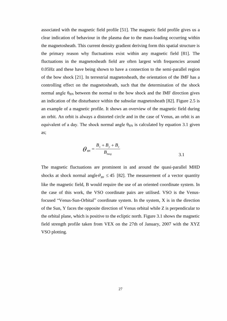
the orbital plane, which is positive to the ecliptic north. Figure 3.1 shows the magnetic
field strength profile taken from VEX on the 27th of January, 2007 with the XYZ
VSO plotting.
28
6.3337 6.3337 6.3337 6.3337 6.3337 6.3337 6.3337 6.3337 6.3337 6.3337
x 1013
0
50
100
Bm
ag
6.3337 6.3337 6.3337 6.3337 6.3337 6.3337 6.3337 6.3337 6.3337 6.3337
x 1013
-100
0
100B
x
6.3337 6.3337 6.3337 6.3337 6.3337 6.3337 6.3337 6.3337 6.3337 6.3337
x 1013
-100
0
100
By
6.3337 6.3337 6.3337 6.3337 6.3337 6.3337 6.3337 6.3337 6.3337 6.3337
x 1013
-100
0
100
Bz
Time in ms
Figure 3.1 Magnetic field strength (B) for 27th January, 2007.
Where;
Bx, By, and Bz represents the magnetic field strength in the X, Y, and Z VSO
directions respectively. Bmag is the magnitude of the magnetic field components which
can be derived by equation (3.2);
)( 22
zyx BBB 2magB
3.2
“The orientation of these waves can be analysed using a variance analysis of the
magnetic field components.” [52] This analysis is carried out with the minimum
variance method in this work. For any orientation of the IMF and location within the
magnetosheath, the magnetic field of the magnetosheath is generalised. The
generalised uniform magnetic field is a result of the three Cartesian components,
which are treated as separate vector in the presence of the flow field velocity.
Deriving from equation 3.2, the linear superposition is justified since the magnetic
field due to each of the field components is a solution obtained from a pair of
simultaneous differential equations [2] [52]. The divergenceless B and Faraday‟s law

29
seen in table 2.3 fulfil these conditions since they are linear and homogeneous in B.
They are repeated respectively in equation (3.3) and (3.4);
Div B = 0 3.3
The other is in Gaussian units;
E
t
B
c
1
3.4
With c representing the velocity of light in a vacuum that is sufficiently small, and the
tB is zero, the steadiness of the reference frame is confirmed. This can be
explained with regards to the divergenceless requirement, which implies all magnetic
field lines must eventually close on themselves [2]. The field line is that curve that
remains parallel to the resident magnetic field direction. Thus no matter the deviation
or fluctuation experienced in a magnetic field, it remains self consistent. Hence, while
a quasi-parallel shock, which occurs when BN 45°, causes turbulence in the
plasma, the quasi-perpendicular shock at BN 45° results in a jump of plasma
parameters between the upstream and downstream regions. [21][ 2] In the quasi-
parallel shock, the magnetic field crosses the shock plane, and by so doing cause the
charged particles to gyrate along the field lines. This makes it possible for the
particles to be easily taken across the shock. The magnetic field lines are nearly
parallel to the shock plane in the quasi-perpendicular case. As a result the gyration of
the particles along the magnetic field does not cross the shock directly. With the
gyrated motion, the charged particles are conveyed to the front of the shock [2]. For
the quasi-perpendicular shock, Angsmann et al [61] hold that it is not always true that
the spacecraft entry into the magnetosheath can be recognized from the reduction in
the wave activity. They contend that for quasi-perpendicular shocks, the wave activity
become heightened due to the invasion of the magnetic barrier by the magnetosheath
waves.
3.3. MINIMUM VARIANCE ANALYSIS

30
The analysis of the orientation of the vectors responsible for the magnetic fluctuations
occurring in the magnetosheath is achieved in this project by the minimum variance
method. In situations where the statistical characteristics due to measurement error or
the a priori error in evaluated quantity is not available when the least square and
weighted least square methods are used; the minimum variance approach can be
effectively utilized. According to Sonnerup et al [83], this technique can be applied to
the analysis of magnetic field vector data measurement for a spacecraft crossing a
transition layer (the magnetosheath in this case). The method is based on a theoretical
one dimensional model of the magnetosheath such that, in the coordinate system of 3-
dimension, only one remains when the divergence of the magnetic field B is
evaluated. That is in the 1-dimensional system, where 0 x and 0 y , then
equation 3.5 suffices for the divergence of B;
0.
z
BB z 3.5
Equation 3.5, projects Bz as being independent of z such that in a 3-cartesian system,
in the z-axis direction, the vector of interest points in the normal of the transition
layer. Since we are using the VSO coordinate pair and direction, the sort normal will
be in the direction of x. It can be established by equation (2.3) (Faraday‟s Law-
tBE ) that since the magnetic field B is not time dependent, then the field
component – Bx in the VSO coordinate system will be independent of time. That
means the relationship, 0 tBz is such that the traversing spacecraft will
experience a rigorous constant of Bx. This is important as it indicates that when a
spacecraft crosses the magnetosheath boundaries severally, the value of Bx is
observed to be the same. Thus using three vectors measured from the spacecraft, the
normal can be determined by its field not changing frequently. The assumption made
in this idealised 1-dimensional field is that given three vectors (B1, B2 and
B3), nBnBnB
321 , where )()( 3221 BBBB are the tangential to the shock
layer. Using equation 3.6, the cross product of the tangents can determine the normal
direction, provided they are not zero.

31
)()(
)()(
3221
3221
BBBB
BBBBn
3.6
In reality, the large amount of data, the spatial fluctuations noticed in the normal of
the transition layer and the presence of internal structures given in 2-dimensional or 3-
dimensional space create a complicated case. However, the minimum variance
method can deal with these non-ideal effects and provide good results. In order to
estimate the normal from a set of field-component set, B(m)
(where m=1, 2,3,4,…), the
minimum variance method locates of the normal direction in space as the vector with
the minimum variance. This happens to be represented as the minimisation carried out
in equation 3.7;
2
1
2 )(1
M
m
m nBBM
3.7 [83]
Where, the average B is defined by
M
m
mBM
B1
)(1 3.8
Due to the non-ideal circumstances, a Lagrange multiplier, λ can be introduced with a
minimisation carried out under a normalisation constraint 12n
. The implementation
of this constrained minimisation can be realised by the solution of a set of
homogeneous equations akin to those suggested by GCDF model represented in
equation (3.9);
0))1((22
n
nx
0))1((22
n
ny
3.9
0))1((22
n
nz
Where σ2 can be obtained from equation 3.7 and n
is represented in terms of its
components (nx, ny, nz) in the VSO coordinate system. The differentiation of the
equations in equation 3.9 leads to three equations that are represented in matrix form
by equation 3.10;

32
nnM v
v
B
v
3
1
3.10
Where μ, v =1, 2, 3, are the component of the field components in the X, Y and Z
axis. The magnetic variance matrix B
vM can be obtained using equation (3.11);
vV
B
v BBBBM 3.11
The resulting three eigenvalues and corresponding eigenvectors obtained by solving
the magnetic variance matrix as can also be seen in equation (3.9). The eigenvalues
are real because of the symmetric nature of the magnetic variance matrix. The
corresponding eigenvectors are the maximum, intermediate and minimum variance of
the field component.
The eigenvector which corresponds to the smallest eigenvalue is used for the
determination of the vector normal to the magnetosheath field. The smallest
eigenvalue is the reflection of the variance of the magnetic field component in the
direction of the determined normal. Overall, the resultant minimum eigenvalue and
eigenvector obtained for any measured set of vectors obtained from the traversing
spacecraft provides a system for the display and analysis of the data. Mathematically,
the direction of the minimum variance in the magnetic field is found using spectral
method, by solving the eigenvector corresponding to the minimum eigenvalue of the
spectral matrix (covariance). The calculated normal direction is assumed to be the
dominant direction of propagation of the wave vector. Espley et al [84] cautions on
the use of the minimum variance analysis especially in regions of nearly linear
polarization. In these areas the linear polarised waves causes the estimated minimum
and intermediate eigenvalues to be very similar. The standard deviation according to
Luhmann et al [21] during each averaging interval is obtained using the relation in
equation (3.11); the use of y and z component may be due to the deviation that they
set into the B at the subsolar direction of the solar wind flow.
22
zy BBB 3.12

33
3.4. TIME SERIES: SPECTRAL SCALING, TIME RESAMPLING AND
WAVELETS
Most space plasma physics data is almost entirely in the form of time series; hence its
analysis necessitates the manipulation of the time series. The VEX magnetic field data
has the same characteristics, thus the analysis of the profile for the results in this work
will involve the synthesis of time dependent magnetic profiles. Since physical theories
and models are formulated in frequency and not in time, there is the need to transform
the time series to the necessary frequency domain. This transformation of the time
series to the related frequency domain and application of statistics in the result is
spectral analysis. The objectives of using spectral analysis generally include model
building; using developed model and analysis of frequency attributes of the modelled
process/system. According to Chatfield, [70] to effectively analyse a time series,
description, explanation, prediction and control are important objectives.
1. DESCRIPTION
This is the first step in the analysis of a time series. It involves the plot of the
observation against time. This aids the description of the primary attributes of the
series. The description of „obvious‟ features such as trend and seasonality can be
perfectly achieved by these time plots. Such time plots will also show outlier - those
that do not appear to be consistent with the other members of the data set. Robust
methods such as wavelets transform is designed to be insensitive to outliers. Abrupt or
gradual changes, points of inflexion and any form of discontinuities are some of the
properties of a time series that we can easily identify using time plots.
2. EXPLANATION
The observations noticed in several variables such as variations in a particular time
series can be used to explain the processes in another series. Such comparison can be
instructive in providing an in-depth understanding of the source of a given time series.
Models are often applied to the explanation of a process using variations from another
variable.
3. PREDICTION
34
In forecasting and in the analysis of most time series, it is necessary to predict the
future values of a series. In prediction, the estimation of future values )( Ttx of the
time series is carried out in some future range lT 0 . It is easy to capture the
characteristics of a time series and use these observed features to estimate or
determine the future. Generally, most series takes an additive or multiplicative form.
These can be seen in the decomposed form below;
Series = trend + seasonal +irregular 3.13 [85]
The irregular component in this additive pattern of time series represents non-
systematic changes in the series. A multiplicative form of time series can be
represented in the following:
Series = trend x seasonal x irregular 3.14 [85]
Since the forecast of future observations are a result of extrapolation, the mean
square errors associated with them must be calculated.
4. CONTROL
In processes where there is the need to carry out some control, the analysis of a time
series is used to improve control over such physical systems. Control problems bear a
correlation with prediction in many situations. Most of the approaches to improving
the performance of a system by time series manipulations include the fitting of
models to the series. These strategies enable the prediction of a target in the future so
that the necessary process variables can be suited to meeting them.
3.4.1. SPECTRAL ANALYSIS
Spectral analysis is a useful tool for the diagnostic analysis of different types of time
series. It is concerned with estimating a spectrum over a whole range of frequency.
Spectral analysis engenders three very important theoretical approaches, this includes
– the statistical analysis of time series, wavelets transforms and the Fourier analysis.
In the statistical analysis, the concern is on how to analyse the collected data and how
to use the analysed results in making sensible real life consideration. The

35
development of a general approach that deals with data analysis can be achieved
either as a test of significance or an estimation theory. The test of significance
examines a data to see if it is consistent with a specific hypothesis using a random
variation. In the estimation theory, the data is used to determine the value of the
parameters in an assumed probability distribution function, and to evaluate how
accurate the error is. The computation of the mean and variance for different time
periods in order to see how significantly different they are, makes statistics the
simplest method for analysing non-stationarity of a time series. The defects associated
with the use of statistical time plot is that they suffer from time localization (curve
shape is dependent on the length of the window used, thus a compromise always has
to be chosen between strict amount of smoothening and or too-little) and frequency
localisation (here the running variance has no data on the frequency of a periodic
signal- it only has its amplitude).
One possible way of dealing with these defects is to use the windowed (or running)
Fourier transform (WFT). WFT involves “the use of a definite window size and
sliding it in time, together with the computation of the Fast Fourier Transform (FFT)
at the corresponding time based on the data within the window.” [70, 79]
3.4.2. FOURIER ANALYSIS
This technique of spectral analysis involves the estimation of a function by a sum of
sine and cosine terms. Suppose a function representing a process )(tu is defined over a
finite time span Tttt oo ; then )(tu can be approximated over the time span such
that Fourier theorem states that for a finite and piece-wise signal, the series can be
approximated by the Fourier series (provided the function )(tu is reasonably behaved
within the time span – that is it satisfies the Dirichlet conditions)
)2exp(][~)( tifnutu n
n
3.15
Where each term in the Fourier sum corresponds to an oscillation at a frequency nf
which determines the time scale of the signal

36
Tnfn / 3.16
and the complex Fourier coefficient ][~ nu is approximated as
dttiftuT
nu n
Tt
t
o
o
)2exp()(1
][~
3.17
Since the oscillation nf is an eigenmode which corresponds to small-amplitude
disturbances for most geophysical systems, it is a means of discerning the physics of a
signal. The expression in equation 3.17 is a finite interval. It is the replacement of a
continuous infinite value of )(tu with span Tt 0 by an infinite series of ][~ nu for
all integers n . Since in most cases, the data from the measuring instruments are
provided in a sampled order, the continuous function )(tu is replaced by a discrete set
of N measurement using Discrete Fourier Transform (DFT).
Generally, the emergence of the spectral density as a method to spectral analysis
stems form the inability to integrate stochastic processes with an absence of a Fourier
transform that converges. The two forms of the spectral analysis are the Power and
Cross spectral density. The Parseval‟s relation / theorem provides the physical
representation of a Fourier series over time by describing the total energy contained in
the signal in terms of Fourier transform of the waveform summed over all the
frequency constituents. The relation
n
Tt
t
nudttuT
o
o
22 ][~)(1
3.18
For a real signal, 3.18 becomes
1
222 ][~2]0[~)(1
n
Tt
t
nuudttuT
o
o
3.19
The power spectral density (PSD) is the description of the signal energy density
distribution in the frequency domain by the introduction of a function uS to the
Parseval‟s relation. Hence, equation (3.19) takes the form

37
fnSf
SdttuT n
uu
T
][2
]0[)(1
10
2 3.20
Where the frequency spacing T
f 1 and the function 2
][~2 nuTSu .PSD is
applied only to real signals as negative frequencies are ignored. It is the contribution
to the signal energy from the frequency interval 1f around nf . The cross spectral
density on the other hand is the Fourier transform of the cross-correlation function.
However this work will not be delving into this. Parseval‟s relation enables the
interpretation of each of the terms in equation 3.19 with regards their contribution to
signal strength at the corresponding oscillation frequencies nf . Applying the magnetic
field within the magnetosheath as the signal )(tu , the related physical energy
contribution of plasma in the various locations of the ionosphere can be interpreted.
Hidden periodicities can be discovered using the periodogram by the application of
the Parseval‟s relation. The periodogram usually refers to a plot of signal (a function
of frequency) against frequency. The total area which it covers is equal to the variance
of the time series [70]. Detailed information for Fourier analysis and its methods can
be found in [70][79][86].
3.4.3. WAVELETS
Wavelet analysis derives from the need to solve problems based on the inconsistency
discovered in the treatment of time series by the various Fourier analysis methods.
The nature of wavelets is likened to a periodic signal that starts from the origin,
reaches maximum displacement and then end again in the origin. It seeks to solve
time series problems by breaking down the signal into its time/frequency domain
simultaneously. Wavelets allow the observer to obtain information about the
maximum displacement within a signal together with the variation of the amplitude
with time. “The wavelet transform can be used to analyse series that contain non-
stationary power at many different frequencies”. [87] Wavelets possess a zero mean.
Deriving from the Heisenberg‟s uncertainty principle, wavelets are distinguished by
the nature of localization between the time ( t ) and the frequency/bandwidth ( w ).
[88] Thus, the precise localization of one of these properties reduces the precise

38
control over the other. Wavelets operate by expanding a signal in basis function, the
function which is restricted in time and frequency ensures that they posses wave
packet features. They are finite in extent with respect to duration and specific
frequency as such; wavelet has characteristics that lie between Fourier techniques and
pure time series representation. [86]
The special combination of balancing time and frequency which wavelet possesses
can be visualised in the Morlet wavelet shown in figure 3.2 and represented
mathematically in equation (3.21).
Figure 3.2 Morlet wavelet of arbitrary width and amplitude with time along x-axis [90].
Figure 3.3 shows how the Morlet wavelet incorporates periodicity and finiteness in its
formation. The figure depicts the multiplication of a sine wave (with its periodic
properties) by a Gaussian enclosure (which does the time localization). [90]
Figure 3.3 Construction of the Morlet wavelet (blue dashed) as a sine curve (green) modulated by
a Gaussian (red). [90]
The Morlet wavelet is defined as
2/41
0
20)( ee
iw, 3.21

39
0w and are the dimensionless frequency (wavenumber) and time respectively.
)(Psi is the wavelet value at 0w and . This basic wavelet function is normalized to
ensure that it has unit energy when compared with to wavelet transform from other
time series. The normalisation involves the scaling of the wavelets by weighting of
the amplitude of the Fourier coefficients. The normalisation or “scaled wavelet” is
obtained using the scaled version of (3.20) in the convolution of the time series
(discrete sequence) nx . The inner product of nx is (3.22)
s
tnnxsW
N
nnn
)(*)(
'1
0'
' , 3.22
(3.22) “is the continuous wavelet transform (CWT) of a time series nx ”. [79] Where
(*), s and n represents the complex conjugate, wavelet scale (constantly changing) and
the time index on which the translation occurs. “The wavelet transform is simply the
convolution between a time series nx and the wavelet value )(Psi ”.[90] The
normalization using equation (3.22) is
s
tnn
s
t
s
tnn
)()( '
0
21'
, 3.23 [79]
Where 0 is the un-scaled wavelet value, and the normalization of )(0 leads to it
having unit energy. The wavelet transform has a real, )}({ sWn and imaginary
part )}({ sWn . They both translate to the amplitude ( )(sWn ) and phase
(
)}({)}({
sWsW
n
n) respectively of the wavelet function. The wavelet power
spectrum is indicated by2
)(sWn . Torrence and Compo [79] used the wavelet analysis
to obtain the frequency and amplitude of warm and cold events for a period of 120
years.
The choice of the wavelet function )(0 to be used is discretionary and it depends
on

40
The shape of the wavelet – that is the mother wavelet (Morlet, Paul, DOG)
should be characteristic of the time series.
Complex or real – For instance in the capture of oscillatory features, a
complex wavelet function can be applied since it can effectively isolate peaks
and discontinuities
Orthogonal or nonorthogonal – Nonorthogonal wavelets are applied to discrete
sequence where smooth and uninterrupted changes are expected. The reverse
is applicable for orthogonal analysis since the functional analysis of the
wavelet basis increases with the width at a particular scale.
Wavenumber and wavelet scale – the wavenumber 0w determines the number
of cycles in the wavelet and impacts on the error. The relationship the scale
bears with the Fourier period means it must be calculated in consideration of a
suitable wavelet function. The scale itself determines the smoothness that can
be achieved; it is limited in the orthogonal wavelet but arbitrary in the
unorthogonal form. The selected scale is expected to be smaller than half the
distance covered by the time series.
Reconstruction – The wavelet is a filter with a known response. This feature is
necessary in the choice of the wavelet function as will be observed in this
work and as can be seen in figure 3.4 and figure 3.5 respectively
6.3347 6.3347 6.3347 6.3347 6.3347 6.3347 6.3347 6.3347 6.3347 6.3347 6.3347
x 1013
0
10
20
30
40
Unclean Bmag
Plot of Data
6.3347 6.3347 6.3347 6.3347 6.3347 6.3347 6.3347 6.3347 6.3347 6.3347 6.3347
x 1013
-5
0
5
10
15
20
25
Cleansignal Plot of Compressed value of BMag
Unclean Signal
Clean Signal
Figure 3.4 Decomposition of magnetic profile on May 23rd
, 2007 using Daubechies6 wavelet

41
6.3347 6.3347 6.3347 6.3347 6.3347 6.3347 6.3347 6.3347 6.3347 6.3347 6.3347
x 1013
0
10
20
30
40
Unclean Bmag
Plot of Data
6.3347 6.3347 6.3347 6.3347 6.3347 6.3347 6.3347 6.3347 6.3347 6.3347 6.3347
x 1013
0
5
10
15
20
25
30
Cleansignal Plot of Compressed value of BMag
Unclean Signal
Clean Signal
Figure 3.5 Decomposition of the magnetic profile on May 23rd
, 2007 using Haar wavelet
Width – The resolution in wavelet transform depends on the ratio of the width
of the original space to the width of the wavelet function in the Fourier
domain.
Cone of influence – This is important when considering the zero padded
wavelets with large scale. It deals with the autocorrelation due to edge effect.
3.4.4. FOURIER TRANSFORM METHODS AND WAVELET COMPARED
An implicit problem found in Fourier analysis is the treatment of time series as
stationary. This is tasking since most Geophysical time series are non-stationary. The
effect is that the traditional methods of Fourier Transform are defective from start in
dealing with the complexities found in these data. The Windowed Fourier Transform
for instance is ineffective when the time-frequency position of a time series signal is
involved. WFT is performed on a time series of length tN , with a time step of t .
With a sliding segment of length T, the transform is inefficient as a result of
relation )2/( tT that must be analysed at each step. This is irrespective of the window
size as such; the inaccurate result means a scale has to be introduced. [79] The
presence of aliasing from the high and low frequencies which does not fall within the
window is the origin of the inaccuracy that is characteristic of the WFT. The
inconsistency in the treatment of frequencies which accounts for the inaccurate result
is explained at low frequencies by the so few oscillations within the window. At high
frequencies, these results contain so many oscillations, thus making them inaccurate.

42
The numerous oscillations at high frequencies means that time localization is lost
within the window, while the frequency localization is lost at low frequencies. There
is also need to analyse several window length in order to determine the right option.
“The wavelet transform is appropriate for the determination of analysis where the
range of the dominant frequencies make it difficult to apply predetermined scaling”.
[79]
The Short Time Fourier Transform (STFT) was developed to overcome the inability
of Fourier transform to tell when in time the frequency component are located.
However, it is unable to differentiate the different spectral parts that exist at different
points of time. It only provides information on the time interval in which a particular
band of frequencies exist. STFT has a poor frequency resolution. The continuous
wavelet transform (CWT) is an alternative to the poor resolution of the STFT. It
provides a robust solution to the resolution dilemma by applying the transform
separately to different segments of the signals. This it achieves by changing the
window width for every single spectral part.
Generally while Fourier decomposition is applicable to situations where smoothing
and random walk data are considered, Wavelets are most useful in defining bursting
and flat data. [94]
3.5. TREND AND GRADIENT MODELLING
In the use of spectral analysis as a diagnostic tool of the fluctuations due to the
magnetosheath of Venus, the periodogram has to be smoothed in order to obtain a
coherent estimate of the background spectrum. The removal of the trend is the
prewhitening going by the goal and procedure used in the process. This removal is
achieved by taking a linear transformation of the raw data so that they do not cause
any twisting to low frequency part of the spectrum [70][86]. The resulting spectrum
which represents the original series can then be estimated. In this work, the parametric
approach of autoregressive models (AR, ARX, ARMA, ARIMA) and vector
autoregressive (VAR) model have been used to mimic the characteristic gradient of
the Venusian magnetosheath. Detailed information on these linear modelling
techniques can be found in [4], [28], [70], [73] and [85]. A linear or quadratic

43
function is fitted to the trend within the magnetosheath. They are not resolved by the
spectrum analysis methods discussed here due to their time scales being longer than
those that can be contained within the spectral analysis data. There are three
approaches to dealing with trends, these includes filtering, differencing and curve
fitting. The trend described by the globalised linear equation in equation (2.5) has
features that most times do not explain the underlying data. A deterministic model
which assumes and as rising stochastically is most suitable in most cases since
it allows a smooth evolution through time between the model parameters - and
in this case. Non-linear models can be used for the description of the trend, and the
non-linear trend form can be evaluated using quadratic or exponential growth. This
work will be restricted to the linear trend models. It must be noted though that the
analysis of trends is dependent on the goal for the analysis. This may be simply to
measure the trend or the removal of the trend in order to describe local variations.
Seasonality in the data also determines the trend analysis approach used. Descriptions
of the three approaches stated earlier are considered below.
3.5.1. CURVE FITTING
This traditional method lends itself to trends in non-seasonal time series particularly
around data. It involves the simple fitting of a polynomial curve, a logistic or the
Gompertz curve to function in equation (2.5). The globalised linear trend is a good
example of a polynomial curve. The Gompertz curve can be represented by the
general form
t
t brax log 3.24
Where a, b, r are parameters lying between 0 and 1. The logistic curve comes in the
form
)1( ct
t beax 3.25
The s-shaped logistic and Gompertz are asymptotic as t . The Gompertz curve
best serves in non-linear trend fitting.

44
3.5.2. FILTERING
This is simply the linear transformation of the time series into another by a linear
operator. Normally this can be written in the form
rt
s
qr
rt xay
3.26
Where ra is a set of weight; ty is the new time series and tx is the original data set. A
moving average (MA) that uses the average estimate of the weights, ra , such that the
sum of the weights equals „1‟ that is 1 ra is an example of the operation carried
out in filtering. By the effect, it ensures the smoothing out of local fluctuation by
averaging. “Moving average is often symmetric” [79] and they introduce end-effect
problems to the filtering process. When the trend analysis is for the purpose of
forecasting, an eye or asymmetric filter that project smoothed values up to t=N is
used. Exponential smoothing is an example of such filters. It works with the premise
that
t
j
j
tm xxS
0
)1()( 3.27
Where is a constant that lies between 0 and 1, with the weights j
ja )1( .
This weight reduces with j geometrically. )( tm xS is the smoothed value. The selection
of the filter is governed by the “experience and knowledge of the frequency aspects of
time series analysis” [79].
3.5.3. DIFFERENCING
This is the process of removing a trend form a time series until it becomes stationary.
The scheme adopted is fully integrated into Fourier techniques especially in the Box-
Jenkins procedure. The goal here is simply the formation of a new series from the
original time series. Where the new series is represented by ty and tx is the original
series, differencing can be formed by

45
ttt xxxy 1 For t=2, 3,…, N 3.28
In certain situations, a second order differencing is applied to model the trend. The m-
file „mytrend.m‟ in the Appendix, applies differencing.
3.6. SUMMARY
This chapter has presented the basic theory guiding the use of the gradient method of
analysing the data from a spacecraft traversing plasma material. The minimum
variance method for the analysis of the magnetic fluctuations in the magnetosheath
was also discussed. Similarly the magnetic field distribution and the adopted VSO
coordinate system are also discussed. The methods of Fourier transform and wavelets
as well as their use in the manipulation of time series data are also given considerable
attention in this chapter. The chapter ends with a discussion of the different
approaches to modelling trend and gradients in data.

46
Chapter 4 - EXPERIMENTAL PROCEDURE AND
IMPLEMENTATION
4.1. INTRODUCTION
Following from the background provided in the previous chapter, this chapter is
devoted to the exposition of the techniques and procedure deployed in the
determination of the trends and gradients of the Venusian magnetosheath. It explores
the ideas earlier discussed in this work while explaining the basis for the choices
made at various steps in the procedure. The first section of the chapter describes the
nature of the unique VEX data and how this affects the decisions regarding the
manipulations used in the work. It also presents the method that has been adopted in
identifying magnetosheath crossings within the ionosphere of Venus, as well as their
characterisations. Other sections of the chapter describe the procedure used in
determining the trend and gradient of the Venusian magnetosheath.
4.2. NATURE OF UNIQUE VEX DATA AND TREATMENT
The unique VEX data is obtained from the magnetometer (MAG) and plasma
instrument (Automatic Space Plasma Experiment with Rotating Analyser –
ASPERA). [95] ASPERA, which is a ion-mass spectrometer, uses a “combination of
measures from the naturally occurring fields of venus and those due to the stray field
produced from the operation of VEX”. [52] The role of the twofold sensor ensures
that the effect of the stray field on the measurement can be identified and removed,
hence, VEX which is otherwise a magnetically “unclean spacecraft” gives rise to
clean magnetic profile. This is achieved by the application of artificial magnetic field
of ±10,000nT to each sensor for compensation of any disturbing spacecraft stray
field.”[96] The stray field is a result of the magnetometers being located on the solar
panel; in effect, Electronics currents produced on board the spacecraft is detected.
[84] The 1 Hz data set with a time resolution of 1s for a full three-dimensional
distribution is used for this work. “The time resolution is necessary because of the

47
rapid crossing of different structure in the magnetic data set, thus it ensures that
reliable statistical results is obtained.” [59] The magnetic data is obtained via the ion
mass analyzer (IMA) on VEX. IMA “measures particles in the energy per charge
range 0.01-3.6keV with a field of view 90 x 360;” [52] the data set is received in
BAM data („*.dat‟) form. Figure 4.1 shows a cut away version of the orbiter
instruments on VEX.
Figure 4.1 A cutaway diagram showing size and locations of Venus Express instruments. [97]
Each data set is recorded on a 24hours basis equalling Venus/VEX orbit length. The
data is pre-processed using matlab program. The process involves extracting the daily
orbit data from the BAM data and converting them to “*.mat” format to improve the
efficiency of the process as well as reduce the time used in reading the data. The
converted BAM data is then read to reveal the Venus Express 1Hz magnetic field
data. The pre-processed data is presented in a structural array called „fgm‟. fgm
contains data and flags. The structural fgm is shown below for the 27th
of May, 2006.
Figure 4.2 contains a typical content of the information in the structural fgm. In each
of the fgm data set, there are fifteen (15) parameters about time (UTC, OBT, MS,

48
StartUT, …) and magnetic data (BIS and BOS).
Figure 4.2 fgm data structure containing data and flags
In this work, the emphasis is on using the magnetic data to reach our set objectives.
The magnetic part of the data comes in terms of the VSO position in kilometer (km)
and the magnetic part measured in nano Tesla (nT).
4.3. DATA SCREENING AND HANDLING
This report considers BAM data collected from VEX from the 1st of January, 2009 to
the 28th
of February, 2009 – a total of 59 data sets. In reading the original BAM data,
a choice has to be made on how abnormal values (due most time to missing data) will
be treated. There are various approaches available in such treatment; this is either to
replace the value with the previous good value in the data; deleting the affected
variables or data; estimating the missing data by interpolation; using a joining
algorithm like those in „catstruct.m‟ that concatenate the disjointed parts, or the use of
the matlab not a number (NaN) to replace such values. These abnormal values can be
visualized as flags represented by 99999.999. J. Du et al in [98] adduced their
presence as resulting from the data cleaning process. Zhang et al [63] reports that the
2-4minutes of missing data noticed was owing to the saturation of the inboard sensors
from time to time. Specifically, they hold that “the inboard sensor will be saturated

49
about two to four times per day due to the switch on/off of antenna transmissions, and
the solar array driving mechanism (SADM) changing the angle of the solar panels”
[63]. Since these gaps could alter the generalisation reached, this work has shown that
the method chosen for the re-sampling of the gap can be crucial to the modelling
effort as well as place outliers in the model estimates. The choice made here is to
interpolate the missing data cases using a string metaphor, though they show a
random pattern when the modelling is involved. The method used is so that there will
be continuity and 24-hours plot of the magnetic field. Figure 4.3 shows the effect of
the method for the data set of the 29th
of January, 2009.
Figure 4.3 Replacing NaN/Missing Data in Magnetic Field Profile_090129
4.4. LOCATING THE POSITION OF THE MAGNETOSHEATH CROSSING
In chapter 2, it was explained that the spacecraft (VEX) orbits about Venus and
during each orbit, the magnetosheath is crossed twice as seen in figure 4.4;
Figure 4.4 Example of an orbit [99]

50
Figure 4.4 shows that in orbiting around Venus; VEX transverses through the
magnetosheath during the nightside and dayside; the crosses are from the nightside to
the dayside and from the dayside to nightside respectively. As earlier noted, the
dayside ionosphere contains the most important information that relates the solar wind
interaction with Venus, thus the emphasis of this work will be focussing on the data
obtained during the crossing of the magnetosheath in this region. The choice of the
dayside is further accentuated when one considers that the subsolar region of the
atmosphere of Venus as seen in literature review and basic theory as well as in figure
4.4, occur in the direction of the x-component. Since plasma in space show changes
when they encounter obstacles in space, this idea is used in the selection of the region
relating to the magnetosheath crossings. As observed by Zhang et al [96], the crossing
due to each physical region of the Venusian atmosphere is recognizable by the
changes in the strength of the magnetic field and the wave/fluctuation activity related
to it. The selection criterion of the magnetosheath criterion is that the field direction
while the spacecraft is inside the magnetosheath, does not change drastically after the
sudden change noticed when VEX crosses the bow shock [21], [74] and [99]. The
“frozen” magnetic field of the magnetosheath can be visualised following the
determination of the dayside bow shock - “which is the region due to the inflexion
from negative to positive in the X-component of spacecraft position” [99]. A typical
orbit of VEX and the determination of the magnetosheath crossing is shown in figure
4.5 and figure 4.6.
Figure 4.5 Magnetic Profile showing location of magnetosheath

51
6.3347 6.3347 6.3347 6.3347 6.3347 6.3347 6.3347 6.3347 6.3347 6.3347 6.3347
x 1013
-30
-20
-10
0
10
20
30x-component of B 090129
6.3347 6.3347 6.3347 6.3347 6.3347 6.3347 6.3347 6.3347 6.3347 6.3347 6.3347
x 1013
-6000
-4000
-2000
0
2000
4000
6000direction of x-component
solar windSolar wind
magnetosheath
s
h
o
c
k
Figure 4.6 X-component trajectory of spacecraft position and the shock (Area marked in red)
The exit from the magnetosheath by VEX is observed by the return of the magnetic
profile to pre-obstacle patterns (see figure 4.6). The magnetosheath location is
extracted and examined. The magnetosheath region on the 9th
of January, 2009 is seen
in figure 4.7; the time between when the spacecraft enters the magnetosheath to its
exit is observed to be within 70s in this study.
6.3347 6.3347 6.3347 6.3347 6.3347 6.3347 6.3347 6.3347 6.3347 6.3347 6.3347
x 1013
-50
0
50
Bz
6.3347 6.3347 6.3347 6.3347 6.3347 6.3347 6.3347 6.3347 6.3347 6.3347 6.3347
x 1013
-50
0
50
By
6.3347 6.3347 6.3347 6.3347 6.3347 6.3347 6.3347 6.3347 6.3347 6.3347 6.3347
x 1013
-50
0
50
Bx
6.3347 6.3347 6.3347 6.3347 6.3347 6.3347 6.3347 6.3347 6.3347 6.3347 6.3347
x 1013
0
20
40
Bmag
6.3347 6.3347 6.3347 6.3347 6.3347 6.3347 6.3347
x 1013
-50
0
50
Bz
6.3347 6.3347 6.3347 6.3347 6.3347 6.3347 6.3347
x 1013
-50
0
50
By
6.3347 6.3347 6.3347 6.3347 6.3347 6.3347 6.3347
x 1013
-50
0
50
Bx
6.3347 6.3347 6.3347 6.3347 6.3347 6.3347 6.3347
x 1013
0
20
40
Bmag
Figure 4.7 Magnetic Profile showing; (a) 24 hrs orbit. (b) Within Magnetosheath
4.5. IMPLEMENTATION
Here the characteristic of the magnetosheath is investigated. Properties such as the
shock normal angle, clock angle, the normal direction, altitude, amplitude, wave

52
vector direction and frequency are investigated. The mean field method is adopted in
gaining the insight of the 59 data set. The approach involves carrying out the
procedure for each data set, binning the result and proceeding to use the output
statistics to compute the overall characteristics shown in the region.
4.5.1. MINIMUM VARIANCE ANALYSIS AND SHOCK NORMAL ANGLE
It has been established in chapter three that, the application of the Minimum variance
analysis technique ensures that we can determine the direction along which the
variation of the magnetic field is minimum. [83][100] The normal vector is calculated
in matlab and the direction of the normal noted. The matlab code „minvar.m‟ is used
for the purpose. The implementation of the minimum variance is summarised to
involve the construction of the variance matrix (described by equation 3.11) -
vV
B
v BBBBM . The eigenvalues and the corresponding eigenvectors of
the matrix is obtained and utilized in determination of the direction of minimum
variance. The minimum variance is an indicator of the normal direction discussed and
represented by equation (3.6), the normal direction. A comparison of the eigenvalue
due to the minimum variance with the other eigenvalue can give an indication of the
estimated normal direction. If the difference is large between these values and the
minimum variance eigenvalue, then the estimation is a good determination of n
.
Precautions in the application of this estimator as raised by Sonnerup et al [83] and
Espley [84] is considered. The steps taken in the calculation are summarised by J.
Wang in [100] to include;
Calculate the average value, Hi for the components of B – that is the mean of
Bx, By and Bz. For instance – H1=mean(Bx);
Calculate the differences between each component and the mean value. Get
the mean value of the result; For example, where, X11 = Bx – H1;
H11= mean(X11);
H11 corresponds to the last term of equation (3.11) - BB ;

53
Choose any two differences as a group and determine the variance. This
corresponds to the first term vBB in equation 3.11. Mathematically this
can be expressed as; xys=mean (X11.*Y22); xzs=mean (X11.*Z33);
yzs=mean(Y22.*Z33); xxs=mean(X11.*X11); yys=mean(Y22.*Y22);
zzs=mean(Z33.*Z33); Where Y22 and Z33 are the y and z component versions
of X11 respectively.
Obtain the variance matrix B
vM by computing vV
B
v BBBBM
The variance matrix is obtained in the following form;
111111111111
111111111111
111111111111
***
***
***
ZZzzsZYyzsZXxzs
ZYyzsYYyysYXxys
ZXxzsYXxysXXxxs
M B
v
The smallest eigenvalue and the corresponding eigenvector are determined
from the variance matrix B
vM . The corresponding normal vector is estimated.
The procedure is repeated for all the data set.
Since the estimated normal is prone to error in the real world, there is a slight
deviation from the ideal situation where nBnBnB
321 , hence the estimated
normal is checked for consistency.
The shock normal angle BN is calculated using equation (3.1). This is in order to
reveal the nature of the incident solar wind on the bow shock. For the 9th
of January,
2009 the incident solar wind is > 45°, thus a quasi-perpendicular shock is present
during this orbit. The m-file „minvar.m‟ in Appendix gives a summary of the
minimum variance related attributes. The shock normal angle and clock angle for the
data sets considered can be obtained from the m-file „checking_normal.m‟.

54
4.5.2. GRADIENT OF VENUSIAN MAGNETOSHEATH
In chapter 2 and 3, the gradient was defined as the variation in the magnetic field with
respect to the position. Since the magnetic field strength is a scalar, the gradient
related to it gives us the idea of the irrotational field connected to it. For the fact that
the gradient of a vector is specified as the divergence of a curl, it is useful to
Helmholtz instabilities which explain the divergence of a curl to be automatically
zero. [2] Following from this, the magnetic field generated by steady or unsteady
current satisfies 0. B . In practise it has been proved that the electric charges
generated by static charges obey 0xE . This means that if we correlate the
relationship between the electric and magnetic field, there is a conservation of energy
involved. Hence, Faraday‟s law which relates the change between the magnetic field
and an electric current can effectively be said to be satisfied within the
magnetosheath. This is more so for a divergenceless B.
The determination of the variations in the magnetic field within the magnetosheath
when plotted on matlab does not provide all the information on the magnetosheath
column. It gives us an idea of the amplitudes of the magnetic field potential, but to
visualise the scalings and frequency attributes of the magnetosheath, spectral analysis
is required. Figure 4.8 is an example of the gradient obtained from the magnetic field
variation on the 9th
of January, 2009.
6.34 6.34 6.3401 6.3401 6.3401 6.3401 6.3401 6.3401 6.3401 6.3401
x 1013
-20
0
20
40
60
gradient of B-X component
6.34 6.34 6.3401 6.3401 6.3401 6.3401 6.3401 6.3401 6.3401 6.3401
x 1013
-40
-20
0
20
gradient of B-Y component
6.34 6.34 6.3401 6.3401 6.3401 6.3401 6.3401 6.3401 6.3401 6.3401
x 1013
-100
-50
0
50
gradient of B-Z component
Figure 4.8 Gradient due to magnetic field component on the 9th
of January, 2009.
The result shows that the gradient identifies with the points of perturbations within
Venusian ionosphere. Clearly, the data set shows the presence of anisotropy which is
related to the different profile that the various component of the magnetic field show.

55
Figure 4.9 depicts the gradient of Bmag with the use of the direction of minimum
variance (Z-direction) on that day applied to locate the magnetosheath location;
6.34 6.34 6.3401 6.3401 6.3401 6.3401 6.3401 6.3401 6.3401 6.3401
x 1013
-10
0
10
Gradient of Bmag
6.34 6.34 6.3401 6.3401 6.3401 6.3401 6.3401 6.3401 6.3401 6.3401
x 1013
-10
-5
0
5x 10
4 Direction of Minimum Variance - Z direction
6.34 6.34 6.3401 6.3401 6.3401 6.3401 6.3401 6.3401 6.3401 6.3401
x 1013
0
20
40
60
Bmag
Dayside
NIGHTSIDENIGHTSIDE
Figure 4.9 Gradient of the magnetic field on the 9th
of January, 2009, showing minimum variance
direction.
The gradient can be seen to be gyrating around the origin, with areas of peak and
minimum fluctuations shown. This means that, they obey the theoretical laws in table
(2.2).
4.5.3. TRENDS WITHIN THE VENUSIAN MAGNETOSHEATH
The presence of trends as a result of the fluctuations seen in the magnetic field of the
magnetosheath is achieved in this work by the removal of the best fit line of variation
within the magnetosheath. In the determination of the trend , the signal is localised to
the magnetosheath region. The purpose of the trend aside being part of the goal of this
work is also to remove the non-stationary part of the data so that we can have a
stationary signal that such that, it is easy to carry out a spectral analysis of the signal.
The advantage of knowing the trend of the signal in the magnetosheath also stems
from the need to determine the nature in which the variations in the magnetic field are
fashioned. Figure 4.10 is the trending of the entire orbit for the 9th
of January, while in
figure 4.11, the same are limited to the magnetosheath column alone.

56
6.34 6.34 6.3401 6.3401 6.3401 6.3401 6.3401 6.3401 6.3401 6.3401
x 1013
-10
0
10
20
30
40
50
60
Original Bmag
Trend
Detrended Bmag
Figure 4.10 Plot of Orbit of 9th
of January showing trends.
The „frozen‟ or semi-steady nature of the magnetosheath as enunciated previously in
chapter 2 can be viewed from this context.
6.3401 6.3401 6.3401 6.3401 6.3401 6.3401 6.3401
x 1013
-10
0
10
20
30
40
50
60
Original Bmag
Trend
Detrended Bmag
Figure 4.11 Plot of 9th
January showing the trend within the magnetosheath column.
In order to obtain the fine features of the magnetosheath region, the resulting de-
trended signal is manipulated with spectral analytical methods. However, the effect of
the trend can not be seen when the gradient of the signal is de-trended. As noticed in
figure 4.12, there is a zero trend in the gradient plot with the de-trended Bmag totally
superimposed on the original Bmag
6.34 6.34 6.3401 6.3401 6.3401 6.3401 6.3401 6.3401 6.3401 6.3401
x 1013
-8
-6
-4
-2
0
2
4
6
Original Bmag
Gradient
Detrended Bmag
Gradient
Trend
Figure 4.12 Trend in Gradient of the magnetic field on the 9th
of January, 2009.
Figure 4.13 restricts the orbital plot above to the magnetosheath alone;

57
6.3401 6.3401 6.3401 6.3401 6.3401 6.3401 6.3401
x 1013
-8
-6
-4
-2
0
2
4
6
Original Bmag
Gradient
Detrended Bmag
Gradient
Trend
MAGNETOSHEATH REGION IS SEEN
HERE
SHOWING A HEIGHTENED LEVEL OF
FLUCTUATIONS
Figure 4.13 Plot of the gradient showing nature of trend within magnetosheath on the 9th
of
January, 2009.
4.6. SPECTRAL ANALYSIS
The spectral analysis is applied to the manipulated data set to help reveal finer
features in the time-frequency domain. The known characteristics of the underlying
signal as discussed in chapter 3 will be considered in the application of the spectral
analysis method. The result from the manipulations due to the use of wavelets and
Fourier transform techniques is discussed here. It should be noted that in the treatment
with wavelet, the spectral scalings α, which corresponds to the Magnetic field was
estimated using Daubechies 6. With the nature of wavelets, there is no need to de-
trend the original data before applying the wavelet method. As described in chapter 3,
this is because of the filtering abilities of wavelets. Thus, since it has been established
that filtering is a process of removing trend, the trend identification here is self
consistent. The results obtained for the profiled region for both the Fourier technique
and those of the wavelets are compared.
4.6.1. WAVELETS ANALYSIS
In the analysis of the magnetosheath region using continuous wavelet transform; the
wavelet shape used, is the Daubechies wavelets. This is primarily because of the
orthogonal and efficient filtering properties they possess. In particular, finite data size
effects are reduced and the number of vanishing or edge moments can easily be
changed. The ability that Daubechies wavelets show in the handling of vanishing

58
moments distinguishes it from other wavelet function. This is especially in the
cancellation of the influence of polynomial trend or periodic structures in the data.
[74] The choice of db6 is based on the asymmetrical, smoothness, orthogonal and
biorthogonal properties. The db6 shape and the scaling factor associated with it are
shown in figure 4.14. The maximum level of decomposition of the signal is crucial to
the thresholding functions of wavelets as it imparts the robustness associated with
wavelets. There is a direct relationship between this level and the size of the signal.
Figure 4.14 The db6 scaling function and wavelet function. [101]
The matlab program to extract the time-frequency information in the magnetic field is
on the attached computer disk (CD). The process in the wavelet analysis involves the
following steps;
Performing a multilevel 1-D wavelet decomposition using the db6
(Daubechies 6) wave name.
De-noising the signal by extracting detail coefficients at level N from the
wavelet decomposition structure in (1) above.
The default values for the de-noising and compression process is returned
using wavelets or wavelet packets, of the input vector (the magnetic field data
in this case).
Generate a de-noised or compressed version „XC‟ of input signal „X‟. This
filtered signal is obtained by wavelet coefficients threshold. Soft thresholding
is applied in this work. The threshold values are fixed at exactly 6.000 for
each decomposition level, thus providing very good noise suppression. The
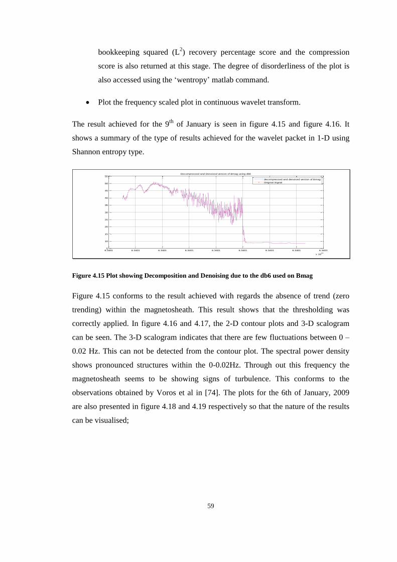
59
bookkeeping squared (L2) recovery percentage score and the compression
score is also returned at this stage. The degree of disorderliness of the plot is
also accessed using the „wentropy‟ matlab command.
Plot the frequency scaled plot in continuous wavelet transform.
The result achieved for the 9th
of January is seen in figure 4.15 and figure 4.16. It
shows a summary of the type of results achieved for the wavelet packet in 1-D using
Shannon entropy type.
6.3401 6.3401 6.3401 6.3401 6.3401 6.3401 6.3401 6.3401 6.3401
x 1013
5
10
15
20
25
30
35
40
45
50
55Decompressed and Denoised version of Bmag using db6
decompressed and denoised version of Bmag
Original Signal
Figure 4.15 Plot showing Decomposition and Denoising due to the db6 used on Bmag
Figure 4.15 conforms to the result achieved with regards the absence of trend (zero
trending) within the magnetosheath. This result shows that the thresholding was
correctly applied. In figure 4.16 and 4.17, the 2-D contour plots and 3-D scalogram
can be seen. The 3-D scalogram indicates that there are few fluctuations between 0 –
0.02 Hz. This can not be detected from the contour plot. The spectral power density
shows pronounced structures within the 0-0.02Hz. Through out this frequency the
magnetosheath seems to be showing signs of turbulence. This conforms to the
observations obtained by Voros et al in [74]. The plots for the 6th of January, 2009
are also presented in figure 4.18 and 4.19 respectively so that the nature of the results
can be visualised;

60
UT(ms)
freq[
Hz]
0 200 400 600 800 1000 12000
0.02
0.04
0.06
0.08
0.1
0.12
0.14
0.16
0.18
0.2
data1
-80
-60
-40
-20
0
20
40
60
80
100
Figure 4.16 2-D contour plot of 9th
of January, 2009.
Figure 4.17 3-D wavelet scalogram for the 9th
of January, 2009.
Time(ms)
freq[
Hz]
0 500 1000 1500 2000 2500 30000
0.05
0.1
0.15
0.2
0.25
0.3
-50
-40
-30
-20
-10
0
10
20
30
40
data1
Figure 4.18 2-D Contour plot for the 6th
of January, 2009.

61
Figure 4.19 3-D wavelet scalogram for the 6th
of January, 2009
4.6.2. FOURIER TRANSFORM ANALYSIS AND AR MODELLING
It has earlier being established that the Fourier transform method does not give the
same level of result as the wavelet analysis. However, the application of the FT result
here is related to modelling of the magnetosheath region using linear models. The
Fourier transform method applied in this work makes use of AR modelling. The
following results were obtained in the analysis. In figure 4.20 and figure 4.21, the
Power spectral density from the AR and Burg methods provides information about the
frequency and power in decibel only. The results corresponds to those obtain in the
wavelet process but are not as robust since it does not show the period during which
these frequencies are operational. The Burg (uses the model order of the AR model)
Power spectral analysis expands the result in figure 4.20. Notice from these figures
that aside the initial pronounced wavy structures; the scalings estimated within the
magnetosheath region are steady and fall within 10dB/Hz. Both methods here confirm
that aside the initial fluctuations, the signal within the magnetosheath to a large extent
is steady or show such tendencies.
0 0.05 0.1 0.15 0.2 0.25 0.3 0.35 0.4 0.45 0.50
20
40
60
80
100
120
140
160
180
200
Frequency(Hz)
Powe
r/freq
uenc
y(dB/
Hz)
Figure 4.20 Power Spectral Density Plot for the 9th
of January, 2009.

62
0 50 100 150 200 250 300 350 400 450 500-10
0
10
20
30
40
50
60
70
Frequency (mHz)Po
wer/fr
equenc
y (dB
/Hz)
Burg Power Spectral Density Estimate
Figure 4.21Burg method Power spectral density for the 9th
of January, 2009
Figure 4.22 shows the residual correlation test on the AR model. It can be noticed that
the model do not model the magnetosheath effectively. Though the one step ahead
prediction results in figure 4.23 are good.
0 5 10 15 20 25-0.4
-0.2
0
0.2
0.4
0.6
0.8
1Correlation function of residuals. Output y1
lag
Figure 4.22 Validity test for AR (9th
of January, 2009).
200 400 600 800 1000 1200
10
15
20
25
30
35
40
45
50
Predicted output #1: y1
y 1
Predicted Output
Original Signal
Figure 4.23 1-step ahead predictions from model for January 9th
,
2009.
500 1000 1500 2000 2500 3000
5
10
15
20
25
30
Predicted output #1: y1
y 1
Predicted Output
Original data
Figure 4.24 1-step ahead predictions from model for January 9th
, 2009.

63
The standard deviation for the predictions in figure 4.23 and 4.24 are 7.814 and
7.427 respectively. The loss function and FPE for this model at 1 sampling
instance is 1.3486 and 1.34946 for the 9th
of January and 1.5368 and 1.53779 for the
6th
of January respectively.
Analysis using the ARMAX, ARX models produced similar form of predictions with
outliers existing in the correlation residuals.
4.7. STATISTICAL ANALYSIS
The previous sections have presented the observations of trends and gradients in the
Venusian magnetosheath. In this section, the result of a statistical study of the
occurrence of trends and gradients is presented. The analysis here is selected using the
visual inspection of the changes that occurred in the magnetic field within the
magnetosheath on the 29th
of January, 2009. The shock normal angle BN , varied in
the range of 10-86° with the majority of the crossings being in quasi-perpendicular
regime (see figure 4.25). This is typical of most of the results obtained for the period
studied in this work. Figure 4.26 shows the statistics taken from the amplitude of the
gradient of the magnetosheath region; it can be observed that the amplitude of the
gradient lies majorly around zero. In figure 4.27, the range of values of the
fluctuations due to the magnetic field within the magnetosheath was studied to be
between 10nT and 50nT on the average. In the study of the dataset in this work, the
average of the amplitude of these fluctuations is 35nT
0 10 20 30 40 50 60 70 80 90 1000
100
200
300
400
500
600
Shock Normal Angle - ThetaBN
Figure 4.25 Shock Normal Angle Theta_BN within magnetosheath (29th
January, 2009).

64
-8 -6 -4 -2 0 2 4 60
500
1000
1500
2000
2500
3000Histogram of the Gradient of Bmag
Figure 4.26 Histogram of the gradient of the magnetosheath region
5 10 15 20 25 30 35 40 45 50 550
100
200
300
400
500
600
700
800
900Histogram of Original Bmag of Magnetosheath
Figure 4.27 Histogram of the amplitude of Magnetic field in the Magnetosheath
region (Using Original data – No gradient taken)
The trend within the magnetosheath is constant as earlier seen in the wavelet and AR
analysis is shown statistically in figure 4.28 and 4.29 respectively.
1 2 3 4 5 6 7 8 9 10
x 10-6
0
50
100
150
200
250
300
350Histogram of the Trend line (From Gradient Plot)
Figure 4.28 Histogram of magnetosheath region with gradient taken
5 6 7 8 9 10 110
1000
2000
3000
4000
5000
6000
7000
8000
9000Trend of original Bmag
Figure 4.29 Histogram of the trend line of the magnetosheath (Without Gradient
taken)

65
These figures indicate that the trend within the Venusian Magnetosheath is constant
and does not change. This clearly supports the view that the magnetic field within the
magnetosheath is „frozen‟.
The ratio of the intermediate eigenvalue to the minimum eigenvalue is determined to
be within the range of 2-1 in most of the data set used.
4.8. SUMMARY
In this chapter, the crossings of the magnetosheath by VEX was discussed, and the
trend and gradient due to this region was determined. The methods adopted in the
analysis included the use of wavelet techniques, AR modelling and statistical
considerations. The features used in selecting the magnetosheath layer of the
Venusian ionosphere was extensively shown, while the application of the minimum
variance method to locate the direction of minimum variation in the magnetosheath
was successfully applied. The determination of the type of shock using the shock
normal angle has also being used in this chapter, in order to identify the incident
shock on the magnetosheath boundary. The next chapter will discuss the import of
most of the results shown in this project.

66
Chapter 5 - DISCUSSION
5.1. INTRODUCTION
This work has presented the findings of a statistical study of the trend and gradients in
the Venusian Magnetosheath using unique VEX data. The magnetosheath crossings
used for this work is observed during the dayside of Venus. With statistics, the
probability of the features that are contained in the magnetosheath can be collected,
observed and analysed. The summary that follows from such study gives an estimate
of probable predictions and based on the underlying information, informed decisions
can be reached.
The choice of model output statistics in this work means that the maxima/minima or
mean value of the results from the datasets considered is used in reaching conclusion
about the characteristics of the Venusian magnetosheath with emphasis on the trend
and gradients.
5.2. TRENDS IN VENUSIAN MAGNETOSHEATH
To identify the nature of trend in the Venusian magnetosheath, a wavelet technique
that involved filtering and another method that required differencing was successfully
applied to the continuous spectral of Venus‟ plasma turbulent flow, and the magnetic
profile respectively. In differencing instance, a first order difference between the
original signals restricted to the magnetosheath and the de-trended value of the
magnetic field strength was used. The approach was in consonance with equation
(3.28) and the result of the differencing as obtained in figure 4.28 – 4.29 and figure
4.10 – 4.11, showed that there was a constant amount of variation within the Venusian
magnetosheath. The localised estimation of the trend pattern was also applied using
filtering based on the ability of wavelets to filter out constant trend. As seen in figure
4.12 and figure 4.13, the earlier observations are confirmed using this method. The
subsequent scalogram, and the majorly smooth surface obtained outside the initial
turbulence noticed, go further to confirm the stated constant observation. It follows

67
then that these observations are in consonance with Voros et al [74] reports that, aside
the near turbulence noticed at certain frequencies within the magnetosheath, the
fluctuations are averagely „frozen‟ or contained to act in a determined nature
dependent on the nature of incident shock. Since the shock in most cases in this work
had shock normal angle that exceeded 45°, the trend noticed in this study can be
attributed to quasi-perpendicular shock. The effect of anisotropy which describes the
property of having different value in different direction plays no part in the nature of
trend. In short, the trend in the magnetosheath is a constant irrespective of the
direction in which it is observed.
5.3. GRADIENTS IN THE VENUSIAN MAGNETOSHEATH
The coherent gyration or oscillations observed in the gradient of the magnetosheath
are found to be a clear indication of the shock on the bow shock boundary. These
oscillations which are mostly about the origin confirm the role of the gradients in the
prediction of the underlying signal. The gyration about the origin conforms to the
earlier assertions that has been made concerning the ability of the gradient of the
magnetosheath providing the field same modelling results like the MHD and hybrid
models. The argument here is that since the gradient is simply the variation of the
magnetic field with time, the result of its modelling will produce the same result as
those advanced by Luhmann et al [39] – diffusion /convection model and other
variant of the MHD models. The coherency of the gyrations about the mean zero
value is a strong argument in favour of the divergenceless nature of the magnetic field
strength B such that 0. B . Thus the gradient gives us an indication of the self
consistent nature of the magnetic field within the magnetosheath; as a result, it confers
validity on the semi steady description of the „frozen‟ magnetic field in the Venusian
\magnetosheath. The mathematics behind this is quite explicit as the differential
(partial or whole) of a signal effectively checks the changes with respect to time and
can easily show where maxima and minima exist. Figure 4.9 and figures 4.13 shows
these features clearly and as a further proof, the trend which represents the effect of
variations in the field is filtered out by the gradient. The skewness around zero with
symmetrical distribution according to Voros et al [74] points to fluctuations due to
large scale gradients as seen in figure 4.13.

68
It must be noted that within the Venusian magnetosheath the presence of anisotropy
can clearly be seen in the gradient and that outside very low frequencies, the
magnetosheath does not show any gradient or fluctuations. The drift in the field
strength in the direction of the normal of B;(Kivelson et al [2]) observed in the results
in chapter 4,is an indication of the presence of gradient within the magnetosheath. In
effect the conservation of energy between the electric field and the magnetic field
effectively leads to a discharge of electrons, the turbulence of this drift being
dependent on the strength of shock.
The inability to achieved unbiased correlated predictions with the linear methods
adopted advances the suggestion by Walker et al [52] of the presence of nonlinear
semi-periodic fluctuations within the Venusian magnetosheath. Though it is not
conclusive, the presence of outliers could also be due to the method used for the
interpolation of the gaps due to the short periods of missing data. This could also have
been due to the effect of strong fluctuations emerging from the shock and the free
stream-flow direction as noted by Luhmann et al in [82]. Balikhin et al [51]
observations as it affects stationary oscillations in the downstream magnetic field can
also explain these outliers. Outside these, the spatial gradients of plasma can be said
to play an important role in the description of the plasma behaviour with a high basis
for accuracy. In the case of the magnetosheath of Venus, this can be argued to be true.
5.4. STATISTICAL ANALYSIS OF MAGNETIC FLUCTUATIONS
This work has confirmed the observation of Luhmann [21] that the “magnetic field
fluctuations with the largest amplitude occurs around 0.05Hz within the
magnetosheath field lines.”[21] In this work as seen in figure 4.17 and figure 4.19,
this has been observed at about the same frequencies. It was also observed that though
there is the absence of homogeneity in Venus‟ physical regions, the fluctuation in the
magnetosheath was to a large extent steady outside the turbulence at very low
frequencies. The fact that the turbulence noticed in the plots in figure 4.17 and 4.19
soon eases out, shows that the fluctuations in the magnetosheath do not usually evolve
to full turbulence state.

69
Chapter 6 - CONCLUSION AND RECOMMENDATION
This work has focussed on the determination of the trends and gradients in the
Venusian magnetosheath. It has evaluated these characteristics with specific reference
to their effect on the overall happenings within the magnetosheath. Emphasis was on
the extraction of the relevant data from the unique VEX data and performing
statistical investigation on it. The estimate of the magnetic patterns and the underlying
model was tested using linear models. The mechanism guiding the extent of
turbulence within the magnetosheath as a function of the type of shock was also
examined. The need to identify the characteristics of the magnetosheath required that
a robust system of detecting the feature of the layer necessitated the use of wavelets.
In reaching the goals of this work, various questions that relate to the objectives were
raised.
Based on the mass-loading due to the type of shock on the boundary of the
magnetosheath, this study has shown that the shock normal angle will determine the
pattern of turbulence and its extent. The fluctuations with maximum amplitude were
found to be evident at low frequencies of about 0.02Hz. The turbulent regions were
formed close to the draped IMF at the magnetosheath boundary. To identify the
spectral scalings of the fluctuation and observe whether they were intermittent or
steady, wavelets were applied. The technique reveals that aside the fluctuations
noticed at the very low frequency, the rest of the magnetosheath magnetic showed
steadiness. The range of the magnetic field strength within this layer was observed to
be between 10nT and 50nT, though exceptional cases with peaks of 60nT was
noticed. Majority of the quasi-steady magnetosheath was found between 10nT and
25nT.
The presence of the fluctuations signified that there must be accompany trends.
Algorithm was successfully applied to extract this information by filtering and
differencing. In both cases the trend was noticed and confirmed to be of constant
value. Apart from introducing a constant factor to the magnetic field strength, the

70
trend did not have any effect on the overall magnetic field within the Venusian
magnetosheath. The gradient of the magnetosheath was also investigated. The results
obtained lead to the conclusion that the skewed and gyrating nature it shows about
zero supports the arguments that already exist as to the frozen nature of the magnetic
field, in the magnetosheath. It further confirmed the ability of the gradient to show the
positions of variations within the magnetosheath. The quasi-perpendicular shocks
noticed in the magnetosheath in the course of this work proves that the upstream
characteristics of the solar wind have a tremendous influence on the downstream
flow. This derives from the work of J Wang in [99] who has established that the bow
shock is a supercritical perpendicular shock. It must be noted however that the exact
nature of the gradient has not been fully unravelled since attempts at modelling it with
a linear autoregressive model did not produce good correlated residuals.
This work is only a first step in the attempt to demystify plasma flow in space and the
effect it has on planetary bodies. Consequent on this, the following areas have been
identified for further work;
Nonlinear model programming should be applied to the Venusian
magnetosheath to reveal either un-modelled features or the presence of
nonlinearities.
The likelihood of achieving a 3-Dimensional model to explain the nature of
the Venusian magnetosheath should be explored. In this regards, the
combination of the vector autoregressive (VAR) modelling and the minimum
variance analysis may suffice.
Since the magnetic field signal shows variation, attempts could be made to use
fuzzy logic or anomaly fault detection methods to extract relevant information
within the Venusian magnetosheath.
Due to the similarity between Venus and Mars in terms of their non-intrinsic
magnetic field, a similar study should be carried out on the Martian
magnetosheath to confirm if the characteristics observed here are universal.

71
REFERENCES
[1] ESA-Venus Express- „Caught in the wind from the sun‟, 2007. [Online]. Available
: http://www.esa.int/esaMI/Venus_Express/SEM0G373R8F_0.html. [Accessed :
22-June-2011].
[2] M. G. Kivelson, and C.T. Russell (ed.), Introduction to Space Physics, Cambridge,
Los Angeles, pp 13, 23 – 45, 91-163. 1995.
[3] C. T. Russell, “Planetary magnetospheres,” Reports on Progress in Physics, vol.
56, pp. 687-732, 1993.
[4] G. Paschmann and P. W. Daly, “Multi-Spacecraft Analysis Methods Revisited,”
Multi-Spacecraft Analysis Methods Revisited. Edited by Götz Paschmann and
Patrick W. Daly. Publication manager, Karen Fletcher. ISBN 978-92-9221-937-
6. SR-008. Published for the International Space Science Institute, Bern,
Switzerland, by ESA Communications, vol. 1, pp 55-63, 2008.
[5] Spreiter, J., and S. Stahara, Solar Wind Flow Past Venus: Theory and
Comparisons, J. Geophys. Res., 85(A13), pp. 7715-7738, 1980.
[6] J. G. Luhmann, R. J. Warniers, C. T. Russell, J. R. Spreiter, and S. S. Stahara, “A
gas dynamic magnetosheath field model for unsteady interplanetary fields -
Application to the solar wind interaction with Venus,” Journal of Geophysical
Research, vol. 91, pp. 3001-3010, 1986.
[7] C. T. Russell and O. Vaisberg, The interaction of the solar wind with Venus, in
Venus, (edited by D. M. Hunten, L. Colin, T. M. Donahue and V. I. Moroz), pp.
873-940, University of Arizona Press, Tucson, AZ, 1983. (Reprint)
[8] Luhmann, J. G., and C. T. Russell, Venus: Magnetic field and magnetosphere, in
Encyclopedia of Planetary Sciences, edited by J. H. Shirley and R. W.
Fairbridge, 905-907, Chapman and Hall, New York, 1997. (Reprint)
[9] NASA, Comparison Chart – Comparison: Venus vs. Earth, 2011. [Online]
Available: http://solarsystem.nasa.gov/planets/compchart.cfm?Object1=Venus.
[Accessed: 03-Aug-2011].
[10] ESA-Venus Express - Venus Compared to Earth, 2008. [Online]. Available:
http://www.esa.int/esaMI/Venus_Express/SEM9C3808BE_2.html. [Accessed:
03-Aug-2011].

72
[11] ESA - Venus Express - Venusian Geography, 2005. [Online]. Available:
http://www.esa.int/esaMI/Venus_Express/SEM71Z808BE_0.html. [Accessed:
03-Aug-2011].
[12] Cattermole, P., Venus, UCL Press, London, pp 1-20, 42-46, 1994.
[13] F. Taylor, “Venus before Venus Express,” Planetary and Space Science, vol. 54,
no. 13-14, pp. 1249-1262, Nov. 2006.
[14] ESA, Venus Express - Penetrating an impenetrable world, 2005. [Online].
Available: http://www.esa.int/esaMI/Venus_Express/SEMMW0908BE_0.html.
[Accessed: 04-Aug-2011].
[15] E. Bender, “The Adyar Library Bulletin. Jubilee Volume. Vol. XXV, Pts. 1-4,”
Journal of the American Oriental Society, vol. 82, no. 3, p. 412, Jul. 1962.
[16] R. O. Fimmel, L. Colin, and E. Burgess, Pioneer Venus, Washington Dc: NASA
Scientific and Technical Information Branch, 1983.
[17] ESA-Venus Express – Tribute to the Cryptic Planet, 2005. [Online]. Available:
http://www.esa.int/esaMI/Venus_Express/SEMX16808BE_2.html. [Accessed:
05-Aug-2011].
[18] Cattermole, P., Venus, pp 23-39, UCL Press, London, pp 17, 1994.
[19] Taylor, H. Jr. et al., Global Observations of the Composition and Dynamics of
the Ionosphere of Venus: Implications for the Solar Wind Interaction, J.
Geophys. Res., 85(A13), 7765-7777, 1980.
[20] ESA-Venus Express- Venus holds warning for Earth, 2010. [Online]. Available:
http://www.esa.int/esaMI/Venus_Express/SEM8Z7OWXGG_0.html. [Accessed:
05-Aug-2011].
[21] J. G. Luhmann, M. Tatrallyay, C. T. Russell, and D. Winterhalter, “magnetic
field fluctuations in the venus magnetosheath,” Geophysical Research Letters,
vol. 10, no. 8, pp. 655-658, 1983.
[22] ESA-Venus Express-Venus Express Mission Facts, 2005. [Online]. Available :
http://www.esa.int/esaMI/Venus_Express/SEMBD3808BE_2.html. [Accessed:
05-Aug-2011].
[23] F. Taylor, “Venus before Venus Express,” Planetary and Space Science, vol. 54,
no. 13-14, pp. 1249-1262, Nov. 2006.
[24] ESA-Venus Express- Spacecraft Facts, 2005. [Online]. Available:
http://www.esa.int/esaMI/Venus_Express/SEMEE3808BE_0.html. [Accessed:
05-Aug-2011].

73
[25] ESA-Venus Express-Venus Express Orbiter Instrument, 2007. [Online].
Available : http://www.esa.int/esaMI/Venus_Express/SEMOD3808BE_0.html.
[Accessed: 08-Aug-2011].
[26]ESA-Venus Express- Venus Express Objectives, 2005. [Online]. Available :
http://www.esa.int/esaMI/Venus_Express/SEML26808BE_2.html. [Accessed:
08-Aug-2011].
[27] ESA-Venus Express-„Past missions to Venus‟, 2005. [Online]. Available :
http://www.esa.int/esaMI/Venus_Express/SEMS5N808BE_2.html. [Accessed:
18-June-2011].
[28] A. L. Peratt, “Advances in numerical modeling of astrophysical and space
plasmas,” Astrophysics and Space Science, vol. 242, no. 1-2, pp. 93-163, 1996.
[29] J. G. Luhmann, C. T. Russell, K. Schwingenschuh, and Y. Yeroshenko, “A
Comparison of Induced Magnetotails of Planetary Bodies: Venus, Mars, and
Titan,” Journal of Geophysical Research, vol. 96, no. 7. pp. 11199-11208, 1991.
[30] I. Langmuir, “Oscillations in Ionized Gases,” Proceedings of the National
Academy of Sciences, vol. 14, no. 8, pp. 627-637, Aug. 1928.
doi:10.1073/pnas.14.8.627.
[31] M. G. Kivelson, and C.T. Russell (ed.), Introduction to Space Physics,
Cambridge, Los Angeles, pp 207 – 224; 356 – 375, 1995.
[32] Breach, M, Dissertation writing for Engineers and scientist, pp 58 – 66, Pearson/
Prentice Hall, Harlow, 2009.
[33] C. T. Russell and R. J. Walker, “ESS 200C - Space Plasma Physics ESS 200C –
Space Plasma Physics,” Plasma Physics, 2008.
[34] J. Luhmann and C. Russell, “Magnetic fields in the ionospheric holes of Venus:
Evidence for an intrinsic field?,” Geophysical research letters, vol. 10, no. 5, pp.
409-411, 1983.
[35] E.R. Priest (ed.), Solar System Magnetic Fields, Geophysics and Astrophysics
Monographs, D. Riedel, Dordrecht, pp 224-253, 1985.
[36] C. T. Russell, R. C. Elphic, and J. A. Slavin, “Limits on the Possible Intrinsic
Magnetic Field of Venus,” Journal of Geophysical Research, vol. 85, no. 13. pp.
8319-8332, 1980.
[37] Chiles, J and Delfiner, P, Geostatistics – Modelling Spatial Uncertainty (Wiley
Series in Probability and Statistics, applied probability and statistics section),pp
John Wiley, New York, 1999.

74
[38] E. J. Smith, L. Davis, P. J. Coleman, and C. P. Sonett, “Marina II: preliminary
reports on measurements of Venus magnetic field,” Science, vol. 139, p. 909,
1963.
[39] J. G. Luhmann, J. L. Phillips, and C. T. Russell, “Studies of the configuration of
the Venus ionospheric magnetic field,” Advances in Space Research, vol. 7, no.
12. pp. 101-106, 1987.
[40] C. Russell and O. Vaisberg, “The interaction of the solar wind with Venus,”
Venus, vol. 1, pp. 873–940, 1983.
[41] Richard, B.M. (ed.), Concept in Geostatistics, Springer-Verlag, New York, 1975.
[42] Gierasch, P.J., Goody, R.M., Young, R.E. et al., in “Venus II”, Tucson, AZ,
University of Arizona Press, pp. 459-460, 1997.
[43] López-Valverde, M.A. et al., 2008. The upper atmosphere of Venus observed by
Venus Express. Lecture Notes and Essays in Astrophysics, 3, pp.13–32.
Available at: http://adsabs.harvard.edu/full/2008LNEA....3...13L [Accessed
August 11, 2011].
[44] J. L. Phillips, J. G. Luhmann, and C. T. Russell, “Magnetic configuration of the
Venus magnetosheath,” Journal of Geophysical Research, vol. 91, no. 7, pp.
7931-7938, 1986.
[45] T. Donahue and C. Russell, “The Venus atmosphere and ionosphere and their
interaction with the solar wind: an overview,” Venus II, pp. 3–31, 1997.
[46] R. E. Hammah, “Geostatistics in Geotechnical Engineering: Fad or
Empowering?” GeoCongress 2006, vol. 187, pp. 102-105, 2006.
[47] C. S. Wu et al., “Microinstabilities associated with a high Mach number,
perpendicular bow shock,” Space Science Reviews, vol. 37, no. 1, pp. 63-109,
1984.
[48] D. Burgess, “Collisionless Shocks”, Introduction to Space Physics, pp. 129-163,
1995.
[49] C. T. Russell, R. C. Elphic, and J. a Slavin, “Initial pioneer venus magnetic field
results: dayside observations.,” Science (New York, N.Y.), vol. 203, pp. 745-8,
Jul. 1979.
[50] H. Biernat, N. Erkaev, U. Amerstorfer, T. Penz, and H. Lichtenegger, “Solar
wind flow past Venus and its implications for the occurrence of the Kelvin–
Helmholtz instability,” Planetary and Space Science, vol. 55, no. 12, pp. 1793-
1803, Oct. 2007.

75
[51] M. A. Balikhin, T. L. Zhang, M. Gedalin, N. Y. Ganushkina, and S. a Pope,
“Venus Express observes a new type of shock with pure kinematic relaxation,”
Geophysical Research Letters, vol. 35, no. 1, Jan. 2008.
[52] S. N. Walker et al., “Unusual nonlinear waves in the Venusian magnetosheath,”
Journal of Geophysical Research, vol. 116, no. 1, pp. 1-15, Jan. 2011.
[53] Y. Alberta, A. Alksne, and D. Webster, “Magnetic and electric fields in the
magnetosheath,” Planetary and Space Science, vol. 18, no. 8, pp. 1203-1212,
Aug. 1970.
[54] M. D. Kartalev and I.P. Mastikov, “Steady-state magnetic field in the
magnetosheath,” Planetary and Space Science, vol. 30, no. 5, 1982.
[55] P. Cloutier, R. Daniell, and others, “An electrodynamic model of the solar wind
interaction with the ionospheres of Mars and Venus,” Planetary and Space
Science, vol. 27, no. 8, pp. 1111–1121, 1979.
[56] P. Cloutier, T. Tascione, R. Daniell, and others, “An electrodynamic model of
electric currents and magnetic fields in the dayside ionosphere of Venus,”
Planetary and Space Science, vol. 29, no. 6, pp. 635–652, 1981.
[57] J. G. Luhmann, C. T. Russell, and R. C. Elphic, “Time Scales for the Decay of
Induced Large-Scale Magnetic Fields in the Venus Ionosphere,” Journal of
Geophysical Research, vol. 89, no. 1. pp. 362-368, 1984.
[58] C. T. Russell, “Comment on „On the response of ionospheric magnetisation to
solar wind dynamic pressure from Pioneer Venus measurements‟,” Geophysical
Research Letters, vol. 16, no. 7, pp. 771-772, 1989.
[59] Z. Vörös, T. L. Zhang, M. P. Leubner, M. Volwerk, M. Delva, and W.
Baumjohann, “Intermittent turbulence, noisy fluctuations and wavy structures in
the Venusian magnetosheath and wake,” Geophysical Research Letters, vol. 113,
no. E00B21, 2008.
[60] Y. Kakinami, S. Watanabe, and K. Oyama, “Magnetic field configuration in the
Venus ionosphere,” Advances in Space Research, vol. 38, no. 11. pp. 2621-2625,
2006.
[61] A. Angsmann et al., “Magnetic states of the ionosphere of Venus observed by
Venus Express,” Planetary and Space Science, vol. 59, no. 4, pp. 327-337, Mar.
2011.
[62] C. Russell, J. Luhmann, R. Elphic, and M. Neugebauer, “Solar wind interaction
with comets-Lessons from Venus,” in IAU Colloq. 61: Comet Discoveries,
Statistics, and Observational Selection, 1982, vol. 1, pp. 561–587.

76
[63] T. Zhang et al., “Initial Venus Express magnetic field observations of the Venus
bow shock location at solar minimum,” Planetary and Space Science, vol. 56, no.
6, pp. 785-789, May. 2008.
[64] J. Phillips and D. McComas, “The magnetosheath and magnetotail of Venus,”
Space Science Reviews, vol. 55, no. 1-4, pp. 1-80, 1991.
[65] C. T. Russell, R. C. Elphic, and J. A. Slavin, “Pioneer magnetometer
observations of the Venus bow shock,” Nature, vol. 282, no. 5741. pp. 815-816,
20-Dec-1979.
[66] J. L. Phillips, J. G. Luhmann, C. T. Russell, and C. J. Alexander, “Interplanetary
magnetic field control of the Venus magnetosheath field and bow shock
location,” Advances in Space Research, vol. 6, no. 1, pp. 179-183, 1986.
[67] P. Abry, P. Flandrin, M. Taqqu, and D. Veitch, “Wavelets for the analysis,
estimation, and synthesis of scaling data,” in Self-Similar Network Traffic and
Perfoemance Evaluation, K. Park and W. Willinger, Eds. Wiley-Interscience,
2000.
[68] M. A. López-Valverde, G. Gilli, M. Garc‟\ia-Comas, F. González-Galindo, P.
Drossart, and G. Piccioni, “The upper atmosphere of Venus observed by Venus
Express,” Lecture Notes and Essays in Astrophysics, vol. 3, pp. 13–32, 2008.
[69] N. B. Chaure, F. M. F. Rhen, J. Hilton, and J. M. D. Coey, “Design and
application of a magnetic field gradient electrode,” Electrochemistry
Communications, vol. 9, no. 1. pp. 155-158, Jan-2007.
[70] C. Chatfield, “The Analysis of Time Series: Theory and Practice”, 6th ed.,
Chapman and Hall, Boca Raton, 2004.
[71] ibid, pp 2.
[72] S. Pitts, “Time Series”; Time Series and Monte Carlo Inference lecture notes,
University of Cambridge Statistics laboratory group, 2011. [online]. Available:
http://www.statslab.cam.ac.uk/~rrw1/timeseries/t.pdf. [Accessed: 22-June-2011].
[73] A. C. Harvey, “Time Series Models”, Phillip Alan, Oxford, 1981.
[74] Z. Vörös et al., “Magnetic fluctuations and turbulence in the Venus
magnetosheath and wake,” Geophysical Research Letters, vol. 35, no. 11, p. 16,
Jun. 2008.
[75] S.J. Schwartz, P.W. Daly, A.N. Fazakerly, “Multi Spacecraft Analysis of Plasma
Kinetics” in Analysis Methods for Multi Spacecraft Data. Edited by G.
Paschmann and P.W. Daly, Published for the International Space Science
Institute, Bern, Switzerland, by ESA Communications, pp 307-322, 1998.

77
[76] C.C. Harvey, “Spatial Gradients and the Volumetric Tensor” in Analysis
Methods for Multi Spacecraft Data. Edited by G. Paschmann and P.W. Daly,
Published for the International Space Science Institute, Bern, Switzerland, by
ESA Communications, pp 159, 1998.
[77] Jenkins, G. M and Watts, D. G (1968) Spectral Analysis and its applications,
Holden-Day, San Franscisco, California.
[78] O. Alexandrova, a Mangeney, M. Maksimovic, N. Cornilleau-Wehrlin, J.-M.
Bosqued, and M. André, “Alfvén vortex filaments observed in magnetosheath
downstream of a quasi-perpendicular bow shock,” Journal of Geophysical
Research, vol. 111, no. 12, pp. 1-14, Dec. 2006.
[79] C. Torrence and G. P. Compo, “A Practical Guide to Wavelet Analysis,” Bulletin
of the American Meteorological Society, vol. 79, no. 1, pp. 61-78, Jan. 1998.
[81] B. H. Deng et al., “Internal magnetic field structure and parallel electric field
profile evolution during the sawtooth cycle in MST,” Plasma Physics and
Controlled Fusion, vol. 50, no. 11. p. 115013, 01-Nov-2008.
[82] J. G. Luhmann, C. T. Russell, and R. C. Elphic, “Spatial Distributions of
Magnetic Field Fluctuations in the Dayside Magnetosheath,” Journal of
Geophysical Research, vol. 91, no. 2, pp. 1711-1715, 1986.
[83] B. U. O. Sonnerup and M. Scheible, “Minimum and Maximum Variance
Analysis” in Analysis Methods for Multi-Spacecraft Data. Edited by G.
Paschmann and P.W. Daly, Published for the International Space Science
Institute, Bern, Switzerland, by ESA Communications, pp 185-220, 1998.
[84] J. R. Espley, P. A. Cloutier, D. A. Brain, D. H. Crider, and M. H. Acuna,
“Observations of low-frequency magnetic oscillations in the Martian
magnetosheath, magnetic pileup region, and tail,” Journal of Geophysical
Research, vol. 109, no. A07213, 2004.
[85] A.C. Harvey, “Forecasting, Structural time series models and the Kalman filter”,
University Press, Cambridge, pp 1-16, 1989.
[86] A.I. Eriksson, “Spectral Analysis” in Analysis Methods for Multi-Spacecraft
Data. Edited by G. Paschmann and P.W. Daly, Published for the International
Space Science Institute, Bern, Switzerland, by ESA Communications, pp 5-42,
1998.
[87] I. Daubechies, “The wavelet transform, time-frequency localization and signal
analysis,” IEEE Transactions on Information Theory, vol. 36, no. 5, pp. 961-
1005, 1990.

78
[88] J. R. Sato, P. a Morettin, P. R. Arantes, and E. Amaro Jr., “Wavelet based time-
varying vector autoregressive modelling,” Computational Statistics & Data
Analysis, vol. 51, no. 12, pp. 5847-5866, Aug. 2007.
[89] A. Grinsted, J. Moore, and S. Jevrejeva, “Application of the cross wavelet
transform and wavelet coherence to geophysical time series,” Nonlinear
processes in geophysics, vol. 11, no. 5/6, pp. 561–566, 2004.
[90] C. Torrence, Introduction to Wavelets Analysis and Monte Carlo – Lecture
Notes, Department of Atmospheric and Oceanic Studies, University of Colorado
Boulder adopted from Torrence, C., and P. J. Webster, The annual cycle of
persistence in the El Nino-Southern Oscillation Statistics, Q. J. R. Meteorol.
Soc., in press, 1998. [online]. Available at:
http://paos.colorado.edu/research/wavelets/wavelet1.html. accessed 03.08.2011.
[91] D. G. Rossiter, “Tutorial : An example of statistical data analysis using the R
environment for statistical computing,” Reproduction,pp 115–129, 2010.
[92] The MathWorks Inc, Algorithms for Recursive estimation (2011). [Online].
Available: http://www.mathworks.co.uk/help/toolbox/ident/ug/bq2ru5s.html.
[Accessed : 3rd-Aug.-2011].
[93] J. R. Sato, P. a Morettin, P. R. Arantes, and E. Amaro Jr., “Wavelet based time-
varying vector autoregressive modelling,” Computational Statistics & Data
Analysis, vol. 51, no. 12, pp. 5847-5866, Aug. 2007.
[94] M. Vlachos, “A practical Time - Series Tutorial with MATLAB,” 9th European
Conference of Practices in Knowledge and Data Discovery, 2005. [Online].
Available: http://www.cs.ucr.edu/~mvlachos/PKDD05. [Accessed: 18-Jul-2011].
[95] T. Zhang et al., “Magnetic field investigation of the Venus plasma environment:
Expected new results from Venus Express,” Planetary and Space Science, vol.
54, no. 13-14, pp. 1336-1343, Nov. 2006.
[96] T. L. Zhang et al., “Little or no solar wind enters Venus‟ atmosphere at solar
minimum,” Nature, vol. 450, no. 7170, pp. 654-6, Nov. 2007.
[97] ESA-Venus Express „Venus Express Orbiter Instruments‟- 2007. [Online].
Available : http://www.esa.int/esaMI/Venus_Express/SEMOD3808BE_1.html.
[Accessed on 3rd-Aug.-2011].
[98] J. Du, T. L. Zhang, C. Wang, M. Volwerk, M. Delva, and W. Baumjohann,
“Magnetosheath fluctuations at Venus for two extreme orientations of the
interplanetary magnetic field,” Geophysical Research Letters, vol. 36, no. 9, pp.
1-5, May. 2009.

79
[99] J. Wang, “Statistical Study of Venusian bow shock,” MSc Dissertation,
Department of Automatic Control and Systems Engineering, University of
Sheffield, 2010.
[100] H. Kawano and T. Higuchi, “A generalization of the minimum variance
analysis method,” Annales Geophysicae, vol. 14, no. 10, pp. 1019-1024, 1996.
[101] Wavelet Daubechies 6 (db6), 2008. [Online]. Available at
http://wavelets.pybytes.com/wavelet/db6/. [Accessed on 17th
-Aug-2011].

80
APPENDIX
MATLAB PROGRAMMING
The matlab program is provided on CD. The content of the CD includes;
Magnetosheath_crossing.m - load and select data for 9th
of Jan., 2009.
Waveletprog11.m - Wavelet, FT, and AR model program.
Minvar.m - minimum variance analysis
mytrend.m - Detrend a linear trend from a vector
catstruct.m - Concatenates data in structures
read_1hz.m - Read Venus express 1Hz magnetic field data
read_vex.m - Read Venus express 1Hz magnetic field data
vex_read - Read VEX 1Hz data from mat file if exists or from original
ascii file and create the mat file.


