
Stochastic analysis of a deterministic and seasonally forced SEI model for improved
disease spread simulationSohail, A, Li, ZW, Iftikhar, M, Mohamed, M and Beg, OA
http://dx.doi.org/10.1142/S0219519417500671
Title Stochastic analysis of a deterministic and seasonally forced SEI model for improved disease spread simulation
Authors Sohail, A, Li, ZW, Iftikhar, M, Mohamed, M and Beg, OA
Type Article
URL This version is available at: http://usir.salford.ac.uk/40865/
Published Date 2017
USIR is a digital collection of the research output of the University of Salford. Where copyright permits, full text material held in the repository is made freely available online and can be read, downloaded and copied for noncommercial private study or research purposes. Please check the manuscript for any further copyright restrictions.
For more information, including our policy and submission procedure, pleasecontact the Repository Team at: [email protected].
1
JOURNAL OF MECHANICS IN MEDICINE AND BIOLOGY
ACCEPTED 22ND NOVEMBER 2016
STOCHASTIC ANALYSIS OF A DETERMINISTIC AND SEASONALLY
FORCED SEI MODEL FOR IMPROVED DISEASE SPREAD SIMULATION
Ayesha Sohail1, Zhi Wu Li2,3, Mehwish Iftikhar1, Mabruka Mohamed4 and O. Anwar Bég5*
1Department of Mathematics, Comsats Institute of Information Technology, Lahore 54000, Pakistan.
2 Institute of Systems Engineering, Macau University of Science and Technology, Taipa, Macau.
3Faculty of Engineering, King Abdulaziz University, Jeddah 21589, Saudi Arabia.
4 School of Mathematics and Statistics, Hicks Building, University of Sheffeld, Sheffeld S3 7RH, U.K.
5Fluid Mechanics, Bio-Propulsion and Nanosystems, Aeronautical and Mechanical Engineering
Department, University of Salford, Newton Building, Manchester, M54WT, UK.
ABSTRACT
The geographic distribution of different viruses has developed widely, giving rise to an
escalating number of cases during the past two decades. The deterministic Susceptible,
Exposed, Infectious (SEI) models can demonstrate the spatio-temporal dynamics of the
diseases and have been used extensively in modern mathematical and mechano-biological
simulations. This article presents a functional technique to model the stochastic effects and
seasonal forcing in a reliable manner by satisfying the Lipschitz criteria. We have emphasized
that the graphical portrayal can prove to be a powerful tool to demonstrate the stability analysis
of the deterministic as well as the stochastic modeling. Emphasis is made on the dynamical
effects of the force of infection. Such analysis based on the parametric sweep can prove to be
helpful in predicting the disease spread in urban as well as rural areas and should be of interest
to mathematical biosciences researchers.
Keywords: Chaos; Deterministic; Stochastic; Endemic equilibrium; Epidemic disease; Lipschitz criteria;
mathematical virus simulations.
∗Corresponding author. E-mail address: [email protected]
1. INTRODUCTION
Mathematical modeling plays an important role in improving understanding of the transmission
of infections and in the estimation of the potential impact of control programs. Applications

2
include determining optimal control strategies against new or growing infections, such as swine
flu or Ebola, or against HIV, dengue and malaria. The modeling helps in predicting the impact
of vaccination strategies against common infections such as measles and rubella. The role of
stochasticity and its relationship with nonlinearity are recent issues in the study of the infectious
diseases. Childhood diseases like chicken pox, measles or deadly diseases like AIDS have
provided important case studies to build up and check mathematical models with practical
application to epidemiology [1]. A wide range of temporal behaviors, including annual,
biennial, multi-annual and irregular fluctuations have been described by Alonso et. al. [2] for
time-series data on childhood diseases, including whooping cough and measles. The method of
stochastic modelling has attracted a lot of attention since it can address the unrevealed factors,
responsible for the perturbation in epidemic modelling. Wilkinson [3] provided a detailed
analysis of stochastic modelling and emphasized on its applications in computational and
system biology. Recently Liu [4] analysed a stochastic SEIR model and established useful
results using the continuation theorem. Studies on epidemic models of SEIR or SEIRS type
with stochastic effects (i.e. when the deterministic model is seasonally forced) are limited in
the literature. Seasonal forcing plays an important role in the dynamics of many infectious
diseases. In seasonally forced systems, qualitatively different dynamical patterns can be stable
for any specific combination of parametric values. Seasonality plays a vital dynamical role in
shaping the population fluctuations of the vector-borne diseases both in humans (such as
malaria or dengue) and in animals (such as Cryptococcus neoformans, foot and mouth diseases
and Toxocara canis etc). Many animals give birth during a short breeding season. This means
that the population dynamics of the host undergoes significant seasonal fluctuations.
Seasonality flows periodically in infectious diseases which vary according to the seasonal
variations in temperature and rainfall that are occurring every calendar year [5]. Seasonality
can alter the spread and persistence of infectious diseases. Although seasonal variation is a
well-known phenomenon in the epidemiology of vector-borne diseases [6, 7] in both temperate
and tropical climates but the mechanisms responsible for seasonal disease incidence, and the
epidemiological consequences of seasonality, are rarely discussed in the literature. Keeling and
Rohani [8] examined the impact of seasonally varying parameters as a forcing mechanism and
reported the relevant dynamical consequences. They demonstrated that the temporally forced
models better capture the observed pattern of recurrent epidemics in contrast to unforced
models, which predict oscillations that are damped toward equilibrium. Although seasonal
oscillation of infectious diseases can be easily simulated using simple transmission models, but
it is not always possible for certain cases where the seasonal effects are intricate, therefore

3
seasonality and its effects exhibit a rich area for future research. The recent advances in the
study of spatial disease dynamics can demonstrate the network models and their construction;
the thresholds; scaling of parameters; heterogeneity and the interaction (long distance) [11].
Variations in population spread within different regions allow global persistence even if the
disease dies out locally. Thus stochastic modelling together with the network modelling can
help to address the disease spreaders. Maksim [15] has identified several effcient disease
spreaders. Their study proved that networks portray a multitude of interactions through which
infectious diseases propagate within a population. The circumstances where the best spreaders
do not correspond to the most highly connected people were discussed. It was observed that
the most efficient spreaders were located within the core of the network as identified by the k-
shell decomposition analysis (details of the analysis are provided by Carmi et al. [16]). To
explain the population spread processes, Mollison [18] discussed the use of linear deterministic
models. Their main advantages are that their assumptions are relatively transparent and that
they are easy to analyze. Generally they give the same velocity as more multifaceted linear
stochastic and nonlinear deterministic models. The network modelling is thus another emerging
area of research. An important sub-branch of the epidemic modelling is the incubation.
Literature on epidemic models mostly assumes that the disease incubation is insignificant such
that, once infected, each susceptible individual (in the class S) instantaneously becomes
infectious (in the class I) and later recovers (in the class R) with a permanent or temporary
attained immunity [14].
Data-driven modelling is another way to run epidemic analysis. The epidemic models can be
well synchronized with the real data using various robust numerical and statistical techniques
[10]. Recently, Perra and Goncalves [33] presented robust epidemiological models and
demonstrated the infectious disease spreading. Their realistic analysis was based on the data
driven models, implemented at various geographical locations. Despite the fact that the SEIR
model as well as the stochastic SEIR model have been discussed in detail in the literature [8,
3], we aim to propose a stochastic model which will be helpful to synchronize the data with the
model, using a parametric sweep. In short, thorough epidemic modelling (by keeping in view
the stochasticity, incubation, seasonality and parametric values linked with data) can prove to
be a useful tool to control the spread of the deadly diseases. We have thus made an effort to
initiate with a multi-patch population model for spatial heterogeneity in epidemics. Latter, we
have extended the model by taking into account the perturbations through the force of infection.
The stochastic effects have been studied by considering the Brownian motion. We have
discussed the advantages as well as the limitations of the stochastic modelling.

4
2. MATHEMATICAL MODEL
A simple model can demonstrate the complex dynamical transitions in epidemics. To start with
the basic epidemic analysis, we have considered the following SEIR model:
IgmEdt
dI
EmSdt
dE
SmNmdt
dS
DDD
DDD
DDD
)(
)(
)(
(2)
and the initial conditions are S(0) = S0, E(0) = E0, I(0) = I0. The model governs the number of
susceptible (S), the number of exposed but not yet infectious (E), the number of infectious (I)
and recovered (R) individuals. A similar model was reported by Lloyd & May [17]. For
computational simplicity, it is assumed that the total population size (N = S +E +I +R) in a
specific region during a certain period (T) remains fixed (the number of births balances the
number of deaths). A schematic diagram is shown in Figure 1. The mean of the life expectancy
(1/mD), latent period (the time taken to move from class E to I) (1/σD) and the infectious period
1/γ contribute in the model equations. The net infection rate per susceptible, proportional to the
number of infectious I and represented as λD = βI, is often called the force of infection [17],
[21]. The parameter β is the constant involved in the term λDS (or more precisely βSI), and
measures the rate at which each infective makes contact with the susceptible.
3. NUMERICAL SOLUTION
3.1 The Euler-Maruyama Method
Almost all epidemic diseases exhibits recurrent epidemics however often with biennial cycles
such oscillations are sustained in the model if a stochastic formulation of the SEIR equations
is used as the random effects prevent the system from settling into the stable endemic
equilibrium. In the deterministic framework oscillations can be sustained if the contact rate is
allowed to vary seasonally. When the deterministic model is seasonally forced (strongly), a
wide range of complex dynamic behaviour is seen including chaos and coexisting cycles of
different periods (for details, see [17] and references therein). Let us now consider the
stochastic effects which are introduced in the system through the perturbations (in the force of

5
infection and average latent period of diseases). We can write a general form of the system of
first order differential Eqs. (1), as follows:
),( i
k
k
Xtfdt
dX (2a)
Or more precisely:
dtXtfdX i
k
k ),( (2b)
where k here stands for the susceptible k = 1, exposed k = 2 and infectious k = 3.
32
3
231
2
311
1
)(),(
)(),(
;),(
XgmXXtf
XmXXXtf
XXXmNmXtf
DDD
i
DD
i
DD
i
(3)
The general form when extended to stochastic form provides the system:
dWXtgdtXtfdX i
k
i
k
k ),(),( (4)
It follows that a solution to Eq.(4) can be approximated by using the robust Euler-Maruyama
Method. The first step is to discretize the temporal domain into M equal patches of size h =
T/M, i.e., tj = jh and the variables evaluated at that jth instant are )( j
kk
j tXX for k = 1, 2, 3.
Eq. (4) now takes the integral form:
j
j
j
j
t
t
i
k
t
t
i
kj
k
j
k sdWXsgdsXsftXtX
11
)(),(),()()( 1 (5)
This can be further modified to:
))(()()((,())(,( 1111111 jjji
jkjjji
jk
k
j
k
j tWtWXtgttXtfXX
i.e.
))(()()((,(),( 111111 jjji
jkji
jk
k
j
k
j tWtWXtghXtfXX (6)
Inspection of eqn. (6) reveals that the Euler-Maruyama scheme converges to the basic Euler’s
scheme in the absence of stochastic effects i.e., for gk ≡ 0. The stochastic effects involved in
the model are numerically addressed by computing the Brownian paths which are in turn

6
implemented to generate W(tj) − W(tj−1). A detailed analysis of the Brownian path generation
and convergence is available in [22]. We have solved the numerical scheme (6) using the
Matlab interface. The values used under the given conditions are listed in Table 1.
3.2 Lipschitz Condition
One important point to be considered while defining gk(t,Xi) is that the solution to Eqs. (4) (for
k = 1, 2, 3) must exist and the stochastic diff erential equation always adopts the same process
under equivalent conditions. We now mention the Existence-Uniqueness Theorem [23, 24]
which shows that under reasonable modeling conditions stochastic differential Eqs.(4) do
indeed satisfy this prerequisite.
Theorem
For the stochastic differential equation:
dWXtgdtXtfdX i
k
i
k
k ),(),( (7)
Assume:
1. Both fk(t,Xi) and gk(t,X
i) (i;k = 1,2,3) are continuous on (t,X; X = [X1,X2,X3]) ∈ [t0,T] × R3
2. The coefficient functions fk and gk satisfy a Lipschitz condition:
|fk(t,Xi) − fk(t,Y
i)| + |gk(t,Xi) − gk(t,Y
i)| ≤ K|X − Y| (8)
3. The coefficient functions fk and gk satisfy a growth condition in X such that:
|fk(t,Xi)|2 + |gk(t,Xi)|
2 ≤ H(1 + (X1)2 + (X2)2 + (X3)2) (9)
Then the stochastic differential equation has a strong solution on [t0, T] that is continuous with
probability 1. The first definition of a solution of a stochastic differential equation reflects the
interpretation that the solution process X at time t is determined by the equation and the
exogenous input of the initial condition and the path of the Brownian motion up to time t.
Mathematically, this is translated into a measurability condition on Xt or equivalently into the
smallest reasonable choice of the filtration to which X should be adapted. The strong solution
is a solution that is continuous and has probability 1. It follows that:
max (E[X2(t)]) < ∞ ∀ t ∈ [t0,T] (10)
Consequently for every Wiener process W(t), the strong solutions are pathwise unique.
In the light of these conditions, careful selection of gk(t,Xi) is made for the stochastic model
and the extended model for the stochastic analysis is presented below.
3.2.1 Perturbed Model
7
We now consider the system of stochastic differential equations
dXk = fk(t,Xi)dt + gk(t,X
i)dW; k = 1, 2, 3 (11)
such that:
f1(t,Xi) = mDN − mDX1 − βX1X3, f2(t,X
i) = βX1X3 − (mD + σD)X2,
f3(t,Xi) = σDX2 − (mD + gD)X3, g1(t,X
i) = mDX1 + β∗X1X3,
g2(t,Xi) = β∗X1X3 + (mD + σD)X2; g3(t,X
i) = 0. (12)
The main idea is to carefully select of the perturbation terms which will (a) demonstrate the
random effects caused by the force of infection and (b) provide a convergent stochastic
approximate solution. We have followed a strategy similar to [25] to select the perturbation
terms. These equations are solved numerically after satisfying the stability criteria of the
discretization scheme. In the next section, we have presented the graphical results to
demonstrate the dynamics.
4. RESULTS AND DISCUSSION
The spatial heterogeneity may address many of the deficiencies of the SEIR model. These
heterogeneities are included by taking into account the immigration rate, where infective
individuals enter the system at some constant rate (Olsen et al. [26]). This clearly allows the
persistence of the disease since if it dies out in one region then the arrival of an infective from
elsewhere can trigger another epidemic. Climate is treated as an independent factor in the
observed expansion of epidemic transmission [29]. Recent approaches seek to combine climate
data with projected societal changes, including increased population and economic
development in tropical/subtropical domains [30]. A more sophisticated way of introducing
spatial effects into the model is to divide the population into p sub-populations of size(s) Ni; i
= 1, 2,....,p and allow infective individuals in one patch to infect susceptible individuals in
another. A detailed description of the contact rate variation relative to number of patches is
given elsewhere [17]. During this discussion, we have presented the results which demonstrate
the dependence of the pandemic and epidemic diseases spread [27, 28] on the population sizes.
When the analysis is made on two different populations such that the size is almost doubled,
surprising chaotic results are obtained. The relative importance of stochasticity depends on the
population size and thus this effect is most visible in simulations with small populations. In
Figure 2 a dynamical analysis relative to the non-stochastic model is presented. The number
of infectives when plotted with respect to their size after a period of T and 2T revealed
multifarious dynamics. For three different values of the force of infections, the rate of infectives

8
is revolutionized and when the population size is doubled, the dynamics are totally sundry. In
all simulations, the numerical solutions converged to a fixed point. More precisely, at β = 0.001
faster damping can be seen when population size is doubled. Also the damping dynamical
behaviour is inversely proportional to β.
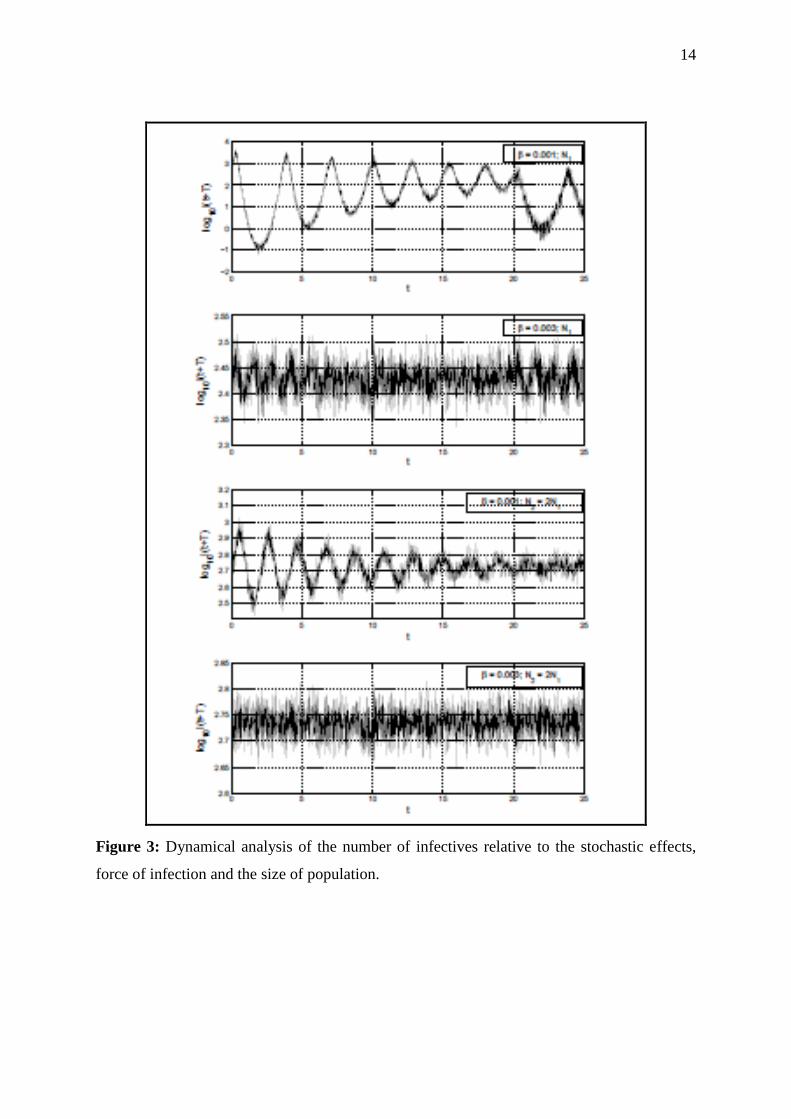
In figure 3, where the stochastic effects are effective, the change in the number of infectives
under the effects of (a) force of infection, (b) population size and (c) the stochastic effects are
plotted. This figure demonstrates clearly that time series has two main streams of oscillation;
smaller and higher for all the plots. It is diffcult to understand the dynamics for immense
population size with stronger force of infection i.e. as β increases from 0.001 to 0.003. Figure
4 presents the deterministic and stochastic analysis of S, E and I relative to time (transient
analysis). There are more fluctuations in stochastic model as compared to the deterministic
model. At the initial stage of infectious spread there are high oscillations and in the interval 10-
20 days there is damping. After passing 20 days, it seems that the infection dies out in
deterministic model but it still remains in the population which can be seen from the stochastic
modelling. Figure 5 depicts the orbital relation between the population of susceptible, exposed
and infectious. There is a twist in the portraits relative to change in size of population. We can
see that as the force of infection increases, the orbital span decreases, since the three sub-
populations are strongly correlated in that scenario. Precisely, for Na the infectives population
oscillates around 102.45 and around 102.75 for Nb. Figure 6 exhibits an interesting behavior for
the stochastic version of the S-E-I model. When we change the size of the population, there are
random distributions and the results are irregular. In the deterministic model, the orbital span
is not overlapping with the layers while in the stochastic model, evidently the orbital span is
jumbled. The orbital span increases in stochastic perturbations as compared to the deterministic
model relative to an increase in seasonality. We observe that random effects are more dominant
when the population is small and there is no twist in the phase space portraits when population
size is doubled. The solution converges to an equilibrium point as we increase the value of β
from 0.001 to 0.003 and the critical points are more precisely defined when β changes from
0.003 to 0.006.
5. CONCLUSIONS
Favourable climate factors are prerequisite to allow the expansion of disease spread observed
over the last four decades. Besides that, human factors, including growing global population,
urbanization, and socio-economic limitations on control measures contribute to the spread of

9
many of the epidemic diseases [31]. The basic SEIR model is first converted to the SEI model
and then the most suitable stochastic model is considered, based on two important aspects.
These are firstly the Lipschitz criteria and secondly the stability analysis of the model with
graphical analysis and phase space portraits. It is hoped that the proposed analysis and the
results will aid mathematical biologists in conducting research in different domains where
stochastic modelling is applicable [31-42]. Trends in current human settlement, together with
rapidly expanded urban areas, exploding population density, and limited socio-economic
resources, suggest that the human factors, in addition to climate factors are important
components in understanding current and future risks of disease transmission [1, 32].
Settlement and socio-economic factors together with climatic suitably, globalized travel and
trade, suggest that human populations and their collective actions strongly contribute to the
pandemic and epidemic diseases spread. The present study has shown that a deterministic
model oscillates in phase as compared to a stochastic model. Complex dynamical behaviour
has been reported in the seasonally forced spatial model along with the coexistence of perturbed
patterns. Chaotic solutions are observed for higher values of seasonal forcing. An important
conclusion from the present analysis is that it is necessary to consider not only the natural
structure and spread of the population but also the random effects. In this discussion we have
limited our analysis to forced perturbations. The size of population matters for both
deterministic and stochastic models. However from this extended model, we have demonstrated
that it may be essential to consider some important biological factors including heterogeneity,
stochasticity and geographic aspects. Future work, it is envisaged, will focus on the stochastic
analysis of delayed differential equations, where the delay will be based on the incubation
period. In this paper we discussed the stochastic analysis using the Euler-Maruyama method.
In subsequent investigations, it is feasible to deploy the s-stage diagonally implicit stochastic
Runge-Kutta methods (where s ≥ 2) with strong order for strong solutions. Such methods have
a large stability region. We will also consider hybrid stochastic Runge-Kutta methods which
are the combination of semi-implicit Runge-Kutta methods and implicit Runge-Kutta methods.
ACKNOWLEDGEMENTS
The authors are extremely grateful to both reviewers for their comments which have improved
the present work.
REFERENCES
[1] Vynnycky, E. and White, R., An Introduction to Infectious Disease Modeling
www.anintroductiontoinfectiousdiseasemodelling.com (2014).

10
[2] Alonso, David, Alan J. McKane, and Mercedes Pascual. Stochastic amplification in
epidemics, Journal of the Royal Society Interface 4.14 (2007): 575-582.
[3] Wilkinson, D. J., Stochastic Modelling for Systems Biology, CRC Press, Florida, USA
(2011).
[4] Liu, Zhenjie. Dynamics of positive solutions to SIR and SEIR epidemic models with
saturated incidence rates. Nonlinear Analysis: Real World Applications, 14.3 (2013): 1286-
1299.
[5] Altizer, S., Dobson, A., Hosseini, P., Hudson, P., Pascual, M. and Rohani, P., Seasonality
and the dynamics of infectious diseases. Ecology Letters, 9( 2006), 467-484.
[6] Naumova, E., Principles of Seasonality Assessment. Epidemiology, 19(2008), S49.
[7] Grassly, N. C. and Fraser, C. (2006). Seasonal infectious disease epidemiology. Proc. Royal
Society of London B: Biological Sciences, 273(1600), 2541-2550.
[8] Keeling, M. J., & Rohani, P.,. Modeling Infectious Diseases in Humans and Animals.
Princeton University Press, New Jersey, USA (2008).
[9] Fisman, D. N., Seasonality of infectious diseases, Ann. Rev. Public Health, 28 (2007) 127-
143.
[10] Read, Jonathan M., et al. Social mixing patterns in rural and urban areas of southern China.
Proc. Royal Society of London B: Biological Sciences 281.1785 (2014): 20140268.
[11] Riley, Steven et al., Five challenges for spatial epidemic models, Epidemics, 10 (2015):
68-71.
[12] R.M. Anderson, R.M. May, Population biology of infectious diseases I, Nature, 180
(1979) 361.
[13] R.M. May, R.M. Anderson, Population biology of infectious diseases II, Nature, 280
(1979) 455.
[14] Hethcote, Herbert W. The mathematics of infectious diseases. SIAM Review 42.4 (2000):
599-653.
[15] Kitsak, Maksim, et al. Identification of influential spreaders in complex networks. Nature
Physics, 6.11 (2010): 888-893.
[16] Carmi, Shai, et al. A model of Internet topology using k-shell decomposition. Proc.
National Academy of Sciences 104.27 (2007): 11150-11154.
[17] Lloyd, Alun L., and Robert M. May. Spatial heterogeneity in epidemic models. Journal
of Theoretical Biology 179.1 (1996): 1-11.
[18] Mollison, Denis. Dependence of epidemic and population velocities on basic parameters.
Mathematical Biosciences 107.2 (1991): 255-287.

11
[19] Van den Bosch, Frank, J. A. J. Metz, and O. Diekmann. The velocity of spatial population
expansion, Journal of Mathematical Biology 28.5 (1990): 529-565.
[20] Schmidt, W. P., Suzuki, M., Dinh Thiem, V., White, R. G., Tsuzuki, A., Yoshida, L. M.,
Ariyoshi, K. (2011). Population density, water supply, and the risk of dengue fever in Vietnam:
cohort study and spatial analysis. PLoS Medicine, 8(8), 1082.
[21] Okubo, Akira, and Smon A. Levin. Diffusion and Ecological Problems: Modern
Perspectives. Vol. 14. Springer Science & Business Media, 2013.
[22] Higham, Desmond J., An algorithmic introduction to numerical simulation of stochastic
diff erential equations. SIAM Review 43.3 (2001): 525-546.
[23] Dunbar, Steven R. Stochastic Processes and Advanced Mathematical Finance,
Department of Mathematics, University of Nebraska-Lincoln, USA, April (2016) .
[24] Allen, L. J., An Introduction to Stochastic Processes with Applications to Biology. CRC
Press, Florida, USA (2010).
[25] Carletti, M., Numerical solution of stochastic differential problems in the biosciences.
Journal of Computational and Applied Mathematics, 185 (2006) 422-440.
[26] Tidd, C. W., L. F. Olsen, and W. M. Schaffer, The case for chaos in childhood epidemics.
II. Predicting historical epidemics from mathematical models, Proc. Royal Society of London
B: Biological Sciences 254.1341 (1993): 257-273.
[27] http://www.who.int/csr/disease/en/.
[28] Swinburn, Boyd A., et al., The global obesity pandemic: shaped by global drivers and
local environments, The Lancet, 378.9793 (2011): 804-814.
[29] Gubler DJ, Reiter P, Ebi KL, Yap W, Nasci R, Patz JA. Climate variability and change in
the United States: potential impacts on vector- and rodent-borne diseases. Environ Health
Perspect, 109 (2001) Suppl 2: 223233.
[30] Astrom C, Rocklov J, Hales S, Beguin A, Louis V, Sauerborn R. Potential distribution of
dengue fever under scenarios of climate change and economic development. Ecohealth. 9
(2012):448454.
[31] Wilder-Smith A, Gubler DJ. Geographic expansion of dengue: the impact of international
travel. Med. Clin. N. Am. 92 (2008):13771390.
[32] Astrom C, Rocklov J, Hales S, Beguin A, Louis V, Sauerborn R. Potential distribution of
dengue fever under scenarios of climate change and economic development. Ecohealth. 9
(2012):448454.
[33] Perra, N., & Gonalves, B. Modeling and predicting human infectious diseases. In Social
Phenomena (pp. 59-83). Springer International Publishing (2015).

12
[34] Gautam, K., & Gautam, K., Study of Mathematical Modeling on Effect of Swine Flu.
International Journal of Research in Advance Engineering, 1 (2015), 1-6.
[35] Moneim, I. A., & Khalil, H. A. (2015). Modelling and simulation of the spread of HBV
disease with infectious Latent, Applied Mathematics, 6(5), 745.
[36] Liu, M., & Zhang, D. A dynamic logistics model for medical resources allocation in an
epidemic control with demand forecast updating. Journal of the Operational Research Society
(2016). doi:10.1057/jors.2015.105
[37] Prats, C., Montaola-Sales, C., Gilabert-Navarro, J. F. et al. (2015). Individual-based
modeling of tuberculosis in a user-friendly interface: understanding the epidemiological role
of population heterogeneity in a city, Frontiers in Microbiology, 6 (2015).
http://dx.doi.org/10.3389/fmicb.2015.01564
[38] Duku, C., Sparks, A. H., & Zwart, S. J., Spatial modelling of rice yield losses in Tanzania
due to bacterial leaf blight and leaf blast in a changing climate. Climatic Change, (2015) 1-15.
DOI: 10.1007/s10584-015-1580-2
[39] De Pinho, M. D. R., Kornienko, I., & Maurer, H. Optimal Control of a SEIR Model with
Mixed Constraints and L 1 Cost. In CONTROLO 2014- Proc. 11th Portuguese Conference on
Automatic Control (pp. 135-145). Springer International Publishing (2014).
[40] Kotyrba, M., Volna, E., & Bujok, P. (2015). Unconventional modelling of complex system
via cellular automata and differential evolution. Swarm and Evolutionary Computation, 25, 52-
62.
[41] Ibeas, A., de la Sen, M., Alonso-Quesada, S., & Zamani, I. (2015). Stability analysis and
observer design for discrete-time SEIR epidemic models. Advances in Diff erence Equations,
1 (2015) 1-21.
[42] Silal, S. P., Little, F., Barnes, K. I., & White, L. J. Sensitivity to model structure: a
comparison of compartmental models in epidemiology. Health Systems (2015) DOI:
10.1057/HS.2015.2

13
TABLES
Parameter N mD
(per year)
β
(per year per infective)
σD
(per year)
D
(per year)
range 106-107 0.01-0.04 0.0005-0.01 40-50 60-80
Table 1: Epidemic model parametric values
FIGURES
Figure 1: Schematic diagram of disease spread.
Figure 2: Periodic spread for N = Na (left panel) and (b) N = Nb (right panel).
𝑚𝐷𝑁 𝜆𝐷𝑆 𝜎𝐷 𝐸 I E S
14
Figure 3: Dynamical analysis of the number of infectives relative to the stochastic effects,
force of infection and the size of population.

15
Figure 4: Transient analysis of the deterministic model (left panel) and stochastic model (right
panel) S, E and I.

16
Figure 5: Phase space portraits of S, E and I for deterministic model.

17

18
Figure 6: Phase space portraits of S, E and I for stochastic model.


