
Stress-Strain-Diffusion
Interactions in Solids
J. Svoboda1 and F.D. Fischer2
1Institute of Physics of Materials, Brno,Czech Republic
2Institute of Mechanics, Montanuniversität Leoben, Austria
DSL 2014
CONTENT
1. Introduction
2. Generalized Manning theory for diffusion
3. Solution of 1-D example – two assembled sheets
4. Simulation of system evolution
5. Summary/conclusions
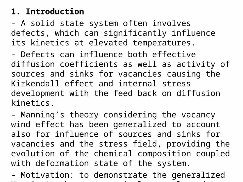
1. Introduction
- A solid state system often involves defects, which can significantly influence its kinetics at elevated temperatures. - Defects can influence both effective diffusion coefficients as well as activity of sources and sinks for vacancies causing the Kirkendall effect and internal stress development with the feed back on diffusion kinetics. - Manning’s theory considering the vacancy wind effect has been generalized to account also for influence of sources and sinks for vacancies and the stress field, providing the evolution of the chemical composition coupled with deformation state of the system.- Motivation: to demonstrate the generalized Manning’s theory on a simple example and to show the influence of stress-strain-diffusion interactions on the system evolution kinetics.
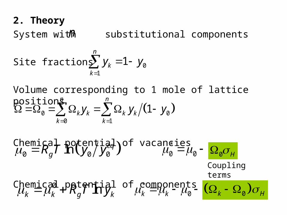
2. Theory
System with substitutional components
Site fractions
Volume corresponding to 1 mole of lattice positions
Chemical potential of vacancies
Chemical potential of components
01
1n
kk
y y
0 00 1
1n n
k k k kk k
y y y
0 0 0ln eqgR T y y
0 lnk k g kR T y
*0 0
*0k k
n
0 HCoupling terms
0k H
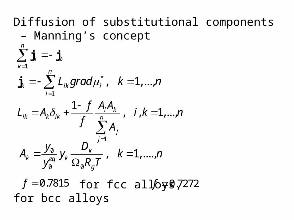
Diffusion of substitutional components – Manning’s concept
for fcc alloys, for bcc alloys
01
n
kk
j j
*
1
, 1,...,n
k ik ii
L grad k n
j
1
1, , 1,...,i k
ik k ik n
jj
f A AL A i k n
f A
0
0 0
, 1,....,kk keq
g
y DA y k n
y R T
0.7815f 0.7272f

Conservation laws
Generation/annihilation of vacancies at non-ideal sources/sinks
Generalized creep (Fischer, Svoboda: Int. J. Plasticity 27, 1384-1390, 2011)
0 , 1,...,k k ky y k n j
0 0 0 01
1n
kk
y y y
j
*0
bvK
0
0 02
eqg
bv
fy R TK
y DaH
1
1 1
1n n
ii i
i ii
yD f f y D
D
H I s
*0
010 0
2
3 15 3 1
ncr
k kkbv bvK K y
I
I j s

3. Solution of 1-D example – two assembled sheets
Interface at
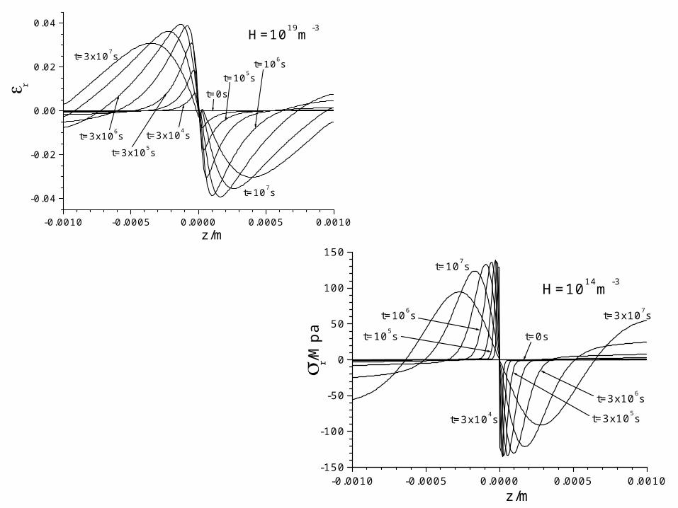
Axial (z-axis) symmetry
Elastic strain components
Creep strain rate components
Total strain components
0z 1 2h z h r z z 0z
2 3H r 3r rs s 2 3z rs
1 , 2el elr r z rv E z v E z
el crr r r el cr
z z z
,0
10
2 1
3 45 3 1
nk zcr r
r kkbv
j
K y z
,0
10
4 1
3 45 3 1
nk zcr r
z kkbv
j
K y z
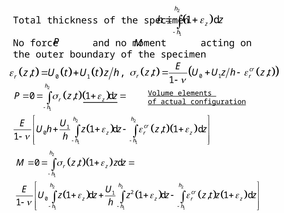
Total thickness of the specimen
No force and no moment acting on the outer boundary of the specimen
2
1
1 dh
z
h
h z
0 1, ,r z t U t U t z h 0 1, ,1
crr r
Ez t U U z h z t
2
1
2 2
1 1
10
0 , 1 d
1 d , 1 d1
h
r z
h
h hcr
z r z
h h
P z t z
UEU h z z z t z
h
2
1
2 2 2
1 1 1
210
0 , 1 d
1 d 1 d , 1 d1
h
r z
h
h h hcr
z z r z
h h h
M z t z z
UEU z z z z z t z z
h
P M
Volume elements of actual configuration________
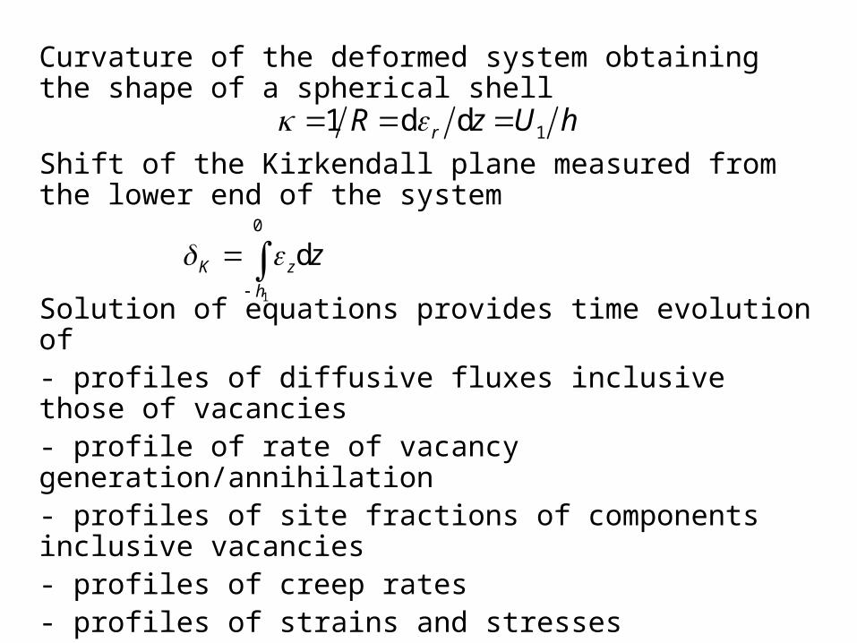
Curvature of the deformed system obtaining the shape of a spherical shell
Shift of the Kirkendall plane measured from the lower end of the system
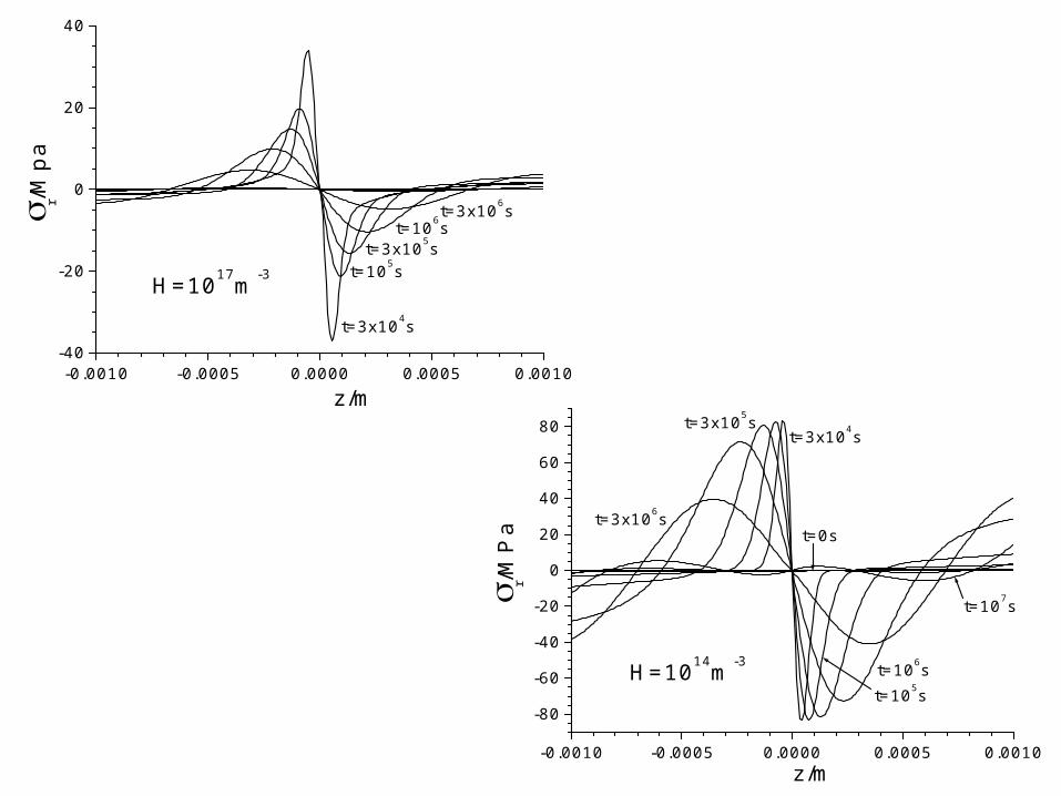
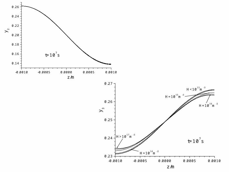
Solution of equations provides time evolution of- profiles of diffusive fluxes inclusive those of vacancies- profile of rate of vacancy generation/annihilation - profiles of site fractions of components inclusive vacancies- profiles of creep rates - profiles of strains and stresses- Kirkendall shift and curvature
11 d drR z U h
1
0
dK z
h
z
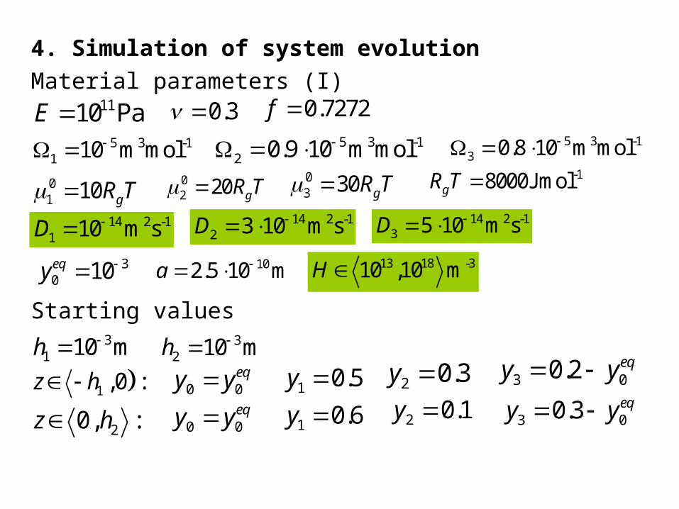
4. Simulation of system evolution
Material parameters (I)
Starting values
1110 PaE 0.3 0.7272f
30 10eqy
31 10 mh 3
2 10 mh
5 3 -11 10 m mol 5 3 -1
2 0.9 10 m mol 5 3 -13 0.8 10 m mol
01 10 gR T
-18000JmolgR T 02 20 gR T 0
3 30 gR T 14 2 -1
1 10 m sD 14 2 -12 3 10 m sD 14 2 -1
3 5 10 m sD
102.5 10 ma 13 18 -310 ,10 mH
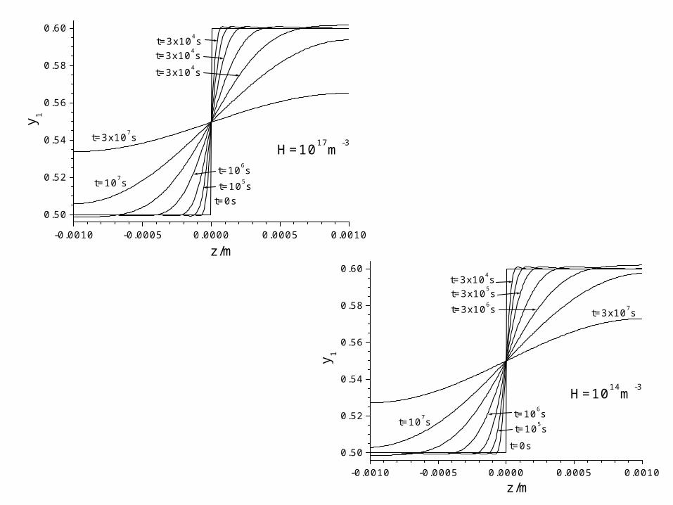
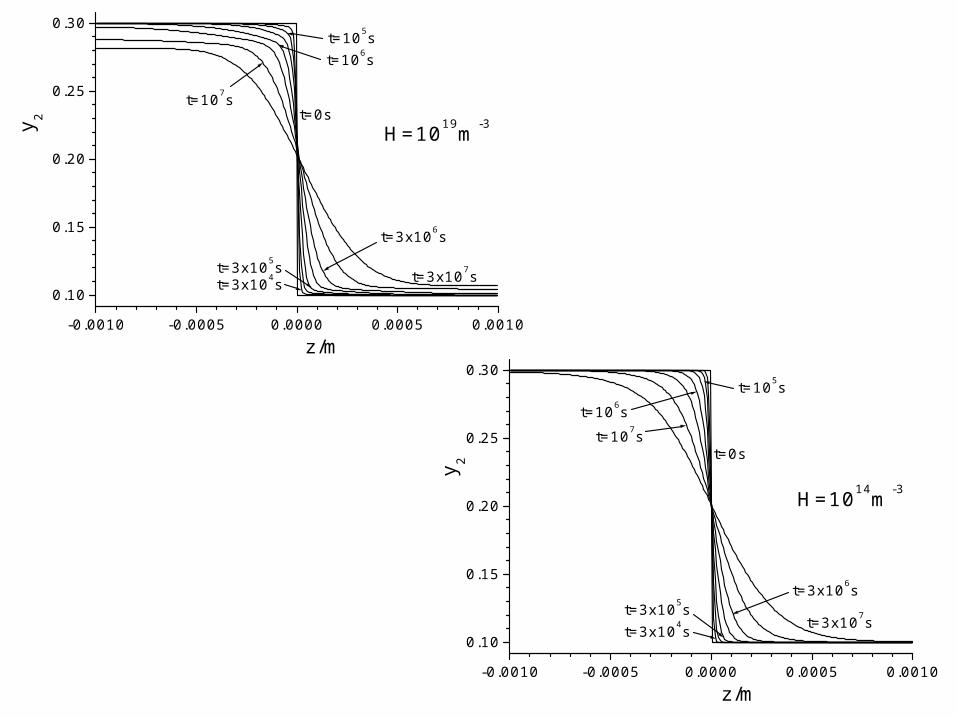
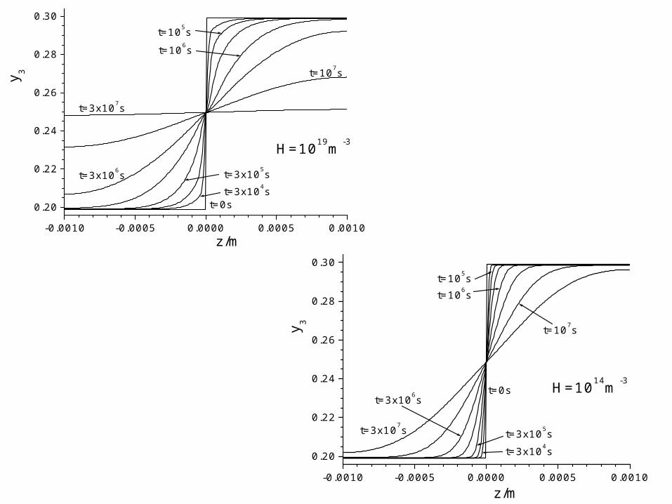
1 ,0 :z h 0 0eqy y 1 0.5y 2 0.3y 3 00.2 eqy y
20, :z h 0 0eqy y 1 0.6y 3 00.3 eqy y 2 0.1y
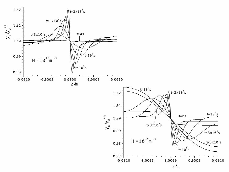
-0.0010 -0.0005 0.0000 0.0005 0.0010
0.98
0.99
1.00
1.01
1.02
H=1017m-3
t=0s
t=105s
t=106s
t=3x10⁴s
t=3x10⁴s
t=3x10⁴sy 0/
y 0eq
z/m
-0.0010 -0.0005 0.0000 0.0005 0.00100.97
0.98
0.99
1.00
1.01
1.02
H=1014m-3
t=3x10⁵s
t=106s
t=107s
t=3x10⁷s
t=0s
t=3x10⁶s
t=3x10⁴s
t=105s
y 0/y 0eq
z/m
-0.0010 -0.0005 0.0000 0.0005 0.0010
0.50
0.52
0.54
0.56
0.58
0.60
H=1017m-3
t=3x10⁴s
t=3x10⁷s
t=3x10⁴s
t=3x10⁴s
t=107st=106st=105s
t=0s
y 1
z/m
-0.0010 -0.0005 0.0000 0.0005 0.0010
0.50
0.52
0.54
0.56
0.58
0.60
H=1014m-3
t=3x10⁴st=3x10⁵st=3x10⁶s t=3x10⁷s
t=107st=106st=105s
t=0s
y 1
z/m

-0.0010 -0.0005 0.0000 0.0005 0.0010
0.10
0.15
0.20
0.25
0.30
H=1017m-3t=105s
t=3x10⁵s
t=3x10⁴s
t=107s
t=3x10⁶s
t=3x10⁷s
t=106s
t=0sy 2
z/m
-0.0010 -0.0005 0.0000 0.0005 0.0010
0.10
0.15
0.20
0.25
0.30
H=1014m-3t=107s
t=106s
t=105s
t=0s
t=3x10⁶s
t=3x10⁷s
t=3x10⁵s
t=3x10⁴s
y 2
z/m

-0.0010 -0.0005 0.0000 0.0005 0.0010
0.20
0.22
0.24
0.26
0.28
0.30
H=1017m-3
t=0s
t=105s
t=3x10⁵s
t=106s
t=3x10⁶s
t=107s
t=3x10⁷s
t=3x10⁴s
y 3
z/m
-0.0010 -0.0005 0.0000 0.0005 0.0010
0.20
0.22
0.24
0.26
0.28
0.30
H=1014m-3
t=3x10⁷s
t=3x10⁵s t=3x10⁶s
t=3x10⁴s
t=107s
t=106s
t=105s
t=0s
y 3
z/m
-0.0010 -0.0005 0.0000 0.0005 0.0010
-80
-60
-40
-20
0
20
40
60
80
H=1014m-3
t=107s
t=105st=106s
t=0st=3x10⁶s
t=3x10⁵st=3x10⁴s
r/MP
a
z/m
-0.0010 -0.0005 0.0000 0.0005 0.0010-40
-20
0
20
40
H=1017m-3
t=3x10⁶st=106s
t=3x10⁵st=105s
t=3x10⁴s
r/Mpa
z/m

-0.0010 -0.0005 0.0000 0.0005 0.00100.97
0.98
0.99
1.00
1.01
1.02
1.03
H=1017m-3
H=1018m-3H=1016m-3
H=1015m-3
H=1014m-3
H=1013m-3
t=107s
y 0/y 0e
q
z/m
-0.0010 -0.0005 0.0000 0.0005 0.00100.50
0.52
0.54
0.56
0.58
0.60
H<1014m-3
H>1016m-3
H=1015m-3
t=107s
y 1
z/m
-0.0010 -0.0005 0.0000 0.0005 0.0010
0.14
0.16
0.18
0.20
0.22
0.24
0.26
t=107s
y 2
z/m
-0.0010 -0.0005 0.0000 0.0005 0.00100.23
0.24
0.25
0.26
0.27
H=1015m-3
H=1016m-3
H>1017m-3
H=1014m-3
H<1013m-3
t=107s
y 3
z/m
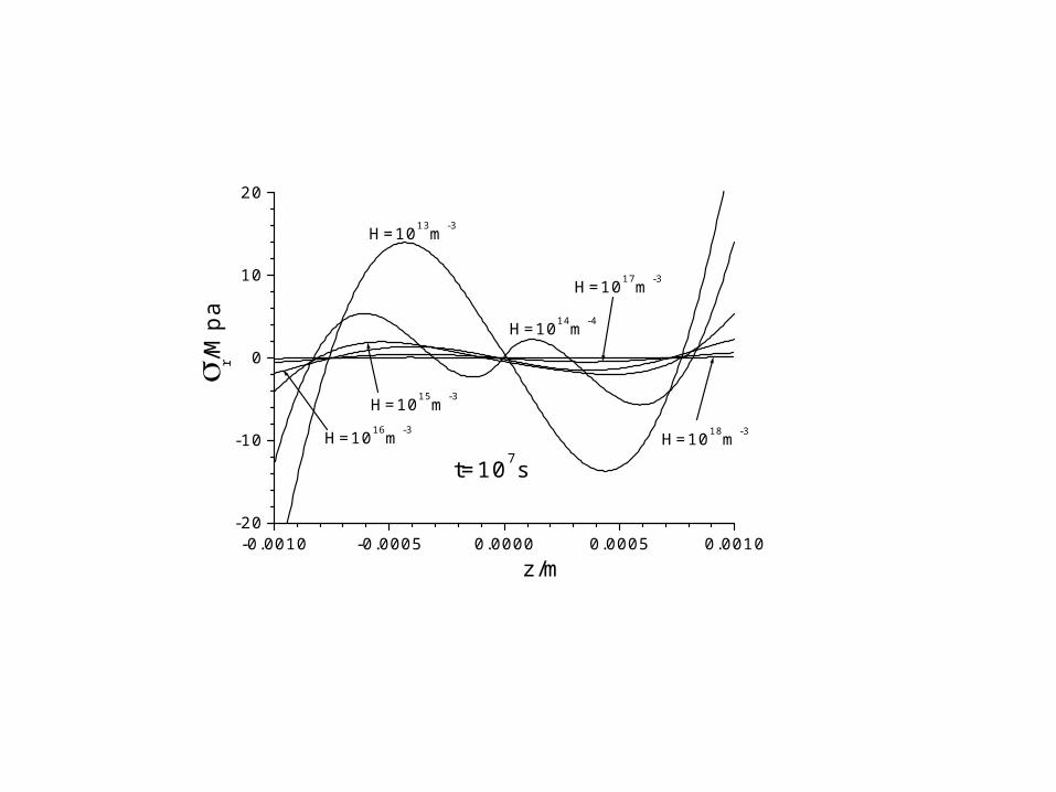
-0.0010 -0.0005 0.0000 0.0005 0.0010-20
-10
0
10
20
t=107sH=1018m-3
H=1017m-3
H=1016m-3
H=1015m-3
H=1014m-4
H=1013m-3 r/M
pa
z/m
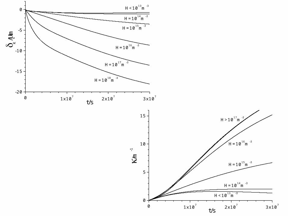
0 1x10⁷ 2x10⁷ 3x10⁷-20
-15
-10
-5
0
H=1018m-3
H=1017m-3
H=1016m-3
H=1015m-3
H=1014m-3
H<1013m-3
K/
m
t/s
0 1x10⁷ 2x10⁷ 3x1070
5
10
15H>1017m-3
H=1016m-3
H=1015m-3
H=1014m-3
H<1013m-3
/m-1
t/s
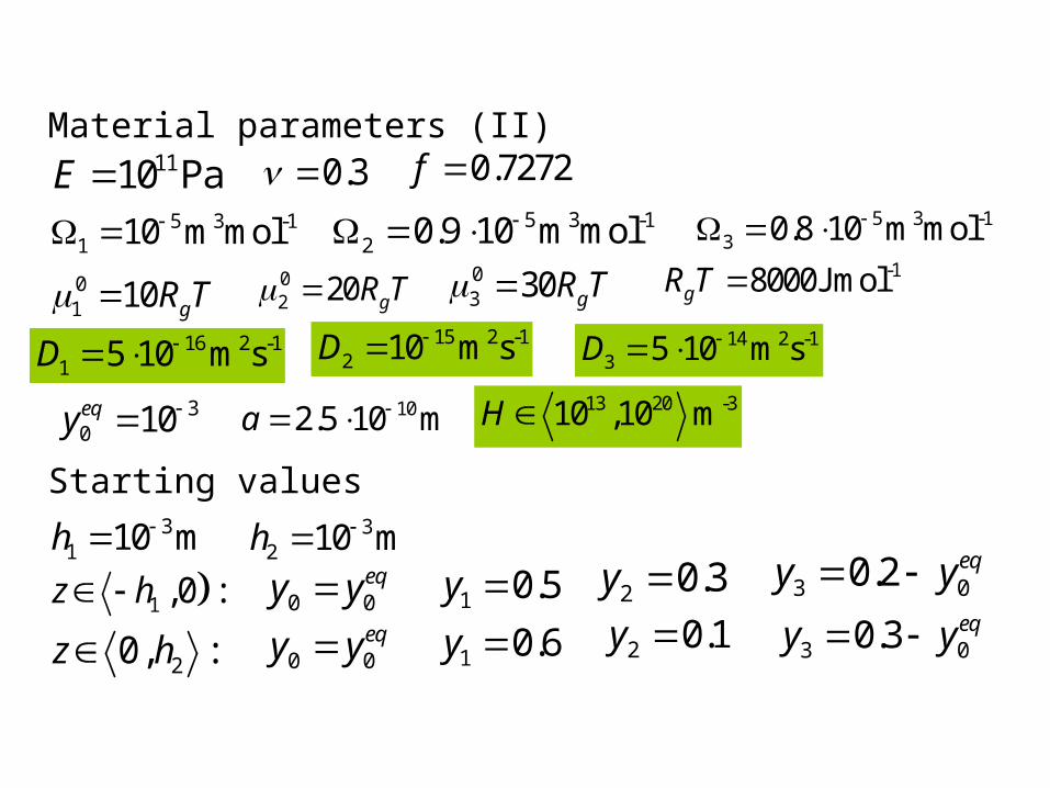
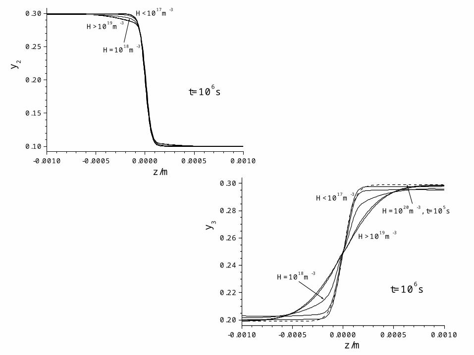
Material parameters (II)
Starting values
1110 PaE 0.3 0.7272f
30 10eqy
31 10 mh 3
2 10 mh
5 3 -11 10 m mol 5 3 -1
2 0.9 10 m mol 5 3 -13 0.8 10 m mol
01 10 gR T
-18000JmolgR T 02 20 gR T 0
3 30 gR T 16 2 -1
1 5 10 m sD 15 2 -1
2 10 m sD 14 2 -13 5 10 m sD
102.5 10 ma 13 20 -310 ,10 mH
1 ,0 :z h 0 0eqy y 1 0.5y 2 0.3y 3 00.2 eqy y
20, :z h 0 0eqy y 1 0.6y 3 00.3 eqy y 2 0.1y

-0.0010 -0.0005 0.0000 0.0005 0.0010
0.90
0.95
1.00
1.05
1.10
H=1019m-3
t=106s
t=105s
t=0s, t>107s
t=3x10⁶st=3x10⁵s
t=3x10⁴sy 0/
y 0eq
z/m
-0.0010 -0.0005 0.0000 0.0005 0.00100.8
0.9
1.0
1.1
1.2
H=1014m-3
t=3x10⁵s
t=3x10⁶s t=3x10⁴s
t=105s
t=106st=107s
t=0s
t=3x10⁷sy 0/
y 0eq
z/m
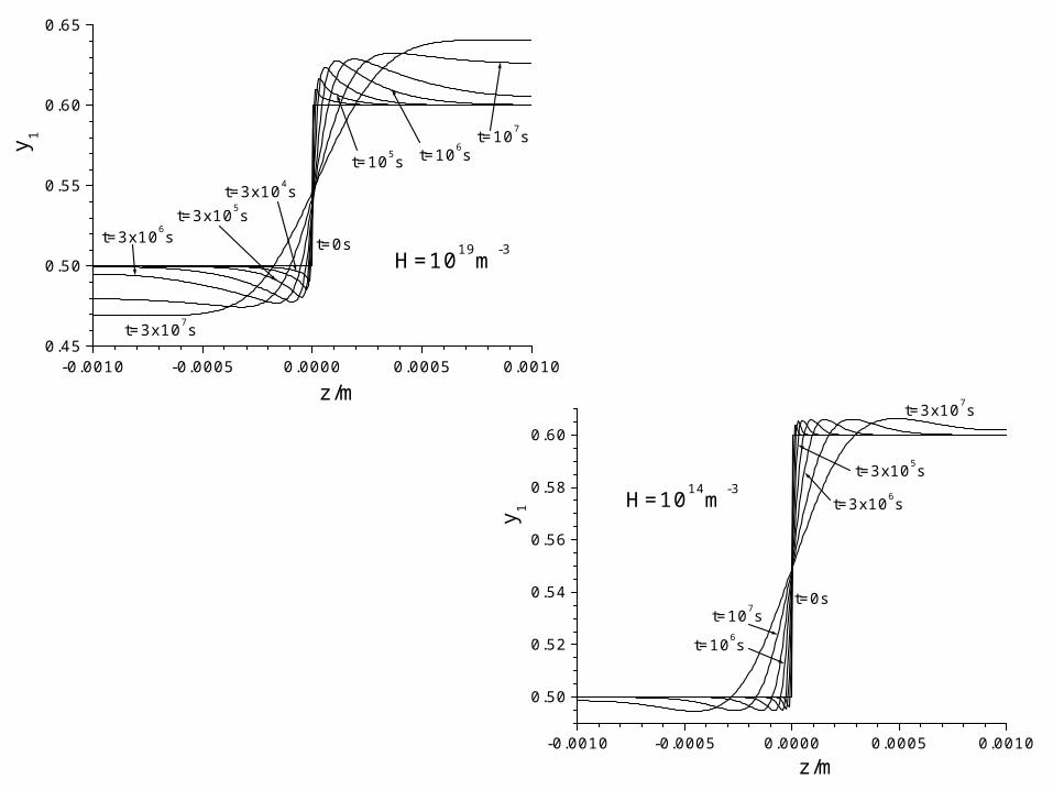
-0.0010 -0.0005 0.0000 0.0005 0.0010
0.50
0.52
0.54
0.56
0.58
0.60
t=0s
H=1014m-3
t=106s
t=107s
t=3x10⁶s
t=3x10⁵s
t=3x10⁷s
y 1
z/m
-0.0010 -0.0005 0.0000 0.0005 0.00100.45
0.50
0.55
0.60
0.65
H=1019m-3
t=3x10⁴st=3x10⁵s
t=3x10⁶s
t=3x10⁷s
t=0s
t=105s t=106st=107sy 1
z/m
-0.0010 -0.0005 0.0000 0.0005 0.0010
0.10
0.15
0.20
0.25
0.30
H=1019m-3
t=107s
t=106st=105s
t=3x10⁵st=3x10⁴s
t=0s
t=3x10⁶s
t=3x10⁷s
y 2
z/m
-0.0010 -0.0005 0.0000 0.0005 0.0010
0.10
0.15
0.20
0.25
0.30
H=1014m-3
t=3x10⁴st=3x10⁵s
t=3x10⁶s
t=0s
t=105s
t=106s
t=3x10⁷s
t=107sy 2
z/m
-0.0010 -0.0005 0.0000 0.0005 0.0010
0.20
0.22
0.24
0.26
0.28
0.30
H=1014m-3t=0s
t=105s
t=107s
t=106s
t=3x10⁵s
t=3x10⁴s
t=3x10⁷s
t=3x10⁶s
y 3
z/m
-0.0010 -0.0005 0.0000 0.0005 0.0010
0.20
0.22
0.24
0.26
0.28
0.30
H=1019m-3
t=105s
t=106s
t=107s
t=0st=3x10⁴s
t=3x10⁵st=3x10⁶s
t=3x10⁷s
y 3
z/m
-0.0010 -0.0005 0.0000 0.0005 0.0010
-0.04
-0.02
0.00
0.02
0.04H=1019m-3
t=3x10⁴s
t=3x10⁵s
t=105st=0s
t=106s
t=3x10⁶s
t=3x10⁷s
t=107s
r
z/m
-0.0010 -0.0005 0.0000 0.0005 0.0010-150
-100
-50
0
50
100
150
H=1014m-3
t=3x10⁴s t=3x10⁵s
t=3x10⁶s
t=105s
t=3x10⁷s
t=0s
t=107s
t=106s r/M
pa
z/m
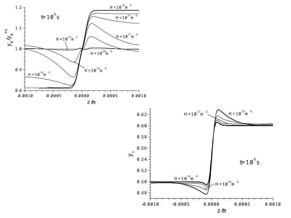
-0.0010 -0.0005 0.0000 0.0005 0.00100.8
0.9
1.0
1.1
1.2
H=1019m-3
H=1018m-3
H=1017m-3
H=1016m-3
H=1015m-3
H=1020m-3
H<1014m-3
t=106sy 0/
y 0eq
z/m
-0.0010 -0.0005 0.0000 0.0005 0.0010
0.48
0.50
0.52
0.54
0.56
0.58
0.60
0.62
t=106s
H=1016m-3
H=1017m-3
H=1018m-3
H>1019m-3
y 1
z/m
-0.0010 -0.0005 0.0000 0.0005 0.0010
0.10
0.15
0.20
0.25
0.30
t=106s
H=1018m-3
H>1019m-3
H<1017m-3y 2
z/m
-0.0010 -0.0005 0.0000 0.0005 0.0010
0.20
0.22
0.24
0.26
0.28
0.30
H=1020m-3, t=105s
H=1018m-3
H<1017m-3
H>1019m-3
t=106s
y 3
z/m
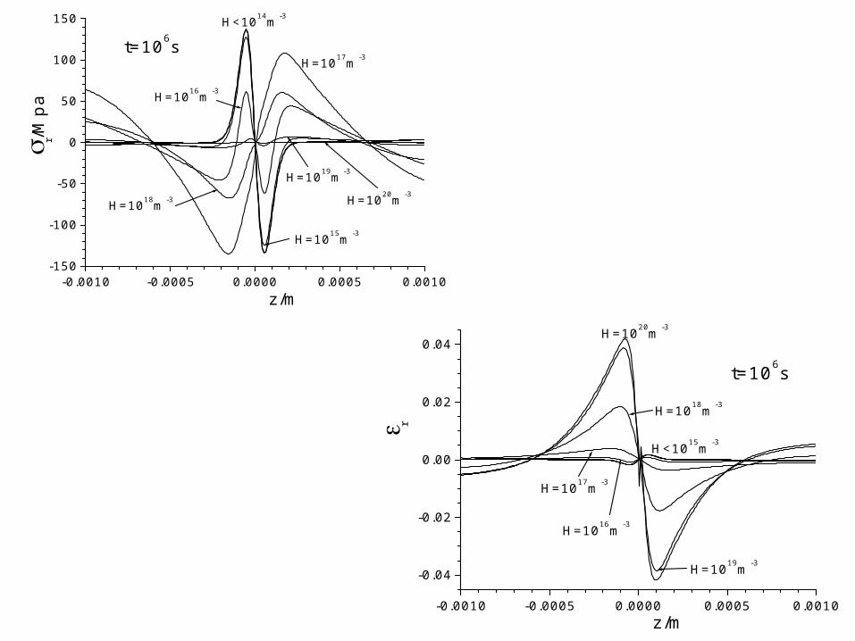
-0.0010 -0.0005 0.0000 0.0005 0.0010-150
-100
-50
0
50
100
150
t=106s
H=1020m-3
H=1019m-3
H=1017m-3
H=1018m-3
H=1016m-3
H=1015m-3
H<1014m-3
r/Mpa
z/m
-0.0010 -0.0005 0.0000 0.0005 0.0010
-0.04
-0.02
0.00
0.02
0.04
t=106s
H<1015m-3
H=1016m-3
H=1017m-3
H=1019m-3
H=1018m-3
H=1020m-3
r
z/m
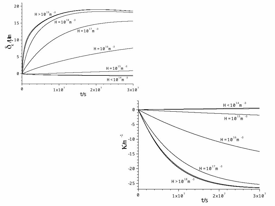
0 1x10⁷ 2x10⁷ 3x10⁷
0
5
10
15
20
H>1019m-3
H=1018m-3
H=1017m-3
H=1016m-3
H<1014m-3
H=1015m-3
K/
m
t/s
0 1x10⁷ 2x10⁷ 3x10⁷
-25
-20
-15
-10
-5
0H<1014m-3
H>1018m-3
H=1017m-3
H=1016m-3
H=1015m-3
/m-1
t/s

5. Summary/conclusions- Generalized Manning theory for diffusion of substitutional
components accounting for sources and sinks for vacancies and interaction with developing internal stress field are presented.
- The theory is demonstrated on simulation of evolution of a diffusion couple consisting of two assembled sheets; activity of sources and sinks for vacancies and diffusion coefficients are taken as system parameters.
- For nearly the same diffusion coefficients of all components the influence of activity of sources and sinks for vacancies on system evolution kinetics is not significant.
- For significantly different diffusion coefficients the influence of activity of sources and sinks for vacancies is evident. In such a case the measurement of diffusion coefficients MUST be completed by the characterization of the microstructure! If this is NOT done, the measured diffusion coefficients loose their credibility.


