

Brigham Young University Brigham Young University
BYU ScholarsArchive BYU ScholarsArchive
Theses and Dissertations
2006-12-21
Structuring Emperical Methods for Reuse and Efficiency in Structuring Emperical Methods for Reuse and Efficiency in
Product Development Processes Product Development Processes
Marshall Edwin Bare Brigham Young University - Provo
Follow this and additional works at: https://scholarsarchive.byu.edu/etd
Part of the Mechanical Engineering Commons
BYU ScholarsArchive Citation BYU ScholarsArchive Citation Bare, Marshall Edwin, "Structuring Emperical Methods for Reuse and Efficiency in Product Development Processes" (2006). Theses and Dissertations. 1032. https://scholarsarchive.byu.edu/etd/1032
This Thesis is brought to you for free and open access by BYU ScholarsArchive. It has been accepted for inclusion in Theses and Dissertations by an authorized administrator of BYU ScholarsArchive. For more information, please contact [email protected], [email protected].

STRUCTURING EMPIRICAL METHODS FOR REUSE AND
EFFICIENCY IN PRODUCT DEVELOPMENT PROCESSES
by
Marshall Edwin Bare
A thesis submitted to the faculty of
Brigham Young University
in partial fulfillment of the requirements for the degree of
Master of Science
Department of Mechanical Engineering
Brigham Young University
April 2007


BRIGHAM YOUNG UNIVERSITY
GRADUATE COMMITTEE APPROVAL
of a thesis submitted by
Marshall Edwin Bare This thesis has been read by each member of the following graduate committee and by majority vote has been found to be satisfactory. Date Jordan J. Cox, Chair
Date Jeffrey P. Bons
Date Brian D. Jensen


BRIGHAM YOUNG UNIVERSITY As chair of the candidate’s graduate committee, I have read the thesis of Marshall Edwin Bare in its final form and have found that (1) its format, citations, and bibliographical style are consistent and acceptable and fulfill university and department style requirements; (2) its illustrative materials including figures, tables, and charts are in place; and (3) the final manuscript is satisfactory to the graduate committee and is ready for submission to the university library. Date Jordan J. Cox
Chair, Graduate Committee
Accepted for the Department
Matthew R. Jones Graduate Coordinator
Accepted for the College
Alan R. Parkinson Dean, Ira A. Fulton College of Engineering and Technology


ABSTRACT
STRUCTURING EMPIRICAL METHODS FOR REUSE AND
EFFICIENCY IN PRODUCT DEVELOPMENT PROCESSES
Marshall Bare
Department of Mechanical Engineering
Master of Science Product development requires that engineers have the ability to predict product
performance. When product performance involves complex physics and natural
phenomena, mathematical models are often insufficient to provide accurate predictions.
Engineering companies compensate for this deficiency by testing prototypes to obtain
empirical data that can be used in place of predictive models. The purpose of this work is
to provide techniques and methods for efficient use of empirical methods in product
development processes.
Empirical methods involve the design and creation of prototype hardware and the
testing of that hardware in controlled environments. Empirical methods represent a
complete product development sub-cycle within the overall product development process.
Empirical product development cycles can be expensive in both time and resources.


Global economic pressures have caused companies to focus on improving the
productivity of their product development cycles. A variety of techniques for improving
the productivity of product development processes have been developed. These methods
focus on structuring process steps and product artifacts for reuse and efficiency.
However these methods have, to this point, largely ignored the product development sub-
cycle of empirical design. The same techniques used on the overall product development
processes can and should be applied to the empirical product development sub-cycle.
This thesis focuses on applying methods of efficient and reusable product
development processes on the empirical development sub-cycle. It also identifies how to
efficiently link the empirical product development sub-cycle into the overall product
development process. Specifically, empirical product development sub-cycles can be
characterized by their purposes into three specific types: first, obtaining data for
predictive model coefficients, boundary conditions and driving functions; second,
validating an existing predictive model; and third, to provide the basis for predictions
using interpolation and extrapolation of the empirical data when a predictive model does
not exist. These three types of sub-cycles are structured as reusable processes in a
standard form that can be used generally in product development. The roles of these
three types of sub-cycles in the overall product development process are also established
and the linkages defined. Finally, the techniques and methods provided for improving
the efficiency of empirical methods in product development processes are demonstrated
in a form that shows their benefits.


ACKNOWLEDGEMENTS
I thank God for all His help in getting me to this point in my life. I also thank my
wife, Mandy, for her patience and support. Finally, I thank Dr. Cox for his willingness to
take me under his wing. His untiring help, support, and friendship have given me insight
on what it means to be a Christian.


TABLE OF CONTENTS
Chapter 1. Introduction.......................................................................................................1
Defining The Problem..................................................................................................... 1
Thesis Statement ............................................................................................................. 3
Chapter 2. Background & Literature Review .....................................................................5
Improving Product Development.................................................................................... 5
Improving Empirical Methods........................................................................................ 6
Reuse Not a Major Consideration in Today’s Methods.................................................. 7
Chapter 3. Method ............................................................................................................11
Roles of Empirical Product Development .................................................................... 11
Typical Design Process................................................................................................. 12
Typical Detailed Design Phase Including Empirical Processes ................................... 13
Current Typical Empirical Processes............................................................................ 15
A Modern Technique for Reorganizing the Detailed Design and Testing Processes... 22
Organizing the Empirical Process into Reusable Steps ................................................ 27
Integrating the Empirical Process into the Product Design Map.................................. 31
Chapter 4. Test Cases .......................................................................................................35
Case 1 – Aspirator – A predictive model needs to be completed or updated ............... 36
1st Iteration, Traditional Approach............................................................................ 46
2nd Iteration, Traditional Approach........................................................................... 48
xiii
1st Iteration, PDG Approach ..................................................................................... 50
2nd Iteration, PDG Approach..................................................................................... 52
Case 2 – Aspirator – A predictive model must be validated......................................... 54
1st Iteration, Traditional Approach............................................................................ 64
2nd Iteration, Traditional Approach........................................................................... 65
1st Iteration, PDG Approach ..................................................................................... 67
2nd Iteration, PDG Approach..................................................................................... 68
Case 3 – Daisy Mixer – A predictive model does not exist.......................................... 70
Comparison of Traditional Method Vs. Proposed Method....................................... 80
1st Iteration, Traditional Approach:........................................................................... 82
2nd Iteration, Traditional Approach:.......................................................................... 84
1st Iteration, PDG approach....................................................................................... 86
2nd Iteration, PDG approach...................................................................................... 89
Chapter 5. Implementation of PDG Approach .................................................................93
Chapter 6. Results and Conclusions ...............................................................................102
References........................................................................................................................106
Appendix..........................................................................................................................109
xiv

LIST OF FIGURES
Figure 1. NASA “stage gate” Product Development Process........................................... 13
Figure 2. Virtual Prediction .............................................................................................. 14
Figure 3. Detailed Design Phase....................................................................................... 15
Figure 4. Typical Empirical Process Model ..................................................................... 16
Figure 5. Product Design Generator (PDG) Sets and Maps ............................................. 24
Figure 6. Sample Process Map of Constant Force Spring ................................................ 26
Figure 7. PDG Structure Applied to the Empirical Process............................................. 28
Figure 8. Empirical Process PDG Integrated into Main PDG ......................................... 31
Figure 9. Empirical Process Used to Complete or Update Predictive Model.................. 32
Figure 10. Empirical Process Used in Place of Predictive Model ................................... 33
Figure 11. Empirical Process Used to Validate Predictive Model................................... 34
Figure 12. CAD Model of Simple Aspirator Design ....................................................... 37
Figure 13. Empirical Process Used to Complete or Update Predictive Model................ 46
Figure 14. Breathing Cycle Without Aspirator................................................................ 55
Figure 15. Typical Aspirator Screen Performance .......................................................... 57
Figure 16. Process Used to Validate Predictive Model ................................................... 63
Figure 17. Aspirator Tube Showing Cross-Section, Traditional Approach..................... 65
Figure 18. Aspirator Tube Showing Cross-Section, PDG Approach .............................. 68
Figure 19. Prototype Design Involves Complete Design Process ................................... 71
xv

Figure 20. Daisy Mixer General Set-up........................................................................... 72
Figure 21. PIV Cameras................................................................................................... 73
Figure 22. PIV Laser Sheet.............................................................................................. 73
Figure 23. Empirical Process Used in Place of Predictive Model ................................... 78
Figure 24. Daisy Mixer Backwards Map 1...................................................................... 94
Figure 25. Daisy Mixer Backwards Map 2...................................................................... 95
Figure 26. Detailed Map of Daisy Mixer Design Process ............................................... 97
Figure 27. Daisy Mixer Maps & Sets Schematic............................................................. 99
Figure 28. Daisy Mixer Parameter List Sample............................................................. 100
Figure A1. PIV Documentation Slide 1.......................................................................... 110
Figure A2. PIV Documentation Slide 2.......................................................................... 111
Figure A3. PIV Documentation Slide 3.......................................................................... 112
Figure A4. PIV Documentation Slide 4.......................................................................... 113
Figure A5. PIV Documentation Slide 5.......................................................................... 114
Figure A6. PIV Documentation Slide 6.......................................................................... 115
Figure A7. PIV Documentation Slide 7.......................................................................... 116
Figure A8. PIV Documentation Slide 8.......................................................................... 117
Figure A9. PIV Documentation Slide 9.......................................................................... 118
Figure A10. PIV Documentation Slide 10...................................................................... 119
Figure A11. PIV Documentation Slide 11...................................................................... 120
Figure A12. PIV Documentation Slide 12...................................................................... 121
Figure A13. PIV Documentation Slide 13...................................................................... 122
Figure A14. PIV Documentation Slide 14...................................................................... 123
xvi

Figure A15. PIV Documentation Slide 15...................................................................... 124
Figure A16. PIV Documentation Slide 16...................................................................... 125
Figure A17. PIV Documentation Slide 17...................................................................... 126
Figure A18. PIV Documentation Slide 18...................................................................... 127
Figure A19. PIV Documentation Slide 19...................................................................... 128
Figure A20. PIV Documentation Slide 20...................................................................... 129
Figure A21. PIV Documentation Slide 21...................................................................... 130
Figure A22. PIV Documentation Slide 22...................................................................... 131
Figure A23. PIV Documentation Slide 23...................................................................... 132
Figure A24. PIV Documentation Slide 24...................................................................... 133
Figure A25. PIV Documentation Slide 25...................................................................... 134
xvii

xviii

LIST OF TABLES
Table 1. Example of Empirical Process Sets and Maps................................................... 29
xix

xx

Chapter 1. Introduction
Defining The Problem
Product development requires that engineers have the ability to predict product
performance. When product performance involves complex physics and natural
phenomena, mathematical models are often insufficient to provide accurate predictions.
“If the underlying physics of a product is not well understood, analytical estimates cannot
be expected to produce accurate results.” 1 Engineering companies compensate for this
deficiency by testing prototypes to obtain empirical data that can be used in place of
predictive models. Even considering modern advances in engineering modeling and
predictive software, prototypes are viewed as indispensable by today’s leading
companies. Ullman2 reports on Toyota’s dependence on prototypes and the benefit of
having hard facts in front of the engineers. “Toyota has resisted [computer modeling]
technologies in favor of developing physical prototypes, especially in the design of
components that are primarily visual (e.g., car bodies). In fact, Toyota claims that
through the use of many simple prototypes, it can develop cars with fewer people and less
time than companies that rely heavily on computers. The number of prototypes to
schedule is dependent on the company culture and the ability to produce usable
prototypes rapidly.” David Packer of Hewlett-Packard comments on the need for
prototypes, “There is only one road to reliability. Build it, test it, and fix the things that
go wrong. Repeat the process until the desired reliability is achieved.” 3 Considering the
necessity of empirical methods, the purpose of this work is to provide techniques and
1

methods to increase the efficiency of modern empirical methods in product development
processes.
Empirical methods involve the design and creation of prototype hardware and the
testing of that hardware in controlled environments. Empirical methods represent a
complete product development sub-cycle within the overall product development process.
Empirical product development cycles can be expensive in both time and resources.
Doebelin3 notes, “Although good first-round designs are an essential foundation, the bulk
of the engineer’s efforts go into executing well-thought-out testing programs whose
intent is to stress the design and uncover its limitations so that improvements in the
subsystems and the integrated product can be made… We often find that testing efforts
comprise more than half of the entire engineering effort.” Even in reverse engineering,
the “building and testing of prototypes often constitutes a large portion of the cost to
reverse engineer a part.”4 While many understand the need to increase the efficiency of
empirical processes, a broader and longer term perspective on the purpose of prototypes
would provide for better planning of the elements of empirical processes. “One company
had a series of four physical prototypes in its product development plan. But it turned out
that the engineers were designing the second prototype (P2) while P1 was still being
tested. Further, they developed P3 while P2 was being tested, and they developed P4
while P3 was being tested. Thus, what was learned from P1 influenced P3 and not P2,
and what was learned from P2 only influenced P4. This waste of time and money was
caused by a tight time schedule developed in the planning stage. The engineers were
developing the prototypes on schedule, but since the tasks were not planned around the
information to be developed, they were not learning from them as much as they should
2

have been. They were meeting the schedule for deliverable prototypes, not for the
information that should have been gained.”2 This inefficacy of the empirical process was
caused by not implementing modern principles of efficiency such as reuse, parametric
artifacts, and process mapping into the empirical product development processes. The
implementation of these principles would have allowed the required tight time schedule
developed in the planning stage. Although this situation may pertain more to business
management issues, the broader perspective of empirical processes is what inspired the
work behind this thesis.
Thesis Statement
Global economic pressures have caused companies to focus on improving the
productivity of their product development cycles. A variety of techniques for improving
the productivity of product development processes have been developed. These methods
focus on structuring process steps and product artifacts for reuse and efficiency.
However these methods have, to this point, largely ignored the product development sub-
cycle of empirical design. The same techniques used on the overall product development
processes can and should be applied to the empirical product development sub-cycle.
This thesis focuses on applying methods of efficient and reusable product
development processes to the empirical development sub-cycle. It also identifies how to
efficiently link the empirical product development sub-cycle into the overall product
development process. Specifically, empirical product development sub-cycles can be
characterized by their purposes into three specific types: first, obtaining data for
predictive model coefficients, boundary conditions and driving functions; second, to
3

provide the basis for predictions using interpolation and extrapolation of the empirical
data when a predictive model does not exist; and third, validating an existing predictive
model. These three types of sub-cycles will be structured as reusable processes in a
standard form that can be used generally in product development. The roles of these
three types of sub-cycles in the overall product development process will also be
established and the linkages defined. Again, the purpose of this work is to provide
techniques and methods for improving the efficiency of empirical methods in product
development processes.
4
Chapter 2. Background & Literature Review
Improving Product Development
Global economic pressures have caused companies to focus on improving the
productivity of their product development cycles as evidenced by the following literature
review summaries:
• As manufacturers face growing pressures from globalization and competitors
using more and more automation, they are discovering the disproportionate
leverage afforded by the early phases of the idea-to-product workflow which
increase productivity.5
• Increasing rates of technology development, rising expectations in the market
place, and increasingly global competitors have led to shorter product life cycles
in a number of industries, and create consequences for manufacturing firms as a
result of pressures for reduced time to market. A number of approaches are
presented to improve significantly new products’ time to market.6
• NASA defines “stage gate” approach to standardize the product development
process and make it more efficient.7
• Roach develops a standardized approach to the detailed design phase of the
product development process to increase productivity by increasing
implementation of reusable models.8
• Roller and others have identified how parametric strategies can be applied to
CAD models, drawing models, analysis models, manufacturing models, technical
5

publication models, manufacturing process sheets, etc., structuring them for reuse
and making product development processes more efficient.9,10,11,12,13,14
• Engelbrektsson and Soderman have surveyed Swedish industry to investigate
different methods of improving communication between designers and customers
to better define customer requirements and increase productivity.15
• Cyon Research is investigating new ideas to make implementations of Product
Data Management & Product Life-Cycle Management more efficient.16
• A new systems analysis technique called the “connectivity map” for representing
dependency relationships within a product development process is being
developed to make the process more efficient.17
Improving Empirical Methods
Research is being conducted to improve productivity in empirical methods, namely to
reduce the time and cost of testing. The fact that research is being conducted to improve
testing techniques is evidence of the constant need to improve efficiency in empirical
methods, and ideally create models from empirical results to reduce or eliminate the cost
of testing.
• Levardy, Hoppe and Browning propose an adaptive test process approach in
which the selection and scheduling of test activities within product development,
based on the maturity of information delivered by design activities, fosters the
better fulfillment of testing goals, faster and more effective design iteration loops,
and reductions in both test process cost and duration.18
6
• Methods are developed to model interior noise of a large commercial truck using
empirical methods instead of using only virtual modeling or only empirical
methods because of simplicity and timely product development.19
• Kehrli discusses strategies within the plastics industry to keep testing simple and
cost effective.20
• Innovative reliability tests, designed to accelerate testing of fatigue mechanisms
in electronic packaging, are presented for printed circuit boards and electronic
assemblies. Applications of the tests for product development, process
development, qualification, and quality control are discussed.21
• Lu, Loh, Brombacher, and den Ouden review classical accelerated stress testing
(AST) strategy and some most recent AST strategies to further reduce testing time
cycles. AST is a classical solution for the implementation of tests where product
failures need to be activated faster (and cheaper) in a well-controlled environment
at the early stage of the product development process.22
Reuse Not a Major Consideration in Today’s Methods
Many engineering authors have investigated methods of experimental design and
validation, however almost all of them have overlooked the idea of planning for reuse as
a step to consider in their procedure of carrying out empirical processes. Although most
either mention or deeply explore the Taguchi method, which involves repetition of
experiments, the authors’ focus on the details of experimental methods and keeping the
number of repeated experiments to a minimum overlook the possibility that even
Taguchi’s methods could be made more efficient by designing experiments for reuse.
7

• Ray23 discusses in-depth methods of carrying out different types of experiments,
including instrument selection and measurement procedures. The focus is on
singular experiments.
• Grove and Davis24 research Taguchi’s statistical methods in depth, describing
efficiency as methods of choosing the most influential factors to alter in order to
keep the number of experiments to a minimum. While there is a great repetition
of experiments conducted, reuse is not considered.
• Funkenbusch25 researches in depth two levels of Taguchi’s methods, desiring to
make the implementation of Taguchi’s methods more practical. Reuse is not
considered.
• Wheeler and Ganji26 research measurement methods and uncertainty in depth.
Guidelines for planning and documenting experiments are provided:
1. Problem definition
2. Experiment design
a. Search for information
b. Determine the experimental approach
c. Determine time schedule and costs
d. Determine analytical model used to analyze data
e. Specify measured variables
f. Select instruments
g. Estimate experimental uncertainties
h. Determine the test matrix (values of independent variables to be tested)
i. Mechanical design of the test rig
8

j. Specify test procedure
3. Experiment construction and development
4. Data gathering
5. Analysis of data
6. Interpretation of results and reporting
Reuse is not considered.
• Doebelin3, Ulrich and Eppinger27, and Otto and Wood1 present methods which are
summarized below. While the methods go in depth, none considers reuse.
9

10
Chapter 3. Method
This thesis takes a method that has already been proven effective in the general product
development process and applies it to the empirical process to increase its efficiency.
This method incorporates modern principles of efficiency such as reuse, parametric
artifacts, and process mapping into the empirical product development process so that
subsequent iterations of the empirical process require less time, less number of steps, and
less resources than traditional methods.
Roles of Empirical Product Development
There are several reasons why test data may be desired or required in the pursuit of a
functionally acceptable design. First, empirical models are used to calibrate predictive
models. Oftentimes the designer simply wants guidance in determining the best possible
parameter values used within a predictive model. If boundary conditions or other
predictive model input parameters are unknown, the use of an empirical model is often
the best way to provide such information.
Second, empirical models are not only used but required when a predictive model
does not exist. In the product design process, empirical data in this case would take the
place of predictive model results.
Third, predictive model accuracy can be unreliable. “If the underlying physics of
a product is not well understood, analytical estimates cannot be expected to produce
accurate results.”1 Therefore, empirical models are used to validate predictive models.
11

Often, predictive techniques are based upon simplifying assumptions, and the actual
physical phenomena involved are more complex. For example, some flow situations
have three dimensional effects or complexities of flow which can be difficult to predict
using physics-based models. Another example can be found in non-linear high
deformation stress analysis. A model may be oversimplified due to limitations in the
underlying mathematics. In these cases, it is necessary to validate the predictive model
with empirical data.
Fourth, the use of repeated, similar, empirical models is required in the
determination of new physical theories. The constants in heat transfer equations prove
adequate reliance on empirical testing. Fifth, although usually the opposite is the case,
sometimes necessary iterations of predictive models could require more time to arrive at
a reliable design than sufficient empirical testing. Sixth, there may be a company legacy
of reliance on empirical models such as is common in the aerospace industry. Finally,
the testing of empirical models can serve to reduce surprise failures in the field by
potentially reducing the number of inferior designs. Whatever the reason, empirical
methods will continue to be used in engineering design. Since empirical methods are
costly and time consuming, the knowledge gained should be captured and integrated into
predictive models for future design cycles.
Typical Design Process
The “stage gate” product development process developed by NASA in the late 1960’s,
shown in Figure 1, forms the basis for product development processes in use today8,29. In
this process model, empirical processes not only make up their own phase as
12

part of design validation, (the Prototype & Test phase), but they are also commonly found
in the detailed design phase.
Figure 1. NASA “stage gate” Product Development Process Within the detailed design phase alone, many design iterations may take place. One
example, shown below, could include stress analysis on a CAD model. If the results are
not satisfactory, the CAD model may need to be rebuilt, a new stress analysis performed,
and several iterations later the process is ready for the next step which could be flow
analysis. A number of iterations may take place again with the need to produce a new or
modified CAD model, perform stress analysis on it, and repeat until both stress and flow
analyses are satisfactory. Depending on the complexity of the product, each step of the
process could require 1-2 weeks. This entire process, which includes only computer
generated mathematical models, will be called a “virtual prediction” (see Figure 2). In
general, a summary of the design tasks of the virtual prediction include making a
conceptual model, predicting its behavior, documenting it when the results are
satisfactory and sending plans to the manufacturer where the hardware (product) is made.
Typical Detailed Design Phase Including Empirical Processes
Although empirical models are often required before and after the detailed design phase,
there are times when a significant number of empirical models are required during the
Prototype Delivery Preliminary Detailed & Concept Production & Design Design Test Support
13

Figure 2. Virtual Prediction
detailed design phase. Recall the above example of the virtual predictive portion of the
detailed design phase. An empirical model may be required if there is not sufficient
confidence in the flow analysis model, or for other reasons mentioned previously. The
addition of empirical processes to the design loop could add a third dimension to the
number of iterations required. Moreover, two to three empirical iterations may be
required before a design iteration may be considered complete. Figure 3 shows how
iterations can stack up. The virtual prediction could represent stress analysis while the
empirical processes represent flow analysis.
CAD Model Development time: 1-2 weeks
Geometry passed via STEP, IGES, etc. to analysis package
Stress Analysis Model Development time: 1-2 weeks
Design changes due to analysis require CAD model to be rebuilt
Flow Analysis Model Development time: 1-2 weeks
Design changes due to analysis may require CAD and Stress models to be rebuilt
Now Add the Flow Analysis Model
Detailed Design (alone)
14

Figure 3. Detailed Design Phase
It can be seen that, considering the number of iterations that can take place in only one
phase of the product design process, careful planning must occur so that each step of each
iteration may be as efficient as possible in capturing knowledge. If the steps of the
iteration process are not carefully planned for efficiency, time and money will be wasted
as inefficient experiments take place.
Current Typical Empirical Processes
The empirical model has a design process of its own which may include, as shown in
Figure 4, steps such as making the conceptual model, making test plans, building all
hardware necessary for the test, running the test, taking the data, formatting the data, and
finally using the data by correlating it or performing a curve fit, etc. More complicated
empirical processes may even resemble a complete product development process alone.
In general there are three situations when empirical processes are used. When a
predictive model is not complete, the objective of conducting empirical processes is to
15

Empirical
Process =
Conceptual
Model
Make
Test Plans
Build All
Hardware
Run
Test
Take
Data
Format
Data
Use
Data
Figure 4. Typical Empirical Process Model
experimentally identify desired or missing parameter values, such as predictive model
coefficients, boundary conditions or driving functions. When an adequate predictive
model is not available, the objective of conducting empirical processes is to
experimentally optimize an identified design using physical models, and perhaps
formulate new physical theories. When a predictive model needs to be validated, the
objective of conducting empirical processes is to experimentally verify the accuracy of
the predictive model. The “prototype and test” phase of the product development process
mentioned previously can also be considered a validation model. In each of these three
scenarios, more than one iteration is typically run, and depending on the situation, a large
number of iterations could be run. When conducting empirical processes for these
scenarios, there are usually several variables that an engineer desires to test in order to
understand the physical behavior and phenomena of the system being tested. A
traditional approach to experimental design involves changing one design variable at a
time while leaving all others fixed. When improvement is noticed, another variable is
changed until improvement is noticed. This approach may miss many combination
effects, but it is perhaps more important that it is not cost effective because of the number
of experiments which must be conducted.
In response to these costs, Dr. Genichi Taguchi introduced variations of statistical
theory’s design of experiments (DOE) into experimental design and made a substantial
impact on improving the efficacy and efficiency in design. The Taguchi method is used
16

to determine the minimum number of experiments that will be required for adequately
predicting a physical phenomenon, and has become one of the most popular approaches
in testing.1,2,3,4,23,24,25,26,27 Because numerous books have been written on the topic, the
details of DOE are not researched in depth in this thesis; rather methods of helping
empirical processes such as DOE become even more efficient are proposed.
When an engineer has determined a need to perform experimental design, there
are several resources to which he can refer for how to go about the process. Current
experts in experimental design have designed their own checklists and procedures for
physical prototype design and planning. These procedures apply to all three scenarios
described previously.
Doebelin3 defines 7 steps:
1) Plan the overall method of attack.
2) Design the needed measurement systems.
3) Build the apparatus.
4) Debug the apparatus and measurement systems.
5) Execute the experiment.
6) Gather and process the data.
7) Interpret the results.
Ulrich and Eppinger27 define 4 steps which actually provide insight to Doebelin’s first
step:
17

1) Define the purpose of the Prototype.
2) Establish the Level of Approximation of the Prototype.
3) Outline an Experimental Plan.
4) Create a Schedule for Procurement, Construction, and Testing.
Otto and Wood1 suggest 4 general steps similar to those of Ulrich and Eppinger, but with
more detail:
1) Plan the prototype
a. Identify the purpose of the prototype in the context of customer needs;
b. Document functionality for these customer needs and identify module
interfaces;
c. Determine what physical principles are needed to understand possible
experiments to be performed on a physical model;
d. Determine how the physical model would be “measured.” Do the
measurement metrics directly relate to the customer needs and correspond to
the engineering specifications?
e. Decide if the prototype will be focused or comprehensive, scaled or actual
geometry, and produced from actual materials or not;
f. Determine if rapid prototyping could be used for the physical prototype, and if
so, which technology is appropriate? If not, determine what other fabrication
methods could be used.
18

g. Sketch alternative prototype concepts; determine cost, appropriate scale, and
alternative build plans; choose a preferred concept; and develop a fabrication
process plan.
h. Determine how the prototype will be tested, what factors will be controlled to
minimize experimental error, what responses will be measured and with what
sensors, how many tests will be conducted/replicated, will the tests be
destructive or nondestructive, and what the desired accuracy of the
measurements is.
2) Plan the design space
a. Assume a design space. This assumption implies a restriction on the possible
design choices selected by the product development team, implying a
simplification of the model.
b. Assume a performance metric. How does our metric really measure activities
experienced by a consumer of our product? In a dynamic environment?
c. What effects will variations in the surface, material wear, environment, or any
other uncontrollable factor have on our objective?
3) Validate the design space to make sure it’s complete, yet judicious so resources are
not wasted.
a. Are we sure that the proper variables have been chosen? Do we need to
contemplate high-level physical principles to obtain additional insights? Does
there exist a more effective choice of variables for experimentation?
b. Are we sure that the range of the variables and their number is not too broad,
unnecessarily complicating the experiments?
19
c. What is the trade-off point, for the development team, between the cost of
varying more variables versus expected payoff in performance increase?
4) Design the Experiment
a. Model variables: Identify performance metrics, noise variables (uncontrolled
factors), and controlled factors (design and tuning variables). Also list high-
level physical principles that will provide insights into the experimental
design.
b. Variable targets and boundaries: For each performance metric to be evaluated,
specify a target value and determine boundaries (ranges) for each of the tested
variables. Determine values to fix the noise variables. These fixed values
must be controlled during the experimentation.
c. Experimental plan and matrix: Design the experiment, including the number
of trials, levels of the design variables per trial, and number of replicates
(repeated tests). The results are captured in an experimental matrix. In
addition, appropriate sensors and equipment should be chosen for measuring
the experimental response. Issues for these choices include the magnitude,
accuracy, and resolution of the measurements.
d. Testing: Perform the tests in random order, adhering to the design matrix.
Record the data, including the needed replicates to check the experimental
error. Ensure that the noise variables remain fixed.
e. Analysis: Analyze the results using statistical concepts, and select new test
conditions if needed.
20
Several mechanical engineering authors have arrived at what they believe to be
efficient methods of conducting empirical processes. When repetition of experiments is
required, almost all suggest performing a DOE using the Taguchi method as the way to
gain the most efficiency. However, in the author’s examination of numerous books
written on the topic of experimental design and product development, it was found that
although efficiency is stressed, the idea of reuse was not once found to be a consideration
in the planning of empirical processes. (Current research trends as evidenced by journal
papers and similar literature reveal that theory involving experimental design is not being
developed extensively.) In fact, Doebelin3 comments on experimental apparatus,
“Designing an experimental apparatus shares many common features with product
design, although of course we immediately recognize that almost every such apparatus is
a one-of-a-kind, rather than a mass-produced, item. Some ‘products,’ however, are also
one of a kind. Special-purpose machining and assembly equipment, for example, may
often be designed and produced in quantities of one and is thus closely allied with
experimental-apparatus design.” However, while “a critical concern in designing
experiments is the cost of setting up and running the experimental trials,”27 and when
several experiment iterations are performed, it makes sense that finding as many avenues
as possible to incorporate reuse, or even designing for reuse (DFR), would cut costs and
increase efficiency. If possibilities for reuse were more commonly investigated in
experimental design practice, Doebelin’s above statement would be a concept of the past.
This thesis reorganizes traditional prototype planning steps to incorporate reuse.
An example of the benefits of reuse can be found in the design evolution of a
model of a gyroscope used as a space satellite component. Initially, a CAD model was
21

constructed in the modeling group of a company and sent “over the wall” to the stress
analysis group. When the CAD model needed changing due to stress failures, the stress
analysis was sent back over the wall to the CAD modeling group, who would then
reconstruct most of the CAD model. One of these cycles required between 3 weeks to 3
months depending on the complexity of the changes which needed to be made. The
models were not set up for reuse. Later the decision was made to construct a parametric
CAD model which could be easily reused by changing parameters. The model was
designed to be reusable. The cycle was reduced to a period between 3 seconds to 3
minutes because the stress analysis group could feed the needed change of parameters
back into the CAD model themselves.
A Modern Technique for Reorganizing the Detailed Design and Testing Processes
A strategy that has been found to greatly streamline the product development process is
the Product Design Generator (PDG), developed by Jordan Cox and Greg Roach8,29. The
PDG approach is a logical method for decomposing product development processes. It
builds on computer speed and ability to solve complex relationships to free human
engineers to apply their strengths in reasoning power and creativity. The PDG approach
organizes and stores company knowledge pertaining to the development of a specific
family of products, and guides the designer/engineer automatically through the design
and development process of those products. The PDG approach has commonly reduced
design cycle time from several months to a matter of a few minutes. In addition to the
benefit of one product’s quick development is the ability to reuse the tool to design a
different but similar product in much shorter time.
22
The PDG approach is organized into three steps:
1) Decomposition of a product’s design process
2) Organization and development of relationships
3) Identify and implement process and task reuse
PDG approach step 1: A PDG is constructed by first capturing knowledge about,
or decomposing, a design process and documenting it. Decomposition of a product’s
design process is accomplished by analyzing the process in inverse sequential order.
Beginning with the final product in mind, the question is asked, “What step or steps must
be carried out just prior to arriving at this final product?” The same question is then
asked about the product before the final steps were performed. The question is
continually answered until the design process is completely decomposed and
documented. All events and tasks are identified in order to achieve the desired results.
Even for simple design processes, this decomposition can reveal a complex map.
PDG approach step 2: Next, the recorded knowledge is organized into sets and
maps. The PDG approach uses a schematic diagram to organize all the tasks and
processes identified in the decomposition step. A generalized diagram of sets and
mappings used in the PDG approach is shown in Figure 5. The bold letters are sets, and
the script letters are input/output conversions or maps between the sets. Because each
design process is unique, this schematic diagram is not so much a scripting tool or
flowchart, but rather an organizational tool.
23

Figure 5. Product Design Generator (PDG) Sets and Maps
The following general definitions of the maps, or product functions, provide a
compact language for describing a very complex process and integrating the wide variety
of activities included in product design. As outlined by Roach8, the domain of design
requirements, or inputs, is represented by two sets, C and K, where C represents the set
of Customer requirements and K represents the set of company conventions and rules, or
company Knowledge. B, T, and A represent intermediate results from the design
process, while U represents the final result. B represents the set of metrics that measure
predicted product Behavior, for example, CFD results. T represents testing and
validation metrics, which contain the test results defining product performance as well as
any documentation necessary to support the testing. Examples include force-deflection
data, or data from fatigue tests, and so on. A represents product Artifacts, and contains
all the product definition artifacts required to produce, market, and support a product’s
complete design. A sample of elements of the set A could include data sheets, solid
models, manufacturing routings, etc.
U represents product deliverables for the end User, defined by the customer, and
contains all of the final deliverables that the customer will receive. Sample members of
this set are a drawing package, installation instructions, and hardware. V represents
24

vaulted artifacts, which consist of all documentation that must be archived to satisfy legal
requirements and company convention. The set V is a subset of A, that is chosen by
company conventions. Thus, members of this set include drawings, solid models, and
data sheets. M represents the Master parameter list, the set of parameters that defines all
possible detailed design variation. Members of this set are used to instantiate predictive
models and artifact models. If a family of impellors were the products being designed,
examples of members of this set could be outer diameter, inner diameter, number of
blades, etc..
The maps D, P, R, G, I, E, and S are sub-processes used to arrive at the results
sets, and contain equations and relationships to arrive at the end result. The P map is a
set of predictive models that map the master parameter list, M, to the set of behavior
metrics, B. The D map takes the customer specifications and determines appropriate
values for related parameters in the set M. The D map can be considered to be an inverse
of the P map. The R map transforms the company rules and best practices into associated
parameters in the set M. In the G map, the set M is mapped to the set of design artifacts
through parametric artifact models. The I map is the collection of the test procedures
used to generate the set T. The E map is a selection procedure for archiving and vaulting
product artifacts. The map S maps the design artifacts to the final product deliverables.
These maps provide the foundation for development of a specific product function29. A
sample of this process map is shown in Figure 6 for a constant force spring.
When this process knowledge is laid out in a step by step manner, the designer /
engineer can be guided by a computer interface (a graphical user interface or GUI) along
the path of the design process. The designer can simply follow the steps for each product
25

Figure 6. Sample Process Map of Constant Force Spring
instance in a family of products without re-creating the design process. When this
process is integrated into computer software and complex relationships are handled
automatically by the computer, the designer avoids becoming consumed in computational
details, which can drain creative energy.
When product design knowledge is captured and organized, a designer new to the
job can follow the map and design the same kind of product without needing to consult
the previous designer. When a designer retires or changes roles within a company, the
design process knowledge will not be lost if that knowledge is captured using the PDG
approach.
PDG approach step 3: One of greatest benefits of using the PDG approach is the
ability to reuse the design process and its sub-tasks. Therefore, the objective of step 3 is
to identify opportunities for reuse and implement them. The design process itself and the
26

tasks within the design process are built to be reusable. For example, a CAD model
which might originally thought to be used one time would be built parametrically instead
of with fixed dimensions. The benefit is readily seen with the space satellite component
design described earlier.
The methods described in detail by Roach8 clearly illustrate how to break up a
product design process into different components or subsets which create a complete
product definition28. Once the three steps are completed in the PDG approach, the
process is restructured for reuse thus enabling the possibility of greater efficiency. It is
proposed to use the PDG approach when organizing empirical processes to increase their
efficiency.
Organizing the Empirical Process into Reusable Steps
As proven by Dr. Roach, the PDG is an efficient framework for capturing complete
knowledge of product definition and its design process. The definition of the process that
was used to create the product or the product artifacts is now included in the definition of
the product. Important process information such as how decisions were made, how
analyses were performed, and other significant knowledge relating to the product is
maintained within the PDG structure. This leads to greater efficiency because the process
becomes inherently reusable.
While this framework has been repeatedly applied successfully to design
processes using virtual prediction, it will now be applied directly to the empirical process.
As the empirical process is a product design in itself, the PDG structure can easily be
applied to organize the complete definition of the product and its creation process.
27

The following are proposed methods to optimize the empirical process as an
element of product development processes. First, the PDG structure is applied to the
empirical process. Then that structure is placed inside the overall PDG design loop. As
mentioned above, there are three general scenarios to which this organization should be
applied:
1) A predictive model needs to be completed or updated.
2) There is no predictive model.
3) A predictive model must be validated.
In all three scenarios, the sets and mappings of the empirical process will have the
same structure. Figure 7 shows a diagram of the PDG structure applied to the empirical
process. Most elements of the diagram are rotated 90° counter-clockwise from the above
examples. The subscript “e” is attached to the sets to denote “empirical”.
Table 1 shows an outline of what each set and map within the empirical process
could typically be comprised.
Figure 7. PDG Structure Applied to the Empirical Process
28

Table 1. Example of Empirical Process Sets and Maps Set
Ce - Required test results, input by testing engineer
Ke - Other input parameters to the entire testing set-up; parameters are generally fixed
Me - Master parameter list
Te - Result data from test
- Compare these results to the set Ce
Ae - All files, parameters and model iterations necessary for vaulting in Ve
- Actual hardware
Ve - All files, parameters and information needed for rerun including apparatus &
measurement system parameters
- Actual hardware
- Design decisions
Ue - Deliverables, such as a trend of test results
Map
De Rules mapping parameters in C to parameters needed for M
Ge Parametric models, hardware production, technical documents
Ie Testing procedure maps and models
Se Maps the design artifacts to the final product deliverables
Re Rules mapping parameters in K to parameters needed for M
Ee Selection procedure for archiving and vaulting product artifacts
29
In the PDG architecture, the map D can be considered to be the inverse of the map
P, because the set of predicted behavior results, B, should be the same as the customer
requirements, C. For example, if a customer requires a product’s life to be about 10
years, then 10 years will be an input into C. The map D will then compute the
parameters necessary to produce a predicted life of 10 years, and store those parameters
in the set M. The predictive model, P, takes those parameters as inputs and the predicted
results, B, should include a life of 10 years. However, in the practice of executing the
design process, D is rarely known when starting the design process because P is usually
impossible to invert. Often, initial parameter values are fed directly into M, and upon
finding results, stored in the set B, from running iterations of P, a curve fit will be
formulated to come up with D. As the PDG structure is applied to empirical processes,
the map De can be considered to be the inverse of the map Ie. The Ie map, which maps
the testing procedure itself, leads to empirical results, and hence once conclusions can be
drawn regarding input parameters and results, the map De can be deduced so that required
test results entered into the set Ce will produce necessary parameters to be stored in the
set Me. The predictive map and results, Pe and Be, are not considered while conducting
the empirical process because the object of the empirical process is to obtain test results,
and therefore Pe and Be do not exist in the empirical process PDG architecture.
The parametric documents in the map Ge may consist of CAD models of the
hardware to be constructed, rapid prototype build models, hardware production
instructions, and any associated technical documents. The map Ie may consist of
apparatus & measurement system models, data processing models, and post processing
30

models. Because the final product deliverables (the set Ue) consist of the compilation of
desired test results, the map Se compiles test results into a table or curve fit, etc.
Because the essence of this type of structure is the use of reusable models, it can
be seen that incorporating this structure into all steps of the empirical process will cause
test engineers to think much more in terms of reuse.
Integrating the Empirical Process into the Product Design Map
As the empirical process is a sub-cycle of the product design process, and its organization
composed as a sub or mini-PDG, the new mini-PDG will become a sub-element of the
main PDG structure in the portion which defines predictive model inputs and outputs, the
P map, as shown in Figure 8, or in the portion which defines testing procedures, the I
map. Outputs of the main PDG become inputs to the mini-PDG, and the outputs of the
mini-PDG return as inputs to the main PDG.
Figure 8. Empirical Process PDG Integrated into Main PDG
31

As the PDG framework is a loop in itself, the greater design loop now has an
additional smaller loop inside. In order to complete one iteration of the predicted
behavior, as many loops as are necessary may occur within the smaller loop. The inputs
to the smaller loop are the same type as the greater loop: user requirements and company
knowledge which now can come from the master parameter list of the greater loop. The
outputs of the smaller loop are also similar; when a set of one or more empirical
iterations is acceptable, the test results are categorized into the subset Ue. This Ue
becomes the input to P & B or it can be a temporary replacement for B.
First, when a predictive model needs to be completed or updated, the predictive
map, previously one path, becomes two parallel paths to arrive at the results, B, as shown
in Figure 9.
Figure 9. Empirical Process Used to Complete or Update Predictive Model
When a predictive model exists and one or more parameters or boundary conditions is
unknown, an empirical model can yield test results to supply the missing parameters or
32

boundary conditions. Once they are obtained, the user can loop through the PDG using
the predictive model until optimum behavioral conditions are reached. If known
parameters vary enough in the predictive model, new empirical results may be required
because of changed conditions. Therefore, the empirical process is placed in parallel
with the predictive model.
Second, when no adequate predictive model is available, the empirical process
will take its place. The set of deliverables of the empirical process map, Ue, becomes the
set B as seen in Figure 10.
Figure 10. Empirical Process Used in Place of Predictive Model
Third, when a predictive model must be validated, the mini-PDG will be inserted
in place of the I map, as shown in Figure 11. The I map normally represents the
collection of prototype testing procedures. Understanding that the empirical process is a
product design in itself, it can be seen that the I map is most accurately represented by an
33

entire PDG structure in order to organize the complete definition of the empirical product
and its creation process.
As explained, the PDG approach will be used to reorganize empirical processes.
The application of the PDG method in empirical design is best illustrated through
examples.
Figure 11. Empirical Process Used to Validate Predictive Model
34
Chapter 4. Test Cases
Three test cases involving two types of products will demonstrate the benefit of the
standardized empirical process structure. The first product is a simple respiration
assistance tool for asthma patients, which will be referred to as the “aspirator”. The
aspirator captures heat from an exhaling breath and uses that heat to warm inhaled air,
making breathing easier for asthma patients. A good design captures the maximum
amount of heat from the exhaling breath, and transfers the maximum amount of heat to
the inhaled air. Because a variety of aspirator models may need to be developed
depending on the patient’s age, activity level, breathing tendencies etc., efficient reuse of
components of the empirical process is important. The aspirator will be used to
demonstrate the first and third scenarios mentioned previously, namely 1) a predictive
model needs to be completed or updated, and 3) a predictive model must be validated.
The second product will demonstrate the benefits of the proposed standardized
empirical process in the scenario when there is no predictive model available, which is
the second of the three scenarios mentioned previously. The outlet of some turbine
engines utilizes a daisy shaped piece of sheet metal to mix core and bypass airflows
which has the effect of reducing noise volume. Oftentimes companies have found
difficulty in accurately modeling the effects of certain geometry. It has been found that
stronger vortices created by the mixed airflows correlate with reduced noise. This case
assumes a sufficient predictive model does not exist, or that the number of unknown
35

coefficients in the computational fluid dynamics (CFD) model is great enough that the
empirical model will take the place of the predictive model. The goal is to find the
strength and location of the vortices for a particular daisy mixer geometry. In each case
the following approach will be taken: the traditional method for carrying out empirical
processes described in chapter 3 will be applied, the PDG approach will then be applied,
and finally the two approaches will be contrasted.
Case 1 – Aspirator – A predictive model needs to be completed or updated
In the case of the aspirator, almost the entire product can be modeled using mathematical
models. However, the heat transfer coefficient and specific heat are factors in a heat
transfer equation which cannot always be easily determined from charts and other
equations. The heat capturing material in the aspirator can have unique geometry,
making the heat transfer coefficient difficult to predict. Also, depending on the material,
the material’s specific heat coefficient may not always be known. Therefore, testing
must occur to determine these two factors before the predictive model can yield useful
results. The predictive model can be used to predict the aspirator’s performance while
several variables are altered in order to optimize a design. If the aspirator design changes
significantly, repeated testing must occur to determine new values for the heat transfer
coefficient and specific heat factors, demonstrating the importance of reusing as much of
the empirical process as possible. This test case correlates with the first of the three
situations originally mentioned above.
36

Figure 12. CAD Model of Simple Aspirator Design
The generic design of the aspirator is a tube with one or more solid screens fixed
in the tube, shown in Figure 12, where the screens act as the heat capturing and
transferring material. Heat is captured directly by the solid screen material during exhale,
held in the material, and released from the material during inhale. The control volume
for the mathematical model is chosen to be immediately around the screen area. The
screen is treated as a lumped mass. Using conservation of energy principles, it is
determined that the heat transfer rate depends upon the following variables,
[ ]TmcdtdQ v=& (4.1)
where Q = heat transfer rate, t = time, m = mass, and cv = the screen’s specific heat
coefficient, and T = the temperature of the screen. Using convective heat transfer
principles, it is also determined that
&
37

)( TThAQ −= ∞& (4.2)
where h = heat transfer coefficient, A = the surface area of the heat capturing material,
and T∞ = the ambient temperature of the atmosphere. Setting the two equations equal to
each other,
[ ]Tmcdtd
v )( TThA −= ∞ (4.3)
and factoring out the constants,
dtdTmcv )( TThA −= ∞ (4.4)
and rearranging the terms,
∞=+ TmchAT
mchAT
vv
& (4.5)
Creating a new constant,
vmchA
=α (4.6)
We arrive at a linear ordinary differential equation:
∞=+ TTT αα& (4.7)
38

The homogeneous solution to this differential equation,
0=+ TT α& (4.8)
assumes the following form
tetT λ=)( (4.9)
The initial condition is
oTtT == )0( (4.10)
Continuing the manipulation,
teT λλ=& (4.11)
0=+ tt ee λλ αλ (4.12)
0=+αλ (4.13)
αλ −= (4.14)
−= ectT 1hom )( α t (4.15)
where c1 is a constant. The particular solution for a constant temperature change, T(t), is
∞−
∞ +−= TeTTtT to
α)()( (4.16)
39

The characteristic constant α can be determined as follows:
t
o
eTTTtT α−
∞
∞ =−−)( (4.17)
tTT
TtT
o
−
⎥⎦
⎤⎢⎣
⎡−−
= ∞
∞)(lnα (4.18)
The initial (T0) and ambient (T∞) temperatures as well as the mass and surface
area in the equation above have predetermined values. The test is conducted by first
immersing a screen for a significant amount of time in a cold environment maintained at
a constant temperature. This temperature will be known as T0 once the screen is removed
into a room temperature environment where the time vs. temperature data will be taken.
Several thermocouples are attached to small portions of the perimeter of the screen which
is not exposed to the cold environment in order to prevent the thermocouples from
becoming part of the experimental material, but only a measuring device. This is
accomplished by sandwiching the measuring portion of the thermocouples between two
blocks of Styrofoam. A hole is cut out of the foam representing the inside of the
aspirator. Most of the screen is exposed to environmental air and the screen perimeter
and thermocouples are insulated by the foam. The screen is assumed to be a lumped
mass. Once the screen has reached the same temperature as the cold environment, it is
pulled out of the cold environment into ambient air. Temperature data points are read at
corresponding times. Alpha can then be calculated.
40

First, the traditional approach is analyzed. Below are Otto and Wood’s1 steps
with answers supplied in bold while designing the experiment.
1) Plan the prototype
a. Identify the purpose of the prototype in the context of customer needs;
identify values of h/cv for the heat transferring material
b. Document functionality for these customer needs and identify module
interfaces; Functionality: a static area of screen is placed in different
environments to observe heat transfer properties; module interfaces: the
edge of the screen is clipped to thermocouples; the thermocouples must
monitor the material temperature only
c. Determine what physical principles are needed to understand possible
experiments to be performed on a physical model; heat transfer and
conservation of mass principles
d. Determine how the physical model would be “measured.” thermocouples
clipped to the screen will be read constantly by a data acquisition
program; Do the measurement metrics directly relate to the customer needs
and correspond to the engineering specifications? No, they are raw data that
must be processed.
e. Decide if the prototype will be focused or comprehensive, scaled or actual
geometry, and produced from actual materials or not; Focused section of
final product; not scaled, actual material used
f. Determine if rapid prototyping could be used for the physical prototype, and if
so, which technology is appropriate? If not, determine what other fabrication
41

methods could be used. Actual material must be used for purpose of
experiment
g. Sketch alternative prototype concepts; determine cost, appropriate scale, and
alternative build plans; choose a preferred concept; and develop a fabrication
process plan. Alternative concepts: none thought to be appropriate.
Material cost: inexpensive screen; time: 2-3 hours. Appropriate scale:
actual scale maintained. Alternative build plans: none considered.
Fabrication process plan: cut screen into circular shape
h. Determine how the prototype will be tested, placed in refrigerator to
achieve a constant cold temperature throughout the solid screen material
and then in room temperature environment where the time vs.
temperature data is taken, what factors will be controlled to minimize
experimental error, each thermocouple touches maximum area of screen
by wrapping portions of the screen around the thermocouple, and
thermocouples are kept out of cool environment; what responses will be
measured and with what sensors, temperature of screen measured over
time with thermocouples, how many tests will be conducted/replicated, only
one iteration needed, but conducted several times until consistent results
are achieved, will the tests be destructive or nondestructive, nondestructive,
and what the desired accuracy of the measurements is; accurate enough so
that final predictive equation is accurate within 5% margin.
2) Plan the design space
42

a. Assume a design space. This assumption implies a restriction on the possible
design choices selected by the product development team, implying a
simplification or model. Design space limited by number of screens
available.
b. Assume a performance metric. How does our metric really measure activities
experienced by a consumer of our product? In a dynamic environment? The
metric is temperature in degrees Fahrenheit. The consumer will
experience an increased air temperature during inhalation, therefore
temperature is a worthwhile metric.
c. What effects will variations in the surface, material wear, environment, or any
other uncontrollable factor have on our objective? Variation in environment
temperature will affect the results, however it is accounted for in the
equations. The factor of greatest inaccuracy in the experiment is the
percent of surface area on each thermocouple covered by the screen.
3) Validate the design space to make sure it’s complete, yet judicious so resources are
not wasted. Not applicable to the purposes of this thesis.
a. Are we sure that the proper variables have been chosen? Do we need to
contemplate high-level physical principles to obtain additional insights? Does
there exist a more effective choice of variables for experimentation?
b. Are we sure that the range of the variables and their number is not too broad,
unnecessarily complicating the experiments?
c. What is the trade-off point, for the development team, between the cost of
varying more variables versus expected payoff in performance increase?
43
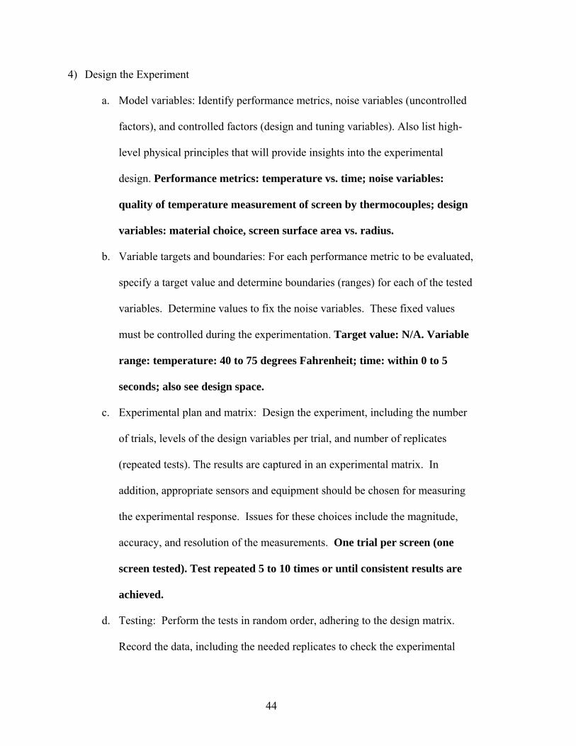
4) Design the Experiment
a. Model variables: Identify performance metrics, noise variables (uncontrolled
factors), and controlled factors (design and tuning variables). Also list high-
level physical principles that will provide insights into the experimental
design. Performance metrics: temperature vs. time; noise variables:
quality of temperature measurement of screen by thermocouples; design
variables: material choice, screen surface area vs. radius.
b. Variable targets and boundaries: For each performance metric to be evaluated,
specify a target value and determine boundaries (ranges) for each of the tested
variables. Determine values to fix the noise variables. These fixed values
must be controlled during the experimentation. Target value: N/A. Variable
range: temperature: 40 to 75 degrees Fahrenheit; time: within 0 to 5
seconds; also see design space.
c. Experimental plan and matrix: Design the experiment, including the number
of trials, levels of the design variables per trial, and number of replicates
(repeated tests). The results are captured in an experimental matrix. In
addition, appropriate sensors and equipment should be chosen for measuring
the experimental response. Issues for these choices include the magnitude,
accuracy, and resolution of the measurements. One trial per screen (one
screen tested). Test repeated 5 to 10 times or until consistent results are
achieved.
d. Testing: Perform the tests in random order, adhering to the design matrix.
Record the data, including the needed replicates to check the experimental
44
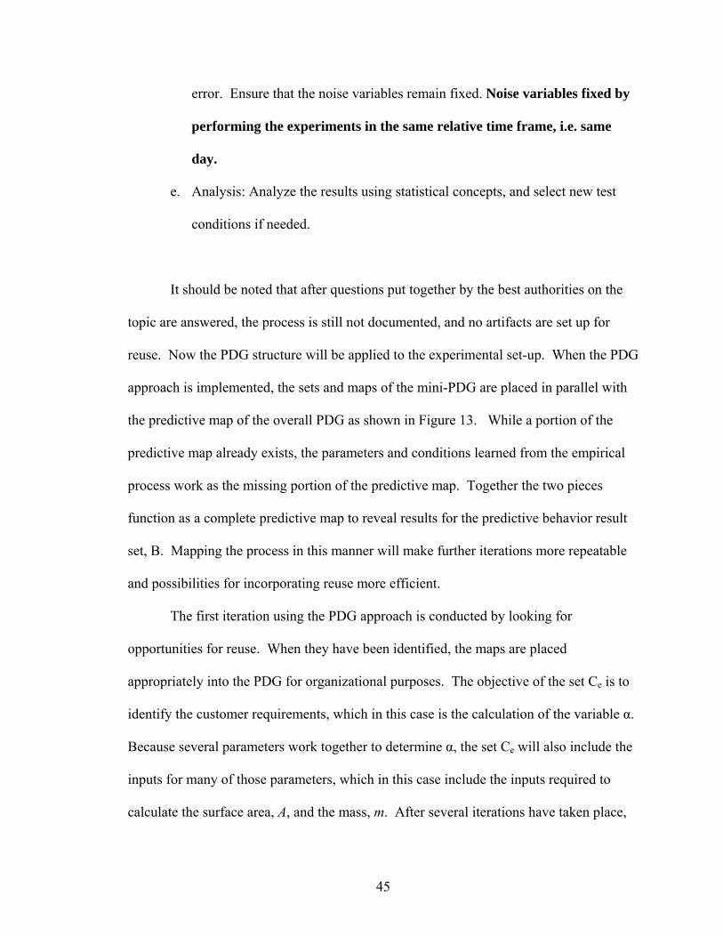
error. Ensure that the noise variables remain fixed. Noise variables fixed by
performing the experiments in the same relative time frame, i.e. same
day.
e. Analysis: Analyze the results using statistical concepts, and select new test
conditions if needed.
It should be noted that after questions put together by the best authorities on the
topic are answered, the process is still not documented, and no artifacts are set up for
reuse. Now the PDG structure will be applied to the experimental set-up. When the PDG
approach is implemented, the sets and maps of the mini-PDG are placed in parallel with
the predictive map of the overall PDG as shown in Figure 13. While a portion of the
predictive map already exists, the parameters and conditions learned from the empirical
process work as the missing portion of the predictive map. Together the two pieces
function as a complete predictive map to reveal results for the predictive behavior result
set, B. Mapping the process in this manner will make further iterations more repeatable
and possibilities for incorporating reuse more efficient.
The first iteration using the PDG approach is conducted by looking for
opportunities for reuse. When they have been identified, the maps are placed
appropriately into the PDG for organizational purposes. The objective of the set Ce is to
identify the customer requirements, which in this case is the calculation of the variable α.
Because several parameters work together to determine α, the set Ce will also include the
inputs for many of those parameters, which in this case include the inputs required to
calculate the surface area, A, and the mass, m. After several iterations have taken place,
45

Figure 13. Empirical Process Used to Complete or Update Predictive Model
an expected range for each parameter input may be appropriate to add to the set Ce. The
acquisition software parameters are stored in the set Ke. All of these parameters are
stored in the set Me. The final 10 steps of the empirical process used in this case are
placed in the map Ie. Results for the variable α are stored in the set Te, and because α is
the only desired result, it is also stored in the set Ue.
1st Iteration, Traditional Approach
Because it is assumed that the original screen material and shape chosen will be
satisfactory for the purpose of the aspirator’s design, a one-time test approach is taken.
Because α is made up of known and unknown variables, it can be split into two parts.
The surface area, A, and the mass, m, are known, while h and cv are unknown. Therefore
the ratio h/cv becomes the unknown variable of interest.
46
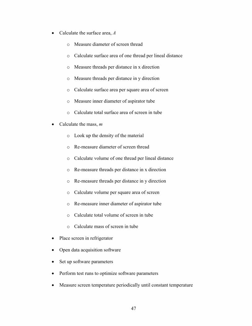
• Calculate the surface area, A
o Measure diameter of screen thread
o Calculate surface area of one thread per lineal distance
o Measure threads per distance in x direction
o Measure threads per distance in y direction
o Calculate surface area per square area of screen
o Measure inner diameter of aspirator tube
o Calculate total surface area of screen in tube
• Calculate the mass, m
o Look up the density of the material
o Re-measure diameter of screen thread
o Calculate volume of one thread per lineal distance
o Re-measure threads per distance in x direction
o Re-measure threads per distance in y direction
o Calculate volume per square area of screen
o Re-measure inner diameter of aspirator tube
o Calculate total volume of screen in tube
o Calculate mass of screen in tube
• Place screen in refrigerator
• Open data acquisition software
• Set up software parameters
• Perform test runs to optimize software parameters
• Measure screen temperature periodically until constant temperature
47

• Start data acquisition
• Clip thermocouples to screen while screen is in refrigerator
• Remove screen and thermocouples from refrigerator into warm room environment
• Stop data acquisition
• Process data into readable format
• Calculate the h/cv ratio
While it may seem unrealistic to repeat several steps in the same test, a sophisticated
empirical process may involve several groups of people conducting different sub
processes. If the process is not planned sufficiently in advance or planned for reuse, the
situation above is realistic. Or one person or group conducting steps on different days
and arriving at a numerical result satisfactory for one portion of the test may not retain
the values of parameters required to arrive at the previously desired result.
2nd Iteration, Traditional Approach
Two methods will be considered for the 2nd iteration. The first method assumes the test
engineer learned from the first iteration and documented that the items re-measured in the
first iteration should be documented, or that there was adequate planning involved for the
second iteration. The second method assumes that a different group of people perform
the iteration, or that the time span is long enough that the original test engineers didn’t
remember the need to document the measured parameters.
• Calculate the surface area, A
o Measure diameter of screen thread (step 1)
48

o Calculate surface area of one thread per lineal distance (step 2)
o Measure threads per distance in x direction (step 3)
o Measure threads per distance in y direction (step 4)
o Calculate surface area per square area of screen (step 5)
o Measure inner diameter of aspirator tube (step 6)
o Calculate total surface area of screen in tube (step 7)
• Calculate the mass, m
o Look up the density of the material (step 8)
o Re-measure diameter of screen thread (step 9)
o Calculate volume of one thread per lineal distance (step 9 or 10)
o Re-measure threads per distance in x direction (step 11)
o Re-measure threads per distance in y direction (step 12)
o Calculate volume per square area of screen (step 10 or 13)
o Re-measure inner diameter of aspirator tube (step 14)
o Calculate total volume of screen in tube (step 11 or 15)
o Calculate mass of screen in tube (step 12 or 16)
• Search for documentation on previous method of conducting test to maintain
consistency
(step 13 or 17)
• Place screen in refrigerator (step 14 or 18)
• Open data acquisition software (step 15 or 19)
• Set up software parameters (step 16 or 20)
• Perform test runs to optimize software parameters (step 17 or 21)
49

• Measure screen temperature periodically until constant temperature
• (step 18 or 22)
• Start data acquisition (step 19 or 23)
• Clip thermocouples to screen while screen is in refrigerator (step 20 or 24)
• Remove screen and thermocouples from refrigerator into warm room environment
(step 21 or 25)
• Stop data acquisition (step 22 or 26)
• Process data into readable format (step 23 or 27)
• Calculate the h/cv ratio (step 24 or 28)
There are 24 steps performed using the first method of the traditional approach, and 28
steps performed using the second method of the traditional approach.
1st Iteration, PDG Approach
The PDG approach includes a strategy of planning in advance and looking for
opportunities for reuse as much as possible. It assumes that process steps are planned in
advance, meaning re-measuring would not take place during the same iteration. It also
assumes that there is a possibility that the test will be performed in the future, therefore
enough documentation is made so that reuse of calculations can be utilized and
parametric operations can be performed. It also assumes that a process map is recorded.
The PDG approach will not split α into two parts. While h and cv are the
unknown variables to be found, the surface area, A, and the mass, m, are retained as
variables.
50

• Calculate the surface area, A
o Measure diameter of screen thread
o Calculate surface area of one thread per lineal distance
o Build in reusable model format
o Measure threads per distance in x direction
o Measure threads per distance in y direction
o Calculate surface area per square area of screen
o Build in reusable model format
o Measure inner diameter of aspirator tube
o Calculate total surface area of screen in tube
o Build in reusable model format
• Calculate the mass, m
o Look up the density of the material
o Calculate volume of one thread per lineal distance
o Build in reusable model format
o Calculate volume per square area of screen
o Build in reusable model format
o Calculate total volume of screen in tube
o Build in reusable model format
o Calculate mass of screen in tube
o Build in reusable model format
• Place screen in refrigerator
• Open data acquisition software
51

• Set up acquisition software parameters
• Document acquisition software parameters
• Perform test runs to optimize acquisition software parameters
• Measure screen temperature periodically until constant temperature
• Start data acquisition
• Clip thermocouples to screen while screen is in refrigerator
• Remove screen and thermocouples from refrigerator into warm room environment
• Stop data acquisition
• Process data into readable format
• Calculate the entire variable α
It is discovered during the first iteration that the surface area, A, and the mass, m,
can depend on several geometric variables such as tube inner diameter, screen material
density, screen thread diameter, and threads per distance in the x and y directions.
Therefore, because this opportunity for reuse is identified, those variables are
incorporated into the calculation documentation, which in this particular experiment is a
simple spreadsheet. A certain group of cells contains all the input variables and others
display final output values. The surface area, A, and the mass, m, become calculation
results of other inputs mentioned above.
2nd Iteration, PDG Approach
• Calculate the surface area, A
o Measure diameter of screen thread
52

o Measure threads per distance in x direction
o Measure threads per distance in y direction
o Measure inner diameter of aspirator tube
• Calculate the mass, m
o Look up the density of the material
o Calculate surface area of one thread per lineal distance, surface area
per square area of screen, total surface area of screen in tube, volume
of one thread per lineal distance, volume per square area of screen,
total volume of screen in tube, and mass of screen in tube all with one
button click (one step)
• Place screen in refrigerator
• Open data acquisition software
• Set up acquisition software parameters according to previous experiment
• Measure screen temperature periodically until constant temperature
• Start data acquisition
• Clip thermocouples to screen while screen is in refrigerator
• Remove screen and thermocouples from refrigerator into warm room environment
• Stop data acquisition
• Process data into readable format
• Calculate the entire variable α
Although this case involves a simple empirical process, the benefits of the PDG
approach are readily observable by comparing the 2nd iterations of the traditional and
53

PDG approaches. By building reusable models, 7 of the 24 or 28 steps are removed from
the process and replaced by a single button click. An additional step is removed due to
process mapping. There are 16 steps performed using the PDG approach compared to 24
or 28 steps using the traditional approach. This represents a 33% to 43% savings in
number of steps alone. Although it is recognized that the actual time saved may or may
not equal 33% to 43%, a reduction in the number of steps will of course have some
correlation with time savings. This savings does not include another significant amount
of time saved as a result of process mapping. Process mapping eliminated the need to
rethink the process or rethink the calculations needed. Even more time is saved because
no effort is required to search for past documents which may be kept in several locations
in the desire to duplicate the methods of the original experiment in order to achieve
consistent results.
Case 2 – Aspirator – A predictive model must be validated
Once the aspirator’s predictive model and its coefficients are established (case 1), the
model must be validated. When the model has proved to sufficiently predict product
performance, the use of the empirical process is complete and design iterations may run
the entire cycle using mathematical models. When a new member of the product family
is introduced which uses a significantly different design, the benefit of reuse of the
validating empirical process is demonstrated. This test case correlates with the second of
the three situations originally mentioned previously.
The aspirator’s performance is modeled with sine wave functions. One sine wave
represents the user’s breathing temperature. The amplitude and frequency of the user’s
54

breathing are measured previously. This sine wave is called the driving function. At the
beginning and end of a breath, the temperature is equal to the environmental temperature.
In the middle of exhalation, the temperature read by the thermocouples is a maximum
due to body heat and fastest velocity of exhaled air. In the middle of inhalation, the
temperature read by the thermocouples is a minimum due to the fastest velocity of
inhaled, colder environmental air. When the aspirator is in use, the air breathed in will be
warmed by the heat conducting material, as in Figure 14.
Figure 14. Breathing Cycle Without Aspirator
55

The objective of the aspirator is to capture heat from exhalation and transfer the
maximum amount of heat to the inhaled air. In Figure 15, the normal breathing cycle is
accompanied by a typical temperature cycle experienced by the screen(s), which is also
modeled by a sine wave. Ideally, the screen would capture all the heat of the exhaled air,
and transfer all that heat to the inhaled air. While the amplitude of the screen’s
temperature cycle in the ideal case would equal the amplitude of the breathing cycle,
realistically the amplitude is less. Ideal heat transfer from the screen to the inhaled air
requires that the temperature cycle of the screen be out of phase with the breathing cycle
such that the . It must retain the heat for an optimal time period. If the screen releases
the heat too quickly or too late, maximum heat will not be transferred to the inhaled air.
The ideal temperature cycle in Figure 15 shows the maximum temperature of the screen
at the finish of exhalation and the minimum heat at the finish of inhalation.
The mathematical model predicting the temperature of the screen is:
)cos()sin()( 2221 tAtAectT t ωω
ωα
ωωα
αα
−−+
−−−= − (4.19)
where T(t) represents the temperature of the screen as a function of time, c1 is a constant
solved for after completing the results of case 1, α is the same as in case 1, A represents
the amplitude of the driving function, and ω is the frequency of the driving function or
the breathing rate of the end user. The only unknown variable is α which was found in
case 1. Theoretically, this model will predict the temperature of the screen(s). An
empirical process is required to validate this model.
56

Figure 15. Typical Aspirator Screen Performance
This validating test assumes that the amplitude, A, and frequency, ω, of a driving
function are first observed through a previous testing procedure in order to optimize other
parameters in the model. The previous test involves placing thermocouples near the
opening of a user’s mouth which is open to approximately the same diameter as the
aspirator tube. The parameters are given values, and a user duplicates the same breathing
pattern breathing through the aspirator. As in case 1, thermocouples are attached to a
small portion of the screen which is not in the breathed airflow in order to prevent the
thermocouples from becoming part of the experimental material, but only a measuring
device. Temperature data points are read at corresponding times and plotted. The
empirical data plot is compared to a theoretical data plot generated from the mathematical
57

model. Specifically, sine wave amplitudes and frequencies are compared. Also, although
the driving function was found previously, it will be monitored again in the validating
test by separate thermocouples in order to compare accuracy against the originally
observed driving function, and to obtain the most accurate values for the driving function
of the validating test.
First, the traditional approach is analyzed. Below are Otto and Wood’s1 steps
with answers supplied in bold while designing the experiment.
1) Plan the prototype
a. Identify the purpose of the prototype in the context of customer needs;
validate amplitude and frequency values of the model predicting screen
temperature
b. Document functionality for these customer needs and identify module
interfaces; Functionality: a static tube with an area of screen inside is used
as a breathing apparatus to observe temperature vs. time; module
interfaces: the edge of the screen is clipped to several thermocouples; the
thermocouples must monitor the material temperature only;
thermocouples are also placed directly in the opening of the mouth in
order to observe driving function properties and accuracy.
c. Determine what physical principles are needed to understand possible
experiments to be performed on a physical model; heat transfer and
conservation of mass principles
58

d. Determine how the physical model would be “measured.” Thermocouples
clipped to the screen will be read constantly by a data acquisition
program (screen is treated as lumped mass, and it is assumed that
thermocouples are in equilibrium with screen; Do the measurement metrics
directly relate to the customer needs and correspond to the engineering
specifications? No, they are raw data that must be processed.
e. Decide if the prototype will be focused or comprehensive, scaled or actual
geometry, and produced from actual materials or not; Focused section of
final product; not scaled, actual material used
f. Determine if rapid prototyping could be used for the physical prototype, and if
so, which technology is appropriate? If not, determine what other fabrication
methods could be used. While rapid prototyping could be used for the
tube, actual material must be used in the screen area for purpose of
experiment
g. Sketch alternative prototype concepts; determine cost, appropriate scale, and
alternative build plans; choose a preferred concept; and develop a fabrication
process plan. Alternative concepts: rapid prototype material or plastic
could be used for tube material. Material cost: rapid prototype material
or plastic, inexpensive screen; time: 4-6 hours. Appropriate scale: actual
scale maintained. Alternative build plans: none considered. Fabrication
process plan: a rapid prototype of the aspirator tube could be built in two
sections with small holes placed near the mouth end, or a plastic tube
which fits loosely into another plastic tube could be used. Both tubes are
59

cut to appropriate length and small holes are placed near the mouth end.
The appropriate number of screens is cut into circular shape. A small
portion of the screen(s) is wrapped around each thermocouple tip. The
plastic tubes are fit together, sandwiching the screen(s) and thermocouple
tips. The small hole is placed in the tube near the mouth end so
thermocouples can measure driving function properties.
h. Determine how the prototype will be tested, aspirator is placed in user’s
mouth while user attempts to breathe at prescribed amplitude and
frequency, what factors will be controlled to minimize experimental error,
thermocouple tips touch maximum area of screen and are kept out of cool
environment; what responses will be measured and with what sensors,
temperature of screen measured over time with thermocouples, how many
tests will be conducted/replicated, only one iteration needed, but conducted
over a time period until consistent results are achieved, will the tests be
destructive or nondestructive, nondestructive, and what the desired accuracy
of the measurements is; accurate enough so that final predictive equation is
accurate within 5% margin.
2) Plan the design space
a. Assume a design space. This assumption implies a restriction on the possible
design choices selected by the product development team, implying a
simplification or model. N/A for validation.
b. Assume a performance metric. How does our metric really measure activities
experienced by a consumer of our product? In a dynamic environment? The
60

metric is temperature in degrees Fahrenheit. The consumer will
experience an increased air temperature during inhalation, therefore
temperature is a worthwhile metric.
c. What effects will variations in the surface, material wear, environment, or any
other uncontrollable factor have on our objective? The factor of greatest
inaccuracy in the experiment is the percent of surface area on the
thermocouple tips covered by the screen.
3) Validate the design space to make sure it’s complete, yet judicious so resources are
not wasted. Not applicable to the purposes of this thesis.
a. Are we sure that the proper variables have been chosen? Do we need to
contemplate high-level physical principles to obtain additional insights? Does
there exist a more effective choice of variables for experimentation?
b. Are we sure that the range of the variables and their number is not too broad,
unnecessarily complicating the experiments?
c. What is the trade-off point, for the development team, between the cost of
varying more variables versus expected payoff in performance increase?
4) Design the Experiment
a. Model variables: Identify performance metrics, noise variables (uncontrolled
factors), and controlled factors (design and tuning variables). Also list high-
level physical principles that will provide insights into the experimental
design. Performance metrics: temperature vs. time; noise variables:
quality of temperature measurement of screen by thermocouples; design
variables: N/A for validation.
61
b. Variable targets and boundaries: For each performance metric to be evaluated,
specify a target value and determine boundaries (ranges) for each of the tested
variables. Determine values to fix the noise variables. These fixed values
must be controlled during the experimentation. Target value: within 5% of
predicted values. Variable range: temperature: 80 to 90 degrees
Fahrenheit; time: within 0 to 50 seconds; also see design space.
c. Experimental plan and matrix: Design the experiment, including the number
of trials, levels of the design variables per trial, and number of replicates
(repeated tests). The results are captured in an experimental matrix. In
addition, appropriate sensors and equipment should be chosen for measuring
the experimental response. Issues for these choices include the magnitude,
accuracy, and resolution of the measurements. One trial is expected for
validation. Although one sine wave period is needed for final results, at
least 100 breath periods will be monitored and averaged.
d. Testing: Perform the tests in random order, adhering to the design matrix.
Record the data, including the needed replicates to check the experimental
error. Ensure that the noise variables remain fixed. Noise variables fixed by
performing the experiments in the same relative time frame, i.e. same
day.
e. Analysis: Analyze the results using statistical concepts, and select new test
conditions if needed.
62

It should again be noted that after questions put together by the best authorities on
the topic are answered, the process is still not documented, and no artifacts are set up for
reuse. Now the PDG structure will be applied to the experimental set-up. When the PDG
approach is implemented, the sets and maps of the mini-PDG replace the testing
procedure map, I, of the overall PDG as shown in Figure 16. Mapping the process in
this manner will make further iterations more repeatable and possibilities for
incorporating reuse more efficient.
Figure 16. Process Used to Validate Predictive Model
The first iteration using the PDG approach is conducted by looking for
opportunities for reuse. When they have been identified, the maps are placed
appropriately into the PDG for organizational purposes. The objective of the set Ce is to
identify the customer requirements, which in this case includes inputs such as the age of
63

end user, the expected work out capacity, and the percent accuracy defining the
difference between the predictive and empirical models. The map De converts the age
input into a mouth size, aspirator tube outer diameter and screen cut diameter; and it
converts the work out capacity into the expected driving function’s amplitude and
frequency. The set Ke includes somewhat constant variables such as tube material
thickness, lengths and taper angle. The acquisition software parameters are also stored in
the set Ke. All of these parameters are stored in the master parameter list Me. The final
12 steps of the empirical process used in this case are placed in the map Ie. Results for
the percent accuracy are stored in the set Te, and because the percent accuracy is the only
desired result, it is also stored in the set Ue.
1st Iteration, Traditional Approach
The traditional approach assumes that the validation test is a one time test because it is
simply validation and not a performance of several experimental trials. The tube is then
cut to fit the single screen set-up which is thought to perform best in the aspirator. Figure
17 shows the tube sections with a cut out cross section. The screen is bent as the sections
are pushed together. The screen (and thermocouples) fit perfectly in the space between
the tube sections. Following are the steps required to complete the empirical process.
• Build aspirator tube
o Build CAD models of aspirator tube sections
o Cut tube lengths and turn on lathe to alter diameter for fitting
o Cut screen sections
64

Figure 17. Aspirator Tube Showing Cross-Section, Traditional Approach
o Place thermocouples in screen
o Assemble aspirator tube sections, screen, and thermocouples
• Open data acquisition software
• Set up software parameters
• Perform test runs to optimize software parameters
• Start metronome (user listens to metronome to most closely mimic previously
recorded data)
• Place aspirator in user’s mouth and breath at prescribed rate
• Start & stop data acquisition
• Process data into readable format (plot points, calculate average frequencies &
amplitudes)
• Compare results to predictive model
2nd Iteration, Traditional Approach
An unexpected second iteration is required because it is found that a different size screen
or greater number of screens is needed to fulfill the requirements for the aspirator. A new
65

set of tubes must be constructed because the original tube sections will not accommodate
the larger space and bending limits of the new screen apparatus.
• Build aspirator tube
o Build new CAD models of aspirator tube sections
o Cut tube lengths and turn on lathe to alter diameter for fitting
o Cut screen sections
o Place thermocouples in screen
o Assemble aspirator tube sections, screen, and thermocouples
• Search for documentation on previous method of conducting test to maintain
consistency
• Open data acquisition software
• Set up software parameters
• Perform test runs to optimize software parameters
• Start metronome (user listens to metronome to most closely mimic previously
recorded data)
• Place aspirator in mouth and breath at prescribed rate
• Start & stop data acquisition
• Process data into readable format (plot points, calculate average frequencies &
amplitudes)
• Compare results to predictive model
66

1st Iteration, PDG Approach
The PDG approach includes a strategy of planning in advance and looking for
opportunities for reuse as much as possible. It also assumes that there is a possibility that
the test will be performed in the future; therefore, parametric models are constructed
instead of static models, testing apparatus is planned in advance to be used with a range
of parameters, and enough documentation is made so that reuse of calculations can be
utilized and parametric operations can be performed. It also assumes that a process map
is recorded.
A different tube design is used as a result of DFR (designing for reuse). It is
assumed that a range of screen thicknesses may possibly be validated in the future.
Therefore, angled mating sections are designed into the tube interfacing portions as show
in Figure 18. As the tube sections are pushed together, a range of screen thicknesses will
function in the available space, and they will not need to bend as much as the design used
in the traditional approach.
• Build aspirator tube
o Build parametric CAD models of aspirator tube sections
o Cut tube lengths and turn on lathe to alter diameter for fitting
o Cut screen sections
o Place thermocouples in screen
o Assemble aspirator tube sections, screen, and thermocouples
• Open data acquisition software
• Set up software parameters
• Perform test runs to optimize software parameters
67
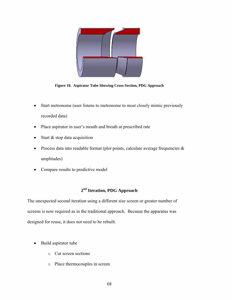
Figure 18. Aspirator Tube Showing Cross-Section, PDG Approach
• Start metronome (user listens to metronome to most closely mimic previously
recorded data)
• Place aspirator in user’s mouth and breath at prescribed rate
• Start & stop data acquisition
• Process data into readable format (plot points, calculate average frequencies &
amplitudes)
• Compare results to predictive model
2nd Iteration, PDG Approach
The unexpected second iteration using a different size screen or greater number of
screens is now required as in the traditional approach. Because the apparatus was
designed for reuse, it does not need to be rebuilt.
• Build aspirator tube
o Cut screen sections
o Place thermocouples in screen
68

o Assemble aspirator tube sections, screen, and thermocouples
• Open data acquisition software
• Set up acquisition software parameters according to previous experiment
• Start metronome (user listens to metronome to most closely mimic previously
recorded data)
• Place aspirator in mouth and breath at prescribed rate
• Start & stop data acquisition
• Process data into readable format (plot points, calculate average frequencies &
amplitudes)
• Compare results to predictive model
Like case 1, and although this case involves a simple empirical process, the
benefits of the PDG approach are readily observed by comparing the 2nd iterations of the
traditional and PDG approaches. By building reusable models and mapping the process
into a readily available format, 4 of the 14 steps are removed from the process when a
different screen set-up is tested by a user of an equivalent age to the original user. The
two longest steps of the empirical process were eliminated because the DFR principle
(designing for reuse) was applied to the design of the apparatus. If in fact the second
iteration were required for a small child instead of an adult and the apparatus were the
wrong size, the CAD model would not need to be rebuilt but simply updated because of
the parametric capability built into it. In this case 3 of the 14 steps are removed from the
empirical process. This represents a 21% to 29% time savings in number of steps alone,
however the time savings would be much greater if the percentage of total time were
69

measured due to the significance of building a CAD model and manufacturing the
apparatus. This time savings does not include another significant amount of time saved
as a result of process mapping. Process mapping eliminated the need to rethink the
process or rethink the calculations needed. Even more time is saved because no effort is
required to search for past documents. These documents may be kept in several locations
in the desire to duplicate the methods of the original experiment in order to achieve
consistent results.
Case 3 – Daisy Mixer – A predictive model does not exist
Because an accurate predictive CFD model is not available, the effect of the shape of the
daisy mixer on vortex strength, or vorticity, and location is designed through empirical
processes. A wind tunnel and data acquisition system were available and a method was
required to test various shapes of the daisy mixer. Two products needed to be designed
and built: 1) a method of providing and controlling two different airspeeds to be passed
around the mixer, and 2) the daisy mixer test-piece itself. It can be seen that the process
of designing and testing the test-piece or prototype resembles a complete product
development process. Figure 19 shows a summary of the prototype development process
compared to the previously mentioned NASA stage gate product development process.
Following is an overview of the experimental set-up before comparisons are made
between current and proposed methods. The daisy mixer used on a turbine engine is
attached to a circular outlet and the two flows are concentric. For convenience of
measurement purposes, the circular mixer is “unwrapped” or linearized so that x,y,z
coordinates may be used, and the two airflows in the experiment are separated by a planar
70

Figure 19. Prototype Design Involves Complete Design Process
wall. The wind tunnel used is a 15” by 15” square tunnel with air being pushed through
it. The air entering the tunnel is evenly distributed and smoothed by a series of screens
upstream of the tunnel. Inside the tunnel a splitter was placed to divide the airflow into
two different speeds. The splitter is made of a 4 foot long thin walled box which fits into
half the tunnel, thus splitting the flow into two halves of approximately equal area.
Inside the splitter box is a series of perforated metal plates which slow the airflow.
Honeycomb material follows the plates to smooth the airflow. Airflows were tested to
ensure even distribution of airspeed. Adjustments were made until a 4:1 airspeed ratio
was achieved between the two halves of the tunnel. Because the end of the splitter box
was flush with the end of the tunnel and because it was not desired to drill test piece
mounting holes into the existing wind tunnel, a ten inch extension of the tunnel was
constructed to hold the test piece. The test piece is mounted vertically and positioned to
be flush with the divider wall in the middle of the tunnel. An additional 2 foot Plexiglas
71

extension was placed on the tunnel to maintain flow conditions and provide a transparent
medium for data acquisition cameras. Figure 20 shows the final portion of the wind
tunnel containing the splitter and test piece and the tunnel extension.
Figure 20. Daisy Mixer General Set-up
Data acquisition is achieved by inserting light scattering particles into the air
intake of the wind tunnel light enough to follow the airflow. Figure 21 and Figure 22
show the PIV cameras and laser sheet created by the PIV system, respectively. Two
horizontal sheets of laser light separated by a short time interval illuminate a plane of
particles and two high resolution CCD cameras capture 3D movement of the particles.
Data processing and post processing calculate airflow vectors in the sheet. Many sheets
of data are taken at successive altitudes until a 3D block of data exists and calculations
can be performed on any desired plane within the block. Additional post processing
calculated vorticity in the airflow. This data acquisition system is called particle image
velocimetry (PIV).
72

Figure 21. PIV Cameras
Figure 22. PIV Laser Sheet As the PDG architecture is targeted to structure the Detailed Design and Prototype
& Test phases, these portions will be the focus of comparison between current and
proposed methods. Below are Otto and Wood’s1 steps with answers supplied in bold
while designing the mixer test piece.
73

1) Plan the prototype
a. Identify the purpose of the prototype in the context of customer needs;
Identify effect of geometry shape on vorticity and position
b. Document functionality for these customer needs and identify module
interfaces; Functionality: a static piece of geometry is placed in the midst
of two airflows and its shape mixes those airflows; module interfaces: the
leading edge of the mixer is flush with the trailing edge of upstream
geometry.
c. Determine what physical principles are needed to understand possible
experiments to be performed on a physical model; Relationship between
airflow vectors and vorticity
d. Determine how the physical model would be “measured.” Particle Image
Velocimetry (PIV) system photographs airflow and displays airflow
vectors. Vectors are then analyzed to determine vorticity and position; Do
the measurement metrics directly relate to the customer needs and correspond
to the engineering specifications? Yes.
e. Decide if the prototype will be focused or comprehensive, scaled or actual
geometry, and produced from actual materials or not; Focused geometry; not
scaled but converted from radial to linear geometry; rapid prototype
materials used.
f. Determine if rapid prototyping could be used for the physical prototype, and if
so, which technology is appropriate? If not, determine what other fabrication
methods could be used. Rapid prototype plaster materials OK.
74

g. Sketch alternative prototype concepts; determine cost, appropriate scale, and
alternative build plans; choose a preferred concept; and develop a fabrication
process plan. Alternative concepts: keep geometry radial. Idea rejected
because of difficulty to accurately measure vortices in a small tunnel.
Material cost: $20 / rapid prototype; time: 2 days. Appropriate scale:
actual scale maintained. Alternative build plans: none considered because
of complex shape. Preferred concept: linear geometry. Fabrication
process plan: build rapid prototype in sections, strengthening epoxy used
as protective layer and as glue to hold sections together.
h. Determine how the prototype will be tested, placed in wind tunnel, what
factors will be controlled to minimize experimental error, airflow speeds kept
constant; measurements taken of vortex where tunnel walls have minimal
influence; what responses will be measured and with what sensors, airflow
vectors measured by PIV system, how many tests will be
conducted/replicated, indefinite, will the tests be destructive or
nondestructive, nondestructive, and what the desired accuracy of the
measurements is. Relative vorticity results comparing effects of geometry
are more important than actual magnitudes. Accuracy controlled
between iterations by keeping setup constant and changing only the test
piece geometry.
2) Plan the design space
a. Assume a design space. This assumption implies a restriction on the possible
design choices selected by the product development team, implying a
75

simplification or model. According to the image above, the lobe radius
ratio will be altered between 2:1 and 1:1.
b. Assume a performance metric. How does our metric really measure activities
experienced by a consumer of our product? In a dynamic environment?
Vorticity is assumed to correlate to sound reduction. Results from the
two tests will be compared relatively.
c. What effects will variations in the surface, material wear, environment, or any
other uncontrollable factor have on our objective? Because surface finish
will be the same on both parts, it is assumed to not be a factor.
Environment, distance of the study focus area, the middle of the mixer, is
calculated to be far enough from the tunnel walls that environment will
not make a significant impact on the results.
3) Validate the design space to make sure it’s complete, yet judicious so resources are
not wasted. Not applicable to the purposes of this thesis.
a. Are we sure that the proper variables have been chosen? Do we need to
contemplate high-level physical principles to obtain additional insights? Does
there exist a more effective choice of variables for experimentation?
b. Are we sure that the range of the variables and their number is not too broad,
unnecessarily complicating the experiments?
c. What is the trade-off point, for the development team, between the cost of
varying more variables versus expected payoff in performance increase?
76

4) Design the Experiment
a. Model variables: Identify performance metrics, noise variables (uncontrolled
factors), and controlled factors (design and tuning variables). Also list high-
level physical principles that will provide insights into the experimental
design. Performance metrics: airflow vectors analyzed for vorticity; noise
variables: ambient air temperature and pressure, humidity; design
variables: large lobe radius, lobe radius ratio.
b. Variable targets and boundaries: For each performance metric to be evaluated,
specify a target value and determine boundaries (ranges) for each of the tested
variables. Determine values to fix the noise variables. These fixed values
must be controlled during the experimentation. Target value: no specific
target value, but relative comparison of results. Variable range: see
design space.
c. Experimental plan and matrix: Design the experiment, including the number
of trials, levels of the design variables per trial, and number of replicates
(repeated tests). The results are captured in an experimental matrix. In
addition, appropriate sensors and equipment should be chosen for measuring
the experimental response. Issues for these choices include the magnitude,
accuracy, and resolution of the measurements. Two trials: one for each
ratio. Tests not repeated because average of flow values is taken over
time.
d. Testing: Perform the tests in random order, adhering to the design matrix.
Record the data, including the needed replicates to check the experimental
77
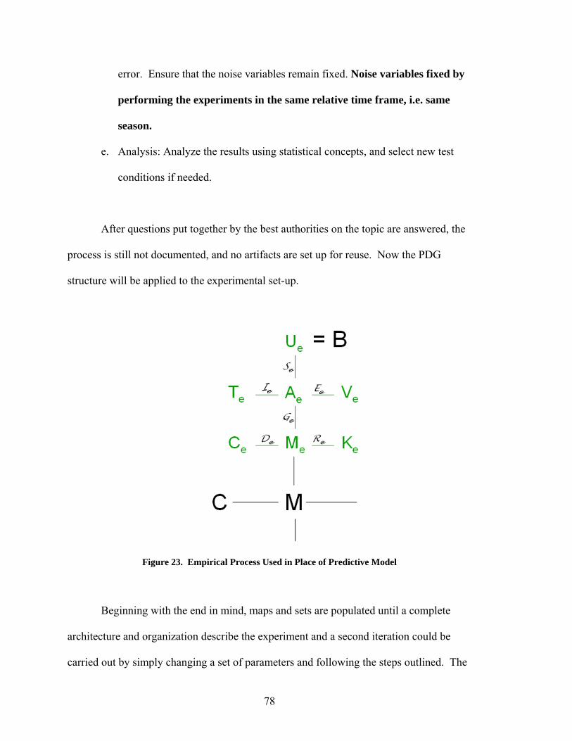
error. Ensure that the noise variables remain fixed. Noise variables fixed by
performing the experiments in the same relative time frame, i.e. same
season.
e. Analysis: Analyze the results using statistical concepts, and select new test
conditions if needed.
After questions put together by the best authorities on the topic are answered, the
process is still not documented, and no artifacts are set up for reuse. Now the PDG
structure will be applied to the experimental set-up.
Figure 23. Empirical Process Used in Place of Predictive Model
Beginning with the end in mind, maps and sets are populated until a complete
architecture and organization describe the experiment and a second iteration could be
carried out by simply changing a set of parameters and following the steps outlined. The
78

main PDG structures the design of the daisy mixer to be mounted to a turbine engine.
The physical behavior is unknown at this stage and the set B is desired. A predictive
model does not exist and therefore the predictive map P must be substituted with an
empirical process, as shown in Figure 23. The sub-PDG structures the empirical process
and is inserted into the main PDG, and the deliverables set Ue becomes equal to the set B.
Ue must contain data relating geometry to vorticity. Te contains the vorticity results of
one iteration. Ie is the testing procedure and maps the artifacts into Te. Ie contains
models and procedures used in the test itself, including PIV data processing and post
processing software models. Ae contains the solid model of the test piece, the test piece
hardware, test instructions, the rapid prototype build model, finishing instructions, a
model showing the test set-up and component placement, and testing procedure
instructions. Ge contains parametric solid model(s) of the test piece, parametric
manufacturing models and documents such as the rapid prototype model and finishing
instructions, parametric models showing the test set-up and component placement, and a
parametric document of testing procedure instructions. Ae and Ge seem similar, however
the difference is that Ae contains instantiations of Ge, and Ge, as a map, contains
parametric models and documents. The master parameter list Me contains all the
parameters needed for every model and document contained in the maps Ge and Ie. Ce
contains the customer requirements vorticity and small lobe radius. De maps the
customer requirements found in Ce to Me and cannot be formulated until trends from the
test results appear. The results from Te will be compared to Ce so that De can be updated.
The parameters found in Ce will determine several parameters found in Me. Re contains
the rules to map remaining parameters found in Ke to Me. Ve will contain a record of all
79
the parameters that went into every model, which is an instantiation of Me. It will also
contain every component of Ae. Ee as the selection procedure in this case simply
specifies that all of Me and all of Ae are to be vaulted. Se takes all the results from Te and
compiles them into a usable format showing patterns of data.
Comparison of Traditional Method Vs. Proposed Method
Because the time required to complete certain tasks can vary greatly, stopwatch time
comparisons will not be used to compare traditional empirical process methods against
the proposed empirical process methods. Instead, a task list summarizing steps to
conduct two test iterations for each method will be compiled. However, general time
estimates will be used to demonstrate an idea of the time savings.
Over one year of time had passed between the first and second iterations using the
traditional method. While conducting the second iteration, the importance of
documentation of process steps as well as documentation of the process itself was very
evident because the process execution was not fresh in memory. This pattern of
significant time between iterations or change of employees conducting consecutive tests
is not uncommon in industry.
Following is documentation of the four iterations. The PDG approach is assumed
to be conducted in parallel with the traditional approach to avoid the argument that time
was saved through a learning curve occurring during the traditional approach. Typical
man hours for each step are documented.
80

Notes on the 2nd iteration of the traditional approach:
Although much documentation was made of various experimental steps and it was
all thought to be placed in logical locations, the absence of process mapping resulted in
incomplete documentation, as well as wasted time due to searching for the
documentation. It was important to duplicate original test methods and parameters as
much as possible to correlate iteration results accurately. Time dedicated to searching for
documentation includes the tedious process of working through original experimental
data to find needed information when documentation was not complete. Therefore,
during some steps of the testing process, more time was required for the second iteration
than the first because of the need to duplicate the methods and parameters of the first
iteration. It takes significantly less time to document steps taken than to figure out what
to do again.
Notes on the 1st iteration of the PDG approach:
Because the process of the second iteration is fresh in mind, and it assumed that
the first iteration of the PDG approach would take the place of the first iteration using the
traditional approach, the man hours required for steps in this first iteration are assumed to
be equal to those required for the first iteration using the traditional approach. Different
and additional steps are noted in bold. As discovered by Teare30, extra steps of writing
documentation and setting up reuse process software require additional 10% investment
of time on top of going through the first iteration. Hence, the bold steps require an extra
10% of the total time.
81

1st Iteration, Traditional Approach:
Preparation – One Time Events
• Construct plexi-glass box to ensure a proper velocity ratio across the lobe (30
hours)
• Insert box into wind tunnel, and fasten box to tunnel (2 hours)
• Build frame around mixer lobe (5 hours)
• Align mixer with splitter plate (1 hour)
• Fasten mixer to the frame (.5 hour)
• Assemble extension to extend the wind tunnel test section beyond the trailing
edge of the lobe (5 hours)
• Write Matlab program to view results (reuse considered but instructions not
documented) (10 hours)
Iteration Process Steps – Modeling the Mixer
• Build axially symmetric CAD model of mixer (10 hours)
• Decide design modifications to linearize axially symmetric CAD model (5 hours)
• Build linear CAD model of mixer (15 hours)
• Add end caps to facilitate assembly (1 hour)
• Divide CAD model into 3 parts to accommodate rapid prototype machine (1 hour)
Manufacture the test piece
• Take tunnel measurements and scale down STL file (.5 hour)
• Print 3 sections using rapid prototyping machine (3 hours)
82
• Epoxy 3 sections (epoxy acts as glue, surface finish, and stiffener transforming 3
sections into the full test piece) (2 hours)
• Sand test piece once it’s dry (1 hour)
Debugging apparatus & test rig
• Test one of two cameras - results: Laser reflections a major issue (2 hours)
• Apply black paint to many surfaces (2 hours)
• Apply wavelength absorbing paint to test piece (3 hours)
• Place black construction paper at key locations (3 hours)
• Calibrate cameras (3 hours)
• Adjust tunnel airspeed until velocity ratio is correct (5 hours)
• Optimize parameters for velocity ratio by running several test runs (5 hours)
Conducting test
• Prepare software for test (1 hour)
• Take data (some procedures documented) (3 hours)
o Start tunnel at appropriate speed
o Turn on mist
o Loop:
Turn on lasers
Start data acquisition
Turn off lasers
Move location of laser sheet plane
83

• Process data (some procedures documented) (3 hours)
o Set parameters
• Post process data (some procedures documented) (1 hour)
o Set parameters
• Reorganize data in preparation for results calculation
• Calculate & interpret results
2nd Iteration, Traditional Approach:
Manufacture new test piece
• Build new geometric model with different dimensions (15 hours)
• Divide CAD model into 3 parts to accommodate rapid prototype machine (1 hour)
• Search for rapid prototype scaling factor documentation (.25 hours)
• Print 3 sections using rapid prototyping machine (3 hours)
• Epoxy 3 sections (2 hours)
• Sand test piece once it’s dry and paint test piece with laser wavelength absorbing
paint (1 hour)
Set up test rig
• Place splitter in tunnel (.25 hours)
• Place test piece frame on end of tunnel (.25 hours)
• Insert test piece into frame (.25 hours)
• Place tunnel extension on end of tunnel (.25 hours)
84

Debugging apparatus & test rig
• Search for photos showing locations of black construction paper (.25 hours)
• Place black construction paper at key locations (1 hour)
• Search for documentation on calibrating cameras (.5 hours)
• Calibrate cameras (3 hours)
• Search for documentation on adjusting velocity ratio (.25 hours)
• Adjust tunnel airspeed until velocity ratio is correct (.25)
• Search for documentation (if it exists) on optimized parameters (.25 hours)
• Optimize parameters for velocity ratio by running several test runs (5 hours)
Conducting test
• Prepare software for test (1 hour)
• Take data
o Search for documentation on tunnel speed (.25 hours)
o Start tunnel at appropriate speed (0 hours)
o Turn on mist
o Loop:
Turn on lasers
Start data acquisition
Turn off lasers
Search for documentation on laser sheet height change (.25
hours)
Move location of laser sheet plane (how much?)
85

• Process data (3 hours)
o Search for documentation on data processing parameters and their
reasoning (.25 hours)
o Set parameters (how to know reasoning behind parameters set?)
• Post process data (1 hour)
o Search for documentation on data post processing parameters and
their reasoning (.25 hours)
o Set parameters (how to know reasoning behind parameters set?)
• Search for documentation on data reorganization (.5 hours)
• Reorganize data in preparation for results calculation
• Calculate & interpret results
1st Iteration, PDG approach
Set up process mapping (extra 10% of total time of first iteration of traditional
approach)
• Set up PDG organization
• Map complete process on paper and in user software
• Write up complete documentation while performing 1st iteration
• Place documentation into appropriate folders, organized into sets and maps
under a PDG folder
86

Preparation – One Time Events
• Construct plexi-glass box to ensure a proper velocity ratio across the lobe (30
hours)
• Insert box into wind tunnel, and fasten box to tunnel (2 hours)
• Build frame around mixer lobe (5 hours)
• Align mixer with splitter plate (1 hour)
• Fasten mixer to the frame (.5 hour)
• Assemble extension to extend the wind tunnel test section beyond the trailing
edge of the lobe (5 hours)
• Write Matlab program to view results (written to be reused, document all
instructions) (10 hours)
Iteration Process Steps – Modeling the Mixer
• Build axially symmetric CAD model of mixer (10 hours)
• Decide design modifications to linearize axially symmetric CAD model (5 hours)
• Plan and build CAD parametric model (designed for reuse) (15 hours)
• Build end caps into parametric CAD model to facilitate assembly (1 hour)
• Build sectioning into parametric CAD model to accommodate rapid
prototype machine (.5 hour)
Manufacture the test piece
• Take tunnel measurements and scale down STL file (.5 hour)
• Print 3 sections using rapid prototyping machine (3 hours)
• Epoxy 3 sections (epoxy acts as glue, surface finish, and stiffener transforming 3
sections into the full test piece) (2 hours)
87
• Sand test piece once it’s dry (1 hour)
Debugging apparatus & test rig
• Test one of two cameras - results: Laser reflections a major issue (2 hours)
(document issues and solutions)
• Apply black paint to many surfaces (2 hours) (document placement of painted
areas)
• Apply wavelength absorbing paint to test piece (3 hours) (document all issues
and locations)
• Place black construction paper at key locations (3 hours) (document exact
positions of key locations)
• Calibrate cameras (3 hours) (document all steps taken and methods used)
• Adjust tunnel airspeed until velocity ratio is correct (5 hours) (document all
information about trial runs)
• Optimize parameters for velocity ratio (5 hours) (document all parameters and
reasoning)
• Strategically place all documentation into process map
Conducting test
• Prepare software for test (1 hour) (document every parameter and reasoning)
• Take data (3 hours)
o Start tunnel at appropriate speed
o Turn on mist
o Loop:
Turn on lasers
88

Start data acquisition
Turn off lasers
Move location of laser sheet plane (document every parameter
and reasoning)
• Process data (3 hours)
o Set parameters (document every parameter and reasoning)
• Post process data (1 hour)
o Set parameters (document every parameter and reasoning)
• Reorganize data in preparation for results calculation (document all steps and
reasoning)
• Calculate & interpret results
• Strategically place all documentation into process map
2nd Iteration, PDG approach
The test engineer follows the process map and documentation throughout entire
experiment. Process software leads through the steps and provides data, and can even
provide necessary parameters in necessary format as input to software models. All
information needed is provided just in time for the next step. The documentation is
assumed to be adequately clear that following the map and documentation requires no
learning curve.
Manufacture new test piece
• Reuse: parametric CAD model (alter parameters) (.25 hours)
• Print 3 sections using Zcorp rapid prototyping machine (3 hours)
89

• Epoxy 3 sections (2 hours)
• Sand test piece once it’s dry and paint test piece with laser wavelength absorbing paint (1 hour)
• [saved 16 hours]
Set up test rig
• Place splitter in tunnel (.25 hours)
• Place test piece frame on end of tunnel (.25 hours)
• Insert test piece into frame (.25 hours)
• Place tunnel extension on end of tunnel (.25 hours)
Debugging apparatus & test rig
• Reuse process map: Place black construction paper at key locations (.25 hours)
• Reuse process map: Calibrate cameras (2 hours)
• Reuse process map: Adjust tunnel airspeed until velocity ratio is correct (.25 hours)
• Reuse process map: Optimize parameters for velocity ratio by running several test runs (1 hour)
• [saved 7 hours]
Conducting test
• Reuse process map: Prepare software for test (.5 hours)
• Take data
o Start tunnel at appropriate speed (0 hours)
o Turn on mist
o Loop:
Turn on lasers
Start data acquisition
Turn off lasers
Reuse process map: Move location of laser sheet plane
90
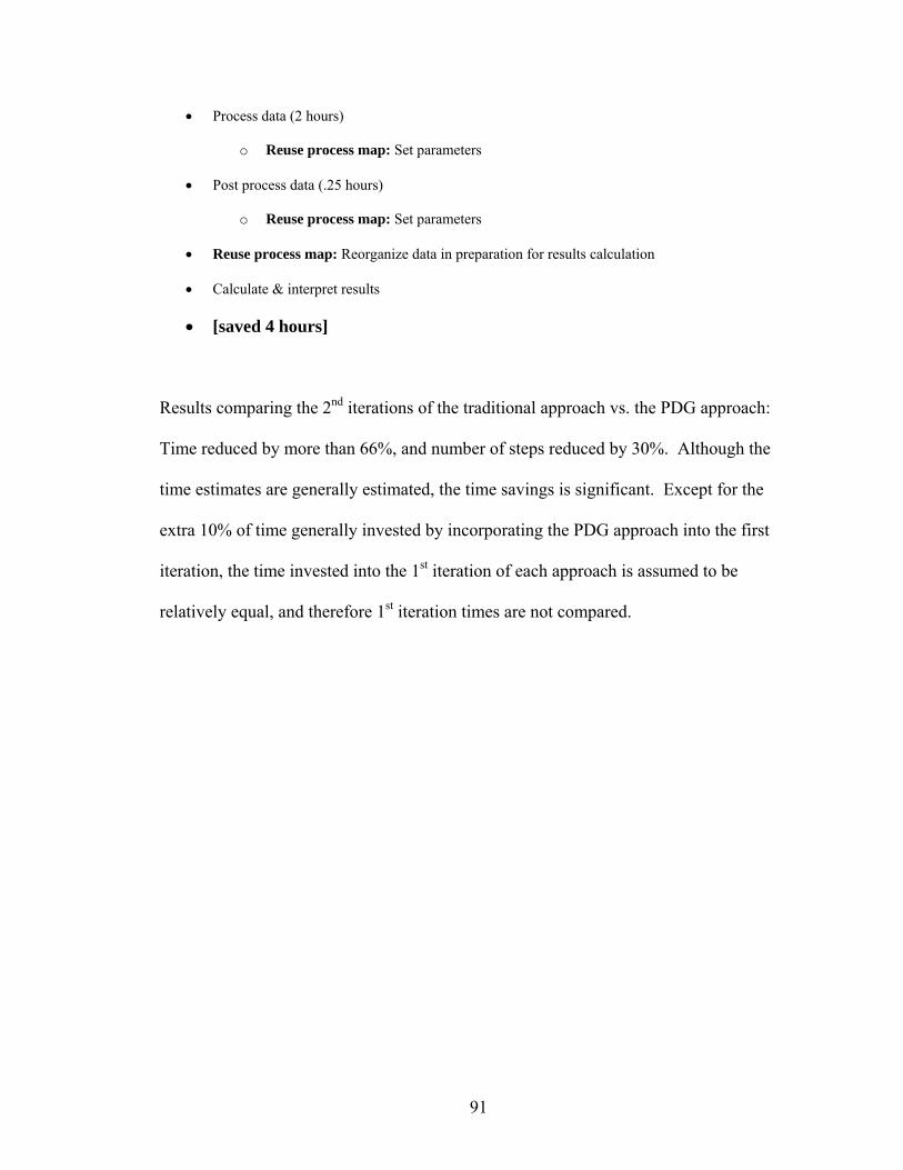
• Process data (2 hours)
o Reuse process map: Set parameters
• Post process data (.25 hours)
o Reuse process map: Set parameters
• Reuse process map: Reorganize data in preparation for results calculation
• Calculate & interpret results
• [saved 4 hours]
Results comparing the 2nd iterations of the traditional approach vs. the PDG approach:
Time reduced by more than 66%, and number of steps reduced by 30%. Although the
time estimates are generally estimated, the time savings is significant. Except for the
extra 10% of time generally invested by incorporating the PDG approach into the first
iteration, the time invested into the 1st iteration of each approach is assumed to be
relatively equal, and therefore 1st iteration times are not compared.
91

92
Chapter 5. Implementation of PDG Approach
To assist the reader in understanding how to implement the PDG approach, the steps
taken to conduct the daisy mixer test case will be detailed as an example to follow.
Recalling from chapter 3, there are three fundamental steps to the implementation of the
PDG approach:
1) Decomposition of a product’s design process
2) Organization and development of relationships
3) Identify and implement process and task reuse
Before beginning the decomposition process, it is noted that the initial constraints
of the experiment include using an available wind tunnel with a 15 inch by 15 inch square
opening and a PIV laser data acquisition system. First, to decompose the design process
using a “backwards mapping” technique, the steps required to arrive at the final result are
examined. The final results desired are the location and strength of the vortices formed
by high speed air flowing over one side of the test piece, and low speed air flowing over
the other side. In order to calculate these numbers, the circulation of the air must be
known in a succession of planes perpendicular to the airflow. In order to find the
circulation of the air, data must be taken showing airflow patterns and vectors in the
regions of interest. Because the prescribed PIV system cannot take data in the planes of
interest, data is taken in several planes parallel to the airflow and transposed using data
processing software. In order to take the airflow data, the PIV system must be set up to
photograph the correct regions of airspace, a test piece must be placed in the airflow to
93

produce the data, and the available wind tunnel must be used to produce regulated
airflow. This first portion of the backwards mapping is shown in Figure 24. It is a first
draft of the backwards map which will later include details to fill in gaps of missing
information or task steps.
Figure 24. Daisy Mixer Backwards Map 1
Next, the backwards mapping is continued from each of the three tasks, as shown
in Figure 25. In order to set up the PIV system to take data in the appropriate regions, the
appropriate regions must be determined, and space must be available to set up the needed
PIV apparatus. In order to place a test piece in an airflow, a test piece must be
constructed. To construct a test piece, a CAD model must be built. To build a CAD
model, the dimensions of the test piece must first be determined. In order to have the
available wind tunnel produce regulated airflow, the appropriate airspeeds must be
determined and a form of producing secondary airflow must be provided.
94
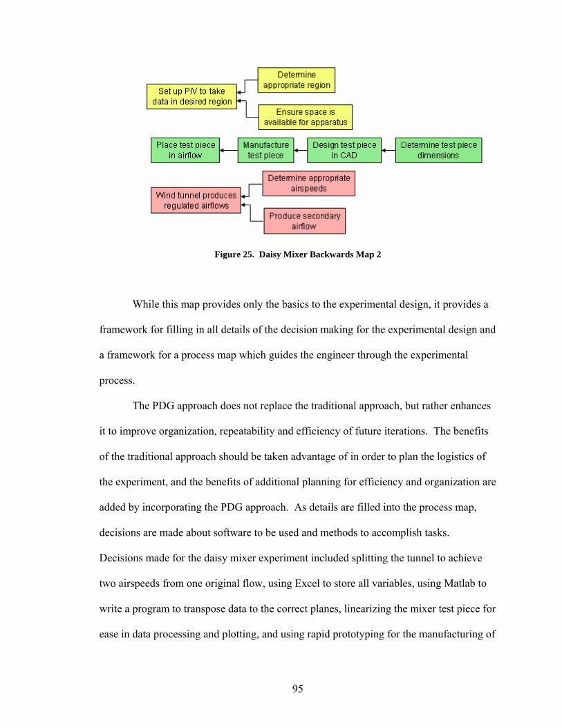
Figure 25. Daisy Mixer Backwards Map 2 While this map provides only the basics to the experimental design, it provides a
framework for filling in all details of the decision making for the experimental design and
a framework for a process map which guides the engineer through the experimental
process.
The PDG approach does not replace the traditional approach, but rather enhances
it to improve organization, repeatability and efficiency of future iterations. The benefits
of the traditional approach should be taken advantage of in order to plan the logistics of
the experiment, and the benefits of additional planning for efficiency and organization are
added by incorporating the PDG approach. As details are filled into the process map,
decisions are made about software to be used and methods to accomplish tasks.
Decisions made for the daisy mixer experiment included splitting the tunnel to achieve
two airspeeds from one original flow, using Excel to store all variables, using Matlab to
write a program to transpose data to the correct planes, linearizing the mixer test piece for
ease in data processing and plotting, and using rapid prototyping for the manufacturing of
95

the test piece. Figure 26 shows a detailed decomposition of the design process of the
daisy mixer experiment.
The completion of the first step of the PDG approach aids in the organization and
development of relationships, which is the second step of the PDG approach. The
schematic diagram of maps and sets shown in Figure 23 is used. Beginning with the end
in mind, maps and sets are populated until a complete architecture and organization
describe the experiment and a second iteration could be carried out by simply changing a
set of parameters and following the steps outlined. The main PDG structures the design
of the daisy mixer to be mounted to a turbine engine. The physical behavior is unknown
at this stage and the set B is desired. A predictive model does not exist and therefore the
predictive map P in the overall PDG must be substituted with an empirical process. The
sub-PDG structures the empirical process and is inserted into the main PDG, and the
deliverables set Ue becomes equal to the set B. Ue must contain data relating geometry to
vorticity. This set will become populated once two or more iterations of the experiment
have been conducted and a trend can be seen relating vortex magnitude and location to
particular geometry. Te contains the vorticity results of one iteration. Ie is the testing
procedure and maps the artifacts into Te. Ie contains models and procedures used in the
test itself, including PIV data processing and post processing software models. Ae
contains the solid model of the test piece, the test piece hardware, test instructions, the
rapid prototype build model, finishing instructions, a model showing the test set-up and
component placement, and testing procedure instructions. Ge contains parametric solid
model(s) of the test piece, parametric manufacturing models and documents such as the
rapid prototype model and finishing instructions, parametric models showing the test set-
96

Figu
re 2
6. D
etai
led
Map
of D
aisy
Mix
er D
esig
n Pr
oces
s
97

up and component placement, and a parametric document of testing procedure
instructions. Ae and Ge seem similar, however the difference is that Ae contains
instantiations of Ge, and Ge, as a map, contains parametric models and documents. The
master parameter list Me contains all the parameters needed for every model and
document contained in the maps Ge and Ie. Ce contains the customer requirements
vorticity and small lobe radius. De maps the customer requirements found in Ce to Me
and cannot be formulated until trends from the test results appear. The results from Te
will be compared to Ce so that De can be updated. The parameters found in Ce will
determine several parameters found in Me. Re contains the rules to map remaining
parameters found in Ke to Me. Ve will contain a record of all the parameters that went
into every model, which is an instantiation of Me. It will also contain every component
of Ae. Ee as the selection procedure in this case simply specifies that all of Me and all of
Ae are to be vaulted. Se takes all the results from Te and compiles them into a usable
format showing patterns of data. Figure 27 shows the members of the maps and sets for
the daisy mixer experiment.
Once the first two steps of the PDG approach are completed, the process is natural
to identify and implement process and task reuse. The nature of determining the maps in
the second step of the PDG approach encourages the engineer to plan the elements of the
experiment in a parametric manner. The reusable process is written in a PowerPoint
presentation (see Appendix) where the user can complete the steps outlined on a slide,
and easily click on a button to progress to the next step, navigating to choices of general
or detailed process steps and instructions. The process steps are organized into separate.
series of slides that can be followed in a different order if the nature of the experiment
98

Figure 27. Daisy Mixer Maps & Sets Schematic
changes. The user would simply set up the navigation in a different order if such were
the case. The process also refers to parameters that are stored and reused within a
spreadsheet as shown in Figure 28. In this way second and third iterations can be based
off of parameters identified during the first iteration. Reusable tasks within the process
include a parametric solid model which can produce a completely different model by
changing two or three key parameters, logic tables which determine the best wind tunnel
carrier frequency to use for different ranges of Hz input or camera placement for different
types of experiments, and a simple parametric model showing PIV traverse placement
measured from commonly used surfaces.
99

Figure 28. Daisy Mixer Parameter List Sample The benefit of the PDG approach is seen in the reduced number of steps and
reduced time required for specific steps during the second iteration of the experiment.
During the manufacturing of the test piece, 16 hours was reduced to .25 hours by using a
reusable parametric CAD model. Here it is observed that the same advantages that apply
to the complete product development cycle also apply to the empirical sub-cycle because
the empirical sub-cycle is a product development cycle in itself. The organization of all
parameters in one master parameter list using the PDG approach saved the engineer .25
hours of searching for the scaling factor which was found in the middle of a lab
notebook. The time saved while debugging the apparatus and test rig was a benefit of the
process map. A record of exact instructions which resulted in optimum reflection
blocking, camera calibration, and parameter optimization procedures saved 7 hours. For
example, photographs of optimum light placement during camera calibration resulted in
an excellent calibration after just one attempt. The traditional approach required much
time re-experimenting with light placement to satisfy what was termed “very finicky
software.” Photos of successful positions of black, laser blocking paper also saved much
time against one of the most difficult aspects of PIV use: the need to eliminate reflections
which corrupt data. The process map and handy location of parameters in the master
100

parameter list saved 4 hours of time using the PDG approach due mainly to good
organizational practices.
101

Chapter 6. Results and Conclusions
Although the amount of time saved by incorporating the PDG approach in the examples
presented was not on the order of weeks, months, or years, it is clear that these test cases
researched in this thesis are relatively simple compared to the types of experimental
testing that occurs in industry. The aerospace industry spends billions of dollars every
year because of required certification, experimental and validation testing processes.
Saving even a fraction of a percent in time and money costs is extremely significant. In
addition, products must be tested before they are sold not only in the aeronautical
industry but also in automotive and consumer products industries. If it’s possible to save
even a fraction of a percent of the current time invested into empirical processes, the
ideas presented have great worth. However, the worth is much more than a fraction of a
percent.
This thesis offers several contributions to the efficiency of the empirical process.
The advantages of incorporating the PDG approach when conducting empirical processes
include the following:
• The roles of empirical product development sub-cycles in overall product
development are identified
• Modern techniques of reuse and standardization to increase the efficiency of
empirical cycles are applied
o A generalized process map for each type of empirical sub-cycle is defined
102

o Opportunities for reuse are identified and parametric techniques are
defined
o Integration strategies for each type of sub-cycle within the overall product
development cycle are defined
• Improvement in cycle time of the empirical process is demonstrated and improved
repeatability for subsequent design iterations
o Significant time is saved as soon as the second iteration is conducted
o The number of steps is reduced for each iteration after the first iteration
o The value of planning ahead is observed
It is observed that before the PDG approach is implemented into empirical
processes, the simple principle of planning ahead reduced process steps significantly.
Namely, case 1 demonstrated that planning ahead reduced an empirical process from 28
to 24 steps. The true value of this thesis is seen when planning ahead is coupled with
PDG approach. The case studies demonstrate the clear advantages of using the PDG
approach in empirical processes: namely, incorporating principles of parametrics,
designing physical and mathematical models for reuse and parametric mapping into
empirical processes. Numbers of steps in the empirical process are reduced significantly
from 21%- 43% in the examples investigated, and actual time saved is believed to be
much greater although not measured specifically. Incorporating parametric models and
building reusable models eliminate a significant number of steps and replace them with
single button clicks, while process mapping not only eliminates some steps but also
reduces wasted time rethinking the process in order to conduct a feasible test or to
103
maintain consistent testing techniques to ensure accuracy of results. While planning or
re-planning an empirical process, there are two types of reuse to investigate: 1) reuse
within mathematical models, and 2) reuse of the fixtures and apparatus used for
conducting the tests. Process mapping can take place simply on a piece of paper or can
be incorporated into complex software to quickly guide the engineer through a process.
The conclusions for efficiency reached above do not even take into consideration
that a new person unfamiliar with specific procedures and process steps may often
conduct the second iteration of an empirical process. Significant time is lost while the
new engineer goes through the learning curve, rethinking what the testing process should
be. Complex tests where the same person conducts consecutive iterations also lose
efficiency due to the imperfection of the human mind to remember all process steps
perfectly. The PDG approach to empirical processes reduces and can eliminate these
losses of efficiency.
Finally, the small investment of an additional 10% of time in the first iteration of
an empirical process in order to incorporate PDG principles of thorough documentation,
parametrics, reusable models, and process mapping pays a generous return when the
second iteration alone can save several times that 10% investment.
104

105
References
1) Otto, K., Wood, K., Product Design, Prentice-Hall Inc., New Jersey, 2001
2) Ullman, D.G., The Mechanical Design Process, McGraw-Hill Higher Education, 2003
3) Doebelin, E.O., 1995, ENGINEERING EXPERIMENTATION: Planning, Execution, Reporting, McGraw-Hill, Inc., New York
4) Ingle, K.A., 1994, Reverse Engineering, McGraw-Hill, Inc., New York
5) Weber, C., Werner, H., Deubel, T., 2003, “A different view on Product Data Management / Product Life-Cycle Management and its future potentials,” Journal of Engineering Design; Vol. 14 Issue 4, p447-464
6) Wheelwright, S. C., 1989, “Time to market in new product development,” ICL
Technical Journal (International Computers Limited), v 6, n 4, p 625-646
7) Cooper, R.G., 1994, “Third-Generation New Product Processes,” Journal of Product Innovation Management, Vol. 11, No. 1, pp. 3-14
8) Roach, G., 2003, THE PRODUCT DESIGN GENERATOR—A NEXT GENERATION APPROACH TO DETAILED DESIGN, Dissertation, Brigham Young University, Provo, UT
9) Jensen, C.G., Tucker, S.S., Jones, C.J., and Rohm, T., 2000, “Concurrent Engineering with Parametric Design,” Proceedings the Third World Congress on Intelligent Manufacturing Process & Systems, Cambridge, MA
10) Roller, D., 1994, “Foundation of Parametric Modeling,” Parametric and Variational Design, B.G. Teubner Stuttgart, Germany
11) Jensen, C.G., Tucker, S.S., Jones, C.L., and Rohm, T., 2000, “Parametric Engineering Design Tools and Applications,” Proceedings of the 2000 Design Engineering Technical Conferences, Baltimore, MD, DETC2000/DAC-14275.
12) Tucker, S.S., 2000, Parametric Application Program Interface Function Mapping of Computer-Aided Design Systems, Masters Thesis, Brigham Young University, Provo, UT
106

13) Rohm, T., 2001, Graphical Creation of CAD Parametric Application Programs, Masters Thesis, Brigham Young University, Provo, UT
14) Jones, C.L, 2001, Parametric Model Behavior Across Multiple CAD Systems, Masters Thesis, Brigham Young University, Provo, UT
15) Engelbrektsson, P., Soderman, M., 2004, “The use and perception of methods and
product representations in product development: a survey of Swedish industry,” Journal of Engineering Design; Vol. 15 Issue 2, p141-154
16) Cyon Research, Sept 15, 2003, “The Road to the Future: How Product
Development Can Make the Journey More Profitable,” white paper
17) Yassine, A., Whitney, D., Daleiden, S., Lavine, J., 2003, “Connectivity maps: modeling and analysing relationships in product development processes,” Journal of Engineering Design; Vol. 14 Issue 3
18) Levardy, V., Hoppe, M., Browning, T. R., 2004, “Adaptive test process - An integrated modeling approach for test and design activities in the product development process”, Proceedings of the ASME Design Engineering Technical Conference, v 3, p 241-250
19) Schroeder, L. E., 2002, “Estimating Vehicle Interior Noise Using Room Models and Sound Power”, Sound and Vibration, v. 36 no7, p. 26-9
20) Kehrli, D. W., 1996, “Product development testing strategies,” Technical Papers, Regional Technical Conference - Society of Plastics Engineers, Basics to New Technologies, p F9-F14
21) Perkins, J. S., Kligerman, K. E., Knadle, K. T., Zubelewicz, A., 1996, “Innovative reliability tests as a means to shorten the product development cycle,” National Electronic Packaging and Production Conference-Proceedings of the Technical Program (West and East), v 3, p 1691-1699
22) Lu, Y., Loh, H. T., Brombacher, A. C., den Ouden, E., 2000, “Accelerated stress testing in a time-driven product development process,” International Journal of Production Economics, v 67, n 1, p 17-26
23) Ray, M. S., 1988, Engineering Experimentation, Ideas, Techniques and Presentation, McGraw-Hill Book Company, London
24) Grove, D. M., Davis, T. P., 1992, Engineering Quality & Experimental Design, John Wiley & Sons, New York
25) Funkenbusch, P. F., 2005, Practical Guide to Designed Experiments, A Unified Modular Approach, Marcel Dekker, New York
107

26) Wheeler, A. J., Ganji, A. R., 1996, Introduction to Engineering Experimentation, Prentice Hall, New Jersey
27) Ulrich, K.T, and Eppinger, S.D., 1995, “Product Design and Development”, McGraw-Hill, Inc., New York, 1995
28) Bare, M. and Klaass, R.M. Fred; “Improving CFD Modeling Using Rapid Prototype Testing”, SAE Power System Conference, 2004, paper no. 2004-01-3195
29) Roach, G.M., Cox, J.J., and Sorensen, C.D.; “The Product Design Generator: a system for producing design variants”, International Journal of Mass Customization, Vol 1, No. 1, 2005, p 83-106.
30) Teare, S., 2000, A Procedure Fore Structuring Product Information For Reusability, Masters Thesis, Brigham Young University, Provo, UT
108
Appendix
The reusable process described in Chapter 5 is written in the following PowerPoint
presentation where the user can complete the steps outlined on a slide, and easily
click on a button to progress to the next step, navigating to choices of general or
detailed process steps and instructions. The process steps are organized into separate
series of slides that can be followed in a different order if the nature of the experiment
changes. The user would simply set up the navigation in a different order if such
were the case. The process also refers to parameters that are stored and reused within
a spreadsheet as shown in Figure 28.
109

Figu
re A
1. P
IV D
ocum
enta
tion
Slid
e 1
110

Figu
re A
2. P
IV D
ocum
enta
tion
Slid
e 2
111

Figu
re A
3. P
IV D
ocum
enta
tion
Slid
e 3
112

Figu
re A
4. P
IV D
ocum
enta
tion
Slid
e 4
113

Figu
re A
5. P
IV D
ocum
enta
tion
Slid
e 5
114
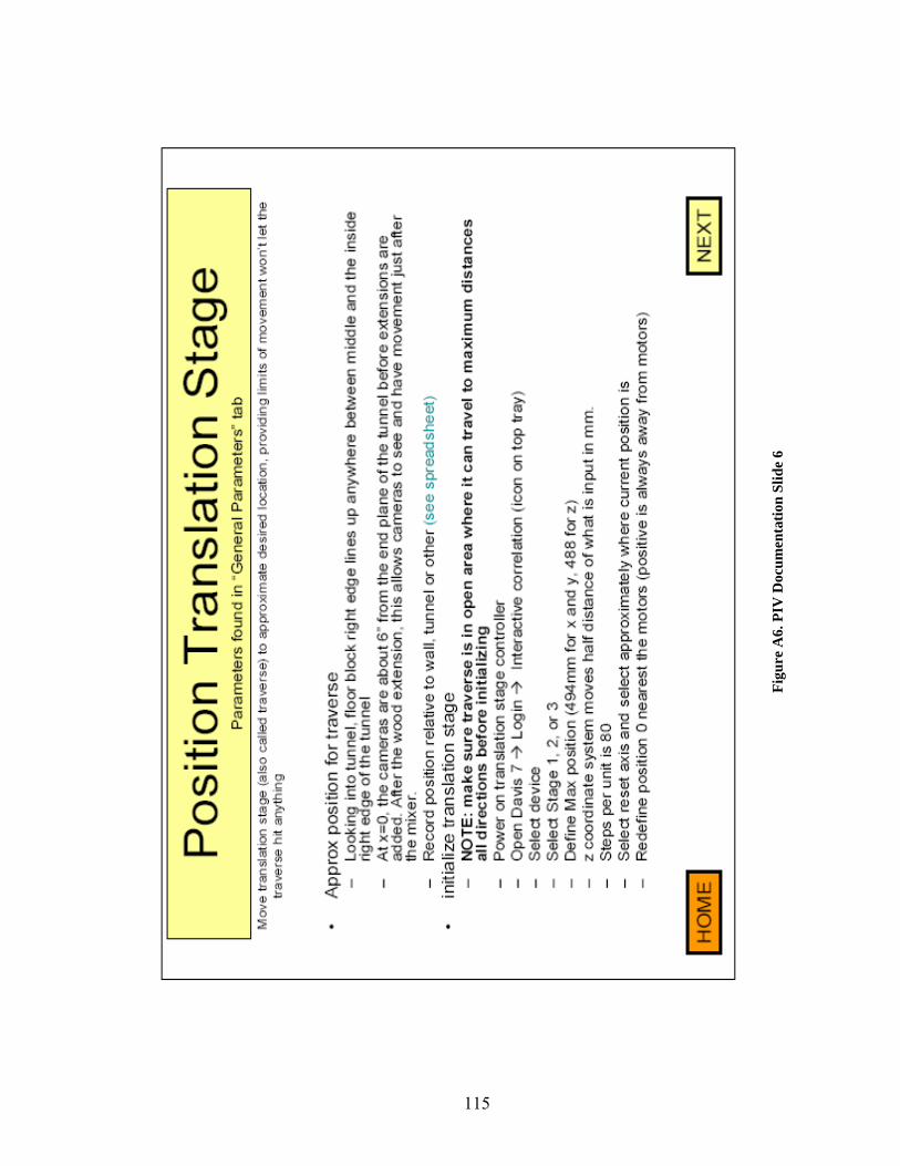
Figu
re A
6. P
IV D
ocum
enta
tion
Slid
e 6
115

Figu
re A
7. P
IV D
ocum
enta
tion
Slid
e 7
116

Figu
re A
8. P
IV D
ocum
enta
tion
Slid
e 8
117

Figu
re A
9. P
IV D
ocum
enta
tion
Slid
e 9
118

Figu
re A
10. P
IV D
ocum
enta
tion
Slid
e 10
119

Figu
re A
11. P
IV D
ocum
enta
tion
Slid
e 11
120

Figu
re A
12. P
IV D
ocum
enta
tion
Slid
e 12
121

Figu
re A
13. P
IV D
ocum
enta
tion
Slid
e 13
122

Figu
re A
14. P
IV D
ocum
enta
tion
Slid
e 14
123

Figu
re A
15. P
IV D
ocum
enta
tion
Slid
e 15
124

Figu
re A
16. P
IV D
ocum
enta
tion
Slid
e 16
125

Figu
re A
17. P
IV D
ocum
enta
tion
Slid
e 17
126

Figu
re A
18. P
IV D
ocum
enta
tion
Slid
e 18
127

Figu
re A
19. P
IV D
ocum
enta
tion
Slid
e 19
128

Figu
re A
20. P
IV D
ocum
enta
tion
Slid
e 20
129

Figu
re A
21. P
IV D
ocum
enta
tion
Slid
e 21
130
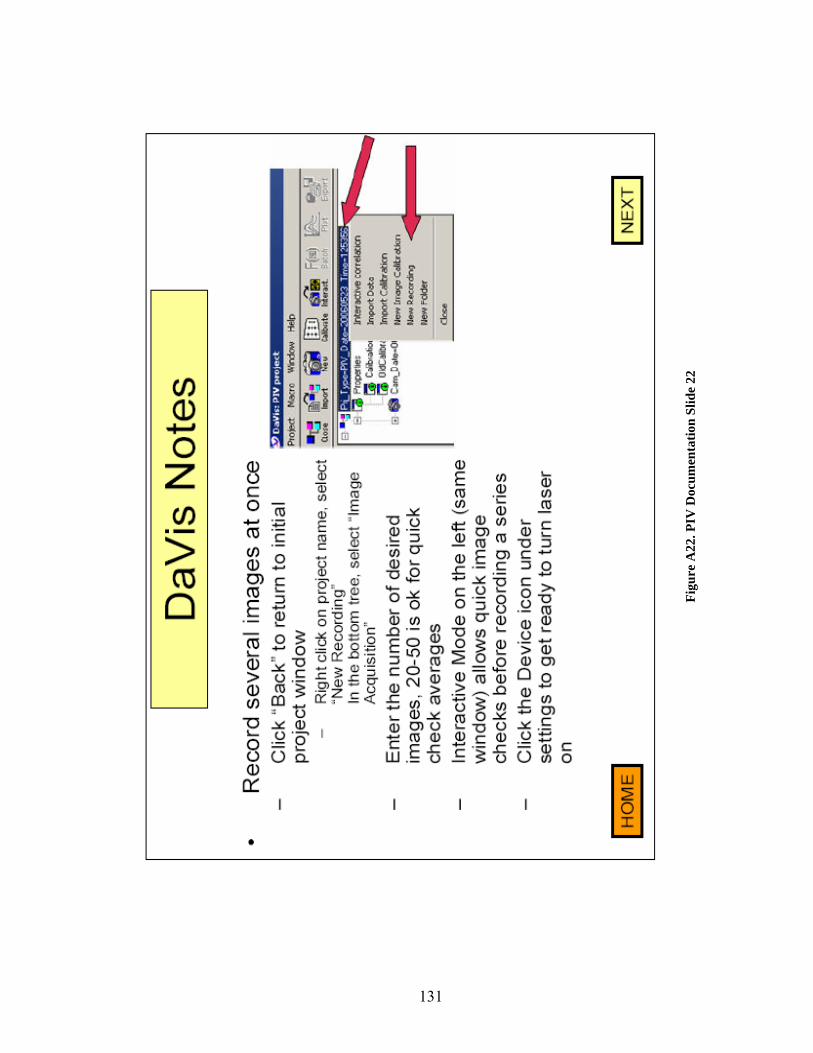
Figu
re A
22. P
IV D
ocum
enta
tion
Slid
e 22
131

Figu
re A
23. P
IV D
ocum
enta
tion
Slid
e 23
132

Figu
re A
24. P
IV D
ocum
enta
tion
Slid
e 24
133

Figu
re A
25. P
IV D
ocum
enta
tion
Slid
e 25
134


