

STUDY OF THE ANTAGONISTIC STIFFNESS OF PARALLEL
MANIPULATORS WITH ACTUATION REDUNDANCY
DIMITAR CHAKAROV
Institute of Mechanics, Bulgarian Academy of Sciences,
Block 4, Acad.G.Bonchev Street, 1113 Sofia, Bulgaria
Tel.: +359-2-7335216; Fax.: +359-2-8707498; E-mail: [email protected]
Abstract- In this paper parallel manipulators, consisting of a basic antropomorph kinematic
chain and parallel chains with redundant in number linear actuators are investigated.
Antagonistic stiffness, as a result of the actuation redundancy is also studied. A kinematic model
of parallel manipulators and a stiffness model are created. Conditions for specification of the
antagonistic stiffness are considered and the possibilities for generation of a desired stiffness
matrix are investigated. Approaches for specification of a desired compliance along a given
direction in the operation space and for specification of the biggest compliance in the operation
space are proposed. A scheme for stiffness control of manipulators with actuation redundancy is
developed on the basis of the above cited approaches. Computer experiments are performed and
a graphic interpretation of the results is presented.
Keywords- robot, manipulator, parallel, actuation, redundancy, antagonistic, stiffness, control,
compliance.
1.INTRODUCTION.
To execute high-value added operations, such as fine motion control and force control in assembly,
deburring, and many other manufacture tasks, one needs to design control strategies which would provide
accurate and stable motion. One of the natural solutions of these tasks is to incorporate into the robot
manipulator inputs whose number is larger than the needed minimum. If a manipulator possesses degrees of
mobility that outnumber the dimensions of the task space, the redundancy thus obtained is called “kinematic

redundancy”. On the other hand, if the number of the actuators is larger than that of the degrees of mobility,
the resulting redundancy is called “actuation redundancy” [1].
Additional degrees of mobility allow the realization of gross motion, dexterity, obstacle avoidance, etc.
Additional actuators significantly enhance the load handling capacity of the manipulator. However, actuation
redundancy is used to minimize joint torques or to satisfy actuator constrains [2],[3],[4]. At the same time, it
enables the system to modulate the end-effector stiffness by realizing an internal load distribution [5], [6],[7].
Parallel manipulators [8],[9] are designed with actuation redundancy, while kinematic redundancy is a
characteristic for serial manipulators. Parallel structures are created also by serial manipulators contacting the
environment, walking machines, multi-fingered end-effectors or coordinated multiple manipulators [10]. The
hybrid (serial-parallel) manipulators combine the properties of both types and admit kinematic, as well as,
actuation redundancy.
The hybrid manipulators with an anthropomorphic serial kinematic chain and with actuation chains, fixed
parallel to the serial one, copy to a certain extent the structure and actuation of the human limb. It is known
that the human limb is characterized by both kinematic and actuation redundancy. Thus, the human body
admits gross and dexterity motion, and at the same time undergoes large loads and has variable stiffness.
Purposeful motion under external mechanical disturbances and in the absence of any offered feedback is
executed in human and in animal natural limb[11]. This motion is possible because a given level of co-
activation of antagonistic muscles defines an equilibrium condition of the joint. Furthermore deviation of the
limb from this equilibrium state results in the generation of a restoring torque which is a function of the
mechanical properties of the muscle and is independent of other feedback. The shift to the next equilibrium
position is linked with the specification of a new appropriate set of muscle activities, required to define the
new equilibrium position. Moreover, it enables the inherent mechanical properties of the muscle-skeletal
systems to take care of the details of motion.
Similarly, the provision of an appropriate stiffness or compliance in an industrial manipulator considerably
simplifies tasks, involving manipulation of objects against kinematic constraints such as, for instance, the
insertion of a shaft into a bearing . Manipulation against kinematic constraints will be considerably simplified
if it is possible to specify motion of the end effector in response to arbitrary disturbance forces. Control
strategies, most generally known as stiffness control by redundant actuation [12], are developed for this
purpose. The strategies are part of impedance control schemes [13] where one can directly follow the ratio

“force-displacement”, and not each quantity separately. These considerations imply the necessity to describe
the desired dynamic relationship between the end-effector force and position.
Stiffness control schemes realized by employing redundant actuation are basically divided into: passive
stiffness control, feedback stiffness control, and stiffness control realized by means of antagonistic actuation.
First, the passive stiffness control is not exactly “control” but rather an analysis of the end-effector
characteristics, taking into account the stiffness of the system elements. The end-effector stiffness is a result of
the transformation of the joint stiffness and of the additional compliant elements introduced into the
manipulator structure [14], [15]. For example, such a scheme is used in the design of remote center compliance
(RCC) devices for assembly [16].
Second, feedback stiffness control is a scheme where the characteristics of the end-effector stiffness are
controlled by choosing proportional coefficients in the positioning joint controllers that would correspond to
the desired characteristics. An example of the development of such a scheme is the so-called “direct
compliance control (DCC)”, [17], [18]. One of the important features of such a control law is that the desired
arm dynamics is based on the stiffness parameters defined in the operation space. One can obtain the latter by
individually adjusting the stiffness parameters of each joint. One can also formulate the DCC law by analyzing
the relationship between the arm stiffness parameters defined in the operational space and those of the
actuation joint. One can obtain more compliance adjustable joints by using actuation redundancy. A
disadvantage of such a scheme, however, is the occurrence of constraints of the feedback control, on the one
hand, and the existence of stabilization problems, on the other hand.
Third, antagonistic actuation stiffness control uses a specific characteristic consisting in of the fact that the
actuation redundancy yields antagonistic forces in the mechanism. The internal forces balance each other in a
closed mechanism and do not perform any effective work but generate end-effector stiffness [5]. The following
solutions of the present scheme are known: open-loop stiffness control[12]; stiffness control which utilizes the
internal forces to modulate the stiffness at variable contact locations[19], and lower bound stiffness
control[20].
Open-loop stiffness control scheme introduces a feed-forward stiffness controller to alleviate the feedback
burden [12]. The open-loop stiffness control involves off-line planning of antagonistic actuator loads, such that
one can obtain the characteristics of the desired object stiffness, as well as the desired net effective load acting
on the object. Open-loop stiffness planning produce restoring forces against position disturbances or offsets.
Small perturbations or non-modeled dynamics remain to be compensated by the feedback controller.
A further continuation of [12] is the next scheme which utilizes the internal forces to modulate the
stiffness at variable contact locations on the object held by dual arm robots [19]. Except for a positioning
feedback controller, the scheme includes a stiffness controller with feedback with respect to position. The
required internal forces, that keep the contact stiffness close to the desired stiffness, can be determined by
minimizing an objective function with respect to the magnitude of the internal force.
Another control scheme [20] employs antagonistic actuation of three actuated legs and guarantees a lower
bound of the stiffness in all directions within the two dimensional task space. The control of the smallest
singular value of the end-effector stiffness guarantees the stiffness lower bound. Here, similarly to the previous
scheme, the stiffness model improves when applying feedback with respect to position.
The objective of the up-to-date work of the author is the investigation of parallel manipulators with
actuation redundancy. A procedure for structural and geometric synthesis of parallel manipulators with linear
drive modules is developed [21]. Investigations of the passive compliance of these manipulators are performed
[22]. The influence of the joint stiffness is shown considering the manipulator structure and position over the
end-effector stiffness variation.
The objective of the present work is to investigate the antagonistic stiffness produced by actuation
redundancy and to create an approach for specification of a desired stiffness in the operation space by means of
a magnitude variation of the antagonistic drive forces, suitable for a redundant manipulators control.
This paper is structured in the following way. Chapter 2 presents a kinematic model of the parallel
manipulators with a basic chain and a redundant number of parallel drive chains. Chapter 3 develops a model
of the end-effector stiffness, considering the stiffness and forces in the drive joints. Chapter 4 reveals the
conditions for specification of desired end effector stiffness. Chapter 5 presents some approaches for
specification of the stiffness and manipulator control. Conclusions are made in chapter 6.
2. A KINEMATIC MODEL OF PARALLEL MANIPULATORS.
The studied manipulators[21] presented in Fig.1. have a basic kinematic chain including the immovable
base 0 and two movable links connected by means of two rotational joints. The class of the kinematic joints is
not shown in Fig.1. The choice of rotational joints of class 3, 4 or 5 determines the number of degrees of
mobility of the basic chain. The manipulator end-effector is situated in the last link 2 of this chain, which

moves in a ν-dimensional operation space. Parallel kinematic chains - m in number are attached to the
immovable basis and to the links of the basic chain. These chains consist of similar type drive modules with
one single drive joint for a linear motion P and two passive rotational joints R1 and R2. The number of the
degrees of freedom of each parallel chain is equal to three in the planar case and to six in the spatial one. In
this way the number of the manipulator degrees of mobility is defined by the number of the degrees of
mobility of the basic chain h. The number of degrees of mobility of the studied manipulators with actuation
redundancy h should be less than the number of the drive modules m ( h<m ).
The parameters of the relative motion in the drive linear joints of the parallel chains are sellected as
generalized parameters for the kinematic system definition:
λ = [λ1, ….., λm]T (1)
and the parameters of the relative motion in the joints of the basic chain
q = [q1, …., qh]T . (2)
Every closed loop in the parallel manipulator structure produces links between the generalized parameters
(1) and (2). These links can be defined by means of the vector function
(3) ( )qΦλ =
which allows to calculate the parameters (1) from parameters (2).
Part of the parameters (1) with number h
[ Th1 ,...,λλ=uλ ]
]
(4)
which are sufficient for the kinematic system definition are called independent parameters, and the remaining
part of the parameters with number (m-h)
[ Tm1hd λ,...,λ +=λ (5)
are called dependent parameters. Then vector (1) has the representation:
λ = [λu ; λd]T. (6)
The differentiation of (3) with respect to time is:
(7) qLλ && =
and defines (m x h) matrix of the first partial derivatives:
[ Tdu L;L
qλL =⎥⎦
⎤⎢⎣
⎡∂∂
= ] (8)
comprising of (h x h) matrix
⎥⎥⎦
⎤
⎢⎢⎣
⎡
∂∂
=qλ
L uu (9)
And (m-h)xh matrix
⎥⎥⎦
⎤
⎢⎢⎣
⎡
∂∂
=qλ
L dd (10)
The matrix of the partial derivatives of the dependent parameters (5) with respect to the independent (4) is
defined with the help of (9) and (10)
[ 1ud
u
d LLλλ −=⎥
⎦
⎤⎢⎣
⎡∂∂ ], (11)
and the matrix of the partial derivatives of all the parameters in the drive joints (1) with respect to the
independent parameters (4) is defined as
⎥⎦
⎤⎢⎣
⎡=⎥
⎦
⎤⎢⎣
⎡∂∂
−1udu LL
Eλλ (12)
where E is the unity (h x h) matrix.
The double differentiation of (3)
qHqqLλ T &&&&&& += (13)
produces (m x h x h) matrix of the second order partial derivatives
[ Tdu H,H
qLH =⎥⎦
⎤⎢⎣
⎡∂∂
= ] (14)
Each plane of (14), Hi, i=1,....,m is a (h x h) matrix with elements:
⎟⎟⎠
⎞⎜⎜⎝
⎛
∂∂
∂∂
=∂∂
∂=
j
i
kjk
i2
kj,i, qλ
qqqλ
H j = 1, …, h; k = 1, ..., h (15)
The link between the parameters of the basic chain (2) and the end-effector co-ordinates
(16) [ ] 6,T ≤ν= ν1 X,...,XX
is defined by means of the direct problem of the kinematics of the serial manipulators. This problem on the
level of displacements, velocities and accelerations is presented by means of the equations:
(17) Ψ(q)X =
(18) qJX && =
(19) qGqqJX T &&&&&& +=

where:
⎥⎦
⎤⎢⎣
⎡∂∂
=qXJ (20)
is the (νx h) matrix of Jacoby
and ⎥⎦
⎤⎢⎣
⎡∂∂
=qJG (21)
is the (νx h x h) matrix of the second order partial derivatives.
3. STIFFNESS MODEL AT REDUNDANT ACTUATION.
The manipulation system which is in contact with the environment is considered to be in a static balance
without consideration of the gravitation forces.
We can define the driving forces in the linear joints of the parallel chains with:
(22) [ Tdu F;FF = ]
]
]
]
]
where and are vectors of the driving forces corresponding to the independent parameters (4) and the
dependent parameters (5). The forces:
uF dF
[ Th1u F,...,F=F (23)
are sufficient for the manipulator motion along a given trajectory and are considered as basic forces, while the
forces:
[ Tm1hd F,...,F +=F (24)
are considered as additional driving forces.
The effective generalized forces in the linear joints corresponding to the independent parameters (4) can be
defined by means of the (h x 1) vector:
[ (25) Th1,...,UU=U
The effective generalized torques in the joints in the basic serial chain corresponding to the parameters (2)
can be defined by means of the (h x 1) vector:
(26) [ Th1,...,QQ=Q
The external forces and torques applied at the end effector and corresponding to the co-ordinates (17) can
be defined by means of the (ν x 1) vector:

, ν ≤ 6 (27) [ T1 P,...,P ν=P ]
The relations between the forces cited above can be defined according to the principle of the virtual
work. In this way, from equation (12) follows the relation between the driving forces (22) and the effective
generalized forces (25):
(28) FLLЕ
UТ
1ud⎥⎦
⎤⎢⎣
⎡= −
or (29) [ ] dТ1
udu FLLFU −+=
The relation between the effective generalized forces (25) in the linear joints and the generalized effective
torques (26) in the joints of the basic chain can be defined with the help of (9):
(30) ULQ Tu=
And considering (28) we can define the equation:
(31) FLQ T=
The link between the external forces and torques (27) and the effective generalized torques (26) can be
defined using (20):
(32) PJQ T=
The last three equations (30), (31) and (32) define the link between the external and driving forces, on the
one hand:
FLPJ TT = (33)
and the link between the external and the effective generalized forces, on the other hand:
(34) ULPJ Tu
T =
Differentiation of (33) with respect to parameters (2) produces the equation:
qFLF
qL
qPJP
qJ T
TT
T
∂∂
+∂∂
=∂∂
+∂∂ (35)
This after consideration of (21), (20), as well as (14), (8), can be expressed:
LFLFHJXPJPG TTTT
λ∂∂
+=∂∂
+ (36)
The equation above defines the manipulator as an elastic system in which the end-effector stiffness
XPК
∂∂
= (37)

is defined by the axes stiffness in the linear drive joints
λ∂∂
=FK sh (38)
and the latent stiffness described by the expressions and PG T FH T . The latent stiffness is a result of the
static equilibrium in the contact process (33) between the external forces (27) and the driving forces (22) on
the one hand, and a result of the balance (29) between the basic and the additional driving forces (23) and (24),
on the other hand, with consideration of the contact condition
(39) dTd
Tuu FLLUF −−=
The generated stiffness, as a result of the antagonistic force equilibrium is called antagonistic stiffness.
The equality (36) can be defined as follows, using (37), (38), (14), (22), (39) and (34):
LKLFHFLLHKJJPGPJLH shT
dTdd
Td
Tu
Tu
TTTTu
Tu ++−=++− −− (40)
Actuation redundant manipulators allow specification of the end-effector stiffness by distribution of the
magnitudes of the additional driving forces (24) according to the equation (40).
It is convenient in the process of simulations and control to use the reverse stiffness matrix (37):
1−= KB (41)
called the compliance matrix of the end-effector.
The compliance of the end-effector which is specified in the process of control is investigated without
consideration of the external forces. According to (40) and (41) and P = 0 the end-effector compliance
defined in the operation space can be expressed as :
(42) Tsh
Td
Tdd
Td
Tu
Tu J]LKLFHFLLH[JB 1−− ++−=
4. CONDITIONS FOR SPECIFICATION OF DESIRED END-EFFECTOR COMPLIANCE.
The stiffness control realization for control of manipulators with actuation redundancy is linked with
specification of a suitable end-effector stiffness or compliance. This stiffness is a reason for generation of
restoring forces, as an expected response of the external excitation in the contact process.
During the performance of feedback stiffness control [17], [18] the end-effector compliance (42) is
specified by means of stiffness selection in the drive joints (38). The compliance (42) is specified by proper
selection of the magnitudes of the additional driving forces (24) in the realization of antagonistic actuation
stiffness control [12], [19], [20]. It is necessary that the partial derivative matrixes J, L and H not to be

singular in the process of stiffness specification [9]. Also, it has to be considered that the symmetric
compliance matrix (41) is positively defined and also with positive eigen values or
0>Bdet и bii>0 (43)
where bii are the diagonal matrix components.
The symmetrical compliance (ν x ν) matrix (41) has µ=νx(ν+1)/2 independent components. The
manipulator must have µ in number additional driving joints theoretically, for the full compliance matrix
specification according to equation (42). Each drive joint is considered a generator either of shaft stiffness
(element of Ksh) or of an antagonistic acting force (element of Fd) [22]. The general number of the drive joints
must be µ+h because for the manipulator motion control with h degree of mobility are necessary h in number
drive joints. The parallel manipulator must posses m= µ+h in number parallel chains if every parallel chain
possesses one drive joint.
The desired end-effector compliance can be represented by vector
(44) [ Tj1
0 b,...,b,...,b µ=b ]
including the independent components of the matrix (41) and can be specified by calculation of µ in number
suitable components of the diagonal matrix of the shaft stiffness (38) united in the vector
[ ]Tshshsh k,...,k1 µ
=k (45)
This can be performed by solving a system of linear equations derived from (42);
( )( )( )sh
sh
sh
kkk
µµ
jj
11
fbfbfb
===
(46)
The obtained system solutions may contain though, extremely high or negative values of the investigated
joint stiffness. This is the reason why serious stabilization problems are created in the manipulator control
[18]. As a result, the application of this approach is restricted.
The desired compliance (44) can be specified also by µ in number components of the vector of the
additional driving forces (24). In this case the system of linear equations derived from (42) is:
( )( )( )d
d
d
FFF
µµ
jj
11
fbfbfb
===
(47)
The upper system solutions can be derived using unrealistically high values of the driving forces (24). The
possibilities to find solutions of system (47) are narrowed due to the existence of practical restrictions in the

magnitudes of these forces. Solving the problem for specification of a given compliance using restricted
parameters can be performed by means of optimization [22]. In this case there are difficulties in defining the
real forces (24), which generate the compliance matrix satisfying limits (43).
Computer experiments are carried out in order to investigate the correlation of the generated compliance
with respect to inequality (43). The carried out experiments are two dimensional (2D), where the compliance
in the operation space is defined by a 2D linear compliance matrix.
, (48) ⎥⎥⎦
⎤
⎢⎢⎣
⎡=
yyxy
xyxxLbbbb
B
The next coefficient is derived on the basis of (43) for the 2D case from (48):
yyxx
xy
bb
b=κ . (49)
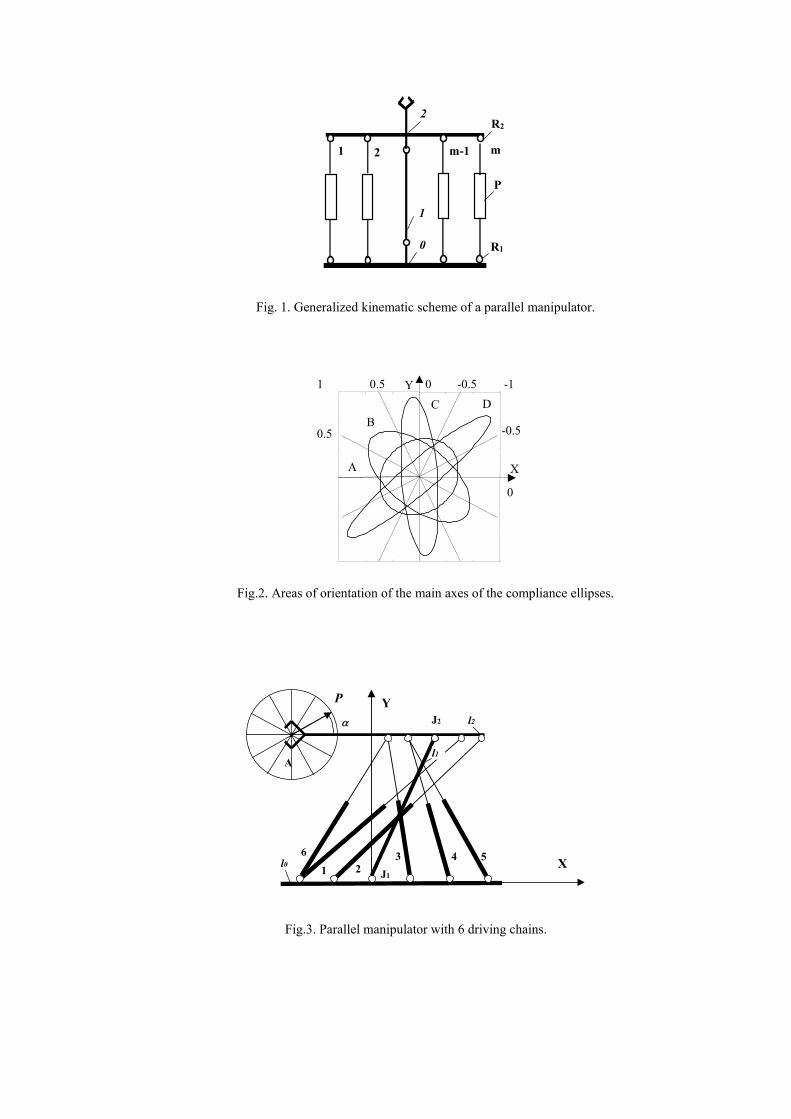
The values of this coefficient, which are among the limits –1<κ<1 define stiffness generation. Besides, this
coefficient can be used indirectly for qualitative evaluation of this stiffness. If compliance is represented in a
graphic way by means of compliance ellipse, the values of κ close to 1 define the biggest angle of deviation of
the main ellipse axes of the co-ordinate axes, while at κ=0 the ellipse axes coinside with the co-ordinate axes.
Four areas of orientation of the main compliance ellipse axes are formed for the generated stiffness evaluation
assigned with A, B, C, D as shown in Fig.2. The four areas are identified by means of the coefficient
magnitude (49) and the relation of the elements bxx and byy as cited below:
A: and b5.05.0 ≤κ≤− xx< byy (50)
B: 15.0 ≤κ≤
C: and b5.05.0 ≤κ≤− xx> byy
D: 5.01 ≤κ≤−
The experiments are performed using a 2D parallel manipulator shown in Fig.3. The manipulator consists
of a basic chain with one immovable and two movable links l0, l1, l2 (l1=l2=0.4 [m]) linked by means of two
rotational joints J1 и J2 (h=2). The manipulator can include in the structure from 1 to 6 in number parallel
drive chains attached to the immovable base l0 and to link l2 as shown in the figure. The parallel chains are
shown in Fig.3 with numbers 1,2,3,4,5,6. The end-effector compliance is evaluated with a discrete variation of
the magnitudes and the direction of the driving forces in the limits:
, [N] (51) 6,...,3i,300F300 i =≤≤−

The stiffness generation is defined by the values of the coefficient (49), which are situated in the areas (50).
The stiffness generation at given force distribution is graphically interpreted by one of the signs
corresponding to the areas A, B, C, D. Several structural variants are considered varying
the number of the manipulator driving chains.
First of all a manipulator shown in Fig.3 with 4 parallel chains marked with 1, 2, 4 and 5 is considered.
Discrete values within the limits (51) are assigned to the additional forces Fd in two driving joints (4 and 5).
The experimental results are shown in the graphics in Fig. 4a. The values of the additional forces Fd4 и Fd5
are pointed out along the co-ordinate axes.
A solution of a variant of a manipulator with 5 parallel chains (1, 2, 3, 4, 5 in Fig.3.) is considered. The
additional driving forces Fd3, Fd4, Fd5 in the three joints 4, 5, 6 vary within the limits (51). Results for stiffness
generation are shown in Fig. 4b, where the same co-ordinate axes (Fd4 and Fd5) are used. There exist cases of
different orientation of the compliance ellipse axes for one value of the forces Fd4 and Fd5 on the graphics
shown in Fig. 4b, which are derived by variation of the third force Fd3.
A case study is performed when the manipulator is a variant with 5 parallel chains (1, 2, 3, 4, 5 in Fig.3.),
but the forces Fd4 and Fd5 vary within two of the joints (4, 5) and also the shaft stiffness ksh1 , ksh2 ksh3 vary in
the driving joints of the remaining chains (1, 2, 3). Discrete values are given to the stiffness within the limits:
[N/m] (52) 3,...,1i,500k0ish =≤≤
Graphic interpretation of the experimental results is shown in Fig.4c.
The last structural solution revealed is of a manipulator variant with 6 parallel chains (1, 2, 3, 4, 5, 6 in
Fig.3.). The forces Fd3, Fd4, Fd5, Fd6 receive discrete values within the limits (51). The results are shown in a
similar way in Fig. 4d.
The basic conclusions of the results of the carried out experiments are:
effect of the antagonistic stiffness does not exist for all values of the driving forces in spite of the
existence of an antagonistic equilibrium among them;
the possibility for orientation variation of the compliance ellipse axes by means of variation of the
magnitudes and orientations of the additional forces and the values of the shaft stiffnesses is limited.
increasing the number of the additional driving chains gives more possibilities for axes orientation
variation of the compliance ellipse and also widens the diapason in which the forces generate stiffness.
5. SOME APPROACHES FOR COMPLIANCE SPECIFICATION AND MANIPULATOR
CONTROL.
Specification of a random compliance matrix of a manipulator by means of antagonist driving forces
distribution is not always possible according to the cited above conditions. On the other hand the full
compliance matrix specification is not necessary for many case problems. For series technological tasks
specification is sufficient only for certain components of the compliance matrix or specification is enough only
along a single direction in the operation space or guaranteeing is needed for the upper compliance limits in the
operation space. Some approaches are developed for these reasons which do not include specification of the
full compliance matrix. The following optimization procedures are carried out for these approaches and
verified by computer experiments.
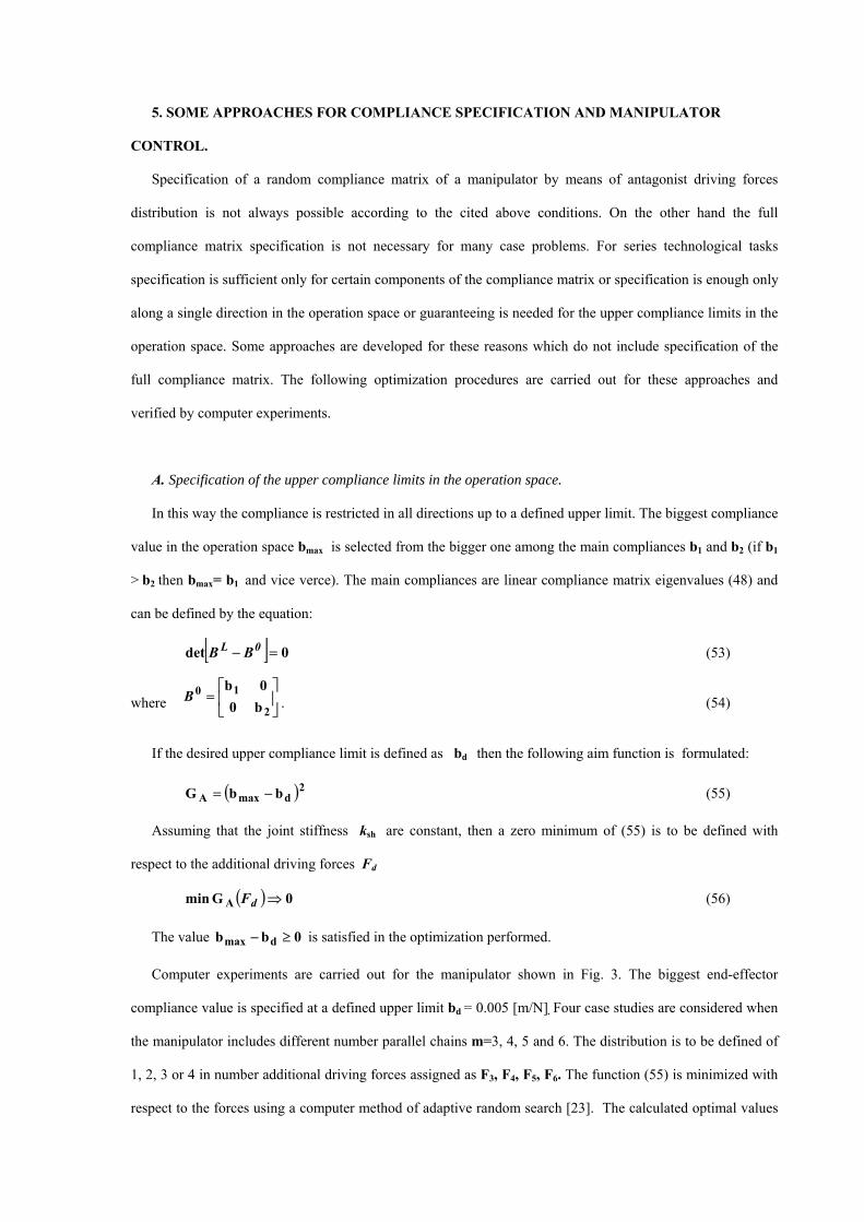
A. Specification of the upper compliance limits in the operation space.
In this way the compliance is restricted in all directions up to a defined upper limit. The biggest compliance
value in the operation space bmax is selected from the bigger one among the main compliances b1 and b2 (if b1
> b2 then bmax= b1 and vice verce). The main compliances are linear compliance matrix eigenvalues (48) and
can be defined by the equation:
[ ] 0det =− 0L BB (53)
where ⎥⎦
⎤⎢⎣
⎡=
2
10b00b
B . (54)
If the desired upper compliance limit is defined as bd then the following aim function is formulated:
(55) ( 2dmaxA bbG −= )
Assuming that the joint stiffness ksh are constant, then a zero minimum of (55) is to be defined with
respect to the additional driving forces Fd
(56) ( ) 0Gmin A ⇒dF
The value is satisfied in the optimization performed. 0bb dmax ≥−
Computer experiments are carried out for the manipulator shown in Fig. 3. The biggest end-effector
compliance value is specified at a defined upper limit bd = 0.005 [m/N]. Four case studies are considered when
the manipulator includes different number parallel chains m=3, 4, 5 and 6. The distribution is to be defined of
1, 2, 3 or 4 in number additional driving forces assigned as F3, F4, F5, F6. The function (55) is minimized with
respect to the forces using a computer method of adaptive random search [23]. The calculated optimal values

of the additional forces are cited in Table 1-a. In this table are shown the magnitudes of the forces F1 and F2
according (39) as well as the averaged value of all the forces marked with F. The ellipses of the generated
compliance are building up in Fig. 5. For each case marked with 1, 2, 3, and 4. In the same figure the circular
ellipse of the limit compliance marked with 5 (b1=b2= bd) is shown.
B. Compliance specification along a given direction in the operation space.
The desired direction in the 2D solution is defined by the unity vector:
(57) Tyx ]p;p[=P
where . 1=PP T
The compliance in the same direction is defined by the equation:
(58) PBP LT=Pb
where BL is the linear compliance matrix (48).
We suppose that the shaft stiffnesses in the joints ksh are constant in one position from the manipulator
trajectory q0 , so the compliance in the given direction P is defined by the magnitudes of the additional driving
forces Fd.
If we mark the desired compliance in the given direction with , then the following aim function can
be defined:
Pdb
(59) ( 2PdPB bbG −= )
]
and we are looking for a zero minimum of (59) with respect to the driving forces Fd
. (60) ( ) 0Gmin B ⇒dF
The value is satisfied in the optimization performed. 0bb PdP ≥−
The manipulator presented in Fig. 3. is used for the computer experiment utilizing the cited above
approach, including 6 parallel driving chains 1, 2, 3, 4, 5, 6. The magnitude of the desired compliance is
=0.005[m/N]. The following experiments are carried out. Pdb
First of all is specified the compliance in point A in the operational space (Fig. 3.) along several directions
defined by the vector (57):
, (61) [ Tsin;cos αα=P
where α = 300 ; 600; 900; 1200; 1500; 1800 for different directions.

The function (59) is minimized with respect to the forces F3, F4, F5, F6 using the same numerical method
[23]. The derived optimal magnitudes of the driving forces are shown in Table 1-b). In the same table are
shown the magnitudes of the forces F1 and F2 according to (39), as well as the averaged value of all the forces
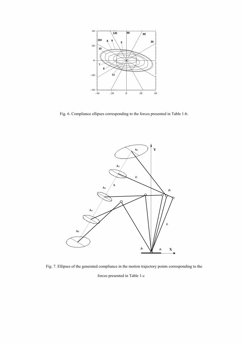
marked with F. In Fig. 6 are presented the directions of P and the compliance ellipses generated by the
antagonistic forces. Their intersection points correspond to the desired compliance , which in all directions
is represented with a circular ellipse marked with 5 (b
Pdb
1=b2= ). Pdb
In the next experiment the compliance in several points (А1, А2, А3, А4, А5 ) is specified from a single
trajectory S in the operation space as shown in Fig. 7. In each point the desired compliance =0.005[m/N]
is specified along a single direction defined by the vector (61) at α = 150
Pdb
0 . After minimization of (59) the
derived optimal values of the forces F3, F4, F5, F6 as well as the forces F1, F2 and F for each trajectory point
are presented in Table 1-c. In Fig. 7. is shown the compliance ellipse generated by these forces in the
corresponding points. The intersects of these ellipses along the given direction are presented corresponding to
the desired compliance.
The experiments performed show that the approaches accepted allow easy and effective definition of the
desired stiffness without full compliance matrix specification. The first approach is a more common one
restricting the compliance along all directions due to the higher driving forces values. The dimensions of these
forces is deminished at a higher drive number (Table 1-a). The second approach restricts the compliance only
along the given direction. The driving forces magnitude in this case depends to a great extend on the cellected
direction (Table 1-b). In this way in one direction (α=900 , Table 1-b) the driving forces magnitude and the
generated compliance type (curve 9 in Fig.6) coincides with the results of the first approach (curves 4 in
Fig.5). In another direction (α=1800, Table 1-b) the forces diminish several times, while the compliance along
the same direction approaches the minimal value Fig.6. We can perform generation of such compliance along
every direction by means of imposing additional criteria for optimization, which may coincides with the
minimal compliance value.
The compliance variation at manipulator position variation in the operation space can be corrected up till
desired magnitudes by using the cited approaches A and B. This can be performed for small values of the
antagonistic driving forces using the second approach (Fig.7.). The cited above experiments are carried out
using zero stiffness values in the joints (45). The estimation of the constant values of the joint stiffness in the
performed optimization results in deminishing the values of the necessary driving forces.

The studied approaches and the experiments performed for specification of a desired stiffness allow
creation of a redundant actuated manipulators control based on the antagonistic stiffness. An open loop
stiffness control scheme is developed and shown in Fig.8.
The scheme includes one feed forward stiffness controller where off-line can be planned the magnitudes of
the redundant drive forces Fd , generating the desired compliance bd along the desired trajectory points qd .
These forces can be defined by means of optimization using one of the cited approaches: A. Specification of
the highest compliance level, or B. Specification of the compliance along a certain direction. It is supposed
that the joint stiffness Ksh is maintained constant, when calculating the end effector compliance using (42). In
this controler the positions in the independent drive joints λud are also calculated following the values of the
desired trajectory qd by using equation (3).
The scheme includes one feed back controller where on-line is controlled the position in the independent
drive joints λu and the values of all the drive forces F. The optimal values of the additional drive forces Fd 0
which guarantee the desired compliance in a point of the defined trajectory and together with the outputs of the
position controlers in the independent joints U, form according to (39) the control influences in the
independent joints Fu0 . The full vector of the control influences F0 in the independent and in the dependent
driving joints which ensures motion along a desired trajectory and guarantees a desired compliance, is
implemented in the joint force controllers. The existing disturbance from the desired trajectory generates a
restoring force in opposite direction of the deviation. The magnitude of this force is defined not so much by the
magnitudes of the feed-back coefficients in the joint controlers but by the values of the given compliance.
6. CONCLUSION.
The developed in this work kinematic model of parallel manipulators and a stiffness model at actuation
redundancy are a basis for investigation on the mechanical properties of parallel manipulators and for
developing of control strategies. The presented investigations of the stiffness show that the existence of the
antagonist equilibrium is not always sufficient for specification of desired stiffness of the end-effector. The
possibilities for this effect are bigger with a higher number of the redundant actuators. Approaches which do
not require specification of the full compliance matrix are developed for solving this problem.Two approaches
are suggested for compliance specification along a certain direction in the operation space and for specification
of the highest compliance level in a point of the operation space. An open loop stiffness control scheme is
developed on the basis of the created approaches, including one feed forward stiffness controller, and one

feedback position controller. The investigations carried out on the antagonist stiffness can be used in industrial
manipulators fulfilling contact tasks where the generated antagonist stiffness gives the system response to the
arbitrary disturbance forces.
REFERENCES:
1. Bh. Dasgupta, and T.S.Mruthyunjaya, Forse Redundancy in Parallel Manipulators: Theoretical and
Practical Issues. Mech.and Mach.Theory, V.33, No6, (1998),727-742.
2. J.F. Gardner , V.Kumar, J.H.Ho, Kinemayics and Control of Redundantly Actuated Closed Chains. IEEE
Int. Conf.on Robot and Automation, Scottsdale, 1989, pp.418-424.
3. M.A. Nahon , J. Angeles, Forse Optimisation in Redundantly – Actuated Closed Kinematic Chains.
IEEE Int. Conf.on Robot and Automation, Scottsdale, 1989, pp.951-956.
4. S. Tadokoro., Control of Parallel Mechanisms. Advanced Robotics, Vol.8, No6, 1994, pp.559-571.
5. W. Cho, D. Tesar, R. Freeman, The Dynamic and Stiffness Modeling of General Robotic Manipulator
Systems with Antagonistic Actuation. IEEE Int. Conf. on Robot. and Autom., CH2750-8/89, (1989),
pp.1380 - 1387.
6. Byung-Ju Yi, R.Freeman, Geometric Characteristics of Antagonistic Stiffness in Redundantly Actuated
mechanisms. IEEE Int. Conf. on Robot and Automation, Atlanta, 1993, pp.654-661.
7. Byung-Ju Yi, Il Hong Suh, Sang-Rok Oh, Analysis of A 5-bar Finger Mechanism Having Redundant
Actuators with Applications to Stiffness. IEEE Int. Conf. on Robot and Autom., Albuquerque, 1997,
pp.759-765.
8. J.-P. Merlet, Les Robots paralleles. Hermes, Paris, 1990, p.1.
9. C. Gosselin, Stiffness Mapping for parallel Manipulators. IEEE Ttransactions on Robotics and
Automation, Vol.6, No.3, 1990, pp. 377-382.
10. T. Tarn, A.Bejczy and X.Yun, Design of Dynamic Control of Two Cooperating Robot Arms: Closed
Chain Formulation. IEEE Int.Conf. on Robot and Autom., CH2413-3-87, (1987), pp.7-13.
11. N. Hogan, Mechanical Impedance Control in Assistive Devices and Manipulators. Joint Autom. Control.
Conf. ,San Francico, Vol.1, 1980, pp.361-371.
12. Byung-Ji Yi, R.Freeman, D. Tesar, Open-Loop Stiffness Control of Overconstrained Mechanisms/Robotic
Linkage Systems. IEEE Int. Conf. On Robotics and Automation, Scottsdale,1989, pp.1340-1345.
13. N. Hogan, Impedance Control: An Approach to Manipulation , ASME J. Dynamic Systems Meas. &
Control., Vol.107, 1985, pp. 1-24.
14. J.K.Mils, Hybrid Actuator for Robot Manipulators: Design. Control and Performance. IEEE Int. Conf.. on
Robotics and Automation, Cincinati, 1990, pp.1872-1878.
15. S. Mittal, Uri Tasch, Yu Wang, A Redundant Actuation Scheme for Independent Modulations of Stiffness
and Position of a Robotic Joint. DSC-Vol.49, Advances in Robotics, Mechatronics and Haptic Interfaces,
ASME, (1993), 247-256
16. H. Lipkin, and T.Patterson. Generalized Center of Compliance and Stiffness. IEEE Int. Conf. on Robotics
and Automation, Nice, France, 1992, pp.1251-1256.
17. K. Yokoi, M. Kaneko, K.Tanie, Direct Compliance Control of Parallel Link Manipulators. “8th CISM -
IFToMM Symp.”Ro.man.sy’90”, Cracow , 1990, pp.224 - 251.
18. K. Yokoi, M. Kaneko, K.Tanie, Direct Compliance Control for a Parallel Link Arm (2nd Report - The
Stability Analysis for the Arm with Negative Stiffness Joints). Trans. Jpn. Soc. Mech. Eng.©,Vol.55,
No.515, 1989, pp.1690-1696.
19. M. Adli, K. Ito and H. Hanafusa, A method for modulating the contact compliance in objects held by dual-
arm robots. Int. Conf. on Recent Advances in Mechatronics, Istanbul, Turkey, 1995, pp.1065-1072.
20. S. Kock , W.Schumacher. A Parallel x-y Manipulator with Actuation Redundancy for High-Speed and
Active-Stiffness Applications. IEEE Int. Conf. on Robot and Autom., Leuven, Belgium, 1998, pp. 2295-
2300.
21. D. Chakarov and P. Parushev. Synthesis of Parallel Manipulators with Linear Drive Modules.
Mechanism and Mashine Theory, Vol.29, No.7, 1994, pp.917-932.
22. D. Chakarov, Study of the Passive Compliance of Parallel Manipulators. Mechanism and Machine
Theory, Vol.34, No3, 1999, pp.373-389.
23. I. Edisonov , Optimization Method Adaptive Random Search with Translating Intervals. American Jorn.
of Math. and Menag. Sc., Vol.14, No3&4, 1994, pp.143-166.
0
2
1
1 2 m-1 m
R1
R2
P
Fig. 1. Generalized kinematic scheme of a parallel manipulator.
0.51 0 -0.5 -1
X
0.5 -0.5
Y
0
A
BC D
Fig.2. Areas of orientation of the main axes of the compliance ellipses.
1 23 4 5
J1
J2
l1A
X
Y
6l0
P
l2α
Fig.3. Parallel manipulator with 6 driving chains.

a) Fd4 [N]
Fd5 [N]
b)Fd4 [N]
Fd5 [N]
c)
Fd5 [N]
Fd4 [N] d)
Fd4 [N]
Fd5 [N]
Fig. 4. Variation of the main axis orientation of the compliance ellipse.
512
3 4
Fig. 5. Compliance ellipses corresponding to the forces presented in Table 1-a.
598
10
76
11
60
30
90120
150
Fig. 6. Compliance ellipses corresponding to the forces presented in Table 1-b.
A1
A2
A3
A4
A5
S
l2
l1
l0
J2
J1
Y
X
Fig. 7. Ellipses of the generated compliance in the motion trajectory points corresponding to the
forces presented in Table 1-c

DesiredTrajectory
Desiredcompliance
Tsh
Td
Tdd
Td
Tu
Tu J]LKLFHFLLH[JB 1−− ++−=
IndependentJoints
PositionControllers
JointForce
Controllers
Manipulator
shK
db
U
uλ F
Off-line
On-line
Approach of Compliance Specification:A. b = bmaxB. b = bp= PTBP
G=(b-bd)2
minG(Fd)⇒0
Fd
λud = Φu (qd )
00d
Td
Tuu FLLUF −−=
0
00
d
u
FFF =
Fd0
dq
b
Fig. 8. A stiffness control scheme of parallel manipulators with actuation redundancy.
TABLES
Table 1. Optimal values of the driving forces:
1-a) specifying the compliance defined up to a given limit in point A ( Fig.3) № m F1 F2 F3 F4 F5 F6 F1 3 -1.61 -1302 -1989 -1097 2 4 -678 -729 -1116 -1096 -905 3 5 -902 -584 -718 -700 -691 -719 4 6 -186 -928 -537 -510 -537 -531 -536
1-b) specifying the compliance along the different directions in point A (Fig.3) № α F1 F2 F3 F4 F5 F6 F7 30° -252 -287 -261 -255 -253 -81 -232 8 60° -179 -827 -484 -465 -483 -469 -484 9 90° -184 -903 -521 -504 -521 -517 -525 10 120° -130 -610 -361 -339 -353 -343 -356 6 150° -47 -222 -132 -117 -132 -123 -128 11 180° -119 -44 -78 -68 -82 23 -61
1-c) specifying the compliance in the trajectory points shown in Fig. 7 № F1 F2 F3 F4 F5 F6 F12 A1 -205 -782 -192 -203 -204 -193 -296 13 A2 -194 -117 -76 -74 -75 -74 -102 14 A3 -150 -63 -65 -60 -62 -63 -77 15 A4 -109 -118 -85 -80 -83 -84 -93 16 A5 20 -479 -184 -183 -189 -181 -199

UNTERSUCHUNG DER ANTAGONISTISCHEN STEIFIGKEIT VON
PARALELL GESCHALTETEN MANIPULATOREN MIT REDUNDANTEN
ANTRIEBEN
Kurzfassung- Betrachtet werden Manipulatoren, welche hintereinandergeschaltete antropomorphe
kinematische Ketten und paralelle Ketten mit überflüssiger Anzahl Motoren für Lineare Verschiebung
enthalten. Es wird die antagonistische Steifigkeit als Ergebnis der Überflüβigkeit von Antrieben
untersucht. Aufgestellt ist ein kinematisches Modell von paralelle Manipulatoren und ein
Steifigkeitsmodell. Betrachtet sind die Bedingungen zum Spezifizieren der antagonistischen Steifigkeit
, sowie der Möglichkeit für Generieren einer beliebigen Steifigkeits – Matrize untersucht. Zur
Regelung der Manipulatoren sind Ansätze zum Spezifizieren der gewünschten Nachgiebigkeit in
vorgegebener Richtung im Operationsraum vorgeschlagen, sowie zum Spezifizieren der oberen Grenze
der Nachgiebigkeit. Aufgrund dieser Ansätze ist ein Schema zum Stifnes-Kontrolle bei Überflüβigkeit
der Antriebe erstellt. Es sind Computer-Experimente durchgeführt und die Ergebnisse sind graphisch
dargestellt.


