
Study of Effects of Design Modification in Static Mixer Geometry and its Applications
by
Sudhanshu Soman
A thesis
presented to the University of Waterloo
in fulfillment of the
thesis requirement for the degree of
Master of Applied Science
in
Chemical Engineering
Waterloo, Ontario, Canada, 2016
© Sudhanshu Soman 2016

ii
Author's Declaration
I hereby declare that I am the sole author of this thesis. This is a true copy of the thesis, including
any required final revisions, as accepted by my examiners.
I understand that my thesis may be made electronically available to the public.

iii
Abstract
Mixing of fluids is one of the most important industrial operations. Static mixers, also known as
motionless mixers, are very efficient devices used for mixing of both single phase and multiphase
fluids. With a gradual increase in the usage of static mixers in various industrial operations, it is
necessary to achieve higher mixing efficiency at the cost of minimum energy consumption. Mixing
performance can be improved either by designing new internal geometry or by modifying an
existing static mixer geometry. The objective of this research is to improve the mixing performance
of static mixers by incorporating design modifications to the internal geometry. For that purpose,
a static mixer with an open blade internal structure (such as SMX) was selected because of its
complexed geometry and industrially proven mixing abilities. As a part of design modifications in
the SMX mixer, perforations of varying sizes and different shapes of serrations were introduced
to the static mixer blades using AutoCAD software. These modified static mixer geometries
include perforated SMX with 2 holes of D/20 size on each blade, perforated SMX with 4 holes of
D/20 size on each blade, perforated SMX with maximum number of D/20 holes, perforated SMX
with maximum number of D/30 holes, perforated SMX with maximum number of D/40 holes,
SMX with circular serrations, SMX with triangular serrations and lastly SMX with square shaped
serrations.
In order to select the best modified static mixer in terms of mixing performance, CFD simulations
are performed using COMSOL Multiphysics software and the mixing performance of each
modified static mixer geometry was compared with the standard SMX mixer. The mixing
performance of each static mixer was compared on the basis of dispersive mixing and distributive
mixing parameters. For laminar flow regime and incompressible fluid, simulation results for all
the static mixers are first characterized in terms of pressure and velocity field, which showed good
agreement with the literature data. For the comparison of dispersive mixing, shear rates and
extensional efficiency of each static mixer is compared with that of a standard SMX mixer. Further,
binary cluster particle tracer is injected in the flow domain to compute the distributive mixing
capacity of static mixers. Distributive mixing of each mixer is quantified in terms of standard
deviation. Based on the comparison of the simulation results for the dispersive and distributive
mixing, the most efficient static mixer is targeted for its use in polymerization processes. Synthesis
of polyacrylamide using a static mixer is explored in this research work. SMX mixer and the most

iv
efficient modified static mixer based on the overall mixing performance are chosen to carry out
the homopolymerization of acrylamide using CFD simulations. It is observed that the modified
static mixer performs better than the SMX mixer in terms of monomer conversion, reaction rate
and polymer concentration.

v
Acknowledgements I would like to express my sincere gratitude to my Professor Chandra Mouli R. Madhuranthakam
for his continuous support, invaluable guidance and encouragement throughout the course of my
research work. His vision, passion for academics and in depth knowledge in chemical engineering
has always benefited me, for which I am highly obliged to him. I would like to appreciate his
gratefulness for bearing with me patiently whenever I caused any inconvenience to him. I would
also like to thank my Examination Committee Members, Professor Ali Elkamel and Professor
David Simakov, from the Department of Chemical Engineering. I really appreciate them for their
critical and invaluable advice which made my thesis accurate and refined.
Next, I sincerely acknowledge a unique research environment at the University of Waterloo and
the great support provided by the Department of Chemical Engineering. I consider myself grateful
for being a part of such a prestigious institution. I am personally very grateful to my friends in
Waterloo for their constant support, encouragement and inspiration, either in a technical or non-
technical way.
Last but definitely not the least, I would like to express my sincere gratitude towards my family. I
would like to express my endless thanks and deep appreciation to my greatest ever brother Saurabh
Soman, the most pivotal person of my life, my father Dr. Sanjay Soman and the most important
person in my life, my mother, Dr. Shubhangi Soman. This thesis would not have ever be possible
without their constant support and moral encouragement. I am highly grateful and indebted for
life, for all the hardships they bore in bringing me up and for offering me continuously their
unconditional love, understanding, patience and encouragement during the long years of my
studies.
vi
Table of Contents
AUTHOR'S DECLARATION ...................................................................................................................... ii
ABSTRACT ................................................................................................ Error! Bookmark not defined.
Acknowledgements ....................................................................................................................................... v
List of Figures ............................................................................................................................................ viii
List of Tables ............................................................................................................................................... xi
List of Abbreviations and Notations ........................................................................................................... xii
CHAPTER 1: Introduction ........................................................................................................................... 1
1.1 Static Mixers ....................................................................................................................................... 1
1.2 Research Objective ............................................................................................................................. 2
1.3 Thesis Outline ..................................................................................................................................... 3
CHAPTER 2: LITERATURE REVIEW ..................................................................................................... 4
2.1 Classification of Static Mixers ............................................................................................................ 4
2.2 Applications of Static Mixers: .......................................................................................................... 10
2.3 Application of Computational Fluid Dynamics (CFD) ..................................................................... 14
2.3.1 Helical static mixers ................................................................................................................... 14
2.3.2 Study of non-helical static mixers .............................................................................................. 16
2.3.3 Study of modified or new type of static mixers ......................................................................... 18
2.4 Conclusion ........................................................................................................................................ 19
CHAPTER 3: Modeling and Methodology ................................................................................................ 20
3.1 Introduction ....................................................................................................................................... 20
3.2 Geometry of Static Mixer ................................................................................................................. 21
3.3 Defining Various Physics Interfaces ................................................................................................. 30
3.4 Meshing............................................................................................................................................. 36
3.5 Solvers............................................................................................................................................... 37
3.6 Conclusion ........................................................................................................................................ 38
CHAPTER 4: Laminar Mixing in static mixers ......................................................................................... 39
4.1 Introduction ....................................................................................................................................... 39
4.2 Characteristics of Flow Field in different static mixers .................................................................... 40
4.2.1 Pressure Drop ............................................................................................................................. 41
4.2.2 Illustration of Pressure and Velocity Contours .......................................................................... 43
4.2.3 Shear Rate Distribution .............................................................................................................. 48
4.2.4 Extensional Efficiency ............................................................................................................... 52

vii
4.3 Intensity of segregation ..................................................................................................................... 56
4.4 Final Comparison .............................................................................................................................. 61
CHAPTER 5: Application of Static Mixer in Polymerization ................................................................... 63
5.1 Introduction ....................................................................................................................................... 63
5.2 CFD model for homopolymerization of acrylamide ......................................................................... 64
5.2.1 Materials and Reaction Mechanism ........................................................................................... 64
5.2.2 Reaction Kinetics of Polymerization ......................................................................................... 67
5.3 Results of homopolymerization of acrylamide model ...................................................................... 71
5.4 Conclusion ........................................................................................................................................ 79
CHAPTER 6: Conclusions ......................................................................................................................... 80
6.1 Concluding Remarks ................................................................................................................... 80
6.2 Recommendations ....................................................................................................................... 81
References ................................................................................................................................................... 83

viii
List of Figures
FIGURE 2.1: CLASSIFICATION OF STATIC MIXERS BY DIFFERENT DESIGN & GEOMETRY ................... 7
FIGURE 2.2 CHART OF APPLICATIONS OF STATIC MIXERS [13],[14] ................................................ 13
FIGURE 3.1 SMX STATIC MIXER GEOMETRY .................................................................................. 22
FIGURE 3.2 PERFORATED SMX STATIC MIXER WITH 2 HOLES OF D/20 SIZE ON EACH BLADE ......... 23
FIGURE 3.3 PERFORATED SMX STATIC MIXER GEOMETRY WITH 4 HOLES OF D/20 SIZE ON EACH
BLADE ..................................................................................................................................... 24
FIGURE 3.4 PERFORATED SMX STATIC MIXER GEOMETRY WITH MAXIMUM NUMBER OF HOLES ON
OF D/20 SIZE ON EACH BLADE ................................................................................................. 24
FIGURE 3.5 PERFORATED SMX STATIC MIXER GEOMETRY WITH MAXIMUM NUMBER OF HOLES ON
OF D/30 SIZE ON EACH BLADE ................................................................................................. 25
FIGURE 3.6 PERFORATED SMX STATIC MIXER GEOMETRY WITH MAXIMUM NUMBER OF HOLES OF
D/40 SIZE ON EACH BLADE ...................................................................................................... 26
FIGURE 3.7 SMX STATIC MIXER GEOMETRY WITH CIRCULAR SERRATIONS ON EACH BLADE .......... 27
FIGURE 3.8 SMX STATIC MIXER GEOMETRY WITH TRIANGULAR SERRATIONS ON EACH BLADE ..... 28
FIGURE 3.9 SMX STATIC MIXER GEOMETRY WITH SQUARE SERRATIONS ON EACH BLADE ............. 28
FIGURE 4.1 COMPARISON PLOT OF PRESSURE DROP RATIO (Z) VS REYNOLDS NUMBER (RE) FOR
ALL STATIC MIXER GEOMETRIES FOR REYNOLDS NUMBER 0.0001 TO 100. ............................. 42
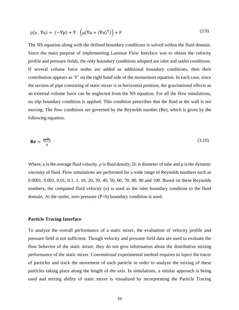
FIGURE 4.2 COMPARISON PLOT OF PRESSURE DROP (∆P) VS REYNOLDS NUMBER (RE) FOR ALL
STATIC MIXER GEOMETRIES FOR REYNOLDS NUMBER 0.0001 TO 100. .................................... 43
FIGURE 4.3 COMPARISON OF PRESSURE FIELD CONTOUR PLOTS (PA.S) FOR ALL STATIC MIXER
GEOMETRIES AT RE = 30. ........................................................................................................ 45
FIGURE 4.4 COMPARISON OF VELOCITY CONTOUR PLOTS (M/S) FOR ALL STATIC MIXER GEOMETRIES
AT RE = 30. ............................................................................................................................. 48
FIGURE 4.5 COMPARISON OF SHEAR RATE VS REYNOLDS NUMBER CONTOUR PLOTS FOR ALL STATIC
MIXER GEOMETRIES AT RE = 30. ............................................................................................. 51
FIGURE 4.6 COMPARISON PLOTS OF SHEAR RATE (Γ) VS REYNOLDS NUMBER FOR SMX,
PERFORATED SMX D/20 MAXIMUM NUMBER, SMX WITH CIRCULAR SERRATIONS, SMX WITH
TRIANGULAR SERRATIONS AND SMX WITH SQUARE SERRATIONS STATIC MIXERS. ................. 52
ix
FIGURE 4.7 COMPARISON OF EXTENSIONAL EFFICIENCY CONTOUR PLOTS FOR ALL STATIC MIXER
GEOMETRIES AT RE = 30. ........................................................................................................ 55
FIGURE 4.8 COMPARISON OF EXTENSIONAL EFFICIENCY VS REYNOLDS NUMBER (RE) CONTOUR
PLOTS FOR SMX, PERFORATED SMX D/20 MAXIMUM NUMBER, SMX WITH CIRCULAR
SERRATIONS, SMX WITH TRIANGULAR SERRATIONS AND SMX WITH SQUARE SERRATIONS
STATIC MIXERS. ...................................................................................................................... 56
FIGURE 4.9 SAME INITIAL POSITION OF BINARY COLOURED PARTICLE TRACER AT INLET FOR ALL
STATIC MIXER GEOMETRIES. ................................................................................................... 58
FIGURE 4.10 COMPARISON OF DISTRIBUTION OF BINARY COLOURED PARTICLE TRACER CONTOUR
PLOTS FOR ALL STATIC MIXER GEOMETRIES AT RE = 30. ......................................................... 60
FIGURE 4.11: COMPARISON OF STANDARD DEVIATION VS NUMBER OF MIXING ELEMENTS PLOT FOR
ALL THE STATIC MIXER GEOMETRIES AT RE = 30. ................................................................... 60
FIGURE 5.1 SMX STATIC MIXER GEOMETRY 8 ELEMENTS WITH ADDITIONAL PIPE INLET FOR THE
INITIATOR INFLOW .................................................................................................................. 71
FIGURE 5.2 CIRCULATED SMX SERRATED STATIC MIXER GEOMETRY 8 ELEMENTS WITH
ADDITIONAL PIPE INLET FOR THE INITIATOR FLOW .................................................................. 71
FIGURE 5.3 COMPARISON OF CONCENTRATION OF RESULTING POLYACRYLAMIDE FOR (A) SMX
GEOMETRY (B) CIRCULAR SERRATED SMX GEOMETRY .......................................................... 72
FIGURE 5.4 COMPARISON OF CONCENTRATION OF INITIATOR FOR (A) SMX GEOMETRY (B)
CIRCULAR SERRATED SMX GEOMETRY .................................................................................. 72
FIGURE 5.5 COMPARISON OF CONCENTRATION OF MONOMER FOR (A) SMX GEOMETRY (B)
CIRCULAR SERRATED SMX GEOMETRY .................................................................................. 73
FIGURE 5.6 VARIATION IN REACTION RATE ALONG THE LENGTH OF REACTOR FOR SMX GEOMETRY
............................................................................................................................................... 74
FIGURE 5.7 VARIATION IN REACTION RATE ALONG THE LENGTH OF REACTOR FOR CIRCULAR
SERRATED SMX GEOMETRY ................................................................................................... 74
FIGURE 5.8 VARIATION IN MONOMER CONVERSION ALONG THE LENGTH OF REACTOR FOR SMX
GEOMETRY FOR RE 30 ............................................................................................................ 76
FIGURE 5.9 VARIATION IN MONOMER CONVERSION ALONG THE LENGTH OF REACTOR FOR
CIRCULAR SERRATED SMX GEOMETRY FOR RE 30 ................................................................ 76

x
FIGURE 5.10 VARIATION IN MONOMER CONVERSION ALONG THE LENGTH OF REACTOR FOR BOTH
STATIC MIXER GEOMETRIES FOR RE 100 ................................................................................. 77
FIGURE 5.11 VARIATION IN MONOMER CONVERSION ALONG THE LENGTH OF REACTOR FOR BOTH
STATIC MIXER GEOMETRIES FOR RE 300 ................................................................................. 78

xi
List of Tables
TABLE 2.1 INDUSTRIAL APPLICATIONS OF STATIC MIXERS [12] ...................................................... 10
TABLE 2.2: COMMERCIALLY AVAILABLE STATIC MIXERS [12] ....................................................... 12
TABLE 3.1 DIMENSIONS OF ALL STATIC MIXER GEOMETRIES .......................................................... 29
TABLE 4.1 INLET CONDITIONS AND INPUT PARAMETERS USED FOR ALL STATIC MIXER GEOMETRIES
............................................................................................................................................... 39
TABLE 4.2 FINAL COMPARISON OF STATIC MIXERS ........................................................................ 62
TABLE 5.1 INITIAL CONDITION AND INPUT PARAMETERS FOR HOMOPOLYMERIZATION OF
ACRYLAMIDE .......................................................................................................................... 65
TABLE 5.2 COMPARISON OF PARAMETERS TO ANALYZE THE PERFORMANCE OF SMX AND
CIRCULAR SERRATED SMX FOR RE 30 ................................................................................... 79

xii
List of Abbreviations and Notations
SM ─ Static mixer
CFD ─ Computational Fluid Dynamics
ISG ─ Interfacial Surface Generator (ISG)
Komax CT mixer ─ Komax Custody Transfer mixer
LIF ─ Laser Induced Fluorescence
Re ─ Reynolds number
LB ─ Lattice Boltzmann
LDA ─ Laser Doppler Anemometry
CMC ─ Carboxy Methyl Cellulose
CAD ─ Computer Aided design
NS ─ Navier-Stokes equation
ODE ─ Ordinary Differential Equations
COV ─ Coefficient of Variation
CSTR ─ Continuous Stirred Tank Reactor
EOR ─ Enhanced Oil Recovery
PAM ─ Polyacrylamide
HPAM ─ Hydrolyzed Polyacrylamide
Nx ─ Number of cross-bars over the width of channel
Np ─ Number of parallel cross-bars per element
θ ─ Angle between opposite cross-bars
D ─ Diameter of mixer element
L ─ Length of the pipe
l ─ Length of mixer element
l/D ─ Length to Diameter ratio
Dt ─ Pipe Diameter
xiii
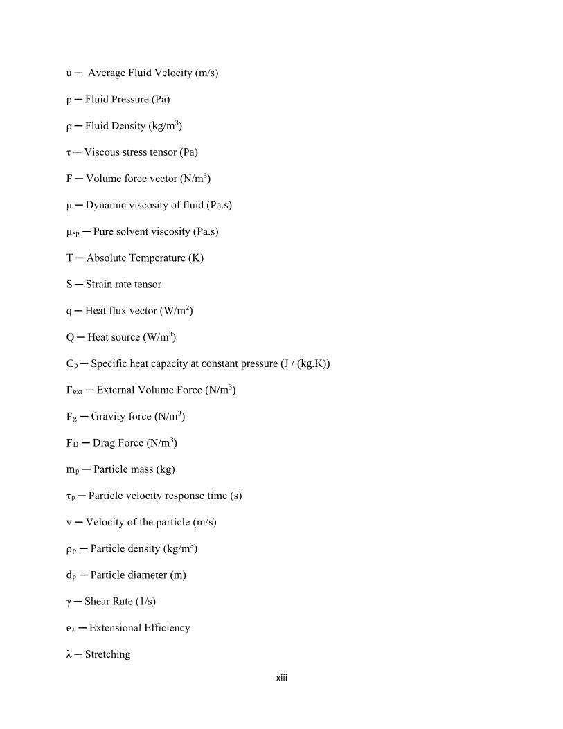
u ─ Average Fluid Velocity (m/s)
p ─ Fluid Pressure (Pa)
ρ ─ Fluid Density (kg/m3)
τ ─ Viscous stress tensor (Pa)
F ─ Volume force vector (N/m3)
μ ─ Dynamic viscosity of fluid (Pa.s)
μsp ─ Pure solvent viscosity (Pa.s)
T ─ Absolute Temperature (K)
S ─ Strain rate tensor
q ─ Heat flux vector (W/m2)
Q ─ Heat source (W/m3)
Cp ─ Specific heat capacity at constant pressure (J / (kg.K))
Fext ─ External Volume Force (N/m3)
Fg ─ Gravity force (N/m3)
FD ─ Drag Force (N/m3)
mp ─ Particle mass (kg)
τp ─ Particle velocity response time (s)
v ─ Velocity of the particle (m/s)
ρp ─ Particle density (kg/m3)
dp ─ Particle diameter (m)
γ ─ Shear Rate (1/s)
eλ ─ Extensional Efficiency
λ ─ Stretching

xiv
δ ─ Lyapunov exponent
∆ ─ Change
∇ ─ Divergence Operator
∆P ─ Pressure Drop (Pa)
Z ─ Pressure Drop Ratio
f ─ Friction Factor
∆PSM ─ Pressure drop across static mixer (Pa)
∆PET ─ Pressure drop across empty tube (Pa)
Fs ─ Shear Force (N)
As ─ Area of shearing plane (m2)
εv ─ Viscous shear stress (N/m2)
V – Volume (m3)
ω ─ Vorticity tensor
Ni ─ Number of particles falling in ith grid cell
N� ─ Average number of particles in each grid cell
n ─ Number of cells in grid
σN ─ Number based standard deviation
k – Reaction rate constant
k’ ─ Huggins constant
c ─ Concentration of species
D ─ Diffusion coefficient (m2/s)
R ─ Reaction rate expression for the species ((mol) / (m3.s))

1
CHAPTER 1: Introduction
1.1 Static Mixers
Mixing is one of the important phenomena which is essential in both unit operations and unit
processes. Mixing is a process in which two or more components are physically brought into
contact with each other in order to create a homogenous system. Depending on the process
requirements, mixing operation can be either a single phase or multiphase system. Further, the
components involved in mixing operation (e.g. solids, liquids and gas), can be either miscible or
immiscible into each other. In applications, where a completely mixed homogeneous system is
required to obtain the desired product, mixing plays an important role in terms of the quality of the
final product quality, energy costs and turnover of the process.
Mixing can be achieved in two ways: one with agitator and other one without an agitator. The first
approach involves the use of conventional mixers while the second approach involves the use of
static mixers. Conventional mixers include rotators, impellers, stirrers and agitators. Since these
mixers have moving parts, they are also called as dynamic mixers. Dynamic mixers are powered
by electric motors. Dynamic mixers convert the electrical energy of motor into rotary mechanical
energy. Flow regime is one of the important factors in the selection of mixing devices. Dynamic
mixing is often applied when the flow is in turbulent region. In laminar flow region and for highly
viscous fluids, dynamic mixers require huge amount of power to mix the fluid; which makes them
an expensive choice compared to motionless mixers. For highly viscous fluids in the laminar
region, static mixers (SMs) require relatively less power and they perform better than the
conventional agitator mixers in terms of mixing operation. Since SMs have no moving parts, they
are easy to maintain and are often known as motionless mixers. SMs use the pressure difference
or kinetic and potential energy of the fluid, for the flow to occur. The momentum of the flowing
fluid is used to create velocity gradients. Random or structured flow patterns of the fluid are
generated by SMs, which involves splitting, shearing, rotating, twisting, accelerating, decelerating
and recombining of fluid streams [1].

2
Depending on the process requirements, SMs can be used for continuous operation. SMs can be
used for applications involving both Newtonian and non-Newtonian fluids. When it comes to
installation of mixing device in very small space, SMs are often preferred to conventional mixers.
Other benefits of using SMs to that of dynamic mixers are low equipment cost, low operation cost,
less scaling and erosion, narrow residence time distribution, near plug flow behavior and high
radial mixing [2].
1.2 Research Objective
The main objective of this research work is to investigate the effects of design modifications in
existing SM geometries to achieve improved mixing and minimize the pressure drop. There are
several standard SM geometries available in the industry (like Koch-Sulzer SMX and Chemineer
Kenics static mixer), which are being utilized in various industrial operations. By increasing the
number of mixing elements it is always possible to obtain an improved axial dispersion but at the
cost of very high pressure drop. Therefore, our research objective is to use perforations in the
mixing elements. Further, introduction of different types of serrations such as triangular, square
or half-circular shapes along the edges of each blade is proposed to serve as an alternative
modifications to the perforations. By incorporating different shapes of serrations in a static mixer
geometry, improved dispersion and distributive mixing can be achieved. An additional benefit of
the proposed modifications would be minimizing the pressure drop, which in turn minimizes the
energy cost.
The main focus is to propose a modified SM geometry with precise dimension, so that it can be
used in applications where enhanced mixing is achieved. In the current study, computational
investigation is carried out to analyze the mixing performance of static mixers. Computational
Fluid Dynamics (CFD) simulations are performed using COMSOL Multiphysics software for
perforated SMX and serrated SMX geometries. The results of CFD simulations are compared with
SMX geometry to study their mixing performance. The effect of the number of perforations and
the size of perforations has been studied to obtain better mixing with minimum pressure drop. In
the case of serrated SM geometries, the simulations are performed and analyzed to estimate the
best serration pattern for efficient mixing.

3
1.3 Thesis Outline
This thesis is organized in the following structure. Chapter 2 explains different types of static
mixers and their applications in various industries. It also includes the previous studies performed
on different static mixers using CFD approach. In Chapter 3, the methodology to carry out the
CFD simulations in COMSOL is discussed. Different physic models and related numerical
equations used in the CFD simulations are explained in detail. Brief description about the meshing
of geometry and solvers of COMSOL to solve different sets of equations are presented. In Chapter
4, the results from CFD simulations performed on different static mixers are analyzed and the
performance is compared in terms of different parameters. Based on the results of these parameters,
dispersive and distributive mixing capacity of static mixers have been analyzed. In Chapter 5,
computational modeling for very highly viscous non-Newtonian fluidic system is presented.
Synthesis of homopolymer system using a modified SM geometry is discussed in this chapter.
Finally, the conclusions and recommendations for future work are presented in the last chapter.
4
CHAPTER 2: LITERATURE REVIEW
This chapter is divided into three parts. The first part discusses about different types of static
mixers based on their geometry. In the second part, industrial applications of static mixers have
been illustrated in the form of tables and charts. In the last part, application of CFD for helical,
non-helical and new type of static mixer geometries are discussed.
2.1 Classification of Static Mixers
Static mixers or motionless mixers are basically used for mixing or blending fluids of different
densities and viscosities. They are widely used in process industry for continuous operations. In
any continuous operation involving SM, external pumps are used for the fluid to flow across the
static mixer elements. Since static mixers have no moving parts, mixing solely depends on the
movement of fluid streams which eventually gets twisted, rotated, spread and recombined by the
internal geometry of SM. Due to this, momentum of fluid is converted into mechanical energy of
static mixing at the expense of pressure drop. Energy supplied by the external pumps is lost in
terms of pressure drop, which is a major consequence of static mixing. From engineering
perspective, an ideal static mixer would be the one which delivers desired mixing with a minimum
pressure drop. Each static mixer has a unique geometry and is designed for a particular range of
operations. Each one performs quite differently from others with respect to the flow behavior
which in turn affects the mixing of fluids.
From the reported literature and publications, static mixers can be classified into five main
categories:
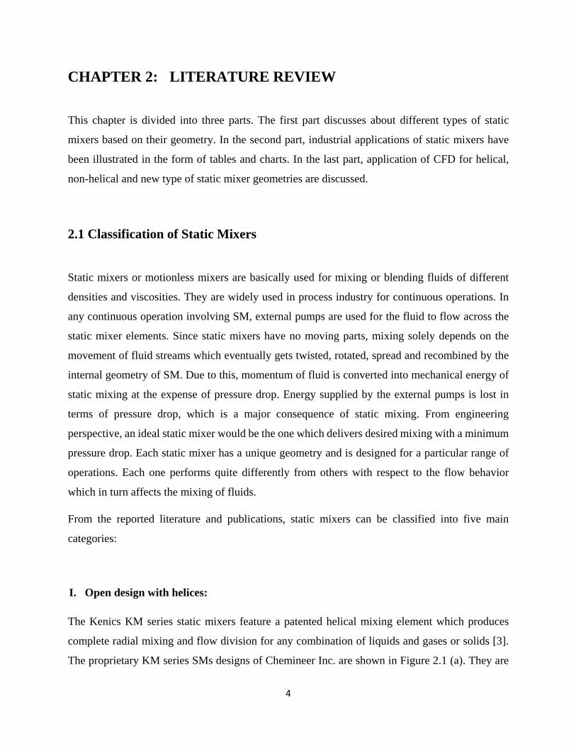
I. Open design with helices:
The Kenics KM series static mixers feature a patented helical mixing element which produces
complete radial mixing and flow division for any combination of liquids and gases or solids [3].
The proprietary KM series SMs designs of Chemineer Inc. are shown in Figure 2.1 (a). They are

5
used for laminar flow, transitional flow and turbulent flow applications. These type of SMs are
distinguished based on the method of manufacturing only. KMS and KME type mixers are fixed
to the inner wall of housing, whereas KMR mixer can be easily detached from the housing. KMA
mixer can be installed in any existing housing. Figure 2.1 (b) shows ERESTAT mixer [4], which
consists of an alternate left handed or right handed baffles. Due to this type of structure, there are
various channels through which single fluid stream splits and flows. Further, an N-shaped static
mixer [5] with twisted mixing elements is also shown in the same figure. This type of static mixer
creates variable channel cross sectional areas. Another static mixer which comes under the same
category is Hi-mixer element [6]. It has a solid cylinder and on both ends of cylinder two parallel
holes are countersunk. In each hole, a helix element with a twist of 180° is fitted.
II. Open design with blades:
Mixing in SMs is achieved by splitting and diverting the input fluid streams. Major advantage of
SMs with open blade design is that, in the turbulent flow applications they enhance the random
dispersion of sub-streams. ‘Charles Ross and Son’ has developed LPD and LLPD static mixers
based on this kind of design (shown in Figure 2.1 (c)). Chemineer has developed its own open
blade design motionless mixer. It is known as HEV high-efficiency static mixer (shown in Figure
2.1 (d)). It can handle all type of turbulent-flow mixing applications regardless of line size or shape.
KOMAX SYSTEM Inc. has designed a unique open blade mixer which is known as KOMAX
Custody Transfer meter. It is shown in the Figure 2.1 (e). The Komax CT (Custody Transfer) mixer
was specially designed to solve conventional custody transfer mixing problems in crude oil
industry. Lightnin Inc. has developed the most cost effective open blade design of static mixer,
which is known as ‘series 45’ (Figure 2.1 (f)). It features specific pattern of splitting, rotating and
mixing of the fluid streams in laminar, transitional and turbulent flow regimes.
6
(c)
(e)
(g)
(i)
(YXZET, Dr. KARG GmbH,Affalterbach)
(BRAN and LOBBE, Norderstadt)
(TORAY, Tokyo)
(b)
(d)
(f)
(h)
(j)
(a)
7
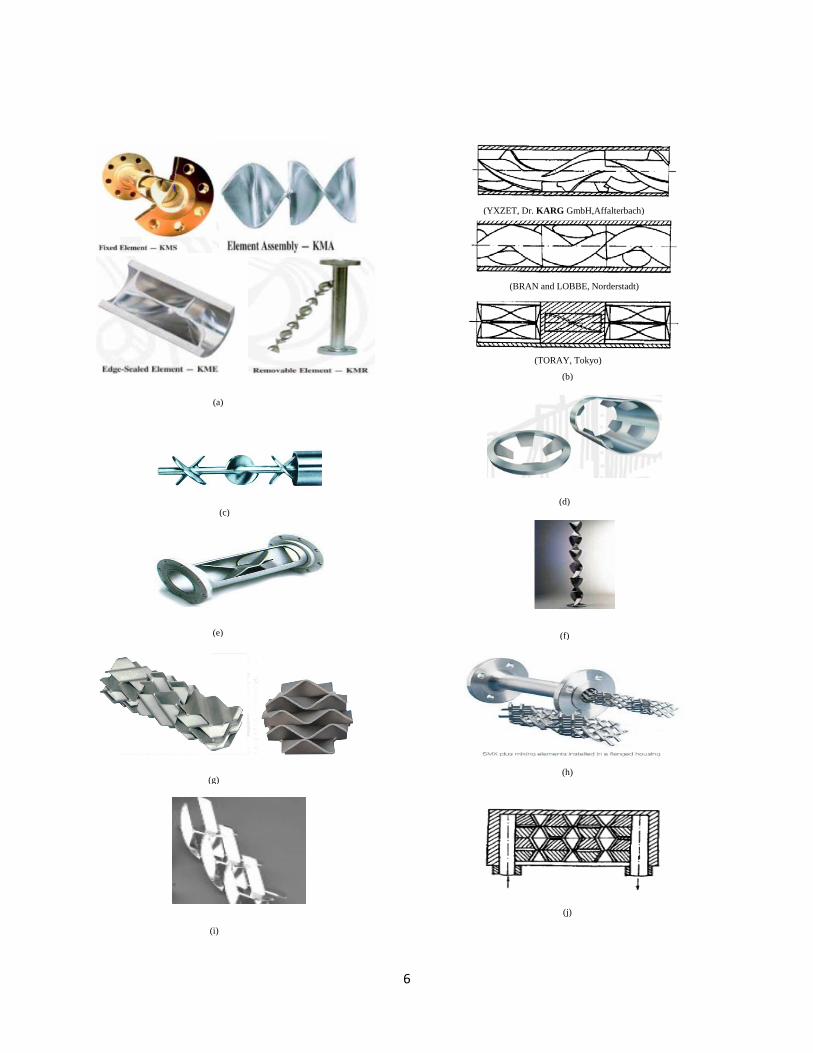
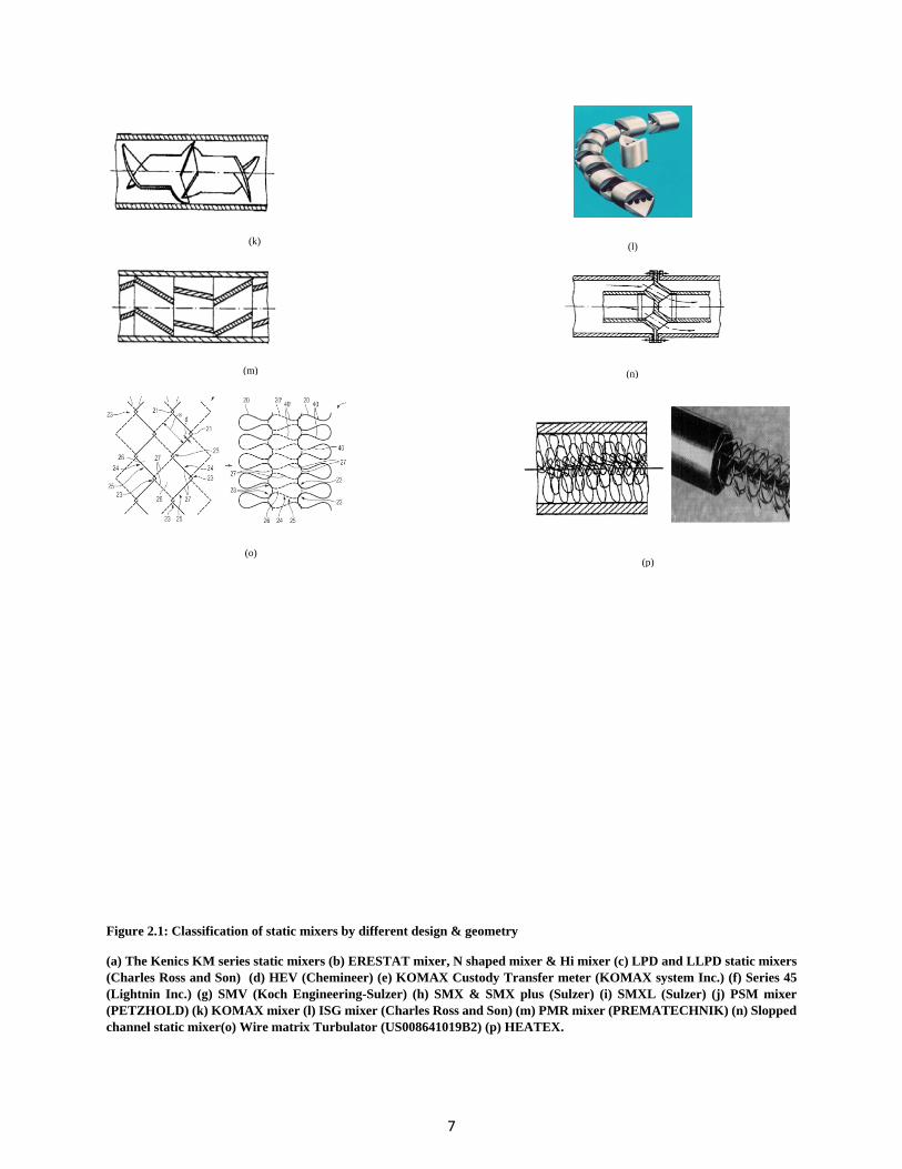
Figure 2.1: Classification of static mixers by different design & geometry
(a) The Kenics KM series static mixers (b) ERESTAT mixer, N shaped mixer & Hi mixer (c) LPD and LLPD static mixers (Charles Ross and Son) (d) HEV (Chemineer) (e) KOMAX Custody Transfer meter (KOMAX system Inc.) (f) Series 45 (Lightnin Inc.) (g) SMV (Koch Engineering-Sulzer) (h) SMX & SMX plus (Sulzer) (i) SMXL (Sulzer) (j) PSM mixer (PETZHOLD) (k) KOMAX mixer (l) ISG mixer (Charles Ross and Son) (m) PMR mixer (PREMATECHNIK) (n) Slopped channel static mixer(o) Wire matrix Turbulator (US008641019B2) (p) HEATEX.
(k)
(m)
(o)
(l)
(n)
(p)

8
III. Corrugated-plates :
To intensify mass transfer between immiscible fluids, Koch Engineering-Sulzer has developed
SMV mixer which is shown in Figure 2.1 (g). It is used in turbulent and transitional flow regime.
SMV mixer is made of corrugated plates that form open, intersecting channels in which the flow
is divided into many sub-streams. It is a high performance inline static mixer capable of mixing
low viscosity liquids, blending gases, dispersing immiscible liquids and creating gas-liquid
dispersions with a very high degree of mixing in a short length.
IV. Multi-layers design:
Instead of having a series of end to end components, multi-layer design elements repeatedly divide
the fluid stream into different layers and spread them over the entire cross-section of the pipe. A
major benefit of this kind of design is that, it can mix extremely high viscosity and/or very high
volumetric ratio of fluids. Sulzer has developed and patented SMX and SMX plus mixers based
on this design (shown in Figure 2.1 (h)). Mixing is accomplished in a short length with a very high
degree of mixing. However for long pipe sections, where continuous mixing action with low
pressure drop is required, SMXL mixer is used (shown in Figure 2.1 (i)). Further PSM mixer [7]
(shown in Figure 2.1 (j)) falls under the same category, which is constructed from individual plates.
These plates have central holes, conical & rectangular slots. Due to this type of structure, fluid
passing through the conical space is subdivided by tangentially arranged slots. The fluid
subsequently flows further through slots and openings. Another multi layered static mixer known
as KOMAX [8] is constructed from slotted sheet metal pieces with bent ends. The KOMAX mixers
(shown in Figure 2.1 (k)) uses triangular shaped channels for the fluid flow.
V. Closed design with channels or holes :
Closed designs are typically required for blending of minor components of a viscous stream.
Charles Ross and Son has developed Interfacial Surface Generator (ISG) mixer (shown in Figure
2.1 (l)). ISG mixers are capable of mixing the fluid streams having extremely high viscosity ratio
of 250000:1 or more than that. Highly viscous fluid streams are repeatedly combined and
subdivided into layers until a homogeneous mixture is achieved. The Ross ISG mixer is ideal for
applications where mixing elements must be removed for fast and easy cleaning. The PMR mixer
[9] (shown in Figure 2.1 (m)) is also a closed design static mixer, typically consisting of partial
9
tube sections arranged obliquely. Fluid stream is twisted and directed by the partial tubes and the
spaces among them. Static mixer shown in the Figure 2.1 (n) can be used to invert the fluid streams
of different velocities. It has two guiding pipes mounted in the direction of flow. The fluid stream
which flows through the central section has a high mean velocity. Cross channels divert this fluid
stream towards the pipe wall where fluid velocities are very low. These cross channels also divert
the fluid streams which are flowing adjacent to the wall towards the central zone of pipe. This
static device can be used to achieve uniform residence time distribution of the fluid.
VI. Wire matrix Turbulators :
Figure 2.1 (o) shows a wire framed static mixer. These kind of static mixers possess loops, which
are formed substantially by wire knitting. Wire structure is framed by interlacing one or more wires
to form the loops. It gives very high stability to the wire mesh structure. Wire structured static
mixer is used in the diversion station of a steam turbine plant [10]. This type of static mixer in
conjunction with a diversion station enables the effective cooling of water vapor by mixing it with
water. Significant advantage of wire structure of static mixer is vortex generation, which causes
transverse mixing of water vapor with water drops. Further, water drops are separated on a wire
mesh. Quick evaporation of water and hence more cooling can be achieved by incorporating this
type of static mixers. Another wire framed static mixer is “HEATEX” (shown in Figure 2.1 (p))
[11]. In this type of SM, a series of wire loops are wound on a central wire core. Each wire loop is
inclined at a certain angle with respect to the central wire core. A higher loop density gives more
tube wall contact per unit length. Depending on the required degree of mixing, loop density of
HEATEX is selected.

10
2.2 Applications of Static Mixers:
Table 2.1 Industrial applications of static mixers [12]
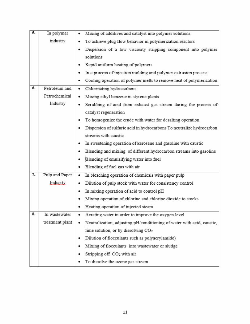
11

12
Table 2.2: Commercially available static mixers [12]

13
Figure 2.2 Chart of applications of static mixers [13],[14]
14
2.3 Application of Computational Fluid Dynamics (CFD)
Experimental investigation of performance of different SMs is expensive and time consuming task.
Till late 1970s several experimental studies have been conducted to understand the flow behavior
and mixing performance of the static mixers. However, with the development of CFD and faster
computers, it has become much easier to analyze the mixing characteristics of static mixers for
various types of fluids. Since then, several simulations were performed to understand thoroughly
the mixing performance of different SMs. With the help of computational techniques, tedious
information such as determination of flow path of fluid in static mixers, information on velocity
profiles, temperature profiles and pressure field can be obtained. CFD simulations give qualitative
and quantitative information related to mixing performance by studying particle trajectories,
residence time distribution or by analyzing concentrations if reaction kinetics is involved. Based
on the results of CFD simulations and numerical models, correlations for mixing parameters can
be developed which are helpful for designing and optimization of static mixers [15].
2.3.1 Helical static mixers
Several attempts have been made using CFD modeling in early 1980s to develop models for
analyzing the flow in SMs. For the flow of Newtonian fluid in three dimensional geometry, Roache
[16] proposed a numerical scheme to solve the flow equations in terms of velocity and pressure.
In 1983, Shintre and Ulbrecht [17] developed a flow model for the dispersive and distributive
mixing of Newtonian fluids within two sheets of Koch-Sulzer mixer. This model is extended
further for non-Newtonian fluid too. The first publication involving CFD simulations for the study
of mixing properties of Kenics mixer is dated in 1985 [18]. In this study, CFD simulations are used
to mix two similar fluids. The final flow visualization results are in good agreement with the
published experimental results, which makes it a reliable computational tool for other modified
SM geometries.
There are several research groups, which worked on the helical static mixers to get the pressure
drop and the mixing characteristics. For that purpose different criteria and parameters have been
used to define an extent of mixing in the static mixers. To a certain extent their research is based
15
on the work published by Ottino [19]. Earlier Dackson and Nauman [20] , Ling and Zhang[21]
carried out computational studies for the fluid flow in static mixer. However to achieve the solution
for flow field, they ignored the transition of flow between the mixer elements in their studies. This
factor has been taken into consideration by Hobbs and Muzzio [22]. They used finite element
software FLUENT to numerically characterize the low Reynolds number flow in Kenics mixer.
They also used particle tracer to investigate the extent of mixing computationally. Similar studies
have been conducted by André Bakker et al [23] to gain insight in the mixing mechanism of two
chemical species in inline Kenics static mixers. Based on the work presented by Hobbs and Muzzio
[24], further studies were performed by Fourcade [25]. They used finite element code POLY3D to
characterize the mixing characteristics of SMs and validated it with the results of laser induced
fluorescence (LIF).
Interestingly, these studies were focused on low Reynolds number (Re) Newtonian fluid only. In
1998, O. Byrde et al [26] published a work for non-creeping flow conditions (Re=100) to
determine the optimal twist angle of Kenics static mixer. So far, very limited knowledge is
available in the literature for higher Reynolds number (Re=100 to Re=1000). Validation of CFD
results with the literature data is important for relatively higher Reynolds number (Re > 200) and
for coarse meshing. W. F. C. van Wageningen et al [27] has undertaken the dynamic flow study in
Kenics mixer for Reynolds number varying from 100 to 1000. They used two different numerical
methods namely Lattice Boltzmann (LB) and FLUENT. They validated flow field and dynamic
behavior of fluid to the results of laser Doppler anemometry (LDA) experiments. Ramin Rehmani
et al [28] performed detailed study on Kenics mixer for Laminar flow and Turbulent flow region.
They used second order numerical method (FLUENT) and validated the CFD model with the
literature data. Furthermore, they extended their study to non-Newtonian pseudo plastic fluids.
Recently, a CFD model of Kenics mixer consisting of 10 elements is published which focuses on
the usage of SM in water treatment plant [29]. This study involved calculations of the flow field
and mixing characteristics for turbulent flow region (Reynolds number 103 to 106). Another
publication, which involved the use of Kenics static mixers, has demonstrated the application of
CFD simulation for non-Newtonian fluids. In this study, sodium carboxy methyl cellulose (CMC)
is used as a non-Newtonian fluid and numerical simulations are performed for cross model and

16
non-Newtonian power law model [30]. Apart from getting information about flow behavior, heat
transfer process in SMs is also studied using CFD simulations. Recently, some studies have been
undertaken to know the thermal efficiency of static mixers using CFD simulations [31]. Maciej
konopacki [32] published their work on how to calculate numerically the flow and temperature
distribution in SMs using CFD.
2.3.2 Study of non-helical static mixers As yet, the studies indicated above discuss about the application of CFD simulations for the helical
type of static mixers. Due to comparatively simple geometry and ease of meshing in the CFD
software, helical element SMs are more convenient choice over SMX geometry. In late 90s, several
research groups worked on non-helical static mixers (mostly SMX mixer) to numerically
investigate the mixing performance of SMs. Among all, two research groups namely: Tanguy et
al and Rauline et al have major contribution towards investigating the mixing performance of SMX
mixers using CFD simulations [33].
Based on the literature review, it is observed that first non-helical SM study using CFD was
reported in 1990. Tanguy et al [34] studied three-dimensional modelling of the flow through a
LPD Dow-Ross static mixer. In their study two mixing elements over a wide range of flowrates
were used and the obtained results were validated on the basis of pressure drop. Mickaily-Huber
et al. [35], reported a work on numerical simulations of mixing and flow characteristics induced
by Sulzer SMRX, which is a simplified version of the proprietary SMR mixer. SMX is one of the
most commonly used non-helical static mixers. Due to its complex geometry, experimental
investigation does not provide as precise and versatile means of local measurements as those in
the case of CFD software. Louis Fradette et al [36], used POLY3D simulation package to obtain
pressure drop and velocity field information of fluid flowing in SMX mixer.
Most of the research groups mainly worked towards validating flow behavior of fluid in terms of
pressure and velocity variations. Rauline et al [33], used five criteria which are namely extensional
efficiency, stretching, mean shear rate, intensity of segregation and pressure drop. They performed
numerical simulations using POLY3D for six different static mixers (Kenics, Inliner, LPD,

17
Cleveland, SMX and ISG) in laminar regime. Numerical results obtained for each type of static
mixer was in good agreement with the literature values. Considering the fact that some variables
like flow rate, mixer diameter and number of mixing elements were not taken into considerations,
Rauline et al extended their work further to take into account these variables in numerical
simulations. The performance of Kenics and SMX were assessed based on mean shear rate, mixer
length, Lyapunov exponent and intensity of segregation [37]. They established empirical pressure
drop and mixer length relations for these mixers and concluded that SMX mixer is more efficient
than Kenics mixer if very limited space is available for mixing of fluids.
O. Wuensch, G. Boehme [38] illustrated how to numerically simulate single phase highly viscous
fluid by combination of Eulerian and Lagrangean method using SMX mixer. The advantage of
hybrid method is that it can be applied to other geometries as well. In general, particle tracer is
used in almost all CFD softwares to estimate the mixing parameters like intensity of segregation.
This study explains how to calculate velocity fields numerically and track the particle motion
dynamically using Eulerian and Lagrangean approaches for low Reynolds number creeping flow.
With the help of CFD simulations, mixing of liquids at the microscale can also be analyzed. The
mixing efficiency of static micromixers made of intersecting channels and helical elements have
been estimated using FLUENT-5 CFD program [39]. However, all these earlier mentioned studies
of SMX simulations did not account the effects of increased flow rate and inertia. J. M. Zalc et al
[40] studied the flow and mixing characteristics of SMX mixer at low and moderate Reynolds
number by means of CFD simulations. They demonstrated direct comparison of computed mixing
rates to experimentally measured values. Exponential decrease in coefficient of variation with
increasing axial distance was evident from the CFD simulations results. Recently, the effects of
non-Newtonian shear thinning fluid on pressure drop and mixing in the case of SMX have been
examined by Shiping Liu using CFD modeling [41]. The pressure drop ratio and friction factor
were analyzed with varying power-law index.

18
2.3.3 Study of modified or new type of static mixers
As mentioned in the previous sections, several research groups have performed and reported the
numerical comparison of SMX and helical Kenics static mixers. Although these research groups
used different CFD softwares, almost same parameters have been used to compare the performance
of these two static mixers. The common conclusion they proposed is that SMX mixer manifests
higher fluid mixing performance than Kenics but at the cost of higher pressure drop [42]. Based
on this fact, researchers focused more on improvement or design modifications in SMX
geometries.
Shiping Liu et al [43] investigated the characteristics of the flow field in a standard SMX static
mixer by CFD simulations. Further, the effects of crossbar number or equivalent bar width of
mixer element was studied in terms of mixing and pressure drop. As a design modification to the
standard SMX design, the aspect ratio of one single element of SMX mixer was changed. The
proposed new designs of static mixers had an aspect ratio of 2/3 and 1/2. The new static mixer
element with denser arrangement of crossbars and smaller aspect ratio showed higher mixing rate
and strain rate distribution than SMX mixer.
Static mixers are always used to homogenize viscous liquids at the cost of high pressure drop. For
this purpose, significant efforts have been put in by various research groups to improve mixing
and at the same time minimize the pressure drop by introducing new static mixer geometries. J.C.
van der Hoeven et al [44], used newly designed multi-flux static mixer in which fluid is
successively stretched, cut and stacked. In the channel of this device, several ‘mixing elements’
are present. They used 3D numerical simulations to investigate the causes of inhomogeneity of
fluid in standard design. It was proposed that by introducing additional elements with separating
walls at the inlets and at the outlets of the mixing elements, tremendous increase in the
homogeneity can be achieved. These changes in arrangements of elements and their effects were
verified by simulations and experiments.
In 2008, Mrityunjay K. Singh et al [45] developed new type of static mixers by changing the
number of cross-bars in standard SMX mixer. Quantitative mixing analyses based on the mapping

19
method is performed to understand the stretching of the fluid within the SMX geometry. Based on
the concept of three design parameters namely: number of cross-bars over the width of channel
(Nx), the number of parallel cross-bars per element (Np), and the angle between opposite cross-
bars θ, several new static mixer geometries have been studied. These modified static mixers have
been referred as SMX (h) and SMX (n). It was observed that increasing Nx results into under-
stretching, whereas by decreasing Nx over-stretching occurs. Further, it was observed that because
of co-operating vortices, interfacial stretching becomes more effective with the increase in Np.
Based on the mapping method analyses, it was concluded that optimal stressing is achieved in
SMX(n) type of mixers which follows the design rule of Np = (2/3) Nx-1, for Nx = 3, 6, 9,12…
A new static mixer Cross-over-Disc has been studied to strip off the boundary layer and to make
strong radial mixing [46]. This new type of static mixer strips off the boundary layer entirely and
induces radial mixing. To analyze the mixing performance of Cross-over Disc SM, experimental
investigation is performed for highly viscous fluid (range from 190-250 Pa.s) using 14 elements.
Furthermore, a combination of this new SM with Sulzer SMX has been studied which decreases
the inhomogeneity to 2.1%-3.1% with a reasonable pressure drop. Due to special design of cross-
over-disc SM, it gave better performance than traditional static mixers.
2.4 Conclusion
Industrial applications of SMs have undergone a step-by-step growth with the development of
technology and computational techniques. Based on the work reported by several researchers, it
can be concluded that SMX gives better mixing but at the same time, it imposes higher pressure
drop than Kenics. Several research groups have worked towards the design modifications and new
static mixer geometry. These new designs of static mixers are promising in terms of mixing
performance. Since current research is focused about studying different SM geometries in terms
of flow and mixing behavior, computational studies carried out by several research groups would
be helpful in comparing the simulation results.

20
CHAPTER 3: Modeling and Methodology
3.1 Introduction
Setting up a computational model and carrying out simulations for fluid flow system is a faster
and more efficient method to study and improve the mixing behavior of static mixers. Most vital
part of any computational model is the accuracy of final simulation results. Higher the
requirements to achieve precise simulation results, more complicated the computational model
would be. Since complicated models are often computationally demanding and take longer time
to be solved, it is recommended to set up simplified model at the beginning of project. Depending
on the process requirements, complexities can be introduced gradually. The benefit of adopting
this type of multi-stage modeling strategy is that the effect of each refinement/complexity can be
fully apprehended before moving to the next stage. These complexities can be introduced in
different forms to any computational model. They can be introduced in terms of more complicated
geometry, or using more number of boundary conditions and/or physical properties, or using
multiple physic interfaces in computational model.
There are several commercial software products available that can be used to perform CFD
simulations. Each software has a different set of working environment and user interface.
However, the basic governing equations of each physics interface would be same. Fundamental
knowledge about physics to be used is necessary to create a computational model so that it would
represent a real experimental setup as closely as possible. In this research work, COMSOL
Multiphysics 5.0 is used to perform three dimensional CFD simulations of steady laminar flows
of incompressible Newtonian fluid in the various static mixers. Since COMSOL provides user-
friendly interface, computational model can be easily coupled to multiphysics problem and can be
solved simultaneously. COMSOL provides a robust platform, where various three dimensional
geometries can be either created within the software or imported from an external CAD software.
Different physics interfaces are used to solve various types of linear, non-linear, stationary and
time dependent problems. COMSOL works on finite element method to solve any computational
model.

21
To work with any CFD software, first it is important to understand the basic methodology of
building up a computational model. General procedure to set up a model in COMSOL begins with
creating or importing a geometry. Once the geometry is available in the COMSOL environment,
next step is to set up different physics interfaces. In the current work, Laminar Flow and Particle
Tracing interfaces are used to perform static mixer simulations, which is followed by meshing of
geometry. Meshing is important step for solving the model, since the accuracy of results depends
on selection of mesh size and the type of mesh. Once the mesh is selected, model is all set to be
solved using different solvers in COMSOL.
3.2 Geometry of Static Mixer
Computer Aided Design (CAD) is used for electronic drafting which makes use of computer
system for creation, modification, analysis and optimization of geometry [47]. Each CAD program
has a geometry kernel which depicts the object mathematically and calculates the results of
modeling operations. Since COMSOL Multiphysics has its own geometry kernel, various designs
can be created using geometry primitives and operations within the COMSOL environment. The
CAD tool in COMSOL also allows user to import and/or export the geometry from external
software to COMSOL environment which makes modeling easier for complicated 3D geometry.
To start the modeling, use of highly complicated geometry is not preferred initially. When it is
possible, the use of symmetric geometry or 2D cross-section of geometry is preferred to estimate
the results of modeling. In this research, 3D geometry of SMX static mixer and modified SMX
geometries are used as continuous mixer designs. In any computational modeling, geometry part
is more sensitive than others since it provides the information about the nature of flow and also
the information about the velocity and pressure variations occurring in different parts of the
geometry. All static mixers geometries are first designed in Autodesk AutoCAD software and
imported to COMSOL. Figure 3.1 shows the design of standard SMX static mixer used in the CFD
model. Each element of these static mixers are made of stacked lamella, which creates an intricate
network of flow channels. Each mixer element is placed at 90° rotation angle with respect to the
neighbouring element. All the elements are arranged axially along the length of the pipe. The
rotational arrangement impose maximum shear on the flowing fluid and the series of crossed
blades split the fluid stream repeatedly into layers spreading it all over the pipe cross section.

22
Figure 3.1 SMX static mixer geometry
Each mixer element has a diameter (D) of 0.0526 m and a length to diameter (l/D) ratio equal to
one. The thickness of each blade is 0.001 m. In all practical applications, static mixer assembly
has to slide inside the tube, the pipe diameter has to be kept 2-3% more than the diameter of the
static mixer element. In this case, the pipe diameter (Dt) is 0.053 m. Koch-Sulzer SMX static
mixer is the basic element for all the modifications carried out in this study. Different modified
SMX geometries used for computational modeling in this research work are shown in Figure 3.2
to Figure 3.9.
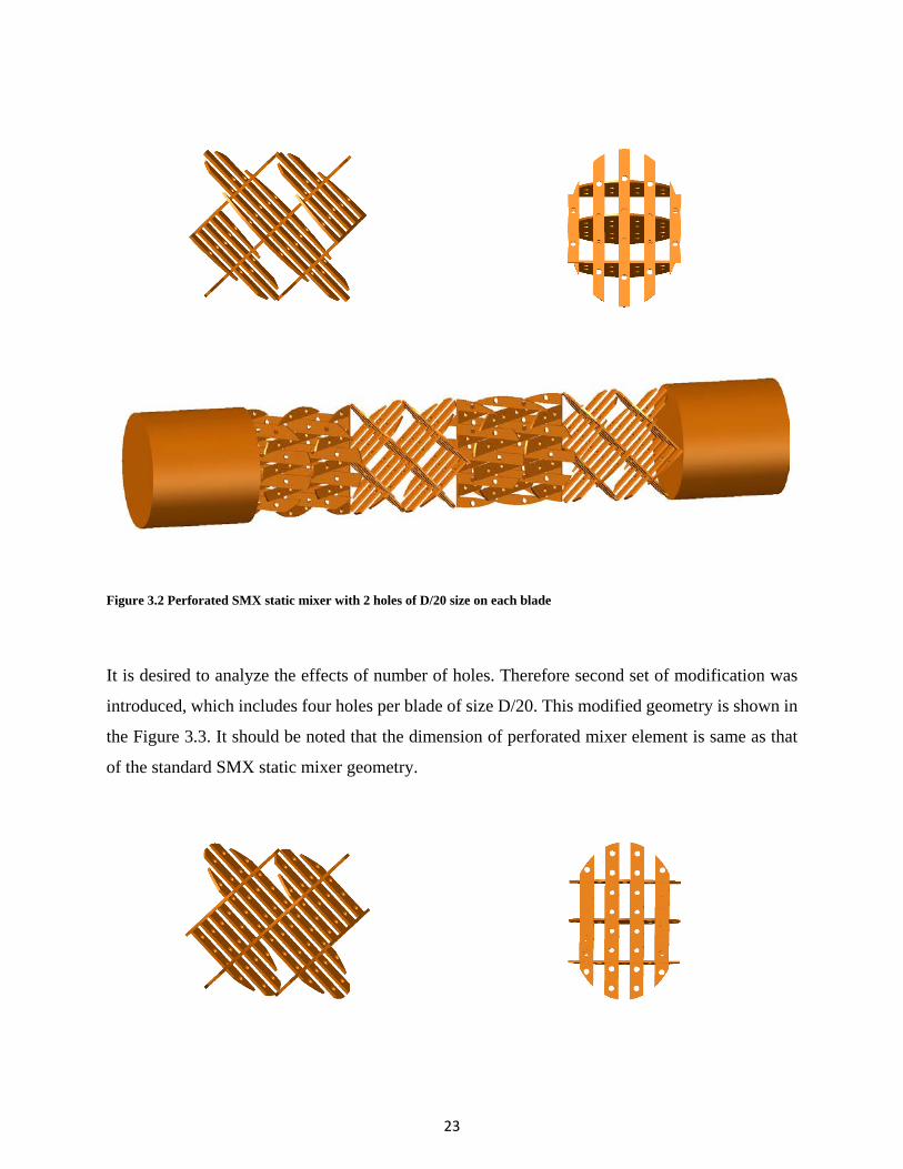
The first set of modifications had perforations of different sizes introduced on the blades of a
standard SMX geometry. Initially, two holes of size D/20 were introduced on each blade, which
is shown in Figure 3.2.
23
Figure 3.2 Perforated SMX static mixer with 2 holes of D/20 size on each blade
It is desired to analyze the effects of number of holes. Therefore second set of modification was
introduced, which includes four holes per blade of size D/20. This modified geometry is shown in
the Figure 3.3. It should be noted that the dimension of perforated mixer element is same as that
of the standard SMX static mixer geometry.
24
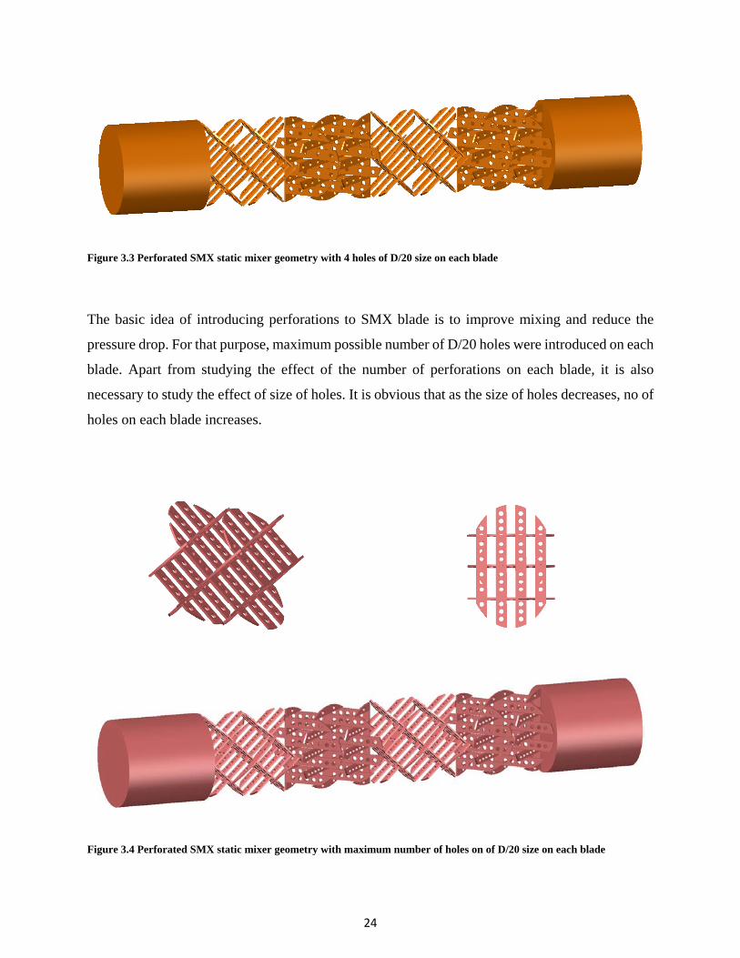
Figure 3.3 Perforated SMX static mixer geometry with 4 holes of D/20 size on each blade
The basic idea of introducing perforations to SMX blade is to improve mixing and reduce the
pressure drop. For that purpose, maximum possible number of D/20 holes were introduced on each
blade. Apart from studying the effect of the number of perforations on each blade, it is also
necessary to study the effect of size of holes. It is obvious that as the size of holes decreases, no of
holes on each blade increases.
Figure 3.4 Perforated SMX static mixer geometry with maximum number of holes on of D/20 size on each blade

25
Next modification is done by introducing the maximum number of perforations of size D/30 and
D/40 on each blade of the static mixer. Figure 3.5 shows perforated SMX geometry for maximum
number of holes of size D/30.
Figure 3.5 Perforated SMX static mixer geometry with maximum number of holes on of D/30 size on each blade
Figure 3.6 shows the modifications done in perforated SMX geometry for maximum number of
holes of size D/40. The fundamental approach to accommodate maximum number of holes is, the
distance between two consecutive holes should be marginally greater than the diameter of holes.
Based on this fundamental approach, maximum number of holes of size D/20, D/30 and D/40 were
accumulated on each blade. To select the best pattern of perforations, simulation results of all of
these modified SMX geometries were compared to the standard SMX geometry.

26
Figure 3.6 Perforated SMX static mixer geometry with maximum number of holes of D/40 size on each blade
The next set of modifications is done by introducing serrations on each blade of SMX element,
which is shown in Figure 3.7 to Figure 3.9. Circular, triangular and square pattern of serrations
were introduced on each blade of the mixer element. These type of serrations increases the
interfacial area on each blade, which in turn results in elongational flows. An additional benefit of
these serrations would be significant decrease in the pressure drop.
27
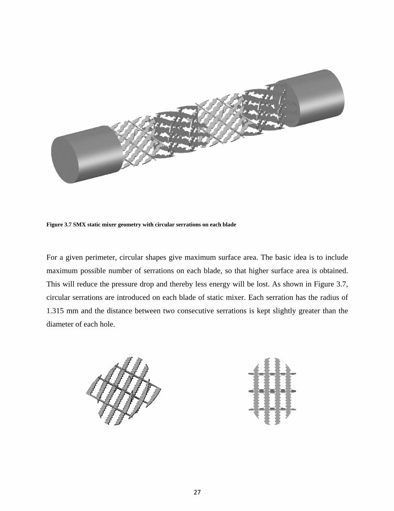
Figure 3.7 SMX static mixer geometry with circular serrations on each blade
For a given perimeter, circular shapes give maximum surface area. The basic idea is to include
maximum possible number of serrations on each blade, so that higher surface area is obtained.
This will reduce the pressure drop and thereby less energy will be lost. As shown in Figure 3.7,
circular serrations are introduced on each blade of static mixer. Each serration has the radius of
1.315 mm and the distance between two consecutive serrations is kept slightly greater than the
diameter of each hole.
28
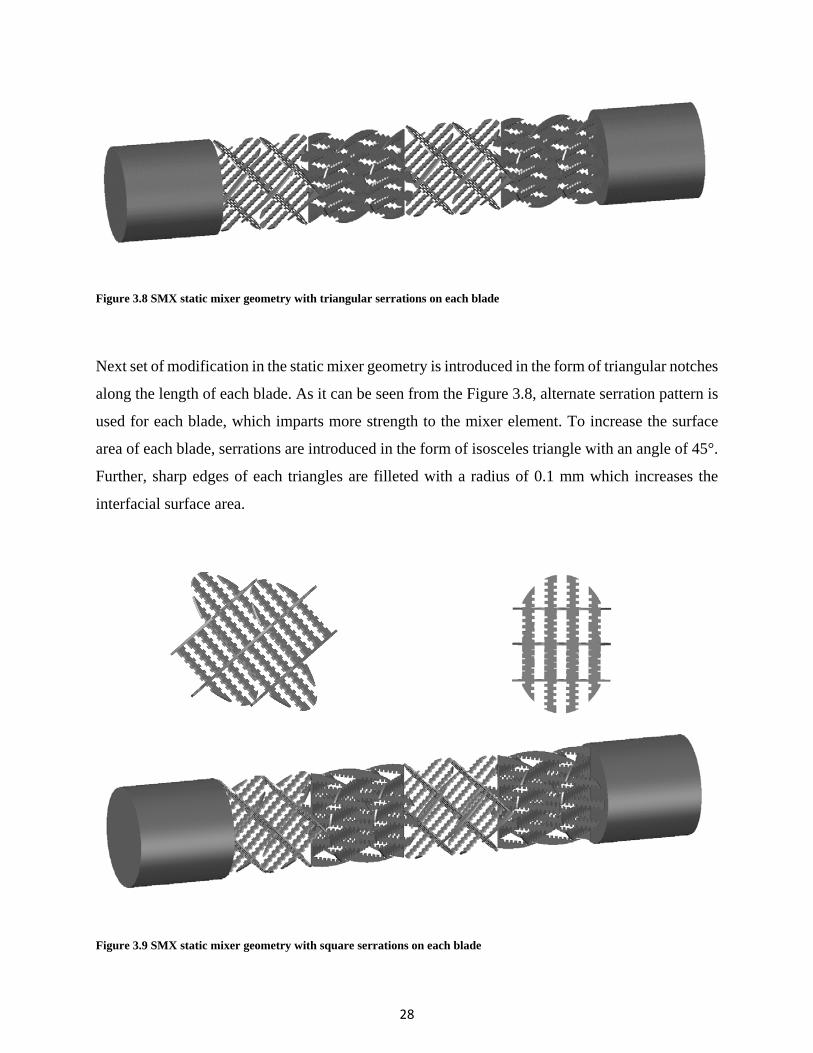
Figure 3.8 SMX static mixer geometry with triangular serrations on each blade
Next set of modification in the static mixer geometry is introduced in the form of triangular notches
along the length of each blade. As it can be seen from the Figure 3.8, alternate serration pattern is
used for each blade, which imparts more strength to the mixer element. To increase the surface
area of each blade, serrations are introduced in the form of isosceles triangle with an angle of 45°.
Further, sharp edges of each triangles are filleted with a radius of 0.1 mm which increases the
interfacial surface area.
Figure 3.9 SMX static mixer geometry with square serrations on each blade

29
Last design modification in the standard SMX geometry is done by introducing square shaped
serrations along the length. The dimension of each square is kept same as the radius of circular
serrations which is 1.315 mm. Since the sharp notches reduces the pressure of the flowing fluid
significantly, they are filleted by radius of 0.1 mm. Apart from increasing the interfacial surface
area, additional benefit of filleting the sharp edges would be ease of meshing the geometry in
COMSOL.
Dimensions of all static mixers have been shown in Table 3.1. For convenience, arrangement of 4
mixer elements inside the pipe is shown in all figures for the static mixers. However, all CFD
simulations are performed for the arrangement of 8 mixer elements inside the pipe.
Table 3.1 Dimensions of all static mixer geometries
Type of
geometry with
8 mixer
elements
Diameter of
element
(D) (mm)
Length of
pipe
(L)
(mm)
Thickness
of element
(mm)
Diameter
of Tube
(Dt)
(mm)
No. of
holes
per
element
Dimensions
of
perforations
/serrations
SMX 52.6 530 1 53 - -
Perforated
SMX 2 holes
52.6 530 1 53 64 2.63
Perforated
SMX 4 holes
52.6 530 1 53 120 2.63
Perforated
SMX
maximum
holes D/20
52.6 530 1 53 180 2.63
Perforated
SMX
maximum
holes D/30
52.6 530 1 53 288 1.753
30
Perforated
SMX
maximum
holes D/40
52.6 530 1 53 432 1.315
SMX with
circular
serrations
52.6 530 1 53 336 2.63
SMX with
triangular
serrations
52.6 530 1 53 744 2.5271
(base) and
45°
SMX with
square
serrations
52.6 530 1 53 580 1.315
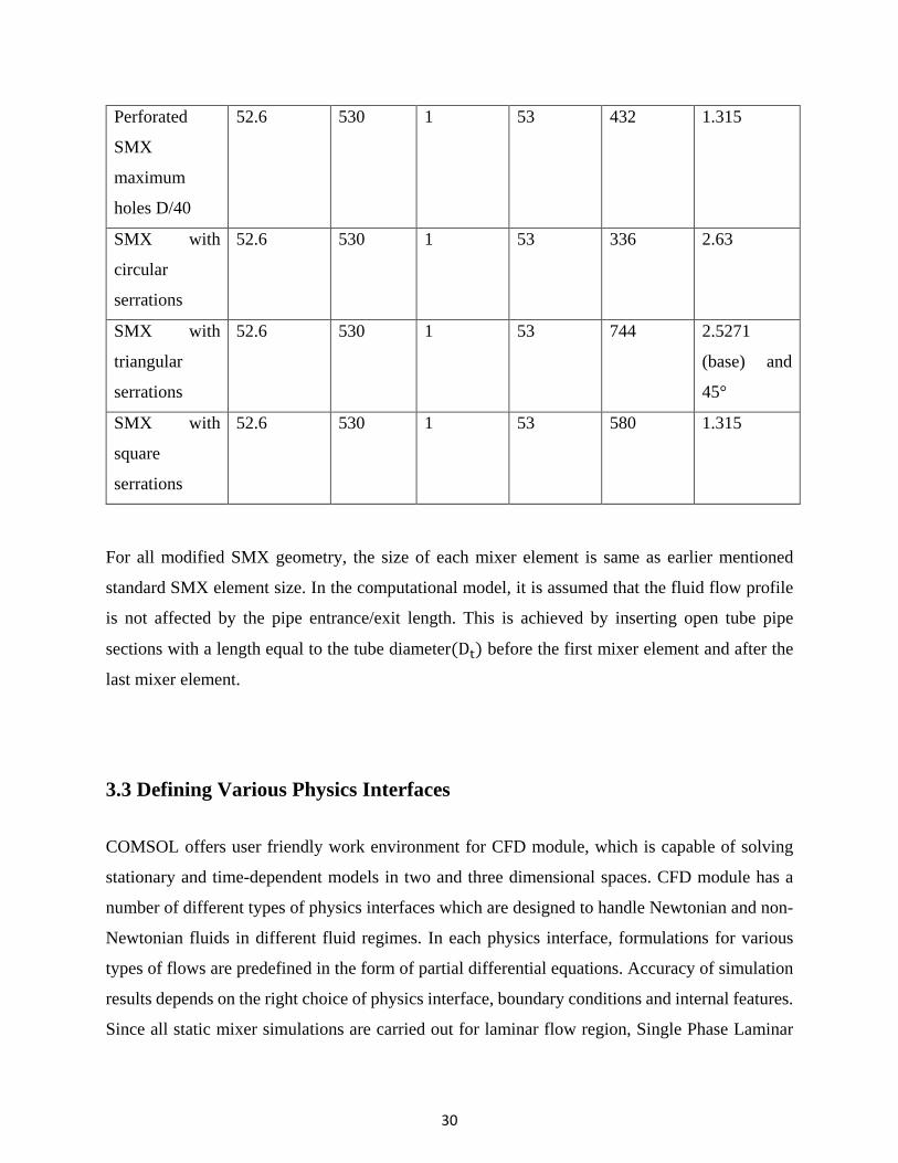
For all modified SMX geometry, the size of each mixer element is same as earlier mentioned
standard SMX element size. In the computational model, it is assumed that the fluid flow profile
is not affected by the pipe entrance/exit length. This is achieved by inserting open tube pipe
sections with a length equal to the tube diameter(Dt) before the first mixer element and after the
last mixer element.
3.3 Defining Various Physics Interfaces
COMSOL offers user friendly work environment for CFD module, which is capable of solving
stationary and time-dependent models in two and three dimensional spaces. CFD module has a
number of different types of physics interfaces which are designed to handle Newtonian and non-
Newtonian fluids in different fluid regimes. In each physics interface, formulations for various
types of flows are predefined in the form of partial differential equations. Accuracy of simulation
results depends on the right choice of physics interface, boundary conditions and internal features.
Since all static mixer simulations are carried out for laminar flow region, Single Phase Laminar

31
Flow Interface was used from the CFD module. This interface is built to solve equations for
conservation of momentum and equations for conservation of mass [48].
For a Newtonian fluid, the motion of fluids in a static mixer is governed by the Navier-Stokes (NS)
equation [49]. It can be seen as Newton’s second law of motion for fluids. For compressible fluids,
the general form of NS equation is shown by eq. (3.1) and (3.2),
ρ �∂u∂t
+u . ∇u� = (−∇p) + ∇. (τ) + (F)
(3.1)
ρCp �∂T∂t
+ (u.∇)T� = −(∇. q) + τ: S − Tρ∂ρ∂T
|p �∂p∂t
+ (u.∇)p� + Q (3.2)
Where u is the fluid velocity (SI unit: m/s), p (SI unit: Pa) is the fluid pressure, ρ (SI unit: kg/m3)
is the fluid density, τ is the viscous stress tensor (SI unit: Pa), F is the volume force vector (SI unit:
N/m3) and μ is the fluid dynamic viscosity (SI unit: Pa.s). The second equation represents
conservation of energy in terms of temperature. In this equation, T is the absolute temperature (SI
unit: K), S is the strain-rate tensor which is shown in equation (3.5), q is the heat flux vector (SI
unit: W/m2), Q is the heat source (SI unit: W/m3), Cp is the specific heat capacity at constant
pressure (SI unit: J/(kg.K)). The operation “:” implies the double dot product.
𝐚𝐚:𝐛𝐛 = ��𝐚𝐚𝐧𝐧𝐧𝐧𝐛𝐛𝐧𝐧𝐧𝐧𝐧𝐧𝐧𝐧
(3.3)
Since isothermal condition has been adopted in this study for all the static mixer simulations,
Eq.(3.2) can be decoupled from the NS equation. To solve equation (3.1), linear constitutive
relation between stress and strain is needed [50].
𝛕𝛕 = 𝟐𝟐𝟐𝟐𝟐𝟐 − 𝟐𝟐𝟑𝟑𝟐𝟐(𝛁𝛁.𝐮𝐮)𝐈𝐈 (3.4)

32
Strain rate tensor S can be written as
𝟐𝟐 = 𝟏𝟏𝟐𝟐
(𝛁𝛁𝐮𝐮 + (𝛁𝛁𝐮𝐮)𝐓𝐓) (3.5)
By replacing the values of τ and S in the Eq. (3.1), NS equation can be rewritten as:
ρ �∂u∂t
+u . ∇u����������1
= (−∇p)���2
+ ∇ . �µ(∇u + (∇u)T) − 23µ(∇ . u)I������������������������
3
+ (F)�4
(3.6)
The different terms correspond to the inertial forces (1), pressure forces (2), viscous forces (3),
and the external volume forces applied to the fluid (4).
These equations are always solved together with the continuity equation:
∂ρ∂t
+ ∇ . (ρu) = 0 (3.7)
The Navier-Stokes equations represent the conservation of momentum, while the continuity
equation represents the conservation of mass. In this study, water is selected as a working fluid.
Since water is incompressible, continuity equation reduces to
𝛁𝛁. (𝐮𝐮) = 𝟎𝟎 (3.8)
Due to this, divergence of velocity �− 23µ(∇ . u)I� from the viscous force term can be removed.
For all flow simulations time independent condition �∂u∂t
= 0� has been used. All these conditions
yield the NS equation in the final reduced form of
33
ρ(u . ∇u) = (−∇p) + ∇ . �µ(∇u + (∇u)T)� + F (3.9)
The NS equation along with the defined boundary conditions is solved within the fluid domain.
Since the main purpose of implementing Laminar Flow Interface was to obtain the velocity
profile and pressure fields, the only boundary conditions adopted are inlet and outlet conditions.
If several volume force nodes are added as additional boundary conditions, then their
contribution appears as ‘F’ on the right hand side of the momentum equation. In each case, since
the section of pipe consisting of static mixer is in horizontal position, the gravitational effects as
an external volume force can be neglected from the NS equation. For all the flow simulations,
no slip boundary condition is applied. This condition prescribes that the fluid at the wall is not
moving. The flow conditions are governed by the Reynolds number (Re), which is given by the
following equation.
𝐑𝐑𝐑𝐑 = 𝛒𝛒𝐮𝐮𝐃𝐃𝐭𝐭µ
(3.10)
Where, u is the average fluid velocity, ρ is fluid density, Dt is diameter of tube and µ is the dynamic
viscosity of fluid. Flow simulations are performed for a wide range of Reynolds numbers such as
0.0001, 0.001, 0.01, 0.1, 1, 10, 20, 30, 40, 50, 60, 70, 80, 90 and 100. Based on these Reynolds
numbers, the computed fluid velocity (u) is used as the inlet boundary condition to the fluid
domain. At the outlet, zero pressure (P=0) boundary condition is used.
Particle Tracing Interface
To analyze the overall performance of a static mixer, the evaluation of velocity profile and
pressure field is not sufficient. Though velocity and pressure field data are used to evaluate the
flow behavior of the static mixer, they do not give information about the distributive mixing
performance of the static mixer. Conventional experimental method requires to inject the tracer
of particles and track the movement of each particle in order to analyze the mixing of these
particles taking place along the length of the axis. In simulations, a similar approach is being
used and mixing ability of static mixer is visualized by incorporating the Particle Tracing

34
module. Particle Tracing interface is used to compute the motion of particles in the presence of
a flowing fluid. This dedicated physic interface is not only used to trace the trajectories of
particles but it also provides a Lagrangian description of a problem by solving ordinary
differential equations (ODE) using Newton’s law of motion [51].
The particle tracing interface works on Newton’s law of motion, when Newtonian particles are
selected in the corresponding module. It requires specification of the particle mass and the forces
acting on the particles. Generally the forces acting on it can be categorized into external field
force and particle-particle interaction force. However in the current study, as such no charged
particles have been used, the particle-particle interaction force can be neglected from the
computation. ODEs are solved for each particle and for each position vector component. It means
that it requires three ODEs for three dimensional geometry and two ODEs for two dimensional
fluid domain to be solved. At each time step, the position of each particle is computed by taking
into account different forces of external fields. Current position of particle is then updated and
it continues to repeat this process until the specified time in the simulation is reached.
Since the particles are injected in the existing flow field, it is important to confirm that particles
would not have a major impact on it. This limits the flexibility of application of Particle Tracing
Interface. Due to this reason, flow field is first computed using Laminar Flow Interface and then
the motion of particles are calculated as a secondary analysis step. The velocity of a particle is
given by Newton’s second law [51] which is shown in eq. (3.11)
𝐧𝐧𝐝𝐝𝟐𝟐𝒙𝒙𝐝𝐝𝐭𝐭𝟐𝟐
= 𝑭𝑭(𝐭𝐭,𝒙𝒙, 𝐝𝐝𝒙𝒙𝐝𝐝𝐭𝐭
) (3.11)
Where x is the position of the particle, m is the particle mass and F is the sum of all forces acting
on the particle. Different types of force which may act on the particles are the drag force, the
external volume force (Fext) like buoyancy and the gravity force (Fg). In this study, for each
simulation only the drag force have been taken into consideration. As the pipe is in horizontal
position and there are no other external forces, Fext and Fg are neglected. In other words,
Newton’s second law can be interpreted as the net force on a particle is equal to its time rate of
change of its linear momentum in an inertial reference frame. It can also be represented as
ddt�mpv� = FD + Fg + Fext
(3.12)

35
Where, FD represents the Drag Force, which is the force exerted by fluid on the particle due to
velocity difference between fluid and particle. There are several expressions which have been
suggested for the drag force. Among all, the one which is formulated for viscous drag force in
this physics interface is given by eq. (3.13):
FD = � 1τp�mp(u − v) (3.13)
Where mp is the particle mass (SI unit: kg), τp is the particle velocity response time (SI unit: s),
v is the velocity of the particle (SI unit: m/s) and u is the fluid velocity (SI unit: m/s). The particle
velocity response time (τp) for spherical particles in laminar flow is defined as:
τp = ρpdp2
18µ (3.14)
Where μ is the fluid viscosity (SI unit: Pa s), ρp is the particle density (SI unit: kg/m3) and dp is
the particle diameter (SI unit: m). This is frequently known as Stokes drag law. The particle
density is normalized in such a way that more number of particles were injected where the inlet
velocity is maximum and less number of particles were released in the region of low velocity
field. Particle Tracing Interface also includes some default boundary conditions like wall
conditions and particle properties. For all simulations, microscale Newtonian particles of
diameter 5x10⁻⁷ (m) were used. The density of particles used was 2200 (kg/m3).
The wall boundary condition is set to freeze for all the simulations. It implies that the moment
particles strike the wall, their position no longer changes and velocity becomes a constant value.
Since Newtonian spherical particles have been used in all simulations, all of them do not
necessarily reach at the outlet of the pipe. Because of the preset wall condition and mass of the
particles, some of these particles get stuck on the boundary of the walls and on the mixer
elements. Due to this, instead of taking into account the coefficient of variation (COV), mixing
of particles was measured in terms of gradual decrease in the standard deviation along the length
of the reactor.

36
3.4 Meshing
Once the simulation model is set up, the next important step is to build a mesh. Numerical mesh
generation is the result of discretization of CAD geometry. Effective simulation results depend
on the size of an individual mesh element and the distribution pattern of mesh. Defining various
physics interface in the model is seen as creating an operation node, which in turn builds or
modifies the mesh on the CAD geometry. Creating a mesh sequence results into attributing
various nodes to a corresponding geometry. The properties defined by different physics
interfaces are stored in these attributed nodes. To discretize the CAD model, the first step is to
remove the irrelevant details and make the geometry as simpler as possible for an ease of
meshing. In this study, as different set of three dimensional geometries of static mixers are used,
it is necessary to remove the defects of geometries. By introducing smaller sized perforations
and serrations to the SMX geometry, the degree of complexity is increased which in turn requires
more refined mesh and thereby more computer resources and computational time is required to
simulate the model. These geometries were refined using composite faces and by ignoring some
minor edges for an ease of meshing.
In order to compute velocity and pressure profiles, the flow domain is subdivided into number
of small, regular and connected finite elements [52]. Mesh elements can be triangles,
quadrilaterals, tetrahedral or polyhedral. Conventionally, 1D geometries are discretized in mesh
vertices, while 2D geometries are discretized in triangular or quadrilateral mesh elements. For
3D geometry, the flow domain can be subdivided into tetrahedral, hexahedral, prism, or pyramid
mesh elements [53]. As for all the simulations default mesh sequence of COMSOL is used, the
static mixer geometry is subdivided into small elements of geometrically much simpler shapes
such as tetrahedrons. The distribution density of default size mesh follows the physics of the fluid
flow very closely. The grid density is finer where the flow conditions are changing rapidly and
have a larger gradients, whereas the grid is coarser where the flow conditions are constant and
have smaller gradients. The final mesh used for 3D SMX geometry contained 419276 tetrahedral
elements composed of 2792 vertexes. Total mesh volume is 1118000 mm3 with an element volume
ratio of 4.784 x 10⁻⁶. The average growth rate of mesh elements is 2.475 and it attains the maximum
value of 22.68. As the extent of complexity increases, the number of tetrahedral elements needed
to subdivide the flow domain increases significantly. SMX geometry of D/40 size perforations is

37
discretized into 4330377 tetrahedral elements, which is approximately ten times more than normal
SMX geometry.
Once the model geometry has been discretized in this pattern, the values of velocity components
and pressure field are being evaluated at each node of the meshed geometry by using an inbuilt
solver of COMSOL.
3.5 Solvers
Once the model is setup and geometry is meshed, a robust solver is needed to solve and obtain the
computational results. Fluid flow characteristics in the laminar regime and mixing of particles in
various static mixers were evaluated in two steps. In the first step, velocity profile and pressure
fields were computed using the information given in Laminar Flow Interface. The second step
involves the information of Particle Tracer Interface to compute the particle trajectory and hence
the mixing of particles. In this study, to perform each simulation, fully coupled, finite element
based nonlinear solver has been used. The first step of solver configuration involves the use of
Navier-Stokes equations to compute the dependent variables (velocity field and pressure) of the
system. Since NS equation constitutes nonlinear system of equations, default non-linear stationary
solver settings have been used. The default solver settings for fluid flow interfaces are optimized
to handle wide range of flow conditions. The nonlinear solver adopts Newton-Raphson iteration
scheme and in each iteration, a linearized version of nonlinear system is solved to reach the final
solution. The values of pressure and velocity field computed by the first step, were used as initial
values to solve particle trajectories in the second step. In this step, particle velocities were
computed using a time-dependent nonlinear solver.
The selection of solver totally depends on what type of physic interface is involved in the model.
Default finite element method based solvers work adequately well without giving any errors.
However, due to the complexity of geometries, direct solution method was used instead of default
iterative solution method for nonlinear solver configuration. Direct solution method is more robust
compared to iterative method. Due to the complexity of the geometries, model could not converge
with iterative method.

38
3.6 Conclusion
Complete methodology of setting up a CFD model in COMSOL has been discussed in this chapter.
Different static mixer geometries designed in AutoCAD, were imported to COMSOL environment
and the computational model was setup using various physics interface. The geometries were
discretized in smaller tetrahedron elements and properties of physic interface were attributed to
geometry nodes. A finite element method based non-linear solver was used to simulate the model
numerically. The governing nonlinear equations for the flow of fluid in laminar flow regime and
the particle motion equations were solved in the two steps. The velocity and pressure field values
computed in the first step were used to calculate particle motion in the second step.

39
CHAPTER 4: Laminar Mixing in static mixers
4.1 Introduction
Numerical results of the CFD model for previously mentioned different static mixer geometries
are presented in this chapter. As discussed in Chapter 3, multiphysics computational model using
laminar flow interface and particle tracing interface is setup in COMSOL to analyze the mixing
capacity of all SMs. For all the simulations, inlet conditions and input model parameters used for
different static mixer geometries are shown in Table 4.1. It should be noted that all SM geometries
are simulated for Reynolds number ranging from 0.001 to 100. All the parameters shown in Table
4.1 will be same except velocity, which is computed accordingly with the varying Reynolds
number. In Table 4.1, velocity is computed for Re 30.
Table 4.1 Inlet conditions and input parameters used for all static mixer geometries
Model Inputs Value
Laminar Flow Interface Density of working fluid 1000 (kg/m3)
Viscosity of working fluid 0.001 (Pa.s)
Inlet velocity 5.6603 × 10⁻⁴ (m/s)
Outlet pressure 0 (Pa)
Particle Tracing Interface No. of particles 5000
Diameter of particle 5 × 10⁻⁷ (m)
Particle density 2200 (kg/m3)
Once the model is simulated it is important to compare the numerical results with experimental
data, in order to validate the reliability of the CFD model. There are couple of parameters available
in the literature, which have been used by several research groups to measure the overall
performance of static mixers. In this study, different parameters for dispersive mixing and
distributive mixing are selected to quantify the static mixer performance. This chapter is basically
divided into two parts. In the first part, different parameters used to compare the dispersive mixing

40
quality of all the static mixers is discussed. These include pressure drop, velocity field, shear rate
and extensional efficiency. Simulation results are shown in terms of line plots and visual contour
plots. In the second part, distributive mixing capacity of all the static mixers have been discussed
in terms of the standard deviation. To analyze the mixing taking place inside a static mixer element,
a binary mixture of coloured particle tracer has been used. Progressive distributive mixing of red
and blue coloured particles can be visualized in terms of contour plots. Based on the comparison
of these factors, the best static mixer deign has been suggested for polymerization of acrylamide.
4.2 Characteristics of Flow Field in different static mixers
As mentioned in the Chapter 3, different SMs used to characterize the flow field are SMX,
perforated SMX with 2 holes on each blade, perforated SMX with 4 holes on each blade, perforated
SMX with hole size D/20, perforated SMX with hole size D/30, perforated SMX with hole size
D/40, SMX with circular serrations, SMX with triangular serrations and SMX with square
serrations. In COMSOL, these geometries are imported and aligned in the XY plane such that the
X direction becomes predominantly the flow direction of the fluid. Center line of the pipe having
static mixer element, lies on the coordinate (y, z) = (0.0265, 0.0265) and extends from x = 0 to x
= 0.053 m. Since water has been selected as a working fluid, the density and viscosity are 1000
(kg/m3) and 0.001 (Pa.s) respectively. In each simulation, the velocity of fluid computed from
Reynolds number ranging from 10-4 to 100 was applied respectively to the inlet of the pipe. For
each simulation, zero pressure condition (P = 0) has been used at the outlet of the pipe. Once the
model is setup simulations are performed in two steps: First step giving flow field simulation
results and second step giving particle tracer results. Each simulation took on an average of 10
hours to converge when running in parallel on a 3.6 GHz core i7-4790 CPU.
In this section, flow field results obtained from simulations are first evaluated in terms of Z factor,
pressure field contours and velocity contours. The flow field results are further characterized using
different parameters to analyze the ability of static mixers in terms of dispersive mixing. There are
different parameters such as shear rate (γ), extensional efficiency (eλ), deformation tensor,
stretching (λ) and Lyapunov exponent (δ), which are used by former research groups to evaluate

41
the dispersive mixing of SMs [37]. However in the current study, only shear rate and extensional
efficiency are used to evaluate the dispersive mixing characteristics.
4.2.1 Pressure Drop
Pressure drop is an important criterion, which is used in industries to analyze the performance of
a static mixer. It is also being used as a tool to validate the reliability of the CFD model. Since the
pressure drop is directly related to the loss of supplied energy, it is always desired to minimize the
pressure drop in a static mixer.
In all simulations, zero pressure condition (P=0) is adopted at the outlet of the pipe. The difference
between the pressure values evaluated at 0.1 cm upstream of the first mixer element and 0.1 cm
downstream of last mixer element is defined as the pressure drop imposed by the static mixer.
Particularly in this study, pressure drop is computed across the eight mixer elements. In the
literature data, pressure drop correlations are presented in three different ways: 1) pressure drop
(∆P) 2) pressure drop ratio (Z) and 3) friction factor (f/2). In this work, to compare the numerical
results with an experimental data, pressure drop (∆P) and pressure drop ratio (Z) have been taken
into consideration. The pressure drop ratio or Z factor is defined as
Z = ∆PSM∆PET
(4.1)
Where ∆PSM is the pressure drop within the static mixer, while ∆PET corresponds to empty tube
pressure drop. The results of the pressure drop ratio (Z) vs Re and static mixer pressure drop
(∆PSM) vs Re are shown in the Figure 4.1 and Figure 4.2 respectively. As shown in the Figure 4.1,
Z factor is almost independent from the variations of Reynolds number (Re) till it reaches the value
of 10. As the inertial effects are insignificant for low flow values, the pressure drop ratio Z is
constant till Re < 10. However, the Z factor increases non-linearly with the Reynolds number
increasing from 10 to 100. Computed Z values are compared with the literature data, which shows
the same trend for the variation of Z values for Re > 10. For SMX static mixer, the Z value is
41.28877 for Re < 10 and it reaches up to 46.9401 for Re = 100. These values are within the same
range specified by Pahi and Muschelknautz [54]. According to Pahi and Muschelknautz, Z factor

42
values may vary from 10 to 60 for SMX static mixer. A study performed by Alloca (1982) [55],
suggested that the value of Z should be 38.7 for Re < 10. In the current study, the value of Z is
41.28877 which is closer to the reported values.
Figure 4.1 Comparison Plot of Pressure Drop Ratio (Z) vs Reynolds number (Re) for all static mixer geometries for Reynolds number 0.0001 to 100.
In Figure 4.2, variation of the pressure drop (∆P) with increasing Reynolds number is shown. Since
the applied inlet velocities are very low for Reynolds number ranging from 10-4 to 1, the entire
flow domain is working at a very low pressure. Due to this, the pressure drop values are very low
and not clearly visible in the plot for Re < 10. For the Reynolds number > 10, the pressure drop
increases continuously due to an increase in inertial effects, shear force and frictional losses. As
shown in Figure 4.2 , by increasing the number of holes of size D/20, the pressure drop decreases.
However, by decreasing the size of hole from D/20 to D/40, the mixing performance is deteriorated
and pressure drop increases. In fact, SMX geometry with perforations of D/40 size, gives almost
same or sometimes higher pressure drop than standard SMX. Among all perforated geometries,
SMX geometry with maximum number of D/20 holes demonstrates minimum pressure drop,
which is almost 27-28% lesser than the pressure drop imposed by standard SMX geometry.
Perforations of size D/20 reduces the pressure drop significantly. However, it is not as good as
SMX geometry with circular serrations. SMX geometry with circular serrations impose 36-37%
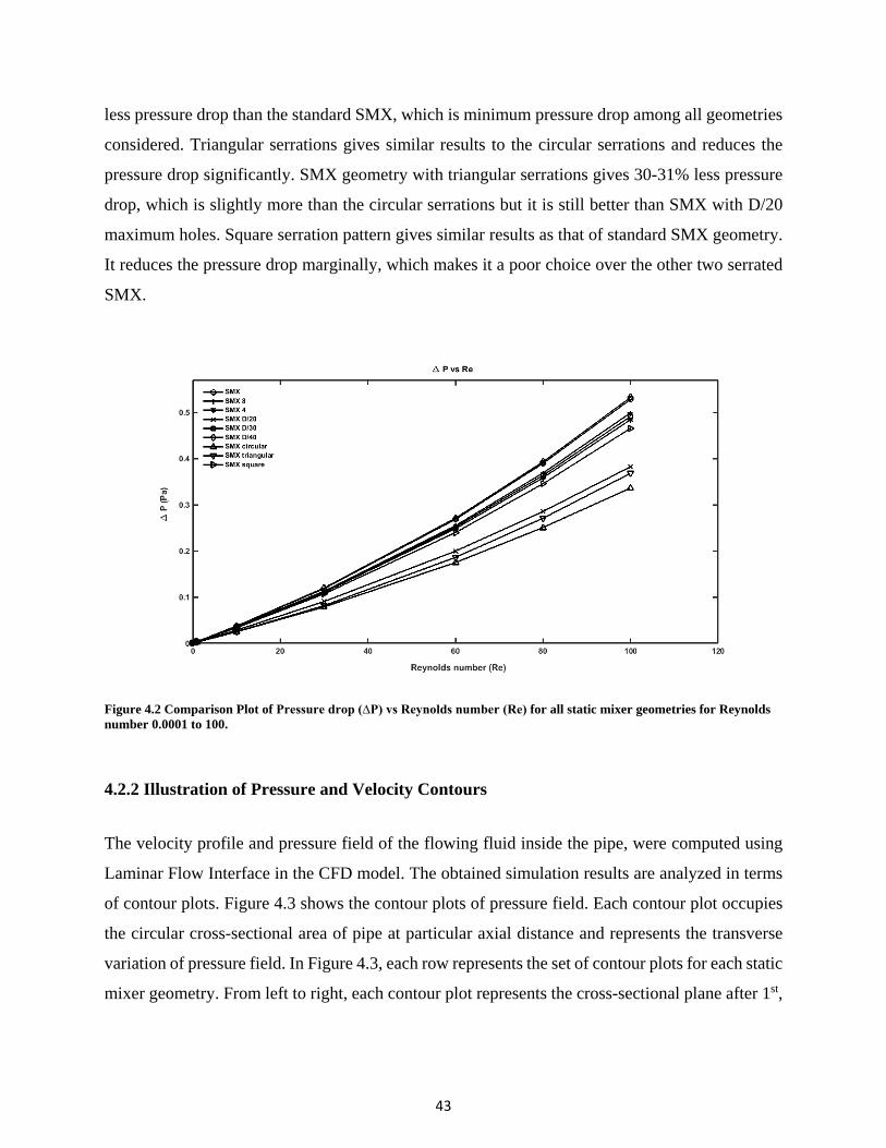
43
less pressure drop than the standard SMX, which is minimum pressure drop among all geometries
considered. Triangular serrations gives similar results to the circular serrations and reduces the
pressure drop significantly. SMX geometry with triangular serrations gives 30-31% less pressure
drop, which is slightly more than the circular serrations but it is still better than SMX with D/20
maximum holes. Square serration pattern gives similar results as that of standard SMX geometry.
It reduces the pressure drop marginally, which makes it a poor choice over the other two serrated
SMX.
Figure 4.2 Comparison Plot of Pressure drop (∆P) vs Reynolds number (Re) for all static mixer geometries for Reynolds number 0.0001 to 100.
4.2.2 Illustration of Pressure and Velocity Contours
The velocity profile and pressure field of the flowing fluid inside the pipe, were computed using
Laminar Flow Interface in the CFD model. The obtained simulation results are analyzed in terms
of contour plots. Figure 4.3 shows the contour plots of pressure field. Each contour plot occupies
the circular cross-sectional area of pipe at particular axial distance and represents the transverse
variation of pressure field. In Figure 4.3, each row represents the set of contour plots for each static
mixer geometry. From left to right, each contour plot represents the cross-sectional plane after 1st,
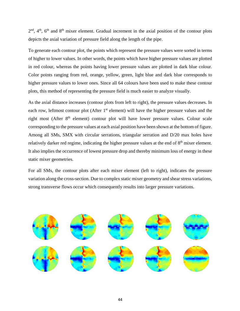
44
2nd, 4th, 6th and 8th mixer element. Gradual increment in the axial position of the contour plots
depicts the axial variation of pressure field along the length of the pipe.
To generate each contour plot, the points which represent the pressure values were sorted in terms
of higher to lower values. In other words, the points which have higher pressure values are plotted
in red colour, whereas the points having lower pressure values are plotted in dark blue colour.
Color points ranging from red, orange, yellow, green, light blue and dark blue corresponds to
higher pressure values to lower ones. Since all 64 colours have been used to make these contour
plots, this method of representing the pressure field is much easier to analyze visually.
As the axial distance increases (contour plots from left to right), the pressure values decreases. In
each row, leftmost contour plot (After 1st element) will have the higher pressure values and the
right most (After 8th element) contour plot will have lower pressure values. Colour scale
corresponding to the pressure values at each axial position have been shown at the bottom of figure.
Among all SMs, SMX with circular serrations, triangular serration and D/20 max holes have
relatively darker red regime, indicating the higher pressure values at the end of 8th mixer element.
It also implies the occurrence of lowest pressure drop and thereby minimum loss of energy in these
static mixer geometries.
For all SMs, the contour plots after each mixer element (left to right), indicates the pressure
variation along the cross-section. Due to complex static mixer geometry and shear stress variations,
strong transverse flows occur which consequently results into larger pressure variations.

45
(a) (b) (c) (d) (e)
Figure 4.3 Comparison of Pressure field contour plots (Pa.S) for all static mixer geometries at Re = 30.

46
(a) After 1st mixer element (b) After 2nd mixer element (c) After 4th mixer element (d) After 6th mixer element (e) After last mixer element. From top to bottom each row represents the contour plots for the following geometries: SMX, Perforated SMX, Perforated SMX 4 holes, Perforated SMX maximum no. of D/20 holes, Perforated SMX maximum no. of D/30 holes, Perforated SMX maximum no. of D/40 holes, SMX with circular serrations, SMX with triangular serrations and SMX with square serrations.
Velocity profile of the flowing fluid is another important quantity which reveals the flow behavior
of fluid within the static mixer elements. Figure 4.4 shows the contour plots of velocity of the
flowing fluid within the SM elements. Analogous to the pressure field contour plots, the same
colour scale has been used to illustrate the velocity profile i.e. red colour points represent higher
velocity values, while dark blue colour points represent the lower velocity values. Another analogy
to the pressure contour plots is, each row demonstrates a particular set of contour plots for each
static mixer and represents axial and transversal variations of velocity.
At inlet, flat velocity profile has been incorporated, which rapidly develops into parabolic velocity
profile with the highest velocity values at the center. It can be seen from the contour plots that, as
the fluid moves forward and strikes the first element, division of flow occurs and the parabolic
velocity profile is split into four cores. By comparing the pressure contour plots and velocity
contour plots, it is apparent that as the fluid moves along the length of the pipe, due to continuous
splitting, rotation and stretching, it gains higher velocity at the cost of higher pressure loss. The
variation in fluid velocity also depends on the shape of the geometry. It is always desirable to have
uniformly distributed velocity profile and less variations in transverse velocity at each cross
sectional plane. Contour plots after the 8th mixer element illustrate that circular serrations gives
better results in terms of velocity distribution. The colour difference across the center line is less,
which represents less variation in transverse velocity. Whereas, perforations of size D/20 and
triangular serrated SMX, show more transverse velocity variations.
The data obtained from the simulation results shows that SMX has the highest volume average
velocity than other SMs. Further, as the perforation size decreases from D/20 to D/30 and D/40,
the performance of SM gets deteriorated. Circular SMX gives minimum volume average velocity,
while triangular serrated SMX and D/20 perforated SMX give slightly higher volume average
velocity than circular serrated SMX. Square serrated SMX shows the highest volume average
velocity among all. In the next section, shear rate and extensional efficiency have been discussed
to understand the flow field characteristics and the dispersive mixing taking place in the SM.
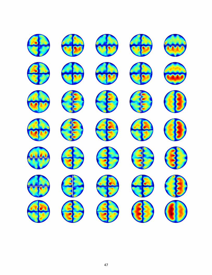
47
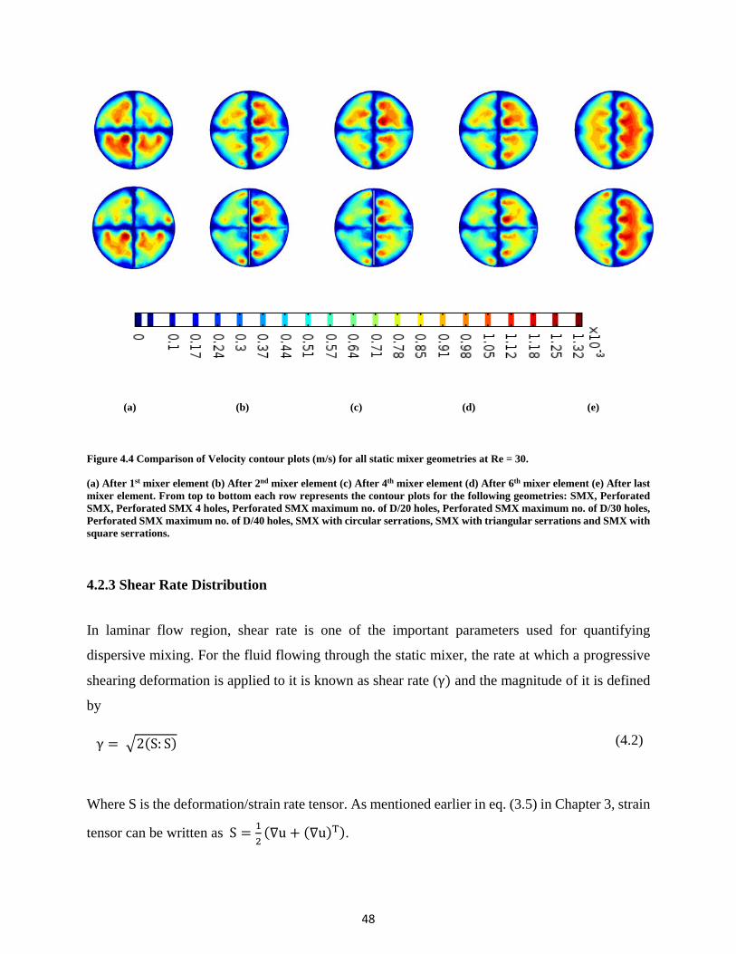
48
(a) (b) (c) (d) (e)
Figure 4.4 Comparison of Velocity contour plots (m/s) for all static mixer geometries at Re = 30.
(a) After 1st mixer element (b) After 2nd mixer element (c) After 4th mixer element (d) After 6th mixer element (e) After last mixer element. From top to bottom each row represents the contour plots for the following geometries: SMX, Perforated SMX, Perforated SMX 4 holes, Perforated SMX maximum no. of D/20 holes, Perforated SMX maximum no. of D/30 holes, Perforated SMX maximum no. of D/40 holes, SMX with circular serrations, SMX with triangular serrations and SMX with square serrations.
4.2.3 Shear Rate Distribution
In laminar flow region, shear rate is one of the important parameters used for quantifying
dispersive mixing. For the fluid flowing through the static mixer, the rate at which a progressive
shearing deformation is applied to it is known as shear rate (γ) and the magnitude of it is defined
by
γ = �2(S: S) (4.2)
Where S is the deformation/strain rate tensor. As mentioned earlier in eq. (3.5) in Chapter 3, strain
tensor can be written as S = 12
(∇u + (∇u)T).

49
As shown in the Figure 4.5, fluid velocity contours obtained from the simulation results can be
used to illustrate the bulk flow pattern. However, local mixing rates are determined by the
magnitude of deformation tensor. Deformation/strain rate tensor represents straining motion of
fluid element due to the existing shear stress field.
Since an actual fluid resists the shear exerted by an upper layer of the fluid, a shear force (Fs) is
generated in the shear stress field. The quantity ‘Shear Stress’ is used to represent the shear stress
field, which is defined as the shear force (Fs) acting per unit area of the shearing plane (As).
Shear Stress = (Fs / As)
If the shear stress is arising from the viscous or laminar flow, it is denoted by εv. For the Newtonian
fluid, viscous shear stress (εv) is related to shear rate (γ) by εv=µγ.
One implication from the relationship between shear stress and shear rate is that, as the shearing
plane area decreases the rate of shear and the viscous shear stress increases. Increase in shear rate
and viscous stress results into more dispersive mixing of the fluid. This phenomenon is observed
when the fluid flows through the static mixer and gives more shear rate as compared to the flow
in an empty pipe. One disadvantage of higher shear stress is, more energy of fluid stream is lost in
terms of pressure. To assess the dispersive mixing capacity of static mixers, shear rate distribution
at several cross-sectional planes in the first mixer elements is shown in the Figure 4.5. For each
static mixer, these cross-sectional planes are located in the first mixer element at a distance of
(D/4), (3D/8), (D/2) and D. Where, D is the diameter of mixer element.
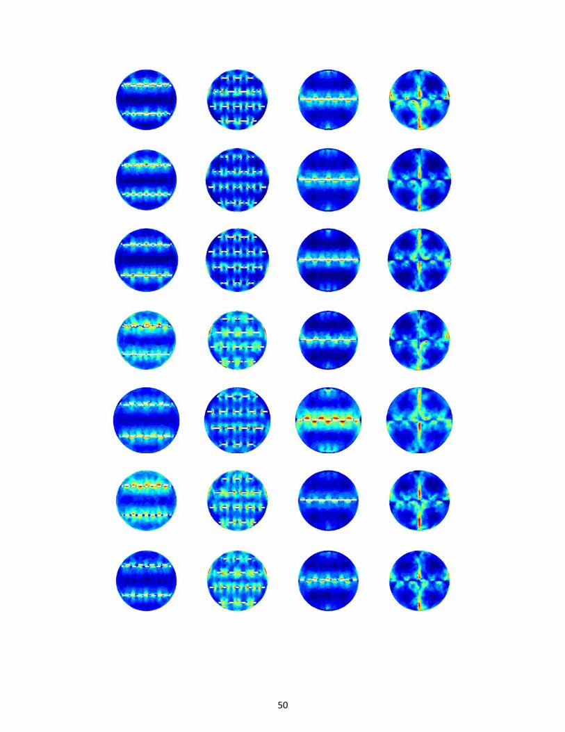
50

51
(a) (b) (c) (d)
Figure 4.5 Comparison of Shear rate vs Reynolds number contour plots for all static mixer geometries at Re = 30.
(a) At D+(D/4) distance from inlet (b) At D+(3D/8) distance from inlet (c) At D+(D/2) distance from inlet (d) At 2D distance from inlet. From top to bottom each row represents the contour plots for the following geometries: SMX, Perforated SMX, Perforated SMX 4 holes, Perforated SMX maximum no. of D/20 holes, Perforated SMX maximum no. of D/30 holes, Perforated SMX maximum no. of D/40 holes, SMX with circular serrations, SMX with triangular serrations and SMX with square serrations.
These contour plots indicate that the shear rate distribution in SMs is very non-uniform. Relatively
low shear rates occur when the cross blades are sparse. On the other hand, high shear rate zones
are located around the cross-blades. High shear rate zones have the greatest potential of fluid
elements getting stretched and dispersed but they impose higher pressure drop. As the fluid moves
forward, it is observed that shear rates vary within cross-sectional area indicating varying
dispersive mixing. These contour plots give information about the transverse and axial shear rate
distribution. However, it does not give any information about the mean shear rate in the flow
domain. Local spatial derivatives of the velocity components have been computed in the flow field
simulations. Local velocity gradients allow us to determine the local shear rates and mean shear
rates. Figure 4.6 shown below gives variation in the mean shear rate with Reynolds number.
It is evident that standard SMX impose highest mean shear rate, while the circular and triangular
serrated SMX impose much lower shear rate. Circular and triangular serrations give almost same
mean shear rate with increasing Reynolds number. Square serrations gives similar results as SMX
geometry. Perforated D/20 SMX gives slightly lower mean shear rate than SMX, but higher shear
rate values than the circular and triangular serrations. By comparing the, shear rate vs Re plot to
the pressure drop vs Re plot, it is apparent that higher shear rate leads to higher pressure drop. This
direct relation between pressure drop and shear rate is quite logical since the power lost by friction
of volume V is:
Q.∆P = ∭τ: γ dV (4.3)

52
Where τ is stress tensor. This relation shows how pressure drop or energy consumption is
transformed into shear stress. The volume of the flow domain in each case is roughly the same
� τ∆P� and is inversely proportional to the shear rate (γ) [33]. This relation is confirmed from the
simulation results of shear rate and pressure drop variations. Circular serrated SMX imposed
lowest pressure drop, which results into minimum shear rate among all SMs. The same is true for
standard SMX mixer which shows maximum shear rate and has highest pressure drop.
Figure 4.6 Comparison plots of Shear rate (γ) vs Reynolds number for SMX, Perforated SMX D/20 maximum number, SMX with circular serrations, SMX with triangular serrations and SMX with square serrations static mixers.
4.2.4 Extensional Efficiency
Apart from shear rate distribution, another important parameter used to quantify the dispersive
mixing is extensional efficiency. Dispersive mixing depends on the occurrence of different types
of flow inside the static mixer. In an empty pipe flow where no physical impedance is present for
the flow of fluid, simple shear flow occurs. While the flow of fluid inside the static mixer element,
fluid stream gets rotated, twisted and stretched continuously. This type of motion of fluid causes
shear flow, elongational flow and squeezing flow depending on the mixer geometry and the
extensional efficiency. Each of these flows has different mixing behavior. For infinitesimally small
fluid element, elongational flow always tends to attain the maximum specific stretching rate. On
the contrary, simple shear flow always tends to make specific stretching rate zero and causes the
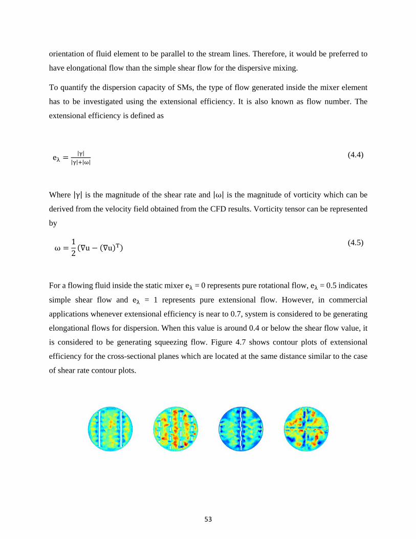
53
orientation of fluid element to be parallel to the stream lines. Therefore, it would be preferred to
have elongational flow than the simple shear flow for the dispersive mixing.
To quantify the dispersion capacity of SMs, the type of flow generated inside the mixer element
has to be investigated using the extensional efficiency. It is also known as flow number. The
extensional efficiency is defined as
eλ = |γ||γ|+|ω|
(4.4)
Where |γ| is the magnitude of the shear rate and |ω| is the magnitude of vorticity which can be
derived from the velocity field obtained from the CFD results. Vorticity tensor can be represented
by
ω =12
(∇u − (∇u)T) (4.5)
For a flowing fluid inside the static mixer eλ = 0 represents pure rotational flow, eλ = 0.5 indicates
simple shear flow and eλ = 1 represents pure extensional flow. However, in commercial
applications whenever extensional efficiency is near to 0.7, system is considered to be generating
elongational flows for dispersion. When this value is around 0.4 or below the shear flow value, it
is considered to be generating squeezing flow. Figure 4.7 shows contour plots of extensional
efficiency for the cross-sectional planes which are located at the same distance similar to the case
of shear rate contour plots.
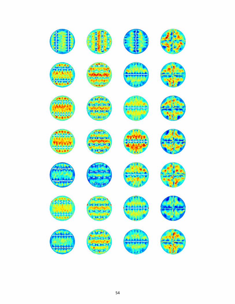
54

55
(a) (b) (c) (d)
Figure 4.7 Comparison of Extensional efficiency contour plots for all static mixer geometries at Re = 30.
(a) At D+(D/4) distance from inlet (b) At D+(3D/8) distance from inlet (c) At D+(D/2) distance from inlet (d) At 2D distance from inlet. From top to bottom each row represents the contour plots for the following geometries: SMX, Perforated SMX, Perforated SMX 4 holes, Perforated SMX maximum no. of D/20 holes, Perforated SMX maximum no. of D/30 holes, Perforated SMX maximum no. of D/40 holes, SMX with circular serrations, SMX with triangular serrations and SMX with square serrations.
It is evident from the contour plots that all three types of flows occur within the flow field of all
the SMs. It is also implied from the contour plots that, ‘X’ shape cross-blade produces the
elongational and squeezing flow. As the fluid moves across the cross joint, transition of flow
occurs from elongational flow to squeezing flow or vice versa. It gives an insight about the
occurrence of different types of flows and potential dispersion zones inside the mixer element.
However, it does not give information about the overall extensional efficiency of static mixer. The
plot of mean extensional efficiency with varying Reynolds number for SMs has been shown in
Figure 4.8.
As the Reynolds number increases, due to increasing inertial effects, elongational flow inside the
SMs decreases and extensional efficiency decreases for all the SMs. Standard static mixer gives
the lowest extensional efficiency, while circular serrated SMs has highest capability of generating
elongational flows. Perforated SMX of D/20 holes shows better extensional efficiency than
triangular serrations. It must be noted that the geometry of static mixer plays a vital role in creating
elongational flow. It is possible that the geometry having highest shear rate cannot necessarily
generate better elongational flow. The elongational flow represents the convergent characteristics
of flow, while squeezing flow shows divergent characteristics. It is desirable to have transition of

56
elongational flow to squeezing flow across the ‘X’ cross joints, to achieve effective dispersion. To
break and disperse the fluid element, elongational flows are necessary. Circular serrations shows
good transition of flow across the cross-blades and generates more elongational flows in the flow
domain. Due to this, extensional efficiency of circular serrated SMX is better than the normal SMX
at any given Reynolds number.
Figure 4.8 Comparison of Extensional efficiency vs Reynolds number (Re) contour plots for SMX, Perforated SMX D/20 maximum number, SMX with circular serrations, SMX with triangular serrations and SMX with square serrations static mixers.
4.3 Intensity of segregation
In this section, the distributive capacity of all SMs has been analyzed. Distributive mixing refers
to spatial distribution of the components throughout the flow domain. It is also known as simple
or extensive mixing. Compared to the dispersive mixing, this is much easier to achieve. Statistical
measure ‘Intensity of Segregation’ has been used to compare the distributive mixing capabilities
of all the static mixers. For this purpose, a cubic cluster of 5000 particles of two different colours
has been launched first at the center of the inlet of pipe �Z = Dt2�. Each particle has a diameter of
5x10⁻⁷ [m] and has no cohesion force with other particles. This means, the tracer of particles do

57
not affect the flow of field of the fluid but it rather represents the flow of fluid inside the static
mixer. The initial velocity of the particles is proportional to the fluid velocity. For particle tracing
and distributive mixing, massless particles are usually used. However, due to certain limitations of
the Particle Tracing Interface in COMSOL, Newtonian particles have been used in this work. The
particle trajectory in the flow field was computed using the Newtonian formulation as mentioned
in Chapter 3. Since the particles have mass, all of the released particles do not necessarily reach
the outlet of the flow domain; some of them get stuck inside the static mixer blades. The same
limitation prohibits to use the coefficient of variation (COV) measure. In most of the previous
literature work distributive mixing has been quantified in terms of COV; which is defined as:
COV =�∑ �Ni−N��
2ncellsi=1
ncells
N�
(4.6)
Where, Ni is the number of particles falling in ith grid cells and N� is the average no. of particles in
each grid cell. Since the COV cannot be used because of the Newtonian particles used in the
simulations, another possible way to represent the distributive mixing of particles is to use the
standard deviation as a statistical measure. As the particles move forward past each mixer element,
they get segregated and the distribution becomes more uniform for entire cross-sectional plane;
which results in a continuous decrease in the standard deviation of particles. In order to compute
relative standard deviation, a Cartesian grid of 28x28 is placed on cross sectional area of pipe.
Since the diameter of pipe is 0.053 m, each grid cell has roughly a dimension of 1.892 mm x 1.892
mm. Out of 784 cells, number of cells (n=664) which fall entirely within the cross-sectional area
have been retained. The cells which are partially or entirely out of the cross sectional area of the
pipe have been discarded and total number of particles falling in each cell have been counted.
Number based standard deviation of number of particles in each cell is calculated using the formula
given by eq. (4.7):
σN = �∑ (Ni−N�)2ncellsi=1
ncells
(4.7)
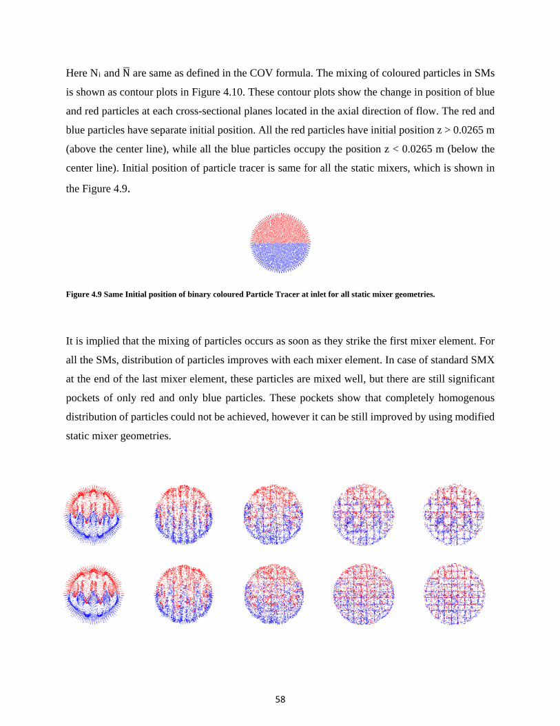
58
Here Ni and N� are same as defined in the COV formula. The mixing of coloured particles in SMs
is shown as contour plots in Figure 4.10. These contour plots show the change in position of blue
and red particles at each cross-sectional planes located in the axial direction of flow. The red and
blue particles have separate initial position. All the red particles have initial position z > 0.0265 m
(above the center line), while all the blue particles occupy the position z < 0.0265 m (below the
center line). Initial position of particle tracer is same for all the static mixers, which is shown in
the Figure 4.9.
Figure 4.9 Same Initial position of binary coloured Particle Tracer at inlet for all static mixer geometries.
It is implied that the mixing of particles occurs as soon as they strike the first mixer element. For
all the SMs, distribution of particles improves with each mixer element. In case of standard SMX
at the end of the last mixer element, these particles are mixed well, but there are still significant
pockets of only red and only blue particles. These pockets show that completely homogenous
distribution of particles could not be achieved, however it can be still improved by using modified
static mixer geometries.

59
(a) (b) (c) (d) (e)

60
Figure 4.10 Comparison of distribution of binary coloured Particle Tracer contour plots for all static mixer geometries at Re = 30.
(a) After 1st mixer element (b) After 2nd mixer element (c) After 4th mixer element (d) After 6th mixer element (e) After last mixer element. From top to bottom each row represents the contour plots for the following geometries: SMX, Perforated SMX, Perforated SMX 4 holes, Perforated SMX maximum no. of D/20 holes, Perforated SMX maximum no. of D/30 holes, Perforated SMX maximum no. of D/40 holes, SMX with circular serrations, SMX with triangular serrations and SMX with square serrations.
It is apparent that perforated SMX of D/30 gives the best distributive mixing of blue and red
particles among all the static mixers. Perforated SMX of D/20 also gives very good distributive
mixing pattern, however it does not seem to be as good as D/30 perforations. All three serrated
SMX geometries show less distributive mixing capabilities than the D/20 or D/30 perforations but
it is still much better than the standard SMX. Distributive mixing capacity of static mixers cannot
be judged based on the visual contour plots only. It is essential to analyze it based on the data of
standard deviation too. Figure 4.11 shows the plot of change in standard deviation with the
increasing mixer elements for Reynolds number 30. The data in Figure 4.11 shows that after 8
mixer elements, standard deviation value reduces to almost 54% for SMX. If initial position of
red/blue particles (above and below the center line respectively) is considered to be 100% deviation
then, ideally lower the value of standard deviation, higher the distributive mixing would be. Ideally
0% deviation represents uniform distribution of red/blue particles across the cross-sectional plane.
Figure 4.11: Comparison of Standard Deviation vs Number of mixing elements plot for all the static mixer geometries at Re = 30.

61
Distributive mixing capacity of SMX static mixer is definitely enhanced by incorporating the
perforations on the blades. However, decreasing the size of perforations below the D/30, the
distributive mixing capacity is deteriorated. Circular and triangular serrated SMX demonstrate
enhanced particle distribution and lower standard deviation values of 24% and 27% respectively.
However, it is still not as good as D/30 and D/20 perforations which gave standard deviation values
of 16% and 21% respectively. It is observed that square serrated SMX might not be good in terms
of dispersive mixing but it is better than SMX mixer when it comes to distributive mixing. Based
on the comparison of standard deviation values it is implied that in terms of distributive mixing
D/30 Perforated SMX > D/20 Perforated SMX > Circular serrated SMX > triangular serrated
SMX. As the Reynolds number increases, the distributive mixing also increases with increasing
velocity and inertial effects of the fluid. It must be noted that the lowest deviation value achieved
was 16% in case of Reynolds number equals to 30. This value would be different if different grid
size is placed on cross-sectional plane for each case, but it would not change the trend observed
with respect to the standard deviation.
4.4 Final Comparison
The performance of all the static mixers have been characterized in terms of dispersive mixing and
distributive mixing. The final comparison of all the static mixers is shown in the Table 4.2. It is
clear that circular serrated SMX impose minimum shear rate. It means that minimum energy is
lost in generating shear and it results into lowest pressure drop among all the SMs. Circular serrated
SMX has highest extensional efficiency among all the static mixers, demonstrating highest
dispersion capacity and elongational flow. Triangular serrations gives slightly higher pressure drop
and has less extensional efficiency than the circular serrated SMX. A similar trend is observed for
D/20 perforated SMX, with a poor performance than the triangular SMX. However, in terms of
distributive mixing, D/20 perforated SMX is better than circular and triangular SMX. D/30
Perforated SMX gives highest distributive mixing, but it gives poor dispersive mixing.

62
Table 4.2 Final Comparison of static mixers
Type of static mixer
Dispersive Mixing Distributive mixing
Pressure Drop (∆P)
(Pa)
Mean velocity
(m/s)
Mean Shear rate (1/s)
Extensional Efficiency
Standard Deviation at the end of
8th element (%)
SMX 0.1185 0.0006 0.2541 0.5647 54.8266 Perf SMX 0.1128 0.00059 0.2481 0.5695 41.4651
Perf SMX 4 holes 0.1101 0.00059 0.2470 0.5719 28.9088 D/20 Perforated SMX 0.0905 0.00058 0.2456 0.5714 21.5160 D/30 Perforated SMX 0.1117 0.0006 0.2481 0.5744 16.2521 D/40 Perforated SMX 0.1197 0.00058 0.2518 0.5643 50.3718
Circular 0.0787 0.00056 0.2203 0.5734 23.9109 Triangular 0.0815 0.00058 0.2237 0.5649 27.3613
Square 0.1070 0.00059 0.2496 0.5705 30.7914
From the comparison of different parameters shown in Table 4.2, it is clear that the choice of mixer
should be such that it shows good mixing in terms of both dispersive and distributive. Circular
SMX may not give good distributive mixing, but it is still better than the standard SMX mixer. By
taking into considerations all of these factors, it can be concluded that circular serrated SMX gives
better performance than standard SMX mixer and it would be the best choice among all static
mixers compared in this work. Another implication would be that the triangular serrated SMX and
D/20 perforated SMX also give much better performance than SMX. Triangular serrated SMX
gives higher dispersion, while D/20 perforated SMX gives higher distributive mixing.

63
CHAPTER 5: Application of Static Mixer in Polymerization
5.1 Introduction
Static mixers have a wide range of industrial applications and are predominantly used in polymer
industry. First commercial application of static mixers at pilot scale was reported in 1984, for the
production of polystyrene [56]. Ever since, the use of static mixers in polymer industry has
increased significantly. Other applications of SMs in polymer industry includes blending of
polymers, synthesis of in-situ nanocomposites and nanoparticles, polymer extrusion process,
emulsification processes and in the production of many commodity polymers.
The choice of reactor in the synthesis of polymer depends on the reaction kinetics and viscosity of
the polymer. Continuous stirred tank reactor (CSTR) is generally used for the homogenous
polymerization reaction with high termination rate, as it gives narrowest molecular weight
distribution and higher conversion. On the other hand, tubular reactor can be used for the
continuous bulk polymerization of commodity polymers due to its simplicity and low cost of
operation as there are no moving parts. However due to high viscosity of reaction mixture, poor
radial mixing is achieved which is a major drawback of using a tubular reactor for polymerization.
This in turn results into higher conversion of monomer near the walls where velocities are very
low and lower conversions at the center where velocity is maximum. This problem can be
overcome by using static mixers in polymerization process. Since static mixers provide higher
axial and radial mixing, similar to plug flow behavior is achieved resulting into narrower molecular
weight distribution of polymer. An additional benefit would be, continuous production of polymers
can be achieved by incorporating static mixers.
Use of static mixers in the industrial production of polymers has increased tremendously. Amidst
all, the synthesis of polyacrylamide has gained significant interest due to its application in
enhanced oil recovery (EOR). In this process, static mixers are used to mix partially hydrolyzed
polyacrylamide (HPAM) with injected water to recover the oil from reservoir. Since this polymer
solution is extremely viscous, static mixers are used to perform this operation. SMs are
commercially proven best device to carry out this type of operations in EOR process. Though
polyacrylamide is used to a large extent in EOR, maximum consumption of polyacrylamide is in
64
the process of flocculating solids in a liquid. Largest use of polyacrylamide is in water treatment,
paper making and screen printing. With the improving technology, synthesis of PAM process has
started incorporating the use of static mixers in production process. However, it is restricted to lab
scale only.
This chapter facilitates preliminary CFD model for the synthesis of polyacrylamide using static
mixers. Given the fact that actual homopolymerization of acrylamide involves several reactions,
this CFD model has included only major reactions such as initiation, propagation and termination.
In the current work, synthesis of polyacrylamide was performed using the SMX static mixer and
its performance is compared to that of the circular serrated SMX geometry, which is the best
among all the modified static mixer geometries. The performance of both static mixers has been
analyzed based on the final polymer concentration, reaction rate and monomer conversion.
Comparison of results are shown in terms of contour plots and line plots. In the next part,
description about the materials and method of polymerization used for CFD model for acrylamide
polymerization is given.
5.2 CFD model for homopolymerization of acrylamide
Acrylamide monomer undergoes polymerization by redox initiation. Polymerization can also be
induced by photo initiation, radiation, electron initiation and by ultrasonic waves [57]. However,
the principal method of industrial production of PAM and its derivatives is either free-radical
homopolymerization in solution or emulsion polymerization [58]. This model gives an insight of
actual homopolymerization experiment in case of two different static mixer geometries.
5.2.1 Materials and Reaction Mechanism
In this study, polymerization of acrylamide is initiated by activating the monomer by Potassium
Persulfate initiator. The concentration of initiator was 5.21x10⁻² moles/liter, while the monomer
concentration was 0.04 moles/liter. For all simulations, isothermal conditions have been adopted
and polymerization temperature is assumed to be constant at 30° C. For this CFD model, all initial
conditions and input parameters for both static mixer geometries have been shown in Table 5.1.
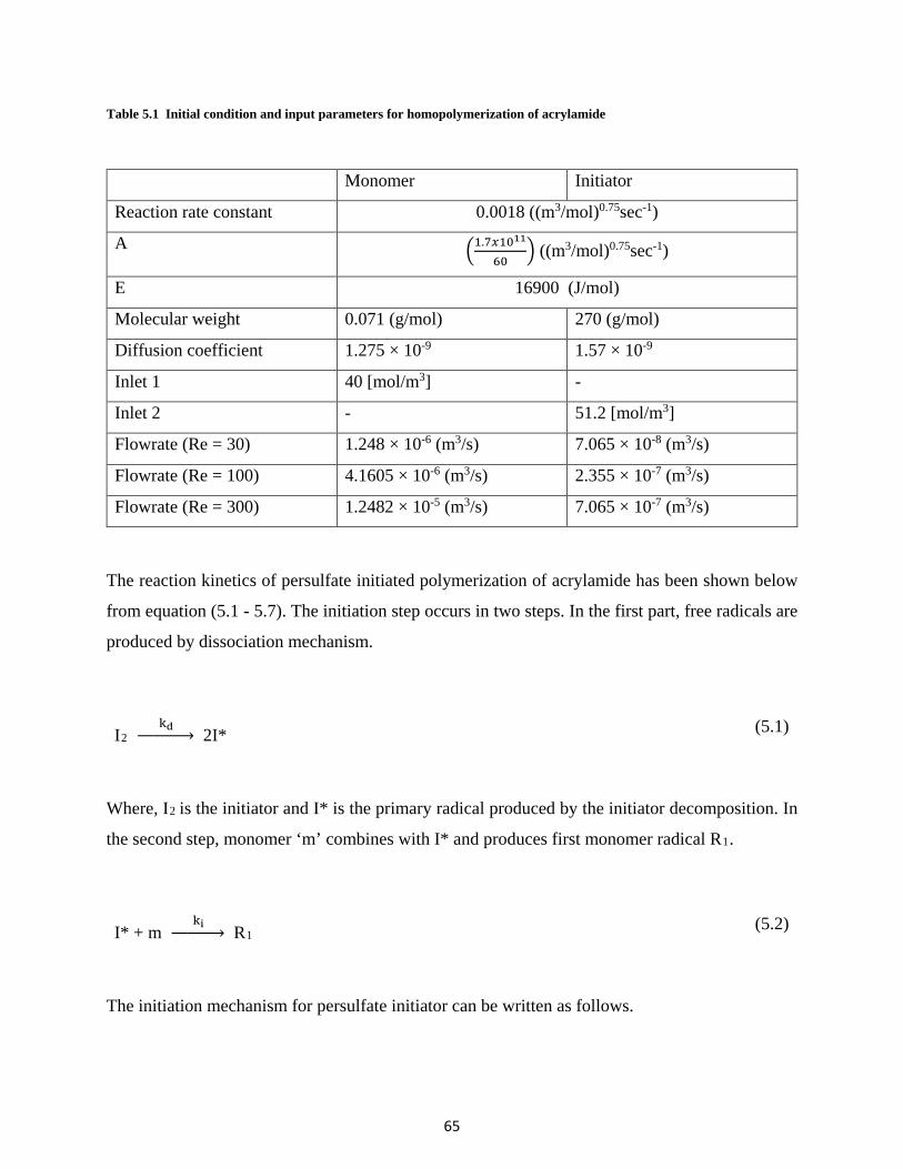
65
Table 5.1 Initial condition and input parameters for homopolymerization of acrylamide
Monomer Initiator
Reaction rate constant 0.0018 ((m3/mol)0.75sec-1)
A �1.7𝑥𝑥1011
60� ((m3/mol)0.75sec-1)
E 16900 (J/mol)
Molecular weight 0.071 (g/mol) 270 (g/mol)
Diffusion coefficient 1.275 × 10⁻⁹ 1.57 × 10⁻⁹
Inlet 1 40 [mol/m3] -
Inlet 2 - 51.2 [mol/m3]
Flowrate (Re = 30) 1.248 × 10⁻⁶ (m3/s) 7.065 × 10⁻⁸ (m3/s)
Flowrate (Re = 100) 4.1605 × 10⁻⁶ (m3/s) 2.355 × 10⁻⁷ (m3/s)
Flowrate (Re = 300) 1.2482 × 10⁻⁵ (m3/s) 7.065 × 10⁻⁷ (m3/s)
The reaction kinetics of persulfate initiated polymerization of acrylamide has been shown below
from equation (5.1 - 5.7). The initiation step occurs in two steps. In the first part, free radicals are
produced by dissociation mechanism.
I2 kd �⎯⎯⎯⎯⎯� 2I* (5.1)
Where, I2 is the initiator and I* is the primary radical produced by the initiator decomposition. In
the second step, monomer ‘m’ combines with I* and produces first monomer radical R1.
I* + m ki �⎯⎯⎯⎯⎯� R1 (5.2)
The initiation mechanism for persulfate initiator can be written as follows.
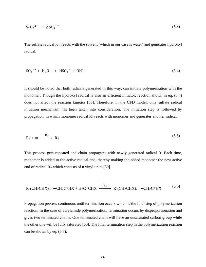
66
S2O82− → 2 SO4
−∗ (5.3)
The sulfate radical ion reacts with the solvent (which in our case is water) and generates hydroxyl
radical.
SO4−∗ + H2O → HSO4
− + OH∗ (5.4)
It should be noted that both radicals generated in this way, can initiate polymerization with the
monomer. Though the hydroxyl radical is also an efficient initiator, reaction shown in eq. (5.4)
does not affect the reaction kinetics [55]. Therefore, in the CFD model, only sulfate radical
initiation mechanism has been taken into consideration. The initiation step is followed by
propagation, in which monomer radical R1 reacts with monomer and generates another radical.
R1 + m kp �⎯⎯⎯⎯⎯� R2 (5.5)
This process gets repeated and chain propagates with newly generated radical R. Each time,
monomer is added to the active radical end, thereby making the added monomer the new active
end of radical Rn which consists of n vinyl units [59].
R-(CH2CHX)n-1 ─CH2C*HX + H2C=CHX kp �⎯⎯⎯⎯⎯� R-(CH2CHX)n-1 ─CH2C*HX (5.6)
Propagation process continuous until termination occurs which is the final step of polymerization
reaction. In the case of acrylamide polymerization, termination occurs by disproportionation and
gives two terminated chains. One terminated chain will have an unsaturated carbon group while
the other one will be fully saturated [60]. The final termination step in the polymerization reaction
can be shown by eq. (5.7).
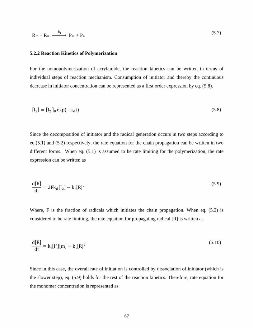
67
Rm + Rn kt �⎯⎯⎯⎯� Pm + Pn (5.7)
5.2.2 Reaction Kinetics of Polymerization
For the homopolymerization of acrylamide, the reaction kinetics can be written in terms of
individual steps of reaction mechanism. Consumption of initiator and thereby the continuous
decrease in initiator concentration can be represented as a first order expression by eq. (5.8).
[I2] = [I2 ]0 exp(−kdt) (5.8)
Since the decomposition of initiator and the radical generation occurs in two steps according to
eq.(5.1) and (5.2) respectively, the rate equation for the chain propagation can be written in two
different forms. When eq. (5.1) is assumed to be rate limiting for the polymerization, the rate
expression can be written as
d[R]dt
= 2Fkd[I2] − kt[R]2 (5.9)
Where, F is the fraction of radicals which initiates the chain propagation. When eq. (5.2) is
considered to be rate limiting, the rate equation for propagating radical [R] is written as
d[R]dt
= ki[I∗][m] − kt[R]2 (5.10)
Since in this case, the overall rate of initiation is controlled by dissociation of initiator (which is
the slower step), eq. (5.9) holds for the rest of the reaction kinetics. Therefore, rate equation for
the monomer concentration is represented as

68
d[m]dt
= −2Fkd[I2] − kp[R][m] (5.11)
It necessary to consider only those initiator radicals which add the monomer and activates the
chain propagation. Some initiating radicals recombine with other radicals or they decompose into
non-initiating radicals. For this reason, only very small fraction ‘F’ of initiator concentration
contributes to chain polymerization and thereby, the rate equation of monomer concentration can
be written as
d[m]dt
= −kp[R][m] (5.12)
In the overall polymerization reaction, radicals are generated in the initiation step and get
consumed in the termination step. This condition leads to quasi steady state condition, which can
be expressed as
d[I∗]dt
=d[R]
dt ~ 0
(5.13)
By substituting the eq.(5.13) in eq.(5.9), the radical concentration can be expressed as
R = �2Fkd[I2]
kt
(5.14)
Finally, substituting eq. (5.14) in (5.12), the overall rate equation for monomer consumption is
written as
d[m]dt
= −kp�2Fkd[I2]
kt [m]
(5.15)

69
The eq. (5.15) shows the overall rate of free radical polymerization is proportional to monomer
concentration and to the square root of initiator concentration.
Once the reaction rate expression is determined in terms of monomer and initiator concentration,
values of reaction rate parameters are included in the CFD model. For the reaction rate shown in
eq. (5.15), the value of overall reaction rate constant k at 30°C is
k = kp�2Fkdkt
= 0 .108 + 0.003 liter0.75
mole0.75min
(5.16)
In the CFD model, the kinetics parameters can also be expressed as Arrhenius expression [61].
Which is
k = 1.70 × 10¹¹exp �−16900RT
� liter0.75
mole0.75min (5.17)
In the current CFD model, polymerization reactions taking place inside the SMX and circulated
SMX geometries are coupled with the reaction kinetics and flow conditions of reactants and
resulting polymer. For all the simulations, laminar flow conditions of monomer and initiator fluid
streams are used. As Polyacrylamide is non-Newtonian fluid, the viscosity of polymer increases
with the increasing molecular weight. The viscosity expression for the generation of
polyacrylamide solution is given by eq. (5.18) [61].
µ = 6.8 × 10⁻⁴ (Mn)0.66 (5.18)
It must be mentioned that, in actual lab experiments the viscosity is measured by means of Huggins
equation
µspc
= (µ) + k′(µ)2c (5.19)
Where µsp is the pure solvent viscosity, k’ is the Huggins constant and c is the solution
concentration. Since the similar process conditions as mentioned by John Perry [61] are used to
simulate the CFD model here, the simpler expression of viscosity variation (eq. (5.18)) is utilized.
Apart from reaction mechanism and reaction kinetics it is necessary to understand basic equation
which governs the flow simulations for this computational model. In addition to the eq. (3.9), this

70
computational model uses the eq.(5.20) which represents diffusion of reactants and implements
the mass balance [52].
∂c∂t
+ u.∇c = ∇. (𝐷𝐷∇c) + 𝑅𝑅 (5.20)
Where, c is the concentration of the species (SI unit: mol/m3), D represents the diffusion co-
efficient (SI unit: m2/s), R denotes reaction rate expression for the species (SI unit: (mol) / (m3.s))
and u is the velocity of species (SI unit: m/s).
The first term on left hand side in eq. (5.20) accounts for the consumption of the species. In this
case, it is represented by eq.(5.9) and (5.12) for the consumption of initiator and monomer
respectively. The second term shown in eq. (5.21) corresponds to convective transport of species
due to a velocity field ‘u’. Since in this case, laminar flow interface is coupled with this
computational model, velocity field works as model input and it is computed from the momentum
balance shown by (3.9) in Chapter 3.
The first term on the right hand side of eq. (5.20) denotes the diffusive transport which accounts
for the interaction between monomer and initiator involved in the reaction. The values used for
diffusion coefficient of monomer and initiator are shown in Table 5.1 [62,63]. Value of diffusion
coefficient depends on the type of solute/solvent system and temperature. Earlier literature data
gives experimentally measured values of diffusion coefficient of acrylamide in case of components
such as KCL and D2O [63]. These values are apparently in the same range of reported values of
diffusion coefficient of acrylamide in water, which is 1.275 × 10⁻⁹ [64]. Due to lack of knowledge
in the literature data for an exact value of diffusion coefficient of acrylamide monomer with
potassium persulfate initiator, it is suggested to use above mentioned value of D for acrylamide
monomer.
The second term on the right hand side of eq. (5.20) illustrates various chemical reactions involved.
In case of homopolymerization of acrylamide, for the simplicity of model, reaction involving both
acrylamide monomer and potassium persulfate initiator is used to achieve final polyacrylamide
product. In the next section, the results of numerical simulations for the polyacrylamide are shown
in the form of polymer concentration, reaction rate monomer conversion.

71
5.3 Results of homopolymerization of acrylamide model
CFD model for homopolymerization of acrylamide has been solved for two cases: 1) SMX static
mixer and 2) Circular serrated SMX geometry. Since the circular serrated SMX geometry gives
the best performance among all modified static mixer geometries, it has been selected for
homopolymerization of acrylamide. Though same dimensions of the static mixer geometries of are
used for the polymerization, it must be mentioned that an additional inlet for the injection of
initiator has been provided in both the cases. In Figure 5.1 and Figure 5.2, static mixer geometries
used in the simulations are shown. The purpose of providing an additional inlet port (inlet 2) is to
inject the initiator stream inside the reactor, whereas monomer is injected from the main pipe inlet
only.
Figure 5.1 SMX static mixer geometry 8 elements with additional pipe inlet for the initiator inflow
Figure 5.2 Circulated SMX serrated static mixer geometry 8 elements with additional pipe inlet for the initiator flow
The results for the chemical reaction along with the flow field calculations are shown from Figure
5.3 to Figure 5.5 for SMX and Circular serrations. These figures show the streamlines of the flow
field for a Reynolds number 30 for both geometries. The colour expression represents the
concentration change in the polymer product. Colour scale from blue to red represents the
minimum to maximum concentration of the resulting polymer.

72
(a) (b)
Figure 5.3 Comparison of Concentration of resulting polyacrylamide for (a) SMX geometry (b) Circular serrated SMX geometry
From the streamlines plots shown in Figure 5.3 to Figure 5.5, the mixing effects are evident in the
region where second inlet port for initiator is provided. In both the cases, the polymerization
reaction starts as soon as the initiator comes into contact with the monomer. From Figure 5.3, it is
apparent that due to the higher mixing ability of circular serrations, the polymerization reaction
starts early and attains higher polymer concentration values than the SMX geometry. Further,
Figure 5.4 and Figure 5.5 shows the streamline plots for both the geometries in the form of initiator
concentration and monomer concentration respectively.
(a) (b)
Figure 5.4 Comparison of Concentration of initiator for (a) SMX geometry (b) Circular serrated SMX geometry

73
(a) (b)
Figure 5.5 Comparison of Concentration of monomer for (a) SMX geometry (b) Circular serrated SMX geometry
During the polymerization, the reactant monomer and initiator are consumed along the length of
the reactor. The injection stream of second inlet port of initiator mixes with the main monomer
stream and results into non-uniform distribution of initiator in the SMX geometry (shown as the
blue stream in Figure 5.4 (a), which is longer). Depending on the degree of mixing of initiator and
monomer, the rate of generation of polymer varies. Figure 5.5 (a) shows that SMX geometry has
relatively higher monomer concentration in the flow domain, which implies relatively less
monomer is converted during the polymerization.
Mixing is more effective in the circular serrations, therefore initiator distribution is relatively more
uniform (shown as the blue stream of initiator in Figure 5.4 (b) which is shorter). In case of circular
serrated SMX geometry relatively lower monomer concentration is observed, which indicates
more consumption of monomer in producing higher concentration of polymer. The purpose of
comparing the streamline plots was to demonstrate the reaction kinetics coupled with the flow field
of injected reactant streams. However, they are not sufficient to show that the circular serrated
SMX improves the homopolymerization of acrylamide.
In order to analyze the actual static mixer performance for polymerization system, comparison is
shown in terms of reaction rate and monomer conversion for both the reactors. Figure 5.6 and
Figure 5.7 shows line plots for the variation of reaction rate along the axial length of the reactor
for SMX and circular serrations respectively.
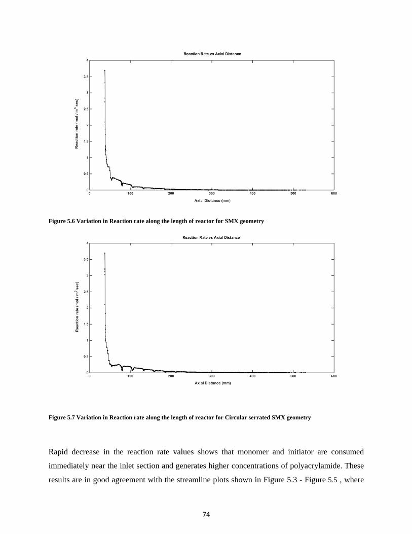
74
Figure 5.6 Variation in Reaction rate along the length of reactor for SMX geometry
Figure 5.7 Variation in Reaction rate along the length of reactor for Circular serrated SMX geometry
Rapid decrease in the reaction rate values shows that monomer and initiator are consumed
immediately near the inlet section and generates higher concentrations of polyacrylamide. These
results are in good agreement with the streamline plots shown in Figure 5.3 - Figure 5.5 , where

75
higher concentration gradients of monomer and initiator are present in the inlet region and
indicates higher consumption of reactants. It should be noted that since initiator is injected from
the second inlet, there is no reaction occurring in that region. Due to this, polymer generation starts
after the second inlet port when initiator starts mixing with the monomer.
Rapid changes in reaction rate plots indicates the movement of fluid streams through the static
mixers. As the fluid stream of initiator and monomer moves forward through the mixer elements,
it gets split, rotated and mixed. This type of fluid stream movement results into sudden reaction
rate gradients. Figure 5.7 shows higher reaction rate gradients as compared to that of shown in
Figure 5.6, which also implies better mixing of monomer and initiator in circular serrated SMX
than standard SMX geometry. Higher the mixing, higher is the contact between monomer and
initiator which gives more polymer yield. Concentration of monomer and initiator decreases along
the length of the reactor, which reduces the rate of polymerization shown by eq. (5.15). Zero
reaction rate indicates that monomer is completely converted into polymer. Therefore it is desired
to achieve reaction rate values approaching zero. All the plots of reaction rates are directly
correlated to the plots of monomer conversion, which is shown by eq. (5.21).
Conversion = 1 − � M M0� (5.21)
Where M is the monomer conversion at any point in the reactor and M0 is the initial monomer
concentration. Figure 5.8 and Figure 5.9 shows the plots of monomer conversion for SMX and
circular SMX geometry.
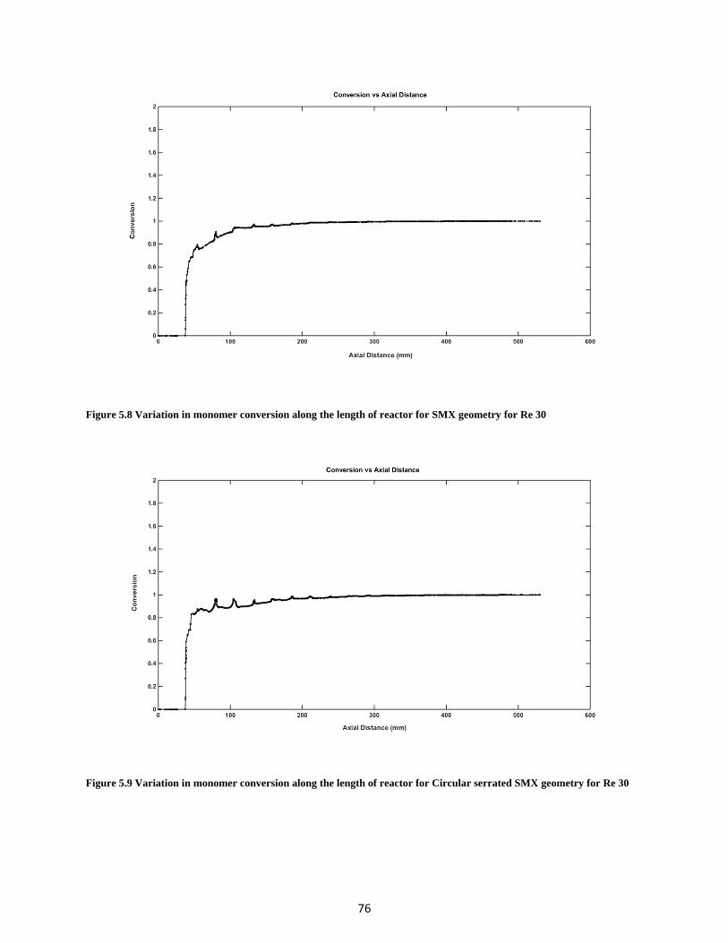
76
Figure 5.8 Variation in monomer conversion along the length of reactor for SMX geometry for Re 30
Figure 5.9 Variation in monomer conversion along the length of reactor for Circular serrated SMX geometry for Re 30
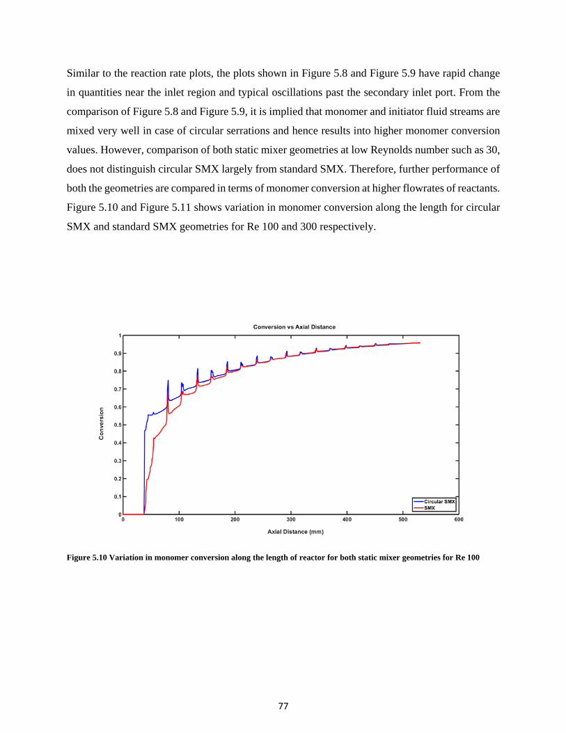
77
Similar to the reaction rate plots, the plots shown in Figure 5.8 and Figure 5.9 have rapid change
in quantities near the inlet region and typical oscillations past the secondary inlet port. From the
comparison of Figure 5.8 and Figure 5.9, it is implied that monomer and initiator fluid streams are
mixed very well in case of circular serrations and hence results into higher monomer conversion
values. However, comparison of both static mixer geometries at low Reynolds number such as 30,
does not distinguish circular SMX largely from standard SMX. Therefore, further performance of
both the geometries are compared in terms of monomer conversion at higher flowrates of reactants.
Figure 5.10 and Figure 5.11 shows variation in monomer conversion along the length for circular
SMX and standard SMX geometries for Re 100 and 300 respectively.
Figure 5.10 Variation in monomer conversion along the length of reactor for both static mixer geometries for Re 100
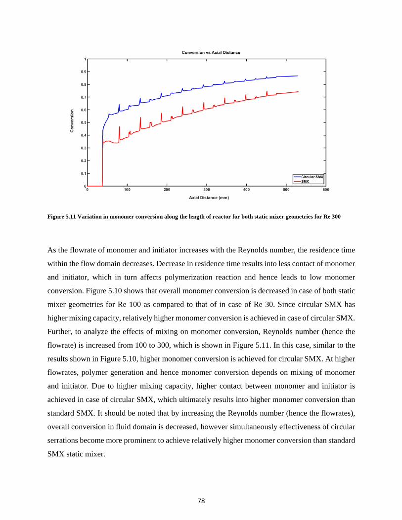
78
Figure 5.11 Variation in monomer conversion along the length of reactor for both static mixer geometries for Re 300
As the flowrate of monomer and initiator increases with the Reynolds number, the residence time
within the flow domain decreases. Decrease in residence time results into less contact of monomer
and initiator, which in turn affects polymerization reaction and hence leads to low monomer
conversion. Figure 5.10 shows that overall monomer conversion is decreased in case of both static
mixer geometries for Re 100 as compared to that of in case of Re 30. Since circular SMX has
higher mixing capacity, relatively higher monomer conversion is achieved in case of circular SMX.
Further, to analyze the effects of mixing on monomer conversion, Reynolds number (hence the
flowrate) is increased from 100 to 300, which is shown in Figure 5.11. In this case, similar to the
results shown in Figure 5.10, higher monomer conversion is achieved for circular SMX. At higher
flowrates, polymer generation and hence monomer conversion depends on mixing of monomer
and initiator. Due to higher mixing capacity, higher contact between monomer and initiator is
achieved in case of circular SMX, which ultimately results into higher monomer conversion than
standard SMX. It should be noted that by increasing the Reynolds number (hence the flowrates),
overall conversion in fluid domain is decreased, however simultaneously effectiveness of circular
serrations become more prominent to achieve relatively higher monomer conversion than standard
SMX static mixer.
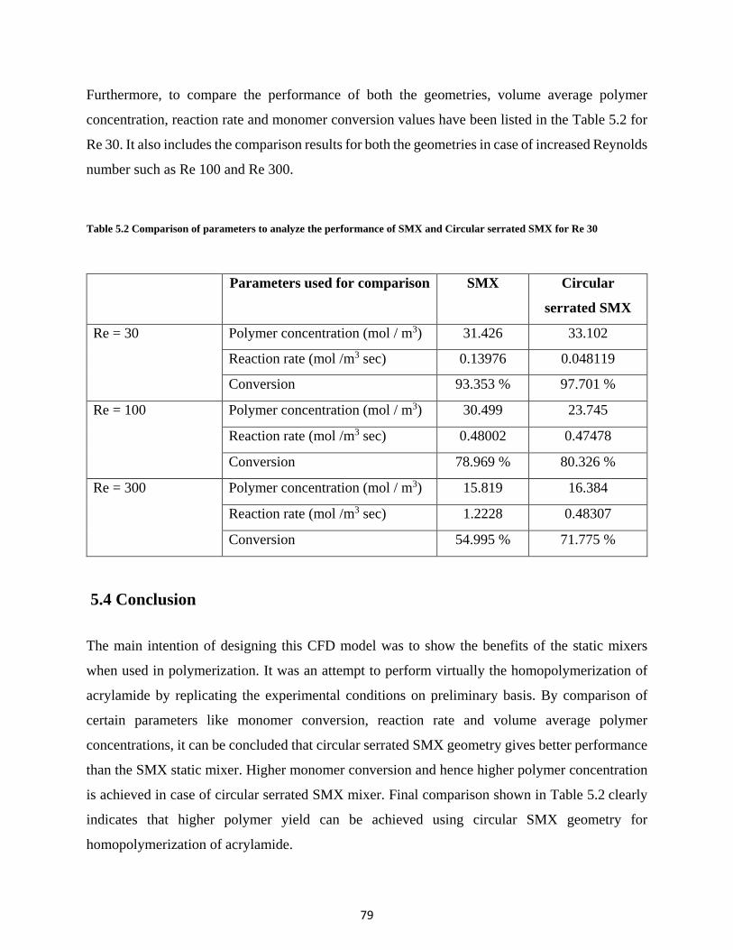
79
Furthermore, to compare the performance of both the geometries, volume average polymer
concentration, reaction rate and monomer conversion values have been listed in the Table 5.2 for
Re 30. It also includes the comparison results for both the geometries in case of increased Reynolds
number such as Re 100 and Re 300.
Table 5.2 Comparison of parameters to analyze the performance of SMX and Circular serrated SMX for Re 30
Parameters used for comparison SMX Circular
serrated SMX
Re = 30 Polymer concentration (mol / m3) 31.426 33.102
Reaction rate (mol /m3 sec) 0.13976 0.048119
Conversion 93.353 % 97.701 %
Re = 100 Polymer concentration (mol / m3) 30.499 23.745
Reaction rate (mol /m3 sec) 0.48002 0.47478
Conversion 78.969 % 80.326 %
Re = 300 Polymer concentration (mol / m3) 15.819 16.384
Reaction rate (mol /m3 sec) 1.2228 0.48307
Conversion 54.995 % 71.775 %
5.4 Conclusion
The main intention of designing this CFD model was to show the benefits of the static mixers
when used in polymerization. It was an attempt to perform virtually the homopolymerization of
acrylamide by replicating the experimental conditions on preliminary basis. By comparison of
certain parameters like monomer conversion, reaction rate and volume average polymer
concentrations, it can be concluded that circular serrated SMX geometry gives better performance
than the SMX static mixer. Higher monomer conversion and hence higher polymer concentration
is achieved in case of circular serrated SMX mixer. Final comparison shown in Table 5.2 clearly
indicates that higher polymer yield can be achieved using circular SMX geometry for
homopolymerization of acrylamide.
80
CHAPTER 6: Conclusions
6.1 Concluding Remarks
The objective of this research was to improve the mixing performance of static mixer by
incorporating design modifications to it. For that purpose, computational simulations were
performed using COMSOL Multiphysics and numerical results of the modified SMX geometries
were compared with SMX mixer. Flow field calculations and pressure drop results obtained for
SMX geometry were in good agreement with the published literature values [54], which validates
the reliability of CFD model. Besides the pressure drop, four criterion were chosen to compare the
mixing performance of static mixer: mean velocity, mean shear rate, extensional efficiency and
variation in the standard deviation.
It was found that SMX with circular serrations reduces the pressure drop approximately by 33-
35% than that of the standard SMX mixer, which makes it most energy efficient mixer among all
the static mixer geometries. Moreover, from the comparison of dispersive mixing parameters
shown in Table 4.2, it appeared that circular serrated SMX had maximum extensional efficiency,
causing higher dispersion and elongational flows than other mixer geometries. It should be noted
that both triangular serrations and D20 perforated SMX reduced the pressure drop significantly
and showed excellent dispersive mixing than the standard SMX mixer, but it was not as good as
the circular serrated SMX geometry. However, when it came to distributive mixing, D/20
perforated SMX gave better results than circular serrated SMX. Since perforations on each blade
gives an extra passage to the particles flowing through SMs, particle distribution is much better in
the case of D/20 perforated SMX than the circular serrations. Further, it is observed that D/30
perforated SMX showed maximum distributive mixing, but it had poor dispersive mixing. From
the comparison of dispersive and distributive mixing parameters, it is clear that as the size of
perforations is decreased overall mixing performance gets deteriorated.
In practical applications, performance of static mixer is analyzed based on both the dispersive
mixing and distributive mixing. Given the fact that circular serrated SMX could not facilitate the
best distributive mixing, it was still far better than the standard SMX mixer (reducing standard

81
deviation by 30%). By considering all the factors, it can be concluded that circular serrated SMX
is much better than SMX mixer and it would be the most efficient among all the modified static
mixer geometries used in this study. Another implication would be that the triangular serrated
SMX and D/20 perforated SMX are rather similar and give better mixing than SMX. For D/30
SMX the distributive mixing was improved significantly but pressure drop was too high with
marginal improvement in dispersive mixing. In case of square serrated SMX, though overall better
mixing was achieved, it was not better mixer as compared to circular serrated SMX. Further, it
was observed that by decreasing the holes size from D/30 to D/40, the overall mixing performance
deteriorated and resulted into higher pressure drop than the standard SMX mixer.
In Chapter 5 as a part of static mixer applications, circular serrated SMX was used to simulate
homopolymerization of acrylamide. Since circular serrated SMX improves the mixing
significantly, for the same process conditions higher monomer conversion was achieved. Due to
improved mixing of monomer and initiator, higher concentration of polymer was achieved in the
SM reactor with circular serrations. In this work, only virtual homopolymerization is performed
through CFD model, but it gives an insight of potential improvement in polyacrylamide production
process depending on the experimental validity.
6.2 Recommendations
Further, experimental investigation should be carried out using the SMX and circular serrated
SMX mixer and by changing the working fluid from water to glycerin. Due to limited options
available in COMSOL, there are constraints on movement of particles and hence on the
transmission probability of particles through the mixer. Due to which, not all the particles come
out of the reactor pipe and some of them get stuck on the mixer wall. These limitations can be
overcome by carrying out the actual experiments with glycerin fluid and particle tracer. Since in
reality minor loss of particle tracer occurs, results can be verified for Re 1, 30 & 100 with published
literature data [40]. This one could be a potential way to check the repeatability of distributive
mixing analysis.
For the polymerization of acrylamide, the CFD model is just an attempt to get an insight of
potential benefits of using circular serrated SMX over standard SMX mixer. In actual experiment
82
of synthesis of polyacrylamide involves numerous reactions, however the scope of reactions in the
CFD model is restricted to the main reaction mechanism only. Moreover, in reality produced
polyacrylamide also depends on some pre-requisites steps, nature of initiator, pH of solvent and
temperature etc. Though CFD model has included as many things as possible, it cannot replicate
the actual experimental procedure in simulations. Therefore it is recommended to carry out an
actual homopolymerization experiment to generate the PAM using circular serrated SMX. Since
hydrolyzed polyacrylamide (HPAM) is mainly used in EOR process, this work may inspire to
extend it further and perform synthesis of HPAM using the circular serrated SMX mixer.

83
References
[1] J. Gyenis, “Motionless mixer in bulk solids treatment- A review,” Kona , vol. 20, no. 20, pp. 9–23, 2002.
[2] A. Ghanem, T. Lemenand, D. Della Valle, and H. Peerhossaini, “Static mixers: Mechanisms, applications, and characterization methods - A review,” Chem. Eng. Res. Des., vol. 92, no. 2, pp. 205–228, 2014.
[3] Chemineer Inc., “Kenics Static Mixing Technology,” Manual, p. 12, 2013.
[4] Y. D. K. Gmbh, “Static mixer for mobile materials having horizontal cylinder with cooling jacket filled with packing such as spheres with vibrator attached,” Pat. DE2815651A1, p. 2815651, 1978.
[5] B. and LOBBE, “PENTAX and N-Form,” Catalogue, TECHNOLOGY, SPX FLOW. .
[6] T. Engineering, “Mixing Nozzle for Injection Molding Machines.”
[7] F. Petzholdt, “PSM-4, STATIC MIXER.” pp. 1–5, 2016.
[8] K. S. Inc., “Triple Action Static Mixer.” .
[9] S. Mixers, P. Mixers, and P. S. Gmbh, “‘Pulsating Mixing Reactor’ (PMR) static mixer.” pp. 1–2, 2015.
[10] T. F. Cootes, C. Twining, I. Limited, and P. E. L. Rodriguez, “United States Patent,” vol. 2, no. 12, 2009.
[11] M. Gavrilescu and R. Z. Tudose, “Intensification of transfer processes in biotechnology and chemical engineering using static mixers.(Review),” Acta Biotechnol., vol. 15, pp. 3–26, 2004.
[12] R. Thakur, C. Vial, and K. Nigam, “Static mixers in the process industries—a review,” … Res. Des., vol. 81, no. 7, pp. 787–826, 2003.
[13] E. L. Paul, V. a Atiemo-obeng, and S. M. Kresta, HANDBOOK OF INDUSTRIAL MIXING Edited by. 2004.
[14] a. Jaya, “Static Mixer (Engineering Design Guideline),” KLM Technol. Gr., pp. 1–47, 2014.
[15] H. Abbasfard, M. Ghanbari, A. Ghasemi, G. Ghahraman, S. M. Jokar, and M. R. Rahimpour, “CFD modelling of flow mal-distribution in an industrial ammonia oxidation reactor: A case study,” Appl. Therm. Eng., vol. 67, no. 1–2, pp. 223–229, 2014.

84
[16] P. J. Roache, “Computational Fluid Dynamics.” Hermosa, New Mexico., 1976.
[17] S. N. Shintre and J. J. Ulbrecht, “a Model of Mixing in a Motionless Mixer,” Chem. Eng. Commun., vol. 24, no. 1–3, pp. 115–138, 1983.
[18] J. Arimond and L. Erwin, “a Simulation of a Motionless Mixer,” Chem. Eng. Commun., vol. 37, no. 1–6, pp. 105–126, 1985.
[19] J. M. Ottino, “The Kinematics of Mixing Stretching, Chaos, and Transport.” 1989.
[20] K. D. & E. B. NAUMAN, “Fully Developed Flow in Twisted Tapes : a Model for Motionless Mixers Fully Developed Flow in Twisted Tapes : a Model for Motionless Mixers,” vol. 6445, no. April 2013, pp. 37–41, 2007.
[21] F. H. Ling and X. Zhang, “a Numerical Study on Mixing in the Kenics Static Mixer,” Chem. Eng. Commun., vol. 136, no. 1, pp. 119–141, 1995.
[22] D. M. Hobbs and F. J. Muzzio, “Optimization of a static mixer using dynamical systems techniques,” Chem. Eng. Sci., vol. 53, no. 18, pp. 3199–3213, 1998.
[23] A. Bakker, R. D. Laroche, and E. M. Marshall, “Laminar Flow in Static Mixers with Helical Elements,” Online CFM B., pp. 1 – 11, 2000.
[24] D. M. Hobbs, P. D. Swanson, and F. J. Muzzio, “Numerical characterization of low Reynolds number flow in the Kenics static mixer,” Chem. Eng. Sci., vol. 53, no. 8, pp. 1565–1584, 1998.
[25] E. Fourcade, R. Wadley, H. C. J. Hoefsloot, A. Green, and P. D. Iedema, “CFD calculation of laminar striation thinning in static mixer reactors,” Chem. Eng. Sci., vol. 56, no. 23, pp. 6729–6741, 2001.
[26] O. Byrde and M. L. Sawley, “Optimization of a Kenics static mixer for non-creeping flow conditions,” Chem. Eng. J., vol. 72, no. 2, pp. 163–169, 1999.
[27] W. F. C. Van Wageningen, D. Kandhai, R. F. Mudde, and H. E. a Van Den Akker, “Dynamic flow in a kenics static mixer: An assessment of various CFD methods,” AIChE J., vol. 50, no. 8, pp. 1684–1696, 2004.
[28] R. K. Rahmani, T. G. Keith, and A. Ayasoufi, “Numerical simulation of turbulent flow in an industrial helical static mixer,” Int. J. Numer. Methods Heat Fluid Flow, vol. 18, no. 6, pp. 675–696, 2008.
[29] L. a Khan, D. Ph, and D. Wre, “CFD Model to Evaluate Performance of a Kenics Static Mixer,” no. 1993, pp. 658–668, 2012.

85
[30] S. Peryt-stawiarska, “the Non-Newtonian Fluid Flow Through the Kenics Static Mixer,” no. September, pp. 10–13, 2012.
[31] E. S. Pedro F. Lisboa, João Fernandes, Pedro C. Simões, José P.B. Mota, “Computational-fluid-dynamics study of a Kenics static mixer as a heat exchanger for supercritical carbon dioxide,” J. Supercrit. Fluids, vol. 55, no. 1, pp. 107–115, 2010.
[32] M. Konopacki, M. Kordas, K. Fijałkowski, and R. Rakoczy, “Computational Fluid Dynamics and Experimental Studies of a New Mixing Element in a Static Mixer as a Heat Exchanger,” Chem. Process Eng., vol. 36, no. 1, pp. 59–72, 2015.
[33] D. Rauline and P. Tanguy, “Numerical investigation of the performance of several static mixers,” Canadian Journal of Chemical Engineering, vol. 76. pp. 527–235, 1998.
[34] L. C. Tanguy, P. A., R. Lacroix, “Three-dimensional modelling of the flow through a LPD Dow-Ross static mixer,” IChemE Symp, vol. 121, p. 1990, 1990.
[35] M. W. Elizabeth S. Mickaily-Huber, François Bertrand, Philippe Tanguy, Thierry Meyer a, Albert Renken, Franz S. Rys, “Numerical simulations of mixing in an SMRX static mixer.” pp. 117–126, 1996.
[36] L. Fradette, Z. Huai, L. Choplin, I. Bp, N. C. France, and P. Tanguy, “Offluid Flowthrougha Smx Staticmixer,” vol. 22, pp. 759–761, 1998.
[37] D. Rauline, J. M. Le Blévec, J. Bousquet, and P. a Tanguy, “A Comparative Assessment of the Performance of the Kenics and SMX Static Mixers,” Chem. Eng. Res. Des., vol. 78, no. 3, pp. 389–396, 2000.
[38] G. Bo, “Numerical simulation of 3d viscous fluid flow and convective mixing in a static mixer,” vol. 70, 2000.
[39] a Bertsch, S. Heimgartner, P. Cousseau, and P. Renaud, “Static micromixers based on large-scale industrial mixer geometry,” Lab Chip, vol. 1, no. 1, pp. 56–60, 2001.
[40] J. M. Zalc, E. S. Szalai, F. J. Muzzio, and S. Jaffer, “Characterization of flow and mixing in an SMX static mixer,” AIChE J., vol. 48, no. 3, pp. 427–436, 2002.
[41] S. Liu, A. N. Hrymak, and P. E. Wood, “Laminar mixing of shear thinning fluids in a SMX static mixer,” Chem. Eng. Sci., vol. 61, no. 6, pp. 1753–1759, 2006.
[42] E. S. Szalai, F. J. Muzzio, P. O. Box, and K. J. Bittorf, “Validation of the ORCA CFD Software Using SMX and Kenics Static Mixer Elements,” Computer (Long. Beach. Calif).
[43] S. Liu, A. N. Hrymak, and P. E. Wood, “Design modifications to SMX static mixer for improving mixing,” AIChE J., vol. 52, no. 1, pp. 150–157, 2006.
86
[44] J. C. Van Der Hoeven, R. Wimberger-Friedl, and H. E. H. Meijer, “Homogeneity of Multilayers Produced with a Static Mixer,” Polym. Eng. Sci., vol. 41, no. 1, pp. 32–42, 2001.
[45] H. E. H. Meijer, M. K. Singh, and P. D. Anderson, “On the performance of static mixers: A quantitative comparison,” Prog. Polym. Sci., vol. 37, no. 10, pp. 1333–1349, 2012.
[46] Z. Xi, W. Sun, L. Zhao, and Z. Liu, “Combined static mixers for high viscous fluids mixing,” Front. Chem. Eng. China, vol. 3, no. 1, pp. 93–96, 2009.
[47] K. L. N. M.M.M. SARCAR, K. MALLIKARJUNA RAO, COMPUTER AIDED DESIGN AND MANUFACTURING. 2008.
[48] Comsol, “CFD Module Model Library Manual,” pp. 1–30, 2013.
[49] F. Between, P. Plates, C. C. Library, R. P. Hesketh, C. Engineering, C. Multiphysics, S. Equation, D. Geometry, S. B. Conditions, T. Navier-stokes, T. I. Navier-stokes, and E. The, “Introduction to COMSOL The Navier-Stokes Equations,” pp. 1–22, 2008.
[50] G. G. Stokes, “On the theories of the internal friction of cluids in motion,” Transactions of the Cambridge Philosophical Society, vol. 8. pp. 287–305, 1845.
[51] I. To and M. L. Manual, “Introduction to the Particle Tracing Module,” p. 2011, 2011.
[52] COMSOL Multiphysics, “Comsol Multiphysics Reference Manual,” pp. 1–1262, 2013.
[53] E. Yares, “Meshing 101 – The Basics of CAE Meshing,” J. Chem. Inf. Model., vol. 53, no. 9, pp. 1689–1699, 2013.
[54] M. E. Pahi MH, “Static mixers and their applications,” nt Chem Eng., no. 22, pp. 197–205, 1982.
[55] W. F. R. Ahmet Giz , Huceste Çatalgil-Giz , Alina Alb , Jean-Luc Brousseau, “Kinetics and mechanisms of acrylamide polymerization from absolute, online monitoring of polymerization reaction,” Macromolecules, vol. 34, no. 5, pp. 1180–1191, 2001.
[56] N. K. Tien, E. Flaschel, and A. Renken, “Bulk Polymerization of Styrene in a Static Mixer,” Chem. Eng. Commun., vol. 36, no. 1–6, pp. 251–267, 1917.
[57] T. Universitiit, “SOLUTION PROPERTIES AND RHEOLOGICAL BEHAVIOUR OF P O L Y A C R Y L A M I D E K =,” vol. 8, 1982.
[58] V. F. Kurenkov and L. I. Abramova, “Homogeneous Polymerization of Acrylamide in Solutions,” Polym. Plast. Technol. Eng., vol. 31, no. 7–8, pp. 659–704, 1992.
87
[59] S. Law, S. Ii, P. Stop, B. Background, P. Synthesis, S. Law, S. Ii, P. Stop, B. Background, and P. Synthesis, “Experiment 1 : Polymerization of acrylamide in water,” Nano, no. i, pp. 1–8.
[60] S. R. Sandler and W. Karo, “Polymer Synthesis,” Polym. Synth., pp. 354–414, 1996.
[61] J. Perry, “THE AQUEOUS PHASE POLYMERIZATION OF ACRYLAMIDE : A KINETICS AND MECHANISMSTUDY,” 1964.
[62] J. E. Baur, “Diffusion Coefficients,” no. 1, pp. 1375–1376, 2007.
[63] M. L. White and G. H. Dorion, “Diffusion in a Crosslinked Acrylamide Polymer Gel *,” J. Polym. Sci., vol. 55, no. March, pp. 731–740, 1961.
[64] G. Environmental, “Acrylamide - GSI Chemical Database,” no. 713, 2011.


