

Wvs leti
POLICY RESEARCH WORKING PAPER 1966
Sulfur Dioxide Control Title IV of the 1990 U S. CleanAir Act Amendments offers
by Electric Utilities firms facing high marginal
costs for pollution abatement
What Are the Gains from Trade? the chance to purchase theright to emit sulfur dioxide
from firms with lower costs. In
Curtis Carlson the long run such allowance
Dallas Burtraw trading may achieve
Maureen Cropper substantial cost savings over
Karen L. Palmer an "enlightened" command
and control program with a
uniform emission-rate
standard. But in the short run
what has lowered costs is
technical change and the fall
in low-sulfur coal prices.
The World Bank
Development Research GroupEnvironment and Infrastructure HAugust 1998l
Pub
lic D
iscl
osur
e A
utho
rized
Pub
lic D
iscl
osur
e A
utho
rized
Pub
lic D
iscl
osur
e A
utho
rized
Pub
lic D
iscl
osur
e A
utho
rized
Pub
lic D
iscl
osur
e A
utho
rized
Pub
lic D
iscl
osur
e A
utho
rized
Pub
lic D
iscl
osur
e A
utho
rized
Pub
lic D
iscl
osur
e A
utho
rized

POLICY RESEARCH WORKING PAPER 1966
Summary findings
Title IV of the 1990 U.S. Clean Air Act Amendments They find that for plants that use low-sulfur coal toestablished a market for transferable sulfur dioxide reduce sulfur dioxide emissions, technical change and theemission allowances among electric utilities. The market fall in low-sulfur coal prices have lowered marginaloffers firms facing high marginal costs for pollution abatement cost curves by more than half since 1985. Andabatement the opportunity to purchase the right to emit that is the main source of cost reductions rather thansulfur dioxide from firms with lower costs. It is expected trading allowances per se.to yield more cost savings than a command and control In the long run, allowance trading may achieve costapproach to environmental regulation. savings of $700 million to $800 million a year more than
To evaluate the performance of the market for sulfur could be expected from an "enlightened" command anddioxide allowances, Carlson, Burtraw, Cropper, and control program with a uniform emission-rate standard.Palmer use econometrically estimated marginal But comparing potential cost savings in 1995 and 1996abatement cost functions for power plants affected by with actual emissions costs suggests that most tradingTitle IV. They investigate whether the much-heralded fall gains were unrealized in the first two years of thein the cost of abating sulfur dioxide can be attributed to program.allowance trading.
This paper - a product of Environment and Infrastructure, Development Research Group - is part of a larger effort inthe group to examine the successes and failures of environmental regulation as a guide to formulating environmental policy.Copies of the paper are available free from the World Bank, 1818 H Street NW, Washington, DC 20433. Please contactTourya Tourougui, room MC2-522, telephone 202-458-7431, fax 202-522-3230, Internet address [email protected]. Maureen Cropper may be contacted at [email protected]. August 1998. (42 pages)
The Policy Research Working Paper Series disseminates the findings of work in progress to encourage the exchange of ideas aboutdevelopment issues. An objective of the series is to get the findings out quickly, even if the presentations are less than fully polished. Thepapers carry the names of the authors and should be cited accordingly. The findings, interpretations, and conclusions expressed in thispaper are entirely those of the authors. They do not necessarily represent the view of the World Bank, its Executive Directors, or thecountries they represent.
Produced by the Policy Research Dissemination Center

Sulfur Dioxide Control by Electric Utilities:What Are the Gains from Trade?
Curtis CarlsonNational Oceanic and Atmospheric Administration and
Department of Economics, University ofMaryland
Dallas BurtrawResources for the Future
Maureen CropperThe World Bank and
Department of Economics, University of Maryland
Karen L. PalmerResources for the Future
* The number of people to whom we are indebted for comments and suggestions is toonumerous to list but the authors would especially like to thank Robert Chambers, DennyEllerman, Suzi Kerr, Richard Newell, and Paul Portney for helpful comments. Curtis Carlson'swork on this paper was not part of his official duties at the National Oceanic and AtmosphericAdministration (NOAA) and his employment with NOAA does not constitute an endorsement bythe agency of the views expressed in this paper.

SULFUR DIOXIDE CONTROL BY ELECTRIC UTILITIES:WHAT ARE THE GAINS FROM TRADE?
Abstract
Title IV of the 1990 Clean Air Act Amendments (CAAA) established a market for
transferable sulfur dioxide (SO2 ) emission allowances among electric utilities. This market offers
firms facing high marginal pollution abatement costs the opportunity to purchase the right to emit
SO2 from fimns with lower costs; as such, it is expected to yield cost savings compared to a
command-and-control approach to environmental regulation. This paper uses econometrically
estimated marginal abatement cost functions for power plants affected by Title IV of the CAAA
to evaluate the performance of the S0 2 allowance market. Specifically, we investigate whether
the much-heralded fall in the cost of abating SO2 , compared to original estimates, can be
attributed to allowance trading. We demonstrate that, for plants that use low-sulfur coal to
reduce S02 emissions, technical change and the fall in low-sulfur coal prices have lowered
marginal abatement cost curves by over 50% since 1985. This is the main source of cost
reductions rather than trading per se. In the long run, allowance trading may achieve cost savings
of $700-$800 million per year compared to an "enlightened" command and control program
characterized by a uniform emission rate standard. However, a comparison of potential cost
savings in 1995 and 1996 with actual emissions costs suggest that most trading gains were
unrealized in the first two years of the program.
Key Words: acid rain, sulfur dioxide, air pollution, Clean Air Act, Title IV, permit trading
JEL Classification Nos.: H43, Q2, Q4

SO2 CONTROL BY ELECTRIC UTILITIES:
WHAT ARE THE GAINS FROM TRADE?
I. Introduction
For years economists have urged that policy makers use market-based approaches to
control pollution (taxes or tradable permits) rather than relying on uniform emission standards or
uniform technology mandates (command-and-control). This advice was largely ignored until the
1990 Clean Air Act Amendments (CAAA) established a market for sulfur dioxide (SO2)
allowances. Coupled with a cap on overall annual emissions, the S02 allowance market gives
electric utilities ithe opportunity to trade rights to emit S02 rather than forcing them to install
uniform S0 2 abatement technology or emit at a uniform rate. By equalizing marginal abatement
costs among power plants, trading should lirmit SO2 emissions at a lower cost than the traditional
command-and-control approach.
The SO2 allowance market presents the first real test of the wisdom of economists' advice,
and therefore merits careful evaluation. Has the allowance market significantly lowered the costs
of abating SO2, as economists claimed it would? An answer in the affirmative would strengthen
the case for marketable permits to control other pollutants, such as greenhouse gases.
Conversely, if cost savings are small, this would have implications for the design (or even the
adoption) of market-based approaches to controlling pollution in the future.
The purpose of this paper is to evaluate the performance of the SO2 allowance market.
Specifically, we ask two questions: (1) How much can the trading of permits reduce the costs of
controlling SO2 , compared to command and control, i.e., what are the potential gains from trade?
(2) Were these trading gains realized in the first years of the allowance market? The answers
1

require that we estimate marginal abatement cost functions for generating units at all power plants
in the allowance market and compute the least cost solution to achieving the cap on S02
emissions. The difference between the least cost solution and the cost under our counter-factual
command-and-control policy represents the potential static efficiency gains from allowance
trading. We compute these gains for 1995 and 1996, the first two years of the allowance market,
and the expected savings in 2010, when the emissions cap will be stricter and applied more
broadly and when the allowance market should be functioning as a mature market.
The command-and-control baseline against which we measure gains from allowance
trading is key to the analysis. A policy that would have imposed end-of-the-stack abatement
technology (scrubbing) would have been significantly more expensive than the baseline we adopt,
which is an emission rate standard applied uniformly to all facilities'. The baseline we adopt is
"enlightened" because it would provide firms with considerable flexibility, including the
opportunity to take advantage of technological change that may have been precluded under a
more rigid technology standard; hence it is a favorable characterization of a command-and-control
approach.2 From this baseline we evaluate the contribution of formal trading within the allowance
market.
Our approach to evaluating the allowance market is very different from the approach used
by other observers to assess market performance. Both the Administrator of the USEPA and the
1 The Sikorski/Waxman bill in 1983 sought to reduce emissions, by about the same amount as eventually requiredunder Title IV, by requiring the installation of scrubbers (flue gas desulfurization equipment) at the fifty dirtiestplants. Studies estimate that the annual cost of this proposal would have ranged from $7.9 (OTA, 1983) to $11.5billion (TBS, 1983; 1995 dollars).
2 Our baseline may be optimistic even as a characterization of a uniform emission rate regime. To the extent thattechnological improvements in scrubbing and fuel blending reflected in our data for the mid 1990s might not havebeen observed under an emission standard approach, we may be underestimating the costs of the baseline againstwhich we compare an allowance trading approach.
2
chair of the Council of Economic Advisors have proclaimed the success of the allowance market
based on a comparison of current allowance prices (circa $100 per ton in 1997) with estimates of
marginal abatement costs produced at the time the CAAA were written (as high as $1500).3
Since the former are much lower than the latter, it is concluded that the trading of S02
allowances has greatly reduced the cost of curbing S0 2 emissions.
This argument is flawed for two reasons. First, it is inappropriate to judge how well the
allowance market is performing simply by comparing current allowance prices with ex ante
estimates of marginal abatement costs. Even if the allowance price was equal to marginal
abatement cost in the least cost solution, it would not follow that all trading gains were realized.
Price can equal marginal abatement cost even if many utilities who might benefit from trading fail
to participate in the market. Second, comparing current allowance prices with ex ante estimates
of marginal abatement costs shows only that the latter were too high; it does not mean that the
allowance market was responsible for the fall in marginal abatement costs.4
Our analysis suggests that the above claims for the allowance market are misleading-
especially the suggestion that formal trading has significantly lowered the cost of SO2 abatement.
In contrast, we reach the following conclusions:
3 On March 10, 1997 EPA Administrator Carol Browner argued: "...During the 1990 debate on the acid rainprogram, industry initially projected the cost of an emission allowance to be $1500 per ton of sulfurdioxide...Today, those allowances are selling for less than $100." ("New Initiatives in Environmental Protection,"The Commonwealth, March 31, 1997.) Likewise, in testimony before Congress, CEA Chair Janet Yellen noted,"Emission permit prices, currently at approximately $100 per ton of S02 are well below earlier estimates ..Trading programs may not always bring cost savings as large as those achieved by the S02 program .......(Yellen 1998).
4 It should also be noted that the ex ante estimates of marginal abatement costs were generally for the second phaseof the program, and cannot, therefore, be compared with current allowance prices unless they are discounted to thepresent.
3

(1) Marginal abatement costs for SO2 are much lower today than were estimated in 1990.
Technical improvements including advances in the ability to bum low-sulfur coal at existing
generators, as well as improvements in overall generating efficiency, lowered the typical unit's
marginal cost function by almost $50 dollars per ton of S02 over the decade preceding 1995. The
decline in fuel costs lowered marginal abatement costs by about $200 per ton.
(2) This decline in marginal abatement costs has lowered the cost of achieving the SO2
emissions cap under both the least cost solution and under enlightened command and control,
e.g., under a uniform emission rate standard. This implies that the gains from trade-the cost
savings attainable from an allowance trading program-have also fallen over time. We estimate
the potential cost savings to be $250 million annually during the first phase of the allowance
program (1995-2000, which covers the dirtiest power plants) and $784 million annually during
the second phase of the program (beginning in 2000, which covers all plants), about 43% of
compliance costs under our command and control baseline.
(3) A comparison of the least cost solution for witnessed emission reductions with actual
abatement costs indicates that actual compliance costs exceeded the least cost solution by $280
million in 1995, and by $339 million in 1996 (1995 dollars). This suggests that the allowance
market did not achieve the least cost solution, even though marginal abatement costs under that
solution were approximately equal to allowance prices. The failure to realize potential savings is
not surprising. The 1990 Clean Air Act Amendments represent a dramatic departure from the
pollution regulations to which utilities were previously subject; and taking full advantage of their
flexibility may require time. As participants become more familiar with the opportunities the
allowance market presents, and ongoing deregulation of the electricity industry provides greater
4

incentives to reduce costs, the volume of trading will no doubt increase and cost savings are more
likely to be realized.
The remainder of the paper is organized as follows. Section II provides institutional
background on the CAAA. Section III presents the methodology we employ to evaluate the
allowance market, including our estimation of marginal abatement cost curves. Section IV
estimates potential gains from allowance trading in the long run, and explains why these estimates
are lower than were predicted when the CAAA were written. Section V evaluates the
performance of the allowance market in 1995 and 1996, and section VI concludes the paper.
II. Institutions
Since 1970 the S02 emissions of electric utilities have been regulated in order to achieve
federally mandated local air quality standards (the National Ambient Air Quality Standards). For
plants in existence in 1970 these standards, codified in what are called State Implementation
Plans, have typically taken the form of maximum emission rates (pounds of S02 per nmillion Btus
of heat input). Plants built after 1970 are subject to New Source Performance Standards (NSPS),
set at the federal level. Since 1978, NSPS for coal-fired power plants have effectively required
the installation of capital intensive flue gas desulfurization equipment (scrubbers) to reduce S02
emissions, an attempt to protect the jobs of coal miners in states with high-sulfur coal. This
regulation has significantly raised the costs of S02 abatement at new plants in areas where
emissions could have been reduced more cheaply by switching to low-sulfur coal.
During the 1980s over 70 bills were introduced in Congress to reduce SO2 emissions from
power plants. Some would have forced the scrubbing of emissions by all electric generating units,
5
while others would have provided limited flexibility by imposing uniform emission rate standards
while giving firms the opportunity to chose a compliance strategy.
The innovation of Title IV is to move away from these types of uniformly applied
regulations. Instead, reductions are to be achieved by setting a cap on emissions while allowing
the trading of marketable pollution permits or allowances. Each generating unit in the electricity
industry is allocated a fixed number of allowances each year, and is required to hold one
allowance for each ton of sulfur dioxide it emits.5 Utilities are allowed to transfer allowances
among their own facilities, sell them to other firms, or bank them for use in future years.
The eventual goal of Title IV of the CAAA is to cap S0 2 emissions of electric utilities at
8.95 million tons-about half of their 1980 level. This is to be achieved in two phases. In the
first phase, which began in 1995, each of the 110 dirtiest power plants (with 263 generating units)
is to reduce its emissions to an annual tonnage equivalent to 2.5 pounds S02 per mmBtu of heat
input. Firms can voluntarily enroll additional generating units ("Compensation and Substitution"
units) in Phase I, subject to the constraint that the average emission rate of all units not increase.
The second phase of emissions reductions, which begins in the year 2000, requires all fossil fueled
power plants larger than 25 megawatts to reduce their emissions to an average of 1.2 pounds of
S02 per mmBtu.
Allowance trading takes advantage of the fact that emission control costs vary across
different generating units, and encourages firns with the cheapest control costs to undertake the
greatest emission reductions. Unfortunately, firms may not have had adequate incentives to
5 Allowances are allocated to individual facilities proportional to emissions during the 1985-1987 period. About2.8% of the annual allowance allocations are withheld by the EPA and distributed to buyers through an annualauction run by the Chicago Board of Trade. The revenues are returned to the utilities that were the original owners
6

minimize S0 2 compliance costs, because of decisions made by some state public utility
commissions (Rose (1997); Bohi (1994); Bohi and Burtraw (1992)). For instance, to protect the
jobs of miners in high-sulfur coal states, some regulators pre-approved the recovery of investment
in scrubbers, while leaving it uncertain whether the cost of other possible compliance measures
would be similarly recoverable. The allowance program itself encouraged scrubbing by allocating
3.5 million "bonus" allowances to firms that installed scrubbers as the means of compliance, for
the explicit purpose of protecting jobs in regions with high-sulfur coal. In addition, investments in
scrubbers can be depreciated as soon as the scrubber is installed. In contrast, the cost of
purchased of allowances cannot be recovered until they are used for compliance. These facts
suggest that - through no fault of its own - the allowance market might not succeed in
capturing the potential gains from emnission trading, a hypothesis that we investigate below.6
III. Methodology
To investigate whether the allowance market has operated efficiently and to estimate the
size of potential gains from trading versus other forms of regulation, we estimate marginal
abatement cost functions for generating units. These functions can be used to calculate the least
cost solution to achieving an aggregate level of emissions, as well as the expected costs of
alternative regulatory approaches.
A. Calculation of the Gains from Allowance Trading
of the allowances. The failure of the program to raise revenue has been identified as an important source ofadditional social cost not reflected in firm compliance cost (Goulder, Parry and Burtraw, 1997).
6 Fullerton, McDermott and Caulkins (1997) and Winebrake et al. (1995) provide estimates of the potentialmagnitude of inefficiencies that may result but no author has attempted to estimate actual performance.
7

The least cost solution to achieving the SO2 cap requires minimizing the present
discounted value of compliance costs for all generating units over time, subject to constraints on
the banking of allowances. Because the S02 cap shrinks between Phase I and Phase II, the
banking of allowances will, in general, be optimal, and emissions should be less than allowances in
the early years of the program (Rubin 1996). Eventually, however, a steady state will be reached
in which annual emissions equal annual allowances.
Rather than solve this inter-temporal problem, we side step the banking question by taking
the banking behavior of firms as given. We also side-step the investment question by taking
investments in retrofit scrubbers in Phase I as given, though we evaluate whether additional
scrubber investments are likely. We also ignore potential future environmental legislation, e.g.,
for control of particulates, ozone or greenhouse gases.
Our primary goal is to compute how much more cheaply the chosen level of emissions
could be achieved through trading than by command and control. We calculate the long run gains
from trade by computing the least cost solution to achieving the emissions cap in the year 2010,
when annual allowances should equal annual emissions (EPA, 1995; EPRI, 1997). We then
contrast this with the cost of achieving the cap in 2010 via a uniform emissions rate standard
(command and control).7 For 1995 and 1996, the first two years of the allowance market, we
compute the potential gains from trade as the difference between the least cost solution to
achieving actual emissions and the cost of achieving these emissions via command and control.
7 The uniform performance standard that we assume as our command and control form of regulation represented adramatic departure, in 1990, from previous pollution control policies that generally dictated the use of a particulartechnology. Thus our command and control scenario may be an optimistic representation of the form of pollutioncontrol that would have happened in the absence of SO2 allowance trading.
8

We calculate the costs actually incurred in these two years to learn whether the potential gains
from trading have been realized.
The Role of Scrubbing v. Fuel Switching
To calculate the least cost solution to limiting S02 emissions we must estimate the
marginal abatement cost curves of all generating units in the allowance market. In estimating
marginal abatement cost functions we separate plants into those that reduce S0 2 emissions via
fuel switching (substituting low-sulfur for high-sulfur coal) and those that have installed
scrubbers. As noted above, fuel switching is the chief method of reducing emnissions for most
power plants. In 1995 only 17 percent of all generating units used scrubbers. Of these, most
installed scrubbers to comply with New Source Performance Standards (61%) or to comply with
more stringent state or local standards (21%). Twenty-eight Phase I generating units were
retrofitted with scrubbers to comply with Title IV of the Clean Air Act Amendments.
In calculating the least cost solution, we treat the number of scrubbers in existence as of
1995 as fixed. This assumes that no further scrubbers will be installed, i.e., that it will be cheaper
for units to reduce emissions by fuel switching than by scrubbing, an assumption that we
subsequently validate by comparing the cost of scrubbing to the marginal cost of abatement in the
least cost solution.
From the perspective of abating SO2 emissions, the chief difference between units that fuel
switch and units that scrub is the shape of their marginal abatement cost (MAC) functions.
Holding electricity output constant, plants that fuel switch can reduce the tons of SO2 they emit by
varying the sulfur content of their fuel. Assuming that a premium must be paid for low-sulfur
coal, this implies a downward-sloping marginal abatement cost curve for S02. For plants that
scrub, emissions of S02 are almost entirely determined by electricity output (heat input). Because
9

scrubbers remove about 95% of the sulfur content of coal, emissions are relatively insensitive to
the sulfur content of coal burned. Conditional on output, therefore, the marginal abatement cost
curve for scrubbed units is a point. In computing the least cost solution we therefore subtract the
emissions of scrubbed units from the emissions cap and solve for the least cost solution using the
marginal abatement cost curves of units that fuel switch. To compute total costs under the least
cost solution, the observed capital and variable costs of retrofit scrubbing are annualized over
twenty years using a 6% discount rate. These costs are added to the costs of fuel switching.
Computation of the Gains from Trade
We compute the cost of the least cost solution for all units that fuel switch as the area
under their marginal abatement cost (MAC) curves from baseline emissions--emissions that would
have obtained absent the 1990 Clean Air Act Amendments--to emissions under the least cost
solution. For firms whose MAC curves are positive over all relevant emissions levels, the
computation is straightforward. For firms whose marginal abatement curves are negative over
some range of emissions, we compute the cost of moving from baseline emissions to emissions in
the least cost solution as the area under the portion of the MAC curve that lies above the positive
quadrant.8
B. Estimation of Marginal Abatement Cost Curves
To estimate marginal abatement cost functions for plants that fuel switch, we assume that
the manager of each power plant minimizes the cost of producing electricity at the generating
8 To incorporate units in the least cost solution for which we have not estimated MAC curves we allocateallowances, A, to units for which MAC curves are available, solve the least cost solution, and then multiply totalcost by the ratio of total allowances to A. This in effect assumes that the aggregate MAC curve for omitted units isidentical to that for the units in our dataset.
10

unit, subject to its production technology and a constraint on S0 2 emissions.9 This constraint
represents the emissions standard facing the plant because of the National Ambient Air Quality
Standards (NAAQS) for SO2 . We have chosen the generating unit as the unit of analysis because
S02 ernissions standards apply to individual generating units.10 An alternative approach would be
to assume the manager rninimizes the cost of producing a fixed level of output at the plant level,
equating the marginal cost of electricity generation across generating units, but this would force
us to average emission standards across units faced with different standards. Since the order in
which units are brought into service is usually pre-determined, we treat output as fixed at the
generator level.
Our approach to estimating marginal abatement cost functions at fuel switching units is to
estimate a cost function and share equations for electricity generation that treat generating capital
as variable. Because the firm's capital stock is instantaneously achievable, the estimates we obtain
are estimates of long-run abatement costs. This is similar to the approach taken by Gollop and
Roberts (1983, 1985) who estimated marginal abatement costs at the firm level for 56 coal-fired
9 Throughout, we assume that electric utilities are compliant: their emissions never violate the emissions standard.This assumption appears to be justified by USEPA data, which show fewer than 5% of the plants in our databaseare ever in violation of emission regulations during the period of our study.
10 Generating units consist of a generator-boiler pair. For over 85% of the generating capacity there is a one-for-one match between generators and boilers. For the remaining 15%, there are multiple generators attached to aboiler or visa versa. Emission standards and allowance allocations apply to the boiler. The continuous emissionmonitoring system used under Title IV measures emissions at the stack level where it is often the case that severalgenerating units are attached to one emission stack. For those units that share boilers and/or stacks we assignemissions based on the percentage of total heat input consumed by each boiler. For generators that share a singleboiler we assign emissions based on the percentage of total electricity output from each generator.
11

electric utilities. They examined firms' responses to SO2 regulations between 1973 and 1979 for
firms that met emission requirements through fuel switching.'I
Econometric Model
The manager's problem is to choose labor (1), generating capital (k), inputs of high- and
low-sulfur coal (fhs andfls, respectively) to minimize the cost of producing output (q) and
achieving an emission rate (e), subject to emissions and production constraints. Observations are
indexed by unit (i) and time period (t), which are suppressed for convenience.
Min kJ,iflSfhSC = pkk + p,l + plsfls + Phs,S
subject to : (1)
Q(k,l,fls,flis,t) 2 Q
E(k,l, fls, fs ,t) < E
In (1), E* represents the emissions standard, typically stated as an emission rate, e.g.,
pounds of S0 2 per million Btus of heat input, averaged over a specified time interval.12 In
deriving the cost function to be estimated, one approach would be to replace the chosen values of
inputs with the expressions for the optimal input demands as a function of input prices, the level
of output and E*. For policy purposes, however, we wish to estimate a marginal abatement cost
1 l The econometric estimation of marginal abatement cost functions may be contrasted with the approach taken inother analyses of Title IV which rely on engineering estimates of marginal abatement cost functions (Fullerton,McDermott and Caulkins (1997), Siegel (1997), Kalagnanam and Bokhari (1995), Burtraw et al. (1998), EPA(1995, 1990), EPRI (1995), and GAO (1994)).
12 Almost 85% of standards are stated as pounds of SO2 or sulfur per million Btus of heat input. Other standards
include percent of sulfur content of fuel, pounds of sulfur dioxide ernitted per hour and parts per million of sulfurdioxide in stack gas. When estimating the cost function all standards were converted to pounds of SO2 per million
Btus of heat input. Dummy variables were included to distinguish different averaging times.
12
function that describes the cost of meeting the emission rate actually achieved. For this reason we
write costs as a function of e, the actual emnission rate. Because e is an endogenous variable in the
cost function, we simultaneously estimate the cost function and an equation to predict e as a
function of the emissions standard and other exogenous variables. The cost function to be
estimated is thus,
C = C(PkIpl, pl,,ph,qet) (2)
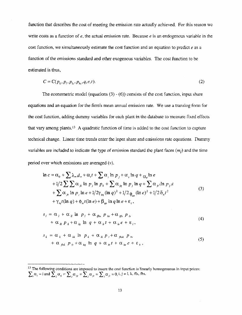
The econometric model (equations (3) - (6)) consists of the cost function, input share
equations and an equation for the firm's mean annual emission rate. We use a translog form for
the cost function, adding dummy variables for each plant in the database to measure fixed effects
that vary among plants.13 A quadratic function of time is added to the cost function to capture
technical change. Linear time trends enter the input share and emissions rate equations. Dummy
variables are included to indicate the type of emission standard the plant faces (mi) and the time
period over which emissions are averaged (v).
Inc = co + X Xd, + CC,t + , In pj + icn q + leIn e
+ 1/2 E Ex jk In pj In pk + I ajq In pj ln q + E ac jt (In pj)t
+ I a,, ln p, In e + 1/2yqq, (In q) 2 + 1/2 O (In e)2 + 1/2 68,t2
+ y,qt(ln q) + pt,t(In e) + qe ln q In e + e,
s I cL I + a 11 hi p I + x IJhs P hs + a fls P Is
+ aI k Pk+c(tq hI q + ccitt + alee + El,
S k = ak + a kk In P k + C Ik P I + ( fhsk P hs (5)
+a flsk P Is + a lq In q + (xktt + ake e + E kX
3 The following conditions are imposed to insure the cost function is linearly homogeneous in input prices:Z,jaX= landz,(c,j=jj cj,q =Ejxj, = Eja =jO,i,j=1,k,f1s,fhs.
13

lh e = ce +aeh n +X imi + I yimi(ln e*) (6)
+ 6iv + 6tt + Xi In Pi + 6tt + -e'
The estimated model includes input share equations only for labor and capital. This is
necessary because of the large number of zero values for inputs of low-sulfur and high-sulfur coal.
At the level of the generating unit only one type of coal is typically used, implying a zero cost
share for the alternative fuel type. To avoid the bias that zero shares would introduce in our
estimates we include only the share equations for generating capital and labor.
The estimation of abatement cost functions is further complicated by the fact that over half
of the units in our database exhibit non-cost-minimizing behavior in their choices of fuel at some
time during the sample period. Either as a result of long-term fuel contracts or of other
unobservable transaction costs associated with fuel switching, these units did not immediately
switch to low-sulfur coal when it appeared to be economic for them to do so. 14 In some cases
remaining in long-term contracts may have provided a hedge against price fluctuations. In other
cases utilities may have had little incentive to respond to price changes if fuel prices could be
passed on to consumers (Atkinson and Kerkvliet, 1989). In any event, these observations violate
the assumption of cost minimization implicit in the specification of the model and are therefore
excluded when we estimate the cost function.15
14 We tested to see if firms that are apparently violating cost minimizing behavior are bound by older contractsrelative to other firms, on the assumption that the older the contract the less likely it is to reflect current pricesfacing the firm. Although, the contract age of plants that are apparently not cost minimizing is longer, 6 monthsout of a average contract age of 5 years, this does not seem to be a large enough difference to account for all of thenon-cost minimizing behavior.
15 This results in eliminating some units for certain years, but still enables us to estimate a cost function for theseunits. They are therefore included in our calculation of the least cost solution.
14
The cost function, corresponding share equations and the emission rate equation are
estimated by Full Information Maximum Likelihood methods using panel data for the period
1985-1994. The stochastic disturbances in the estimating equations for any observation are
assumed to be correlated across equations.
Our interest centers on the marginal cost of achieving emissions rate e, which can, in turn,
be translated into a marginal cost function for tons of S0 2 . In general terms, the marginal cost of
emissions function is given by aC/ae, which is usually negative over observed ranges of emissions.
The negative of this function, - aC/ae, will henceforth be referred to as the marginal abatement
cost function. To describe the marginal cost of abating a ton of SO2 , the cost of a given
percentage reduction in the emissions rate can be converted into the equivalent reduction in tons
of S0 2.16
Data
Our data set consists of virtually all privately and publicly owned Phase I coal-fired
generating units, and all privately owned Phase II coal-fired units.17 These units are responsible
for 87% of all SO2 emissions produced by coal-fired power plants in 1985 and 85% of all
emissions in 1994. For each generating unit we compiled data on generating capital, abatement
capital, labor, and inputs of high and low-sulfur coal for 1985-94. The data also include the SO2
16 The marginal cost of a change in the SO2 emissions rate, e, at a particular value of e is defined as negative onetimes the product of the elasticity of total cost with respect to the emission rate, and the ratio of total cost to theobserved emissions rate, or -aC/ae = (-alnC/6lne)(C/e). The marginal cost of abating an additional ton of SO2ermissions, may be derived from the fact that e=SO2/MMBTU, where MMBTU is millions of BTUs of heat input.It follows that, -6C/aSO2 = -&C/3e (1/MMBTU) = (-alnC/alne)(C/(S02/MMBTU)) (l/MMBTU) = -(alnC/alne)(C/SO2 ).
17 The data set excludes all cooperatively-owned plants, which are subject to different reporting requirements thaneither privately or publicly owned plants.
15

emission rate standard facing the generating unit, its mean annual emission rate in pounds of SO2
per million Btus of heat input (mmBtu) and output in kilowatt hours. The input prices facing each
power plant complete the data set. (See Appendix A for a more complete description.)
To describe sulfur content we distinguish two classes of coal. Coal that when burned in a
standard boiler generates no more than 1.2 pounds of sulfur dioxide per million Btus of heat input
is defined as low-sulfur coal; all other is high-sulfur coal. This distinction is not entirely arbitrary.
Coal resulting in 1.2 pounds of sulfur dioxide or less is termed "compliance coal" due to its ability
to meet the original NSPS, in effect from 1971-1978. It also will meet Phase II emission
standards, on average.1 8 For a firm that purchased only high-sulfur coal, we use the average price
of high-sulfur coal in the state where the plant is located. In all cases, we use the contract price
rather than the spot price of coal.19
Results of the Estimation
To summarize the results of our estimation we evaluate the marginal abatement cost
function for each unit at 1985 and 1994 emission levels. Table 1 presents the mean and standard
deviation of the marginal cost of abating a ton of S0 2, when marginal abatement costs for
different units are weighted by SO2 emissions. In the 1994 time period, 89% of all the predicted
marginal abatement costs are significantly different from 0 at the 5% level.
18 An alternative approach to modeling the sulfur content of coal, used by Kolstad and Turnovsky (1995), is toallow plants to select sulfur content as a continuous attribute, given a hedonic price function for coal. Weattempted this approach, but were unable to obtain reliable estimates of hedonic price functions for each state andyear.
19 In 1985, 89% of all coal was purchased through long-term contracts rather than on the spot market. Althoughthis percentage has declined through time, 80% of all coal was still purchased through long-term contracts in1995. For this reason we use contract prices throughout the analysis.
16
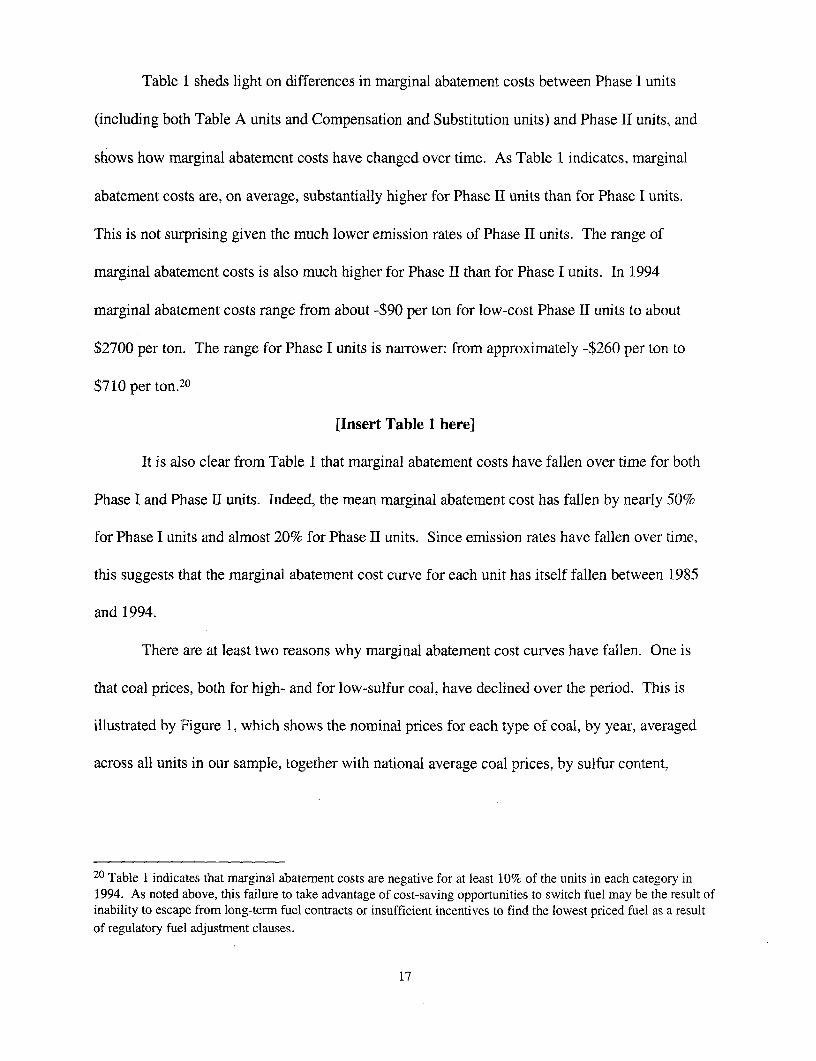
Table 1 sheds light on differences in marginal abatement costs between Phase I units
(including both Table A units and Compensation and Substitution units) and Phase II units, and
shows how marginal abatement costs have changed over time. As Table 1 indicates, marginal
abatement costs are, on average, substantially higher for Phase II units than for Phase I units.
This is not surprising given the much lower emission rates of Phase II units. The range of
marginal abatement costs is also much higher for Phase II than for Phase I units. In 1994
marginal abatement costs range from about -$90 per ton for low-cost Phase II units to about
$2700 per ton. The range for Phase I units is narrower: from approximately -$260 per ton to
$710 per ton.2 0
[Insert Table 1 here]
It is also clear from Table 1 that marginal abatement costs have fallen over time for both
Phase I and Phase II units. Indeed, the mean marginal abatement cost has fallen by nearly 50%
for Phase I units and almost 20% for Phase II units. Since emission rates have fallen over time,
this suggests that the marginal abatement cost curve for each unit has itself fallen between 1985
and 1994.
There are at least two reasons why marginal abatement cost curves have fallen. One is
that coal prices, both for high- and for low-sulfur coal, have declined over the period. This is
illustrated by Figure 1, which shows the nominal prices for each type of coal, by year, averaged
across all units in our sample, together with national average coal prices, by sulfur content,
20 Table 1 indicates that marginal abatement costs are negative for at least 10% of the units in each category in1994. As noted above, this failure to take advantage of cost-saving opportunities to switch fuel may be the result ofinability to escape from long-term fuel contracts or insufficient incentives to find the lowest priced fuel as a resultof regulatory fuel adjustment clauses.
17

computed for all utilities.21 Figure 1 indicates that the prices of both types of coal fell between
1985 and 1995; however, the price of low-sulfur coal fell faster. What Figure 1 does not show is
that the price of low-sulfur coal was lower than the price of high-sulfur coal for 20% of the units
in our sample in 1985 and for 25% of the units in our sample in 1994. Over the same period the
quantity of low sulfur coal delivered to electric utilities rose significantly. The second reason for a
fall in the marginal abatement cost curve is technical progress in abating sulfur dioxide emissions,
resulting in part from more general technical progress in electricity generation.
[Insert Figure 1 here]
How important are price changes and technical progress in explaining the fall in marginal
abatement cost curves? To answer this question Figure 2 plots marginal abatement cost curves
for a generating unit with average Phase I input and output characteristics using (a) 1985 fuel
prices and 1985 time trend, (b) 1985 fuel prices and 1995 time trend, (c) 1995 fuel prices and
1985 time trend (d) 1995 fuel prices and 1995 time trend and (e) 1995 fuel prices and 2010 time
trend. In all five curves output (Q) as well as all non-fuel input prices are held constant. The
effect of technological improvements, represented by the vertical distance between curves (a) and
(b) accounts for about 20 percent of the change of the MAC function, or a decline of about $50
per ton between 1985 and 1995. The effect of changes in fuel prices, represented by the vertical
21 The bars in this chart reflect differences in coal prices as they appear in our dataset. In computing the price oflow- (high-) sulfur coal we have weighted the price actually paid by plants that purchase low- (high-) sulfur bytheir heat input and have similarly weighted the predicted price of low- (high-) sulfur coal for plants thatpurchased only high- (low-) sulfur coal. The lines represent national average coal prices, which are computed byaveraging the prices paid only by firms that actually purchased each type of coal, including firms excluded fromour dataset. The resulting low-sulfur coal prices are slightly lower than our estimates. Our higher low-sulfur coalprices result from the fact that many plants in our data set faced with higher than average low-sulfur coal prices donot actually purchase low-sulfur coal. Therefore the average low-sulfur coal price in our dataset should be higherthan the national average.
18

distance between curves (b) and (d) accounts for the remaining 80 percent of the fall in the
marginal abatement cost function, a decline of about $200 per ton.
[Insert Figure 2 here]
This figure also demonstrates why marginal abatement costs computed at the plant's
actual level of emissions have fallen even as emissions have themselves declined. Without
technological change or changes in fuel prices, an average plant would move from point A in
1985 to Point B in 1995. MAC would increase as emissions were reduced by 6,000 tons. With
changes in fuel prices and technology, however, the unit moves to Point C where its marginal
abatement cost is only about half as large as it was originally.22 If the current trend in
technological improvements continues until the year 2010, this average unit's marginal abatement
cost will fall by an additional $100 ((d) to (e)).
IV. The Least Cost Solution and Potential Gains from Trade in the Long Run
A. Preferred Estimates of the Least Cost Solution
To estimate potential gains from allowance trading in the long run, we compute the least
cost solution to achieving the 8.95 million ton S02 cap in the year 2010. This requires that we
make assumptions about parameters that will shift the marginal abatement cost functions over
time-the rate of growth of electricity production (Q), fuel prices (pls and phs), and the rate of
technical progress. We must also determine the rate at which coal plants in existence in 1995 will
be retired from service, and must determine what SO2 emissions would have been in 2010 in the
absence of the CAAA.
22 It is important to keep in mind that the relative importance of technological change and fuel prices on anindividual unit's marginal abatement cost function depends greatly on where the unit is located. Generating unitslocated in areas that have had access to relatively inexpensive low-sulfur coal for some time would not see asubstantial drop in their marginal abatement cost functions due to changes in coal prices.
19
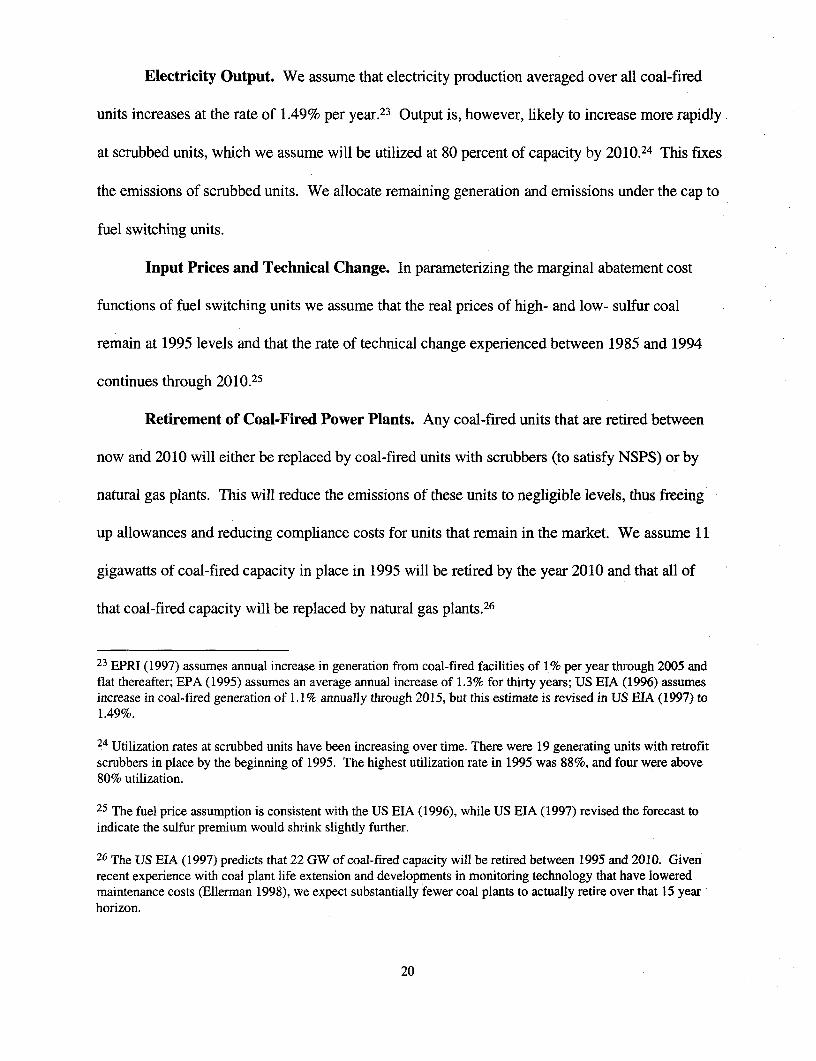
Electricity Output. We assume that electricity production averaged over all coal-fired
units increases at the rate of 1.49% per year.23 Output is, however, likely to increase more rapidly
at scrubbed units, which we assume will be utilized at 80 percent of capacity by 2010.24 This fixes
the emissions of scrubbed units. We allocate remaining generation and emissions under the cap to
fuel switching units.
Input Prices and Technical Change. In parameterizing the marginal abatement cost
functions of fuel switching units we assume that the real prices of high- and low- sulfur coal
remain at 1995 levels and that the rate of technical change experienced between 1985 and 1994
continues through 2010.25
Retirement of Coal-Fired Power Plants. Any coal-fired units that are retired between
now and 2010 will either be replaced by coal-fired units with scrubbers (to satisfy NSPS) or by
natural gas plants. This will reduce the emissions of these units to negligible levels, thus freeing
up allowances and reducing compliance costs for units that remain in the market. We assume 11-
gigawatts of coal-fired capacity in place in 1995 will be retired by the year 2010 and that all of
that coal-fired capacity will be replaced by natural gas plants.26
23 EPRI (1997) assumes annual increase in generation from coal-fired facilities of 1% per year through 2005 andflat thereafter; EPA (1995) assumes an average annual increase of 1.3% for thirty years; US EIA (1996) assumesincrease in coal-fired generation of 1.1% annually through 2015, but this estimate is revised in US EIA (1997) to1.49%.
24 Utilization rates at scrubbed units have been increasing over time. There were 19 generating units with retrofitscrubbers in place by the beginning of 1995. The highest utilization rate in 1995 was 88%, and four were above80% utilization.
25 The fuel price assumption is consistent with the US EIA (1996), while US EIA (1997) revised the forecast toindicate the sulfur premium would shrink slightly further.
26 The US EIA (1997) predicts that 22 GW of coal-fired capacity will be retired between 1995 and 2010. Givenrecent experience with coal plant life extension and developments in monitoring technology that have loweredmaintenance costs (Ellerman 1998), we expect substantially fewer coal plants to actually retire over that 15 yearhorizon.
20

Baseline Emissions. We compute baseline emissions-those that would have prevailed
absent Title IV-using 1993 emissions rates applied to 2010 levels of electricity production. We
believe that the declines in emission rates that occurred between 1985 and 1993 were primarily
the result of decreases in the price of low sulfur coal and would have happened in the absence of
Title IV.
Continuous Emissions Monitoring Data. An important feature of the 1990 CAAA is
that SO2 emissions must be measured by a continuous emissions monitoring system (CEMS)
rather than being estimated based on fuel consumption. Previous studies all use engineering
estimates of SO2 emissions. A comparison of the two measurement techniques reveals that, in
1995, CEMS emissions were about 7 percent higher than estimated emissions, implying that the
S02 cap is, in effect, 7 percent below the cap based on engineering formulas. To be consistent
with actual practice, we use CEMS data.
Compliance Costs in the Preferred Case
Under the above assumptions, the total annual cost of achieving the S0 2 cap of 8.95
million tons in 2010 is $1.04 billion (1995 dollars). Of this total, $380 million represents the cost
incurred by plants that fuel switch, which account for about 60% of reductions from baseline
emissions.27 For plants that have installed scrubbers, annualized capital costs are $382 million per
year and variable costs $274 million per year.
The marginal cost of emissions reduction, which should approximate long run permit
price, is $291 per ton of SO2 . This assumes that the marginal ton of SO2 is reduced via fuel
27 We have investigated the implied transportation of low-sulfur coal and found it to be a modest extension ofrecent trends in the increased use of low-sulfur coal.
21

switching, an assumption that is justified if one compares the cost of reducing SO2 by installing
retrofit scrubbers with the cost via fuel switching. Though the useful life of a retrofit scrubber is
likely to be close to 20 years (EPA, 1995), the investment decision should reflect current financial
and regulatory uncertainties in the industry, which call for a 10 year payback life (EPRI, 1997).
With this decision rule, the average cost per ton of reducing SO2 through additional retrofit
scrubbers is $406, which exceeds the marginal cost of SO2 reduction via fuel switching.
B. Comparisons and Sensitivity Analyses
Annual compliance costs of $1 billion per year are far lower than originally predicted when
the 1990 Clean Air Act Amendments were drafted. In fact, they are less than half of the estimates
of compliance costs expected by the EPA (1989, 1990). This raises two questions: Are our
estimates of compliance costs biased downward? If not, why are they so much lower than EPA's
original estimates of such costs?
The assumptions made above with regard to electricity generation and fuel prices are
likely to overstate, rather than understate costs. We assume, for example, the same rate of
growth in electricity generated by coal and a slower rate of retirement of coal-fired plants than
official predictions (US EIA 1997). The assumption that high- and low- sulfur coal prices remain
at their 1995 is also conservative-the Energy Information Administration (1997) predicts a
reduction in the low-sulfur premium below 1995 levels.
The one assumption that might bias our cost estimates downward is that technical
progress will continue from 1995 until 2010 at the same rate as between 1985 and 1994. If we
assume, at the other extreme, that technical progress stops in 1995, our estimate of compliance
costs rises to $1.51 million (1995 dollars) and our estimate of long-run allowance price to $436
per ton of S02. Even this extreme assumption puts our estimates of total compliance costs below
22

EPA's (1990) estimate of $2.5 - $6.0 billion (Table 2), and our estimate of marginal cost below
EPA's estimate of $579-$760 per ton.2 8
[Insert Table 2 here]
It is important for two reasons to understand why these estimates differ. One is to see
whether there is a systematic tendency to over-estimate the cost of environmental regulations.
That costs are systematically over-estimated has been alleged both by economists (Hammitt 1997)
and environmentalists, and is an especially timely issue in light of debates over the cost of
reducing greenhouse gases. The second reason is that the factors that explain why estimates of
compliance costs have fallen also explain why the costs of command-and-control approaches to
reducing SO2 have fallen and why the potential gains from allowance trading are also lower than
originally anticipated.29
One reason for EPA's high estimates of compliance costs is failure to foresee the
continued fall in the low-sulfur coal premium, as well as continuing technical progress in fuel
switching. To estimate the magnitude of these effects we re-compute the least cost solution using
1989 prices and technology.3 0 Both total and marginal abatement costs rise by about 90% (Table
2). When fuel switching determines the marginal cost of compliance, using 1989 fuel prices and
technology can produce marginal cost estimates approximately as large as those predicted when
Title IV was written. Total costs also increase, in part because a higher sulfur premium lowers
28 Recent engineering studies that acknowledge the use of low-sulfur coal for compliance have also identified thedeclining trend of marginal and annual costs of compliance (EPA (1995) and EPRI (1995,1997)).
29 Even in the absence of trading, Title IV allows finns unprecedented flexibility in selecting a method forcomplying with SO2 emission reduction goals. This increased flexibility is believed to have contributed to recentdeclines in low-sulfur fuel prices and the pace of innovation in fuel switching and scrubbing (Burtraw 1996).
30 We also assume that emissions are estimated based on fuel consumption, as they were in studies prior to thepassage of Title IV.
23
the percent of emissions reductions that can be obtained for free. Using 1989 prices and
technology only 21 percent of emissions reductions from plants that fuel switch are obtained by
realizing negative marginal abatement costs. This figure, however, rises to 57 percent in the
preferred scenario.31
Failure to foresee changes in prices and technical progress, however, does not explain all
of the difference in total cost estimates. Also important are differences in the baseline from which
emissions reductions are measured. In all of our calculations, we assume that the emission rates
(lbs. of S0 2/mmBtu) that would have prevailed absent the 1990 Clean Air Act Amendments are
those that prevailed in 1993. These are much lower than 1989 emission rates, hence the
reductions in emissions necessary to achieve the 8.95 million ton cap, by our calculations, are
much lower than imagined in 1989 (specifically, about 2 million tons lower). Holding MAC
curves constant, lowering the necessary reduction in emissions will lower total compliance costs.
Finally, EPA's estimates of compliance costs are higher than ours because they assumed
that more retrofit scrubbers would be built (37) than were actually constructed (28), because they
failed to foresee a 50% fall in the cost of scrubbing that we identify.
C. Potential Gains from Trade
We now consider the cost of meeting the S02 cap using a command and control approach,
and compute the potential gains from trade as the difference between this cost and the cost of
compliance under the least cost solution. Since the goal of Title IV is to achieve an average
emissions rate of 1.2 pounds of SO2 per million Btus of heat input, we model command and
31 While this estimate may seem high, we have evidence from 1995 and 1996 that utilities are realizing sucheconomic cost savings. In 1995 one-quarter of a potential $443 million in savings from fuel switching wererealized. In 1996, half of $644 million in potential savings were realized. We believe that increased competitionin the electric utility industry will motivate generators to take advantage of these savings.
24

control as a uniform performance standard that is designed to achieve the same level of emissions
as the trading program.3 2
For our preferred case, we estimate the potential gains from trade compared to the
command and control scenario to be $784 million (43% of the cost of command and control).
While these gains constitute a substantial fraction of the cost of command and control, they are
not as large as were originally predicted. The GAO (1994), for example, estimated that a per-unit
cap on emissions would cost approximately $5.3 billion annually and the reduction in costs from
efficient trading to be $3.1 billion (about 60% of this figure).
The explanation for our more modest estimates of trading gains is clear-the factors that
have caused marginal abatement costs to fall to a large extent also would have lowered the costs
of achieving the S02 emissions cap via command and control. These include the fall in the price
of low sulfur coal and, to some extent, technical improvements that have facilitated fuel
switching.3 3 It should also be noted that, in addition to lowering marginal abatement cost curves
(see Figure 3), the fall in low sulfur coal prices has made marginal abatement cost curves more
homogenous. This is because costs of transporting low sulfur coal to more distant locations, for
example, the East and Southeast, has fallen rendering differences in transportation cost a less
important component of the overall cost of fuel switching. Since a major source of trading gains
32 The uniform emission rate standard does not take into account the fact that some units may face unrealized"economic" emission reductions beyond those mandated by the standard. Therefore, emissions are lower under theuniform standard than they are under a trading prograrn, which provides firms with higher abatement costs theflexibility to capture the slack in the effective emission constraint at other firms (Oates, Portney and McGartland1989).
33 Some of the technological developments in fuel blending may not have occurred under a uniform emissionsstandard since blending of coals with different sulfur contents by itself, i.e. without the option of purchasingallowances, generally would not be sufficient to achieve the required emission reductions. Similarly, there wouldhave been less incentive to improve the performance of scrubbing equipment under a uniform emission ratestandard and the witnessed improvements may not have been realized. To the extent that the effects of theallowance trading program on technological change in emissions reduction are reflected in our data, our estimates
25

is differences in marginal abatement cost curves among units in the market, this increased
homogeneity is also responsible for low gains from trade.
The relatively modest potential trading gains reflected in our results sl ould not be
interpreted as a criticism of the allowance market, but they are likely to have an impact on market
performance. If potential gains from trade are small and transactions costs of using the market
are substantial, utilities will be less eager to trade allowances. In the next section, we analyze the
performance of the SO2 allowance market in 1995 and 1996 to determine both the potential gains
from trade under a perfectly functioning market and how much of these gains actually have been
realized.
V. The Performance of the Allowance Market in 1995 and 1996
In 1995 the aggregate emissions of Phase I units were approximately 5.3 million tons,
rising to 5.44 million tons in 1996. To compute the least cost method of achieving these
emissions levels we parameterize marginal abatement cost functions for each unit using actual
output levels and input prices. Technical progress is assumed to occur at the same annual rate as
observed between 1984 and 1995. We take as our baseline 1993 emission rates, which we apply
to 1995 and 1996 electricity generation to predict emissions in the absence of Title IV.
The least cost solution yields a common marginal abatement cost for the last ton emitted
among units that fuel switch and a set of efficient emission levels for all generating units. To
compute total costs we integrate each unit's marginal abatement cost curve from baseline
emissions to emissions under the least cost solution. The total cost of actual emissions in each
of the costs of a uniform emission rate standard and the potential gains from trade are likely understated.
26

year is computed analogously, except that integration under the MAC curve occurs from baseline
emissions to actual 1995 and 1996 emissions.34
[Insert Table 3 here]
The least cost solution to achieving 1995 emissions, including the capital and variable
costs of scrubbing ($496 million), is $552 million (1995 dollars) (see Table 3). The estimated
actual cost of achieving 1995 emissions is considerably higher-$832 million. This suggests that
$280 million of potential cost savings were unrealized in the first year of the allowance market.
Our estimate of the actual costs is close to estimates obtained by Ellerman et al. (1997) of actual
compliance costs ($728 million) based on a survey of the industry. We consider the difference
between these estimates and the least cost solution as evidence that there were unrealized gains
from trade in 1995.
In 1996 performance under the program did not change dramatically. The least cost
solution to achieving 1996 emissions is $571 million (1995 dollars). The estimated actual cost of
achieving 1996 emissions increased slightly from the previous year, partly due to increased
utilization of scrubbed units. This suggests that $339 million of potential cost savings were
unrealized in the second year of the allowance market.
We note that the marginal cost of the last ton emitted in the least-cost solution ($101 in
1995 and $71 in 1996) is close to the price at which allowances were trading (around $90). The
equality of these numbers does not, however, demonstrate that the market was operating
efficiently: The two could be equal even if many participants opted out of the market, which was
in fact the case.
34 Emission rates are based on DOE-EIA engineering estimates not CEMS data. Because both the heat input andSO2 emissions estimated by the DOE-EIA are lower than the CEMS measurements the estimated emission ratesare equal on average.
27

Although the allowance market in its first years of operation failed to achieve the least
cost solution, it is possible that it was more efficient than a command and control approach to
achieving emissions. The cost of the uniform emissions rate standard necessary to achieve actual
1995 emissions is approximately $800 million, slightly less than our point estimate of actual
emissions costs (Table 3). What this suggests is that the uniform performance standard, although
it fails to equalize MAC per ton of SO2 , is no less efficient than the actual pattern of emissions
chosen by utilities. It also implies potential gains from trade (potential cost savings of trading
over command and control) of $250 million, or about one-third of the costs of command and
control.
The failure of the allowance market to achieve the least-cost solution in 1995 and 1996 is
neither surprising nor alarming. Title IV represents a dramatic departure from traditional
environmental regulation. It requires utilities to manage a financial asset--emission allowances--
for which there is no precedent. It also requires a well-functioning market in allowances, which
takes time to establish. There is evidence that allowance trades are growing in volume.
Economically significant trades between separate utility holding companies have doubled every
year since the inception of the program through 1997, which suggests that utilities are increasingly
taking advantage of the allowance market as a means to reduce compliance costs (Kruger and
Dean, 1997). In addition the number of allowances used for compliance that were obtained
through inter-firm transactions increased by 50% between 1995 and 1996.
VI. Conclusions
When the market for sulfur dioxide allowances was envisioned in the late 1980's, the cost
of complying with the proposed SO2 cap was thought to be much higher than it has, in fact,
turned out to be. Likewise, the potential trading gains associated with the market were predicted
28

to be much higher than the estimates presented above. The lower trading gains that we predict
for the allowance market in the long run are largely the result of two factors--declines in the price
of low sulfur coal and improvements in technology that have lowered the cost of fuel switching.
These factors have lowered the gains from trade in two ways. First, they have lowered marginal
abatement cost curves for most generating units, which has lowered the cost of achieving the cap
via a uniform performance standard, as well as the cost of achieving the cap through allowance
trading. Second, because spatial differences in coal prices have been reduced, marginal abatement
cost curves have become more homogeneous, which has also lowered the gains from trade.
Our results have several important lessons for policy makers as they consider adopting an
allowance trading approach to regulating other utility emissions such as nitrogen oxides (NOx)
and greenhouse gases. First, our findings lend support to the theory that the costs of compliance
with regulation are often overestimated ex ante. We show that estimates of the costs of
compliance with the SO2 reduction goals under Title IV have fallen substantially over time due to
a combination of unanticipated declines in coal prices and technical change. This suggests that
attempts to estimate the future costs of other pollution control programs may be similarly flawed,
especially given the difficulty in forecasting future trends in technological change. This
technology forecasting task is made more complicated by the introduction of greater competition
in electricity markets, which is expected to accelerate the pace of technical change.
Second, our results suggest that, in designing an allowance market, it is important for
policy makers to consider the source of trading gains and how these gains might change over
time. The source of trading gains in the SO2 allowance market is spatial differences in the price of
high v. low sulfur coal. As these price differences have diminished, so have potential trading
gains. In the market for CO2 there are, initially, likely to be large trading gains because coal-fired
29

power plants, by converting to natural gas, can reduce their CO2 emissions at a lower cost than
oil- and gas-fired plants. Once this conversion is completed, however, trading gains within the
electric utility industry will diminish.
Lastly, our results suggest that it will take time for allowance markets to mature and,
therefore, for the potential gains from trade to be realized. We show that, on the whole, the
market failed to realize potential gains from trade in 1995 or 1996. The reluctance of many firms
in the utility industry to take advantage of the allowance market may be a result of features of
utility regulation that have limited incentives to participate in the market. As competition
increases within the generation segment of the industry, and as we enter the second phase of the
allowance program, we expect to see greater use of the market to reduce the costs of
environmental compliance. Formal trading in the SO2 allowance market may not achieve large
cost savings compared to a uniform performance standard. The flexibility of the trading program,
though, has encouraged utilities to capitalize on advantageous trends, such as changing fuel prices
and technological innovation that might have been delayed or discouraged by traditional
regulatory approaches. The SO2 program shows that a market in tradable emission rights is,
indeed, feasible. As the electric utilities industry becomes more competitive, one would expect to
see the advantage of emission trading programs for other pollutants to become more evident.
30
References
Atkinson S. and J. Kerkvliet. 1989. "Dual Measures of Monopoly and Monopsony Power: AnApplication to Regulated Electric Utilities," The Review of Economics and Statistics71(2), pp. 250-257.
Bohi, D. R. 1994. "Utilities and State Regulators Are Failing to Take Advantage of EmissionAllowance Trading," The Electricity Journal 7(2), pp. 20-27.
Bohi, Douglas R. and Dallas Burtraw. 1992. "Utility Investment Behavior and the EmissionTrading Market," Resources and Energy 14(1/2), pp. 129-156.
Burtraw, Dallas. 1996. "Cost Savings Sans Allowance Trades? Evaluating the S02 EmissionTrading Program to Date," Contemporary Economic Policy 14(2), pp. 79-94.
Dallas Burtraw, Alan J. Krupnick, Erin Mansur, David Austin, and Deirdre Farrell. 1998. "TheCosts and Benefits of Reducing Acid Rain," Contemporary Economic Policy,Forthcoming.
Cowing, Thomas, Jeffrey Small and Rodney Stevenson. 1981. "Comparative Measures of TotalFactor Productivity in the Regulated Sector: The Electric Utility Industry," in ProductivityMeasurement in Regulated Industries edited by Thomas Cowing and Rodney Stevenson,New York: Academic Press, pp. 161-177.
Ellerman, Denny. 1998. "Note on The Seemingly Indefinite Extension of Power Plant Lives, APanel Contribution," The Energy Journal 19: 129 - 132.
Ellerman, A. Denny and Juan Pablo Montero. 1996. "Why Are Allowance Prices so Low? AnAnalysis of S02 Emissions Trading Program," MIT-CEEPR working paper 96-001.
Ellerman, A. Denny, Richard Schmalensee, Paul L. Joskow, Juan Pablo Montero, and ElizabethM. Bailey. 1997. "Emissions Trading under the U.S. Acid Rain Program: Evaluation ofCompliance Costs and Allowance Market Performance," MIT Center for Energy andEnvironmental Policy Research (Ninth Draft: August 19).
Electric Power Research Institute (EPRI). 1997. SO2 Compliance and Allowance Trading:Developments and Outlook, TR-107891, prepared by Keith White, Palo Alto, CA (FinalReport: September).
Electric Power Research Institute (EPRI). 1996. Coal Supply and Transportation MarketsDuring Phase One: Change, Risk and Opportunity, TR-105916, prepared by James N.Heller and Stan Kaplan, Fieldston Company, Inc. (Final Report, January).
31
Electric Power Research Institute (EPRI). 1995. The Emission Allowance Market and ElectricUtility S02 Compliance in a Competitive and Uncertain Future, TR-105490, prepared byKeith White, Energy Ventures Analysis, Inc., and Van Horn Consulting. Palo Alto, CA(Final Report: September).
Fullerton, Don, Shaun P. McDermott and Jonathan P. Caulkins. 1997. "Sulfur DioxideCompliance of a Regulated Utility," Journal of Environmental Economics andManagement, vol. 34, no. 1 (September), 32-53.
Gollop, F. and M. Roberts. 1983. "Environmental Regulations and Productivity Growth: TheCase of Fossil-Fueled Electric Power Generation," Journal of Political Economy 91, pp.654-674.
Gollop, F. and M. Roberts. 1985. "Cost-Minimizing Regulation of Sulfur Emissions: RegionalGains in Electric Power." Review of Economics and Statistics 67, pp. 81-90.
Goulder, Lawrence H., Ian W. H. Parry and Dallas Burtraw, 1997. "Revenue-Raising vs. OtherApproaches to Environmental Protection: The Critical Significance of Pre-Existing TaxDistortions," RAND Journal of Economics, (Winter), forthcoming.
Hammitt, James. 1997. "Stratospheric Ozone Depletion," in Economic Analysis at EPA:Assessing Regulatory Impact, Richard Morgenstem, ed., Washington, DC: Resources forthe Future.
Kalagnanam, Jayant and Farasat Bokhari. 1995. "A Market Simulation-based Cost Module,"Department of Engineering and Public Policy, Carnegie Mellon University, mimeo.
Kolstad, Charles D. and Michelle H. L. Tumovsky. 1995. "Cost Functions and Nonlinear Prices:Estimating A Technology with Quality-Differentiated Inputs," University of
California, Santa Barbara, Department of Economics, mimeo.
Kruger, Joseph, and Melanie Dean. 1997. "Looking back on SO 2 Trading: What's Good for theEnvironment Is Good for the Market," Public Utilities Fortnightly, (August).
Oates, Wallace E., Paul R. Portney and Albert M. McGartland. 1989. "The Net Benefits ofIncentive-Based Regulation: A Case Study of Environmental Standard Setting," AmericanEconomic Review 79, pp. 1233-1242.
Rose, Kenneth. 1997. "Implementing an Emissions Trading Program in an EconomicallyRegulated Industry: Lessons from the SO2 Trading Program," in Market BasedApproaches to Environmental Policy: Regulatory Innovations to the Fore, Richard F.Kosobud and Jennifer M. Zimmerman (eds.), New York: Van Nostrand Reinhold.
32

Rubin, Jonathan D. 1996. "A Model of Intertemporal Emission Trading, Banking, andBorrowing," Journal of Environmental Economics and Management, 31 (3),(November), 269-286.
Siegel, Stuart A. 1997. "Evaluating the Cost Effectiveness of the Title IV Acid Rain Provisions ofthe 1990 Clean Air Act Amendments," Carnegie Mellon University Dissertation (May).
Temple, Barker and Sloane, Inc. (TBS). 1983. "Evaluation of H.R. 3400 The'SikorskilWaxman' Bill for Acid Rain Abatement, prepared for the Edison ElectricInstitute, September 20.
U.S. Energy Information Administration (EIA). 1982-1996. Form EIA-767, U.S. Department ofEnergy.
U.S. Energy Information Administration (EIA). 1985-1995. Electric Plant Cost and PowerProduction Expenses.
U.S. Energy Information Administration (EIA). 1985-1996. Monthly Report of Cost and Qualityof Fuels for Electric Plants.
U.S. Energy Information Administration (US EIA). 1996-1997. Annual Energy Outlook
U.S. Environmental Protection Agency (EPA). 1989. "Economic Analysis of Title V (sic) (AcidRain Provisions) of the Administration's Proposed Clean Air Act Amendments," Preparedby ICF Resources Incorporated (September).
U.S. Environmental Protection Agency (EPA). 1990. "Comparison of the Economic Impacts ofthe Acid Rain Provisions of the Senate Bill (S. 1630) and the House Bill (S. 1630),"Prepared by ICF Resources Incorporated (July).
U.S. Environmental Protection Agency (EPA). 1995. "Economic Analysis of The Title IVRequirements of the 1990 Clean Air Act Amendments," prepared by ICF ResourcesIncorporated (Final Report: September).
U.S. Environmental Protection Agency (EPA). 1996. "The Sulfur Dioxide (SO2 ) AllowanceTrading Program: The First Five Years," Acid Rain Division (January 19).
U.S. Federal Energy Regulatory Commission (FERC). 1982-1996. FERC Form 1.
U.S. Government Accounting Office (GAO). 1994. "Air Pollution: Allowance Trading Offersan Opportunity to Reduce Emissions at Less Cost," GAO/RCED-95-30, Washington,D.C., 1994
33
U.S. Office of Technology Assessment (OTA). 1983. "An Analysis of the 'SikorskilWaxman'Acid Rain Control Proposal: H.R. 3400, The National Acid Deposition Control Act of1983, Staff Memorandum (revised July 12).
Whitman, Requardt and Associates. 1995. The Handy-Whitman Index of Public UtilityConstruction Costs, Baltimore, Maryland (January).
Winebrake, J. J., M. A. Bernstein, and A. E. Farrell. 1995. "The Clean Air Act's sulfur dioxideemissions market: Estimating the costs of regulatory and legislative intervention," Resourceand Energy Economics, 17, (November), 239-260.
Yellen, Janet, "Testimony of Dr. Janet Yellen, Chair, White House Council of EconomicAdvisors, Before the House Commerce SubCommittee on Energy and Power, on theEconomics of the Kyoto Protocol, March 1998.
34
Appendix A
Data for estimating the generator unit level cost function (information on the levels of inputsand output) come from the Energy Information Administration's form EIA-767 and the FederalEnergy Regulatory Commission's Form 1 for the period 1985 to 1996. Electric utility plantcapital stock comes from Form 1 for the period 1982 to 1996. Prior to this, capital stock datacome from the Energy Information Administration's annual report Electric Plant Cost and PowerProduction Expenses (Expenses) and precursors to this report. Coal price information comesfrom the Monthly Report of Cost and Quality of Fuels for Electric Plants (Monthly Report). Thefollowing list describes each of the individual variables needed in the cost function.
Q: Output. Electrical generation (kWh) by generating unit. Source: EIA-767.
ph: Price of high sulfur fuel. Following the example of Gollop and Roberts (1983, 1985), theprice of high sulfur fuel is the weighted average price, in cents per million Btus, of high sulfur fuelbought by the utility that owns the generator. An emission boundary of 1.2 lbs. of S0 2 per
million Btus of heat input is used to differentiate low and high sulfur coal. If the utility bought nohigh sulfur fuel then the price is equal to the price of low sulfur fuel bought by the utilitymultiplied by the ratio of high to low sulfur coal prices in the state where the plant is located.Source: Monthly Report.
pl,: Price of low sulfur fuel. Measured in the same manner as the price of high sulfur fuel.Source: Monthly Report.
pi: Wage Rate. The utility's total labor expenditures divided by the sum of the total number offull-time employees and one-half of the number of part-time and temporary employees workingfor the utility. Publicly owned plants' wage rates are equal to the average wage rate of privatelyowned plants in the state where the plant is located or the region surrounding the state if noprivately owned plants are located in the same state. Source: Form 1
Pk: The rental price of generation capital. The rental price of generation capital is equal to theutility's cost of capital plus depreciation rate, adjusted for changes in the cost of construction(Cowing et al. 1981). That is,
pk = (Ri + DE)H1Wi,
where R is the utility's cost of capital, and DE is the depreciation rate and 1HW is the Handy-Whitman index of electric utility construction costs adjusted to reflect a base year of 1990. Thefinancial cost of capital for privately owned plants is estimated as the sum of the long-term debtinterest rate, the preferred stock dividend rate, and the required return on equity capital, whereeach factor is weighted by its respective capital structure proportion. The financial cost of capitalfor publicly owned plants is equal to the long term debt interest rate reported in Moody'sMunicipal and Government Manual. Data for jointly owned plants comes from the utility
35

indicated as the operator by EIA-767. The depreciation rate is assumed to be 5 percent and it isapplied to the undepreciated value of capital stock remaining in each year. This is based on adecay pattern defined by the 1.5 declining balance method and a 30 year asset life. Source: Form1 and The Handy-Whitnan Index of Public Utility Construction Costs.
e*: Emission Standard. The emission standard, in pounds of S0 2 per million Btu of heat input.
Source: EIA-767.
e: Average Emission Rate. The annual average emission rate for each utility plant. Source:Calculated by the Energy Information Administration from information in EIA-767.
k: Generation Capital Stock. The capital stock for each plant is calculated as follows:
CSi = (CSi-1) + NIi/HWi i = 1951,..., 1995,
where CSi is the adjusted capital stock for year i. Nli is the net investment for year i, DE is the
depreciation rate and HWi the Handy-Whitman index for year i adjusted to reflect a base year of
1990. The plant's net capital stock is equal to the initial investment in buildings and equipmentplus the costs of additions minus the value of retirements, expenditures on flue gas desulfurizationcapital stock and depreciation. Each generator's capital stock is the product of the plant's capitalstock and the generator unit's share of the plant's total generation capacity. Source: Expenses,EIA-767 and Form 1.
Generation Capital Expenditure. The product of the deflated generation capital stock and therental price of generation capital.
Labor Expenditure: The product of the wage rate and the total number of employees workingat the plant multiplied by the generator's share of the plant's total generation capacity.
High Sulfur Fuel Expenditure: The product of heat input from high sulfur coal, in millions ofBtus, and the price of high sulfur fuel. The type of fuel burned by the generating unit is de-termined from the unit's S0 2 emission rate before SO2 removal.
Low Sulfur Fuel Expenditure: The product of heat input from low sulfur coal, in millions ofBtus, and the price of low sulfur coal.
36
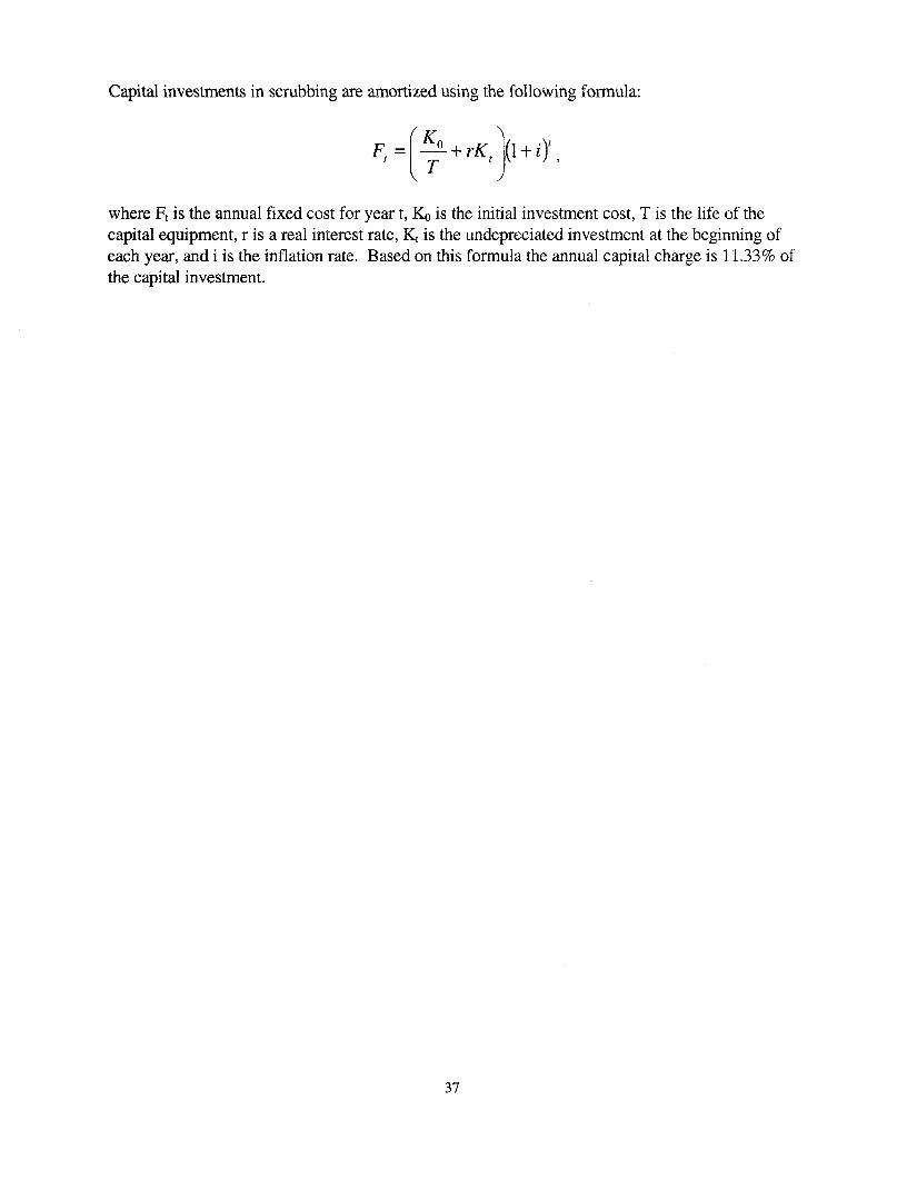
Capital investments in scrubbing are amortized using the following formula:
Ft=K T+rKtj(I+i),
where F, is the annual fixed cost for year t, Ko is the initial investment cost, T is the life of thecapital equipment, r is a real interest rate, Kt is the undepreciated investment at the beginning ofeach year, and i is the inflation rate. Based on this formula the annual capital charge is 11.33% ofthe capital investment.
37

Table 1: 1985 and 1994 Weighted Average Marginal Abatement Costs and S02 EmissionRates for Coal-Fired Units without Scrubbers
Emission Rate 10th Percentile 90th(lbs/mmBtu) Mean MAC Std. Dev. Percentile
1985 Phase I 3.65 $250 $485 $7 $582
Table A 4.09 $164 $308 -$1 $401
Comp. & Sub 1.97 $604 $812 $57 $1108
Phase II 1.33 $1332 $1836 $183 $3924
Total 2.45 $811 $1467 $51 $2636
1994 Phase I 2.82 $121 $475 -$264 $705
Table A 3.15 $104 $370 -$149 $431Comp. & Sub 1.47 $190 $763 -$293 $1499
Phase II 1.22 $1092 $2469 -$88 $2717
Total 1.90 $680 $1958 -$182 $1935*Emission Rates are weighted by total heat input and Marginal Abatement Costs are weighted by total S02 emissions. Figures are based on both units thatwere included and excluded from the costs function estimation in order to make comparisons between years meaningful.
38
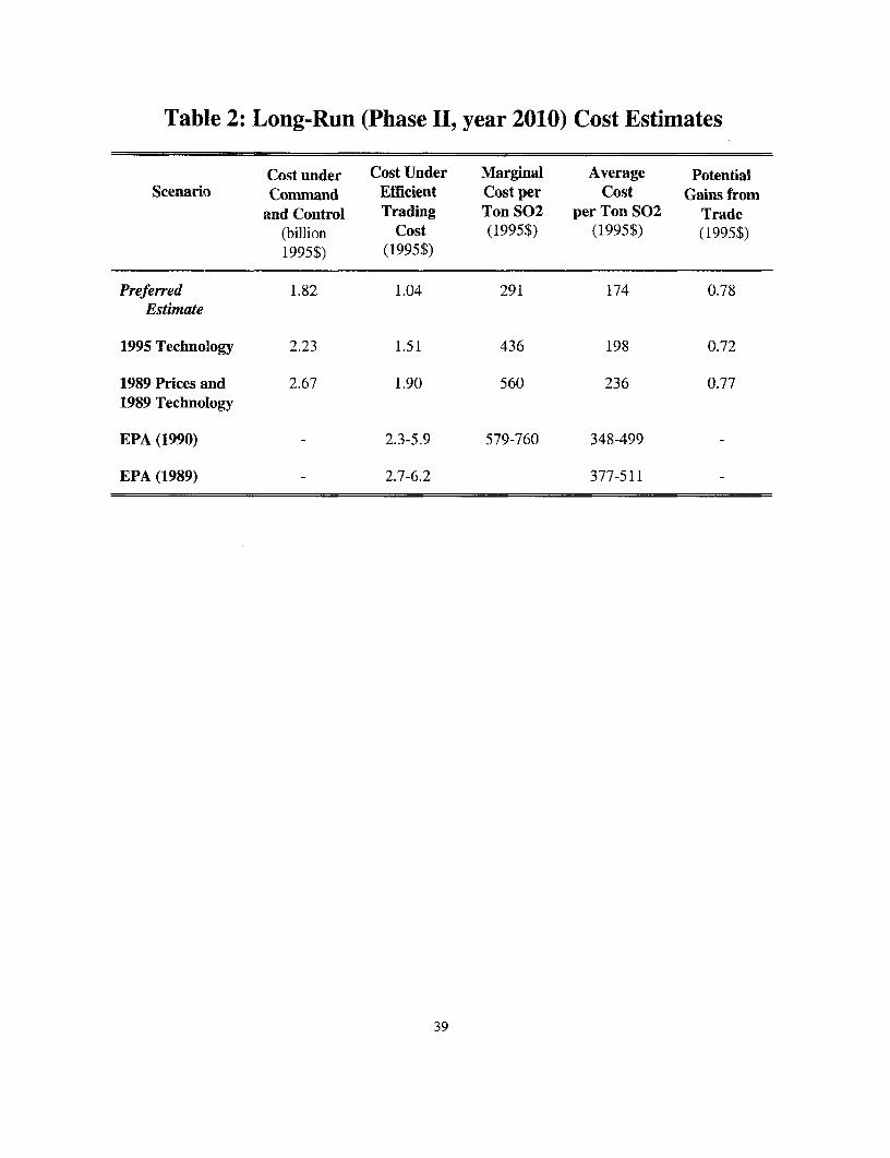
Table 2: Long-Run (Phase II, year 2010) Cost Estimates
Cost under Cost Under Marginal Average PotentialScenario Command Efficient Cost per Cost Gains from
and Control Trading Ton S02 per Ton S02 Trade(billion Cost (1995$) (1995$) (1995$)1995$) (1995$)
Preferred 1.82 1.04 291 174 0.78Estimate
1995 Technology 2.23 1.51 436 198 0.72
1989 Prices and 2.67 1.90 560 236 0.771989 Technology
EPA (1990) - 2.3-5.9 579-760 348-499
EPA (1989) - 2.7-6.2 377-511
39

Table 3: Phase 1 (1995 and 1996) Annual Total Cost
Command Efficient Potential Gainsand Control Trading MAC from Trade
(million (million 1995$) (1995$) (million 1995$)1995$)
1995
Preferred Estimate 802 552 101 250
Actual compliance 832 nla 280
1996
Preferred Estimate 777 571 71 206
Actual compliance 910 n/a 339
40

Figure 1: Low-Sulfur and High-Sulfur Coal Prices
200
190~-_
180 _Low Sulfur Coa~170 P_ ____-________ _ Pce
41________________ ______________ High SulfurCoal~160
~150 ~ 4-NationalLow1-140 ~~~~~~~~~~~~~~~~~~~~Sulfur Coal Price
Z U National Highw 130 A _Sulfur Coal Price
120
110
1985 1986 1987 1988 1989 1990 1991 1992 1993 1994 1995
41

Figure 2: The Effect of Changes in Fuel Prices and TechnicalChange on Marginal Abatement Cost Functions
$
600
500 el /
400 1e
300
200
100100 - ) 1995 Fuel Prices -~~~~~~1 99 51995 Time|
- )1995 Fuel Prices - 2010 Timee
_ - I | tc[ f tans S(220000 22000 24000 26000 28000 30000
42

Policy Research Working Paper Series
ContactTitle Author Date for paper
WPS1 952 Enterprise Isolation Programs in Simeon Djankov August 1998 R. VoTransitiorn Economies 33722
WPS1 953 Trade Policies and Incentives in Garry Pursell August 1998 L. TabadaIndian Acriculture: Methodology, 36896Background Statistics and Protection,and Incentive Indicators, 1965-95-Background Paper 1, Sugar andSugarcarne
WPS1954 Politicians and Firms in Seven Stijn Claessens August 1998 R. VoCentral and Eastern European Simeon Djankov 33722Countries
WPS1955 Appraising Workfare Programs Martin Ravallion August 1998 P. Sader33902
WPS1956 Benefit Incidence and the Timing Peter Lanjouw August 1998 P. Saderof Program Capture Martin Ravallion 33902
WPS1957 Bidding for Concessions Michael Klein August 1998 J. Dytang37161
WPS1958 Total Strangers or Soul Mates? J. Luis Guash August 1998 J. TroncosoAntidumping and Competition Sarath Rajapatirana 37826Policies in Latin America and theCaribbean
WPS1959 Is There a Credit Crunch in Wei Ding August 1998 F. FernandesEast Asia? Ilker Domac 80453
Giovanni Ferri
WPS1960 Calm After the Storms: income Francisco H. G. Ferreira August 1998 G. ilogonDistribution in Chile, 1987-94 Julie A. Litchfield 33732
WPS1961 Protecting the Environment and the Gunnar S. Eskeland August 1998 C. BernardoPoor: A Public Goods Framework Chingying Kong 31148Appliecl to Indonesia
WPS1962 The Political Economy of George R, G. Clarke August 1998 P. Sintim-AboagyePrivatization: An Empirical Analysis Robert Cull 38526of Bank Privatization in Argentina
WPS1963 Commodity Risk Management and Donald F. Larson August 1998 P. KokilaDevelopment Panos Varangis 33716
Nanae Yabuki
WPS1964 Public investment and Economic Ulrich Lachler August 1998 C. LazcanoGrowth in Mexico David Alan Aschauer 37776

Policy Research Working Paper Series
ContactTitle Author Date for paper
WPS1965 Manufacturing Firms in Developing James Tybout August 1998 L. TabadaCountries: How Well Do They Do, 36869and Why


