

Climate Change 2007:Synthesis Report
Summary for Policymakers
An Assessment of the Intergovernmental Panel on Climate Change
This summary, approved in detail at IPCC Plenary XXVII (Valencia, Spain, 12-17 November 2007), represents theformally agreed statement of the IPCC concerning key findings and uncertainties contained in the Working Groupcontributions to the Fourth Assessment Report.
Based on a draft prepared by:
Lenny Bernstein, Peter Bosch, Osvaldo Canziani, Zhenlin Chen, Renate Christ, Ogunlade Davidson, William Hare, SaleemulHuq, David Karoly, Vladimir Kattsov, Zbigniew Kundzewicz, Jian Liu, Ulrike Lohmann, Martin Manning, Taroh Matsuno,Bettina Menne, Bert Metz, Monirul Mirza, Neville Nicholls, Leonard Nurse, Rajendra Pachauri, Jean Palutikof, MartinParry, Dahe Qin, Nijavalli Ravindranath, Andy Reisinger, Jiawen Ren, Keywan Riahi, Cynthia Rosenzweig, MatildeRusticucci, Stephen Schneider, Youba Sokona, Susan Solomon, Peter Stott, Ronald Stouffer, Taishi Sugiyama, Rob Swart,Dennis Tirpak, Coleen Vogel, Gary Yohe

Summary for Policymakers
2
Introduction
This Synthesis Report is based on the assessment carriedout by the three Working Groups of the IntergovernmentalPanel on Climate Change (IPCC). It provides an integratedview of climate change as the final part of the IPCC’s FourthAssessment Report (AR4).
A complete elaboration of the Topics covered in this sum-mary can be found in this Synthesis Report and in the under-lying reports of the three Working Groups.
1. Observed changes in climate andtheir effects
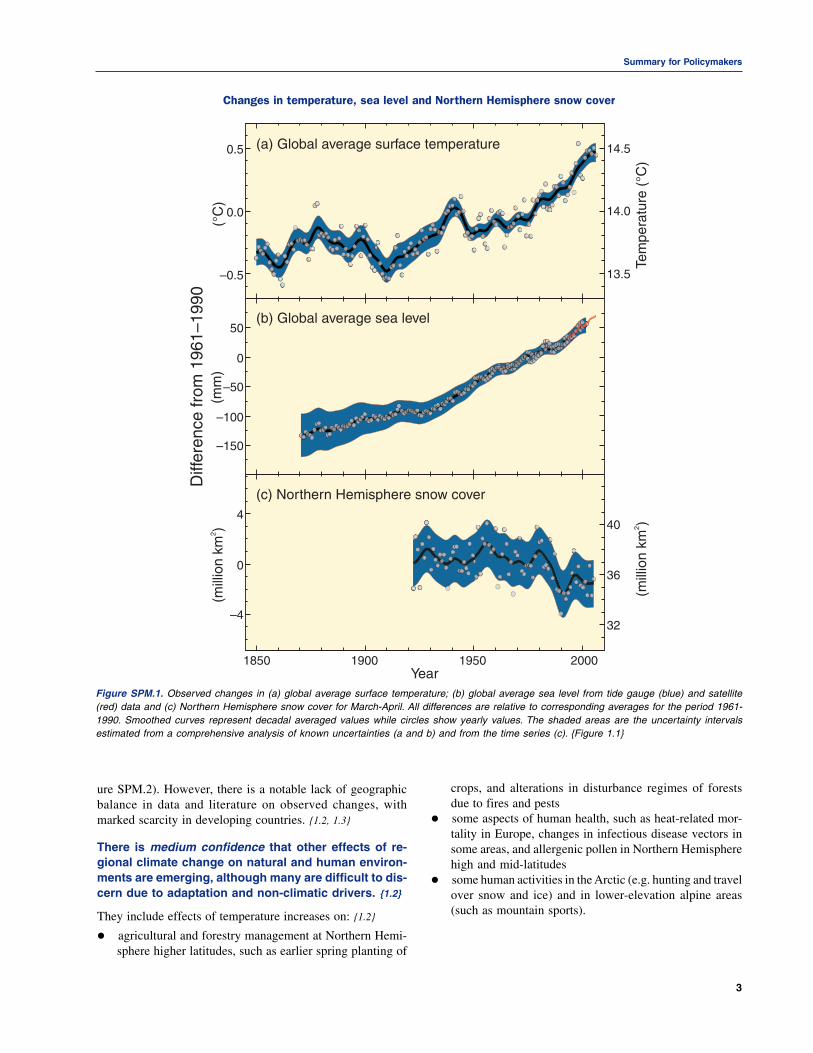
Warming of the climate system is unequivocal, as isnow evident from observations of increases in globalaverage air and ocean temperatures, widespread melt-ing of snow and ice and rising global average sea level(Figure SPM.1). {1.1}
Eleven of the last twelve years (1995-2006) rank amongthe twelve warmest years in the instrumental record of globalsurface temperature (since 1850). The 100-year linear trend(1906-2005) of 0.74 [0.56 to 0.92]°C1 is larger than the cor-responding trend of 0.6 [0.4 to 0.8]°C (1901-2000) given inthe Third Assessment Report (TAR) (Figure SPM.1). The tem-perature increase is widespread over the globe and is greaterat higher northern latitudes. Land regions have warmed fasterthan the oceans (Figures SPM.2, SPM.4). {1.1, 1.2}
Rising sea level is consistent with warming (FigureSPM.1). Global average sea level has risen since 1961 at anaverage rate of 1.8 [1.3 to 2.3] mm/yr and since 1993 at 3.1[2.4 to 3.8] mm/yr, with contributions from thermal expan-sion, melting glaciers and ice caps, and the polar ice sheets.Whether the faster rate for 1993 to 2003 reflects decadal varia-tion or an increase in the longer-term trend is unclear. {1.1}
Observed decreases in snow and ice extent are also con-sistent with warming (Figure SPM.1). Satellite data since 1978show that annual average Arctic sea ice extent has shrunk by2.7 [2.1 to 3.3]% per decade, with larger decreases in summerof 7.4 [5.0 to 9.8]% per decade. Mountain glaciers and snowcover on average have declined in both hemispheres. {1.1}
From 1900 to 2005, precipitation increased significantlyin eastern parts of North and South America, northern Europeand northern and central Asia but declined in the Sahel, the
Mediterranean, southern Africa and parts of southern Asia.Globally, the area affected by drought has likely2 increasedsince the 1970s. {1.1}
It is very likely that over the past 50 years: cold days, coldnights and frosts have become less frequent over most landareas, and hot days and hot nights have become more frequent.It is likely that: heat waves have become more frequent overmost land areas, the frequency of heavy precipitation eventshas increased over most areas, and since 1975 the incidenceof extreme high sea level3 has increased worldwide. {1.1}
There is observational evidence of an increase in intensetropical cyclone activity in the North Atlantic since about 1970,with limited evidence of increases elsewhere. There is no cleartrend in the annual numbers of tropical cyclones. It is difficultto ascertain longer-term trends in cyclone activity, particularlyprior to 1970. {1.1}
Average Northern Hemisphere temperatures during thesecond half of the 20th century were very likely higher thanduring any other 50-year period in the last 500 years and likelythe highest in at least the past 1300 years. {1.1}
Observational evidence4 from all continents and mostoceans shows that many natural systems are beingaffected by regional climate changes, particularly tem-perature increases. {1.2}
Changes in snow, ice and frozen ground have with high con-fidence increased the number and size of glacial lakes, increasedground instability in mountain and other permafrost regions andled to changes in some Arctic and Antarctic ecosystems. {1.2}
There is high confidence that some hydrological systemshave also been affected through increased runoff and earlierspring peak discharge in many glacier- and snow-fed riversand through effects on thermal structure and water quality ofwarming rivers and lakes. {1.2}
In terrestrial ecosystems, earlier timing of spring eventsand poleward and upward shifts in plant and animal rangesare with very high confidence linked to recent warming. Insome marine and freshwater systems, shifts in ranges andchanges in algal, plankton and fish abundance are with highconfidence associated with rising water temperatures, as wellas related changes in ice cover, salinity, oxygen levels andcirculation. {1.2}
Of the more than 29,000 observational data series, from75 studies, that show significant change in many physical andbiological systems, more than 89% are consistent with thedirection of change expected as a response to warming (Fig-
1 Numbers in square brackets indicate a 90% uncertainty interval around a best estimate, i.e. there is an estimated 5% likelihood that the valuecould be above the range given in square brackets and 5% likelihood that the value could be below that range. Uncertainty intervals are notnecessarily symmetric around the corresponding best estimate.2 Words in italics represent calibrated expressions of uncertainty and confidence. Relevant terms are explained in the Box ‘Treatment of uncer-tainty’ in the Introduction of this Synthesis Report.3 Excluding tsunamis, which are not due to climate change. Extreme high sea level depends on average sea level and on regional weathersystems. It is defined here as the highest 1% of hourly values of observed sea level at a station for a given reference period.4 Based largely on data sets that cover the period since 1970.
3
Summary for Policymakers
(a) Global average surface temperature
(b) Global average sea level
(c) Northern Hemisphere snow cover
Figure SPM.1. Observed changes in (a) global average surface temperature; (b) global average sea level from tide gauge (blue) and satellite(red) data and (c) Northern Hemisphere snow cover for March-April. All differences are relative to corresponding averages for the period 1961-1990. Smoothed curves represent decadal averaged values while circles show yearly values. The shaded areas are the uncertainty intervalsestimated from a comprehensive analysis of known uncertainties (a and b) and from the time series (c). {Figure 1.1}
Changes in temperature, sea level and Northern Hemisphere snow cover
ure SPM.2). However, there is a notable lack of geographicbalance in data and literature on observed changes, withmarked scarcity in developing countries. {1.2, 1.3}
There is medium confidence that other effects of re-gional climate change on natural and human environ-ments are emerging, although many are difficult to dis-cern due to adaptation and non-climatic drivers. {1.2}
They include effects of temperature increases on: {1.2}
� agricultural and forestry management at Northern Hemi-sphere higher latitudes, such as earlier spring planting of
crops, and alterations in disturbance regimes of forestsdue to fires and pests
� some aspects of human health, such as heat-related mor-tality in Europe, changes in infectious disease vectors insome areas, and allergenic pollen in Northern Hemispherehigh and mid-latitudes
� some human activities in the Arctic (e.g. hunting and travelover snow and ice) and in lower-elevation alpine areas(such as mountain sports).

Summary for Policymakers
4
Changes in physical and biological systems and surface temperature 1970-2004
Figure SPM.2. Locations of significant changes in data series of physical systems (snow, ice and frozen ground; hydrology; and coastal pro-cesses) and biological systems (terrestrial, marine and freshwater biological systems), are shown together with surface air temperature changesover the period 1970-2004. A subset of about 29,000 data series was selected from about 80,000 data series from 577 studies. These met thefollowing criteria: (1) ending in 1990 or later; (2) spanning a period of at least 20 years; and (3) showing a significant change in either direction,as assessed in individual studies. These data series are from about 75 studies (of which about 70 are new since the TAR) and contain about29,000 data series, of which about 28,000 are from European studies. White areas do not contain sufficient observational climate data toestimate a temperature trend. The 2 × 2 boxes show the total number of data series with significant changes (top row) and the percentage ofthose consistent with warming (bottom row) for (i) continental regions: North America (NAM), Latin America (LA), Europe (EUR), Africa (AFR),Asia (AS), Australia and New Zealand (ANZ), and Polar Regions (PR) and (ii) global-scale: Terrestrial (TER), Marine and Freshwater (MFW), andGlobal (GLO). The numbers of studies from the seven regional boxes (NAM, EUR, AFR, AS, ANZ, PR) do not add up to the global (GLO) totalsbecause numbers from regions except Polar do not include the numbers related to Marine and Freshwater (MFW) systems. Locations of large-area marine changes are not shown on the map. {Figure 1.2}
Physical Biological
Number ofsignificantobservedchanges
Number ofsignificantobservedchanges
Observed data series
Physical systems (snow, ice and frozen ground; hydrology; coastal processes)
Biological systems (terrestrial, marine, and freshwater)
,, ,
Percentageof significantchanges consistent with warming
Percentageof significantchanges consistent with warming
89%94%100% 100% 100% 100% 100% 100% 99%100%98% 96% 91% 94% 94% 90%90%92%94%
355 455 53 119
NAM LA EUR AFR AS ANZ PR* TER MFW** GLO
5 2 106 8 6 1 85 7650 120 24 7645
28,115 28,586 28,671

5
Summary for Policymakers
2. Causes of change
Changes in atmospheric concentrations of greenhousegases (GHGs) and aerosols, land cover and solar radiation al-ter the energy balance of the climate system. {2.2}
Global GHG emissions due to human activities havegrown since pre-industrial times, with an increase of70% between 1970 and 2004 (Figure SPM.3).5 {2.1}
Carbon dioxide (CO2) is the most important anthropogenic
GHG. Its annual emissions grew by about 80% between 1970and 2004. The long-term trend of declining CO
2 emissions
per unit of energy supplied reversed after 2000. {2.1}
Global atmospheric concentrations of CO2, methane(CH4) and nitrous oxide (N2O) have increased markedlyas a result of human activities since 1750 and now farexceed pre-industrial values determined from ice coresspanning many thousands of years. {2.2}
Atmospheric concentrations of CO2 (379ppm) and CH
4
(1774ppb) in 2005 exceed by far the natural range over thelast 650,000 years. Global increases in CO
2 concentrations
are due primarily to fossil fuel use, with land-use change pro-viding another significant but smaller contribution. It is verylikely that the observed increase in CH
4 concentration is pre-
dominantly due to agriculture and fossil fuel use. CH4 growth
rates have declined since the early 1990s, consistent with to-tal emissions (sum of anthropogenic and natural sources) be-ing nearly constant during this period. The increase in N
2O
concentration is primarily due to agriculture. {2.2}
There is very high confidence that the net effect of humanactivities since 1750 has been one of warming.6 {2.2}
Most of the observed increase in global average tempera-tures since the mid-20th century is very likely due to theobserved increase in anthropogenic GHG concentra-tions.7 It is likely that there has been significant anthro-pogenic warming over the past 50 years averaged overeach continent (except Antarctica) (Figure SPM.4). {2.4}
During the past 50 years, the sum of solar and volcanicforcings would likely have produced cooling. Observed pat-terns of warming and their changes are simulated only bymodels that include anthropogenic forcings. Difficulties re-main in simulating and attributing observed temperaturechanges at smaller than continental scales. {2.4}
Global anthropogenic GHG emissions
Figure SPM.3. (a) Global annual emissions of anthropogenic GHGs from 1970 to 2004.5 (b) Share of different anthropogenic GHGs in totalemissions in 2004 in terms of carbon dioxide equivalents (CO2-eq). (c) Share of different sectors in total anthropogenic GHG emissions in 2004in terms of CO2-eq. (Forestry includes deforestation.) {Figure 2.1}
F-gases
CO2 from fossil fuel use and other sources
CH4 from agriculture, waste and energy
CO2 from deforestation, decay and peat
N2O from agriculture and others
GtC
O2-
eq /
yr
28.7
35.639.4
44.749.0
5 Includes only carbon dioxide (CO2), methane (CH4), nitrous oxide (N2O), hydrofluorocarbons (HFCs), perfluorocarbons (PFCs) andsulphurhexafluoride (SF6), whose emissions are covered by the United Nations Framework Convention on Climate Change (UNFCCC). TheseGHGs are weighted by their 100-year Global Warming Potentials, using values consistent with reporting under the UNFCCC.6 Increases in GHGs tend to warm the surface while the net effect of increases in aerosols tends to cool it. The net effect due to human activitiessince the pre-industrial era is one of warming (+1.6 [+0.6 to +2.4] W/m2). In comparison, changes in solar irradiance are estimated to havecaused a small warming effect (+0.12 [+0.06 to +0.30] W/m2).7 Consideration of remaining uncertainty is based on current methodologies.

Summary for Policymakers
6
Figure SPM.4. Comparison of observed continental- and global-scale changes in surface temperature with results simulated by climate modelsusing either natural or both natural and anthropogenic forcings. Decadal averages of observations are shown for the period 1906-2005 (blackline) plotted against the centre of the decade and relative to the corresponding average for the period 1901-1950. Lines are dashed where spatialcoverage is less than 50%. Blue shaded bands show the 5 to 95% range for 19 simulations from five climate models using only the naturalforcings due to solar activity and volcanoes. Red shaded bands show the 5 to 95% range for 58 simulations from 14 climate models using bothnatural and anthropogenic forcings. {Figure 2.5}
Global and continental temperature change
models using only natural forcings
models using both natural and anthropogenic forcings
observations
Advances since the TAR show that discernible humaninfluences extend beyond average temperature to otheraspects of climate. {2.4}
Human influences have: {2.4}
� very likely contributed to sea level rise during the latterhalf of the 20th century
� likely contributed to changes in wind patterns, affectingextra-tropical storm tracks and temperature patterns
� likely increased temperatures of extreme hot nights, coldnights and cold days
� more likely than not increased risk of heat waves, areaaffected by drought since the 1970s and frequency of heavyprecipitation events.
Anthropogenic warming over the last three decades has likelyhad a discernible influence at the global scale on observedchanges in many physical and biological systems. {2.4}
Spatial agreement between regions of significant warm-ing across the globe and locations of significant observedchanges in many systems consistent with warming is veryunlikely to be due solely to natural variability. Several model-ling studies have linked some specific responses in physicaland biological systems to anthropogenic warming. {2.4}
More complete attribution of observed natural system re-sponses to anthropogenic warming is currently prevented bythe short time scales of many impact studies, greater naturalclimate variability at regional scales, contributions of non-climate factors and limited spatial coverage of studies. {2.4}

7
Summary for Policymakers
8 For an explanation of SRES emissions scenarios, see Box ‘SRES scenarios’ in Topic 3 of this Synthesis Report. These scenarios do not includeadditional climate policies above current ones; more recent studies differ with respect to UNFCCC and Kyoto Protocol inclusion.9 Emission pathways of mitigation scenarios are discussed in Section 5.
3. Projected climate changeand its impacts
There is high agreement and much evidence that withcurrent climate change mitigation policies and related sus-tainable development practices, global GHG emissionswill continue to grow over the next few decades. {3.1}
The IPCC Special Report on Emissions Scenarios (SRES,2000) projects an increase of global GHG emissions by 25 to90% (CO
2-eq) between 2000 and 2030 (Figure SPM.5), with
fossil fuels maintaining their dominant position in the global en-ergy mix to 2030 and beyond. More recent scenarios withoutadditional emissions mitigation are comparable in range.8,9 {3.1}
Continued GHG emissions at or above current rateswould cause further warming and induce many changesin the global climate system during the 21st century thatwould very likely be larger than those observed duringthe 20th century (Table SPM.1, Figure SPM.5). {3.2.1}
For the next two decades a warming of about 0.2°C per de-cade is projected for a range of SRES emissions scenarios. Evenif the concentrations of all GHGs and aerosols had been keptconstant at year 2000 levels, a further warming of about 0.1°Cper decade would be expected. Afterwards, temperature projec-tions increasingly depend on specific emissions scenarios. {3.2}
The range of projections (Table SPM.1) is broadly con-sistent with the TAR, but uncertainties and upper ranges fortemperature are larger mainly because the broader range ofavailable models suggests stronger climate-carbon cycle feed-backs. Warming reduces terrestrial and ocean uptake of atmo-spheric CO
2, increasing the fraction of anthropogenic emis-
sions remaining in the atmosphere. The strength of this feed-back effect varies markedly among models. {2.3, 3.2.1}
Because understanding of some important effects drivingsea level rise is too limited, this report does not assess thelikelihood, nor provide a best estimate or an upper bound forsea level rise. Table SPM.1 shows model-based projections
Scenarios for GHG emissions from 2000 to 2100 (in the absence of additional climate policies)
and projections of surface temperatures
Figure SPM.5. Left Panel: Global GHG emissions (in GtCO2-eq) in the absence of climate policies: six illustrative SRES marker scenarios(coloured lines) and the 80th percentile range of recent scenarios published since SRES (post-SRES) (gray shaded area). Dashed lines show thefull range of post-SRES scenarios. The emissions include CO2, CH4, N2O and F-gases. Right Panel: Solid lines are multi-model global averagesof surface warming for scenarios A2, A1B and B1, shown as continuations of the 20th-century simulations. These projections also take intoaccount emissions of short-lived GHGs and aerosols. The pink line is not a scenario, but is for Atmosphere-Ocean General Circulation Model(AOGCM) simulations where atmospheric concentrations are held constant at year 2000 values. The bars at the right of the figure indicate thebest estimate (solid line within each bar) and the likely range assessed for the six SRES marker scenarios at 2090-2099. All temperatures arerelative to the period 1980-1999. {Figures 3.1 and 3.2}
A1B
B1
A2
B2
Glo
bal G
HG
em
issi
ons
(GtC
O2-
eq /
yr)
Glo
bal s
urfa
ce w
arm
ing
(o C)
Year 2000 constantconcentrations
post-SRES (max)
post-SRES (min)
post-SRES range (80%)
A1FI
A1T
20 centuryth
2000 2100 1900 2000 2100Year Year

Summary for Policymakers
8
10 TAR projections were made for 2100, whereas the projections for this report are for 2090-2099. The TAR would have had similar ranges tothose in Table SPM.1 if it had treated uncertainties in the same way.11 For discussion of the longer term, see material below.
of global average sea level rise for 2090-2099.10 The projec-tions do not include uncertainties in climate-carbon cycle feed-backs nor the full effects of changes in ice sheet flow, there-fore the upper values of the ranges are not to be consideredupper bounds for sea level rise. They include a contributionfrom increased Greenland and Antarctic ice flow at the ratesobserved for 1993-2003, but this could increase or decreasein the future.11 {3.2.1}
There is now higher confidence than in the TAR in pro-jected patterns of warming and other regional-scalefeatures, including changes in wind patterns, precipi-tation and some aspects of extremes and sea ice. {3.2.2}
Regional-scale changes include: {3.2.2}
� warming greatest over land and at most high northern lati-tudes and least over Southern Ocean and parts of the NorthAtlantic Ocean, continuing recent observed trends (Fig-ure SPM.6)
� contraction of snow cover area, increases in thaw depthover most permafrost regions and decrease in sea ice ex-tent; in some projections using SRES scenarios, Arcticlate-summer sea ice disappears almost entirely by the lat-ter part of the 21st century
� very likely increase in frequency of hot extremes, heatwaves and heavy precipitation
� likely increase in tropical cyclone intensity; less confidencein global decrease of tropical cyclone numbers
� poleward shift of extra-tropical storm tracks with conse-quent changes in wind, precipitation and temperature pat-terns
� very likely precipitation increases in high latitudes andlikely decreases in most subtropical land regions, continu-ing observed recent trends.
There is high confidence that by mid-century, annual riverrunoff and water availability are projected to increase at highlatitudes (and in some tropical wet areas) and decrease in somedry regions in the mid-latitudes and tropics. There is also highconfidence that many semi-arid areas (e.g. MediterraneanBasin, western United States, southern Africa andnorth-eastern Brazil) will suffer a decrease in water resourcesdue to climate change. {3.3.1, Figure 3.5}
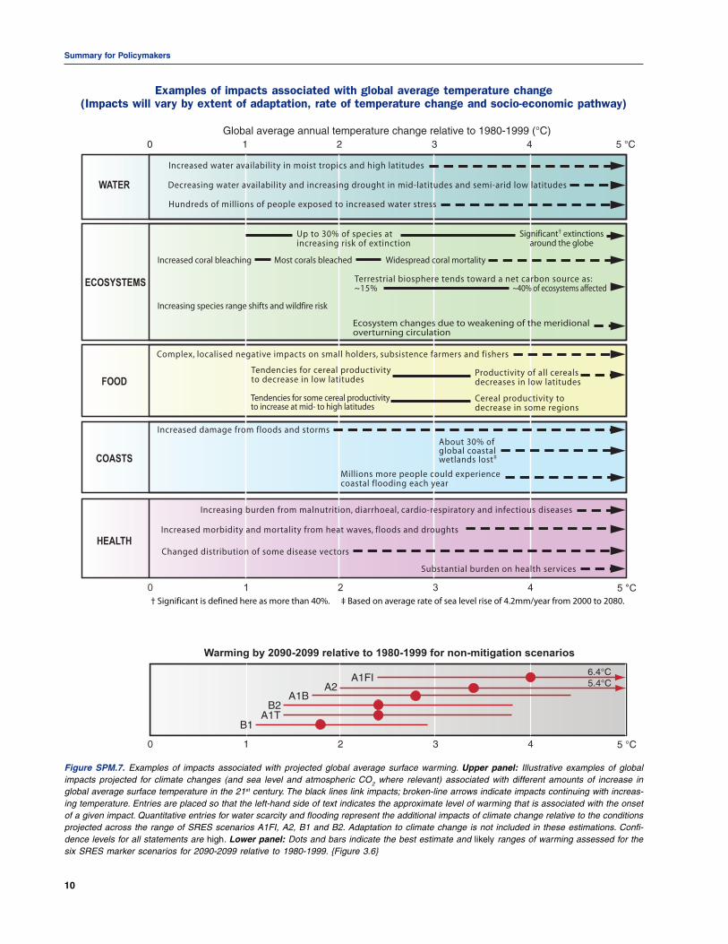
Studies since the TAR have enabled more systematicunderstanding of the timing and magnitude of impactsrelated to differing amounts and rates of climatechange. {3.3.1, 3.3.2}
Figure SPM.7 presents examples of this new informationfor systems and sectors. The top panel shows impacts increas-ing with increasing temperature change. Their estimated mag-nitude and timing is also affected by development pathway(lower panel). {3.3.1}
Examples of some projected impacts for different regionsare given in Table SPM.2.
Table SPM.1. Projected global average surface warming and sea level rise at the end of the 21st century. {Table 3.1}
Temperature change Sea level rise(°C at 2090-2099 relative to 1980-1999) a, d (m at 2090-2099 relative to 1980-1999)
Case Best estimate Likely range Model-based rangeexcluding future rapid dynamical changes in ice flow
Constant year 2000concentrationsb 0.6 0.3 – 0.9 Not available
B1 scenario 1.8 1.1 – 2.9 0.18 – 0.38A1T scenario 2.4 1.4 – 3.8 0.20 – 0.45B2 scenario 2.4 1.4 – 3.8 0.20 – 0.43A1B scenario 2.8 1.7 – 4.4 0.21 – 0.48A2 scenario 3.4 2.0 – 5.4 0.23 – 0.51A1FI scenario 4.0 2.4 – 6.4 0.26 – 0.59
Notes:a) Temperatures are assessed best estimates and likely uncertainty ranges from a hierarchy of models of varying complexity as well as
observational constraints.b) Year 2000 constant composition is derived from Atmosphere-Ocean General Circulation Models (AOGCMs) only.c) All scenarios above are six SRES marker scenarios. Approximate CO2-eq concentrations corresponding to the computed radiative
forcing due to anthropogenic GHGs and aerosols in 2100 (see p. 823 of the Working Group I TAR) for the SRES B1, AIT, B2, A1B, A2and A1FI illustrative marker scenarios are about 600, 700, 800, 850, 1250 and 1550ppm, respectively.
d) Temperature changes are expressed as the difference from the period 1980-1999. To express the change relative to the period 1850-1899 add 0.5°C.

9
Summary for Policymakers
Geographical pattern of surface warming
Figure SPM.6. Projected surface temperature changes for the late 21st century (2090-2099). The map shows the multi-AOGCM average projec-tion for the A1B SRES scenario. Temperatures are relative to the period 1980-1999. {Figure 3.2}
Some systems, sectors and regions are likely to be espe-cially affected by climate change.12 {3.3.3}
Systems and sectors: {3.3.3}
� particular ecosystems:- terrestrial: tundra, boreal forest and mountain regions
because of sensitivity to warming; mediterranean-typeecosystems because of reduction in rainfall; and tropi-cal rainforests where precipitation declines
- coastal: mangroves and salt marshes, due to multiplestresses
- marine: coral reefs due to multiple stresses; the sea icebiome because of sensitivity to warming
� water resources in some dry regions at mid-latitudes13 andin the dry tropics, due to changes in rainfall and evapo-transpiration, and in areas dependent on snow and ice melt
� agriculture in low latitudes, due to reduced water avail-ability
� low-lying coastal systems, due to threat of sea level riseand increased risk from extreme weather events
� human health in populations with low adaptive capacity.
Regions: {3.3.3}
� the Arctic, because of the impacts of high rates of projectedwarming on natural systems and human communities
� Africa, because of low adaptive capacity and projectedclimate change impacts
� small islands, where there is high exposure of populationand infrastructure to projected climate change impacts
� Asian and African megadeltas, due to large populationsand high exposure to sea level rise, storm surges and riverflooding.
Within other areas, even those with high incomes, somepeople (such as the poor, young children and the elderly) canbe particularly at risk, and also some areas and some activi-ties. {3.3.3}
Ocean acidification
The uptake of anthropogenic carbon since 1750 has led tothe ocean becoming more acidic with an average decrease inpH of 0.1 units. Increasing atmospheric CO
2 concentrations
lead to further acidification. Projections based on SRES sce-narios give a reduction in average global surface ocean pH ofbetween 0.14 and 0.35 units over the 21st century. While the ef-fects of observed ocean acidification on the marine biosphere areas yet undocumented, the progressive acidification of oceans isexpected to have negative impacts on marine shell-forming or-ganisms (e.g. corals) and their dependent species. {3.3.4}
12 Identified on the basis of expert judgement of the assessed literature and considering the magnitude, timing and projected rate of climatechange, sensitivity and adaptive capacity.13 Including arid and semi-arid regions.
Summary for Policymakers
10
Examples of impacts associated with global average temperature change
(Impacts will vary by extent of adaptation, rate of temperature change and socio-economic pathway)
Figure SPM.7. Examples of impacts associated with projected global average surface warming. Upper panel: Illustrative examples of globalimpacts projected for climate changes (and sea level and atmospheric CO2 where relevant) associated with different amounts of increase inglobal average surface temperature in the 21st century. The black lines link impacts; broken-line arrows indicate impacts continuing with increas-ing temperature. Entries are placed so that the left-hand side of text indicates the approximate level of warming that is associated with the onsetof a given impact. Quantitative entries for water scarcity and flooding represent the additional impacts of climate change relative to the conditionsprojected across the range of SRES scenarios A1FI, A2, B1 and B2. Adaptation to climate change is not included in these estimations. Confi-dence levels for all statements are high. Lower panel: Dots and bars indicate the best estimate and likely ranges of warming assessed for thesix SRES marker scenarios for 2090-2099 relative to 1980-1999. {Figure 3.6}
Warming by 2090-2099 relative to 1980-1999 for non-mitigation scenarios
6.4°C5.4°C
0 1 2 3 4 5 °CGlobal average annual temperature change relative to 1980-1999 (°C)
5 °C0 1 2 3 4
About 30% of global coastal wetlands lost‡
Increased water availability in moist tropics and high latitudes
Decreasing water availability and increasing drought in mid-latitudes and semi-arid low latitudes
Hundreds of millions of people exposed to increased water stress
Up to 30% of species at increasing risk of extinction
Increased coral bleaching Most corals bleached Widespread coral mortality
Increasing species range shifts and wildfire risk
Terrestrial biosphere tends toward a net carbon source as:~15% ~40% of ecosystems affected
Tendencies for cereal productivityto decrease in low latitudes
Productivity of all cereals decreases in low latitudes
Cereal productivity todecrease in some regions
Complex, localised negative impacts on small holders, subsistence farmers and fishers
Tendencies for some cereal productivity to increase at mid- to high latitudes
Significant† extinctions around the globe
Changed distribution of some disease vectors
Increasing burden from malnutrition, diarrhoeal, cardio-respiratory and infectious diseases
Increased morbidity and mortality from heat waves, floods and droughts
Substantial burden on health services
Ecosystem changes due to weakening of the meridional overturning circulation
Millions more people could experience coastal flooding each year
Increased damage from floods and storms
WATER
ECOSYSTEMS
FOOD
COASTS
HEALTH
5 °C0 1 2 3 4
† Significant is defined here as more than 40%. ‡ Based on average rate of sea level rise of 4.2mm/year from 2000 to 2080.

11
Summary for Policymakers
Table SPM.2. Examples of some projected regional impacts. {3.3.2}
Africa � By 2020, between 75 and 250 million of people are projected to be exposed to increased water stress due toclimate change.
� By 2020, in some countries, yields from rain-fed agriculture could be reduced by up to 50%. Agriculturalproduction, including access to food, in many African countries is projected to be severely compromised. Thiswould further adversely affect food security and exacerbate malnutrition.
� Towards the end of the 21st century, projected sea level rise will affect low-lying coastal areas with largepopulations. The cost of adaptation could amount to at least 5 to 10% of Gross Domestic Product (GDP).
� By 2080, an increase of 5 to 8% of arid and semi-arid land in Africa is projected under a range of climatescenarios (TS).
Asia � By the 2050s, freshwater availability in Central, South, East and South-East Asia, particularly in large riverbasins, is projected to decrease.
� Coastal areas, especially heavily populated megadelta regions in South, East and South-East Asia, will be atgreatest risk due to increased flooding from the sea and, in some megadeltas, flooding from the rivers.
� Climate change is projected to compound the pressures on natural resources and the environmentassociated with rapid urbanisation, industrialisation and economic development.
� Endemic morbidity and mortality due to diarrhoeal disease primarily associated with floods and droughtsare expected to rise in East, South and South-East Asia due to projected changes in the hydrological cycle.
Australia and � By 2020, significant loss of biodiversity is projected to occur in some ecologically rich sites, including theNew Zealand Great Barrier Reef and Queensland Wet Tropics.
� By 2030, water security problems are projected to intensify in southern and eastern Australia and, inNew Zealand, in Northland and some eastern regions.
� By 2030, production from agriculture and forestry is projected to decline over much of southern andeastern Australia, and over parts of eastern New Zealand, due to increased drought and fire. However, inNew Zealand, initial benefits are projected in some other regions.
� By 2050, ongoing coastal development and population growth in some areas of Australia and New Zealandare projected to exacerbate risks from sea level rise and increases in the severity and frequency of stormsand coastal flooding.
Europe � Climate change is expected to magnify regional differences in Europe’s natural resources and assets.Negative impacts will include increased risk of inland flash floods and more frequent coastal flooding andincreased erosion (due to storminess and sea level rise).
� Mountainous areas will face glacier retreat, reduced snow cover and winter tourism, and extensive specieslosses (in some areas up to 60% under high emissions scenarios by 2080).
� In southern Europe, climate change is projected to worsen conditions (high temperatures and drought) ina region already vulnerable to climate variability, and to reduce water availability, hydropower potential,summer tourism and, in general, crop productivity.
� Climate change is also projected to increase the health risks due to heat waves and the frequency of wildfires.
Latin America � By mid-century, increases in temperature and associated decreases in soil water are projected to lead togradual replacement of tropical forest by savanna in eastern Amazonia. Semi-arid vegetation will tend tobe replaced by arid-land vegetation.
� There is a risk of significant biodiversity loss through species extinction in many areas of tropical Latin America.� Productivity of some important crops is projected to decrease and livestock productivity to decline, with
adverse consequences for food security. In temperate zones, soybean yields are projected to increase.Overall, the number of people at risk of hunger is projected to increase (TS; medium confidence).
� Changes in precipitation patterns and the disappearance of glaciers are projected to significantly affectwater availability for human consumption, agriculture and energy generation.
North America � Warming in western mountains is projected to cause decreased snowpack, more winter flooding andreduced summer flows, exacerbating competition for over-allocated water resources.
� In the early decades of the century, moderate climate change is projected to increase aggregate yields ofrain-fed agriculture by 5 to 20%, but with important variability among regions. Major challenges areprojected for crops that are near the warm end of their suitable range or which depend on highly utilisedwater resources.
� Cities that currently experience heat waves are expected to be further challenged by an increasednumber, intensity and duration of heat waves during the course of the century, with potential for adversehealth impacts.
� Coastal communities and habitats will be increasingly stressed by climate change impacts interactingwith development and pollution.
continued...

Summary for Policymakers
12
Altered frequencies and intensities of extreme weather,together with sea level rise, are expected to have mostlyadverse effects on natural and human systems. {3.3.5}
Examples for selected extremes and sectors are shown inTable SPM.3.
Anthropogenic warming and sea level rise would con-tinue for centuries due to the time scales associatedwith climate processes and feedbacks, even if GHGconcentrations were to be stabilised. {3.2.3}
Estimated long-term (multi-century) warming correspond-ing to the six AR4 Working Group III stabilisation categoriesis shown in Figure SPM.8.
Contraction of the Greenland ice sheet is projected to con-tinue to contribute to sea level rise after 2100. Current modelssuggest virtually complete elimination of the Greenland icesheet and a resulting contribution to sea level rise of about 7mif global average warming were sustained for millennia inexcess of 1.9 to 4.6°C relative to pre-industrial values. Thecorresponding future temperatures in Greenland are compa-rable to those inferred for the last interglacial period 125,000years ago, when palaeoclimatic information suggests reductionsof polar land ice extent and 4 to 6m of sea level rise. {3.2.3}
Current global model studies project that the Antarctic icesheet will remain too cold for widespread surface melting andgain mass due to increased snowfall. However, net loss of icemass could occur if dynamical ice discharge dominates theice sheet mass balance. {3.2.3}
Table SPM.2. continued...
Polar Regions � The main projected biophysical effects are reductions in thickness and extent of glaciers, ice sheetsand sea ice, and changes in natural ecosystems with detrimental effects on many organisms includingmigratory birds, mammals and higher predators.
� For human communities in the Arctic, impacts, particularly those resulting from changing snow and iceconditions, are projected to be mixed.
� Detrimental impacts would include those on infrastructure and traditional indigenous ways of life.� In both polar regions, specific ecosystems and habitats are projected to be vulnerable, as climatic barriers to
species invasions are lowered.
Small Islands � Sea level rise is expected to exacerbate inundation, storm surge, erosion and other coastal hazards, thusthreatening vital infrastructure, settlements and facilities that support the livelihood of island communities.
� Deterioration in coastal conditions, for example through erosion of beaches and coral bleaching, is expectedto affect local resources.
� By mid-century, climate change is expected to reduce water resources in many small islands, e.g. inthe Caribbean and Pacific, to the point where they become insufficient to meet demand during low-rainfallperiods.
� With higher temperatures, increased invasion by non-native species is expected to occur, particularly onmid- and high-latitude islands.
Note:Unless stated explicitly, all entries are from Working Group II SPM text, and are either very high confidence or high confidence state-ments, reflecting different sectors (agriculture, ecosystems, water, coasts, health, industry and settlements). The Working Group II SPMrefers to the source of the statements, timelines and temperatures. The magnitude and timing of impacts that will ultimately be realisedwill vary with the amount and rate of climate change, emissions scenarios, development pathways and adaptation.
Figure SPM.8. Estimated long-term (multi-century) warming corresponding to the six AR4 Working Group III stabilisation categories (TableSPM.6). The temperature scale has been shifted by -0.5°C compared to Table SPM.6 to account approximately for the warming between pre-industrial and 1980-1999. For most stabilisation levels global average temperature is approaching the equilibrium level over a few centuries. ForGHG emissions scenarios that lead to stabilisation at levels comparable to SRES B1 and A1B by 2100 (600 and 850ppm CO2-eq; category IVand V), assessed models project that about 65 to 70% of the estimated global equilibrium temperature increase, assuming a climate sensitivityof 3°C, would be realised at the time of stabilisation. For the much lower stabilisation scenarios (category I and II, Figure SPM.11), the equilib-rium temperature may be reached earlier. {Figure 3.4}
Estimated multi-century warming relative to 1980-1999 for AR4 stabilisation categories
0 1 2 3 4 5 6 °CGlobal average temperature change relative to 1980-1999 (°C)

13
Summary for Policymakers
Table SPM.3. Examples of possible impacts of climate change due to changes in extreme weather and climate events, based onprojections to the mid- to late 21st century. These do not take into account any changes or developments in adaptive capacity. Thelikelihood estimates in column two relate to the phenomena listed in column one. {Table 3.2}
Anthropogenic warming could lead to some impactsthat are abrupt or irreversible, depending upon the rateand magnitude of the climate change. {3.4}
Partial loss of ice sheets on polar land could imply metresof sea level rise, major changes in coastlines and inundationof low-lying areas, with greatest effects in river deltas andlow-lying islands. Such changes are projected to occur over
millennial time scales, but more rapid sea level rise on cen-tury time scales cannot be excluded. {3.4}
Climate change is likely to lead to some irreversible im-pacts. There is medium confidence that approximately 20 to30% of species assessed so far are likely to be at increasedrisk of extinction if increases in global average warming ex-ceed 1.5 to 2.5°C (relative to 1980-1999). As global average
Phenomenona and Likelihood of Examples of major projected impacts by sectordirection of trend future trends
based on Agriculture, forestry Water resources Human health Industry, settlementprojections and ecosystems and societyfor 21st centuryusing SRESscenarios
Over most land Virtually Increased yields in Effects on water Reduced human Reduced energy demand forareas, warmer and certainb colder environments; resources relying on mortality from heating; increased demandfewer cold days decreased yields in snowmelt; effects on decreased cold for cooling; declining air qualityand nights, warmer warmer environments; some water supplies exposure in cities; reduced disruption toand more frequent increased insect transport due to snow, ice;hot days and nights outbreaks effects on winter tourism
Warm spells/heat Very likely Reduced yields in Increased water Increased risk of Reduction in quality of life forwaves. Frequency warmer regions demand; water heat-related people in warm areas withoutincreases over most due to heat stress; quality problems, mortality, especially appropriate housing; impactsland areas increased danger of e.g. algal blooms for the elderly, on the elderly, very young and
wildfire chronically sick, poorvery young andsocially isolated
Heavy precipitation Very likely Damage to crops; Adverse effects on Increased risk of Disruption of settlements,events. Frequency soil erosion, inability quality of surface deaths, injuries and commerce, transport andincreases over most to cultivate land due and groundwater; infectious, respiratory societies due to flooding:areas to waterlogging of contamination of and skin diseases pressures on urban and rural
soils water supply; water infrastructures; loss of propertyscarcity may berelieved
Area affected by Likely Land degradation; More widespread Increased risk of Water shortage for settlements,drought increases lower yields/crop water stress food and water industry and societies;
damage and failure; shortage; increased reduced hydropower generationincreased livestock risk of malnutrition; potentials; potential fordeaths; increased increased risk of population migrationrisk of wildfire water- and food-
borne diseases
Intense tropical Likely Damage to crops; Power outages Increased risk of Disruption by flood and highcyclone activity windthrow (uprooting) causing disruption deaths, injuries, winds; withdrawal of riskincreases of trees; damage to of public water supply water- and food- coverage in vulnerable areas
coral reefs borne diseases; by private insurers; potentialpost-traumatic for population migrations; lossstress disorders of property
Increased incidence Likely d Salinisation of Decreased fresh- Increased risk of Costs of coastal protectionof extreme high irrigation water, water availability due deaths and injuries versus costs of land-usesea level (excludes estuaries and fresh- to saltwater intrusion by drowning in floods; relocation; potential fortsunamis)c water systems migration-related movement of populations and
health effects infrastructure; also see tropicalcyclones above
Notes:a) See Working Group I Table 3.7 for further details regarding definitions.b) Warming of the most extreme days and nights each year.c) Extreme high sea level depends on average sea level and on regional weather systems. It is defined as the highest 1% of hourly values
of observed sea level at a station for a given reference period.d) In all scenarios, the projected global average sea level at 2100 is higher than in the reference period. The effect of changes in regional
weather systems on sea level extremes has not been assessed.

Summary for Policymakers
14
temperature increase exceeds about 3.5°C, model projectionssuggest significant extinctions (40 to 70% of species assessed)around the globe. {3.4}
Based on current model simulations, the meridional over-turning circulation (MOC) of the Atlantic Ocean will very likelyslow down during the 21st century; nevertheless temperaturesover the Atlantic and Europe are projected to increase. TheMOC is very unlikely to undergo a large abrupt transition dur-ing the 21st century. Longer-term MOC changes cannot be as-sessed with confidence. Impacts of large-scale and persistentchanges in the MOC are likely to include changes in marineecosystem productivity, fisheries, ocean CO
2 uptake, oceanic
oxygen concentrations and terrestrial vegetation. Changes interrestrial and ocean CO
2 uptake may feed back on the cli-
mate system. {3.4}
4. Adaptation and mitigation options14
A wide array of adaptation options is available, but moreextensive adaptation than is currently occurring is re-quired to reduce vulnerability to climate change. Thereare barriers, limits and costs, which are not fully un-derstood. {4.2}
Societies have a long record of managing the impacts ofweather- and climate-related events. Nevertheless, additionaladaptation measures will be required to reduce the adverseimpacts of projected climate change and variability, regard-less of the scale of mitigation undertaken over the next two tothree decades. Moreover, vulnerability to climate change canbe exacerbated by other stresses. These arise from, for ex-ample, current climate hazards, poverty and unequal access toresources, food insecurity, trends in economic globalisation,conflict and incidence of diseases such as HIV/AIDS. {4.2}
Some planned adaptation to climate change is alreadyoccurring on a limited basis. Adaptation can reduce vulner-
ability, especially when it is embedded within broader sectoralinitiatives (Table SPM.4). There is high confidence that thereare viable adaptation options that can be implemented in somesectors at low cost, and/or with high benefit-cost ratios. How-ever, comprehensive estimates of global costs and benefits ofadaptation are limited. {4.2, Table 4.1}
Adaptive capacity is intimately connected to social andeconomic development but is unevenly distributedacross and within societies. {4.2}
A range of barriers limits both the implementation andeffectiveness of adaptation measures. The capacity to adapt isdynamic and is influenced by a society’s productive base, in-cluding natural and man-made capital assets, social networksand entitlements, human capital and institutions, governance,national income, health and technology. Even societies withhigh adaptive capacity remain vulnerable to climate change,variability and extremes. {4.2}
Both bottom-up and top-down studies indicate thatthere is high agreement and much evidence of sub-stantial economic potential for the mitigation of globalGHG emissions over the coming decades that couldoffset the projected growth of global emissions or re-duce emissions below current levels (Figures SPM.9,SPM.10).15 While top-down and bottom-up studies arein line at the global level (Figure SPM.9) there are con-siderable differences at the sectoral level. {4.3}
No single technology can provide all of the mitigationpotential in any sector. The economic mitigation potential,which is generally greater than the market mitigation poten-tial, can only be achieved when adequate policies are in placeand barriers removed (Table SPM.5). {4.3}
Bottom-up studies suggest that mitigation opportunitieswith net negative costs have the potential to reduce emissionsby around 6 GtCO
2-eq/yr in 2030, realising which requires
dealing with implementation barriers. {4.3}
14 While this Section deals with adaptation and mitigation separately, these responses can be complementary. This theme is discussed inSection 5.15 The concept of ‘mitigation potential’ has been developed to assess the scale of GHG reductions that could be made, relative to emissionbaselines, for a given level of carbon price (expressed in cost per unit of carbon dioxide equivalent emissions avoided or reduced). Mitigationpotential is further differentiated in terms of ‘market mitigation potential’ and ‘economic mitigation potential’.
Market mitigation potential is the mitigation potential based on private costs and private discount rates (reflecting the perspective of privateconsumers and companies), which might be expected to occur under forecast market conditions, including policies and measures currently inplace, noting that barriers limit actual uptake.
Economic mitigation potential is the mitigation potential that takes into account social costs and benefits and social discount rates (reflect-ing the perspective of society; social discount rates are lower than those used by private investors), assuming that market efficiency isimproved by policies and measures and barriers are removed.
Mitigation potential is estimated using different types of approaches. Bottom-up studies are based on assessment of mitigation options,emphasising specific technologies and regulations. They are typically sectoral studies taking the macro-economy as unchanged. Top-downstudies assess the economy-wide potential of mitigation options. They use globally consistent frameworks and aggregated information aboutmitigation options and capture macro-economic and market feedbacks.

15
Summary for Policymakers
Table SPM.4. Selected examples of planned adaptation by sector. {Table 4.1}
Adaptation option/strategy
Expanded rainwater harvesting;water storage and conservationtechniques; water re-use;desalination; water-use andirrigation efficiency
Adjustment of planting dates andcrop variety; crop relocation;improved land management, e.g.erosion control and soil protectionthrough tree planting
Relocation; seawalls and stormsurge barriers; dune reinforce-ment; land acquisition andcreation of marshlands/wetlandsas buffer against sea level riseand flooding; protection of existingnatural barriers
Heat-health action plans;emergency medical services;improved climate-sensitivedisease surveillance and control;safe water and improvedsanitation
Diversification of tourismattractions and revenues; shiftingski slopes to higher altitudes andglaciers; artificial snow-making
Ralignment/relocation; designstandards and planning for roads,rail and other infrastructure tocope with warming and drainage
Strengthening of overheadtransmission and distributioninfrastructure; undergroundcabling for utilities; energyefficiency; use of renewablesources; reduced dependence onsingle sources of energy
Underlying policy framework
National water policies andintegrated water resources manage-ment; water-related hazardsmanagement
R&D policies; institutional reform;land tenure and land reform; training;capacity building; crop insurance;financial incentives, e.g. subsidiesand tax credits
Standards and regulations thatintegrate climate change consider-ations into design; land-use policies;building codes; insurance
Public health policies that recogniseclimate risk; strengthened healthservices; regional and internationalcooperation
Integrated planning (e.g. carryingcapacity; linkages with othersectors); financial incentives, e.g.subsidies and tax credits
Integrating climate change consider-ations into national transport policy;investment in R&D for specialsituations, e.g. permafrost areas
National energy policies, regulations,and fiscal and financial incentives toencourage use of alternativesources; incorporating climatechange in design standards
Key constraints and opportunitiesto implementation (Normal font =constraints; italics = opportunities)
Financial, human resources andphysical barriers; integrated waterresources management; synergies withother sectors
Technological and financialconstraints; access to new varieties;markets; longer growing season inhigher latitudes; revenues from ‘new’products
Financial and technological barriers;availability of relocation space;integrated policies and management;synergies with sustainable developmentgoals
Limits to human tolerance (vulnerablegroups); knowledge limitations; financialcapacity; upgraded health services;improved quality of life
Appeal/marketing of new attractions;financial and logistical challenges;potential adverse impact on othersectors (e.g. artificial snow-making mayincrease energy use); revenues from‘new’ attractions; involvement of widergroup of stakeholders
Financial and technological barriers;availability of less vulnerable routes;improved technologies and integrationwith key sectors (e.g. energy)
Access to viable alternatives; financialand technological barriers; acceptanceof new technologies; stimulation of newtechnologies; use of local resources
Note:Other examples from many sectors would include early warning systems.
Future energy infrastructure investment decisions, ex-pected to exceed US$20 trillion16 between 2005 and 2030,will have long-term impacts on GHG emissions, because ofthe long lifetimes of energy plants and other infrastructurecapital stock. The widespread diffusion of low-carbon tech-nologies may take many decades, even if early investments in
these technologies are made attractive. Initial estimates showthat returning global energy-related CO
2 emissions to 2005
levels by 2030 would require a large shift in investment pat-terns, although the net additional investment required rangesfrom negligible to 5 to 10%. {4.3}
Sector
Water
Agriculture
Infrastructure/settlement(includingcoastal zones)
Human health
Tourism
Transport
Energy
16 20 trillion = 20,000 billion = 20×1012

Summary for Policymakers
16
Figure SPM.10. Estimated economic mitigation potential by sector in 2030 from bottom-up studies, compared to the respective baselinesassumed in the sector assessments. The potentials do not include non-technical options such as lifestyle changes. {Figure 4.2}
Notes:a) The ranges for global economic potentials as assessed in each sector are shown by vertical lines. The ranges are based on end-use allocations of
emissions, meaning that emissions of electricity use are counted towards the end-use sectors and not to the energy supply sector.b) The estimated potentials have been constrained by the availability of studies particularly at high carbon price levels.c) Sectors used different baselines. For industry, the SRES B2 baseline was taken, for energy supply and transport, the World Energy Outlook
(WEO) 2004 baseline was used; the building sector is based on a baseline in between SRES B2 and A1B; for waste, SRES A1B drivingforces were used to construct a waste-specific baseline; agriculture and forestry used baselines that mostly used B2 driving forces.
d) Only global totals for transport are shown because international aviation is included.e) Categories excluded are: non-CO2 emissions in buildings and transport, part of material efficiency options, heat production and co-genera-
tion in energy supply, heavy duty vehicles, shipping and high-occupancy passenger transport, most high-cost options for buildings, wastewa-ter treatment, emission reduction from coal mines and gas pipelines, and fluorinated gases from energy supply and transport. The underes-timation of the total economic potential from these emissions is of the order of 10 to 15%.
Economic mitigation potentials by sector in 2030 estimated from bottom-up studies
2.4-4.7 1.6-2.5 5.3-6.7 2.5-5.5 2.3-6.4 1.3-4.2 0.4-1.0total sectoral potential at <US$100/tCO -eq in GtCO -eq/yr:2 2
Energy supply Transport Buildings Industry Agriculture Forestry Waste
World total
Figure SPM.9. Global economic mitigation potential in 2030 estimated from bottom-up (Panel a) and top-down (Panel b) studies, compared withthe projected emissions increases from SRES scenarios relative to year 2000 GHG emissions of 40.8 GtCO2-eq (Panel c). Note: GHG emissionsin 2000 are exclusive of emissions of decay of above ground biomass that remains after logging and deforestation and from peat fires anddrained peat soils, to ensure consistency with the SRES emission results. {Figure 4.1}
Comparison between global economic mitigation potential and projected emissions increase in 2030
0
5
10
15
20
25
30
35
A1FI A2 A1B A1T B1B2
Gt CO2-eq
c)< 0 < 20 < 50 < 100 US$/tCO2-eq
low end of range high end of range0
5
10
15
20
25
30
35
a)
low end of range high end of range0
5
10
15
20
25
30
35
< 20 < 50 < 100 US$/tCO2-eqb) Increase in GHG emissions
above year 2000 levelsBottom-up Top-down
Gt CO2-eq Gt CO2-eq
Est
imat
ed m
itiga
tion
pote
ntia
l in
2030
Est
imat
ed m
itiga
tion
pote
ntia
l in
2030

17
Summary for Policymakers
Tab
le S
PM
.5
Sel
ecte
d ex
ampl
es o
f ke
y se
ctor
al m
itiga
tion
tech
nolo
gies
, po
licie
s an
d m
easu
res,
con
stra
ints
and
opp
ortu
nitie
s. {
Tabl
e 4.
2}
Key
mit
igat
ion
tec
hn
olo
gie
s an
d p
ract
ices
cu
rren
tly
com
mer
cial
ly a
vaila
ble
.K
ey m
itig
atio
n t
ech
no
log
ies
and
pra
ctic
es p
roje
cted
to
be
com
mer
cial
ised
bef
ore
203
0 sh
ow
n in
ital
ics.
Impr
oved
sup
ply
and
dist
ribu
tion
effic
ienc
y; f
uel s
witc
hing
fro
m c
oal t
o ga
s; n
ucle
arpo
wer
; ren
ewab
le h
eat
and
pow
er (
hydr
opow
er,
sola
r, w
ind,
geo
ther
mal
and
bioe
nerg
y); c
ombi
ned
heat
and
pow
er; e
arly
app
licat
ions
of
carb
on d
ioxi
de c
aptu
rean
d st
orag
e (C
CS
) (e
.g. s
tora
ge o
f re
mov
ed C
O2
from
nat
ural
gas
); C
CS
for
gas,
biom
ass
and
coal
-fire
d el
ectr
icity
gen
erat
ing
faci
litie
s; a
dvan
ced
nucl
ear
pow
er;
adva
nced
ren
ewab
le e
nerg
y, in
clud
ing
tidal
and
wav
e en
ergy
, co
ncen
trat
ing
sola
r,an
d so
lar
phot
ovol
taic
s
Mor
e fu
el-e
ffici
ent
vehi
cles
; hy
brid
veh
icle
s; c
lean
er d
iese
l veh
icle
s; b
iofu
els;
mod
alsh
ifts
from
roa
d tr
ansp
ort
to r
ail a
nd p
ublic
tra
nspo
rt s
yste
ms;
non
-mot
oris
edtr
ansp
ort
(cyc
ling,
wal
king
); la
nd-u
se a
nd t
rans
port
pla
nnin
g; s
econ
d ge
nera
tion
biof
uels
; hig
her
effic
ienc
y ai
rcra
ft; a
dvan
ced
elec
tric
and
hyb
rid
vehi
cles
with
mor
epo
wer
ful a
nd r
elia
ble
batte
ries
Effi
cien
t lig
htin
g an
d da
ylig
htin
g; m
ore
effic
ient
ele
ctri
cal a
pplia
nces
and
hea
ting
and
cool
ing
devi
ces;
impr
oved
coo
k st
oves
, im
prov
ed in
sula
tion;
pas
sive
and
act
ive
sola
r de
sign
for
heat
ing
and
cool
ing;
alte
rnat
ive
refr
iger
atio
n flu
ids,
rec
over
y an
dre
cycl
ing
of f
luor
inat
ed g
ases
; in
tegr
ated
des
ign
of c
omm
erci
al b
uild
ings
incl
udin
gte
chno
logi
es,
such
as
inte
llige
nt m
eter
s th
at p
rovi
de f
eedb
ack
and
cont
rol;
sola
rph
otov
olta
ics
inte
grat
ed in
bui
ldin
gs
Mor
e ef
ficie
nt e
nd-u
se e
lect
rica
l equ
ipm
ent;
heat
and
pow
er r
ecov
ery;
mat
eria
lre
cycl
ing
and
subs
titut
ion;
con
trol
of
non-
CO
2 ga
s em
issi
ons;
and
a w
ide
arra
y of
proc
ess-
spec
ific
tech
nolo
gies
; ad
vanc
ed e
nerg
y ef
ficie
ncy;
CC
S f
or c
emen
t,am
mon
ia,
and
iron
man
ufac
ture
; ine
rt e
lect
rode
s fo
r al
umin
ium
man
ufac
ture
Impr
oved
cro
p an
d gr
azin
g la
nd m
anag
emen
t to
incr
ease
soi
l car
bon
stor
age;
rest
orat
ion
of c
ultiv
ated
pea
ty s
oils
and
deg
rade
d la
nds;
impr
oved
ric
e cu
ltiva
tion
tech
niqu
es a
nd li
vest
ock
and
man
ure
man
agem
ent
to r
educ
e C
H4
emis
sion
s;im
prov
ed n
itrog
en f
ertil
iser
app
licat
ion
tech
niqu
es t
o re
duce
N2O
em
issi
ons;
dedi
cate
d en
ergy
cro
ps t
o re
plac
e fo
ssil
fuel
use
; im
prov
ed e
nerg
y ef
ficie
ncy;
impr
ovem
ents
of
crop
yie
lds
Affo
rest
atio
n; r
efor
esta
tion;
for
est
man
agem
ent;
redu
ced
defo
rest
atio
n; h
arve
sted
woo
d pr
oduc
t m
anag
emen
t; us
e of
for
estr
y pr
oduc
ts f
or b
ioen
ergy
to
repl
ace
foss
ilfu
el u
se; t
ree
spec
ies
impr
ovem
ent
to in
crea
se b
iom
ass
prod
uctiv
ity a
nd c
arbo
nse
ques
trat
ion;
impr
oved
rem
ote
sens
ing
tech
nolo
gies
for
ana
lysi
s of
veg
etat
ion/
soil
carb
on s
eque
stra
tion
pote
ntia
l and
map
ping
land
-use
cha
nge
Land
fill C
H4
reco
very
; was
te in
cine
ratio
n w
ith e
nerg
y re
cove
ry;
com
post
ing
ofor
gani
c w
aste
; co
ntro
lled
was
tew
ater
tre
atm
ent;
recy
clin
g an
d w
aste
min
imis
atio
n;bi
ocov
ers
and
biof
ilter
s to
opt
imis
e C
H4
oxid
atio
n
Po
licie
s, m
easu
res
and
in
stru
men
ts s
how
n t
o b
een
viro
nm
enta
lly e
ffec
tive
Red
uctio
n of
fos
sil f
uel s
ubsi
dies
; ta
xes
or c
arbo
n ch
arge
son
fos
sil f
uels
Fee
d-in
tar
iffs
for
rene
wab
le e
nerg
y te
chno
logi
es;
rene
wab
le e
nerg
y ob
ligat
ions
; pr
oduc
er s
ubsi
dies
Man
dato
ry f
uel e
cono
my;
bio
fuel
ble
ndin
g an
d C
O2
stan
dard
s fo
r ro
ad t
rans
port
Taxe
s on
veh
icle
pur
chas
e, r
egis
trat
ion,
use
and
mot
orfu
els;
roa
d an
d pa
rkin
g pr
icin
g
Influ
ence
mob
ility
nee
ds t
hrou
gh la
nd-u
se r
egul
atio
ns a
ndin
fras
truc
ture
pla
nnin
g; in
vest
men
t in
attr
activ
e pu
blic
tran
spor
t fa
cilit
ies
and
non-
mot
oris
ed f
orm
s of
tra
nspo
rt
App
lianc
e st
anda
rds
and
labe
lling
Bui
ldin
g co
des
and
cert
ifica
tion
Dem
and-
side
man
agem
ent
prog
ram
mes
Pub
lic s
ecto
r le
ader
ship
pro
gram
mes
, in
clud
ing
proc
urem
ent
Ince
ntiv
es f
or e
nerg
y se
rvic
e co
mpa
nies
(E
SC
Os)
Pro
visi
on o
f be
nchm
ark
info
rmat
ion;
per
form
ance
stan
dard
s; s
ubsi
dies
; ta
x cr
edits
Trad
able
per
mits
Vol
unta
ry a
gree
men
ts
Fin
anci
al in
cent
ives
and
reg
ulat
ions
for
impr
oved
land
man
agem
ent;
mai
ntai
ning
soi
l car
bon
cont
ent;
effic
ient
use
of f
ertil
iser
s an
d irr
igat
ion
Fin
anci
al in
cent
ives
(na
tiona
l and
inte
rnat
iona
l) to
incr
ease
for
est
area
, to
red
uce
defo
rest
atio
n an
d to
mai
ntai
n an
d m
anag
e fo
rest
s; la
nd-u
se r
egul
atio
n an
den
forc
emen
t
Fin
anci
al in
cent
ives
for
impr
oved
was
te a
nd w
aste
wat
erm
anag
emen
t
Ren
ewab
le e
nerg
y in
cent
ives
or
oblig
atio
ns
Was
te m
anag
emen
t re
gula
tions
Key
co
nst
rain
ts o
r o
pp
ort
un
itie
s(N
orm
al fo
nt =
con
stra
ints
;ita
lics
= op
port
uniti
es)
Res
ista
nce
by v
este
d in
tere
sts
may
mak
e th
emdi
fficu
lt to
impl
emen
t
May
be
appr
opria
te t
o cr
eate
mar
kets
for
low
-em
issi
ons
tech
nolo
gies
Par
tial c
over
age
of v
ehic
le f
leet
may
lim
itef
fect
iven
ess
Effe
ctiv
enes
s m
ay d
rop
with
hig
her
inco
mes
Par
ticul
arly
app
ropr
iate
for
cou
ntrie
s th
at a
rebu
ildin
g up
the
ir tr
ansp
orta
tion
syst
ems
Per
iodi
c re
visi
on o
f st
anda
rds
need
ed
Attr
activ
e fo
r ne
w b
uild
ings
. E
nfor
cem
ent
can
bedi
ffic
ult
Nee
d fo
r re
gula
tions
so
that
util
ities
may
pro
fit
Gov
ernm
ent
purc
hasi
ng c
an e
xpan
d de
man
d fo
ren
ergy
-effi
cien
t pr
oduc
ts
Suc
cess
fact
or: A
cces
s to
thi
rd p
arty
fin
anci
ng
May
be
appr
opri
ate
to s
timul
ate
tech
nolo
gy u
ptak
e.S
tabi
lity
of n
atio
nal p
olic
y im
port
ant
in v
iew
of
inte
rnat
iona
l co
mpe
titiv
enes
s
Pre
dict
able
allo
catio
n m
echa
nism
s an
d st
able
pric
e si
gnal
s im
port
ant
for
inve
stm
ents
Suc
cess
fac
tors
incl
ude:
cle
ar t
arge
ts,
a ba
selin
esc
enar
io,
third
-par
ty in
volv
emen
t in
des
ign
and
revi
ew a
nd fo
rmal
pro
visi
ons
of m
onito
ring
, cl
ose
coop
erat
ion
betw
een
gove
rnm
ent
and
indu
stry
May
enc
oura
ge s
yner
gy w
ith s
usta
inab
lede
velo
pmen
t an
d w
ith r
educ
ing
vuln
erab
ility
to
clim
ate
chan
ge,
ther
eby
over
com
ing
barr
iers
to
impl
emen
tatio
n
Con
stra
ints
incl
ude
lack
of
inve
stm
ent
capi
tal a
ndla
nd t
enur
e is
sues
. Can
hel
p po
vert
y al
levi
atio
n
May
stim
ulat
e te
chno
logy
diff
usio
n
Loca
l ava
ilabi
lity
of lo
w-c
ost
fuel
Mos
t ef
fect
ivel
y ap
plie
d at
nat
iona
l lev
el w
ithen
forc
emen
t st
rate
gies
Sec
tor
Ene
rgy
supp
ly
Tran
spo
rt
Bu
ildin
gs
Ind
ust
ry
Ag
ricu
ltu
re
Fo
rest
ry/
fore
sts
Was
te

Summary for Policymakers
18
A wide variety of policies and instruments are avail-able to governments to create the incentives for miti-gation action. Their applicability depends on nationalcircumstances and sectoral context (Table SPM.5). {4.3}
They include integrating climate policies in wider devel-opment policies, regulations and standards, taxes and charges,tradable permits, financial incentives, voluntary agreements,information instruments, and research, development and dem-onstration (RD&D). {4.3}
An effective carbon-price signal could realise significantmitigation potential in all sectors. Modelling studies show thatglobal carbon prices rising to US$20-80/tCO
2-eq by 2030 are
consistent with stabilisation at around 550ppm CO2-eq by 2100.
For the same stabilisation level, induced technological changemay lower these price ranges to US$5-65/tCO
2-eq in 2030.17 {4.3}
There is high agreement and much evidence that mitiga-tion actions can result in near-term co-benefits (e.g. improvedhealth due to reduced air pollution) that may offset a substan-tial fraction of mitigation costs. {4.3}
There is high agreement and medium evidence that AnnexI countries’ actions may affect the global economy and globalemissions, although the scale of carbon leakage remains un-certain.18 {4.3}
Fossil fuel exporting nations (in both Annex I and non-An-nex I countries) may expect, as indicated in the TAR, lower de-mand and prices and lower GDP growth due to mitigation poli-cies. The extent of this spillover depends strongly on assump-tions related to policy decisions and oil market conditions. {4.3}
There is also high agreement and medium evidence thatchanges in lifestyle, behaviour patterns and management prac-tices can contribute to climate change mitigation across all sec-tors. {4.3}
Many options for reducing global GHG emissionsthrough international cooperation exist. There is highagreement and much evidence that notable achieve-ments of the UNFCCC and its Kyoto Protocol are theestablishment of a global response to climate change,stimulation of an array of national policies, and the cre-ation of an international carbon market and new insti-tutional mechanisms that may provide the foundation
for future mitigation efforts. Progress has also been madein addressing adaptation within the UNFCCC and addi-tional international initiatives have been suggested. {4.5}
Greater cooperative efforts and expansion of market mecha-nisms will help to reduce global costs for achieving a given levelof mitigation, or will improve environmental effectiveness. Ef-forts can include diverse elements such as emissions targets;sectoral, local, sub-national and regional actions; RD&Dprogrammes; adopting common policies; implementing devel-opment-oriented actions; or expanding financing instruments. {4.5}
In several sectors, climate response options can beimplemented to realise synergies and avoid conflictswith other dimensions of sustainable development.Decisions about macroeconomic and other non-climatepolicies can significantly affect emissions, adaptivecapacity and vulnerability. {4.4, 5.8}
Making development more sustainable can enhance miti-gative and adaptive capacities, reduce emissions and reducevulnerability, but there may be barriers to implementation. Onthe other hand, it is very likely that climate change can slowthe pace of progress towards sustainable development. Overthe next half-century, climate change could impede achieve-ment of the Millennium Development Goals. {5.8}
5. The long-term perspective
Determining what constitutes “dangerous anthropo-genic interference with the climate system” in relationto Article 2 of the UNFCCC involves value judgements.Science can support informed decisions on this issue,including by providing criteria for judging which vul-nerabilities might be labelled ‘key’. {Box ‘Key Vulnerabili-ties and Article 2 of the UNFCCC’, Topic 5}
Key vulnerabilities19 may be associated with many cli-mate-sensitive systems, including food supply, infrastructure,health, water resources, coastal systems, ecosystems, globalbiogeochemical cycles, ice sheets and modes of oceanic andatmospheric circulation. {Box ‘Key Vulnerabilities and Article 2 of
the UNFCCC’, Topic 5}
17 Studies on mitigation portfolios and macro-economic costs assessed in this report are based on top-down modelling. Most models use aglobal least-cost approach to mitigation portfolios, with universal emissions trading, assuming transparent markets, no transaction cost, andthus perfect implementation of mitigation measures throughout the 21st century. Costs are given for a specific point in time. Global modelledcosts will increase if some regions, sectors (e.g. land use), options or gases are excluded. Global modelled costs will decrease with lowerbaselines, use of revenues from carbon taxes and auctioned permits, and if induced technological learning is included. These models do not considerclimate benefits and generally also co-benefits of mitigation measures, or equity issues. Significant progress has been achieved in applying ap-proaches based on induced technological change to stabilisation studies; however, conceptual issues remain. In the models that consider inducedtechnological change, projected costs for a given stabilisation level are reduced; the reductions are greater at lower stabilisation level.18 Further details may be found in Topic 4 of this Synthesis Report.19 Key vulnerabilities can be identified based on a number of criteria in the literature, including magnitude, timing, persistence/reversibility, thepotential for adaptation, distributional aspects, likelihood and ‘importance’ of the impacts.

19
Summary for Policymakers
The five ‘reasons for concern’ identified in the TAR re-main a viable framework to consider key vulnerabili-ties. These ‘reasons’ are assessed here to be strongerthan in the TAR. Many risks are identified with higher con-fidence. Some risks are projected to be larger or to occurat lower increases in temperature. Understanding aboutthe relationship between impacts (the basis for ‘reasonsfor concern’ in the TAR) and vulnerability (that includesthe ability to adapt to impacts) has improved. {5.2}
This is due to more precise identification of the circum-stances that make systems, sectors and regions especially vul-nerable and growing evidence of the risks of very large im-pacts on multiple-century time scales. {5.2}
� Risks to unique and threatened systems. There is newand stronger evidence of observed impacts of climatechange on unique and vulnerable systems (such as polarand high mountain communities and ecosystems), withincreasing levels of adverse impacts as temperatures in-crease further. An increasing risk of species extinction andcoral reef damage is projected with higher confidence thanin the TAR as warming proceeds. There is medium confi-dence that approximately 20 to 30% of plant and animalspecies assessed so far are likely to be at increased risk ofextinction if increases in global average temperature ex-ceed 1.5 to 2.5°C over 1980-1999 levels. Confidence hasincreased that a 1 to 2°C increase in global mean tem-perature above 1990 levels (about 1.5 to 2.5°C above pre-industrial) poses significant risks to many unique andthreatened systems including many biodiversity hotspots.Corals are vulnerable to thermal stress and have low adap-tive capacity. Increases in sea surface temperature of about1 to 3°C are projected to result in more frequent coralbleaching events and widespread mortality, unless thereis thermal adaptation or acclimatisation by corals. Increasingvulnerability of indigenous communities in the Arctic andsmall island communities to warming is projected. {5.2}
� Risks of extreme weather events. Responses to some re-cent extreme events reveal higher levels of vulnerabilitythan the TAR. There is now higher confidence in the pro-jected increases in droughts, heat waves and floods, aswell as their adverse impacts. {5.2}
� Distribution of impacts and vulnerabilities. There aresharp differences across regions and those in the weakesteconomic position are often the most vulnerable to cli-mate change. There is increasing evidence of greater vul-nerability of specific groups such as the poor and elderlynot only in developing but also in developed countries.Moreover, there is increased evidence that low-latitudeand less developed areas generally face greater risk, forexample in dry areas and megadeltas. {5.2}
� Aggregate impacts. Compared to the TAR, initial net mar-ket-based benefits from climate change are projected topeak at a lower magnitude of warming, while damageswould be higher for larger magnitudes of warming. Thenet costs of impacts of increased warming are projectedto increase over time. {5.2}
� Risks of large-scale singularities. There is high confi-dence that global warming over many centuries would leadto a sea level rise contribution from thermal expansionalone that is projected to be much larger than observedover the 20th century, with loss of coastal area and associ-ated impacts. There is better understanding than in the TARthat the risk of additional contributions to sea level risefrom both the Greenland and possibly Antarctic ice sheetsmay be larger than projected by ice sheet models and couldoccur on century time scales. This is because ice dynami-cal processes seen in recent observations but not fully in-cluded in ice sheet models assessed in the AR4 could in-crease the rate of ice loss. {5.2}
There is high confidence that neither adaptation normitigation alone can avoid all climate change impacts;however, they can complement each other and togethercan significantly reduce the risks of climate change. {5.3}
Adaptation is necessary in the short and longer term to ad-dress impacts resulting from the warming that would occur evenfor the lowest stabilisation scenarios assessed. There are barriers,limits and costs, but these are not fully understood. Unmitigatedclimate change would, in the long term, be likely to exceed thecapacity of natural, managed and human systems to adapt. Thetime at which such limits could be reached will vary betweensectors and regions. Early mitigation actions would avoid furtherlocking in carbon intensive infrastructure and reduce climatechange and associated adaptation needs. {5.2, 5.3}
Many impacts can be reduced, delayed or avoided bymitigation. Mitigation efforts and investments over thenext two to three decades will have a large impact onopportunities to achieve lower stabilisation levels. De-layed emission reductions significantly constrain theopportunities to achieve lower stabilisation levels andincrease the risk of more severe climate change im-pacts. {5.3, 5.4, 5.7}
In order to stabilise the concentration of GHGs in the at-mosphere, emissions would need to peak and decline thereaf-ter. The lower the stabilisation level, the more quickly thispeak and decline would need to occur.20 {5.4}
Table SPM.6 and Figure SPM.11 summarise the requiredemission levels for different groups of stabilisation concen-trations and the resulting equilibrium global warming and long-
20 For the lowest mitigation scenario category assessed, emissions would need to peak by 2015, and for the highest, by 2090 (see Table SPM.6).Scenarios that use alternative emission pathways show substantial differences in the rate of global climate change.

Summary for Policymakers
20
Table SPM.6. Characteristics of post-TAR stabilisation scenarios and resulting long-term equilibrium global average temperature andthe sea level rise component from thermal expansion only.a {Table 5.1}
Cat
egor
y
CO
2 co
ncen
trat
ion
at s
tabi
lisat
ion
(200
5 =
379
ppm
)b
CO
2-e
quiv
alen
tco
ncen
trat
ion
atst
abili
satio
n in
clud
ing
GH
Gs
and
aero
sols
(200
5 =
375
ppm
)b
Pea
king
yea
r fo
r C
O2
emis
sion
sa
,c
Cha
nge
in g
loba
l CO
2
emis
sion
s in
205
0(p
erce
nt o
f 20
00em
issi
ons)
a,c
Glo
bal
aver
age
tem
pera
ture
inc
reas
eab
ove
pre-
indu
stri
al a
teq
uilib
rium
, us
ing
‘bes
tes
timat
e’ c
limat
ese
nsiti
vity
d, e
Glo
bal
aver
age
sea
leve
lri
se a
bove
pre
-indu
stria
lat
equ
ilibr
ium
fro
mth
erm
al e
xpan
sion
only
f
Num
ber
of a
sses
sed
scen
ario
s
ppm ppm year percent °C metres
I 350 – 400 445 – 490 2000 – 2015 -85 to -50 2.0 – 2.4 0.4 – 1.4 6
II 400 – 440 490 – 535 2000 – 2020 -60 to -30 2.4 – 2.8 0.5 – 1.7 18
III 440 – 485 535 – 590 2010 – 2030 -30 to +5 2.8 – 3.2 0.6 – 1.9 21
IV 485 – 570 590 – 710 2020 – 2060 +10 to +60 3.2 – 4.0 0.6 – 2.4 118
V 570 – 660 710 – 855 2050 – 2080 +25 to +85 4.0 – 4.9 0.8 – 2.9 9
VI 660 – 790 855 – 1130 2060 – 2090 +90 to +140 4.9 – 6.1 1.0 – 3.7 5
Notes:a) The emission reductions to meet a particular stabilisation level reported in the mitigation studies assessed here might be underesti-
mated due to missing carbon cycle feedbacks (see also Topic 2.3).b) Atmospheric CO2 concentrations were 379ppm in 2005. The best estimate of total CO2-eq concentration in 2005 for all long-lived
GHGs is about 455ppm, while the corresponding value including the net effect of all anthropogenic forcing agents is 375ppm CO2-eq.c) Ranges correspond to the 15th to 85th percentile of the post-TAR scenario distribution. CO2 emissions are shown so multi-gas scenarios
can be compared with CO2-only scenarios (see Figure SPM.3).d) The best estimate of climate sensitivity is 3°C.e) Note that global average temperature at equilibrium is different from expected global average temperature at the time of stabilisation of
GHG concentrations due to the inertia of the climate system. For the majority of scenarios assessed, stabilisation of GHG concentra-tions occurs between 2100 and 2150 (see also Footnote 21).
f) Equilibrium sea level rise is for the contribution from ocean thermal expansion only and does not reach equilibrium for at least manycenturies. These values have been estimated using relatively simple climate models (one low-resolution AOGCM and several EMICsbased on the best estimate of 3°C climate sensitivity) and do not include contributions from melting ice sheets, glaciers and ice caps.Long-term thermal expansion is projected to result in 0.2 to 0.6m per degree Celsius of global average warming above pre-industrial.(AOGCM refers to Atmosphere-Ocean General Circulation Model and EMICs to Earth System Models of Intermediate Complexity.)
21 Estimates for the evolution of temperature over the course of this century are not available in the AR4 for the stabilisation scenarios. For moststabilisation levels, global average temperature is approaching the equilibrium level over a few centuries. For the much lower stabilisationscenarios (category I and II, Figure SPM.11), the equilibrium temperature may be reached earlier.
term sea level rise due to thermal expansion only.21 The tim-ing and level of mitigation to reach a given temperaturestabilisation level is earlier and more stringent if climate sen-sitivity is high than if it is low. {5.4, 5.7}
Sea level rise under warming is inevitable. Thermal ex-pansion would continue for many centuries after GHG con-centrations have stabilised, for any of the stabilisation levelsassessed, causing an eventual sea level rise much larger thanprojected for the 21st century. The eventual contributions fromGreenland ice sheet loss could be several metres, and largerthan from thermal expansion, should warming in excess of1.9 to 4.6°C above pre-industrial be sustained over many cen-turies. The long time scales of thermal expansion and ice sheetresponse to warming imply that stabilisation of GHG concen-trations at or above present levels would not stabilise sea levelfor many centuries. {5.3, 5.4}
There is high agreement and much evidence thatall stabilisation levels assessed can be achieved by
deployment of a portfolio of technologies that are ei-ther currently available or expected to be commercialisedin coming decades, assuming appropriate and effec-tive incentives are in place for their development,acquisition, deployment and diffusion and addressingrelated barriers. {5.5}
All assessed stabilisation scenarios indicate that 60 to 80%of the reductions would come from energy supply and useand industrial processes, with energy efficiency playing a keyrole in many scenarios. Including non-CO
2 and CO
2 land-use
and forestry mitigation options provides greater flexibility andcost-effectiveness. Low stabilisation levels require early invest-ments and substantially more rapid diffusion andcommercialisation of advanced low-emissions technologies. {5.5}
Without substantial investment flows and effective tech-nology transfer, it may be difficult to achieve emission reduc-tion at a significant scale. Mobilising financing of incremen-tal costs of low-carbon technologies is important. {5.5}

21
Summary for Policymakers
Figure SPM.11. Global CO2 emissions for 1940 to 2000 and emissions ranges for categories of stabilisation scenarios from 2000 to 2100 (left-hand panel); and the corresponding relationship between the stabilisation target and the likely equilibrium global average temperature increaseabove pre-industrial (right-hand panel). Approaching equilibrium can take several centuries, especially for scenarios with higher levels of stabilisation.Coloured shadings show stabilisation scenarios grouped according to different targets (stabilisation category I to VI). The right-hand panelshows ranges of global average temperature change above pre-industrial, using (i) ‘best estimate’ climate sensitivity of 3°C (black line in middleof shaded area), (ii) upper bound of likely range of climate sensitivity of 4.5°C (red line at top of shaded area) (iii) lower bound of likely range ofclimate sensitivity of 2°C (blue line at bottom of shaded area). Black dashed lines in the left panel give the emissions range of recent baselinescenarios published since the SRES (2000). Emissions ranges of the stabilisation scenarios comprise CO2-only and multigas scenarios andcorrespond to the 10th to 90th percentile of the full scenario distribution. Note: CO2 emissions in most models do not include emissions from decayof above ground biomass that remains after logging and deforestation, and from peat fires and drained peat soils. {Figure 5.1}
CO2 emissions and equilibrium temperature increases for a range of stabilisation levels
Equ
ilibr
ium
glo
bal a
vera
ge te
mpe
ratu
rein
crea
se a
bove
pre
-indu
stria
l (°C
)
GHG concentration stabilisation level (ppm CO -eq)2Year
Wor
ld C
O e
mis
sion
s (G
tCO
/yr
)2
2
22 See Footnote 17 for more detail on cost estimates and model assumptions.
The macro-economic costs of mitigation generally risewith the stringency of the stabilisation target (TableSPM.7). For specific countries and sectors, costs varyconsiderably from the global average.22 {5.6}
In 2050, global average macro-economic costs for mitiga-tion towards stabilisation between 710 and 445ppm CO
2-eq are
between a 1% gain and 5.5% decrease of global GDP (TableSPM.7). This corresponds to slowing average annual global GDPgrowth by less than 0.12 percentage points. {5.6}
Table SPM.7. Estimated global macro-economic costs in 2030 and 2050. Costs are relative to the baseline for least-cost trajectoriestowards different long-term stabilisation levels. {Table 5.2}
Stabilisation levels Median GDP reductiona (%) Range of GDP reductionb (%) Reduction of average annual GDP(ppm CO2-eq) growth rates (percentage points) c,e
2030 2050 2030 2050 2030 2050
445 – 535d Not available < 3 < 5.5 < 0.12 < 0.12535 – 590 0.6 1.3 0.2 to 2.5 slightly negative to 4 < 0.1 < 0.1590 – 710 0.2 0.5 -0.6 to 1.2 -1 to 2 < 0.06 < 0.05
Notes:Values given in this table correspond to the full literature across all baselines and mitigation scenarios that provide GDP numbers.a) Global GDP based on market exchange rates.b) The 10th and 90th percentile range of the analysed data are given where applicable. Negative values indicate GDP gain. The first row
(445-535ppm CO2-eq) gives the upper bound estimate of the literature only.c) The calculation of the reduction of the annual growth rate is based on the average reduction during the assessed period that would
result in the indicated GDP decrease by 2030 and 2050 respectively.d) The number of studies is relatively small and they generally use low baselines. High emissions baselines generally lead to higher costs.e) The values correspond to the highest estimate for GDP reduction shown in column three.

Summary for Policymakers
22
23 Net economic costs of damages from climate change aggregated across the globe and discounted to the specified year.
Responding to climate change involves an iterative riskmanagement process that includes both adaptation andmitigation and takes into account climate change dam-ages, co-benefits, sustainability, equity and attitudesto risk. {5.1}
Impacts of climate change are very likely to impose netannual costs, which will increase over time as global tem-peratures increase. Peer-reviewed estimates of the social costof carbon23 in 2005 average US$12 per tonne of CO
2, but the
range from 100 estimates is large (-$3 to $95/tCO2). This is
due in large part to differences in assumptions regarding cli-mate sensitivity, response lags, the treatment of risk and eq-uity, economic and non-economic impacts, the inclusion ofpotentially catastrophic losses and discount rates. Aggregateestimates of costs mask significant differences in impacts
across sectors, regions and populations and very likely under-estimate damage costs because they cannot include many non-quantifiable impacts. {5.7}
Limited and early analytical results from integrated analy-ses of the costs and benefits of mitigation indicate that theyare broadly comparable in magnitude, but do not as yet permitan unambiguous determination of an emissions pathway orstabilisation level where benefits exceed costs. {5.7}
Climate sensitivity is a key uncertainty for mitigation sce-narios for specific temperature levels. {5.4}
Choices about the scale and timing of GHG mitigationinvolve balancing the economic costs of more rapid emissionreductions now against the corresponding medium-term andlong-term climate risks of delay. {5.7}


