

GCEW Flow Data Page S1
Supplementary Material to Accompany: Long-term Agro-ecosystem Research in the Central Mississippi River Basin, USA -
Goodwater Creek Experimental Watershed Flow Data Claire Baffaut, E. John Sadler and Fessehaie Ghidey
USDA-ARS Cropping Systems and Water Quality Research Unit Columbia, Missouri
Contents S1. Stream gauges in the LTAR-CMRB .................................................................................................... 2
S2. Construction of the wing walls for the Parshall flume. ..................................................................... 3
S3. Derivation of SI units Parshall flume coefficients from USDI-BR ratings .......................................... 5
S4. Characteristics of the stream weirs that support stream gaging in GCEW....................................... 6
S5. Young’s Creek measurements .......................................................................................................... 7
S6. Flow metadata .................................................................................................................................. 7
S7. Plots and fields management ......................................................................................................... 12
S8. References. ..................................................................................................................................... 12
Figures Supplemental Figure S1.Top of the subsurface concrete wall ..................................................................... 3 Supplemental Figure S2. Construction of the subsurface concrete wall ...................................................... 4 Supplemental Figure S3. Parshall flume, subsurface concrete wall and wood board on which metal sheets will be fastened. ................................................................................................................................ 4 Supplemental Figure S4. Flume and wing wall made of sheet metal fastened to the top of the subsurface concrete wall and interlocked concrete blocks. ........................................................................................... 5 Supplemental Figure S5. Flume and wing walls made of sections of sheet metal bolted to the top of the concrete wall. The metal sheets can be removed to let field equipment drive over the flume and sampling equipment. .................................................................................................................................... 5 Supplemental Figure S6. Weir 9 channel and bridge cross-section. ............................................................. 6 Supplemental Figure S7. Weir 11 channel and bridge cross-section ............................................................ 7
Tables Supplemental Table S1. LTAR-CMRB monitoring sites: infrastructure, instruments and method. .............. 2 Supplemental Table S2. Characteristics of the flow measurements conducted at the 3 stream weirs in GCEW. ........................................................................................................................................................... 3 Supplemental Table S3. Young’s Creek flow measurements and differences with values estimated from the rating curve. ............................................................................................................................................ 7

GCEW Flow Data Page S2
S1. Stream gauges in the LTAR-CMRB The flow monitoring sites in Mark Twain Lake Watershed include stream sites established in 1971, field sites established in 1991, and additional sites established in 2005.
Supplemental Table S1. LTAR-CMRB monitoring sites: infrastructure, instruments and method.
Station ID Measurement Structure Period Instrument Measurement frequency
Method
MOGC0408 to MOGC0427
Berms, wing walls, and 15-cm Parshall flumes
1997-2002 Hach Pressure sensor 2 min Rating table
MOGC0291 3:1 broad-crested V-notch weir with stilling well
1992-2002 2003-present
3230 ISCO bubbler 4230 ISCO bubbler, and Belfort FW-1 stage recorder
5 min 5 min
Breakpoint
Adjusted theoretical rating table
MOGC0292 3:1 broad-crested V-notch weir with stilling well
1992-2002 3230 ISCO bubbler 5 min Adjusted theoretical rating table
MOGC0293 3:1 broad-crested V-notch weir with stilling well
1992-2002 3230 ISCO bubbler 5 min Adjusted theoretical rating table
MOGC0296 5:1 broad-crested V-notch weir with stilling well
1971-1995 1995-2002
Belfort FW-1 stage recorder 3230 ISCO bubbler
Breakpoint 5 min
Rating curve
MOGC0297 5:1 broad-crested V-notch weir with stilling well
1971-1995 1995-1997
Belfort FW-1 stage recorder 3230 ISCO bubbler
Breakpoint 5 min
Rating curve
MOGC0298 5:1 broad-crested V-notch weir with stilling well
1971-1995 1995-2003 2003-present
Belfort FW-1 stage recorder 3230 ISCO bubbler 4230 ISCO bubbler
Breakpoint 5 min 5 min
Rating curve
MOYC0001 Natural stream cross-section 2006-present Sigma 9000, pressure transducer 5 min Rating curve MOBC0001 Natural stream cross-section 2006-2011 Sigma 9000, pressure transducer 5 min Rating curve MOOC0001 Natural stream cross-section 2006-2011 Sigma 9000, pressure transducer 5 min Rating curve

GCEW Flow Data Page S3
Supplemental Table S2. Characteristics of the flow measurements conducted at the 3
stream weirs in GCEW.
Weir 1 Weir 9 Weir 11
Number Stage range (mm)
Number Stage range (mm)
Number Stage range (mm)
1971-1976 15 268 - 2076 19 622 - 2390 11 344 - 1737 1977-1986 22 521 - 2231 28 97 - 2658 15 283 - 2329 1990-1994 7 353 - 2368 4 229 – 2390 5 137 - 1920 2006-2011 8 302 - 2114 0 NA 0 NA
S2. Construction of the wing walls for the Parshall flume. A subsurface V-shaped concrete wall was built to ensure the capture of subsurface flow.
Several options were considered for the wing-walls: interlocking concrete blocks, straw bales, and metal sheets. The final solution consisted in sections of metal sheet screwed and caulked to a board bolted to the top of the concrete wall. These sheets were removed as needed to allow entrance of production equipment onto the plot for field operations.
Supplemental Figure S1.Top of the subsurface concrete wall
GCEW Flow Data Page S4
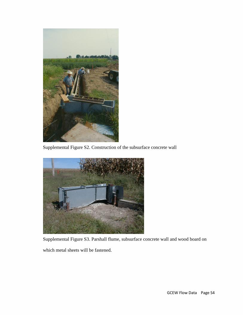
Supplemental Figure S2. Construction of the subsurface concrete wall
Supplemental Figure S3. Parshall flume, subsurface concrete wall and wood board on
which metal sheets will be fastened.

GCEW Flow Data Page S5
Supplemental Figure S4. Flume and wing wall made of sheet metal fastened to the top of
the subsurface concrete wall and interlocked concrete blocks.
Supplemental Figure S5. Flume and wing walls made of sections of sheet metal bolted to
the top of the concrete wall. The metal sheets can be removed to let field equipment drive
over the flume and sampling equipment.
S3. Derivation of SI units Parshall flume coefficients from USDI-BR ratings Because of the lack of geometric similarity between Parshall flumes of different sizes,
each standard flume was calibrated individually and has its own rating table. However, equations have been proposed for flumes of specific sizes that result in less than 1% error. The USDI Bureau of Reclamation [2001] gives the following general equation for standard Parshall flumes:
𝑄 = 𝐶 𝐻𝑛

GCEW Flow Data Page S6
Where:
Q is the flow rate in cubic feet per second
H is the measured head in feet,
C and n are coefficients determined for each size flume.
For flumes sizes 6”, and 9”, C and n are 2.06 and 1.58; and 3.07 and 1.53, respectively.
A similar equation can be written in the metric system of units:
𝑄𝑚 = 𝐶𝑚𝐻𝑚𝑛𝑚
Where:
Qm is the flow rate in cubic meters per second
Hm is the measured head in meter,
Cm and nm are coefficients determined for each size flume.
The relationship for C and n between the metric and English systems of units are:
𝐶𝑚 = 𝐶 ∗ 3.2808𝑛/3.28083
𝑛𝑚 = 𝑛
S4. Characteristics of the stream weirs that support stream gaging in GCEW.
Clear images are available on Google Earth using the coordinates given in Table 1. For weirs 9 and 11, the weirs are a few meters upstream of a road bridge while the footbridges are 20 to 30 m downstream of it. At weir 1, the weir and the foot bridge are both downstream of the road bridge.
Supplemental Figure S6. Weir 9 channel and bridge cross-section.

GCEW Flow Data Page S7
Supplemental Figure S7. Weir 11 channel and bridge cross-section
S5. Young’s Creek measurements Supplemental Table S3. Young’s Creek flow measurements and differences with values
estimated from the rating curve.
Date stage (ft)
Flowrate (cfs)
Rating flow (cfs)
Difference
1/31/2006 4.433 9 12.62 -26% 3/15/2006 4.583 18 23.65 -25%
5/4/2006 5.349 128 120.59 6% 6/1/2006 9.757 2037 1712.83 19%
3/18/2008 11.029 2501 2394.65 4% 4/30/2009 13.69 4905 4465.20 10%
S6. Flow metadata Daily flow volumes are available for all the GCEW sites, i.e. plots, fields, and stream
weirs site, from the Sustaining the Earth’s Watersheds, Agricultural Research Data System (STEWARDS) (www.ars.usda.gov/watersheds/stewards, accessed June 1, 2012) [Steiner et al. 2008, 2009a, 2009b; Sadler et al. 2008]. All data available through STEWARDS are in the public domain, and are not restricted by copyright. Sub-daily stage and flow data are also

GCEW Flow Data Page S8
available on request at the 5- or 15-min time step. Metadata document methods for obtaining these data and successive updates.
Eight of the flow gauges in the Mark Twain Lake watershed are owned and operated by USGS. Daily data for these sites can be found on the USGS National Water Information System (http://waterdata.usgs.gov/nwis, accessed June 1, 2012). Sub-daily data were obtained from USGS and are available on request. The Young’s Creek flow gauging station in the Mark Twain Lake Watershed is owned and operated by ARS. Daily flow volumes are available from STEWARDS and sub-daily data are available on request.
The flow data are maintained in three different structures. The first is when it is flow data downloaded from the ISCO sampler are uploaded to a desktop computer for review using the Flowlink 4® program. After weekly review, stage and time data are exported to ASCII files and uploaded to a highly relational Oracle® database for use by research scientists of the Cropping System and Water Quality (CSWQ) research unit. This database pre-existed the STEWARDS project, and the decision has been made to maintain the local database structure and content until the next platform migration project. Thus, steps needed to transform the local tables from the CSWQ format to the STEWARDS format were developed. The upload to STEWARDS is done annually, with STEWARDS maintained within 2 years of current data. The agency has committed to maintaining STEWARDS as the permanent public access to this data store. The data are available to the public at (http://www.nrrig.mwa.ars.usda.gov/stewards/stewards.html). See the navigation aid for SETWARDS below. Navigation aid for STEWARDS access to Goodwater Creek Experimental Watershed data.
• Click http://www.nrrig.mwa.ars.usda.gov/stewards/stewards.html • Click ‘OK’ • Click ‘tt’ icons in Missouri for short description of Goodwater Creek or Mark Twain Lake/Salt
River Basin. From that short description, click the hyperlink for the longer watershed description file.
o Click ‘X’ to exit the description • Hover over ‘Tools’ to display options in that section.
o ‘Summary by location’ displays data holdings across watersheds o ‘Select Research Location’ does the same as the direct method shown next.
• Click the blue pin labeled ‘Select Research Location, then click the drop-down arrow to display locations.
o Select Goodwater Creek or Mark Twain Lake/Salt River Basin. The display will zoom in on the selected watershed.
o The ‘tt’ map tips can be clicked for display of the unique SiteID or clickable descriptions of the individual measurement site.
o Under the Select Research Location box: The watershed description file can be accessed (same file as above). The data holdings can be examined for the selected watershed
Note: Viewing data in table or graph form is possible, but downloading is enabled only after signing in (new users need e-mail, name, and organization; existing users need only email). Assuming one wants data, click User Login from main screen. Once logged in, one can get data two ways. One is direct data access from the login box, which is ftp access to the whole STEWARDS data base (identified by the state/location codes, MOGC is Goodwater Creek and MOSR is Salt River). The other is by theme/parameter/site queries.

GCEW Flow Data Page S9
• Hover over ‘Tools’ button o Select ‘View Location Data’
One can search by theme or parameter, then select site of interest. Once selections are made, Click ‘Get data’
• There are three selections at the upper left of the new window. o Show graph gives a quick visualization in a time series plot. o Show metadata give the FGDC-compliant metadata for the GIS layer, in which entity
attributes contain some metadata about the measurements at that site. o Show methods lists the fields in the measurement descriptions
• There are also three additional download options o Location GIS files provides the GIS files relevant to the selected parameter o Site description provides the site description file o Location description provides the watershed description file.
• Assuming all three additional download options are clicked, Save to Text File (csv) delivers a download package to your PC, using the standard Windows file dialog box. This is a compressed (zipped) folder, containing:
o The data file itself, named by date and time, in csv form, e.g., ARS-DATA_mmddyyyyhhmmss(am/pm)
o A readme file with _README appended to the same name, in csv form o The methods description, e.g., ARS_Methods in pdf form o The site description, e.g., ARS_Sites in pdf form o The watershed description file, e.g., Goodwater Creek MO in html form o A compressed set of GIS files, e.g., MOGC_StewardsGIS.gdb o The GIS layer metadata, e.g., MOGC_WeirsAndFlumes_metadata in html form o The STEWARDS data use policy in pdf form
The data themes and methods tables in STEWARDS that are relevant to the flow data are shown below.

GCEW Flow Data Page S10
arcGIS feature class Table name ParameterDescription TopicID
MOGC_FieldWeirs MOGC_FieldWeirs_FlowBreakpoint Site identifier SiteID
Date & time DateTime
Stream stage, water, meters STAGE_HEIGHT_M
Discharge, rate, water, cubic meters per second FLOW_RATE_CMS
Discharge, volume, water, cubic meters VOL_CU_M
MOGC_FieldWeirs_FlowDaily Site identifier SiteID
Date & time DateTime
Discharge, volume, water, daily, cubic meters VOLUME_CU_M
MOGC_PlotFlumes MOGC_PlotFlumes_FlowBreakpoint Site identifier SiteID
Date & time DateTime
Discharge, rate, water, cubic meters per second FLOW_RATE_CMS
Discharge, volume, water, cubic meters VOL_CU_M
MOGC_PlotFlumes_FlowDaily Site identifier SiteID
Date & time DateTime
Discharge, volume, water, daily, cubic meters VOLUME_CU_M
MOGC_StreamWeirs MOGC_StreamWeirs_FlowBreakpoint Site identifier SiteID
Date & time DateTime
Stream stage, water, meters STAGE_HEIGHT_M
Discharge, rate, water, 2012 rating curve, cubic meters per second FLOW_RATE_CMS_2012
Discharge, volume, water, 2012 rating curve, cubic meters VOL_CU_M_2012
Discharge, rate, water, 1993 rating curve, cubic meters per second FLOW_RATE_CMS_1993
Discharge, volume, water, 1993 rating curve, cubic meters VOL_CU_M_1993
MOGC_StreamWeirs_FlowWithRainDaily Site Identifier SiteID
Date & time DateTime
Discharge, volume, water, 2012 rating curve, cubic meters VOLUME_CU_M_2012
Discharge, volume, water, 1993 rating curve, cubic meters VOLUME_CU_M_1993
Precipitation, no media, millimeters DEPTH_MM

GCEW Flow Data Page S11
arcGIS feature class Table name ParameterDescription TopicID
MOSR_StreamSamplers MOSR_StreamSamplers_FlowBreakpoint Site identifier SiteID
Date & time DateTime
Stream stage, water, meters STAGE_HEIGHT_M
Discharge, rate, water, cubic meters per second FLOW_RATE_CMS
Discharge, volume, water, cubic meters VOL_CU_M
MOSR_StreamSamplers_FlowDaily Date & time DateTime
Site identifier SiteID
Discharge, volume, water, daily, cubic meters VOLUME_CU_M

GCEW Flow Data Page S12
S7. Plots and fields management CS1 plots and Field 1 (F1) were managed in a mulch-till corn soybean cropping system,
with chisel plow or cultivation in the early spring, pre-planting application of fertilizers and herbicides, and incorporation of these inputs by cultivation followed by planting. One exception to this rotation was in 1995 when a very wet spring prevented any field operations until late June. In the field, sorghum was planted instead of corn because of its shorter growing season and a late December tillage was needed to remedy the compaction that resulted from field operations on wetter than normal soils.
CS2 plots were managed in a no-till corn soybean cropping system, with application of herbicides and fertilizers on planting day. Field 2 (F2) was similar to F1 from 1993 to 1996 but with sorghum instead of corn. Fertilizer rates were slightly lower in expectation of lower yields and nutrient uptake from sorghum than from corn. In 1997, the management was switched to a corn-soybean no-till system similar to the CS2 plots and in phase with that of F1. Fertilizer rates were lower than those of F1 because of expected lower rates with a no-till system than when fertilizers are incorporated.
From 1993 to 1996, CS5 plots were managed as a mulch-till corn-soybean-wheat system, with wheat a cover crop during all winters. In 1996, tillage stopped on these plots but the rotation was conserved.
From 1993 to 1996, Field 3 (F3) was managed as a corn-soybean-wheat no-till system, with wheat over the winter 1993, corn in 1994, and soybean in 1995 followed by a winter wheat crop harvested in June 1996. This management stopped in 1996; starting in 1997 and until 2001, F3 was managed as a corn-soybean no-till system, in phase with the systems on F1 and F2, with variable application rates of fertilizer and herbicides. Rates of nitrogen were calculated as a function of expected yields, themselves a function of the soil depth above the claypan. Rates of phosphorus and potassium were derived from soil P and K contents in1996 samples, assuming a 4 year-buildup. Fertilizers were only applied during the corn phase of the rotation.
S8. References. Sadler, E. J., J. L. Steiner, J. S. Chen, G. Wilson, J. Ross, T. Oster, D. James, B. Vandenberg, K.
Cole, and J. Hatfield. 2008. Sustaining the Earth's Watersheds-Agricultural Research Data System: data development, user interaction, and operations management, J. Soil and Water Conserv., 63(6):577-589, doi: 10.2489/jswc.63.6.577.
Steiner, J. L., E. J. Sadler., J. S. Chen, G. Wilson, D. James, B. Vandenberg, J. Ross, T. L. Oster, and K. Cole. 2008. Sustaining the Earth’s Watersheds – Agricultural Research Data System: overview of development and challenges. J. Soil and Water Conserv. 63(6):569-576, doi:10.2489/jswc.63.6.569.
Steiner, J. L., E. J. Sadler, J. L. Hatfield, G. Wilson, D. E. James, B. C. Vandenberg, J. D. Ross, T. L. Oster, and K. J. Cole. 2009a. Data management to enhance long-term watershed research: context and STEWARDS case study, J. Ecohydrology, 2:391-398, doi:10.1002/eco.89
Steiner, J. L., E. J. Sadler, G. Wilson, J. L. Hatfield, D. James, B. Vandenberg, J. S. Chen, T. Oster, J. D. Ross, and K. Cole. 2009b. STEWARDS watershed data system: system design and implementation, Trans. ASABE, 52(5):1523-1533.


