

Support vector machines (SVMs) Lecture 3
David Sontag New York University
Slides adapted from Luke Zettlemoyer, Vibhav Gogate, and Carlos Guestrin

Geometry of linear separators (see blackboard)
A plane can be specified as the set of all points given by:
Barber, Section A.1.1-4
Vector from origin to a point in the plane Two non-parallel directions in the plane
Alternatively, it can be specified as:
Normal vector (we will call this w)
Only need to specify this dot product, a scalar (we will call this the offset, b)

Linear Separators
! If training data is linearly separable, perceptron is guaranteed to find some linear separator
! Which of these is optimal?
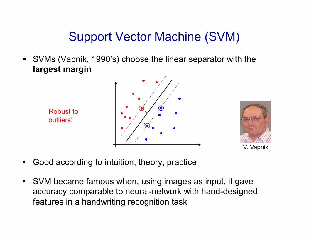
! SVMs (Vapnik, 1990’s) choose the linear separator with the largest margin
• Good according to intuition, theory, practice
• SVM became famous when, using images as input, it gave accuracy comparable to neural-network with hand-designed features in a handwriting recognition task
Support Vector Machine (SVM)
V. Vapnik
Robust to outliers!
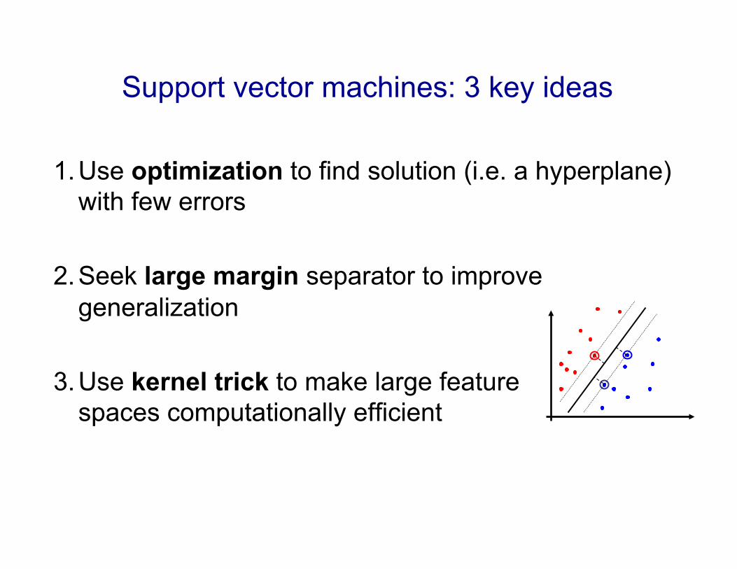
1. Use optimization to find solution (i.e. a hyperplane) with few errors
2. Seek large margin separator to improve generalization
3. Use kernel trick to make large feature spaces computationally efficient
Support vector machines: 3 key ideas
w.x
+ b
= +
1
w.x
+ b
= -1
w.x
+ b
= 0
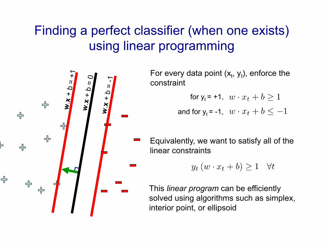
Finding a perfect classifier (when one exists) using linear programming
for yt = +1,
and for yt = -1,
For every data point (xt, yt), enforce the constraint
Equivalently, we want to satisfy all of the linear constraints
This linear program can be efficiently solved using algorithms such as simplex, interior point, or ellipsoid

Finding a perfect classifier (when one exists) using linear programming
Example of 2-dimensional linear programming (feasibility) problem:
For SVMs, each data point gives one inequality:
What happens if the data set is not linearly separable?
Weight space
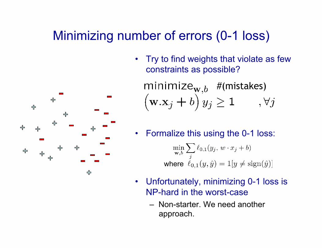
• Try to find weights that violate as few constraints as possible?
• Formalize this using the 0-1 loss:
• Unfortunately, minimizing 0-1 loss is NP-hard in the worst-case – Non-starter. We need another
approach.
#(mistakes)
Minimizing number of errors (0-1 loss)
where

Key idea #1: Allow for slack
For each data point: • If functional margin ≥ 1, don’t care • If functional margin < 1, pay linear penalty
w.x
+ b
= +
1
w.x
+ b
= -1
w.x
+ b
= 0
ξ2
ξ1
ξ3
ξ4
Σj ξj
- ξj ξj≥0
“slack variables”
We now have a linear program again, and can efficiently find its optimum
, ξ

Key idea #1: Allow for slack
w.x
+ b
= +
1
w.x
+ b
= -1
w.x
+ b
= 0
Σj ξj
- ξj ξj≥0
“slack variables”
, ξ
What is the optimal value ξj* as a function
of w* and b*?
If then ξj = 0
If then ξj =
Sometimes written as
ξ2
ξ1
ξ3
ξ4

Equivalent hinge loss formulation
Σj ξj - ξj ξj≥0
Substituting into the objective, we get:
, ξ
This is empirical risk minimization, using the hinge loss
The hinge loss is defined as
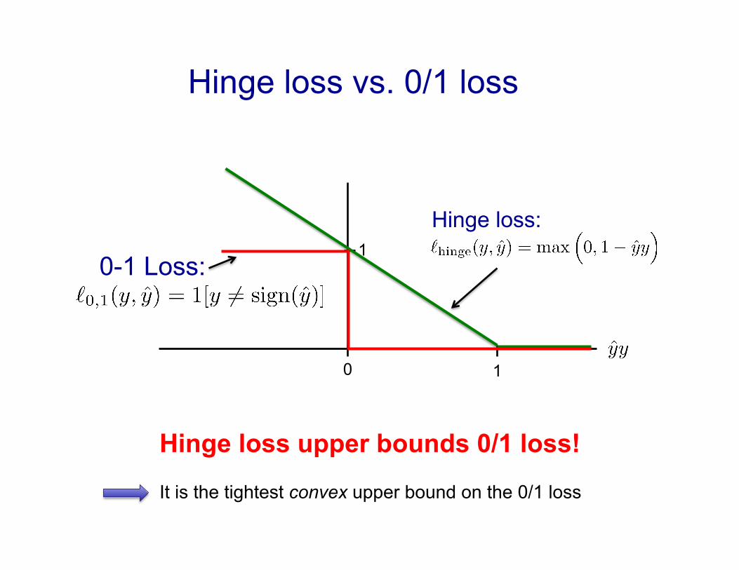
Hinge loss vs. 0/1 loss
1 0
1
Hinge loss upper bounds 0/1 loss!
It is the tightest convex upper bound on the 0/1 loss
Hinge loss:
0-1 Loss:
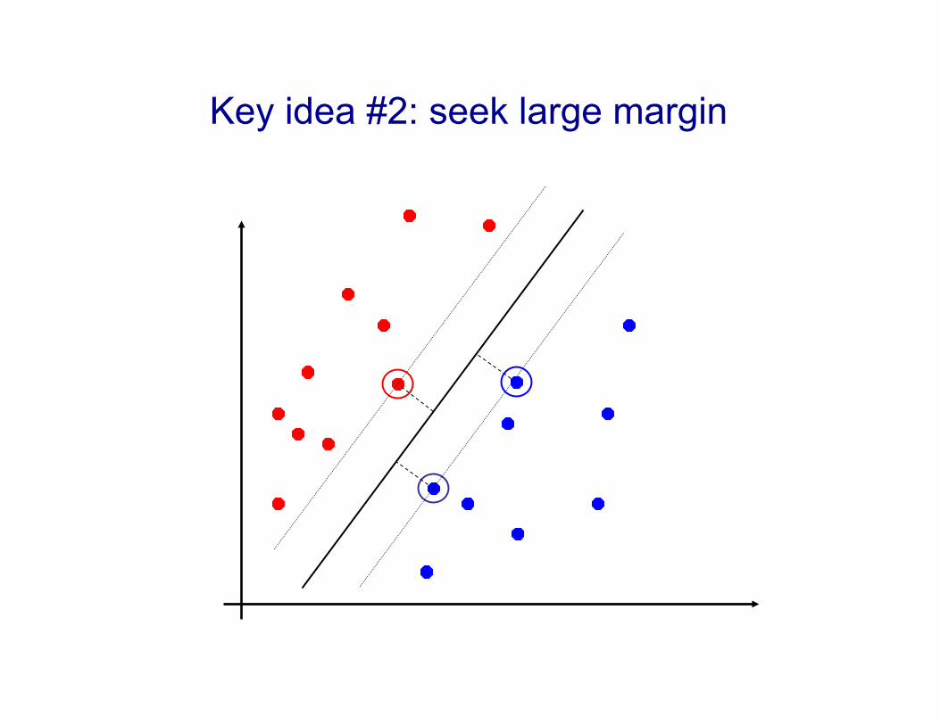
Key idea #2: seek large margin


