

Survival Analysis - A Self-Learning Text
RK
September 7, 2015
Abstract
This document contains a brief summary of the book “Survival Analysis - A Self-Learning Text”
1

Survival Analysis - A Self-Learning Text
Contents
1 Introduction to Survival Analysis 3
2 Kaplan-Meier Survival Curves and the Log-Rank Test 10
3 The Cox Proportional Hazards Model and its characteristics 16
4 Evaluating the Proportional Hazards Assumption 20
5 The Stratified Cox Procedure 26
6 Extension of the Cox Proportional Hazards Model for Time-Dependent Variables 34
7 Parametric Survival Models 40
8 Recurrent Event Survival Analysis 51
9 Competing Risks Survival Analysis 55
10 Takeaway 56
2

Survival Analysis - A Self-Learning Text
Context
I stumbled on to this book and was immediately drawn towards it because of its appealing format. Each
chapter contains the contents in a lecture book format, i.e. the left hand side of the page appears like a mini
power point deck and the right hand side elaborates the points on the left hand side. The structure of the
content for every chapter is same, i.e. Introduction, Abbreviated Outline, Objectives, Presentation, Detailed
Outline, Practice Exercises, Test, Answers to Practice Exercises. There are 10 chapters in the book that take
up 520 odd pages. There are additional 180 odd pages in the book that talk about various software packages
that can be used to do survival analysis. In this document, I will try to briefly summarize the book.
1. Introduction to Survival Analysis
Survival analysis is a collection of statistical procedures for data analysis for which the outcome variable of
interest is time until an event occurs. The time variable is usually referred to as survival time, because it gives
the time that an individual has “survived” over some follow-up period. The basic data structure is a tuple, i.e
(start, stop, event) where the the first two elements signifies the start and end time of the study, while
the third element signifies whether the event has occurred or not. The event might not occur for three reasons
� a person does not experience the event before the study ends
� a person is lost to follow-up during the study period
� a person withdraws from the study because of death of some other reason(competing risk)
There can be two types of censoring, left censoring and right censoring. Most of the survival analysis data
is right censored. Left censoring of data can occur when a person’s true survival time is less than or equal
to that person’s observed survival time. For example, we can track a person until they become HIV positive.
But the time to event will be left censored as we do not know the actual time of the first exposure.
The two key quantitative terms used in survival analysis are survivor function function and hazard func-
tion.The survivor function is fundamental to survival analysis, because survival probabilities for different
values of t provides a crucial summary information of the survival dataset. In theory, survivor functions are
smooth functions but empirical survivor functions are step functions. The hazard functions gives the instan-
taneous potential per unit time for the event to occur, given that the individual has survived up to time t.
A good analogy is a speedometer. Any speed that is registered on the speedometer tells the potential at the
moment you have looked at your speedometer, for how many miles you will travel in the next hour. The
hazard function is the same. It gives the probability of event occurring in the next instant given that the
subject has survived until that instant. The hazard function is also called conditional failure rate. The two
defining features of hazard function is that it is always non negative and it has no upper bound. The hazard
function of exponential distribution is constant. For a Weibull it is monotonically increasing or monotonically
decreasing. For a log normal distribution it is an inverted U shape. There is no known parametric distribution
that can give a U shaped hazard function.
The hazard model is of interest primarily because
� It is a measure of instantaneous potential whereas survival curve is a cumulative measure over time
� It may be used to identify a specific parametric form
� It is the vehicle by which math modeling of survival data is carried out
3

Survival Analysis - A Self-Learning Text
The equation connecting survivor and hazard function is :
S(t) = exp
(−∫ t
0
h(u)du
)
The three basic goals of survival analysis are
1. To estimate and interpret survivor and/or hazard functions from survival data.
2. To compare survivor and/or hazard functions.
3. To assess the relationship of explanatory variables to survival time.
The authors illustrate the basic layout for a computer analysis via leukemia remission dataset
data_leukemia <- read.table("data/gehan.dat")
data_leukemia[,3] <- as.numeric(data_leukemia[,3])
head(data_leukemia)
## group weeks relapse
## 1. treated 6 1
## 2. treated 6 1
## 3. treated 6 1
## 4. treated 6 0
## 5. treated 7 1
## 6. treated 9 0
table(data_leukemia$group,data_leukemia$relapse)
##
## 0 1
## control 0 21
## treated 12 9
An alternative format is the counting process format that is illustrated via another dataset
data_bladder <- read.table("data/bladder.dat", header = TRUE, stringsAsFactors = FALSE)
head(data_bladder)
## ID EVENT INTERVAL INTTIME START STOP TX NUM SIZE
## 1 1 0 1 0 0 0 0 1 1
## 2 2 0 1 1 0 1 0 1 3
## 3 3 0 1 4 0 4 0 2 1
## 4 4 0 1 7 0 7 0 1 1
## 5 5 0 1 10 0 10 0 5 1
## 6 6 1 1 6 0 6 0 4 1
In this kind of dataset, there can be multiple observations for each ID. There are recurrent events for individuals
and these are captured in this format
4

Survival Analysis - A Self-Learning Text
subset(data_bladder, ID==14)
## ID EVENT INTERVAL INTTIME START STOP TX NUM SIZE
## 22 14 1 1 3 0 3 0 3 1
## 23 14 1 2 6 3 9 0 3 1
## 24 14 1 3 12 9 21 0 3 1
## 25 14 0 4 2 21 23 0 3 1
The basic layout for understanding analysis is one that has four columns
1. Distinct ordered failure times t(f)
2. # of failures m(f)
3. # censored in [tf , t(f+1)] - The number censored between the current time and the next ordered failure
time
4. Risk set at t(f) - The collection of individuals survived at least till t(f)
For the remission data, one can get an empirical survival rate for the treated group as follows:
data_grp1 <- subset(data_leukemia, group=="treated")
fit <- with(data_grp1, survfit(Surv(weeks,relapse)~1, conf.type="none"))
summary(fit)
## Call: survfit(formula = Surv(weeks, relapse) ~ 1, conf.type = "none")
##
## time n.risk n.event survival std.err
## 6 21 3 0.857 0.0764
## 7 17 1 0.807 0.0869
## 10 15 1 0.753 0.0963
## 13 12 1 0.690 0.1068
## 16 11 1 0.627 0.1141
## 22 7 1 0.538 0.1282
## 23 6 1 0.448 0.1346
What is the use of the table of ordered failure times ?
The importance of the table of ordered failure times is that we can work with censored observations in analyzing
survival data. Even though censored observations are incomplete, in that we don’t know a person’s survival
time exactly, we can still make use of the information we have on a censored person up to the time we lose
track of him or her. Rather than simply throwing away the information on a censored person, we use all the
information we have on such a person up until time of censorship.
Crude statistics on the survival data set are ordinary average and hazard rate average. However these do not
take time in to consideration. To get a time element, one typically uses a non parametric estimator such as
Kaplan-Meier method.
5

Survival Analysis - A Self-Learning Text
fit <- with(data_leukemia, survfit( Surv(weeks, relapse) ~ group ))
plot(fit, lty = c(2, 1))
legend("topright", legend = c("treated", "control"),
lty =c(1, 2),bty = "n")
abline(h = 0.5, col = "sienna", lty = 3)
0 5 10 15 20 25 30 35
0.0
0.2
0.4
0.6
0.8
1.0
treatedcontrol
One should also take in to consideration confounding effects. It is possible that some covariate is clouding the
analysis. The following shows average logWBC for treatment and control subjects. The density plot shows
that there are differences.
data_er <- read.csv("data/extended_remission_data.csv")
data_er_1 <- subset(data_er, grp==1)
data_er_2 <- subset(data_er, grp==2)
plot(density(data_er_1$logWBC), xlim = c(0, 8), lty = 2, ylim = c(0, .6),
xlab = "", main = "")
par(new=TRUE)
plot(density(data_er_2$logWBC), xlim = c(0, 8), lty = 1, ylim = c(0, .6),
xlab = "",main = "")
legend("topright", legend = c("treated", "control"), lty = c(2, 1), bty = "n")
6

Survival Analysis - A Self-Learning Text
0 2 4 6 8
0.0
0.1
0.2
0.3
0.4
0.5
0.6
Den
sity
0 2 4 6 8
0.0
0.1
0.2
0.3
0.4
0.5
0.6
Den
sity
treatedcontrol
One might have to take this variable in the covariates to adjust for confounding. By stratification and analyzing
the survival probabilities, we get the following plots:
data_er <- read.csv("data/extended_remission_data.csv")
data_er_1 <- data_er[data_er$logWBC <=2.5, ]
data_er_2 <- data_er[data_er$logWBC >2.5, ]
fit_er_1 <- with(data_er_1, survfit( Surv(time, event) ~ grp ))
fit_er_2 <- with(data_er_2, survfit( Surv(time, event) ~ grp ))
par(mfrow=c(1,2))
plot(fit_er_1, lty = c(1, 2), main = "low log WBC")
legend("topright", legend = c("treated", "control"), lty =c(1, 2), bty = "n")
abline(h = 0.5, col = "sienna", lty = 3)
plot(fit_er_2, lty = c(1, 2), main = "high log WBC")
legend("topright", legend = c("treated", "control"), lty =c(1, 2),bty = "n")
abline(h = 0.5, col = "sienna", lty = 3)
7

Survival Analysis - A Self-Learning Text
0 5 10 15 20 25 30 35
0.0
0.2
0.4
0.6
0.8
1.0
low log WBC
treatedcontrol
0 5 10 15 20 25 300.
00.
20.
40.
60.
81.
0
high log WBC
treatedcontrol
The math behind the survival analysis, regression and logistic regression look very similar. In the survival
analysis, the outcome variable is time to event (with censoring). In a linear regression the effect is measured
via β, the regression coefficient. In a logistic regression, the effect is measured via eβ and in survival analysis,
the effect is again measured via eβ which is called hazard ratio. One thing that is different in survival analysis
is that the covariates are coded in such a way that hazard ratio of the control to treatment is greater than 1.
In this way, one can easily understand that hazard of a control group is x times the hazard of a treated group.
The last part of the chapter covers the difference between independent, random and non-information censoring.
The best way to understand these three terms are by an analogy
Imagine that there are two math teachers and you want to recruit one for your school. You recruit
both on a contract basis and ask them to take classes for a month. The classes run in a peculiar
way. Each student can decide to take a test at the end of each week. If he passes the test, he is
taken out of the class, else he continues. There are dropouts too from each of the classes. The
surviving population in both the classes can be used to gauge the effectiveness of the math teachers.
In an independent censoring scenario, the profile of student number of students who drop out of
a class is representative of the students who are still in the class. In an random censoring, the %
of students who drop out of each class is same. This means that there is equal probability that
someone drops out of either class. Note that random censoring is more strict that independent
censoring. The latter merely needs random dropouts at a covariate level whereas former requires
random dropouts across various covariate levels. Lastly non-information censoring means that the
survival time distribution gives information about the censored time distribution.Imagine a case
where whenever a student fails, the student’s close friend also drops out. This is a case where the
survival distribution totally determines the censored distribution.
An important point to note about Random censoring and Independent censoring is:
8

Survival Analysis - A Self-Learning Text
� Random censoring within Group A and within Group B ⇒ Independent censoring
� Independent censoring within Group A and within Group B 6⇒ Random censoring
Many of the analytic techniques discussed in the chapters such as Kaplan-Meier survival estimation, the log
rank test, and the Cox model, rely on an assumption of independent censoring for valid inference in the
presence of right-censored data.
9

Survival Analysis - A Self-Learning Text
2. Kaplan-Meier Survival Curves and the Log-Rank Test
Given a dataset with (start,end,event), one would like to get an estimate of the survival probabilities.
Kaplan-Meier is a non parametric method to estimate the survival probabilities at a given time instant. To
estimate the survival probability at a given time, we make use of the risk set that includes the information we
have on a censored rather than simply throw away all the information on the censored person.
The data structure used to do KM estimation is ordered failure times. This is one aspect that is very different
from the usual statistical methods. The ordering of events is important in estimating parameters of the model
rather than the actual timing of the events.The data structure has four columns and they are
� ordered failure times
� # of failures
� # censored in the time interval
� Risk set
The chapter starts off with a simple example to illustrate the key idea of KM estimation. The following code
creates the relevant numbers
data_leukemia <- read.table("data/gehan.dat")
data_leukemia[,3] <- as.numeric(data_leukemia[, 3])
data_grp1 <- subset(data_leukemia, group == "control")
fit_1 <- with(data_grp1,
survfit(Surv(weeks,relapse) ~ 1,
conf.type = "none"))
print(summary(fit_1))
## Call: survfit(formula = Surv(weeks, relapse) ~ 1, conf.type = "none")
##
## time n.risk n.event survival std.err
## 1 21 2 0.9048 0.0641
## 2 19 2 0.8095 0.0857
## 3 17 1 0.7619 0.0929
## 4 16 2 0.6667 0.1029
## 5 14 2 0.5714 0.1080
## 8 12 4 0.3810 0.1060
## 11 8 2 0.2857 0.0986
## 12 6 2 0.1905 0.0857
## 15 4 1 0.1429 0.0764
## 17 3 1 0.0952 0.0641
## 22 2 1 0.0476 0.0465
## 23 1 1 0.0000 NaN
data_grp2 <- subset(data_leukemia, group == "treated")
fit_2 <- with(data_grp2,
survfit(Surv(weeks,relapse) ~ 1,
conf.type = "none"))
print(summary(fit_2))
10

Survival Analysis - A Self-Learning Text
## Call: survfit(formula = Surv(weeks, relapse) ~ 1, conf.type = "none")
##
## time n.risk n.event survival std.err
## 6 21 3 0.857 0.0764
## 7 17 1 0.807 0.0869
## 10 15 1 0.753 0.0963
## 13 12 1 0.690 0.1068
## 16 11 1 0.627 0.1141
## 22 7 1 0.538 0.1282
## 23 6 1 0.448 0.1346
The survival probabilities for the treatment and control group are evaluated based on simple binomial model
where the sample size is the number of people in the risk set and the number of successes are represented by
the number of events. The most important thing to note is that the risk set contains people who have not
been censored during the time interval considered. Thus KM estimation does not throw away the information.
Any KM formula for a survival probability is limit of product terms up to the survival week being specified.
That is why the KM formula is often referred to as product-limit formula. The KM plots for two groups can
be easily obtained via Surv function.
fit <- with(data_leukemia, survfit( Surv(weeks, relapse) ~ group ))
plot(fit, lty = c(2, 1))
legend("topright", legend = c("treated", "control"),
lty =c(1, 2),bty = "n")
abline(h = 0.5, col = "sienna", lty = 3)
0 5 10 15 20 25 30 35
0.0
0.2
0.4
0.6
0.8
1.0
treatedcontrol
11

Survival Analysis - A Self-Learning Text
The general formula for Kaplan-Meier estimation is
S(t(f)) = P r(T > t(f) = S(t(f−1)) ∗ P r(T > t(f)|T ≥ t(f))
The statistic used to compare two survival curves is called log rank test statistic. This is a large sample χ2
statistic in which categories are the set of ordered failure times. The idea behind this test is that at each
failure point, given the risk set of each group and total failures of each of group, an expected failure count is
computed for each group. This expected count is compared to the observed count
Log rank statistic =(O2 − E2)2
Var(O2 − E2)∼ χ2(1)
For the remission dataset, one can obtain the log-rank statistic as follows:
with(data_leukemia, survdiff(Surv(weeks, relapse) ~ group))
## Call:
## survdiff(formula = Surv(weeks, relapse) ~ group)
##
## N Observed Expected (O-E)^2/E (O-E)^2/V
## group=control 21 21 10.7 9.77 16.8
## group=treated 21 9 19.3 5.46 16.8
##
## Chisq= 16.8 on 1 degrees of freedom, p= 4.17e-05
As one see that pvalue is significant and hence the survivor function for the two groups is different.
Variations of the log-rank test can be done by using ρ argument in the function. For example the following
code weighs each term in the chi-square statistic based on the survival probabilities
with(data_leukemia, survdiff(Surv(weeks, relapse) ~ group, rho = 1))
## Call:
## survdiff(formula = Surv(weeks, relapse) ~ group, rho = 1)
##
## N Observed Expected (O-E)^2/E (O-E)^2/V
## group=control 21 14.55 7.68 6.16 14.5
## group=treated 21 5.12 12.00 3.94 14.5
##
## Chisq= 14.5 on 1 degrees of freedom, p= 0.000143
The survivor function testing across several groups also follows the same procedure. The chapter uses vets
dataset
data_vets <- read.table("data/vets.dat", header= FALSE)
temp <- t(sapply(data_vets[,1],
function(z){
temp <- unlist(strsplit(as.character(data_vets[1, 1]),
12

Survival Analysis - A Self-Learning Text
split = ""))
c(temp[1], paste0(temp[-1], collapse = ""))
}
)
)
data_vets$treatment <- as.numeric(temp[,1])
data_vets$celltype <- temp[,2]
data_vets <- data_vets[,c(-1)]
colnames(data_vets) <- c("time", "perf", "dis", "age",
"prior","status","treatment","celltype")
data_vets$perf_cat <- cut(data_vets$perf, c(0,59,74,199))
The KM curves for each of the categorized groups are
fit <- with(data_vets, survfit( Surv(time, status) ~ perf_cat))
plot(fit, lty = c(1, 2, 3), col = rainbow(3))
legend("topright", legend = c("0-59", "59-74", "75-100"),
lty =c(1, 2, 3),bty = "n", col = rainbow(3))
abline(h = 0.5, col = "sienna", lty = 3)
0 200 400 600 800 1000
0.0
0.2
0.4
0.6
0.8
1.0
0−5959−7475−100
with(data_vets, survdiff(Surv(time, status) ~ factor(perf_cat)))
## Call:
## survdiff(formula = Surv(time, status) ~ factor(perf_cat))
##
13

Survival Analysis - A Self-Learning Text
## N Observed Expected (O-E)^2/E (O-E)^2/V
## factor(perf_cat)=(0,59] 52 50 26.3 21.36 28.22
## factor(perf_cat)=(59,74] 50 47 55.2 1.21 2.19
## factor(perf_cat)=(74,199] 35 31 46.5 5.18 8.44
##
## Chisq= 29.2 on 2 degrees of freedom, p= 4.61e-07
The conclusion from the above log-rank test is that the survival curve across various performance categories
are different There are many alternatives to the log rank test in which the summed observed minus expected
are weighed differently. For Wilcoxon test, weights are chosen in such a way that more emphasis is placed on
the information at the beginning of the survival curve where the number at risk is large allowing early failures
to receive more weight than later failures.
Teststatistic :
(∑f w(t(f))(mif − eif )
)2Variance
(∑f w(t(f))(mif − eif )
)The alternatives to log-rank test depends on choosing different weighing mechanisms. The book gives the
following guidelines for choosing a test For the above vets.dat, we can use an alternative test with ρ as the
input argument
with(data_vets, survdiff(Surv(time, status) ~ factor(perf_cat),rho=1))
## Call:
## survdiff(formula = Surv(time, status) ~ factor(perf_cat), rho = 1)
##
## N Observed Expected (O-E)^2/E (O-E)^2/V
## factor(perf_cat)=(0,59] 52 35.8 16.3 23.27 44.2
## factor(perf_cat)=(59,74] 50 21.0 28.2 1.84 4.7
## factor(perf_cat)=(74,199] 35 10.6 22.9 6.62 15.4
##
## Chisq= 46.1 on 2 degrees of freedom, p= 9.93e-11
The results are not too different from the original χ2 text.
The chapter ends with the following suggestions about using various alternative tests
� Results of different weightings usually lead to similar conclusions
� The best choice is test with most power
� Power depends on how the null is violated
� There may be a clinical reason to choose a particular weighting
� Choice of weighting should be apriori
The chapter ends with a discussion of Greenwood’s formula for computing the confidence intervals for
survival curves. In R, you get the confidence intervals whenever you use the survfit function.
For example, for the remission data, you can fit a confidence interval for the survival probability curve for the
control group as follows
14

Survival Analysis - A Self-Learning Text
data_leukemia <- read.table("data/gehan.dat")
data_leukemia[,3] <- as.numeric(data_leukemia[, 3])
data_grp1 <- subset(data_leukemia, group == "control")
fit_1 <- with(data_grp1, survfit(Surv(weeks,relapse) ~ 1))
plot(fit_1,conf.int=TRUE, col =c("green","red","red"))
abline(h = 0.5, col = "sienna", lty = 3)
0 5 10 15 20
0.0
0.2
0.4
0.6
0.8
1.0
This chapter sets the tone for the book by starting with the simplest estimator, the Kaplan-Meier estimator
which is a non parametric estimate. If you understand the math behind it, the whole procedure seems very
simple. However the power of such models is that there is no assumption whatsoever that goes in the modeling
and inference tasks.
15

Survival Analysis - A Self-Learning Text
3. The Cox Proportional Hazards Model and its characteristics
The chapter starts with leukemia remission data and shows the output from three models fitted to that data.
data_er <- read.csv("data/extended_remission_data.csv")
#Recoded group so that control has higher hazard ratio
data_er$grp <- factor( data_er$grp - 1 )
fit1 <- with(data_er, coxph(Surv(time, event) ~grp))
fit2 <- with(data_er, coxph(Surv(time, event) ~grp + logWBC))
fit3 <- with(data_er, coxph(Surv(time, event) ~grp*logWBC))
Model-1
coef exp(coef) se(coef) z pgrp1 1.57 4.82 0.41 3.81 0.00
Model-2
coef exp(coef) se(coef) z pgrp1 1.39 4.00 0.42 3.26 0.00
logWBC 1.69 5.42 0.34 5.03 0.00
Model-3
coef exp(coef) se(coef) z pgrp1 2.37 10.75 1.71 1.39 0.16
logWBC 1.87 6.50 0.45 4.15 0.00grp1:logWBC -0.32 0.73 0.53 -0.60 0.55
One can see that the model output has a similar structure to that of a regression output. In fact, the only
additional column is that of hazard ratio. The hazard ratio is equivalent to ecoef, that gives an estimate of
each variable adjusted for the other variables in the model. Model-3 output shows that the interaction effect
is not statistically significant. One can also do a simple anova test to infer the strength of the covariates.
drop1(fit3)
## Single term deletions
##
## Model:
## Surv(time, event) ~ grp * logWBC
## Df AIC
## <none> 145.30
## grp:logWBC 1 143.66
This shows that the interaction term can be dropped from Model-3. One can also compute difference in
−2 log likelihood between two nested models and compute the null on the covariate coefficients.
16

Survival Analysis - A Self-Learning Text
chistat <- -2*( (summary(fit2))$loglik[2] - (summary(fit3))$loglik[2])
1- pchisq(chistat, 1)
## [1] 0.5488232
A similar test can be performed between Model-1 and Model-2.
chistat <- -2*( (summary(fit1))$loglik[2] - (summary(fit2))$loglik[2])
1- pchisq(chistat, 1)
## [1] 3.587325e-08
In this case, the test is significant, which says that the log WBC is a variable worth considering.
The reason for showing the output of the three models is to drive home that the analysis of the model output
is similar to regression output analysis or logistic regression output analysis. The advantage of prop hazard
model is that you can draw adjusted survival curves, i.e survival curves adjusted for the covariates.
Cox PH model
h(t,X) = h0(t)e∑p
i=1 βiXi
where h0(t) is the baseline hazard that involves t but not the X’s. The exponential term in the plain vanilla
Cox model is time independent. If time dependent variables are considered, then it is called a extended Cox
Model. What are the characteristics of the model that makes it popular ?
� It is a semi-parametric model. A parametric model is one whose functional form is completely specified,
except for the values of the unknown parameters. Unlike such a model, Cox is a semi-parametric model,
i.e. baseline function is not specified
� It is robust, i.e. it will closely approximate the correct parametric model
� Even though baseline hazard is not specified, reasonably good estimates of regression coefficients, hazard
ratios of interest and adjusted survival curves can be obtained for a wide variety of data situations
� The form always ensures that the fitted model will always give estimated hazards that are non-negative.
� The measure of effect, called the hazard ratio, is calculated without having to estimate the baseline
intensity
� Survivor and Hazard curves can be estimated for the Cox model even though the baseline hazard function
is not specified
� Cox model is preferred over logistic model when survival time information is available and there is
censoring
Why is the procedure called Partial likelihood ?
The likelihood used is called Partial likelihood rather than (complete) likelihood function because the likelihood
considers probabilities only for those subjects who fail, and does not explicitly consider probabilities for those
subjects who are censored. Thus the likelihood for the Cox model does not consider probabilities for all
subjects, and so it is called a partial likelihood. Another point to note is that even though the partial likelihood
focuses on subjects who fail, survival time information prior to censorship is used for those subjects who are
censored.
One thing that is different from regression framework is the way one codes variables for treatment and placebo.
In a regression framework, one typically codes treatment as 1 and placebo as 0. In Cox model, the placebo is
17

Survival Analysis - A Self-Learning Text
coded as 1 and treatment as 0 so that it is easy to interpret hazards ratio greater than 1 than less than 1.
HR = exp
(p∑i=1
βi(X∗i −Xi)
)
The advantage of using Cox regression is that one can obtain adjusted survival curves. Here is the code to
compute the adjusted survival curves
fit2 <- with(data_er, coxph(Surv(time,event)~grp+logWBC))
temp_grp1 <- subset(data_er, grp==0)
temp_grp1$logWBC <- mean(data_er$logWBC)
temp_grp2 <- subset(data_er, grp==1)
temp_grp2$logWBC <- mean(data_er$logWBC)
plot(survfit(fit2,newdata=temp_grp1), col="blue")
par(new=T)
plot(survfit(fit2,newdata=temp_grp2),col = "red")
legend("topright", legend=c("treated","control"), lty=c(1,1), col = c("blue", "red"),bty="n")
0 5 10 15 20 25 30 35
0.0
0.2
0.4
0.6
0.8
1.0
0 5 10 15 20 25 30 35
0.0
0.2
0.4
0.6
0.8
1.0
treatedcontrol
The general formulae for adjusted survival curves comparing two groups are
Exposed Subjects S(t,X) =(S0(t)
)exp(β1(0)+∑
i6=1 βi(X∗i −Xi))
Unexposed Subjects S(t,X) =(S0(t)
)exp(β1(1)+∑
i6=1 βi(X∗i −Xi))
18

Survival Analysis - A Self-Learning Text
The Breslow’s estimator for the baseline cumulative hazard function is
H0(t) =∑ti≤t
h0(t) =∑ti≤t
1∑j∈Rj
eβxj
where h0(t) = 0 if t is not the event time.
What is the basic assumption in PH model ?
The basic assumption is that hazard ratio is not time dependent, i.e.
h(t,X∗)
h(t,X)= θ
This means that if the hazards cross for different strata, then PH assumption is questionable. What are the
options available if the PH assumption is not valid
� analyze by stratifying on the exposure variable; that is, do not fit any model, and, instead obtain
Kaplan-Meier curves for each exposure group separately
� start the analysis at delayed time stamp, and use a Cox PH model on three-day survivors
� fit Cox model for < t1 days and a different Cox model for > t1 to get two different hazard ratio estimates,
one for each of these two lime periods
� fit a modified Cox model that includes a time-dependent variable which measures the interaction of
exposure with time. This model is called an extended Cox model.
One of the biggest learnings from this chapter is the lottery example. It is a beautiful example that shows
that only the order of failure times matter and not the exact time at which the failures happen. The number
of lottery tickets with each individual acts as a covariate. This simple example makes it loud and clear that
The Cox likelihood is determined by the order of events and censorship and not by the distribution
of outcome variables.
The last section of the chapter is very interesting. It talks about the choice one has to make while deciding the
scale of the outcome variable. Should one choose time-on-study as the event time or time-on-calendar as the
event time ? The time-on-study makes sense if all the subjects are equally at risk at the beginning of the study.
This could happen in a clinical trial. However in an observational study, there is a high chance that whatever
time frame you are looking at, the time-on-study might give wrong survival probability estimates. Hence in
such cases calendar-time could be an appropriate choice. In a time-on-study , the risk set is closed cohort.
In calendar-time, the risk set is a open cohort. There is an alternate way to think about calendar-time. Why
not add it is a covariate in the time-on-study scale.
The guidelines given in the book for choosing between h(a,X) and h(t,X, a0), where a stands for the age
variable, are
� Prefer h(a,X) provided
– age is stronger determinant of outcome than time-on-study
– h0(a) is unspecified, so that age is not modeled as a covariate and hence avoids mis specifying the
model
� Prefer h(a,X, a0) provided
– time on study is stronger determinant than the age
– age at entry is effectively controlled in the model using a linear or quadratic term
19

Survival Analysis - A Self-Learning Text
4. Evaluating the Proportional Hazards Assumption
This chapter talks about three methods to evaluate the PH assumption.
Graphical Approach : Log-Log Plots
If we use a Cox PH model and we plot the estimated log-log survival curves for individuals on the same
graph,the two plots would be approximately parallel. The distance between the two curves is the linear
expression involving the differences in predictor values, which does not involve time. Note, in general, if the
vertical distance between two curves is constant, then the proportional hazards assumption holds good. The
parallelism of log-log survival plots for the Cox PH model provides us with a graphical approach for assessing
the PH assumption. That is, if a PH model is appropriate for a given set of predictors, one should expect that
empirical plots of log-log survival curves for different individuals will be approximately parallel.
By empirical plots, we mean plotting log-log survival curves based on Kaplan-Meier (KM) estimates that do
not assume an underlying Cox model. Alternatively, one could plot log-log survival curves which have been
adjusted for predictors already assumed to satisfy the PH assumption but have not included the predictor
being assessed in a PH model. Let us take the extended remission dataset and check PH assumption for each
covariate. KM plot for treatment and control shows that PH assumption is satisfied
data_er <- read.table("data/anderson.dat")
colnames(data_er) <- c("time", "event", "sex", "logWBC", "grp")
data_er$wb_cat <- cut(data_er$logWBC, c(0,2.3,3,8))
fit <- with(data_er, survfit(Surv(time,event)~grp))
plot(fit, fun="cloglog",main = "",log="x",col= c("blue","green"))
1 2 5 10 20
−2.
0−
1.5
−1.
0−
0.5
0.0
0.5
1.0
20

Survival Analysis - A Self-Learning Text
KM plot for logWBC categories shows that for data greater than 10 years, PH assumption is satisfied
fit <- with(data_er, survfit(Surv(time,event)~wb_cat))
plot(fit, fun="cloglog",main = "",log="x",col= c("blue","green","red"))
1 2 5 10 20
−2
−1
01
21

Survival Analysis - A Self-Learning Text
KM plot for sex shows that for PH assumption is not satisfied
fit <- with(data_er, survfit(Surv(time,event)~sex))
plot(fit, fun="cloglog",main = "",log="x",col= c("blue","green"))
1 2 5 10 20
−3.
0−
2.5
−2.
0−
1.5
−1.
0−
0.5
0.0
0.5
22
Survival Analysis - A Self-Learning Text
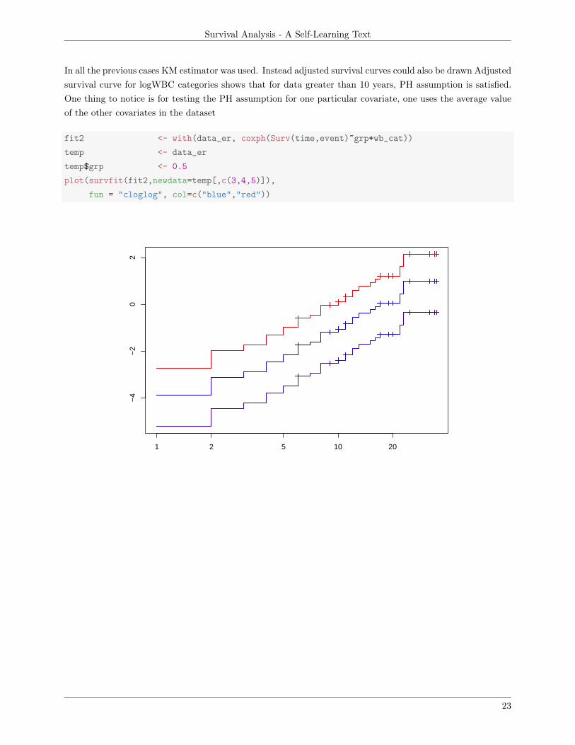
In all the previous cases KM estimator was used. Instead adjusted survival curves could also be drawn Adjusted
survival curve for logWBC categories shows that for data greater than 10 years, PH assumption is satisfied.
One thing to notice is for testing the PH assumption for one particular covariate, one uses the average value
of the other covariates in the dataset
fit2 <- with(data_er, coxph(Surv(time,event)~grp+wb_cat))
temp <- data_er
temp$grp <- 0.5
plot(survfit(fit2,newdata=temp[,c(3,4,5)]),
fun = "cloglog", col=c("blue","red"))
1 2 5 10 20
−4
−2
02
23

Survival Analysis - A Self-Learning Text
Adjusted survival curve for sex shows that for PH assumption is not satisfied
fit2 <- with(data_er, coxph(Surv(time,event) ~ grp + logWBC + sex))
temp <- data_er
temp$grp <- mean(temp$grp)
temp$logWBC <- mean(temp$logWBC)
plot(survfit(fit2, newdata = temp),
fun = "cloglog", col = c("blue", "red"))
1 2 5 10 20
−5
−4
−3
−2
−1
01
The Goodness of Fit Testing Approach
The test is based on Schoenfeld residuals. For each predictor in the model, Schoenfeld residuals are defined
for every subject who has an event. The way to compute the covariate residual for a subject is to subtract
the weighted average of the covariate from the observed value. The idea behind the statistical test is that if
the PH assumption holds for a particular covariate then the Schoenfeld residuals for that covariate will not be
related to survival time. The implementation of the test is a three-step process :
1. Run a Cox PH model and obtain Schoenfeld residuals for each predictor.
2. Create a variable that ranks the order of failures. The subject who has the first (earliest) event gets a
value of 1, the next gets a value of 2, and so on.
3. Test the correlation between the variables created in the first and second steps. The null hypothesis is
that the correlation between the Schoenfeld residuals and ranked failure time is zero.
The following results show that PH assumption holds good for grp and logWBC
24

Survival Analysis - A Self-Learning Text
fit2 <- with(data_er, coxph(Surv(time, event)~ grp + logWBC))
print(cox.zph(fit2))
## rho chisq p
## grp 0.00451 0.000542 0.981
## logWBC 0.02764 0.034455 0.853
## GLOBAL NA 0.034529 0.983
The following results show that PH assumption holds good for grp and logWBC but not for sex
fit2 <- with(data_er, coxph(Surv(time,event) ~ grp + logWBC + sex))
print(cox.zph(fit2))
## rho chisq p
## grp -0.1017 0.344 0.5578
## logWBC 0.0595 0.161 0.6883
## sex -0.3684 4.076 0.0435
## GLOBAL NA 4.232 0.2374
In the table above, one needs to row titled, GLOBAL. It is the result of a test of the global null hypothesis that
proportionality holds. The relatively small p-value tells us that we have a big problem with the proportionality
assumption.
Using Time-Dependent Covariates
This method involves using a time dependent function of the covariates in order to capture the effect. Typically
the choices of g(t) for the covariate δ(Xg(t)) are
g(t) = t
g(t) = log t
g(t) = Heaviside function
Using this as the covariate, one fits a proportional cox model and checks for statistical significance of the
coefficient δ .The number of δ’s that will appear in the model will depend on the covariates that are suspicious
of PH violation.
25

Survival Analysis - A Self-Learning Text
5. The Stratified Cox Procedure
The ”stratified Cox model” is a modification of the Cox proportional hazards (PH) model that allows for
control by ”stratification” of a predictor that does not satisfy the PH assumption. Predictors that are assumed
to satisfy the PH assumption are included in the model, whereas the predictor being stratified is not included.
data_er <- read.table("data/anderson.dat")
colnames(data_er) <- c("time", "event", "sex", "logWBC", "grp")
fit <- with(data_er,
coxph(Surv(time,event) ~ grp + logWBC + sex))
print(fit)
## Call:
## coxph(formula = Surv(time, event) ~ grp + logWBC + sex)
##
##
## coef exp(coef) se(coef) z p
## grp 1.504 4.498 0.462 3.26 0.0011
## logWBC 1.682 5.376 0.337 5.00 5.8e-07
## sex 0.315 1.370 0.455 0.69 0.4887
##
## Likelihood ratio test=47.2 on 3 df, p=3.17e-10
## n= 42, number of events= 30
One can see that the coefficient of sex is not significant. One can also do use cox.zph to check for PH
assumption violation.
print(cox.zph(fit))
## rho chisq p
## grp -0.1017 0.344 0.5578
## logWBC 0.0595 0.161 0.6883
## sex -0.3684 4.076 0.0435
## GLOBAL NA 4.232 0.2374
The results show that sex variable does not satisfy PH. The variable that do not satisfy PH assumption are
used in stratified COX procedure. The code to perform stratified cox is a slight modification of prop hazard
model. In the following code, the covariate is entered as strata(sex).
data_er <- read.table("data/anderson.dat")
colnames(data_er) <- c("time", "event", "sex", "logWBC", "grp")
data_er$wb_cat <- cut(data_er$logWBC, c(0,2.3,3,8))
fit <- with(data_er, coxph(Surv(time,event)~grp +
logWBC + strata(sex)))
26

Survival Analysis - A Self-Learning Text
print(((fit)))
## Call:
## coxph(formula = Surv(time, event) ~ grp + logWBC + strata(sex))
##
##
## coef exp(coef) se(coef) z p
## grp 0.998 2.713 0.474 2.11 0.035
## logWBC 1.454 4.279 0.344 4.22 2.4e-05
##
## Likelihood ratio test=32.1 on 2 df, p=1.09e-07
## n= 42, number of events= 30
The computer results show that the log WBC and grp variables are included in the model listing, whereas the
sex variable is not included; rather, the model stratifies on the sex variable, as indicated at the bottom of
the output. Note that the sex variable is being adjusted by stratification, whereas log WBCis being adjusted
by its inclusion in the model along with grp. Another important aspect to note is that sex variable is not
included in the model summary because it is controlled by stratification.
The basic idea behind Stratified Cox is that different baseline hazard functions are fit for various strata. The
covariates do not contain the variable that is being stratified.
The general Stratified Cox Model is
hg(t,X) = h0g exp(β1X1 + β2X2 + . . .+ βpXp), g = 1, 2, . . . k∗, strata
The stratified partial likelihood function is
L = L1 × L2 × . . . Lk∗
The above form means that you compute likelihood for each strata and multiply the likelihoods.
There are two types of stratified cox models that can be built. One where there is no interaction, i.e β’s
in the model are the same for each subscript g. The no-interaction assumptions means that the variables
being stratified are assumed not to interact with X’s in the model. In a model that allows interaction, you fit
separate models for each strata. One way to get an understanding an interaction is to plot the curves for each
combination of grp and sex
27

Survival Analysis - A Self-Learning Text
0 5 10 15 20 25 30 35
0.0
0.2
0.4
0.6
0.8
1.0
treatment−femaleplacebo−femaletreatment−maleplacebo−male
Another way to check whether there is interaction or not, is by fitting separate models to each of the strata
and seeing whether the time invariant covariates have similar values
temp0 <- subset(data_er, sex == 0) # male
temp1 <- subset(data_er, sex == 1) # female
fit <- with(data_er,
coxph(Surv(time,event)~ grp + logWBC + strata(sex)))
fit0 <- with(temp0, coxph(Surv(time, event) ~ grp + logWBC ) )
fit1 <- with(temp1, coxph(Surv(time, event)~ grp + logWBC ) )
Model fit for males
print(((fit0)))
## Call:
## coxph(formula = Surv(time, event) ~ grp + logWBC)
##
##
## coef exp(coef) se(coef) z p
## grp 0.311 1.365 0.564 0.55 0.581
## logWBC 1.206 3.341 0.503 2.40 0.017
##
## Likelihood ratio test=6.65 on 2 df, p=0.0361
## n= 22, number of events= 16
28

Survival Analysis - A Self-Learning Text
Model fit for females
print(((fit1)))
## Call:
## coxph(formula = Surv(time, event) ~ grp + logWBC)
##
##
## coef exp(coef) se(coef) z p
## grp 1.978 7.227 0.739 2.68 0.0075
## logWBC 1.743 5.713 0.536 3.25 0.0011
##
## Likelihood ratio test=29.2 on 2 df, p=4.61e-07
## n= 20, number of events= 14
Model fit for males and females
print(((fit)))
## Call:
## coxph(formula = Surv(time, event) ~ grp + logWBC + strata(sex))
##
##
## coef exp(coef) se(coef) z p
## grp 0.998 2.713 0.474 2.11 0.035
## logWBC 1.454 4.279 0.344 4.22 2.4e-05
##
## Likelihood ratio test=32.1 on 2 df, p=1.09e-07
## n= 42, number of events= 30
Comparing the three models, it can be seen that coefficients of the time invariant covariates are different in
each of the strata. If we allow for interaction, then we would expect to obtain different coefficients for each
of the (SEX) strata. But are corresponding coefficients statistically different? That is, which model is more
appropriate statistically, the no-interaction model or the interaction model? To answer this question, one must
fit a model that is an alternate specification of model with interactions
fit <- with(data_er,
coxph(Surv(time,event)~ grp + logWBC + strata(sex)))
fit_alt <- with(data_er,
coxph(Surv(time,event)~ grp + logWBC + I(sex*grp) +
I(sex*logWBC)+ strata(sex)))
To test the difference between interaction and no interaction models, one can do a χ2 test on the likelihood
statistic
29

Survival Analysis - A Self-Learning Text
chistat <- (-2*fit$loglik[2]) - (-2*fit_alt$loglik[2])
1-pchisq(chistat,2)
## [1] 0.1521439
Thus, it appears that despite the numerical difference between corresponding coefficients in the female and
male models, there is no statistically significant difference. We can therefore conclude for these data that the
no-interaction model is acceptable
Another example used in this chapter is vets.dat
data_vets <- read.table("data/vets.dat", header= FALSE)
temp <- t(sapply(data_vets[,1], function(z){
temp <- unlist(strsplit(as.character(z), split = ""))
as.numeric(temp) }))
data_vets <- cbind(data_vets, temp[,c(1:4)])[,-1]
colnames(data_vets) <- c("time", "perf", "dis", "age",
"prior","status","treatment" ,
"large","adeno","small")
fit <- with(data_vets,
coxph(Surv(time,status)~treatment + perf + age +
prior + dis + large+ adeno + small))
print(((fit)), digits = 4)
## Call:
## coxph(formula = Surv(time, status) ~ treatment + perf + age +
## prior + dis + large + adeno + small)
##
##
## coef exp(coef) se(coef) z p
## treatment 2.95e-01 1.34e+00 2.08e-01 1.42 0.1558
## perf -3.28e-02 9.68e-01 5.51e-03 -5.96 2.6e-09
## age -8.71e-03 9.91e-01 9.30e-03 -0.94 0.3492
## prior 7.16e-03 1.01e+00 2.32e-02 0.31 0.7579
## dis 8.13e-05 1.00e+00 9.14e-03 0.01 0.9929
## large 4.01e-01 1.49e+00 2.83e-01 1.42 0.1557
## adeno 1.20e+00 3.31e+00 3.01e-01 3.97 7.0e-05
## small 8.62e-01 2.37e+00 2.75e-01 3.13 0.0017
##
## Likelihood ratio test=62.1 on 8 df, p=1.799e-10
## n= 137, number of events= 128
30

Survival Analysis - A Self-Learning Text
checking PH assumptions
print(cox.zph(fit))
## rho chisq p
## treatment -0.0273 0.1227 0.726104
## perf 0.3073 13.0449 0.000304
## age 0.1890 5.3476 0.020750
## prior -0.1767 4.4714 0.034467
## dis 0.1491 2.9436 0.086217
## large 0.1712 4.1093 0.042649
## adeno 0.1424 2.9794 0.084329
## small 0.0128 0.0261 0.871621
## GLOBAL NA 27.9972 0.000475
The above results suggests that there are covariates that do not satisfy the PH assumption. The chapter
builds a stratified cox model with interaction and without interaction for the above example. A chi-squared
test using Log likelihood is used to prefer interaction model to non-interaction model.
31

Survival Analysis - A Self-Learning Text
The chapter ends with a beautiful illustration of four log-log survival plots that bring out the difference among
cox models with main effects, cox model with interaction effect, stratified cox without interaction and stratified
cox with interaction. Here are the survival curves that depict the various cases.
� Model 1 : This model assumes that PH assumption holds good for both RX and SEX and assumes no
interaction between RX and SEX
ln(− lnS(t)) = ln(− lnS0(t)) + β1RX + β2SEX
� Model 2: This model assumes that PH assumption holds good for both RX and SEX and assumes
interaction between RX and SEX
ln(− lnS(t)) = ln(− lnS0(t)) + β1RX + β2SEX + β3RX × SEX
� Model 3: This model assumes that PH is not assumed SEX.Hence a stratified COX is built. The curves
illustrate that PH assumption holds good for REX and there is no interaction between RX and SEX
ln(− lnSg(t)) = ln(− lnS0g(t)) + β1RX
32

Survival Analysis - A Self-Learning Text
� Model 4: This model assumes that PH is not assumed SEX.Hence a stratified COX is built. The curves
illustrate that PH assumption holds good for REX and there is interaction between RX and SEX
ln(− lnSg(t)) = ln(− lnS0g(t)) + β1RX + β2RX × SEX
The last section of this chapter explain the partial likelihood procedure in the case of stratified cox model
with a simple dataset containing 4 cases. I really love this kind of explanation as it gives a decent idea
of the math behind the parameter estimation.
33

Survival Analysis - A Self-Learning Text
6. Extension of the Cox Proportional Hazards Model for Time-
Dependent Variables
In all the previous chapters of the book, the covariates were assumed to be time independent. In this chapter,
that assumption is relaxed and covariates are considered that can be time dependent. One of the ways to
check the time invariance of a covariate is to make the covariate time dependent by multiplying with some
function. This modified covariate is then used in the Proportional Cox framework. If the coefficient of this
altered covariate is significant, then one can infer that the original covariate is indeed time dependent, i.e. the
proportional hazards assumption is violated. In such a circumstance, there are two ways to go about modeling.
One is use a stratified Cox model. This chapter talks about a second way of modeling, i.e including a time
dependent covariate explicitly in the model.
The variables can be time dependent because of a couple of reasons. One the variable is inherently time
dependent in the scope of the study, an example being employment status. The variable could also become
time dependent because of a change in the external environment, an example being air pollution index at a
particular location.
The primary reason for distinguishing among defined, internal, or ancillary variables is that the computer
commands required to define the variables for use in an extended Cox model are somewhat different for the
different variable types, depending on the computer program used. Nevertheless, the form of the extended
Cox model is the same regardless of variable type, and the procedures for obtaining esti- mates of regression
coefficients and other parameters, as well as for carrying out statistical inferences, are also the same.
The extended cox model in general will not satisfy the PH assumption.
h(t,X(t)) = h0(t) exp
{p∑i=1
βiXi +
p∑i=1
δiβiXigi(t)
}In the above model, one can choose a particular form of gi(t), the popular choices are linear, log and Heaviside
function.
One of the first models considered in the analysis of the addicts dataset was a Cox PH model containing the
three variables, clinic, prison record, and dose.
data_ad <- read.table("data/addicts2.dat")
colnames(data_ad) <- c("id", "clinic", "status",
"time", "prison", "dose")
fit <- with(data_ad,
coxph(Surv(time, status) ~ clinic + prison + dose))
print(fit)
## Call:
## coxph(formula = Surv(time, status) ~ clinic + prison + dose)
##
34

Survival Analysis - A Self-Learning Text
##
## coef exp(coef) se(coef) z p
## clinic -1.00990 0.36426 0.21489 -4.70 2.6e-06
## prison 0.32655 1.38618 0.16722 1.95 0.051
## dose -0.03537 0.96525 0.00638 -5.54 2.9e-08
##
## Likelihood ratio test=64.6 on 3 df, p=6.23e-14
## n= 238, number of events= 150
print(cox.zph(fit))
## rho chisq p
## clinic -0.2578 11.19 0.000824
## prison -0.0382 0.22 0.639369
## dose 0.0724 0.70 0.402749
## GLOBAL NA 12.62 0.005546
The above results show that prison and dose can remain in the model. However the clinic variable appears
not to satisfy PH assumption. One can further look at a graphical output to get an understanding of the
behavior of clinic variable. In the following code, I am using coxreg function so that I can see the survival
plot for various strata. If I use coxph, I have not figured out a way to plot the survival curves for each strata.
fit <- with(data_ad, coxreg(Surv(time, status) ~ prison + dose
+ strata(clinic)))
plot(fit, fn="surv", col = c("red","green"))
0 200 400 600 800
0.0
0.2
0.4
0.6
0.8
1.0
Duration
clinic=1clinic=2
35

Survival Analysis - A Self-Learning Text
The hazard ratio behaves differently after year 1. It is close to 1 before year 1 but diverges as time proceeds.
This is a case where clinic 2 seems to be getting better and better after year 1. Unfortunately, because the
clinic variable has been stratified in the analysis, we cannot use this analysis to obtain a hazard ratio expression
for the effect of clinic, adjusted for the effects of prison and dose. We can only obtain such an expression for
the hazard ratio if the clinic variable is in the model.
Nevertheless, we can obtain a hazard ratio using an alternative analysis with an extended Cox model that
contains a Heaviside function, together with the clinic variable.
In order to run an extended Cox model in R, the analytic dataset must be in the counting process (start, stop)
format. Unfortunately, the example dataset used in this chapter is not in that format, so it needs to be altered
in order to include a time-varying covariate. This can be accomplished with the survSplit function. The
survSplit function can create a dataset that provides multiple observations for the same subject allowing a
subject s covariate to change values from observation to observation. Another change in the way one invokes
coxreg function, i.e. by including cluster option.
data_ad <- read.table("data/addicts2.dat")
colnames(data_ad) <- c("id", "clinic", "status",
"time", "prison", "dose")
data_ad$clinic_coded <- ifelse(data_ad$clinic == 1,1,0)
data_ad <- survSplit(data_ad,
cut = 365,
end = "time",
event ="status",
start ="start",
id = "id")
data_ad$g1 <- ifelse(data_ad$start < 365, 1, 0)
data_ad$g2 <- ifelse(data_ad$start >= 365, 1, 0)
data_ad$clinic_g1 <- data_ad$clinic_coded*data_ad$g1
data_ad$clinic_g2 <- data_ad$clinic_coded*data_ad$g2
sorted_idx <- with(data_ad, order(id,start))
data_ad <- data_ad[sorted_idx, ]
temp <- data_ad[1:10, c("id", "start", "time",
"status", "clinic", "clinic_g1", "clinic_g2")]
36

Survival Analysis - A Self-Learning Text
The first 10 observations of the dataset
id start time status clinic clinic g1 clinic g21 0 365 0 1 1 01 365 428 1 1 0 110 0 365 0 1 1 010 365 393 1 1 0 1100 0 146 0 2 0 0101 0 365 0 2 0 0101 365 450 1 2 0 0102 0 365 0 2 0 0102 365 555 0 2 0 0103 0 365 0 2 0 0
Notice the sorted order of the id variable is 1, 10, and 100 rather than 1, 2, and 3. The first subject
(id=1) had an event at 428 days, so was censored (status=0) during the first time interval (0, 365) but
had an event(status=1) during the second interval (365, 428). This subject has the value clinic=1, thus
has the time-dependent values clinic_g1=1 and clinic_g2=0 over the first interval and clinic_g1=0 and
clinic_g2=1 over the second interval.
Fitting the model to the data
fit <- with(data_ad, coxph(Surv(start, time, status) ~ prison + dose
+ clinic_g1 + clinic_g2 + cluster(id)))
print(fit)
## Call:
## coxph(formula = Surv(start, time, status) ~ prison + dose + clinic_g1 +
## clinic_g2 + cluster(id))
##
##
## coef exp(coef) se(coef) robust se z p
## prison 0.37795 1.45929 0.16841 0.16765 2.25 0.024
## dose -0.03548 0.96514 0.00643 0.00652 -5.44 5.3e-08
## clinic_g1 0.45937 1.58308 0.25529 0.25998 1.77 0.077
## clinic_g2 1.83052 6.23711 0.38595 0.39838 4.59 4.3e-06
##
## Likelihood ratio test=74.2 on 4 df, p=2.89e-15
## n= 360, number of events= 150
In the above code, the Survfit has been used to cut at a single point. However one can use a cut function
and created a larger dataset as follows :
data_ad <- read.table("data/addicts2.dat")
colnames(data_ad) <- c("id", "clinic", "status",
"time", "prison", "dose")
data_ad$clinic_coded <- ifelse(data_ad$clinic == 1,1,0)
37

Survival Analysis - A Self-Learning Text
data_ad <- survSplit(data_ad,
cut = data_ad$time[data_ad$status==1],
end = "time",
event ="status",
start ="start",
id = "id")
data_ad$g1 <- ifelse(data_ad$start < 365, 1, 0)
data_ad$g2 <- ifelse(data_ad$start >= 365, 1, 0)
data_ad$clinic_g1 <- data_ad$clinic_coded*data_ad$g1
data_ad$clinic_g2 <- data_ad$clinic_coded*data_ad$g2
fit2 <- with(data_ad,
coxph(Surv(start, time, status) ~ prison +
dose + clinic_g1 + clinic_g2 + cluster(id)))
print(fit2)
## Call:
## coxph(formula = Surv(start, time, status) ~ prison + dose + clinic_g1 +
## clinic_g2 + cluster(id))
##
##
## coef exp(coef) se(coef) robust se z p
## prison 0.38437 1.46869 0.16849 0.16797 2.29 0.022
## dose -0.03549 0.96514 0.00644 0.00654 -5.43 5.7e-08
## clinic_g1 0.41357 1.51221 0.25060 0.25444 1.63 0.104
## clinic_g2 1.97467 7.20423 0.40870 0.41297 4.78 1.7e-06
##
## Likelihood ratio test=76.7 on 4 df, p=8.88e-16
## n= 18708, number of events= 150
The hazard ratios for the two clinics and the confidence intervals can be computed as
point_est <- coef(fit)[3:4]
low_conf_int <- exp( point_est - 1.96 * sqrt(diag(fit$var))[3:4])
high_conf_int <- exp( point_est + 1.96 * sqrt(diag(fit$var))[3:4])
The CI for clinic 1 is (0.951, 2.857) and for clinic 2 is (2.635, 13.617). The results we have just shown support
the observations obtained from the graph of adjusted survival curves. That is, these results suggest a large
difference in clinic survival times after 1 year in contrast to a small difference in clinic survival times prior to
1 year, with clinic 2 always doing better than clinic 1 at any time.
One way to define an extended Cox model that provides for diverging survival curves to consider a time-
dependent variable defined as the product of the clinic variable with time
h(t,X(t)) = h0(t) exp
{p∑i=1
β1clinic + β2 prison + β3 dose + δ(clinic× t)
}
38

Survival Analysis - A Self-Learning Text
data_ad <- read.table("data/addicts2.dat")
colnames(data_ad) <- c("id", "clinic", "status",
"time", "prison", "dose")
data_ad$clinic_coded <- ifelse(data_ad$clinic == 1,1,0)
data_ad <- survSplit(data_ad,
cut = data_ad$time[data_ad$status==1],
end = "time",
event ="status",
start ="start",
id = "id")
data_ad$clinic_t <- data_ad$clinic_coded*data_ad$start
fit3 <- with(data_ad,
coxph(Surv(start, time, status) ~ prison +
dose + clinic_coded + clinic_t + cluster(id)))
print(fit3)
## Call:
## coxph(formula = Surv(start, time, status) ~ prison + dose + clinic_coded +
## clinic_t + cluster(id))
##
##
## coef exp(coef) se(coef) robust se z p
## prison 0.390363 1.477517 0.168888 0.167924 2.32 0.02009
## dose -0.035188 0.965424 0.006443 0.006554 -5.37 7.9e-08
## clinic_coded -0.020389 0.979817 0.345064 0.336057 -0.06 0.95162
## clinic_t 0.003086 1.003091 0.000958 0.000881 3.50 0.00046
##
## Likelihood ratio test=76.3 on 4 df, p=9.99e-16
## n= 18708, number of events= 150
For various values of t, one can obtain the hazard ratio estimates
The chapter ends with a discussion of partial likelihood for extended cox model. If one has the understood
the basic idea of partial likelihood, then this section appears trivial as it is just an simple extension with time
varying covariates appearing in the likelihood computations.
39

Survival Analysis - A Self-Learning Text
7. Parametric Survival Models
A parametric survival model is one in which survival time (the outcome) is assumed to follow a known
distribution. Examples of distributions that are commonly used for survival time are: the Weibull, the
exponential (a special case of the Weibull), the log-logistic, the log-normal, and the generalized gamma. The
Cox proportional hazards model, by contrast, is not a fully parametric model. Rather it is a semi-parametric
model because even if the regression parameters are known, the distribution of the outcome remains unknown.
The baseline survival (or hazard) function is not specified in a Cox model.
Even though Cox model does not specify the baseline hazard, many of the software packages use a complicated
version of Kalplan-Meier algorithm to estimate it. The thing to note is that non parametric estimators typically
graph the various distributions as step functions and the distributions typically do not fall all the way down
to 0 because there are subjects who have still event status as 0 and the study has ended. Survival estimates
obtained from parametric survival models typically yield plots more consistent with a theoretical survival
curve. If the investigator is comfortable with the underlying distributional assumption, then parameters can
be estimated that completely specify the survival and hazard functions. This simplicity and completeness are
the main appeals of using a parametric approach.
The obvious aspect of assuming a parametric distribution for time to event is that survival distribution, hazard
distribution and cumulative hazard distribution are known right away. The following summarizes the main
relations
S(t) = P (T > t) =
∫ ∞0
f(u) du
h(t) =−d logS(t)/dt
S(t)
f(t) = h(t) ∗ S(t)
H(t) =
∫ t
0
h(u) du
S(t) = e−H(t)
The hazard functions for three popular distributions are as follows:
exponential = λ
weibull = λptp−1
log-logistic =λptp−1
1 + λtp
Typically for parametric survival models, the parameter λ is reparametrized in terms of predictor variables
and regression parameters and the parameter p (sometimes called the shape parameter) is held fixed.
For an exponential model, the hazard is assumed to be constant. This is a far stricter assumption as compared
to constant proportional hazard assumption. The former implies latter but the latter does not imply former.
The following is the code to an exponential regression :
40

Survival Analysis - A Self-Learning Text
data_er <- read.table("data/anderson.dat")
colnames(data_er) <- c("exit", "event", "sex", "logWBC", "grp")
data_er$enter <- 0
data_er$grp <- ifelse(data_er$grp==1, 0, 1)
data_er2 <- toBinary(data_er)
fit.glm <- glmmboot(event ~ grp, cluster = riskset,
family="poisson", data = data_er2)
print(coef(fit.glm))
## grp
## -1.509191
The results show that the arrival rate of events happening for the untreated group is less as compared to the
treated group and hence the average number of failures for the untreated group is far higher than the treated
group
In all the previous chapters, the key assumption for survival models is the proportional hazard assumption.
However, parametric survival models need not be PH models. Many parametric models are acceleration failure
time (AFT) models rather than PH models. The exponential and Weibull distributions can accommodate both
the PH and AFT assumptions.
data_er <- read.table("data/anderson.dat")
colnames(data_er) <- c("time", "event", "sex", "logWBC", "grp")
data_er$grp <- ifelse(data_er$grp==1, 0, 1)
fit <- with(data_er,
survreg(Surv(time,event) ~ grp, dist="exponential"))
summary(fit)
##
## Call:
## survreg(formula = Surv(time, event) ~ grp, dist = "exponential")
## Value Std. Error z p
## (Intercept) 2.16 0.218 9.90 4.33e-23
## grp 1.53 0.398 3.83 1.27e-04
##
## Scale fixed at 1
##
## Exponential distribution
## Loglik(model)= -108.5 Loglik(intercept only)= -116.8
## Chisq= 16.49 on 1 degrees of freedom, p= 4.9e-05
## Number of Newton-Raphson Iterations: 4
## n= 42
hgrp=0
hgrp=1= exp{β1}
41

Survival Analysis - A Self-Learning Text
Since coefficients for untreated variable is positive, it can be inferred that the hazard ratio of untreated group
goes up by 4.6.
The interpretation of parameters differs for AFT and PH models. The AFT assumption is applicable for a
comparison of survival times whereas the PH assumption is applicable for a comparison of hazards.
Exponential distribution :
For an exponentially distributed survival model, it can be easily seen that Cox proportional model and para-
metric model give the same results. The chapter describes Accelerated Failure Models in this context. Frankly
I felt it is just a fancy naming convention. All you are doing is modeling rate of events and obviously the
survival rate gets contracted or expanded based on the rate which in turn is dependent on covariates. Why
should there be a fancy name like AFT beats me.
Weibull distribution :
The Weibull model is the most widely used parametric survival model. As compared to exponential, there is
an additional parameter p that needs to be estimated. This parameter is called the shape parameter. The
way to interpret this parameter is
� p = 1 : This means that hazard rate is constant and is exactly same as exponential model
� p > 1 : This means that hazard rate increases as time increases
� p < 1 : This means that hazard rate decreases as time increases
The Weibull model has the property that if the AFT assumption holds then the PH assumption also holds
(and vice versa). This property is unique to the Weibull model and holds if p does not vary over different
levels of covariates. The PH assumption allows for the estimation of a hazard ratio enabling a comparison of
rates among different populations. The AFT assumption allows for the estimation of an acceleration factor,
which can describe the direct effect of an exposure on survival time.
A special feature of Weibull model is that log− logS(t) is linear with log t. This means one can use KM
estimator and visually check whether the parametric assumption of Weibull or Exponential makes sense. The
chapter describes a few results that can be helpful in exploratory data analysis. Here is the list
� Parallel straight lines ⇒ Weibull, PH, and AFT assumptions hold
� Parallel straight lines with slope of 1 ⇒ Exponential. PH and AFT
� Parallel but not straight lines ⇒ PH but not Weibull, not AFT (can use Cox model)
� Not parallel and not straight ⇒ Not Weibull, PH violated
� Not parallel but straight lines ⇒ Weibull holds, but PH and AFT violated, different p
As an example, let’s plot the KM estimates for the remission data
data_er <- read.table("data/anderson.dat")
colnames(data_er) <- c("time", "event", "sex", "logWBC", "grp")
temp_grp1 <- subset(data_er, grp==0)
42

Survival Analysis - A Self-Learning Text
temp_grp2 <- subset(data_er, grp==1)
fit1 <- with(temp_grp1, survfit(Surv(time,event) ~ grp))
fit2 <- with(temp_grp2, survfit(Surv(time,event) ~ grp))
temp1 <- cbind(log(-log(fit1$surv)), log(fit1$time))
temp2 <- cbind(log(-log(fit2$surv)), log(fit2$time))
plot(temp1[,2],temp1[,1], col ="blue", type="l", ylim=c(-2.5,2),
xlim=c(0,4), xlab="log(t)", ylab = "log(-log(S(t)")
par(new=T)
plot(temp2[,2],temp2[,1], col = "green", type="l", ylim=c(-2.5,2),
xlim=c(0,4), xlab="log(t)", ylab = "log(-log(S(t)")
legend("topleft", legend=paste0("TRT ",0:1), lty=c(1,1),
col= c("blue","green"))
0 1 2 3 4
−2
−1
01
2
log(t)
log(
−lo
g(S
(t)
0 1 2 3 4
−2
−1
01
2
log(t)
log(
−lo
g(S
(t)
TRT 0TRT 1
Since the above plots are linear but not with unit slope, a weibull distribution might be more appropriate.
Weibull PH model :
h(t) = λptp−1, λ = exp{β0 + β1X}
In this model, the baseline hazard is specified parametrically. In a way this makes sense. In a Cox PH model,
the parameters to estimate are only the coefficients of the covariates. In the case of weibull parametric model,
there is a need to estimate additional parameters that form a part of baseline hazard.
data_er <- read.table("data/anderson.dat")
colnames(data_er) <- c("time", "event", "sex", "logWBC", "grp")
data_er$grp <- ifelse(data_er$grp==1, 0, 1)
43

Survival Analysis - A Self-Learning Text
fit <- with(data_er,
phreg(Surv(time,event) ~ grp))
summary(fit)
## Call:
## phreg(formula = Surv(time, event) ~ grp)
##
## Covariate W.mean Coef Exp(Coef) se(Coef) Wald p
## grp 0.664 -1.731 0.177 0.413 0.000
##
## log(scale) 2.248 0.166 0.000
## log(shape) 0.312 0.147 0.034
##
## Events 30
## Total time at risk 541
## Max. log. likelihood -106.58
## LR test statistic 19.65
## Degrees of freedom 1
## Overall p-value 9.29142e-06
Weibull AFT model :
An AFT model can also be formulated with the Weibull distribution.
data_er <- read.table("data/anderson.dat")
colnames(data_er) <- c("time", "event", "sex", "logWBC", "grp")
data_er$grp <- ifelse(data_er$grp==1, 0, 1)
fit <- with(data_er,
survreg(Surv(time,event) ~ grp, dist="weibull"))
summary(fit)
##
## Call:
## survreg(formula = Surv(time, event) ~ grp, dist = "weibull")
## Value Std. Error z p
## (Intercept) 2.248 0.166 13.55 8.30e-42
## grp 1.267 0.311 4.08 4.51e-05
## Log(scale) -0.312 0.147 -2.12 3.43e-02
##
## Scale= 0.732
##
## Weibull distribution
## Loglik(model)= -106.6 Loglik(intercept only)= -116.4
## Chisq= 19.65 on 1 degrees of freedom, p= 9.3e-06
## Number of Newton-Raphson Iterations: 5
44

Survival Analysis - A Self-Learning Text
## n= 42
The chapter gives the appropriate formulae relating to the coefficients of weibull PH model and weibull AFT
model. The chapter has a section that deals with loglogistic parametric modeling which is a uni modal curve.
Unlike the Weibull model, a log-logistic AFT model is not a PH model. However, the log-logistic AFT model
is a proportional odds (PO) model. A proportional odds survival model is a model in which the survival odds
ratio is assumed to remain constant over time. This is analogous to a proportional hazard model where the
hazard ratio is assumed constant over time.
Be it exponential or weibull or loglogistic, one thing to keep in mind is that these parametric forms are assumed
for survival distributions. One can work out the model in AFT form or PH form quite easily.
Frailty Models
These type of models typically incorporate a random component in order to account for the unobserved
factors. Each individual in a group is susceptible for an event in a specific way. Given that covariates match
between two individuals, one might expect the survival rates to be different for the two individuals because
of the inherent heterogenity caused by unobserved factors. This additional component is termed as frailty
component. The frailty component can be denoted by α and has a multiplicative effect on the hazard function.
One usually denotes the distribution of the frailty components as g(α) which has µ = 1 and σ2α = θ, that is
typically estimated from the data. The hazard and survival conditioned on frailty can be written as
h(t|α) = αh(t))
S(t|α) = S(t)α
Individuals with α > 1 have an increased hazard and decreased probability of survival to those compared to
average frailty, α = 1. With frailty models, one can distinguish conditional survival distributions from popula-
tion survival distributions .To incorporate frailty, one can choose any distribution that has an average value of 1.
R code for frailty models
To understand the syntax to run frailty models, I ran the code given in the appendix for addicts dataset.
Running Stratified Cox PH model
data_ad <- read.table("data/addicts2.dat")
colnames(data_ad) <- c("id", "clinic", "status",
"time", "prison", "dose")
fit <- coxph(Surv(time, status) ~ strata(clinic) +
prison + dose, data = data_ad)
print(fit)
## Call:
45

Survival Analysis - A Self-Learning Text
## coxph(formula = Surv(time, status) ~ strata(clinic) + prison +
## dose, data = data_ad)
##
##
## coef exp(coef) se(coef) z p
## prison 0.38960 1.47640 0.16893 2.31 0.021
## dose -0.03511 0.96549 0.00646 -5.43 5.6e-08
##
## Likelihood ratio test=33.9 on 2 df, p=4.32e-08
## n= 238, number of events= 150
Running Frailty model
data_ad <- read.table("data/addicts2.dat")
colnames(data_ad) <- c("id", "clinic", "status",
"time", "prison", "dose")
fit <- coxph(Surv(time, status) ~ strata(clinic) +
prison + dose +
frailty(id, dist="gamma"), data = data_ad)
print(fit)
## Call:
## coxph(formula = Surv(time, status) ~ strata(clinic) + prison +
## dose + frailty(id, dist = "gamma"), data = data_ad)
##
## coef se(coef) se2 Chisq DF p
## prison 0.39003 0.16916 0.16893 5.31590 1.00 0.021
## dose -0.03517 0.00647 0.00647 29.50946 1.00 5.6e-08
## frailty(id, dist = "gamma 0.34134 0.32 0.314
##
## Iterations: 5 outer, 41 Newton-Raphson
## Variance of random effect= 0.00227 I-likelihood = -597.5
## Degrees of freedom for terms= 1.0 1.0 0.3
## Likelihood ratio test=34.6 on 2.32 df, p=5.26e-08 n= 238
As one can see that the Under the table of parameter estimates the output indicates that the variance of
random effect is 0.00227. The pvalue for the frailty component indicates that the frailty component is not
significant. We conclude that the variance of the random component is zero for this model. The parameter
estimates forprison and dose changed minimally in this model compared to the model previously run without
the frailty.
46

Survival Analysis - A Self-Learning Text
Frailty with unobserved covariate
data_ad <- read.table("data/addicts2.dat")
colnames(data_ad) <- c("id", "clinic", "status",
"time", "prison", "dose")
fit <- coxph(Surv(time, status) ~ prison + dose +
frailty(id, dist="gamma"), data = data_ad)
print(fit)
## Call:
## coxph(formula = Surv(time, status) ~ prison + dose + frailty(id,
## dist = "gamma"), data = data_ad)
##
## coef se(coef) se2 Chisq DF
## prison 0.41441 0.22160 0.17590 3.49711 1.0
## dose -0.05166 0.00845 0.00699 37.40196 1.0
## frailty(id, dist = "gamma 100.48072 69.3
## p
## prison 0.0615
## dose 9.6e-10
## frailty(id, dist = "gamma 0.0086
##
## Iterations: 6 outer, 44 Newton-Raphson
## Variance of random effect= 0.65 I-likelihood = -685.4
## Degrees of freedom for terms= 0.6 0.7 69.3
## Likelihood ratio test=190 on 70.7 df, p=6.17e-13 n= 238
The variance of frailty is significant and captures the unobserved covariate clinic.
The chapter starts with a basic example that distinguishes the parametric weibull model and frailty model.
Model 1 : Using Weibull
data_vets <- read.table("data/vets.dat", header= FALSE)
temp <- t(sapply(data_vets[,1], function(z){
temp <- unlist(strsplit(as.character(z), split = ""))
as.numeric(temp) }))
data_vets <- cbind(data_vets, temp[,c(1:4)])[,-1]
colnames(data_vets) <- c("time", "perf", "dis", "age",
"prior","status","treatment" ,
"large","adeno","small")
data_vets$treatment <- with(data_vets, ifelse(treatment==1,1,0))
fit <- with(data_vets, survreg(Surv(time,status) ~ treatment +
perf + dis + age + prior, dist="weibull"))
summary(fit)
##
47

Survival Analysis - A Self-Learning Text
## Call:
## survreg(formula = Surv(time, status) ~ treatment + perf + dis +
## age + prior, dist = "weibull")
## Value Std. Error z p
## (Intercept) 2.528916 0.73070 3.4609 5.38e-04
## treatment 0.139308 0.18424 0.7561 4.50e-01
## perf 0.034699 0.00511 6.7848 1.16e-11
## dis -0.002928 0.00905 -0.3237 7.46e-01
## age 0.000864 0.00938 0.0921 9.27e-01
## prior 0.012727 0.02211 0.5756 5.65e-01
## Log(scale) 0.017702 0.06518 0.2716 7.86e-01
##
## Scale= 1.02
##
## Weibull distribution
## Loglik(model)= -725.6 Loglik(intercept only)= -748.1
## Chisq= 44.95 on 5 degrees of freedom, p= 1.5e-08
## Number of Newton-Raphson Iterations: 5
## n= 137
Model 2 : Using Gamma Frailty
data_vets$id <- seq_len(dim(data_vets)[1])
fit_frailty <- survreg(Surv(time,status) ~ treatment +
perf + dis + age + prior +
frailty(id, dist="gamma" ), data = data_vets )
fit_frailty
## Call:
## survreg(formula = Surv(time, status) ~ treatment + perf + dis +
## age + prior + frailty(id, dist = "gamma"), data = data_vets)
##
## coef se(coef) se2 Chisq DF p
## (Intercept) 2.44031 0.76867 0.25565 10.08 1.0 1.5e-03
## treatment 0.12115 0.20351 0.35 1.0 5.5e-01
## perf 0.03403 0.00530 0.00203 41.25 1.0 1.3e-10
## dis -0.00160 0.00964 0.03 1.0 8.7e-01
## age 0.00166 0.00992 0.00308 0.03 1.0 8.7e-01
## prior 0.01230 0.02296 0.00594 0.29 1.0 5.9e-01
## frailty(id, dist = "gamma 1573.71 94.7 0.0e+00
##
## Scale= 0.0847
##
## Iterations: 10 outer, 26 Newton-Raphson
48

Survival Analysis - A Self-Learning Text
## Variance of random effect= 0.992 I-likelihood = 46.1
## Degrees of freedom for terms= 0.1 0.0 0.1 -0.1 0.1 0.1 94.7 NaN
## Likelihood ratio test=786 on NaN df, p=NaN n= 137
What do we see as the differences between the two models ?
� There is one additional parameter to estimate in Model 2
� The actual values of individuals frailty are not estimated in Model 2
� The coefficients for the predictor variables in Models 1 and 2 have different estimates and interpretation
� The estimate of the shape parameter is less than 1 for Model 1 and greate than 1 for Model 2
The basic form of Model 2 is
hj(t|αj) = αjh(t)
h(t) = λptp−1
λ = exp(β0 + β1X1 + . . .)
The thing to keep in mind is that αj cannot be estimated as there will too many parameters. All one does
is to estimate its variance. The basic idea of the frailty model is to distinguish between individual level
and population level hazards. The chapter also talks about shared frailty models and unshared frailty
models. At the outset, I have a vague feeling that these models are extremely useful in marketing analytics
environment, where heterogeneity among the customers can be captured via incorporating an extra parameter.
49

Survival Analysis - A Self-Learning Text
8. Recurrent Event Survival Analysis
This chapter starts on a different tack where there are multiple events for a subject. What are some of the
scenarios that one can think of ?
� recurrent events for an individual : interest lies in inferring whether a covariate at different levels has
varying hazard rates
� recurrent events for two different groups : interest lies in inferring the difference between the rates
� infer an overall recurrence rate and treat all recurrent events as same
� order of recurrent events could be important in a modeling scenario. the more number of events, the
higher the severity of the event
� different types of recurrent events for multiple cohorts.
The type of analysis one uses depends on the whether
� recurrent events are treated as identical
� recurrent events involve disease categories and the order of events is important
If the recurrent events can be treated as identical Counting process approach can be taken. If the recurrent
events involve different events, then a Stratified Cox model approach can be taken.
Counting process approach
The basic data format in the CP approach is as follows :
� subject id i
� jth time interval for subject i : tij
� start time for ith subject and jth interval:tij0
� end time for ith subject and jth interval:tij1
� covariate Xijk
The chapter illustrates the format using bladders dataset.
data_bl <- read.table("data/bladder.dat" ,
header = TRUE)
colnames(data_bl) <- tolower(colnames(data_bl))
data_bl <- data_bl[-1,]
head(data_bl)
## id event interval inttime start stop tx num size
## 2 2 0 1 1 0 1 0 1 3
## 3 3 0 1 4 0 4 0 2 1
## 4 4 0 1 7 0 7 0 1 1
## 5 5 0 1 10 0 10 0 5 1
## 6 6 1 1 6 0 6 0 4 1
## 7 6 0 2 4 6 10 0 4 1
The primary difference in the way the Cox model is used for analyzing recurrent event data versus nonrecurrent
(one time interval per subject) data is the way several time intervals on the same subject are treated in the
formation of the likelihood function maximized for the Cox model used.
To keep things simple, we assume that the data involve only time-independent variables satisfying the PH
assumption. For recurrent survival data, a subject with more than one time interval remains in the risk set
50

Survival Analysis - A Self-Learning Text
until his or her last interval, after which the subject is removed from the risk set. In contrast, for non-recurrent
event data, each subject is removed from the risk set at the time of failure or censorship. Nevertheless, for
subjects with two or more intervals, the different lines of data contributed by the same subject are treated in
the analysis as if they were independent contributions from different subjects, even though there are several
outcomes on the same subject. In contrast, for the standard Cox PH model approach for non-recurrent survival
data, different lines of data are treated as independent because they come different subjects.
Y <- with(data_bl, Surv(start, stop, event==1))
fit <- coxph(Y ~ tx + num + size + cluster(id),data = data_bl)
beta_cp <- coef(fit)[1]
print(fit)
## Call:
## coxph(formula = Y ~ tx + num + size + cluster(id), data = data_bl)
##
##
## coef exp(coef) se(coef) robust se z p
## tx -0.4116 0.6626 0.1999 0.2488 -1.65 0.0980
## num 0.1637 1.1778 0.0478 0.0584 2.80 0.0051
## size -0.0411 0.9598 0.0703 0.0742 -0.55 0.5799
##
## Likelihood ratio test=14.7 on 3 df, p=0.00213
## n= 190, number of events= 112
In the above results, the first thing that is different from the usual cox model output is the column named
robust se. The main reason for computing this estimate is that each recurrent event for a subject is not
independent of each other. There is going to be correlation among the time to recurrent events at an individual
level. The above syntax has an additional statement cluster(id) that gives robust standard error estimates.
The chapter describes three other approaches for analyzing recurrent event data, i.e.
� Stratified CP variable.
� Gap Time
� Marginal
In this approach “strata” variable for each approach treats the time interval number as a categorical. Both
Stratified CP and Gap Time approaches focus on survival time between two events. However, Stratified CP
uses the actual times of the two events from study entry, whereas Gap Time starts survival time at 0 for the
earlier event and stops at the later event. The Marginal approach, in contrast to each conditional approach,
focuses on total survival time from study entry until the occurrence of a specific event.
51

Survival Analysis - A Self-Learning Text
Stratified CP approach
Y <- with(data_bl, Surv(start, stop, event==1))
fit <- coxph(Y ~ tx + num + size + cluster(id) + strata(interval)
,data = data_bl)
beta_scp <- coef(fit)[1]
print(fit)
## Call:
## coxph(formula = Y ~ tx + num + size + cluster(id) + strata(interval),
## data = data_bl)
##
##
## coef exp(coef) se(coef) robust se z p
## tx -0.33349 0.71642 0.21617 0.20479 -1.63 0.10
## num 0.11962 1.12707 0.05334 0.05139 2.33 0.02
## size -0.00849 0.99154 0.07276 0.06164 -0.14 0.89
##
## Likelihood ratio test=6.51 on 3 df, p=0.0893
## n= 190, number of events= 112
Gap approach
data_bl$start2 <- 0
data_bl$stop2 <- with(data_bl, stop-start)
Y <- with(data_bl, Surv(start2, stop2, event))
fit <- coxph(Y ~ tx + num + size + cluster(id) + strata(interval)
,data = data_bl)
beta_gap <- coef(fit)[1]
print(fit)
## Call:
## coxph(formula = Y ~ tx + num + size + cluster(id) + strata(interval),
## data = data_bl)
##
##
## coef exp(coef) se(coef) robust se z p
## tx -0.27900 0.75654 0.20735 0.21562 -1.29 0.1957
## num 0.15805 1.17122 0.05194 0.05094 3.10 0.0019
## size 0.00742 1.00744 0.07002 0.06433 0.12 0.9082
##
## Likelihood ratio test=9.33 on 3 df, p=0.0252
## n= 190, number of events= 112
52

Survival Analysis - A Self-Learning Text
Comparison
approaches <- c("CP", "SCP", "GAP" )
results <- data.frame(approaches = approaches,
betas = c(beta_cp, beta_scp, beta_gap))
results$hratio <- exp(results$betas)
approaches betas hratioCP -0.41 0.66SCP -0.33 0.72GAP -0.28 0.76
The type of modeling approach to use completely depends on the situation at hand. if the investigator does
not want to distinguish between recurrent events on the same subject and wishes an overall conclusion about
the effect of tx, then the CP approach seems quite appropriate, as for this study. If, however, the investigator
wants to distinguish the effects of tx according to the order that the event occurs then one of the three SC
approaches should be preferred. The chapter gives some guidelines for choosing amongst the three :
� The Stratified CP approach is preferred if the study goal is to use time of occurrence of each recurrent
event from entry into the study to assess a subjectaAZs risk for an event of a specific order
� The Gap Time approach would be preferred if the time interval of interest is the time (reset from 0) from
the previous event to the next recurrent event rather than time from study entry until each recurrent
event.
� The Marginal approach is recommended if the investigator wants to consider the events occurring at
different orders as different types of events, for example different disease conditions.
The chapter also talks about parametric approach to recurrent data, i.e. a shared frailty model is consid-
ered. There must be some R function that fits this model to the data. I have not explored on this aspect. May
be whenever there is a situation arises where a parametric model needs to be fit, I will probably understand
this aspect in a better way.
53

Survival Analysis - A Self-Learning Text
9. Competing Risks Survival Analysis
Competing Risk models are applicable to situations where there are more than a single event type under
consideration and each individual under study can undergo exactly one type of event. For example there could
be four types of events, each having a specific intensity rate αi, i ∈ {1, 2, 3, 4}. Estimating these intensities is
not a problem but converting these intensities in to probabilities is not a straightforward exercise.
The estimation of cumulative hazard function of a particular event type i can be done easily by assuming
the other events as censored observations. The real problem is estimating individual survival curves based on
event.
I have skipped this chapter for now and will revisit various modeling approaches at a later point in time.
54

Survival Analysis - A Self-Learning Text
10. Takeaway
As the title suggests, this book is truly a self-learning text. There is minimal math in the book, even though
the subject essentially is about estimating functions(survival, hazard, cumulative hazard). I think the highlight
of the book is its very unique layout. Each page is divided in to two parts, the left hand side of the page
runs like a pitch, whereas the right hand side of the page runs like a commentary to the pitch. Every aspect
of estimation and inference is explained in plain simple English. Obviously one cannot expect to learn the
math behind the subject. In any case, I guess the target audience for this book are those who would like to
understand survival analysis, run the model using some software packages and interpret the output. So, in
that sense, the book is amazing. The book is 700 pages long and so all said and done, this is not a book that
can be read in one or two sittings. Even thought the content is easily understood, I think it takes a while to
get used the various terms, models, assumptions of the whole gamut of models one comes across in survival
analysis.
Needless to say this is a beginner’s book. If one has to understand the actual math behind the estimation and
inference of various functions, then this book will equip a curious reader with a 10,000 ft view of the subject,
which in turn can be very helpful in motivating oneself to slog through the math.
55


