

Testing a new grain-‐size dependent isochron cosmogenic nuclide burial
dating method: Eastern Cordillera, Colombian Andes
Sean Des Roches
Submitted in Partial Fulfilment of the Requirements for the Degree of Bachelor of Science, Honours
Department of Earth Sciences Dalhousie University, Halifax, Nova Scotia
March 2015

ii
Abstract
Terrestrial cosmogenic nuclide burial dating a powerful tool by which one can determine the timing of the burial of a layer of sediment or rock. A recently developed 26Al/10Be isochron burial dating approach uses samples with differing TCN concentrations collected from depth profiles in buried sediment. However, the use of this isochron burial dating method is dependent on finding a buried paleosol, or any surface that was exposed for a sufficient period of time (depending on duration of decay during burial) and then subsequently buried. In regions of high relief, which are prone to landslides, there may be an alternative methodology for isochron burial dating of sediments lacking paleosols. We evaluate here a new method of 26Al/10Be isochron burial dating based on the previously observed relationship between fluvial sediment grain size and TCN concentration in landslide-‐prone catchments. There may be a sufficient range in TCN concentration across the different grain sizes (150 to 2000 um) that an isochron curve can be precisely defined.
Fine sand to granular gravel fractions were extracted from five 3 kg sediment samples previously collected 112 m below an incised river terrace in the Eastern Cordillera of the Colombian Andes (4.979 N, 72.825 W, 686 m elevation above sea level). This site is ideal to test the new technique because its ongoing tectonic activity has generated high relief, landslides, and high erosion rates (therefore low TCN concentrations to test the method’s limit).
Pure quartz from six different grain size fractions was extracted, cleaned, dissolved, and converted to Al2O3 and BeO AMS targets at the Dalhousie Geochronology Center. Calculations of the results from the AMS (Accelerator Mass Spectrometer) at Lawrence Livermore National Lab gave 26Al concentrations ranging from 2.79 to 4.19 X 10⁴ atoms/g (±21% 1-‐sigma) and 10Be concentrations ranging from 4.08 to 8.14 X 10³ (±4-‐8% 1-‐sigma) across various grain-‐size fractions. The measured values were too low and had too little variation to be able to define an isochron. With these results we were not able to test the effectiveness of a grain-‐size dependent isochron method.
We attribute the low measured AMS values in part to low initial TCN concentrations, which are the result of rapid erosion in the catchment area where the samples originated. Aluminum and beryllium may have also been lost during steps within the chemical preparation of the samples owing to the much larger quartz masses used than usual and to additional chemical isolation procedures that were used on the samples. Calculated paleo-‐erosion rates confirm high erosion rates for the catchment, which are 2.59 mm yr-‐1 (±25% 1-‐sigma) based on 10Be and 0.97 mm yr-‐1 (±33% 1-‐sigma) based on 26Al, which are consistent with other rapidly eroding tectonically active orogens.
Key Words: Cosmogenic Isochron Grain-‐Size Beryllium Aluminum Andes Colombia

iii
Table of Contents
1.0 Introduction…………………………………………………………………………………………………...1
2.0 Background and geologic setting……………………………………………………………………..6
2.1 TCN dating Principals…………………………………………………………………………...6
2.2 Geologic Setting………………………………………………………………………………….18
3.0 Methods……………………………………………………………………………………………………….22
3.1 Field Methods…………………………………………………………………………………….22
3.2 Lab Methods………………………………………………………………………………………25
3.2.1 Physical Processing…………………………………………………………………..25
3.2.2 Chemical Processing…………………………………………………………………26
3.2.3 Element Extraction…………………………………………………………………...28
3.2.4 AMS Measurement……………………………………………………………………31
3.3 Computation……………………………………………………………………………………...32
3.4 Error mitigation and analysis……………………………………………………………..36
4.0 Data……………………………………………………………………………………………………………..38
5.0 Discussion…………………………………………………………………………………………………….40
5.1 Interpretations of TCN data………………………………………………………………40
5.1.1 Hypothesis 1-‐ Grain-‐size dependent isochron method is viable….40
5.1.2 Hypothesis 2-‐ High erosion rates in landslide prone regions will
cause imprecision……………………………………………………………………..43
5.1.3 Was there a grain size dependence?.............................................................46
5.2 Future Work………………………………………………………………………………………48
6.0 Conclusion…………………………………………………………………………………………………....50
7.0 Reference List……………………………………………………………………………………………….51

iv
List of Figures
Figure 1………………………………………………………………………………………………………………7
Figure 2………………………………………………………………………………………………………………9
Figure 3……………………………………………………………………………………………………………..11
Figure 4……………………………………………………………………………………………………………..12
Figure 5……………………………………………………………………………………………………………..14
Figure 6……………………………………………………………………………………………………………..16
Figure 7……………………………………………………………………………………………………………..21
Figure 8……………………………………………………………………………………………………………..29
Figure 9……………………………………………………………………………………………………………..34
Figure 10…………………………………………………………………………………………………………...40
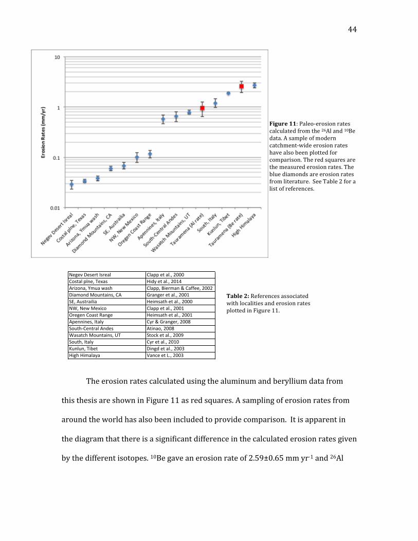
Figure 11…………………………………………………………………………………………………………...44
Figure 12…………………………………………………………………………………………………………...46
Figure 13………………………………………………………………………………………………………...…47
Figure 14…………………………………………………………………………………………………………...48
List of Tables
Table 1………………………………………………………………………………………………………………39
Table 2………………………………………………………………………………………………………………44

v
Acknowledgments
First I would like to thank John Gosse for all of the guidance and support he provided over the course of my thesis. His enthusiasm and positive attitude kept me hard at work even at the most difficult of times. I have learned so much from him during our weekly meetings (and not just about my thesis).
I need to thank Guang Yang for all of her help with the chemistry. Her tutelage in the lab was invaluable, and without her help this thesis could never have been finished on time. Thanks to Martin Gibling for all of his help in preparing my thesis and keeping me on tract. Also thanks to Mike Taylor and Gabriel Veloza Fajardo who did the hard work by going to Columbia and collecting the samples. Thanks to Alan Hidy and Susan Zimmerman who managed to get great AMS measurements from my difficult samples. And of course many thanks to all of my friends and family, who provided invaluable support. The fact that they took the time to try and understand cosmogenic isotopes so that they could listen to me talk about about my thesis meant a lot.

1
1.0 Introduction
Terrestrial cosmogenic nuclide (TCN) burial dating is a powerful tool used in
many different situations to develop a better understanding of the geology of a
region. This thesis will focus on the 26Al/10Be system in quartz. This burial dating
method has a wide range of applications and has been used to date alluvial fan
surfaces, terraces and lava flows, to name a few examples (Granger & Muzikar,
2001). Burial dating has also been used to date strain markers, which can be used to
determine the deformation history and develop a tectonic interpretation for a
region (Gosse & Phillips, 2001).
The strength of TCN burial dating is that it can be used where other methods
cannot. For sediments older than 50 ka and 1.5 Ma, respectively, radiocarbon and
luminescence dating are not viable (Blaco & Rovey, 2008). Sediments of Pliocene-‐
Pleistocene age can be dated with U-‐series or tephrochronology only in rare
instances where suitable material is available in a useful stratigraphic sequence
(Balco & Rovey, 2010). While there are limitations to the application of TCN burial
dating, the technique can be used on a variety of different isotope-‐mineral systems
(e.g. 26Al and 10Be in quartz) and a broad age range from 103 years with a short-‐lived
isotope, to 107 years with a long lived isotope (Gosse & Phillips, 2001).
The most significant weakness of cosmogenic burial dating is that an
assumption about the value of the initial 26Al/10Be ratio for a sample must be made
(Hidy, 2013). In order to calculate an age, the initial ratio of 26Al to 10Be must be
known (Balco & Rovey, 2010). This is very difficult where sediment is involved.
Sediment, which has been eroded from a source, has an unknown inheritance of 26Al
2
and 10Be (Balco & Rovey, 2010). It is impossible to measure the initial ratio of 26Al
/10Be in these situations so an assumption is made that the initial ratio of 26Al /10Be
in the sediment is equal to the surface production ratio for 26Al /10Be of 6.75 (Balco
& Rovey, 2008).
A TCN isochron burial dating method was first employed by Balco & Rovey,
(2008) to reduce the sensitivity of a burial age to the initial isotopic ratio.
Application of the isochron burial dating method requires samples from a depth
profile in the soil of a sediment package that was exposed prior to burial. If exposure
was sufficiently long (many thousands of years) significant in-‐situ production of
TCN in the quartz sand would have rendered any initial 10Be or 26Al inconsequential
(Balco & Rovey, 2008). The isochron of interest is the slope of the ratio of two
isotopic concentrations. The slope of 26Al /10Be isochron (which is actually a curve
owing to the fact that their production rates and decay rates are different) is best
defined if there is a significant range of 26Al and 10Be among different samples at the
site. Such a range can be achieved by analyzing multiple samples in a depth profile,
because the cosmic rays are absorbed as they interact with mass. Thus, the samples
near the top of a buried profile can have an order of magnitude higher
concentrations than those at the bottom (Balco & Rovey, 2008). However, this
variation of 26Al and 10Be concentration with depth only develops when the surface
has been exposed for a long enough period of time (Balco & Rovey, 2010). Sampling
is often done within paleosols as these are indicative of surfaces that have
experienced a long period of exposure.

3
There is another option for sampling related samples with a range of 26Al and
10Be concentrations. In locations where cobbles are present it is possible that the
concentration of 26Al and 10Be in each cobble would be sufficiently different (i.e. if
they were exhumed from different depths just prior to deposition) to define an
isochron. This experiment has been recently conducted and shown that the scatter
is sufficient (Balco et al., 2013).
However, in many locations there are no paleosols to sample for burial
dating of sediments or the fluvial sediments are sufficiently fine grained that no
cobbles are present (e.g. on coastal plains such as the Pliocene Beaufort Fm at
Beaver Pond Site, Ellesmere Island, Canada; Rybczynski et al, 2013). In such cases, a
different method is needed for cosmogenic burial dating. This thesis proposes one
such method.
The measurement of TCN in different grain size fractions in sediment from
steeply sloped catchments, which are prone to landslide, should provide sufficient
range in the TCN concentrations to define an isochron. This strategy makes use of
the fact that depth profiles exist in catchments, and that mass wasting events can
sample them, as opposed to surface runoff which would just sample the uppermost
regolith-‐bearing sediment with more uniform concentrations of TCN. The upper
part of the surface has been more weathered so it will break up into finer grained
sediment, while deeper material will remain coarser grained.
The upper part of the surface was also exposed to more cosmic rays, so it will
have higher concentrations of cosmogenic nuclides than the deeper sediment. It
may be possible to use this nuclide concentration covariance with grain size instead
4
of a depth profile in the isochron dating method, eliminating the need to find a
paleosol. In order to properly sample these profiles we would need the landslides to
go to a mass depth of 1 m/g2 below the surface.
Many previous studies have documented a TCN concentration variation with
grain size while studying erosion rates for Pliocene and early Quaternary sediments
in active orogens (Atinao, 2008; Belmont, 2007; Brown et al., 1996; Puchol et al.,
2014; Veloza et al., unpub.). These studies were done in regions of high relief and it
is believed this phenomenon can be attributed to the effect of deep-‐seated land
sliding (Brown et al, 1996).
However, regions of high relief often have very rapid erosion rates, in part
because of the landsliding and other accelerated hillslope processes. Increased
erosion results in a decrease in the concentration of cosmogenic isotopes in
sediment due to the deeper, lesser-‐exposed sediment being brought to surface.
Therefore this thesis also proposes the idea that a grain-‐size dependent isochron
method will not be able to be resolved, due to the decreased TCN concentrations
resulting from rapid erosion in the catchment of high relief areas.
To reiterate, in this thesis two hypotheses will be tested: (H1) That the
isochron method can be done using different grain size fractions, in regions prone to
shallow landsliding and alternatively, (H2) that the high erosion rates associated
with the catchments of regions with high relief will result in a decrease of TCN
concentrations to the point where it will not be possible to get accurate enough
measurements to define an isochron.

5
In this thesis the theory behind the grain-‐size dependent isochron method
will be presented and a field test will be applied in the Tauramena locality of the
Colombian Andes. This location is an ideal test site because (i) preliminary ages
have already been done using a 26Al /10Be simple burial dating method indicate
minimum ages of 2.5 Ma (Veloza et al., unpub), which gives us an idea of what to
expect; (ii) the Guayabo Fm comprises alluvial fan and fluvial terrace deposits at the
mountain front of a high relief tectonically active origin where small landslides are
common; (iii) a grain-‐size dependence has already been revealed in the Cordillera
Principal of the Southern Central Andes (Antinao, 2008), suggesting that the same
relationship may exist in the Colombian Andes; and (iv) the exact timing of the
Guayabo Fm. is of significance because it may record a significant change in
sediment flux at the Plio-‐Pleistocene boundary (2.6 Ma).
If this method proves functional, then it can be applied to other terrains with
steep slopes where landslides or other mass wasting processes occur, which cause
the erosion and deposition of subsurface regolith. For example Puchol et al. (2014)
studied this phenomenon in a drainage basin in the central Himalayas and Belmont
et al. (2007) noted this in Washington State.

6
2.0 Background and geologic setting
2.1 TCN dating principles
TCN methods use the production of particular nuclides in minerals from
interactions of their atoms with cosmic rays (Granger & Muzikar, 2001). Cosmic
rays are particles such as protons and muons that come from space and enter our
atmosphere. TCN dating exclusively considers particles that originate outside of our
solar system and which form primarily during supernova events (Gosse & Phillips,
2001). The flux of these particles to Earth is considered constant over the time
periods for which TCN dating can be applied. However, the flux that reaches the
surface of the Earth is altered significantly by the strength of the magnetic field,
which varies spatially and temporally (Gosse & Phillips, 2001).
Interactions of cosmic rays with atoms in the atmosphere result in the
production of secondary particles. These new particles may then collide with other
atoms, creating more particles, resulting in a cascade effect, or cosmic ray shower.
After an average of ten disintegrations, the secondary particles eventually make it to
the surface of the Earth where they interact with atoms in minerals to create new
nuclides (Granger & Muzikar, 2001). The depth to which the particles penetrate
depends on their probability of interaction (or nuclear cross section), which is
mainly a function of their energy, size, and charge (Gosse & Phillips 2001).
Many different nuclides are created, some of which are useful for
geochronology and erosion rate applications, depending on decay rates and the

7
Figure 1: The production of 10Be and 26Al in quartz at sea level and high latitude by spallation and muon interactions. A. Plot showing the build up of 26Al and 10Be in quartz over time. 26Al is produced from 28Si at a faster rate (higher cross section) than 10Be from 16O and 28Si combined. Both nuclides eventually reach saturation, however the shorter-‐lived 26Al reaches this point first. The dashed lines show how erosion rates of 0.1, 0.3, and 1.0 cm/kyr lower the concentration measured in the surface, and accelerate the saturation of each radionuclide. The bolded solid line shows the change in the 26Al/10Be ratio with time. These are based on production rates and decay constants that were used in 2001. Since then there have been updates to both. B. A 26Al /10Be vs. 10Be plot (the zero-‐erosion scenario is represented by the thick, solid line). The thin lines with triangles show how the ratio of 26Al /10Be would be affected by a given erosion rate. Samples that plot on the solid thick line provide an exact exposure age using both nuclides, and there is no indication of burial or erosion of the surface. Samples that plot in the banana-‐shaped field represent surfaces that have been exposed and eroded. Samples plotting below the banana indicate that the surface was exposed, and then completely or partially buried at least once (production was slowed or halted but decay continued, so the ratio decreased by an amount proportional with the burial duration). Figure from Gosse & Phillips, 2001.
abundance of the isotopes produced by non-‐cosmogenic pathways (radiogenic or
nucleogenic). For example 26Al and 10Be, which are formed primarily by spallation,
and have relatively small non-‐cosmogenic abundances, are both useful nuclides for
calculating ages through the Pleistocene (Gosse & Phillips, 2001). 26Al and 10Be have
half-‐lives of 0.705 Ma and 1.39 Ma, respectively (Balco & Rovey, 2011).
Surface exposure dating
TNC are commonly used to determine how long a surface has been exposed
above ground (Gosse & Phillips, 2001). 26Al and 10Be nuclides are ideal for this
method because they are both relatively immobile, form in quartz (which is the
most abundant mineral in the continental crust), and have different half-‐lives and
production rates (Gosse & Phillips, 2001).
8
The idea behind surface exposure dating is that as long as a surface is
exposed it will be bombarded by cosmic rays and TCN will be produced. 26Al is
produced more quickly than 10Be, however the exact production rates vary
depending on several factors such as latitude, altitude and shielding (Gosse &
Phillips, 2001). The longer the surface is exposed the higher the concentration of
TCN. Both of these radionuclides decay so eventually they will reach a saturation
point, where production rate is equal to decay rate and their concentrations remain
constant in the rock (Gosse & Phillips, 2001). 26Al has a higher production rate and
shorter half-‐life so it reaches its saturation point before 10Be, as shown in Figure 1a.
Due to the characteristics of these nuclides, their ratio changes significantly
with time, as represented by the bold line in Figure 1b. Erosion of the surface will
result in a decrease in the concentrations of 26Al and 10Be, since erosion will advect
previously partly shielded minerals toward the surface. The thinner lines with
triangles in Figure 1b represent the effect of variable erosion rates on the ratio of
26Al /10Be. Surface exposure dating can be applied to surfaces of bedrock landforms
(e.g. fault scarp, lava, or tor) or sediment landforms (e.g. terrace, fan, landslide).
Simple burial dating.
It is often useful to determine when a buried surface, such as a buried soil or
peat, became shielded by other sediment, lava, or even water. This can be done with
TCN burial dating. The ideal situation for this method is when the surface of interest
was exposed for a long time (>103 years) and then is instantaneously buried,
resulting in a complete stop in the flux of cosmic rays to the surface (Lal, 1991). In

9
other words, after burial there is no more production of cosmogenic nuclides but
the 26Al/10Be ratio continues to decrease owing to differences in the decay rates of
the isotopes (Fig. 1a,b). The decrease is proportional with burial time. If only one
complete burial event has occurred, then the exact burial duration can be calculated
(shown graphically in Fig. 2). In reality however, the situation is rarely ideal with
complexities that must be taken into account, such as slow burial, re-‐exposure of the
surface, and production of nuclides by deep-‐penetrating muons (Granger & Muzikar,
2001). To simplify calculations certain assumptions have to be made.
Since the half-‐lives of 26Al and 10Be are known, as is their production ratio, it
is possible for us calculate how the ratio of 26Al/10Be would change through time in
a buried surface. A burial duration is computed for a measured 26Al/10Be ratio (Fig.
2; Granger & Muzikar, 2001).
The simple burial dating method requires the assumptions that (i) the initial
ratio of 26Al/10Be was 6.75 (i.e. that there was only one burial event and, in the case
Figure 2: Burial plot for 26Al/10Be. It represents the 26Al/10Be ratio in sediment over time. The topmost dashed line represents the change in the 26Al/10Be ratio in a surface with constant exposure (equivalent to the solid thick line of Fig. 1b). The topmost solid line represents the exposure time of a surface undergoing a range of steady erosion (as indicated by the dashed lines) but no burial. As soon as burial occurs, radioactive decay will control the 26Al/10Be ratio. The 26Al and 10Be ratios indicate burial duration, as indicated by the other solid curves which correspond to longer and longer burial age with decreasing ratio. Production rates and decay constants are as per 2001. Figure from Granger & Muzikar, 2001.

10
of dating sediments, there was no prolonged sediment storage prior to the final
deposition of the sediment) and (ii) that there was no post-‐burial muonic
production. In other words, it was assumed that a single simple burial occurred.
This assumption is the biggest weakness of TCN burial dating (Hidy, 2013).
The model for burial dating is that of a surface in a catchment area building
up 26Al and 10Be at a ratio of 6.75 26Al atoms for every 10Be atom (the production
ratio was 6.1 in 2001, Fig. 1a,b; Fig. 2), and then the surface being eroded and
immediately buried. If buried sediment in the real world does not actually follow
this model, our assumption of the initial ratio of 6.75 is incorrect. If the ratio at the
time of deposition was less, then the simple burial age will over-‐estimate the actual
duration of the last burial event. In reality, by using the simple burial dating method
we are calculating a maximum burial age (Balco & Rovey, 2010).
Depth profile isochron method.
To resolve this issue, isochron burial dating was developed. The premise of this
method is to avoid the assumption of an initial ratio of 6.75 by sampling in a manner
that circumvents the need to make the assumption (Balco & Rovey, 2008). This can
be done by taking a depth profile below a previously exposed surface. It is well
documented that TCN concentrations decrease with depth (Lal, 1991). Sediment at a
landforms surface will have the maximum production of nuclides for a particular
layer. As depth increases, the sediment at depth becomes more shielded by the
sediment above. Fewer cosmic rays are able to penetrate to depth due to their
interactions with the sediment at surface.

11
This attenuation of the cosmic ray energy is predictable based on knowledge
of the secondary cosmic ray flux (particle energy, type) and nuclear cross sections
for their interactions with target minerals. This phenomenon is illustrated in Figure
3, below. Though the concentrations of 26Al and 10Be vary with depth through a
layer of sediment, the ratio of 26Al/10Be should be the same (at least in the upper 2
meters) through the entire sediment package since the total cosmic ray flux to the
sediment package was the same (Balco & Rovey, 2008). At greater depth, the greater
production of 26Al than 10Be by muons will change the ratio. So, by sampling within
the first 2 meters of a buried soil (200 cm in a sediment with bulk density of 2 g cm-‐3
is equivalent to a mass depth of 400 g cm-‐2, Fig. 3) a constant isochron can be
defined, whereby the slope of the 26Al /10Be curve is a function of burial duration
(Fig. 4).
Figure 3: Measured 26Al and 10Be concentrations below a paleosol. There is a clear decrease in concentration with depth, however the ratio of 26Al and 10Be remains the same. Note the y-‐axis is mass depth, a function of true depth and bulk density. Figure from Balco & Rovey, 2008.

12
The concept of the isochron plot is shown in Figure 4. By plotting the 26Al
concentrations against 10Be concentrations of several samples from different depths
in the same layer, it is possible to define a line. The slope of this line is the 26Al/10Be
ratio and can be used to calculate a burial age.
The line defined by the samples can then be compared to isochron lines
corresponding to a simple burial history. These isochron lines are calculated based
on the assumption that initial ratio of 26Al/10Be in the sample was 6.75 prior to
burial. This would be the case if almost all of the TCN concentrations were produced
in the depth profile. If the line defined by the measured data points fits onto or is
parallel to the isochron lines, then the initial ratio for the samples was 6.75. If the
slope of the measured points crosses the simple burial isochron lines, then the
assumption is incorrect meaning that the sediment has experienced a complex
burial history. The biggest weakness of the depth profile isochron method is that it
can only be applied in situations where a paleosurface was exposed for a long
period of time. The long exposure is what allows the gradient in 26Al and 10Be
Figure 4: An isochron burial plot. 26Al and 10Be concentrations in quartz are plotted against each other. Points represent hypothetical samples from different depths from the same package of sediment. The points will define a line, the slope of which is the 26Al/10Be ratio for the package of sediment. This ratio can then be used to calculate a burial age. The thick dark lines and points represent the change in slope that occurs with increased burial time for hypothetical data. As time after burial progresses the slope of the line will become less steep as both isotopes decay. The thin solid line represents a surface with constant exposure. The thin dotted lines are isochrones. They are the calculated ratio of 26Al and 10Be in the constant exposure surface after a set burial time. Figure from Balco & Rovey, 2008.

13
concentrations with depth to develop. If the period of exposure is not long enough,
no gradient will develop and the method cannot be applied (Rybcynski et al., 2013).
The isochron method has also been done by collecting several cobbles from
the same layer in a sediment deposit, instead of using a depth profile (Balco et al.,
2013). The idea is that these large clasts probably originated from different parts of
the catchment area before being buried together. This means each clast has come
from a different location and has a slightly different history. This results in
variations in the production rates of TCNs and erosion rates experienced by the
clasts, which ultimately results in each individual clast having a different
concentration of 26Al and 10Be (Balco et al., 2013). However, since all of the clasts
came from the same catchment (should have the same initial 26Al/10Be ratio), and
were all buried for the same amount of time (all experienced the same amount of
decay), then they should have the same 26Al/10Be ratio. Since the cobbles should
have the same ratio and should have various 26Al and 10Be concentrations, they can
be used to define an isochron, from which a burial age can be calculated (as
previously explained). The biggest weakness of this method, given that a sufficient
number of cobbles are present at the sample site, is that the initial ratio of the
cobbles must be assumed to be 6.75, and one must hope that the cobbles chosen
during sampling have enough variation in TCN concentration to define an isochron.
14
Grain size isochron method.
In regions of high relief, which are frequented by landslides, it may be
possible to avoid having to find a paleosol in order to apply the depth profile
isochron method. In several cases in regions of high relief, where landslides are
common, a variation in the concentration of TCNs with grain size has been observed
(Brown et al., 1996; Belmont et al., 2007; Antinao, 2008; Puchol et al., 2014). For
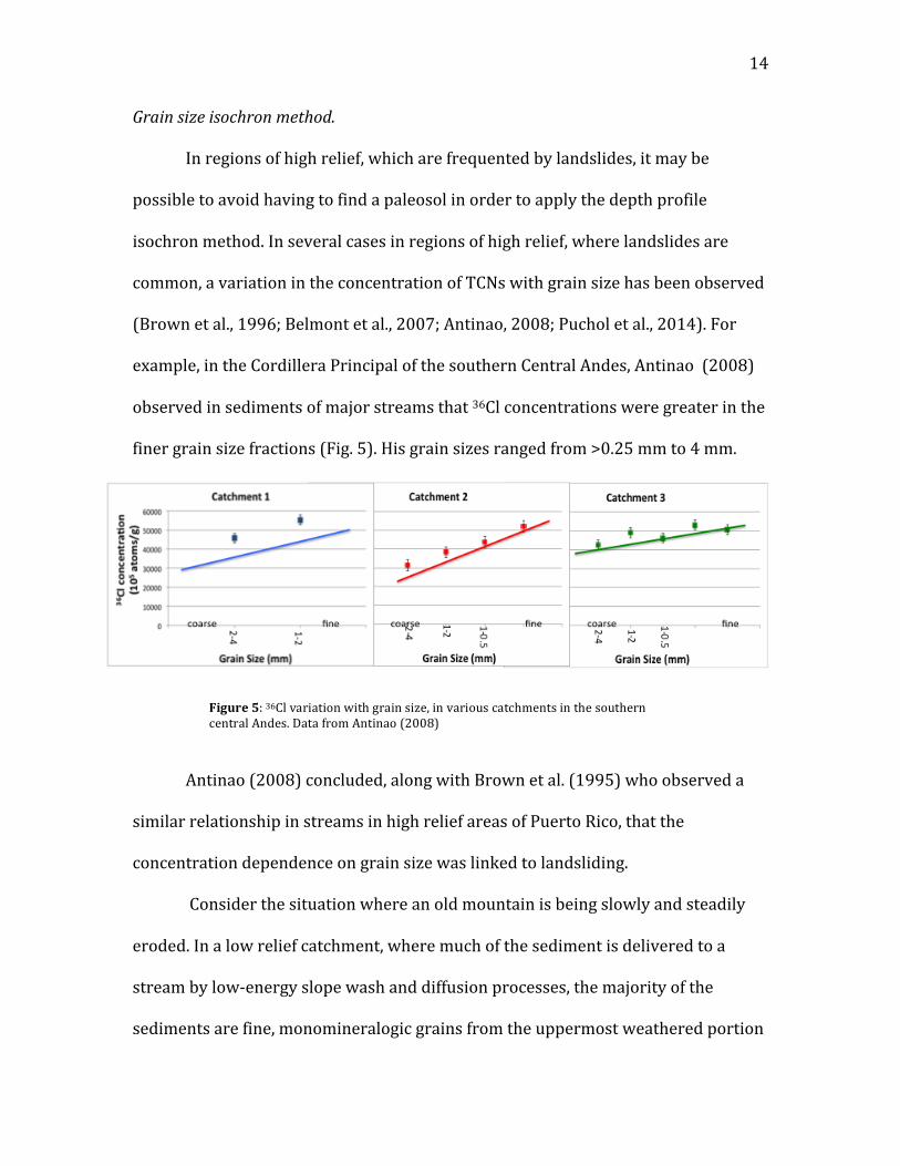
example, in the Cordillera Principal of the southern Central Andes, Antinao (2008)
observed in sediments of major streams that 36Cl concentrations were greater in the
finer grain size fractions (Fig. 5). His grain sizes ranged from >0.25 mm to 4 mm.
Antinao (2008) concluded, along with Brown et al. (1995) who observed a
similar relationship in streams in high relief areas of Puerto Rico, that the
concentration dependence on grain size was linked to landsliding.
Consider the situation where an old mountain is being slowly and steadily
eroded. In a low relief catchment, where much of the sediment is delivered to a
stream by low-‐energy slope wash and diffusion processes, the majority of the
sediments are fine, monomineralogic grains from the uppermost weathered portion
Figure 5: 36Cl variation with grain size, in various catchments in the southern central Andes. Data from Antinao (2008)

15
of regolith. On the other hand, in an active orogen, where slopes are steeper than
26°, a large portion of the sediment may be delivered by mass wasting processes
(Antinao, 2008). The sediment delivered to the stream by mass wasting will
comprise both the finer weathered material from the top of the weathered regolith,
but also some larger, less weathered, multi-‐mineralogic fragments that are less
easily comminuted in the short transport time. The finer grain sizes, being closer to
the surface, experienced a higher cosmic ray flux resulting in more 26Al and 10Be
production, whereas the coarser stream sediments were deeper and more shielded
from cosmic rays, hence the grain size dependency. On average the sediment is
derived from a few meters of regolith, which like the depth profile method, provides
enough spread in the concentrations between the fine and coarse fractions to define
an isochron (cf. Fig. 4 and Fig. 5), but the 26Al/10Be ratio through it should be
approximately constant at 6.75. Using this method it should be possible to construct
an isochron plot, but instead of using a depth profile that formed in a buried
paleosol, this approach uses different grain sizes from a depth profile that formed in
a mass-‐wasted regolith.

16 c
0
-20
-40
-60-80 -40
-726
6
Structure axis and plungedirectionThrust
N
Tear fault cZamaricotesyncline
Yopal Fault
Corozalantincline
Tameantincline
20 km
Paz de AriporoFault
-76 -72
2
6
10
200 km
WWCCCCCC
EECC
N
CCBB
NNZZ
a
SouthAmerica
b
Figure 1
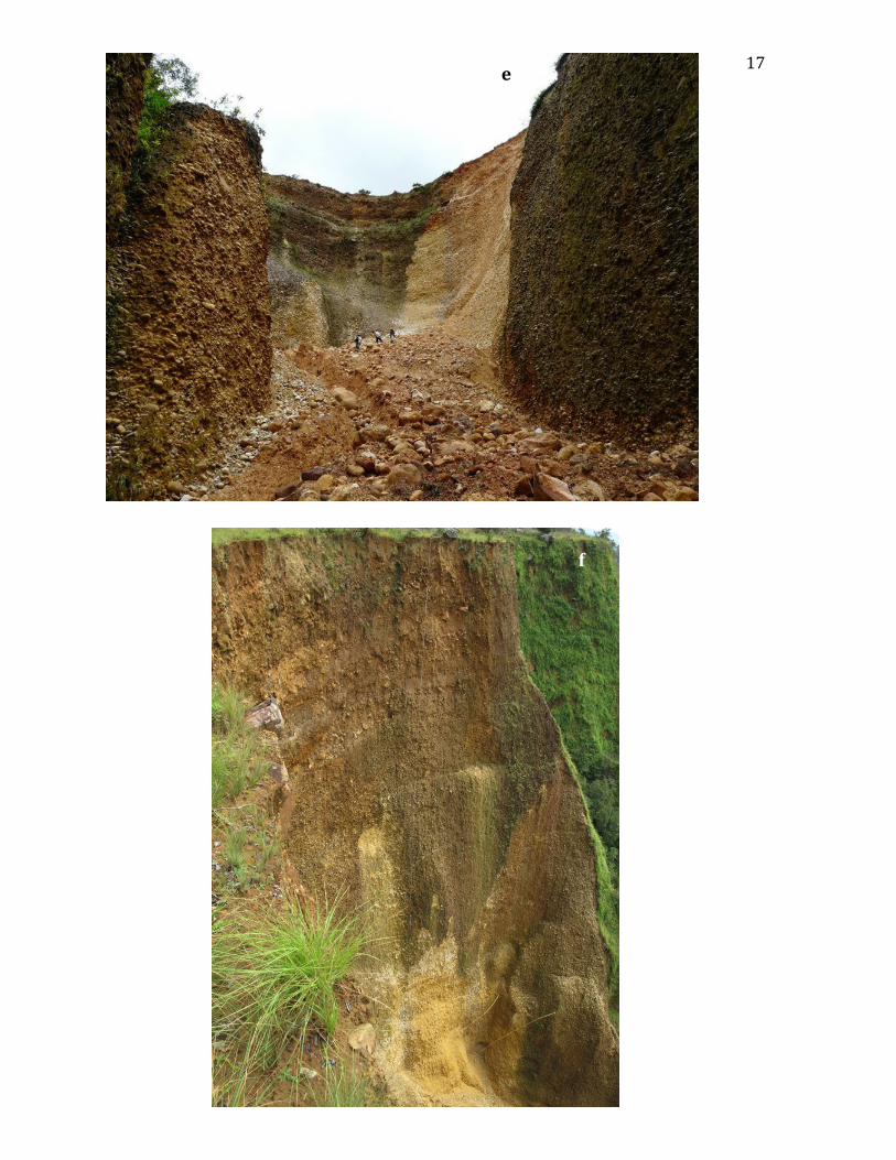
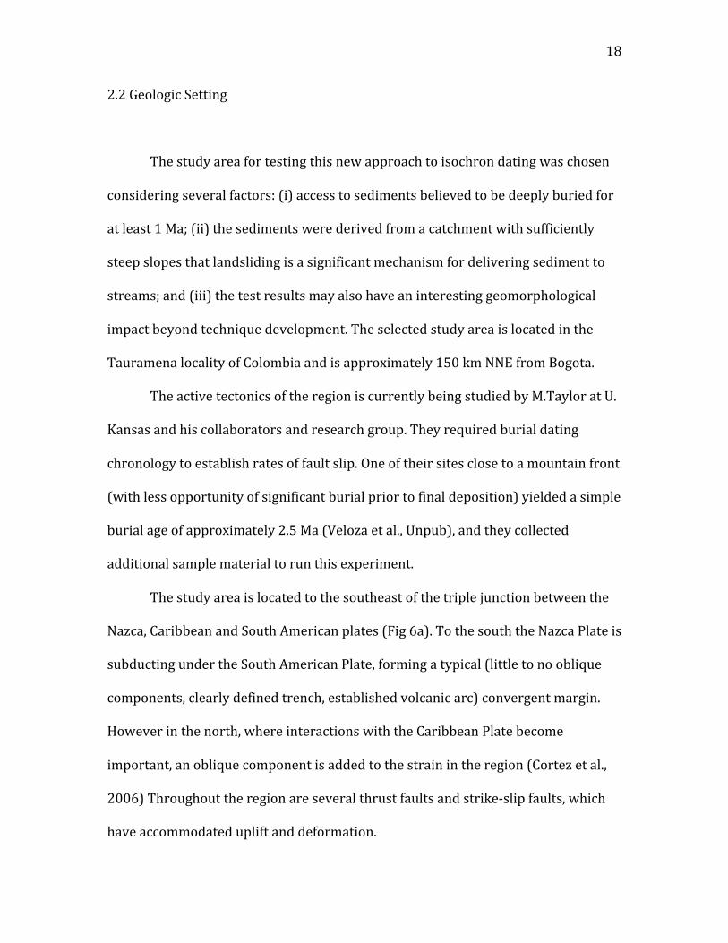
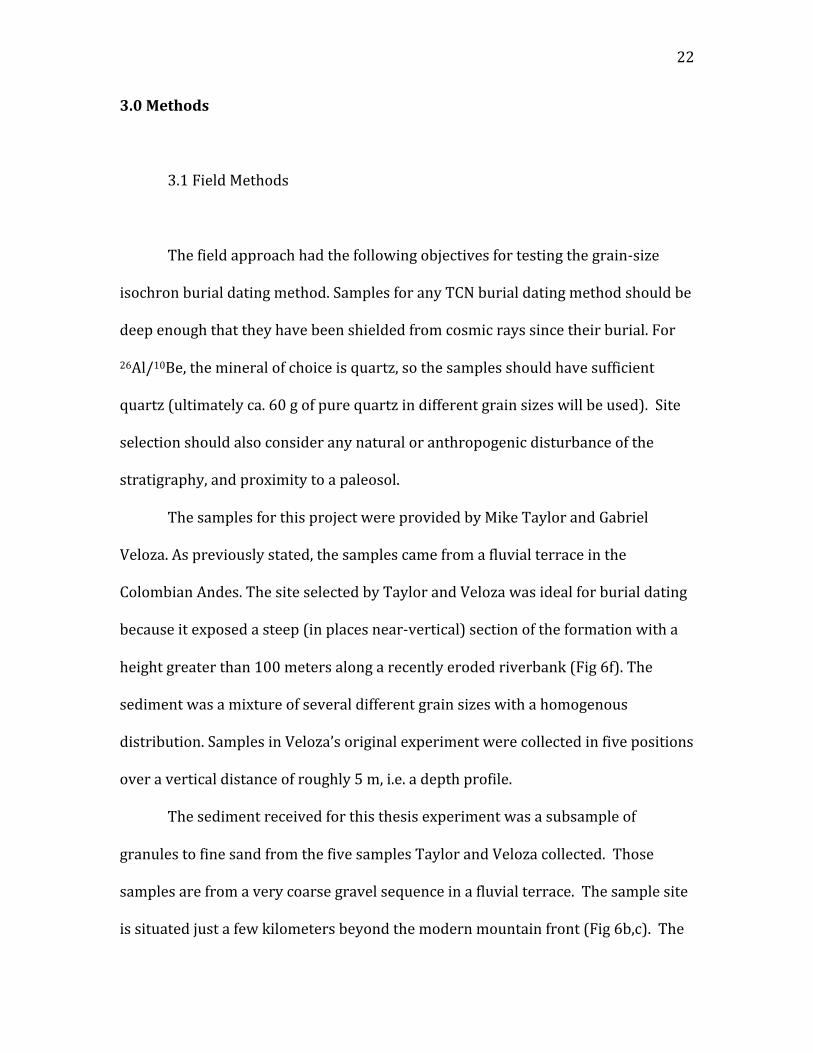
Figure 6: A. Map of South America, showing where the sample site (blue rectangle) is located. Figure modified from Veloza et al, (unpub). B. Regional map of the Colombian Andes. CB is the Caribbean Plate, NZ is the Nazca Plate and SA is the South American Plate. WC is the Western Cordillera, CC is the Central Cordillera and EC is the Eastern Cordillera. The green rectangle represents the sample site. Figure modified from Veloza et al, (unpub). C. Over view of the sediment deposit for this thesis. The yellow arrow shows the sample site. Image from Google Earth. D. Image showing proximity of the sample site to the mountain front and landslides. Image from Google Earth. E. (Below) Sediment of the Guayabo Fm at the sample site. Photo from Mike Taylor. F. (Below) Samples were taken from the base of this cliff face. The cliff has a height of 112m. Photo from Mike Taylor.
d
17
f
e
18
2.2 Geologic Setting
The study area for testing this new approach to isochron dating was chosen
considering several factors: (i) access to sediments believed to be deeply buried for
at least 1 Ma; (ii) the sediments were derived from a catchment with sufficiently
steep slopes that landsliding is a significant mechanism for delivering sediment to
streams; and (iii) the test results may also have an interesting geomorphological
impact beyond technique development. The selected study area is located in the
Tauramena locality of Colombia and is approximately 150 km NNE from Bogota.
The active tectonics of the region is currently being studied by M.Taylor at U.
Kansas and his collaborators and research group. They required burial dating
chronology to establish rates of fault slip. One of their sites close to a mountain front
(with less opportunity of significant burial prior to final deposition) yielded a simple
burial age of approximately 2.5 Ma (Veloza et al., Unpub), and they collected
additional sample material to run this experiment.
The study area is located to the southeast of the triple junction between the
Nazca, Caribbean and South American plates (Fig 6a). To the south the Nazca Plate is
subducting under the South American Plate, forming a typical (little to no oblique
components, clearly defined trench, established volcanic arc) convergent margin.
However in the north, where interactions with the Caribbean Plate become
important, an oblique component is added to the strain in the region (Cortez et al.,
2006) Throughout the region are several thrust faults and strike-‐slip faults, which
have accommodated uplift and deformation.

19
The Colombian Andes comprise three separate mountain chains, the Western
Cordillera (Occidental), the Central Cordillera and Eastern Cordillera (Oriental) (Fig.
6b). The Western Cordillera is composed of layers of Cretaceous accreted sediment,
separated by late Cenozoic aged thrust faults that verge roughly north-‐west (Cortes
et al., 2006; Veloza, 2012). The Central Cordillera is an active volcanic arc, which
was active since the Miocene. The Eastern Cordillera is a modern fold-‐and-‐thrust
belt that formed from the structural inversion of a Cretaceous back-‐arc basin
(Cortes et al., 2006; Gregory-‐Wodzicki, 2000). The inversion resulted in the
conversion of normal faults to reverse faults and occurred in the Eocene (Cortes et
al., 2006). This inversion was caused by a change in the stress regime from
extension and transtension to a compressive regime that caused episodic uplift that
continued to recent time (Cortes et al., 2006).
The study area is located on the eastern flank of the Eastern Cordillera (Fig.
6b,c,d). As previously stated, the region in which the sample site is located has been
undergoing uplift since the Eocene. The sample site itself is a fluvial terrace
composed of coble braided stream deposits (Fig. 6c). Due to its proximity to the
mountain front it probably has a significant component of sediment derived from
alluvial fans, however from the roundness and sorting of the sediment we can
determine that the bulk of it is of fluvial origin. The sediment package is classified as
part of the Upper Guayabo Formation, and is essentially a mixture of well-‐sorted,
very coarse alluvial gravel and braided stream sediments (Parra et al., 2010) (Fig.
6e). The deposited gravel appears to exhibit horizontal bedding, imbrication, and
good sorting (for a cobble gravel) which are consistent with their being fluvially

20
deposited, as opposed to deposition by debris flows or other gravity driven
processes. Based on the range of clast roundness (Fig. 6e, from very rounded to
subangular) some of the sediment has been transported in the stream for a long
distance, but some of the sediment was deposited after a short transport distance.
While it is possible that there may even be debris flows in this section, Taylor
indicates that this was not observed but also that the sedimentology was not
thoroughly examined.
The regional descriptions of the formation from literature describe it as a mix
of channelized sandstones and conglomerates (braided channel deposits),
horizontally stratified pebble to cobble conglomerates (alluvial fan deposits) and
poorly stratified cobble to boulder conglomerates (debris flow deposits) (Parra et al,
2010). The sample site is in close proximity to shallow landslides that occur in the
nearby mountains (Fig. 6d). These landslides are inferred to be a significant enough
source of sediment that their TCN signature can be distinguished among all of the
other processes that sourced sediment to the deposit.
A depth profile isochron burial age was attempted at the location in 2013 by
Veloza et al, (unpub). Six samples were submitted for 26Al/10Be analyses at a US
laboratory, however only four samples had a sufficient number of aluminum atoms
to obtain 26Al measurements, and the measurement precisions ranged from 57% to
143%. After blank subtraction, two of those samples yielded unacceptable results.
The remaining two samples had 1-‐sigma 26Al precisions of 57% and 70%, which was
insufficient to obtain a depth profile isochron burial age. However, the simple burial
ages (maxima) were calculated (Fig. 7) to be 2.65 ± 0.7 Ma and 2.25 ± 0.6 Ma. The
21
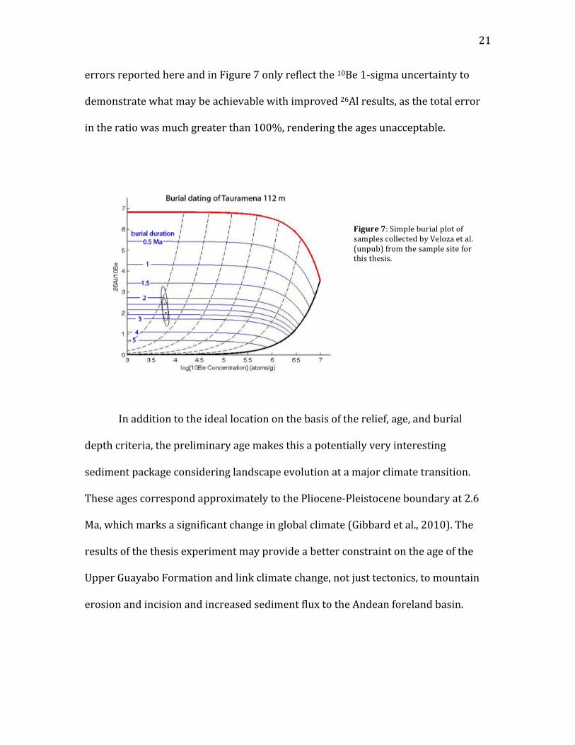
errors reported here and in Figure 7 only reflect the 10Be 1-‐sigma uncertainty to
demonstrate what may be achievable with improved 26Al results, as the total error
in the ratio was much greater than 100%, rendering the ages unacceptable.
In addition to the ideal location on the basis of the relief, age, and burial
depth criteria, the preliminary age makes this a potentially very interesting
sediment package considering landscape evolution at a major climate transition.
These ages correspond approximately to the Pliocene-‐Pleistocene boundary at 2.6
Ma, which marks a significant change in global climate (Gibbard et al., 2010). The
results of the thesis experiment may provide a better constraint on the age of the
Upper Guayabo Formation and link climate change, not just tectonics, to mountain
erosion and incision and increased sediment flux to the Andean foreland basin.
Figure 7: Simple burial plot of samples collected by Veloza et al. (unpub) from the sample site for this thesis.
22
3.0 Methods
3.1 Field Methods
The field approach had the following objectives for testing the grain-‐size
isochron burial dating method. Samples for any TCN burial dating method should be
deep enough that they have been shielded from cosmic rays since their burial. For
26Al/10Be, the mineral of choice is quartz, so the samples should have sufficient
quartz (ultimately ca. 60 g of pure quartz in different grain sizes will be used). Site
selection should also consider any natural or anthropogenic disturbance of the
stratigraphy, and proximity to a paleosol.
The samples for this project were provided by Mike Taylor and Gabriel
Veloza. As previously stated, the samples came from a fluvial terrace in the
Colombian Andes. The site selected by Taylor and Veloza was ideal for burial dating
because it exposed a steep (in places near-‐vertical) section of the formation with a
height greater than 100 meters along a recently eroded riverbank (Fig 6f). The
sediment was a mixture of several different grain sizes with a homogenous
distribution. Samples in Veloza’s original experiment were collected in five positions
over a vertical distance of roughly 5 m, i.e. a depth profile.
The sediment received for this thesis experiment was a subsample of
granules to fine sand from the five samples Taylor and Veloza collected. Those
samples are from a very coarse gravel sequence in a fluvial terrace. The sample site
is situated just a few kilometers beyond the modern mountain front (Fig 6b,c). The

23
samples were collected near the base of a deep gully that exposes over 112 m of the
gravel above the modern stream (Fig 6f).
As previously mentioned, due to the wide range of grain size and roundness
of the clasts it is likely that the sediment in the deposit originally was formed in a
variety of processes before being transported and deposited by a fluvial system.
Having sediment delivered to the mainstem stream from a wide range of surface
processes will help produce a wider scatter in the TCN concentrations among
different samples, and a wide concentration range is needed to more precisely
define an isochron slope (if all of sediment had exactly the same concentration, i.e.
each bag was a perfect mixture of a homogeneous population) then no isochron
slope can be defined.
The biggest issue for collecting samples for burial dating is that the shielding
of the samples must be taken into account. The amount of shielding will affect the
amount of post-‐burial production of 26Al and 10Be (Gosse & Phillips, 2001). Post-‐
burial production is due to spallation by neutrons and muons (Balco & Rovey,
2008). By blocking the flux of these cosmic rays, shielding decreases post-‐burial
production. There are two major considerations when calculating the amount of
shielding a site has. The first is the topography of the area, which takes into
consideration how exposed the sample site is and whether any topographic features
such as nearby mountains could block cosmic ray flux. The second consideration is
the depth to which the sample is buried. All cosmic particles have an attenuation
length, meaning that by increasing the depth of a sample, the flux of cosmic rays to
the sample decreases (Gosse & Phillips, 2001).

24
For this particular project, shielding is not an issue for the samples since they
were buried by more than 100 meters of sediment (Fig 6f). This thick sediment
layer completely shielded the samples from cosmic rays meaning there would be
negligible post-‐burial production. The only way that production may have occurred
is by cosmic rays entering at shallow angles onto the steep face. However, because
the cosmic ray flux is angular dependent (85% of the particles enter within a
vertical 45° cone), the sample site was actually in a deeply and actively incising
gulley cut into the river bank, and the sampled zones were cleaned (minimum 20
cm) before collecting the samples, post-‐burial production is considered very
unlikely (Lal, 1991). Measurement of in situ cosmogenic 14C in the samples would
test this assumption.
The five ca. 3-‐kg samples with grain sizes ranging from pebbles to silt were
collected with spades from six shallow pits in the section face 112.5 meters below
the top of the sediment package and stored in triple-‐labeled double ziplock bags.
While the depth profile method requires five samples collected in a vertical
sequence, the samples for the grain size isochron method can be collected from a
single thin layer, or, considering the precision of the technique will be greater than
104 years, we could amalgamate samples over a 2 meter or thicker layer.
25
3.2 Lab methods
3.2.1 Physical Processing.
All processing for the grain size isochron burial dating method test was done
using the facilities at the Dalhousie Geochronology Centre. Different grain size
fractions were separated with a sieve shaker and 8” stainless steel sieves. Originally
it was hoped that each sample would have its own set of TCN samples with distinct
grain sizes. However there was a lack in quartz mass in certain grain sizes for
particular samples, meaning that in order to be able to run the samples, the
sediment remaining from all five pits had to be combined. The initial size fractions
were >8, 8-‐4, 4-‐2, 2-‐1, 1-‐0.85, 0.85-‐0.5, 0.5-‐0.355, 0.355-‐0.250, 0.25-‐0.15 mm, but it
was anticipated that two or more of these fractions may need to be combined in
order to obtain 60 g of pure quartz for each grain size fraction.
Before chemical processing could begin the all of different grain size
fractions had to be crushed to the same grain size, which would also optimize
chemical dissolution. A fine grain size is not desirable because it increases the rate
at which dissolution in hydrofluoric acid (HF) occurs, making it more likely that too
much quartz will be undesirably dissolved. However the sample has to be fine
enough that each grain is a single mineral phase. For this project the optimum grain
size, considering that the limited lab time required aggressive use of HF, was 0.355-‐
0.250mm. Grain sizes smaller than 0.355-‐0.250 mm were not physically processed.
The coarser grain size fractions were put through a jaw crusher and all of the grain

26
size fractions were put through a disk mill in order to reduce them to the optimum
grain size.
3.2.2 Chemical Processing.
After each grain size fraction was reduced to the selected grain size, mineral
separation and quartz purification began. The goal of chemical processing is to the
isolate the quartz fraction for each sample without losing much quartz. Typical
quartz efficiencies are 40%, including a step that intentionally dissolves 35% of the
quartz to remove any meteoric 10Be (Kohl & Nishiizumi, 1992). First the samples
were boiled in aqua regia. This dissolved weaker minerals such as micas and
removed many of the metals. Next the samples were briefly exposed to hydrofluoric
acid to weaken the silicate phases in the samples.
The bulk of the dissolution of non-‐quartz phases was done in the next step
where the samples were split up into small bottles that were then filled with
hexafluorosilicic acid (F6 acid). Because of its ability to break Al-‐O bonds but not Si-‐
O bonds, this acid dissolves non-‐quartz silicates, and leaves quartz relatively
unaffected (Rees-‐Jones, 1995). This was the first time that F6 acid was used in a
systematic way in the DGC cosmogenic lab, and therefore as part of this thesis
research a series of tests was designed to optimize the efficiency of the dissolution.
The F6 optimization tests involved varying the mass of sample between 10-‐30 g and
the volume of acid, pretreating the samples with concentrated HF, and heating the
bottles at different temperatures. A hot dog roller was purchased to constantly mix
the samples and keep them at an optimum temperature. The optimum procedure
was to place 20 g of sediment, boiled in concentrated (46%) HF for 20 minutes, into

27
a 250 ml HDPE bottle with 50 ml of F6, on the hot dog roller with temperature
setting approximately 60°C. Care needed to be taken to ensure the caps were
securely fastened, that the bottles were each vigorously shaken by hand at least
once each day, and that pressure was released daily by briefly loosening the cap.
This F6 procedure lasted for weeks for each sample and because such large masses
of pure quartz were needed to ensure sufficient 10Be and 26Al precision, many
samples had to be split into different containers to speed dissolution.
Following this the samples were exposed to dilute hydrofluoric acid and
placed in ultrasonic tanks for aggressive dissolution of the quartz. The ultrasonic
tanks heated the samples to 95°C and sped up the dissolution process significantly.
The goal of this step was to dissolve the outer part of the quartz grains, to ensure the
removal of any meteoric 10Be as well as to dissolve any remaining non-‐quartz
minerals (Kohl and Nishiizumi, 1992). This was done over several days until the
mass of the sample decreased by one third. To test for quartz purity, a combination
of reflected light microscopy and ICP-‐OES (Inductively Coupled Plasma-‐Optical
Emission Spectrophotometer) analysis for aluminum was used.
While all quartz has some aluminum (10 to 90 ppm), most of the aluminum
would come from other minerals. It was important keep the aluminum as low as
possible (quartz as pure as possible) in order to minimize the amount of native
aluminum, which makes the ion chromatography difficult (see below), and to
maximize the 26Al/27Al measured by AMS (Accelerator Mass Spectrometer). The
previous attempts at this site obtained very low ratios (10-‐15) that contributed to
the high measurement error.

28
3.2.3 Element extraction
Element extraction. Next was the extraction and isolation of aluminum and
beryllium. For this part of the process it was decided 60 g of sample was needed.
This much mass was not present for the upper four grain sizes (>8, 8-‐4, 4-‐2, 2-‐1
mm) so they had to be combined into a single sample.
First, I rinsed the samples with double-‐deionized boron-‐free Type 1+ (18.2
MOhm water). Once the samples were dried, I precisely weighed (0.1 milligram
precision) them before they were completely dissolved in 50-‐100 mL of ultrapure
hydrofluoric acid with nitric acid (to prevent the formation of insoluble CaF2). Next
G. Yang (DGC) used three to five milliliter of ultrapure perchloric acid to remove the
remaining HF by evaporation (perchloric acid has a higher boiling point). Eventually
the precipitates were dried, re-‐dissolved, and dried again to ensure most of the HF
had been removed. At the end of the process the samples were dissolved in nitric
acid. At this point the samples were brought up to 100 mL in ultrapure 2% HNO3,
and a 5 mL aliquot of each sample was collected, gravimetrically, for high precision
analysis for Be, Al, and Ti on the ICP-‐OES. The remaining 95 mL was evaporated to
near-‐dryness, dissolved in HCl, centrifuged in 10 mL test tubes, and the supernate
decanted in preparation for ion chromatography.

29
A
C
Figure 8: A. Samples from the site were first Sieved and separated into grain size fractions. B. Hexaluorosilicic acid was used to dissolve non-‐ quartz fractions in the samples. This acid reacts very slowly, so the samples so a hot dog roller was used to keep the samples heated and mixed. C. Once the samples were pure quartz, they were fully dissolved in hydrofluoric acid. D. Column chemistry was used to extract the aluminum and beryllium out of the samples. E. Once aluminum and beryllium were extracted as oxides, they were packed into steel targets before being sent to the AMS. F. A photo of an AMS (Accelerator Mass Spectrometer) at the university of Ottawa. The AMS used to analyze samples for this thesis is at Lawrence Livermore National Lab. Photos A, B, C, D from Sean Des Roches. Photos E, F from John Gosse.
B
D
F E

30
Next G. Yang ran the samples through anion and cation columns to isolate the
aluminum and beryllium. These columns were filled with resins that exchange
anions and cations by varying the normality and volume of HCl eluent. By using
these columns aluminum and beryllium was extracted from the sample as AlCl3 and
BeCl2. The large aluminum concentration and large sample mass required that we
ran the samples through the columns twice. Once these elements were extracted
they were converted into hydroxides with ultrapure ammonia gas, and ignited to
form oxides of the two metals. The oxides were then mixed with ultrapure niobium
metal powder, and packed into clean stainless steel target holders by G. Yang.
There were several deviations from the normal chemistry procedure used at
DGC. Since the concentrations of TCNs in the quartz were anticipated to be low,
from the work by Veloza et al, (unpub.), certain alterations to the chemistry
procedure had to be made. Less carrier was added to the samples to make sure that
the 10Be/9Be ratio of the process blank (receives no quartz, only the 9Be carrier), is
significantly smaller than the ratio measured in the samples. A typical ratio of
10Be/9Be for a process blank is 1.5 x 10-‐15 ( for 27Al/26Al it is 2 x 10-‐15). Having less
carrier in the samples means there are less atoms present, which may decrease the
Be current during AMS and result in less accurate measurements.
Due to the low TCN concentrations of the samples, greater than usual amount
of quartz had to be used. Typically 20-‐25 g of quartz is dissolved, however for this
experiment 60 g of quartz was needed to ensure a radioisotope abundance above
background. Using more mass can increase the amount of unwanted cations that
need to be separated out of the samples. The aluminum and beryllium are separated

31
from other cations during column chemistry. If there are too many cations in the
sample they overwhelm the columns, making them less effective at retaining of
aluminum and beryllium, which can result in the loss of those target elements.
A third departure from normal chemistry procedure was needed to
compensate for the high mass of quartz and therefore high abundance of unwanted
cations. Before column chemistry a pH-‐controlled precipitation of the aluminum
and beryllium was done by converting them into Al(OH)3 and Be(OH)2 precipitates,
centrifugation, and decanting the supernates containing the unwanted cations.
During this step the beryllium and aluminum hydroxides may have been partially
redissolved (their solubility has a wide pH range) and aluminum and beryllium
could have been lost to the supernate.
3.2.4 AMS measurement
To measure the concentrations of 26Al and 10Be, the oxide targets were sent
to Lawrence Livermore National Lab to be analyzed by an AMS. The AMS did not
actually measure the absolute amounts of 26Al and 10Be. Rather it measured the ratio
of 26Al/27Al and 10Be/9Be (Gosse & Phillips, 2001). 9Be does occur naturally, but in
concentrations too low to influence the analysis, so before the quartz was dissolved
approximately 210 mg of 9Be was added as a carrier to the beryllium sample. The
carrier was produced at the DGC using a phenacite crystal collected from a deep
Ural Mountain mine, and has negligible 10Be. The mass of carrier added was
precisely recorded. For the aluminum sample, 27Al is naturally abundant in the
quartz, so no carrier was necessary (Gosse & Phillips, 2001). Instead the

32
concentrations of aluminum were measured on an ICP-‐OES. 27Al is twelve or more
orders of magnitude more abundant than the cosmogenic 26Al, so the aluminum
concentration measured by the ICP-‐OES can be assumed to be the concentration of
27Al (Gosse & Phillips, 2001).
Since the ratios of 26Al/27Al and 10Be/9Be were measured by the AMS and the
concentration of 27Al (measured by ICP-‐OES) and 9Be (known amount of carrier was
added to each sample and also verified with ICP-‐OES) were known, it was possible
to calculate the concentrations of 26Al and 10Be for the samples.
3.3 Computation
The production of TCN is mainly due to spallogenic interactions of sediment
with fast neutrons, negative muons and fast muons (Lal, 1991). The concentrations
of TCN in sediment depend on several factors. The concentration of a general
cosmogenic nuclide in sediment can described by the equation:
Eq.1 𝑁! = !(!)!!! !
𝑒!!" + !(!)!
1− 𝑒!!"
where 𝑁! is the measured concentration for the nuclide (atoms g-‐1), P(0) is the
production rate of this nuclide at surface (atoms g-‐1 yr-‐1), P(z) is the production rate
of the nuclide at a particular depth (atoms g-‐1 yr-‐1), 𝜆 is the decay constant of the
nuclide, 𝜀 is the erosion rate for the surface (g cm-‐2 yr-‐1), t is the burial time (yr) and
Λ is the attenuation length of a particular particle (g cm-‐2) (Balco & Rovey, 2008).
For each TCN, three calculations must be done, one for each type of cosmic
ray that produces nuclides, because each type of particle has different attenuation
33
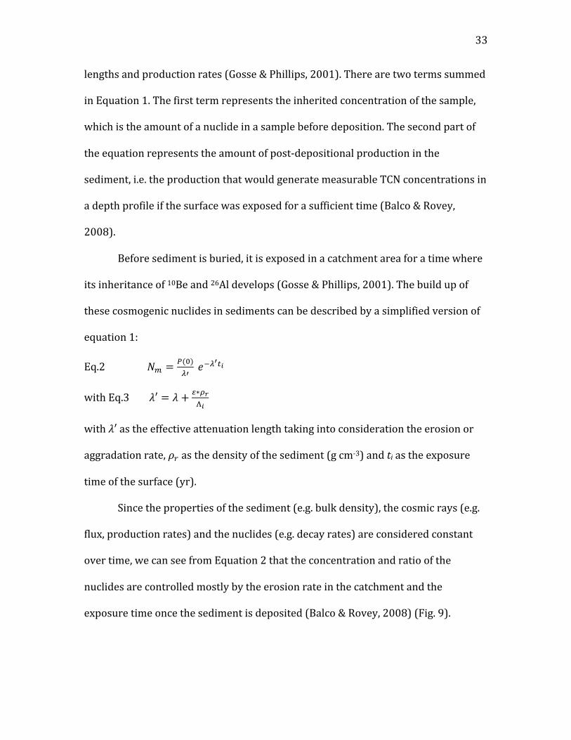
lengths and production rates (Gosse & Phillips, 2001). There are two terms summed
in Equation 1. The first term represents the inherited concentration of the sample,
which is the amount of a nuclide in a sample before deposition. The second part of
the equation represents the amount of post-‐depositional production in the
sediment, i.e. the production that would generate measurable TCN concentrations in
a depth profile if the surface was exposed for a sufficient time (Balco & Rovey,
2008).
Before sediment is buried, it is exposed in a catchment area for a time where
its inheritance of 10Be and 26Al develops (Gosse & Phillips, 2001). The build up of
these cosmogenic nuclides in sediments can be described by a simplified version of
equation 1:
Eq.2 𝑁! = !(!)!! 𝑒!!!!!
with Eq.3 𝜆′ = 𝜆 + !∗!!!!
with 𝜆′ as the effective attenuation length taking into consideration the erosion or
aggradation rate, 𝜌! as the density of the sediment (g cm-‐3) and ti as the exposure
time of the surface (yr).
Since the properties of the sediment (e.g. bulk density), the cosmic rays (e.g.
flux, production rates) and the nuclides (e.g. decay rates) are considered constant
over time, we can see from Equation 2 that the concentration and ratio of the
nuclides are controlled mostly by the erosion rate in the catchment and the
exposure time once the sediment is deposited (Balco & Rovey, 2008) (Fig. 9).

34
likewise slow erosion rates which allow a sample to reside near the surface for the fullduration of exposure and accumulate a large nuclide inventory, result in Rinit signifi-cantly below the production ratio. The value of Rinit used in determining the burial agein equation (9) has to be adjusted to account for this effect. Note that we have notconsidered soil mixing processes that increase the residence time of some quartzgrains in the soil more than expected from steady erosion alone, and further decreaseRinit. This is a secondary issue for the present purposes; for a mathematical treatmentsee Lal and Chen (2005).
We account for the dependence of Rinit on paleosol exposure time and erosionrate by another iteration scheme, as follows. First, once we have determined both an
Fig. 5. Effects of extended exposure and surface erosion on the parameter Rinit , according to equation(10). The dark lines are contours of the ratio of Rinit to the 26Al/10Be production ratio P26(0)/P10(0) as afunction of surface erosion rate and exposure time. Rinit is close to the production ratio when exposure timesare short and/or erosion is rapid, and diverges at long exposure times and low erosion rates as radioactivedecay becomes more important. The dotted gray contours show 10Be concentrations developed duringexposure, normalized to the surface production rate (this quantity has units of years, but is more sensiblythought of as the 10Be concentration in atoms g!1 given a surface 10Be production rate of 1 atom g!1 yr!1).Production due to muon interactions is not included in this plot, so it is simply a remapping of the simpleexposure island of Lal (1991). The gray regions show the range of exposure ages and erosion rates permittedfor the paleosols in this study, inferred from correcting the measured nuclide concentrations back to thetime of burial as described in the text. The boundaries of these regions reflect i) the allowable range for thesurface 10Be concentration attributable to surface exposure, and ii) 95% confidence limits on the exposuretime of the paleosols obtained from differencing the ages of the overlying till and the till in which thepaleosol is developed (for the Missouri tills—there is no constraint on the age of the till in the 3B99borehole). The important point is that even though our method provides only very weak bounds on theerosion rates and exposure times of the paleosols prior to burial, they are all in a range where the variation inRinit is small, so a large uncertainty in estimating surface production rates, exposure times, and erosion ratestranslates into only a small uncertainty in estimating Rinit and determining the burial age of the paleosol.
1097cosmogenic-nuclide dating of buried soils and sediments
Figure 9 shows that variation of the ratio of 26Al/10Be from the production
ratio (6.75) due to changes in the erosion rate and exposure time (Balco & Rovey,
2008). The graph shows that samples with high erosion rate and low exposure time
have 26Al/10Be ratios that are closer to the production ratio since they do not have
enough time to become saturated in 26Al and 10Be (Balco & Rovey, 2008).
With this in mind, let us consider the samples collected for this thesis. The
samples began as regolith along slopes in a catchment with high relief that was
prone to landslides (we can ignore the previous histories of the samples because
they are irrelevant if longer than about eight half lives of 10Be). Though there were
frequent landslides, the surface was still experiencing steady erosion over time.
This erosion kept the surface from saturating in cosmogenic nuclides, meaning that
that the ratio of 26Al/10Be should have been close to 6.75 (Balco & Rovey, 2008). The
surface processes and landslides would deliver grains of various sizes and
concentrations of 10Be and 26Al and, with the exception of rare deep-‐seated
Figure 9: Plot showing how the ratio of 26Al/10Be deviates in sediments from the production ratio (6.75) with various exposure times and erosion rates. Having high exposure time and low erosion rates results in the largest deviance due to saturation of the nuclides being reached in the soil (Balco & Rovet, 2008)
35
landslides that deliver bedrock fragments that have higher 26Al/10Be due to muonic
production (e.g. 8.2), the ratio of the average inherited 26Al/10Be in the sediment will
be 6.75, assuming no prolonged burial during storage (i.e. for more than a hundred
thousand years) (Balco & Rovey, 2008).
No definitive paleosol was recognized at the sample site, so considering the
tropical climate, the samples were most likely buried reasonably quickly (i.e. no
sample was exposed for more than about 10 ka before being buried). This means
that almost all 26Al and 10Be measured in the samples can be attributed to
inheritance. Of course this is not possible to demonstrate in the field, and will only
be known after evaluating the TCN-‐grain-‐size relationship. If the samples were
exposed for more than 10 ka, the TCN dependency with grain size would not be
visible.
Using the assumption that all of the nuclides in the sediment formed before
burial in the catchment, then their concentrations would have only decreased after
burial due to radioactive decay. It is not possible for us to know what the absolute
initial concentrations of 26Al and 10Be were in the samples unless we determine the
age, and then correct for the loss of TCN due to decay (Balco & Rovey, 2008). The
26Al/10Be in a sample will change predictably according to the different radionuclide
decay rates, and at any given time all of the samples for the different grain size
would have the same ratio, assuming they all began at 6.75 (Balco & Rovey, 2008).
36
3.4 Error mitigation and analysis
During physical processing several precautions were taken to control error.
Only one sample was ever processed at a time, and between samples all sieves,
machinery and surfaces were thoroughly cleaned. All samples were stored in clean
Ziploc bags that were labeled several times.
During chemical processing all jars that held samples were labeled several
times, and the jars were always kept covered whenever possible. The lab doors
were kept closed, and the lab has a dedicated boron-‐free HEPA-‐filtered HVAC air
purification system. Only ultrapure reagents and water were used after the initial
stages of quartz purification. All masses were determined with high-‐precision
balances. With the exception of the Teflonware and target holders, all containers
were virgin materials. The precision of the ICP-‐OES measurements for beryllium
and aluminum were typically better than 2%, so considering this and gravimetric
uncertainly of much less than 1%, the total internal random error contributed by
the chemistry is considered 2% at 1-‐sigma. AMS error is based on the Poisson
distribution-‐based precision, and is therefore dependent on the number of counts of
atoms. Error contributed by the blank subtraction is typically negligible because the
process blanks have low ratios (1.5 x 10-‐15), however if the samples were buried for
millions of years, the ratios in the samples may be comparable, and the uncertainty
in the blank subtraction can be the dominant source of measurement error.
For the calculations several assumptions were made. The assumption was
made that the erosion rate in the catchment was simple, meaning that it was

37
constant over time, with occasional landslides. The assumption was made that
during the transport of the samples from the catchment to the site of burial the
samples were not stopped at any point and exposed at surface. As well the
assumption was made that the burial of the samples was rapid and complete.
The AMS and ICP-‐MS measurements have systematic error that must be
taken into account. Error calculations are shown in Appendix 1.

38
4.0 Results
Accelerator Mass Spectrometer (AMS) analysis of the samples was conducted
at Lawrence Livermore National Lab. Two separate analyses were done, one for
26Al/27Al and one for 10Be/9Be (Appendix 1). The AMS and chemical data (e.g.
carrier and quartz masses, blank subtractions, and native aluminum and beryllium
in the quartz as measured by ICP-‐OES at DGC) were then reduced to calculate the
concentrations of 26Al and 10Be in the quartz samples, in atoms per gram. 27Al is
naturally much more abundant than 26Al, so we can assume that the aluminum
concentration measured by the ICP-‐OES represents the concentration of 27Al in the
sample. By multiplying the 27Al concentration (in atoms per gram of quartz) by the
26Al /27Al ratio measured by the AMS, the 26Al concentration for the sample can be
calculated.
For the beryllium samples, native 9Be does not occur naturally in high
enough concentrations in quartz (e.g. beryl inclusions) to help carry the 10Be
through the chemistry (0.1 µg/g or less beryllium). Therefore a beryllium carrier
(averaging 211 µg of 9Be) was added to the quartz at the beginning of chemistry.
Since the amount of carrier added was precisely measured we can calculate the
amount of 9Be in the sample. So, the 10Be concentration is determined by
multiplying the 9Be atoms from the carrier by the 10Be /9Be. The full data reduction
process is shown in a spreadsheet, in Appendix 1. The data are shown in Table 1
below.

39
Sample name 10Be Conc 10Be Unc 26Al Conc 26Al Unc 26Al/ 10Be Ratio
Ratio Unc
comb3159-‐3162 4078 312 41902 9218 10.3 2.40 TAME0.85-‐1 4676 321 31565 6944 6.8 1.56 TAME0.5-‐0.85 8137 922 27869 6131 3.4 0.84 TAME0.335-‐0.5 6654 309 31897 7017 4.8 1.07 TAME0.25-‐0.355 6437 272 36785 8093 5.7 1.28 TAME0.150-‐025 5909 311 41867 9211 7.1 1.60
The reason why the TAME 0.5-‐0.85 beryllium data is colored red is because
there was only enough BeO in the target for the AMS to do a single beryllium
measurement. After the first run, the current was too low to proceed. This means
that the data for this sample is unreliable, so it will not be used in further analysis.
Reasons for this are listed in the Discussion section.
The uncertainties for the 10Be and 26Al measurements (4-‐8% and 22% at 1-‐
sigma), which include uncertainties in the process blank subtraction and chemistry
error (2%, mostly from ICP measurement) are higher than normal (e.g. for the
measurement of the isotopes in 20 g quartz from a boulder). This is partly because
of the very low abundance of 10Be (i.e. 6000 atoms/g is much lower than the typical
105 atoms/g) but also because of challenges in chemistry when running so much
quartz with less than the normal amount of beryllium carrier (250 µg). Likewise,
the samples had high aluminum concentrations, which with such large masses of
quartz, caused changes to the elution of the aluminum and beryllium cations during
ion chromatography.
Table 1: Concentrations of 26Al and 10Be for the samples taken for this thesis are in the table above. Values are the result of the data reduction of the AMS data. All concentrations are in atoms/g

40
5.0 Discussion
5.1 Interpretations of TCN data
5.1.1 Hypothesis 1-‐ Grain-‐size dependent isochron method is viable
The concentrations of 26Al and 10Be were plotted onto an isochron plot in an
attempt to determine a burial age. The isochron plot is shown in Figure 10 below.
From the isochron plot we can see that the data defines a negative slope. This
is not an acceptable outcome on the isochron burial plot (has a positive slope) so the
data cannot be used to calculate a burial age. Thus the data suggest that the
hypothesis that an isochron chronology can be achieved using grain-‐size fractions is
false.
Figure 10: A. Isochron plot of samples from the Tauramena sample site. B. What is considered a typical isochron. The blue box represents where the data from this thesis would plot. Figure adapted from Balco & Rovey 2008.
A
B
41
The most likely reason that these data did not work out was due to very low
concentrations of the elements being present in the AMS targets. The number of
atoms stripped from the oxide target and forming a beam of 27Al or 9Be during AMS
is recorded as a current. The currents for both our aluminum and beryllium
measurements were a factor of 5X smaller than normal (Appendix 1). A low current
usually indicates that there is a problem with the chemical preparation of the target,
because there is insufficient aluminum or beryllium in the target, or there is some
other atoms in the target that are interfering with the aluminum and beryllium
atoms when they are sputtered. In this instance, it is likely that the chemistry
purified the targets sufficiently. In fact, for these targets, two additional steps were
taken to do this. First, between the anion column chemistry and cation column
chemistry, the samples were precipitated in a buffered solution to separate alkali
and alkaline earth elements from the beryllium and aluminum. Second, an
additional cation column chemistry was conducted to better separate aluminum and
beryllium from other impurities. Because of the large mass and therefore potentially
high abundances of these other unwanted cations, it is believed that a significant
mass of aluminum and beryllium were both lost during the chemistry procedures.
Additionally, because aluminum was very high, there was aluminum in the BeO
target, which may have contributed to a lower current. Furthermore, because 16%
less beryllium carrier was added to help keep the ratio of 10Be/9Be in the samples
high relative to the process blank, this contributed to a lower current.
In addition to the low current, a low abundance of the radioisotopes 10Be and
26Al was anticipated (hence the lower carrier mass added). The low abundance is

42
caused by a long burial period during which the radioisotopes decay. This lower
abundance has resulted in an insufficient number of atoms being detected to obtain
a higher precision. Precision is described by the Poisson distribution, which can be
estimated as !! where n is the number of atoms of the radionuclide measured. To
obtain a 1% precision, 10,000 counts need to be detected, whereas the 26Al samples
yielded 11 counts or less per 400 second run (three runs were attempted) and 10Be
had less than 150 counts total.
There may be other factors that influenced the poor performance of the
oxides. During the dissolution of quartz with HF, the fluorine in the acid can react
with calcium to form CaF2 crystals, which can scavenge aluminum and beryllium as
inclusions. Steps are taken to avoid these processes (e.g. the addition of a small
amount of nitric acid) but they can still occur on the small scale and result in the loss
of Al, at a rate that would be different for each sample, depending on the abundance
of unwanted cations. This is unlikely as no crystals were observed after dissolution.
Another possibility is that some of the quartz crystals dissolved had an
inclusion on beryl. This would be a large source of 9Be and would cause low
measurements of the 10Be/9Be ratio on the AMS. This does not appear to be the
case, because measurements of beryllium in quartz before dissolution did not
indicate anomalous beryllium concentrations, and because the 10Be concentrations
are similar to the concentrations achieved previously by PRIME Lab.
Therefore, while the results suggest that H1 is false, it is possible that with
samples from a region with lower erosion rates, or a different chemistry procedure
and better current but at lower precision, a positive result could be achieved.
43
5.1.2 Hypothesis 2-‐ High erosion rates in landslide prone regions will cause
imprecision
As previously stated, one of the reasons that the AMS measurements were
such low concentrations can probably be attributed to a low initial TCN
concentration in the samples, which is a result of rapid erosion rates in the
catchment area of where the samples originated. It appears that the hypothesis that
high erosion rates in the catchment area of the sediment would decrease TCN
concentrations below a point where they could not be resolved holds true.
The paleo-‐erosion rates of the catchment area can be calculated with the
collected 10Be and 26Al data individually following the method presented by Schaller
et al. (2002) and Hidy et al. (2010). Essentially this involves correcting the
measured radioisotope concentration for loss by decay during the burial time.
While the burial duration is uncertain in this case, estimates from two
measurements from Veloza et al. (unpub.) were 2.25 and 2.65 Ma. Therefore,
assuming a 2.5 Ma burial duration, the measured concentrations, corrected for
decay, are interpreted as the concentrations of the TCN in the sample at the time of
deposition. This then can be used to calculate erosion rate with the equation:
Eq.4 𝜀 = !°!!°!
where 𝜀 is the erosion rate (cm yr-‐1), 𝐶° is the TCN concentration at the time of
deposition (atoms g-‐1), Λ is the attenuation length of a cosmic ray (g cm-‐2), 𝑃° is the
production rate for a particular TCN in a catchment area (atoms g-‐1 yr-‐1) and 𝜌 is the
bulk density of the material (g cm-‐3). Full calculations are shown in Appendix 1.
44
Negev%Desert%Isreal Clapp%et%al.,%2000Costal%plne,%Texas Hidy%et%al.,%2014Arizona,%Ymua%wash Clapp,%Bierman%&%Caffee,%2002Diamond%Mountains,%CA Granger%et%al.,%2001SE,%Austrailia Heimsath%et%al.,%2000NW,%New%Mexico Clapp%et%al.,%2001Oregen%Coast%Range Heimsath%et%al.,%2001Apennines,%Italy Cyr%&%Granger,%2008SouthPCentral%Andes Atinao,%2008Wasatch%Mountains,%UT Stock%et%al.,%2009South,%Italy Cyr%et%al.,%2010Kunlun,%Tibet Dingd%et%al.,%2003High%Himalaya Vance%et%L.,%2003
The erosion rates calculated using the aluminum and beryllium data from
this thesis are shown in Figure 11 as red squares. A sampling of erosion rates from
around the world has also been included to provide comparison. It is apparent in
the diagram that there is a significant difference in the calculated erosion rates given
by the different isotopes. 10Be gave an erosion rate of 2.59±0.65 mm yr-‐1 and 26Al
Figure 11: Paleo-‐erosion rates calculated from the 26Al and 10Be data. A sample of modern catchment-‐wide erosion rates have also been plotted for comparison. The red squares are the measured erosion rates. The blue diamonds are erosion rates from literature. See Table 2 for a list of references.
Table 2: References associated with localities and erosion rates plotted in Figure 11.
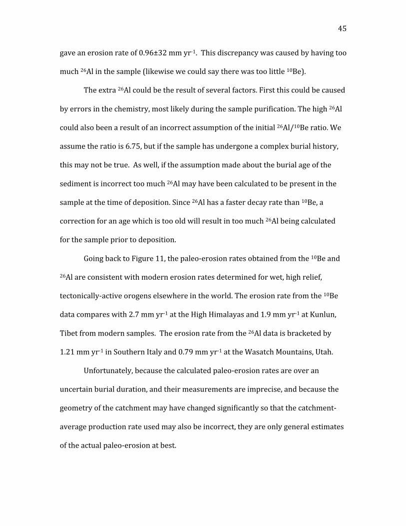
45
gave an erosion rate of 0.96±32 mm yr-‐1. This discrepancy was caused by having too
much 26Al in the sample (likewise we could say there was too little 10Be).
The extra 26Al could be the result of several factors. First this could be caused
by errors in the chemistry, most likely during the sample purification. The high 26Al
could also been a result of an incorrect assumption of the initial 26Al/10Be ratio. We
assume the ratio is 6.75, but if the sample has undergone a complex burial history,
this may not be true. As well, if the assumption made about the burial age of the
sediment is incorrect too much 26Al may have been calculated to be present in the
sample at the time of deposition. Since 26Al has a faster decay rate than 10Be, a
correction for an age which is too old will result in too much 26Al being calculated
for the sample prior to deposition.
Going back to Figure 11, the paleo-‐erosion rates obtained from the 10Be and
26Al are consistent with modern erosion rates determined for wet, high relief,
tectonically-‐active orogens elsewhere in the world. The erosion rate from the 10Be
data compares with 2.7 mm yr-‐1 at the High Himalayas and 1.9 mm yr-‐1 at Kunlun,
Tibet from modern samples. The erosion rate from the 26Al data is bracketed by
1.21 mm yr-‐1 in Southern Italy and 0.79 mm yr-‐1 at the Wasatch Mountains, Utah.
Unfortunately, because the calculated paleo-‐erosion rates are over an
uncertain burial duration, and their measurements are imprecise, and because the
geometry of the catchment may have changed significantly so that the catchment-‐
average production rate used may also be incorrect, they are only general estimates
of the actual paleo-‐erosion at best.

46
5.1.3 Was there a grain size dependence?
The measured data do not provide a 26Al vs. 10Be isochron. A probable
reason for this is related to difficulty in conducting chemistry on a large sample with
such low TCN abundance, as discussed above. However, one of the critical
assumptions of the method was that there is a grain-‐size dependency among the
TCN concentrations, owing to decreases in concentration and weathering with
depth in regolith on the catchment surface. To determine if the data reveal any
indication of this grain size dependency, the relationship between 10Be and 26Al and
grain size was investigated.
The 10Be concentrations show no variation with grain size, likely because
their low production rates did not provide sufficient scatter beyond the total
analytical uncertainty after millions of years of decay (Fig. 12).
As well, due to the low measured values and the large errors, none of the values can
be statistically distinguished from on another. This being the case, these values give
nowhere near enough spread to define a line on an isochron plot.
Figure 12: Calculated 10Be concentrations for samples of different grain sizes.
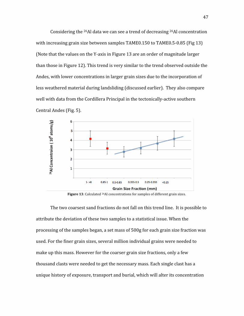
47
Considering the 26Al data we can see a trend of decreasing 26Al concentration
with increasing grain size between samples TAME0.150 to TAME0.5-‐0.85 (Fig 13)
(Note that the values on the Y-‐axis in Figure 13 are an order of magnitude larger
than those in Figure 12). This trend is very similar to the trend observed outside the
Andes, with lower concentrations in larger grain sizes due to the incorporation of
less weathered material during landsliding (discussed earlier). They also compare
well with data from the Cordillera Principal in the tectonically-‐active southern
Central Andes (Fig. 5).
The two coarsest sand fractions do not fall on this trend line. It is possible to
attribute the deviation of these two samples to a statistical issue. When the
processing of the samples began, a set mass of 500g for each grain size fraction was
used. For the finer grain sizes, several million individual grains were needed to
make up this mass. However for the coarser grain size fractions, only a few
thousand clasts were needed to get the necessary mass. Each single clast has a
unique history of exposure, transport and burial, which will alter its concentration
Figure 13: Calculated 26Al concentrations for samples of different grain sizes.
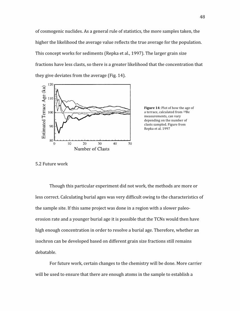
48
of cosmogenic nuclides. As a general rule of statistics, the more samples taken, the
higher the likelihood the average value reflects the true average for the population.
This concept works for sediments (Repka et al., 1997). The larger grain size
fractions have less clasts, so there is a greater likelihood that the concentration that
they give deviates from the average (Fig. 14).
5.2 Future work
Though this particular experiment did not work, the methods are more or
less correct. Calculating burial ages was very difficult owing to the characteristics of
the sample site. If this same project was done in a region with a slower paleo-‐
erosion rate and a younger burial age it is possible that the TCNs would then have
high enough concentration in order to resolve a burial age. Therefore, whether an
isochron can be developed based on different grain size fractions still remains
debatable.
For future work, certain changes to the chemistry will be done. More carrier
will be used to ensure that there are enough atoms in the sample to establish a
Figure 14: Plot of how the age of a terrace, calculated from 10Be measurements, can vary depending on the number of clasts sampled. Figure from Repka et al. 1997
49
strong current during AMS measurements. Less quartz will be dissolved for each
sample to decrease the amount of unwanted cations entering the columns.
For field techniques, larger grain size fractions should be targeted during
sampling to insure enough mass for these grain size fractions is collected. This
experiment relied on sand fractions to test if the subtle dependence on grain size
was enough to provide the scatter needed to define an isochron. Experiments
relying on scatter during the development of depth profiles after deposition prior to
burial, or on the possibility that five or more individual cobbles may have sufficient
scatter to define an isochron have already been conducted.
This thesis is the second attempt to calculate a burial age for one particular
sediment deposit in the Colombian Andes. I believe that it should not be the last.
Despite the sample site having a high paleo-‐erosion rate and an old burial age, it is
still a good location for attempting burial dating. It is a very good location to attempt
to push the limits of TCN burial dating, and could potentially provide important
information about the impact of climatic change on landscape evolution in the
Colombian Andes.
As for the grain-‐size dependent isochron method, I believe that it should be
attempted again. The results from this thesis pertaining to the effectiveness of this
method are inconclusive. However the amount of evidence showing TCN
concentration dependence with grain size in regions of high relief, paired with how
useful this method could be in areas where there are no paleosols and no cobbles
warrants further testing of the grain-‐size dependent isochron method.
50
6.0 Conclusion
In conclusion, the effectiveness of a grain-‐size dependent isochron method has
proven inconclusive. The collected samples gave measured concentrations for 26Al
that ranged from 2.79 to 4.19 X 10⁴ atoms/g (±21% 1-‐sigma) and for 10Be from 4.08
to 8.14 X 10³ (±4-‐8% 1-‐sigma). These measured values were too low and had too
little resolution to be able to define an isochron, meaning that effectiveness of the
grain-‐size dependent isochron method could not be tested.
The reason for these low measured values can most likely be attributed to
high erosion rates in the catchment area, resulting in low initial concentrations of
TCN in the samples. 26Al and 10Be may have also been lost during certain steps of
the chemical processing since extra quartz mass was dissolved and extra
purification steps were needed.
With the collected data, paleo-‐erosion rates were calculated for the
catchment, with 10Be giving an erosion rate of 2.59 mm yr-‐1 (±25% 1-‐sigma) and 26Al
0.97 mm yr-‐1 (±33% 1-‐sigma). These rates suggest that the catchment area was
undergoing rapid erosion, at a rate equivalent to other tectonically active orogens.

51
7.0 Reference list
Antinao J. L. (2008). Quaternary Landscape Evolution of the Southern Central Andes of Chile Quantified Using Landslide Inventories, 10Be and 36Cl Cosmogenic Isotopes and (U-‐Th)/He Thermochronology (Doctorial thesis). Retrieved from Dalhousie University. Balco, G., & Rovey, C. (2008). An isochron method for cosmogenic-‐nuclide dating of buried soils and sediments. American Journal of Science, 308 (10), 1083-‐ 1114. Balco, G., Rovey, C. (2010). Absolute chronology for major Pleistocene advances of the Laurentide Ice Sheet. Geology, 38(9), 795-‐798. Balco, G., Soreghan, G. S., Sweet, D. E., Marra, K. R., & Bierman, P. R. (2013). Cosmogenic-‐nuclide burial ages for Pleistocene sedimentary fill in Unaweep Canyon, Colorado, USA. Quaternary Geochronology, 18, 149-‐157. Belmont, P., Pazzaglia, F.J., & Gosse, J. (2007). Cosmogenic 10Be as a tracer for hillslope and channel sediment dynamics in the Clearwater River, western Washington State. Earth and Planetary Science Letters, 264 (1-‐2), 123-‐135. Cortes M., Angelier, J., Colletta, B. (2006). Structure and tectonics of the central segment of the Eastern Cordillera of Colombia. Journal of South American Earth Sciences, 21 (4), 437-‐465. Clapp, E. M., Bierman, P. R., & Caffee, M. (2002). Using 10 Be and 26 Al to determine sediment generation rates and identify sediment source areas in an arid region drainage basin. Geomorphology, 45(1), 89-‐104. Clapp, E. M., Bierman, P. R., Nichols, K. K., Pavich, M., & Caffee, M. (2001). Rates of sediment supply to arroyos from upland erosion determined using in situ produced cosmogenic 10 Be and 26 Al. Quaternary Research, 55(2), 235-‐245. Clapp, E. M., Bierman, P. R., Schick, A. P., Lekach, J., Enzel, Y., & Caffee, M. (2000). Sediment yield exceeds sediment production in arid region drainage basins. Geology, 28(11), 995-‐998. Cyr, A. J., & Granger, D. E. (2008). Dynamic equilibrium among erosion, river incision, and coastal uplift in the northern and central Apennines, Italy. Geology, 36(2), 103-‐106.
52
Cyr, A. J., Granger, D. E., Olivetti, V., & Molin, P. (2010). Quantifying rock uplift rates using channel steepness and cosmogenic nuclide–determined erosion rates: Examples from northern and southern Italy. Lithosphere, 2(3), 188-‐198. Dingd, L., Liud, T., Donga, W., Caffeee, M. W., & Jullf, A. J. T. (2003). Erosion history of the Tibetan Plateau since the last interglacial: constraints from the first studies of cosmogenic 10Be from Tibetan bedrock. Earth and Planetary Science Letters, 217(33), 33-‐42. Gibbard, P. L., Head, M. J., & Walker, M. J. (2010). Formal ratification of the Quaternary System/Period and the Pleistocene Series/Epoch with a base at 2.58 Ma. Journal of Quaternary Science, 25(2), 96-‐102. Gosse, J., & Phillips F. M. (2001). Terrestrial in situ cosmogenic nuclides: theory and application. Quaternary Science Reviews, 20, 1474-‐1560. Granger, D.E., & Muzikarb, P. F. (2001). Dating sediment burial with in situ-‐produced cosmogenic nuclides: theory, techniques, and limitations. Earth and Planetary Science Letters, 188, 269-‐281. Granger, D. E., Riebe, C. S., Kirchner, J. W., & Finkel, R. C. (2001). Modulation of erosion on steep granitic slopes by boulder armoring, as revealed by cosmogenic 26 Al and 10 Be. Earth and Planetary Science Letters, 186(2), 269-‐281. Gregory-‐Wodzicki K.M. (2000) Uplift History of the Northern and Central Andes: a review. GSA Bulletin, 112 (7), 1091–1105. Heimsath, A. M., Dietrich, W. E., Nishiizumi, K., & Finkel, R. C. (2001). Stochastic processes of soil production and transport: Erosion rates, topographic variation and cosmogenic nuclides in the Oregon Coast Range. Earth Surface Processes and Landforms, 26(5), 531-‐552. Heimsath, A. M., Chappell, J., Dietrich, W. E., Nishiizumi, K., & Finkel, R. C. (2000). Soil production on a retreating escarpment in southeastern Australia. Geology, 28(9), 787-‐790. Hidy, H. J. (2013). Cosmogenic Nuclide Quantification of Paleo-‐Fluvial Sedimentation Rates in Response to Climate Change (Doctorial dissertation). Retrieved from Dalhousie University. Hidy, A. J., Gosse, J. C., Blum, M. D., & Gibling, M. R. (2014). Glacial–interglacial variation in denudation rates from interior Texas, USA, established with cosmogenic nuclides. Earth and Planetary Science Letters, 390, 209-‐221.

53
Hidy, A. J., Gosse, J. C., Pederson, J. L., Mattern, J. P., & Finkel, R. C. (2010). A geologically constrained Monte Carlo approach to modeling exposure ages from profiles of cosmogenic nuclides: An example from Lees Ferry, Arizona. Geochemistry, Geophysics, Geosystems, 11(9).
Chicago Kohl, C. P., & Nishiizumi, K. (1992). Chemical isolation of quartz for measurement of in-‐situ -‐produced cosmogenic nuclides. Geochimica et Comochimica Acta. 56, 3583-‐3587. Lal, D. (1991). Cosmic ray labeling of erosion surfaces: in situ nuclide production rates and erosion models. Earth and Planetary Science Letters, 104(2), 424-‐ 439. Parra M., Mora, A., Jaramillo, C., Torres, V., Zeilinger G., & Strecker M. R. (2010) Tectonic controls on Cenozoic foreland basin development in the north-‐ eastern Andes, Colombia. Basin Research, 22, 874–903. Puchol N., LavlZ' , J., Lupker, M., Blard, P-‐H., Gallo, F., France Lanord, C., & ASTER Team. (2014). Grain-‐size dependent concentration of cosmogenic 10Be and erosion dynamics in a landslide-‐dominated Himalayan watershed. Geomorpholgy, 224, 55-‐68. Rees-‐Jones, J. (1995). Optical dating of young sediments using fine-‐grain quartz.
Ancient TL, 13(2), 9-‐14. Repka J. L., Anderson R. S., & Finkel R. C. (1997). Cosmogenic dating of fluvial terraces, Fremont River, Utah. Earth and Planetary Science Letters. 152, 59-‐ 73. Rybczynski, N., Gosse, J. C., Harington, C. R., Wogelius, R. A., Hidy, A. J., & Buckley, M. (2013). Mid-‐Pliocene warm-‐period deposits in the High Arctic yield insight into camel evolution. Nature communications, 4, 1550. Schaller, M., Von Blanckenburg, F., Veldkamp, A., Tebbens, L. A., Hovius, N., & Kubik, P. W. (2002). A 30 000 yr record of erosion rates from cosmogenic 10 Be in Middle European river terraces. Earth and Planetary Science Letters, 204(1), 307-‐320. Stock, G. M., Frankel, K. L., Ehlers, T. A., Schaller, M., Briggs, S. M., & Finkel, R. C. (2009). Spatial and temporal variations in denudation of the Wasatch Mountains, Utah, USA. Lithosphere, 1(1), 34-‐40.

54
Vance, D., Bickle, M., Ivy-‐Ochs, S., & Kubik, P. W. (2003). Erosion and exhumation in the Himalaya from cosmogenic isotope inventories of river sediments. Earth and Planetary Science Letters, 206(3), 273-‐288. Veloza, G., Taylor, M., Mora, A., & Gosse, J. (Unpub). Active mountain building along the eastern Colombian Sub-‐Andes: A folding history from deformed terraces across the Tame Anticline, Llanos Basin. University of Kansas, Lawrence KS. Veloza Fajardo, G. E. (2012). Active faulting and Quaternary slip rates of the Colombian sub-‐Andes (Doctoral dissertation, University of Kansas).


