

Finance and Economics Discussion Series Divisions of Research & Statistics and Monetary Affairs
Federal Reserve Board, Washington, D.C.
The Effect of Housing Government-Sponsored Enterprises on Mortgage Rates
Wayne Passmore, Shane M. Sherlund, and Gillian Burgess 2005-06
NOTE: Staff working papers in the Finance and Economics Discussion Series (FEDS) are preliminary materials circulated to stimulate discussion and critical comment. The analysis and conclusions set forth are those of the authors and do not indicate concurrence by other members of the research staff or the Board of Governors. References in publications to the Finance and Economics Discussion Series (other than acknowledgement) should be cleared with the author(s) to protect the tentative character of these papers.
The Effect of Housing Government-Sponsored
Enterprises on Mortgage Rates
Wayne Passmore, Shane M. Sherlund, and Gillian Burgess
Federal Reserve Board1
Forthcoming in Real Estate Economics2
Please do not cite or circulate without permission of the authors.
ABSTRACT
We derive a theoretical model of how jumbo and conforming mortgage rates are determined and how the jumbo-conforming spread might arise. We show that mortgage rates reflect the cost of funding mortgages and that this cost of funding can drive a wedge between jumbo and conforming rates (the jumbo-conforming spread). Further, we show how the jumbo-conforming spread widens when mortgage demand is high or core deposits are not sufficient to fund mortgage demand, and tighten as the mortgage market becomes more liquid and realizes economies of scale. Using MIRS data for April 1997 through May 2003, we estimate that the GSE funding advantage accounts for about seven basis points of the 15-18 basis point jumbo-conforming spread.
1 The opinions, analysis, and conclusions of this paper are solely the authors’ and do not necessarily reflect those of the Board of Governors of the Federal Reserve System. Ms. Burgess is now a student at New York University’s School of Law. We wish to thank Mary DiCarlantonio, Paul Landefeld, and Cathy Gessert for their excellent research assistance. We also wish to thank three anonymous referees and our many colleagues at the Federal Reserve Board and at the Federal Reserve Banks for their useful and constructive comments, including Glenn Canner, William Cleveland, Darrel Cohen, Chris Downing, Karen Dynan, Ed Ettin, Kieran Fallon, Ron Feldman, Scott Frame, Steve Friedman, Mike Gibson, Alan Greenspan, Diana Hancock, Richard Insalaco, Kathleen Johnson, Myron Kwast, Andreas Lehnert, Brian Madigan, Norman Morin, Steve Oliner, Pat Parkinson, Richard Peach, Karen Pence, Bob Pribble, Brian Sack, David Stockton, Pat White, and David Wilcox. We would also like to thank the staffs at the Congressional Budget Office, the Council of Economic Advisors, the Department of the Treasury, and the Office of Management and Budget for their comments, including David Torregrosa and Mario Ugoletti. We also thank William Greene for helpful comments. 2 Real Estate Economics is the Journal of the American Real Estate and Urban Economics Association and is located at the Leeds School of Business, University of Colorado-Boulder, Boulder, CO, 80309-0419 (e-mail: [email protected]). Portions of this paper were included in an earlier version of “The GSE Implicit Subsidy and the Value of Government Ambiguity,” Federal Reserve Finance and Economics Discussion Series, No. 2003-64, December 2003.
- 2 -
1. Introduction
Congress created two government-sponsored enterprises, the Federal National
Mortgage Association (Fannie Mae) and the Federal Home Loan Mortgage Corporation
(Freddie Mac) with the goal of providing banks, thrifts, and other mortgage originators
with a liquid secondary market that would provide an alternative to funding mortgages
with deposits. A secondary mortgage market allows mortgage originators to respond
more quickly to fluctuating mortgage demand and to lower mortgage rates for some
homeowners when mortgage demand is high.
When Congress created the GSE charters, they provided the GSEs with a variety
of special benefits.3 Initially, many viewed these benefits as a way to enhance the GSEs’
efforts in establishing a secondary mortgage market. However, with the secondary
mortgage market well established and with many other well-functioning purely private
secondary markets, the justification for the GSEs’ benefits has shifted to the GSEs’
success in lowering mortgage rates and in encouraging affordable housing.
The GSEs benefit from the government-sponsored status because purchasers of
their debt assume that the government will not allow the GSEs to fail, even though the
government has made no explicit promise to bail out the GSEs should problems arise.
This ambiguous government relationship creates an implicit government subsidy to the
GSEs that is worth billions of dollars (CBO, 2001). In this paper, we estimate the
proportion of this implicit subsidy that GSEs transmit to homeowners via lower mortgage
rates.
Like many previous studies, this paper focuses on the difference in mortgage rates
observed on mortgages that exceed the size limit imposed on GSE mortgage purchases
(jumbo mortgages) and mortgages below this size limit. Many previous studies assume
that the spread between jumbo and conforming mortgage rates is a measure of the effect
of GSEs. This assumption ignores segmentation of the jumbo securitization market as
well as the effects of bank funding capacity, banks’ investment alternatives, and
fluctuating mortgage demand on mortgage rates. When one considers a hypothetical
world without GSEs, researchers need to consider both the possibility that conforming
rates will rise and that jumbo rates will fall. Currently, the jumbo mortgage securitization
3 A review of these benefits can be found in Mankiw (2003) and CBO (2001).
- 3 -
market is artificially segmented from the conforming market because of the conforming
loan limit and therefore cannot realize the economies of scale or scope of the conforming
MBS market.4 Thus, the jumbo-conforming spread is an upper bound on the extent to
which mortgage rates might rise if GSEs lost their special status. Our research suggests
that the typical jumbo-conforming spread is between 15 and 18 basis points and that the
GSE funding advantage likely accounts for about seven basis points of this difference.
2. The Effect of the GSE Implicit Subsidy on Mortgage Rates
Given the many intermediaries between the source of the subsidy (investors who
view the GSEs as backed by the government) and the target of the subsidy
(homeowners), the GSEs’ presence does not necessarily change mortgage rates very
much. As argued by Goodman and Passmore (1992) and Hermalin and Jaffee (1996),
much of the subsidy may not be transmitted to homeowners. This is because the
conforming mortgage market has many of the conditions required for imperfect
competition among competitors – two competitors (Fannie Mae and Freddie Mac) with
roughly equal market share, homogeneity of product, high entry and exit barriers, and
each with almost infinite production capacity.5 In addition, Fannie and Freddie – like all
insurers of credit risk – face an adverse selection problem, which requires that they
include a “lemons premium” in the purchase price they offer for mortgages.
Theoretically, the GSEs’ efforts to avoid adverse selection could then completely absorb
the subsidy (Passmore and Sparks, 1996). This outcome has become more likely with the
advent of automated underwriting because mortgage originators can determine, with little
cost, whether GSEs will purchase a mortgage (Passmore and Sparks, 2000). Finally,
because the mortgage originators who are depository institutions always decide first
which mortgages to keep and which to sell (a “first mover advantage”), the GSEs – even
if they desire to pass on a subsidy to homeowners – might not be able to use the mortgage
banking system to actually transmit the subsidy because of the banks’ relative advantage
4 Passmore, Sparks, and Ingpen (2002) investigate the effect of this segmentation. Other factors can also create differences between conforming and jumbo mortgage rates – differences that are unrelated to the GSEs. For example, Ambrose, Buttimer, and Thibodeau (2001) find that the variance in house prices is U-shaped, possibly because of risk-based pricing, and therefore contributes to the jumbo-conforming spread. 5 Neither study, however, is able to establish that Fannie and Freddie actually collude.

- 4 -
in bargaining over pricing and underwriting standards (Heuson, Passmore, and Sparks,
2001).
Congress created the GSEs with the goal of providing banks with a source of
mortgage funding other than deposits. The GSEs enable banks to sell mortgages into a
secondary market during times when high mortgage demand and limits on bank capacity
for holding additional assets constrain mortgage funding. Putting aside the more
complicated arguments about the relative bargaining power of GSEs outlined above, a
secondary mortgage market – whether GSEs are involved or not – enables mortgage
originators to respond more quickly to fluctuating mortgage demand and lowers
mortgage rates for some homeowners when mortgage demand is high.6 GSEs may or
may not provide this “extra capacity” to the banking system at a lower cost than private
securitizers.
Mortgage rate studies based on data from the late 1980s and early 1990s generally
conclude that mortgage rates for conforming mortgages were about 20 to 40 basis points
less than mortgage rates for jumbo mortgages (Hendershott and Shilling, 1989;
Cotterman and Pearce, 1996). Passmore, Sparks, and Ingpen (2002) show that better
screening of the data combined with the use of more up-to-date information lowers the
estimate of the typical spread between jumbo and conforming mortgage rates to about 20
basis points. McKenzie (2002) provides an extensive survey of this literature and
estimates the spread to be 22 basis points over a long horizon (1986-2000) and 19 basis
points during a more recent period (1996-2000). Torregrosa (2001) found similar results
for this latter period (1995-2000), with estimates ranging from 18 to 25 basis points
depending upon the estimation technique and screening of the data.7
Ambrose, LaCour-Little, and Sanders (2002) conduct a unique study that, unlike
many other studies of the effect of GSEs on mortgage rates, does not rely on the Federal
Housing Finance Board’s Mortgage Interest Rate Survey (MIRS). Using data from an
6 Ambrose and Thibodeau (2004) find that the GSEs’ affordable housing goals increased the supply of mortgage credit to underserved markets, particularly during the refinance wave of 1998. 7 The GSEs also produce studies arguing that they lower mortgage rate volatility as well as lower mortgage rates (Naranjo and Toevs, 2002). However, simultaneous movements of mortgage rates, mortgage spreads, volatility, and GSE purchase activity likely confound these volatility impact estimates. As a result, the estimates likely reflect simultaneity bias. Unfortunately, there has been little independent research in this area. In addition, these studies rarely address how a GSE behaves differently than other non-GSE private purchasers in secondary markets and thus why government sponsorship is needed.

- 5 -
unidentified large national lender, they have much better measures of borrower credit
quality and of a mortgage’s conforming loan status than studies based on the MIRS data.
After taking into account borrower characteristics, house price volatility, and endogeneity
and sample selection issues, they find that jumbo mortgage rates are about 27 basis points
higher than conforming mortgages. Further, they decompose this spread into the
conforming-nonconforming8 spread (9 basis points), the jumbo-nonconforming spread
(15 basis points), and house price volatility (3 basis points). They conclude that the
GSEs account for between 9 and 24 basis points of the jumbo-conforming spread,
depending on whether one perceives the jumbo-conforming spread or the conforming-
nonconforming spread as being a result of GSE activities.
3. GSEs, the Banking Industry, and the Jumbo-Conforming Spread
The Demand for Mortgages
Using a simple model of mortgage demand, we illustrate that the jumbo-
conforming spread changes with fluctuations in mortgage demand, the attractiveness of
banks’ alternative non-mortgage investments, and with the banking industry’s capacity to
collect core deposits. We assume that households maximize the utility they receive from
their allocation of wealth. We use a quadratic utility function, so that household utility
increases as housing wealth increases until wealth reaches the bliss point, W*. Any
increase in housing wealth beyond W* decreases household utility. Given a certain value
of housing wealth, w, household utility is then
( )2*1( ) .
2U w w W= − − (3.1)
At the time a mortgage payment is due, the household must decide whether to pay
or to default on the mortgage. In our one-period model, we assume that the household
makes a down payment, p, which is a constant percentage of the total mortgage amount,
M. Then the household must repay the entire mortgage balance with interest, (1 + rM)M,
or default on the mortgage. The house is then sold at its realized liquidation value.
8 A nonconforming loan satisfies the GSEs’ loan size requirement, but fails to meet some other criteria (for example, LTV ratio and credit score requirements).

- 6 -
The liquidation value of the house (as a percentage of the purchase price), l, has a
distribution that is known ex ante to both the borrower and the bank extending the
mortgage. The household decides whether to repay the mortgage or default after
observing the realized liquidation value. If the amount of the mortgage plus interest,
(1 + rM)M, less the default cost, cdef M, is greater than the liquidation value of the house,
lM, the household defaults. Otherwise, the household repays. The default cost
encompasses the stigma that the household incurs from defaulting on such a large debt.
This stigma mainly takes the form of a lower credit rating.
Given the distribution of house liquidation values, f(l), repayments and defaults
have known probabilities. The household repays with probability q and therefore
defaults with probability (1 – q), where
.)(1
∞
−+
=defM cr
dllfq (3.2)
Housing wealth depends on whether the household repays the mortgage. If the
household does repay, housing wealth is the difference between the realized liquidation
value and the total amount paid on the house:
,)1(1
Mrp
prplw M
tR +−−−−= (3.3)
where rt is the risk-free Treasury rate. Here, the first expression is the gross proceed
from selling the house less the down payment and the opportunity cost of the down
payment. Housing wealth under default is the amount lost from the down payment plus
the cost of default:
.1
Mcp
prpw def
tD −−−−= (3.4)
Expected household utility is therefore
[ ] ( ) ( )( ) (1 ) .R DE U w qU w q U w= + − (3.5)
The household maximizes expected utility with respect to mortgage size, resulting in the
first-order condition:

- 7 -
[ ] [ ] [ ]
.01
*1
)1(
)1(1
*)1(1
)(
=−−−−−−
−−−−+
+−−
−−−+−−
−−=
deft
deft
Mt
Mt
cp
prpWMc
p
prpq
rp
prplEWMr
p
prplEq
dM
wUdE
(3.6)
This implies that the household’s optimal mortgage size is
[ ]
[ ].*
1)1()1(
1
1)1()1(
1*
22W
cp
prpqr
p
prplEq
cp
prpqr
p
prplEq
M
deft
Mt
deft
Mt
−−−−−++−
−−−
−−−−−++−
−−−
= (3.7)
Under this formulation, mortgage demand depends on optimal housing wealth (W*), the
risk-free interest rate (rt), the down payment ratio (p), the cost of default (cdef), expected
house prices (E[l]), the probability of default (q), and the mortgage rate (rM).
The Bank Cost Function and the Supply of Mortgages
Turning now to the supply side of the market, we differentiate between two types
of financial institutions that issue mortgages: Commercial banks and mortgage bankers.
Commercial banks typically fund mortgages using deposits (and are therefore required to
build the “bricks and mortar” associated with raising core deposits). Primary mortgage
originators, however, sell their mortgages shortly after origination. Both entities can sell
mortgages they originate in the secondary mortgage market, but each entity has very
different cost structures, affecting the mortgage supply function.
To collect a given amount of deposits, banks must raise capital, K, to invest in
bricks and mortar. Banks pay the market rate on equity, re, for this capital. Deposits cost
banks cdep < re. Bricks and mortar place a capacity constraint, D , on the amount of
deposits, D, and therefore the amount of mortgages that banks can hold. If mortgage
demand exceeds this capacity constraint, banks must sell the excess mortgages.
Banking profits will depend on whether or not deposit capacity is adequate. In
the low demand case, banks can retain all the mortgages they originate. They invest their
excess deposits in an alternative investment that produces a lower rate of return than
mortgages, ralt. The return on mortgages depends on whether households repay or
default. In repayment, banks receive the value of the mortgage plus interest. However,
- 8 -
in default, banks receive the liquidated value of the house. The expected return on
mortgages is then
[ ](1 ) (1 ) .m Mr q r M q E l= + + − (3.8)
The expected profits in the low demand case are
2( ) ,2
L
oL m L alt L L e dep
cr M r D M M r K c Dπ = + − − − − (3.9)
where ML < D ≤ D and coL is the cost of origination.9
Banks maximize expected profits with respect to the dollar volume of mortgages
made. In the low demand case, this leads to the first-order condition:
.0=−−= L
L
oaltm
L
L McrrdM
dπ (3.10)
The marginal cost function for banks in the low demand case is thus
.*
L
L
oalt
L
m Mcrr += (3.11)
In the high demand case, banks must sell the amount of mortgages in excess of
the deposit capacity. As a result, they face higher origination costs, coH, because of
overtime or using less-skilled workers. Expected profits in the high demand case are
2 2( )( ) ( )2 2
L HJ o oH m m alt p H H e dep
c cr D r r c M D D M D r K c Dπ = + − − − − − − − −
(3.12)
for jumbo loans and
2 2( )( ) ( )2 2
L HC o oH m m alt gse H H e dep
c cr D r r c M D D M D r K c Dπ = + − − − − − − − −
(3.13)
for conforming loans, where MH > D ≥ D and cp > cgse represent the securitization fees
for purely private securitizers and GSEs, respectively.
Banks again maximize expected profits with respect to the total volume of
mortgages made, resulting in the first-order conditions:
( ) 0J
HHm alt p o H
H
dr r c c M D
dM
π = − − − − = (3.14)
9 We have assumed that origination costs are quadratic in the amount of mortgages extended.

- 9 -
and
( ) 0.C
HHm alt gse o H
H
dr r c c M D
dM
π = − − − − = (3.15)
The marginal cost functions for the high demand case are thus
, * ( )H J H
m alt p o Hr r c c M D= + + − (3.16)
for jumbo loans and
, * ( )H C H
m alt gse o Hr r c c M D= + + − (3.17)
for conforming loans.
In the short run, the deposit capacity of banks is fixed at a multiple of the amount
of capital raised,
.D Kδ= (3.18)
In the long run, however, banks can raise more capital to increase this capacity. Banks
adjust the deposit capacity so that the marginal cost of increasing capacity equals the
marginal cost of securitization at the point where M = D (equate 3.10 and 3.15, then
solve for M = D ). The optimal capacity is then
.gse
L
o
cD
c= (3.19)
The Mortgage Banker Cost Function and the Supply of Mortgages
Mortgage bankers obtain private sources of short-term funding, paying a rate of
return repo, to finance mortgages for the short period of time between origination and
securitization. Mortgage bankers require only a small amount of capital, KMB, for which
they must pay an equity rate, reMB. For mortgages that they originate, mortgage bankers
incur a cost of origination, coMB.
Mortgage banking expected profits are
MBMB
MB
oMB
MB
eMBpm
J
MB MrepoMc
KrMcr ⋅−−−−= 2
2)(π (3.20)
for jumbo loans and
MBMB
MB
oMB
MB
eMBgsem
C
MB MgseMc
KrMcr ⋅−−−−= 2
2)(π (3.21)
- 10 -
for conforming loans. The first-order conditions are:
0=−−−= repoMccrdM
dMB
MB
opm
MB
J
MBπ (3.22)
and
.0=−−−= gseMccrdM
dMB
MB
ogsem
MB
C
MBπ (3.23)
The marginal cost functions are then
repoMccr MB
MB
op
JMB
m ++=*, (3.24)
for jumbo loans and
.*, gseMccr MB
MB
ogse
CMB
m ++= (3.25)
for conforming loans.
Exhibit 1 depicts these cost functions (equations 3.11, 3.16, 3.17, 3.24, and 3.25).
The upper panel shows how mortgage rates will vary in the jumbo and conforming
markets as a function of the level of mortgages. The upper-left quadrant is the jumbo
market; the lower-right quadrant is the conforming market; and the upper-right quadrant
and the lower panel (a blown-up version of the upper-right quadrant) map conforming
mortgage rates to jumbo mortgage rates as an implicit function of the level of mortgages.
The vertical deviation from the 45o line in these latter plots represents the jumbo-
conforming spread. In each graph, the dashed-dotted lines represent the under-capacity
portion of commercial banks’ supply curve while the dotted lines show the over-capacity
portion. The dashed lines depict the mortgage banker’s supply curve. Consumers, of
course, will choose the lower cost of these two alternatives (commercial banks versus
mortgage bankers); hence, we denote the industry supply curve in bold. Consumers may
also have, on aggregate, varying degrees of housing demand. Thus, we depict three
levels for mortgage demand – low, middle, and high – which, in our model, could result
from low, medium, and high levels of W*, respectively. These demand curves are the
dashed-gray lines in the exhibit.
As shown in the exhibit, jumbo and conforming mortgage rates are identical when
housing demand is low (the equilibrium depicted by box A in the upper panel). This is
because banks have sufficient resources to fund the aggregate level of mortgages,

- 11 -
therefore bypassing the need to securitize mortgages in the secondary market. 10 In this
case, all mortgages – jumbo and conforming – have the same rate and there is no jumbo-
conforming spread. However, once commercial banks surpass their capacity, the
secondary market plays a vital role in the determination of jumbo and conforming rates.
In the conforming market, banks can sell excess mortgages to the GSEs. However, in the
jumbo market, banks must sell to private conduits that have higher costs than the GSEs.
This results in the jumbo-conforming spread because GSE securitization is less costly to
banks (the box B equilibrium). Lastly, when demand is high (box C’s equilibrium),
mortgage bankers deliver the lowest cost mortgages to consumers. Once again,
conforming loans may be sold to the lower-cost GSEs, but jumbo loans must be sold to
purely private securitizers. This leads to a widening jumbo-conforming spread.
4. Measuring How GSEs Affect Mortgage Rates
Like Ambrose et al. (2002), we believe that other factors besides the GSEs
influence the difference between jumbo and conforming mortgage rates. Our model
highlights that the jumbo-conforming spread will vary across regions and across time for
reasons unrelated to the GSEs’ activities. As a result, the jumbo-conforming spread is a
poor measure of the GSEs’ influence on mortgage rates. As illustrated in the theoretical
model above, the jumbo-conforming spread fluctuates with mortgage demand (it widens
when demand is high), with banks’ funding capacity (it widens when core deposits are
scarce), and with the state of jumbo market securitization (it narrows as this market
becomes more liquid and realizes economies of scale). Thus, the GSEs’ implicit subsidy
is only one element of the jumbo-conforming spread.
To see this more clearly, consider the pricing of mortgages from our theoretical
framework. In the conforming market, mortgage rates are set according to
.&32 DemandSupplyFactorsRiskCostFundingGSEr C
M γγ ++= (4.1)
GSE profit maximization suggests that GSE Funding Cost is cgse + (1 – w)(cp – cgse),
where w is the pass-through rate and (1 – w)(cp – cgse) is the markup over cgse. The GSEs
10 Interestingly, we find evidence that the proportion of newly-originated conventional conforming mortgages sold to the GSEs increases with mortgage demand and thus depository institutions tend to keep a larger proportion of mortgages when demand is low.

- 12 -
set w in response to potential competition from non-GSE funders of mortgages. A pass-
through rate close to zero indicates that mortgage rates are set from cgse, whereas pass-
through rate close to one suggests that mortgage rates are set from cp. Thus,
.&)1( 32 DemandSupplyFactorsRiskcwwcr pgse
C
M γγ ++−+= (4.2)
Notice that the pass-through rate is the coefficient on cgse, not cp. In the jumbo market,
mortgage rates are set so that
.&32 DemandSupplyFactorsRiskCostFundingNonGSEr J
M φφ ++= (4.3)
Here, NonGSE Funding Cost is equal to cp so that
.&32 DemandSupplyFactorsRiskcr p
J
M φφ ++= (4.4)
In these equations, mortgage rates depend on the source of funding, risk factors, supply
and demand factors, and, in the conforming market, the pass-through rate. Note that we
allow the pricing of risk, supply, and demand factors to differ across market segments.
We can now write the jumbo-conforming spread as
( ) .&32 DemandSupplyFactorsRiskccwrr gsep
C
M
J
M ββ ++−=− (4.5)
This last equation relates the jumbo-conforming spread to differences in funding costs
(through the pass-through), risk factors, and supply and demand factors across the jumbo
and conforming markets.
We therefore modify the traditional regression approach to control for these
factors in estimating the difference between conforming and jumbo mortgage rates. Our
approach for estimating the effect of the GSEs on mortgage rates involves two sequential
regressions.11 The first step captures, in a very general fashion, the variation in mortgage
rates over time and across states.12 The second step captures the effects of funding costs
and risk premiums on the jumbo-conforming spread, which we describe later.
11 We conduct our analysis in two steps because we would not otherwise identify the effects of variables that are constant for a given state-month combination because of the multi-level, nature of our data. 12 Almost all researchers in this field have used this type of regression. Raines (2004) has argued that mortgage rates quoted in the newspaper are a more reasonable source of mortgage rate data. However, these rates are “list prices,” not transaction prices, and using them is equivalent to assuming that very few homebuyers shop around for the lowest mortgage rate.

- 13 -
The Jumbo-Conforming Spread
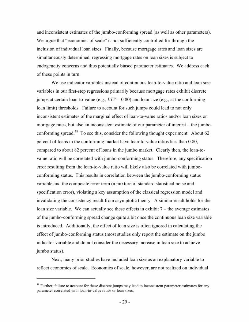
We use the individual mortgage loan data provided by the Mortgage Interest Rate
Survey (MIRS) conducted by the Federal Housing Finance Board. In our data, there are
over one million closed loans from April 1997 through May 2003 (descriptive statistics
are in the upper portion of exhibit 2).13 Because many of the factors affecting mortgage
rates and the jumbo-conforming spread vary by state and time, we run regressions
describing mortgage rates of the individual loan data grouped by state and month of
origination. In particular, we run separate, monthly regressions describing mortgage rates
in four states – California, New Jersey, Maryland, and Virginia – as well as for the
remaining states grouped together. We consider these four states separately because they
have the most developed jumbo loan markets, a relatively high number of jumbo loans
each month, the most jumbo loans over the period of estimation, and no months that
report zero jumbo loans.14 Controlling for state variation in mortgage rates is particularly
important because states have unique laws regarding mortgage origination and
foreclosure laws, which affect the cost of mortgage credit. In addition, the development
of the jumbo mortgage market within states varies substantially because some states have
very high home prices and therefore many homebuyers needing jumbo mortgages,
whereas other states have relatively low home prices and quite limited jumbo markets.
Similar to many previous studies (Henderschott and Shilling, 1989, to Ambrose
and Buttimer, 2004), we regress the mortgage rate of the loan (RM) on a variety of loan
characteristics. The loan-to-value (LTV) information adjusts the mortgage rate for credit
risk.15 Smaller loans (SMALL) are generally more expensive to originate than larger
loans and, for marketing reasons, loans for new home purchases (NEW) are often priced
differently than those for existing homes. In addition, mortgage bankers have a different
cost structure than depository institutions, so we adjust for the type of institution
(MTGCO) that originates the mortgage. Finally, some borrowers pay down their
mortgage rates in the form of up-front fees (FEES), so we control for this mortgage loan
13 We include only 30-year fixed rate mortgages with LTVs between 20 and 97.5 percent and loan sizes between $50,000 and twice the conforming loan limit. 14 Because the MIRS is a voluntary survey, there may be some states that have a substantial jumbo loan market, but few MIRS data reporters. 15 We use four classes of loan-to-value ratios: below 75% (excluded), 75-80%, 81-90%, and above 90%.
- 14 -
characteristic as well.16 We then compare mortgage rates on conforming mortgages
(eligible for purchase by the GSEs) with mortgage rates on jumbo mortgages (ineligible
for purchase by the GSEs because the loan size exceeds the conforming loan limit). The
equation we estimate is
3
0 1 2 3 4 5 6
1
,i
i
RM J LTVi NEW SMALL FEES MTGCOα α α α α α α ε=
= + + + + + + +
for every month and state. The time- and state-varying coefficient on the jumbo loan
indicator variable (J) represents the effect of jumbo status on the mortgage rate.
On average (across states and months), we estimate the jumbo-conforming spread
to be about 16 basis points (upper portion of exhibit 2). In addition, mortgage rates are
generally higher for loans with higher loan-to-value ratios, loans for smaller mortgages17,
loans with up-front fees, and loans originated by mortgage companies. Although the
loan-to-value ratio is the only information on credit worthiness in MIRS, our first-step
regressions explain nearly 77 percent of the variation in mortgage rates.18 The lower-left
panel of exhibit 2 provides a decomposition of our jumbo-conforming spread estimate
across states. The estimated jumbo-conforming spread ranges from about 15 basis points
(in New Jersey) to over 18 basis points (in Maryland). The standard deviations of these
estimates are large, suggesting that the estimated jumbo-conforming spread varies
16 We control for this feature in two ways: first, we use effective mortgage rates (as provided in the MIRS), which amortize the mortgage points and combine them with the mortgage rates, and second, to control for variation that is not accounted for by the amortization process, we use an indicator variable to specify whether or not fees were paid. 17 Note that there is a potential ambiguity here in identifying the jumbo-conforming spread. This is because the “small” variable does not vary independently of the jumbo indicator variable. Thus, what we call the jumbo-conforming spread is really the jumbo to moderately-sized loan spread (in the spirit of Ambrose, Buttimer, and Thibodeau (2001). However, the reason we do this is to capture fixed costs associated with making mortgage loans. Additionally, the coefficient estimate on the “small” variable is about 0.14 – suggesting that the jumbo to small-sized loan spread is only about 2 basis points. Removal of the “small” variable leads to a lower jumbo-conforming spread estimate of about 12 basis points. 18 Note that our “low” estimate of the jumbo-conforming spread is not necessarily due to the lack of information on credit worthiness (outside loan-to-value ratios) in MIRS, as other studies have used MIRS and obtained larger estimates of the jumbo-conforming spread. Instead, we attribute our lower estimate to the later sample (April 1997 through May 2003), which is consistent with trends in the established literature (see, for instance, McKenzie (2002)), and our control for state- and time-specific effects (state-by-state, month-by-month regressions) such as differences in origination and foreclosure laws.
- 15 -
substantially over time.19 The time patterns of the jumbo-conforming spread for the
California and New Jersey markets are presented in the lower-right panel.
Our Analysis of the Jumbo-Conforming Spread
To isolate the effect of the GSE subsidy on mortgage rates, we control for a
variety of factors that influence the jumbo-conforming spread, as estimated by the
coefficients on the jumbo indicator variable in the first-step regressions. As we have
shown, mortgage rates have several major components: The cost of funding the
mortgage (the risk-free cost of funds, RT, and the GSE funding advantage, GA) and the
spreads needed to compensate for the credit (CR), prepayment (PR), and maturity-
mismatch (MR) risks of the mortgage.20,21 Each of these factors could be priced
differently for jumbo mortgages versus conforming mortgages (thereby affecting the
jumbo-conforming spread), especially given the truncated and idiosyncratic nature of the
secondary market for jumbo mortgages. In line with our model, we also include
measures for aggregate demand (DEM), the long-term interest rate (LTRT), and market
capacity (CAP). Finally, we include a time trend to capture any developmental
differences (DEV) between the jumbo and conforming markets and indicator variables for
state (STATE) and quarter (QTR) of origination to capture state and seasonal effects. The
second-step regression we ultimately estimate takes the form
1 0 1 2 3 4 5 6 7
4 3
8 9 10 11
1 1
.s j
s j
s j
GA RT CR PR MR DEM LTRT
CAP DEV STATE QTR
α β β β β β β β β
β β β β η= =
= + + + + + + +
+ + + + +
We proxy for the credit risk spreads associated with conforming mortgages using
the spread between a rate offered on a home equity line of credit (where the combined
loan-to-value of the first and second mortgages cannot exceed 80 percent) and a
19 This should not be confused with statistical significance. The jumbo-conforming spread estimates are generally highly significant. The point is that the jumbo-conforming spread varies substantially over time. 20 Maturity-mismatch risk is the risk that an institution’s liability structure could become out of line with the duration of its assets and that it might be costly to adjust the liabilities to match the asset duration appropriately.21 Interest rate risk is sometimes identified as maturity-mismatch risk and sometimes identified as the combination of this risk and prepayment risk. We will use the more precise language here.
- 16 -
conforming, one-year adjustable rate mortgage.22 Because home equity loans are backed
by second liens and mortgages are backed by first liens, movements in this spread should
partly reflect the small changes in credit risks associated with homeowner delinquency or
default for very safe mortgages.
We compare the daily yield on the current coupon Fannie Mae mortgage-backed
security to a duration-matched yield on AAA/AA financial corporate debt to measure
prepayment risk.23 The maturity-mismatch risk spread is measured as the difference
between the duration-matched corporate yield and the average yield on financial
corporate funding, as weighted by the GSEs’ distribution of debt maturities.24 We use the
one-year Treasury rate to proxy for the risk-free cost of funds and the ten-year Treasury
rate as a measure of the opportunity costs of funding housing (for both portfolio lenders
and households). Our deposit capacity variable is measured as the ratio of total deposits
at banks to total household wealth, while the aggregate mortgage demand variable is
measured as the ratio of total housing wealth to total household wealth.
Our Method for Estimating the GSE Funding Advantage
To calculate the GSE debt advantage, we assume that the GSEs’ long-term debt
advantage is the spread between observed yields on AAA/AA financial corporate debt
and GSE debt, with maturities from one to ten years.25 It is not clear what corporations
are best for this comparison. On one hand, Fannie Mae and Freddie Mac are currently
rated AAA, partly because of their GSE status, and thus one might consider choosing
AAA corporations. On the other hand, without GSE status, the GSEs would be rated
below AAA unless they raised substantial capital or took other actions to offset the loss
22 The rate on the home equity line of credit is from Bank Rate Monitor and the adjustable-rate mortgage rate is from Freddie Mac. 23 These corporate bonds have almost no credit risk. We take the monthly averages for the variables on the right-hand side of the second-step regression. We use Bloomberg’s daily calculation of the MBS current coupon and then match that duration using a daily corporate yield curve for AA/AAA financial corporations to find duration-match values. The daily yield curves are calculated using the technique of Nelson and Siegel (1987), as implemented in Bolder and Stréliski (1999). 24 This is a measure of how far the GSE debt distribution is out of alignment with the current duration of mortgages. 25 We stopped at ten years because there are few comparable corporate debt issues with longer maturities.

- 17 -
of this status.26 Almost all financial corporations, however, find that a AA or A rating is
sufficient; few pursue a AAA rating. In an effort not to overstate the subsidy, we use
AAA/AA financial corporations for our comparison.27
For both GSE and corporate long-term debt, we take the average yield on
outstanding debt grouped by maturity “buckets” (using debt with remaining maturity
from 1 to 3 years, 3 to 5 years, 5 to 7 years, and 7 to 10 years) for each day and then take
the weighted-average of the yields on these four buckets, weighted by the proportion of
GSE debt in each “bucket.” Thus, the maturities on corporate debt outstanding are
adjusted to match GSE maturities.28
As shown in the upper portion of exhibit 3, we create four different indices of
corporate debt spreads, where each index measures liquidity in a slightly different
manner. Our first index uses all 68 firms – regardless of issue size or frequency. The
second index is based on the shear size of the debt issuance. Any issue above $1 billion
is included in this index. There are 15 companies (4 foreign, 11 domestic) in this index.
Here, the assumption is that the size of the debt issue is an important aspect of liquidity.
Our third index is also based on the size of the issue. We include any issue that
exceeds the median size of GSE issues in any given year. In 1997, this issuance
threshold was $165 million. By 2003, it had grown to $696 million. There are 44
companies (11 foreign, 33 domestic) in this index. U.S. investors should be familiar with
these issuers and thus one might assume that these issues are liquid. The fourth index is
based on the debt issuance of GE Capital. Among the financial corporations in our
sample, GE Capital issued debt most frequently and in substantial quantities. As shown
26 Besides the AAA ratings that are based partly on their GSE status, Fannie Mae and Freddie Mac are given “bank financial strength” ratings by Moody’s that assume that GSE status is withdrawn but that there are no other changes that affect the firms (such as changes in agency yields). These ratings are not meant to be compared to Moody’s other credit risk ratings. Fannie Mae and Freddie Mac’s rating of A- is the second-to-best rating and represents the rating Fannie Mae and Freddie Mac would have without GSE status but with no other change in their status (such as their role in the housing system or their funding costs). Nothaft, Pearce, and Stevanovic (2002) state, “We believe the Standard and Poor’s and Moody’s ratings of Freddie Mac and Fannie Mae imply that the relevant comparators for estimating the long-term GSE funding advantage are securities rated AA-.” Fannie Mae’s financial reports also suggest that they manage their business to a AA standard (see FNMA 10-K report, December 31, 2003, page 56). 27 The U.S. Department of the Treasury (1996) used a similar approach but settled on A-rated financial firms for the comparison group, arguing that this rating was common for high-quality financial firms with large portfolios of mortgages. We use Merrill Lynch’s financial corporation data and rely on their classification of corporations. Roughly one-third of the companies are AAA and the remainder are AA. 28 This “bucketing” technique is similar to that used in Sanders (2002).

- 18 -
in the exhibit, the first three measures indicate an average long-term debt advantage of 38
to 44 basis points, with standard deviations between 13 and 18 basis points. The measure
based on GE Capital, however, suggests an average long-term debt advantage of about 24
basis points, with a standard deviation of 14 basis points. We use each of these indices in
our estimation of the GSE funding advantage.
For debt with a maturity of less than one year, we calculate the short-term
advantage as the spread between yields on GSE discount notes and repurchase
agreements using GSE mortgage-backed securities as collateral. We use MBS repos
because Fannie and Freddie hold large amounts of this collateral in their portfolios and
thus could use this market-based funding alternative.29 As shown in the lower-left panel
of exhibit 3, the short-term debt advantage averages about 13 basis points, with a
standard deviation of 6 basis points.
Next, we assume that the GSEs’ mortgage portfolio is effectively funded at the
weighted-average yield on longer-term debt (regardless of whether longer-term debt is
issued and swapped to shorter maturities, shorter-term debt is issued and swapped to
longer maturities, or debt is issued without engaging in a swap) and that the remainder of
GSE assets are funded using short-term debt (the GSEs supposedly issued this debt either
to provide liquidity or to take advantage of short-term arbitrages using their GSE
advantages). This approach assumes that the GSEs’ target debt maturity is the weighted-
average maturity of their stock of debt. Rather than issue all debt at one maturity,
however, they sometimes find it cheaper and less risky (because the tiering of maturities
partly offsets the uncertainty about mortgage prepayments) to issue at other maturities, as
well as engage in swaps. This approach also assumes that the GSEs’ funding advantage
is only the yield difference on debt and is not in the swap transaction (although GSE
status does give the GSEs some advantages with regard to posting collateral for swaps, as
found in Jaffee (2003)). Finally, this approach assumes that the weighted-average yield
captures the effective cost of issuing debt adjusted for the prepayment risks associated
with holding mortgages. Thus, the GSEs’ total debt advantage is the average of these
29 MBS repo rates could themselves embed an implicit subsidy because of the GSE collateralization. We therefore substitute the AA corporate commercial paper rate and find that our results are little changed.
- 19 -
two spreads, weighted by the percent of debt used to fund mortgages.30 As can be seen in
the lower-right panel, the GSEs issued more debt than needed to fund their mortgage
holdings, typically using about 109 percent of the debt needed for funding mortgages.
Regression Analysis
As described earlier, our estimated jumbo-conforming spreads reflect many
different effects besides the GSE advantage. We therefore perform a second-step
regression on the 370 estimates (one estimate for each state and for each month of data)
of the jumbo-conforming spread from the first-step regressions to adjust for certain
factors that influence the spread.31 We include measures for the GSE funding advantage,
mortgage risk characteristics, aggregate mortgage demand, mortgage market capacity, a
time trend to capture development of the market, and dummies for states and quarters to
capture seasonal and region-specific effects (descriptive statistics for these variables are
provided in exhibit 4).
Recalling the second-step regression equation, the fraction of the GSE debt
advantage transmitted to homeowners (the GSE pass-through) is estimated by the
coefficient 1 on the GSE funding advantage variable (GA). Because we have four
proxies for corporate yields (each reflecting a slightly different concept of corporate debt
liquidity), we estimate our model four times, resulting in four (different) estimates of the
pass-through from the GSEs’ gross debt advantage to homeowners’ mortgage rates. We
use all four proxies to preserve each source of variation. Including each proxy in a single
estimation poses interpretation problems, so we instead opt to estimate each specification
separately, and then apply minimum distance estimation to calculate the mortgage rate
savings to homeowners.
The upper portion of exhibit 5 contains our estimates for each regression. Note
that the reported standard errors are corrected for heteroskedasticity, first-order
autocorrelation, and clustering by month. Without such corrections, estimated standard
30 This approach is similar to CBO (2001), which assumed that the GSEs’ optimal mix was 80 percent long-term (greater than one year) and 20 percent short-term (less than one year). This approach effectively treats callable debt and some short-term debt (the portion swapped to have longer maturities) the same as longer-term “plain-vanilla” debt. 31 In sensitivity analysis described later, we also use the difference between monthly average jumbo and conforming mortgage rates as a measure of the jumbo-conforming spread.

- 20 -
errors would be 30-40 percent smaller. Also, note that the GSE funding advantage has a
statistically significant positive effect on the jumbo-conforming spread in only two of the
four cases, conditional on other important factors, such as credit, prepayment, and
funding risks, funding costs, and regional factors.32 As expected, our regression results
indicate that the jumbo-conforming spread widens when mortgage demand is high or
when deposit capacity is low, and tightens as the mortgage market becomes more
developed. Each source of risk (credit, prepayment, and maturity-mismatch) also appears
to price differently across the jumbo and conforming markets, with the higher pricing
occurring in the less-developed jumbo sector of the mortgage market (though not to a
statistically significant degree).
In order to reconcile our differing estimates of the GSE pass-through, we use
minimum distance estimation. The minimum distance estimator takes an implicit
weighted average of the parameter estimates according to some criteria function. We
minimize the quadratic form of the standardized difference between the minimum
distance estimate and the four parameter estimates
( ) ( )*
* 1 *
ˆ
ˆ ˆ ˆ ˆˆmin ,β
β β β β−′− Ω −
where β is the vector of preliminary GSE pass-through estimates, *β is the minimum
distance estimator of the pass-through, and Ω is the variance-covariance matrix for β
which explicitly accounts for any correlation among the proxy variables. Because we
minimize this particular criteria function, our weighting is a function of the variance-
covariance terms. We report these implicit weights along with the underlying parameter
estimates in exhibit 5.
The minimum distance estimator results in a point estimate of about 16.4 percent
for the GSE pass-through. The lower panel of exhibit 5 shows our estimate of the
32 Due to our formulation of some of the explanatory variables, 78-85 percent of the variation in GA is explained by the other regressors. However, testing for multicollinearity is much akin to testing for micronumerosity – or small n (Goldberger, 1991, ch. 23). Moreover, as Goldberger (1991, p. 252) points out, “To say that ‘standard errors are inflated by multicollinearity’ is to suggest that they are artificially, or spuriously, large. But in fact they are appropriately large: the coefficient estimates actually would vary a lot from sample to sample. This may be regrettable but it is not spurious.” Further, the same process that leads to large standard errors also leads to large (not small) coefficient estimates, in particular the coefficient on GA.

- 21 -
asymptotic distribution of the minimum distance estimator of the GSE pass-through. As
shown in the exhibit, the median pass-through is about 16.4 percent and the 95-percent
confidence interval runs from -1.6 percent to 34.5 percent. Also, our four preliminary
pass-through estimates (dashed lines), ranging from 6.6 to 31.0 percent, span the
weighted average and lie within the 95-percent confidence interval.
Mortgage Rate Savings
As shown in the upper panel of exhibit 6, we calculate that yields on Fannie and
Freddie’s long-term debt run about 42 basis points lower than those for our comparison
group, with a standard deviation of 13 basis points. To calculate the long-term
advantage, we use a weighted average of our four GSE debt advantage indexes. The
weights are each index’s contribution to the minimum distance estimator of the GSE
pass-through, discussed below. That is, let ˆiβ denote the ith index’s estimate of the GSE
pass-through and let *β denote the minimum distance estimate of the GSE pass-through.
Then the predicted jumbo-conforming spread using the four indexes is
4
1
ˆˆi i i
i
y w x β=
=
where iw is the ith index’s weight and ix is the ith index’s GSE debt advantage. The
hypothetical jumbo-conforming spread using the minimum distance estimator is
* * *ˆy x β=
where we do not observe *x . We therefore substitute y in for *y and solve for *x – a
weighted average of the ix s – so that
4* *
1
ˆ ˆˆ / .i i i
i
x w x β β=
=
This is an estimate of the GSE debt advantage consistent with our minimum distance
estimate of the GSE pass-through. In contrast, the estimated GSE advantage from issuing
short-term debt averages 13 basis points, with a standard deviation of 6 basis points. As
shown in the middle panel, we estimate that the overall GSE advantage averaged about
40 basis points during the past decade, with a standard deviation of 12 basis points.
- 22 -
For our calculation of the mortgage rate savings to homeowners, we use our pass-
through estimate of 16.4 percent and our weighted-average estimate of the GSE debt
advantage. As shown in the lower panel of exhibit 6, this implies that GSE activities
typically account for about 6.5 basis points of the difference between jumbo and
conforming mortgage rates, with an estimated standard deviation of 1.9 basis points.
5. Sensitivity Analysis and Interpreting Our Regressions
As the reader may know, Fannie Mae (2004) and Raines (2004) have commented
on our approach in several respects, including our use of a discrete loan-to-value variable,
our decision not to include a continuous loan size variable, our limited ability to control
for subprime mortgages, and our comparison of GSE funding costs to private
corporations instead of swaps. In addition, in two studies sponsored by Fannie Mae,
Greene (2004) and Blinder (2004) raise concerns about the robustness and efficiency of
our estimates.33 We deal with each of these concerns by implementing several alternative
specifications. As we show, our results are robust to these alternative specifications – the
estimated mortgage rate reduction attributed to these GSEs does not generally increase
and may very well be smaller (see exhibits 7-8).
California Only
As discussed earlier, the MIRS data has a variety of problems. However, the
more recent data for California, which has the largest and most complete jumbo market,
may avoid some of the problems encountered when using the nationwide data. Thus, we
first explore the sensitivity of our results to estimation on this subsample of our data. The
average estimate (over time) of the jumbo-conforming spread is a bit larger in the
California subsample (17.1 basis points) than in the full sample (16.2 basis points). The
minimum distance estimate of the pass-through is also a bit larger in the California
subsample (20.8 percent) than in the full sample (16.4 percent). Based on an average
33 In another study commissioned by Fannie Mae, Blinder, Flannery, and Kamihachi (2004) provide a comprehensive critique of our methodology, including additional sensitivity analysis and alternative interpretations of our theoretical and empirical models. Our response to their study is contained in Passmore and Sherlund (2005). We show that the results of this paper are, largely, quite consistent with the results obtained by Blinder, Flannery, and Kamihachi.

- 23 -
weighted GSE debt advantage of 37.9 basis points, we estimate the mortgage rate
reduction to be 7.9 basis points for the California subsample. Although a bit larger, this
is not statistically different from the estimated mortgage rate reduction of 6.5 basis points
using the full sample.
Measuring Loan-to-Value Ratios
Second, Fannie Mae (2004) raises concerns about our use of discrete loan-to-
value variables. In lieu of the indicator variables employed in our original specification,
we use the continuous loan-to-value ratio, as provided by the MIRS. The average jumbo-
conforming spread is now estimated to be only 14.8 basis points and the minimum
distance estimate of the GSE pass-through is 16.7 percent. Based on the average
weighted GSE debt advantage of 38.9 basis points, we estimate the mortgage rate
reduction to be 6.5 basis points – virtually identical to the results of our original
specification.
Adding Loan Size as an Explanatory Variable
Many researchers have used loan size as an explanatory variable in the first-step
regression, even though such a variable is clearly simultaneously determined with
mortgage rates. Moreover, researchers rarely adjust their measure of the jumbo-
conforming spread for its interaction with the loan size variable. We will discuss whether
loan size should be included as an explanatory variable in the following section. Here,
we focus on how to interpret the results correctly once loan size is included in the first-
step regression. Fannie Mae (2004) presents estimates of the jumbo-conforming spread
using loan size as an explanatory variable. Indeed, one can show that the average
treatment effect, or the jumbo-conforming spread in this case, is just the conditional
difference between average mortgage rates in the jumbo and conforming markets. This is
exactly what the model without the continuous loan size variable estimates. When one
includes the loan size as an explanatory variable, the resulting estimate of the jumbo-
conforming spread essentially double counts the decrease in mortgage rates arising
because of a larger loan size, which must then be subtracted off to calculate the average
treatment effect of jumbo-conforming status.

- 24 -
When we introduce loan size as an additional explanatory variable in the first-step
regressions, the average estimate of the coefficient on the jumbo-conforming dummy
under this specification increases substantially to 27.8 basis points. However, when we
account for the double counting described above, the estimate of the jumbo-conforming
spread for average conforming versus average jumbo mortgages is still 16.2 basis points
(the end results, therefore, are identical to those of our original specification). However,
erroneously using the coefficient on the jumbo dummy instead of the corrected measure
for the jumbo-conforming spread yields a minimum distance estimate of the GSE pass-
through of only 7.8 percent. Multiplied by the average weighted GSE debt advantage of
42.4 basis points gives an estimated mortgage rate reduction of only 3.3 basis points. The
decrease in the estimated GSE pass-through under this approach more than offsets the
perceived increase in the estimated coefficient on the jumbo dummy variable.
Controlling for Subprime Mortgages
To control for the possible presence of subprime mortgage loans in our data, we
first restrict our sample to contain only mortgage loans with loan-to-value ratios less than
or equal to 80 percent. This approach yields an estimated jumbo-conforming spread of
14.4 basis points and a minimum distance pass-through estimate of 10.6 percent. The
average weighted GSE debt advantage is 42.5 basis points, implying an estimated
mortgage rate reduction of 4.5 basis points. This estimate is lower than, but not
statistically different from, the estimate from our original specification.
Next, taking a more direct approach to control for possible subprime loans, we
treat any non-jumbo mortgage with a mortgage rate in the top ten percent of non-jumbo
mortgage rates as subprime by including an indicator variable in the first-step
regressions.34 This method increases the estimated jumbo-conforming spread to 22.7
basis points, but the minimum distance estimate of the pass-through decreases to 13.8
percent. The average weighted GSE debt advantage is 38.6 basis points, implying an
34 The MIRS survey is voluntary and the Federal Housing Finance Board, which runs the survey, does not make public the institutions that participate. However, given the history of the survey, it seems unlikely that it includes any subprime lenders.
- 25 -
estimated mortgage rate reduction of 5.3 basis points. Once again, this is not statistically
different from the results of our original specification.
Taking a different approach, we treat any mortgage loan with a spread to the 10-
year Treasury rate of 300 basis points or more as subprime by including an indicator
variable in the first-step regressions. The average jumbo-conforming spread under this
approach is 13.9 basis points and the minimum distance estimate of the GSE pass-
through is 11.3 percent. Multiplied by the average weighted GSE debt advantage of 41.0
basis points gives an estimated mortgage rate reduction of 4.6 basis points. As before,
this point estimate is not statistically different from that of our original specification.
Interpreting the Jumbo-Conforming Dummy Variable
Greene (2004) raises several concerns with the econometric specification and
techniques we employ. First, he cites an ambiguity in measuring the jumbo-conforming
spread. In our regression analysis, we include indicator variables for both jumbo loans
and for smaller loans (with principal balances less than $100,000). The estimated
coefficients on these two indicator variables therefore reflect the premium (or discount)
in pricing these types of loans relative to moderately-sized (neither small nor jumbo)
loans. Our average estimate of the coefficient on the jumbo loan indicator variable is
about 16 basis points – which we call the jumbo-conforming spread, since it measures the
pricing difference between moderately-sized and jumbo loans.
Greene correctly points out, however, that an ambiguity arises because of the
inclusion of the small loan indicator variable. If we want to compare small loans with
jumbo loans, we need to take into account not only the estimated effect of jumbo status,
but the effect of small-loan status as well. Our average estimate of the coefficient on the
small loan indicator variable is 14 basis points indicating that small loans cost, on
average, 14 basis points more than comparable moderately-sized loans, implying that the
jumbo-conforming spread for small loans is only 2 basis points. Thus, for a generic
conforming loan (either small or moderately-sized) the jumbo-conforming spread lies
between 2 and 16 basis points. We believe that comparing moderately-sized loans to
jumbo loans gives a better comparison for understanding the effect of GSEs, mainly
because generally higher small loan rates might reflect diseconomies of scale.

- 26 -
Inefficiency and Two-Step Estimation
Greene also cites potential bias and inefficiency in estimation that may lead to
“seriously flawed results.” Efficiency is not an argument about whether or not our
coefficients are accurate, but instead about the effective use of the information provided
within the sample. We argue that our estimates are not necessarily inefficient given the
underlying data structure. We conduct what is called multilevel data analysis – analysis
on some data that are micro-level (individual loans) and other data that are macro-level
(monthly macro variables). In this context, all that is needed in terms of efficiency, we
believe, is large group sizes (number of loans per month) and a relatively small number
of groups (total number of months), both of which are satisfied with the MIRS data.35
Greene seems to believe that our econometric specification focuses on the first-
step equation and therefore falls within a random coefficients framework. Instead, our
analysis actually focuses on the second-step equation, in which estimates of the jumbo-
conforming spread are regressed against the GSE debt advantage and other variables
reflecting risk and economic conditions. This equation requires some estimate of the
jumbo-conforming spread, which, in our analysis, we derive from the first-step
estimation.
However, to address the concern with potential bias and inefficiency due to two-
step estimation (Greene, 2004), we calculate the jumbo-conforming spread as the
difference between mean jumbo and conforming mortgage rates for each month and state
and include monthly averages of the first-step explanatory variables as additional
explanatory variables in estimating the second-step regression – thereby avoiding the
first-step regressions altogether. The average jumbo-conforming spread under this
approach is 12.7 basis points and the minimum distance pass-through estimate is 13.6
percent. Multiplying by the average weighted GSE debt advantage of 36.9 basis points
leads to a mean mortgage rate reduction of 5.0 basis points. Again, our original
specification seems robust to this alternative specification and estimation methodology.
35 Note that we already adjust our standard errors to account for heteroskedasticity, first-order autocorrelation, and clustering by month.

- 27 -
Interpreting the GSE Implicit Subsidy Pass-Through to Mortgage Rates
Blinder (2004) discusses the random component to estimation, i.e., the range of
parameter estimates implied by standard errors, which underlies all economic analysis.
In particular, he is concerned that “the range of uncertainty is large.” However, the range
of uncertainty is not large enough for us to believe that the GSEs’ entire implicit subsidy
is passed through to mortgage rates. Our estimate of the GSE pass-through is 16.4
percent, with a standard error of 9.2 percentage points. We can therefore easily reject the
hypothesis that the implied subsidy is passed through in its entirety to homeowners via
reduced mortgage rates. Note, however, that we cannot reject the hypothesis that none of
the subsidy is passed through to homeowners at conventional confidence levels.
Blinder also argues that the GSE funding advantage is not a product of the
implicit subsidy alone, that the jumbo-conforming spread is not due to the GSE funding
advantage alone, and that homeownership rates are not only affected through mortgage
rates. Our estimation attempts to control for economies of scale and efficiency found in
the conforming MBS market (to remove this effect from the GSE funding advantage) and
models the jumbo-conforming spread as not only a function of the GSE debt advantage,
but other variables as well, to account for the GSEs’ business operations and overall
economic conditions. We agree with Blinder that one must try to distinguish between the
mortgage rate reductions generated by the business operations of an effective and
efficient mortgage securitizer from those generated by the GSE subsidy.
Debt Advantage Relative to Swap Yields
Fannie Mae (2004) suggested that the GSE funding advantage be measured by
comparing their funding costs to the swap yield curve. The swap yield curve, however,
does not represent any particular institution’s funding costs, particularly over a long time
horizon. The swap yield curve is derived from three month LIBOR. For example, the
10-year swap yield is the yield one could expect to pay if one could issue three-month
debt at LIBOR regularly at three-month intervals over the next ten years. The British
Banker’s Association computes LIBOR, which represents the unsecured debt costs at
- 28 -
short maturities of an average bank in the Association’s panel.36 The criteria for
inclusion in the panel are not public, but a bank must have a high credit standing and be a
major participant in interbank cash and forward markets. Bank of America, Citibank, and
JP Morgan Chase are American banks that are currently included in the panel.
Using data from Lehman, we construct spread to swap series for Bank of America
(BAC), Wells Fargo (WFC), and Fannie Mae (FNM) for January 2001 through May
2003. These series, along with the jumbo-conforming spread, are depicted in the upper
panel of exhibit 9. As shown, Fannie Mae’s funding advantage relative to swaps first
became negative in 2001 and then again in 2002. Bank of America and Wells Fargo had
much larger spreads to swaps than Fannie Mae did.
We consider regressions of two forms: One using the corporate-swap and swap-
agency spreads as distinct explanatory variables, and the other using the corporate-agency
spread.37 Each regression also controls for risk and pricing characteristics, as in our
original analysis. As shown in exhibit 9, the swap-agency spread has a much larger
effect than the corporate-swap spread on the jumbo-conforming spread, though both
effects are statistically indistinguishable from zero (but different from one) at
conventional confidence levels. The corporate-agency spread also has a statistically
negligible impact on the jumbo-conforming spread.
These results suggest that Fannie Mae may indeed price mortgages as a spread to
swaps. However, this spread does not capture the debt advantage resulting from the
implicit subsidy and therefore is not the proper comparison to make. When we do draw
the proper comparison, we find that little or none of the debt advantage is passed through
to homeowners in the form of lower mortgage rates.
A Note on Specification of the First-Step Regressions
Because mortgage rates exhibit discrete jumps at various loan-to-value and loan
size thresholds, we show that inclusion of a continuous variable itself may lead to biased
36 The “U.S. Dollar” panel contains 16 banks. The banks report their funding costs at 11:00 a.m. each day. The yields reported by the highest four and lowest four banks are thrown out and the yields of the middle eight banks are averaged to create “LIBOR.” 37 We do not use only the swap-agency spread because this ignores the bulk of the implicit subsidy. We therefore include the corporate-swap spread as an additional explanatory variable.
- 29 -
and inconsistent estimates of the jumbo-conforming spread (as well as other parameters).
We argue that “economies of scale” is not sufficiently controlled for through the
inclusion of individual loan sizes. Finally, because mortgage rates and loan sizes are
simultaneously determined, regressing mortgage rates on loan sizes is subject to
endogeneity concerns and thus potentially biased parameter estimates. We address each
of these points in turn.
We use indicator variables instead of continuous loan-to-value ratio and loan size
variables in our first-step regressions primarily because mortgage rates exhibit discrete
jumps at certain loan-to-value (e.g., LTV = 0.80) and loan size (e.g., at the conforming
loan limit) thresholds. Failure to account for such jumps could lead to not only
inconsistent estimates of the marginal effect of loan-to-value ratios and/or loan sizes on
mortgage rates, but also an inconsistent estimate of our parameter of interest – the jumbo-
conforming spread.38 To see this, consider the following thought experiment. About 62
percent of loans in the conforming market have loan-to-value ratios less than 0.80,
compared to about 82 percent of loans in the jumbo market. Clearly then, the loan-to-
value ratio will be correlated with jumbo-conforming status. Therefore, any specification
error resulting from the loan-to-value ratio will likely also be correlated with jumbo-
conforming status. This results in correlation between the jumbo-conforming status
variable and the composite error term (a mixture of standard statistical noise and
specification error), violating a key assumption of the classical regression model and
invalidating the consistency result from asymptotic theory. A similar result holds for the
loan size variable. We can actually see these effects in exhibit 7 – the average estimates
of the jumbo-conforming spread change quite a bit once the continuous loan size variable
is introduced. Additionally, the effect of loan size is often ignored in calculating the
effect of jumbo-conforming status (most studies only report the estimate on the jumbo
indicator variable and do not consider the necessary increase in loan size to achieve
jumbo status).
Next, many prior studies have included loan size as an explanatory variable to
reflect economies of scale. Economies of scale, however, are not realized on individual
38 Further, failure to account for these discrete jumps may lead to inconsistent parameter estimates for any parameter correlated with loan-to-value ratios or loan sizes.

- 30 -
loan sizes (do originators really line up borrowers and start with the smallest loan sizes?)
– instead, they are realized at the aggregate margin. We control for this aspect in the
second step of our analysis, allowing economies of scale to differ between the jumbo and
conforming markets, through aggregate demand and market development variables and,
to some extent, the state- and time-specific intercept terms in the first-step regressions.
Further, the traditional modeling of economies of scale requires the inclusion of not only
loan size, but higher-order terms of loan size as explanatory variables.
Finally, putting aside our two prior points, loan size is an endogenous variable.
Therefore, including loan size as an explanatory variable (without instrumentation) leads
to biased and inconsistent parameter estimates. We therefore take a dual approach –
considering input and output prices instead of loan size (much akin to estimating cost or
profit functions instead of production functions in production analysis). One could think
of the dual approach as a reduced-form regression, with input and output prices acting as
instruments for the loan size. We include input and output prices in the second-step
regression, in which we estimate the effects of input prices on the jumbo-conforming
spread.
6. Conclusions
In this paper, we derive a theoretical model of how jumbo and conforming
mortgage rates are determined and how the jumbo-conforming spread might arise. We
show that mortgage rates reflect the cost of funding mortgages and that this cost of
funding can drive a wedge between jumbo and conforming rates (the jumbo-conforming
spread) because the two markets may have different funding costs. Further, we show
how the jumbo-conforming spread tightens when mortgage demand is low, core deposits
are sufficient to fund mortgage demand, and as the mortgage market become more liquid
and realizes economies of scale.
Using MIRS data for April 1997 through May 2003, we estimate the jumbo-
conforming spread to be 15-18 basis points. Further, we find that GSEs pass through
only about 16 percent of their 40 basis point debt advantage, lowering homeowners’
mortgage rates by 7 basis points. This result provides evidence that the jumbo-
conforming spread provides only an upper bound for the amount that GSEs lower

- 31 -
mortgage rates. That is, the GSE funding advantage accounts for 7 basis points of the 15-
18 basis point jumbo-conforming spread.

- 32 -
References
Ambrose, B. and R. Buttimer (2004). “GSE Impact on Rural Mortgage Markets,” Regional Science and Urban Economics, forthcoming.
Ambrose, B., R. Buttimer, and T. Thibodeau (2001). “A New Spin on the Jumbo-Conforming Loan Rate Differential,” Journal of Real Estate Finance and Economics, 23, 309-336.
Ambrose, B., M. LaCour-Little, and A. Sanders (2002). “The Effect of Conforming Loan Status on Mortgage Yield Spreads: A Loan Level Analysis,” mimeo from authors,November 3, 2003.
Ambrose, B. and T. Thibodeau (2004). “Have the GSE Affordable Housing Goals Increased the Supply of Mortgage Credit,” Regional Science and Urban Economics, 34, 263-273.
Blinder, A.S. (2004). Letter on Federal Reserve Working Paper to CEO Raines from Dr.
Alan S. Blinder.
Blinder, A.S., M.J. Flannery, and J.D. Kamihachi (2004). “The Value of Housing-Related Government Sponsored Enterprises: A Review of a Preliminary Draft Paper by Wayne Passmore,” Fannie Mae.
Bolder, D. and D. Stréliski (1999). “Yield Curve Modeling at the Bank of Canada,” Technical Report No. 84, Bank of Canada.
Congressional Budget Office (2001). Federal Subsidies and the Housing GSEs,Washington, D.C.: Government Printing Office.
Cotterman, R. and J. Pearce (1996). “The Effects of the Federal National Mortgage Association and the Federal Home Loan Mortgage Corporation on Conventional Fixed-Rate Mortgage Yields” in Studies on Privatizing Fannie Mae and Freddie Mac,Washington, D.C.: U.S. Department of Housing and Urban Development, 97-168.
Fannie Mae (2004). Preliminary Response to Wayne Passmore Federal Reserve Working
Paper: ‘The GSE Implicit Subsidy and Value of Government Ambiguity.’
Goldberger, A.S. (1991). A Course in Econometrics, Cambridge, MA: Harvard University Press.
Goodman, J.L., Jr., and W. Passmore (1992). “Market Power and the Pricing of Mortgage Securitization,” Federal Reserve Board Finance and Economics Discussion
Series, 187, 1-31.

- 33 -
Greene, W.H. (2004). Commentary on ‘The GSE Implicit Subsidy and Value of
Government Ambiguity.’
Hendershott, P. and J. Shilling (1989). “The Impact of Agencies on Conventional Fixed-Rate Mortgage Yields,” Journal of Real Estate Finance and Economics, 2, 101-115.
Hermalin, B. and D. Jaffee (1996). “The Privatization of Fannie Mae and Freddie Mac: Implications for Mortgage Industry Structure,” in Studies on Privatizing Fannie Mae and
Freddie Mac, Washington, D.C.: U.S. Department of Housing and Urban Development, 225-302.
Heuson, A., W. Passmore, and R. Sparks (2001). “Credit Scoring and Mortgage Securitization: Implications for Mortgage Rates and Credit Availability,” Journal of Real
Estate Finance and Economics, 23, 337-364.
Jaffee, D. (2003). “The Interest Rate Risk of Fannie Mae and Freddie Mac,” Journal of
Financial Services Research, 24, 5-29.
McKenzie, J. (2002). “A Reconsideration of the Jumbo/Non-Jumbo Mortgage Rate Differential,” Journal of Real Estate Finance and Economics, 25, 197-213.
Mankiw, N.G. (2003). Remarks at the Conference of State Bank Supervisors, State Banking Summit and Leadership Conference, November 6, 2003.
Naranjo, A. and A. Toevs (2002). “The Effects of Purchases of Mortgages and Securitization by Government Sponsored Enterprises on Mortgage Yield Spreads and Volatility,” Journal of Real Estate Finance and Economics, 25, 173-196.
Nelson, C. and A. Siegel (1987). “Parsimonious Modeling of Yield Curves,” Journal of
Business, 60, 473-489.
Nothaft, F., J. Pearce, and S. Stevanovic (2002). “Debt Spreads Between GSEs and Other Corporations,” Journal of Real Estate Finance and Economics, 25, 151-172.
Passmore, W. and S.M. Sherlund (2005). “GSE Subsidy Transmission in Competitive Banking Markets,” forthcoming.
Passmore, W. and R. Sparks (1996). “Putting the Squeeze on a Market for Lemons: Government-Sponsored Mortgage Securitization,” Journal of Real Estate Finance and
Economics, 13, 27-43.
Passmore, W. and R. Sparks (2000). “Automated Underwriting and the Profitability of Mortgage Securitization,” Journal of Real Estate Finance and Economics, 28, 285-305.
Passmore, W., R. Sparks, and J. Ingpen (2002). “GSEs, Mortgage Rates and Mortgage Securitization,” Journal of Real Estate Finance and Economics, 25, 215-242.

- 34 -
Raines, F.D. (2004). Testimony before U.S. Committee on Banking, Housing, and Urban Affairs, February 25, 2004.
Sanders, A. (2002). “Government Sponsored Agencies: Do the Benefits Outweigh the Costs?” Journal of Real Estate Economics, 25, 121-127.
Torregrosa, D. (2001). “Interest Rate Differentials Between Jumbo and Conforming Mortgages, 1995-2000,” Congressional Budget Office.
U.S. Department of the Treasury (1996). Government Sponsorship of the Federal
National Mortgage Association and the Federal Home Loan Mortgage Corporation,Washington, D.C.: Government Printing Office.

Exhibit 1
The Jumbo-Conforming Spread
rMJ 45o
M rMC
C B A
Jumbo
Market
Bank Low Cost
Conforming Bank High Cost
Market Mortgage Bankers
45o M Demand
rMJ
Projection of supply 45o
onto rMC-rM
J space
rMJ,H C
DH
rMJ,M B
DM
rMJ,L A
DL
rMC
rMC,L
rMC,M
rMC,H
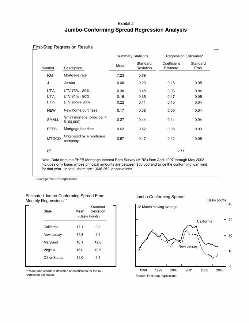
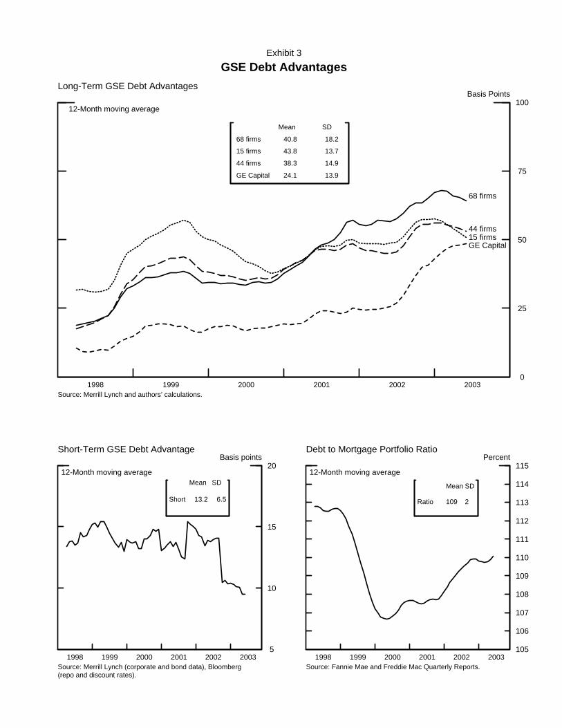
1998 1999 2000 2001 2002 2003 0
25
50
75
100Basis Points
Source: Merrill Lynch and authors’ calculations.
Long-Term GSE Debt Advantages
12-Month moving average
15 firms44 firms
68 firms
GE Capital
Mean SD
68 firms 40.8 18.2
15 firms 43.8 13.7
44 firms 38.3 14.9
GE Capital 24.1 13.9
1998 1999 2000 2001 2002 2003 5
10
15
20Basis points
Source: Merrill Lynch (corporate and bond data), Bloomberg(repo and discount rates).
Short-Term GSE Debt Advantage
12-Month moving averageMean SD
Short 13.2 6.5
1998 1999 2000 2001 2002 2003105
106
107
108
109
110
111
112
113
114
115Percent
Source: Fannie Mae and Freddie Mac Quarterly Reports.
Debt to Mortgage Portfolio Ratio
12-Month moving average
Mean SD
Ratio 109 2
Exhibit 3
GSE Debt Advantages

Exhibit 4
Variables Used in Regression Analysis
Symbol Description
1 0.16 0.10
GA68 0.40 0.16
GA15 0.43 0.12
GA44 0.37 0.13
GAGE 0.23 0.13
RT 4.29 1.65
CR 1.93 0.89
PR 0.78 0.33
MR68 0.21 0.18
MR15 0.11 0.26
MR44 0.21 0.19
MRGE 0.35 0.19
DEM 0.16 0.02
LTRT 5.33 0.78
CAP 0.01 0.00
DEV 0.38 0.21
S1 0.20 0.40
S2 0.20 0.40
S3 0.20 0.40
S4 0.20 0.40
QTR1 0.24 0.43
QTR2 0.27 0.44
QTR3 0.24 0.43
Credit risk
Mean
Summary Statistics
GSE funding advantage (GE Capital)
GSE funding advantage (15 firms)
Prepayment risk
Maturity-mismatch risk (GE Capital)
Standard
Deviation
Maturity-mismatch risk (44 firms)
GSE funding advantage (44 firms)
One year treasury rate
JC Spread
GSE funding advantage (68 firms)
Virginia
Maryland
Mortgage market capacity
Aggregate mortgage demand
Ten year treasury rate
New Jersey
Quarter 3
Quarter 1
Quarter 2
Mortgage market development
California
Maturity-mismatch risk (15 firms)
Maturity-mismatch risk (68 firms)

1998 1999 2000 2001 2002 2003 0
10
20
30
40
50
60
70
80Basis points
Source: Merrill Lynch (corporate and bond data), Bloomberg (repo and discount rates).
GSE Debt Advantage by Parts
12-Month moving average
Long-TermAdvantage
Short-Term Advantage
Mean SD
Long 42.0 13.1
Short 13.2 6.5
1998 1999 2000 2001 2002 200310
15
20
25
30
35
40
45
50
55
60Basis points
Source: Merrill Lynch, Bloomberg.
GSE Weighted Debt Advantage
12-Month moving average Mean SD
Debt 39.5 11.9
1998 1999 2000 2001 2002 2003 2
4
6
8
10
12Basis points
Source: Merrill Lynch and second-step regressions.
Estimated GSE Mortgage Rate Reductions
12-Month moving averageMean SD
MortgageRate Reduction
6.5 1.9
Exhibit 6
Mortgage Rate Reduction

Exhib
it 7
Se
ns
itiv
ity
An
aly
sis
Ke
y R
esults
16.2
17.1
14.8
27.8
14.4
22.7
13.9
12.7
Sta
ndard
devia
tion
10.3
9.3
10.3
12.7
9.8
10.8
8.9
11.5
16.4
20.8
16.7
7.8
10.6
13.8
11.3
13.6
Sta
ndard
err
or
9.2
9.4
9.3
10.1
9.0
9.7
8.2
9.4
6.5
7.9
6.5
3.3
4.5
5.3
4.6
5.0
Sta
ndard
Devia
tion
1.9
2.8
2.0
0.9
1.2
1.7
1.3
1.8
6.6
11.3
6.8
-4.2
0.6
6.2
-1.9
9.7
Sta
ndard
Err
or
10.9
11.2
10.9
11.9
10.9
11.4
10.4
10.2
31.0
39.9
31.4
18.4
22.8
29.4
19.9
25.3
Sta
ndard
Err
or
11.2
13.2
11.2
11.2
10.5
12.1
9.4
11.8
16.6
27.7
17.0
7.6
7.6
15.7
6.3
17.0
Sta
ndard
Err
or
9.9
10.5
9.8
11.1
10.3
10.2
10.3
9.8
9.9
17.4
9.8
2.3
1.2
7.0
5.2
10.9
Sta
ndard
Err
or
11.3
12.7
11.1
12.7
10.9
11.9
10.5
11.1
--
----
----
----
----
----
S
pecific
ation --
----
----
----
----
----
--
----
----
-- S
ubprim
e --
----
----
--
Subprim
e
10-y
ear
+
300 b
ps
Month
ly
Avera
ges
GE
Capital
Min
imum
dis
tance p
ass-t
hro
ugh e
stim
ate
Mean jum
bo-c
onfo
rmin
g s
pre
ad
Mean m
ort
gage r
ate
reduction
68 firm
s
15 firm
s
Pre
limin
ary
Pass-t
hro
ugh E
stim
ate
s
Origin
al
Subprim
e
Top 1
0%
Loan S
ize
44 firm
s
Calif
orn
ia
Continuous
LT
Vs
LT
V
80%
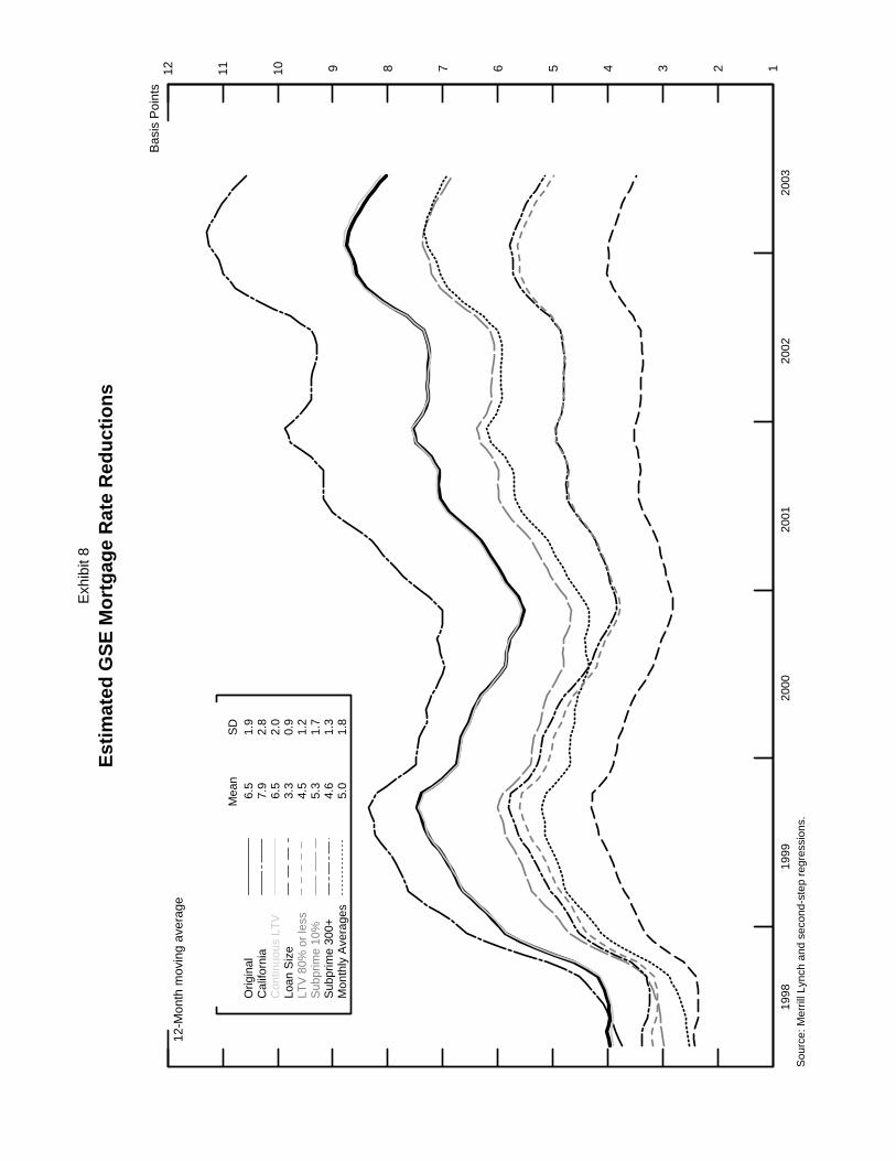
1998
1999
2000
2001
2002
2003
1 2 3 4 5 6 7 8 9101112B
asis
Poi
nts
Sou
rce:
Mer
rill L
ynch
and
sec
ond-
step
reg
ress
ions
.
12-M
onth
mov
ing
aver
age
Mea
nS
DO
rigin
al6.
51.
9C
alifo
rnia
7.9
2.8
Con
tinuo
us L
TV
6.5
2.0
Loan
Siz
e3.
30.
9LT
V 8
0% o
r le
ss4.
51.
2S
ubpr
ime
10%
5.3
1.7
Sub
prim
e 30
0+4.
61.
3M
onth
ly A
vera
ges
5.0
1.8
Exh
ibit
8
Est
imat
ed G
SE
Mo
rtg
age
Rat
e R
edu
ctio
ns


