

The Fermilab Photo-Injector
Jean-Paul Carneiro (Fermilab & Université Paris XI)For the A0 group (N. Barov, M. Champion, D. Edwards, H. Edwards,
J. Fuerst, W. Hartung, M. Kuchnir, J. Santucci)
Accelerator Physics and Technology Seminars Fermilab, March 23, 2001
OUTLINE
1. Introduction: R&D on linear colliders e+/e- at Fermilab NLC, TESLA2. Layout of the A0 Photo-Injector3. Experiments Dark current Quantum efficiency Transverse emittance Bunch length Compression User experiments5. Conclusion
NLC: 30 km long, copper cavities, 1 TeV COM, luminosity ~1110-33 cm-2 s-1. Collaboration Fermilab/SLAC.
TESLA: 30 km long, superconducting cavities, 0.8 TeV COM, luminosity ~27.510-33 cm-2 s-1. Collaboration between 9 countries and 41 institutions.
R&D on linear colliders e+/e- at Fermilab
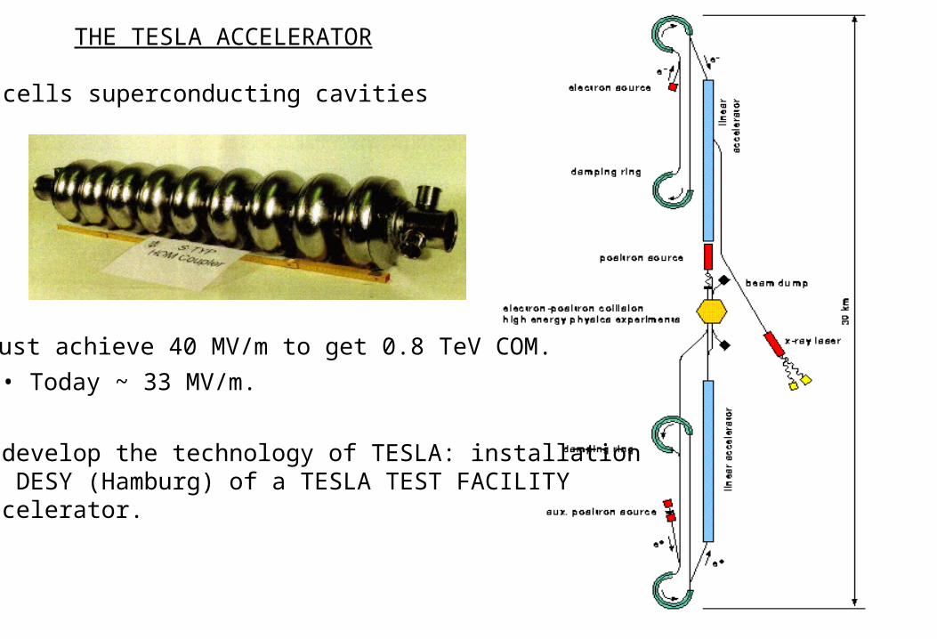
THE TESLA ACCELERATOR
• 9-cells superconducting cavities
• Must achieve 40 MV/m to get 0.8 TeV COM.
• Today ~ 33 MV/m.
• To develop the technology of TESLA: installation at DESY (Hamburg) of a TESLA TEST FACILITY accelerator.

THE TESLA TEST FACILITY ACCELERATOR
~ 100 meters
• Fermilab contribution to TTF : - design, fabrication and commissioning of the TTF injector (Nov 98).
- design and prototyping of RF couplers for the cavities. - design and prototyping of long-pulse modulators for the klystrons.

THE TESLA TEST FACILITY ACCELERATOR

THE TESLA TEST FACILITY PHOTO-INJECTOR

THE TTF ONDULATO R
• Self-Amplified Spontaneous Emission observed at 209 nm in February 2000.
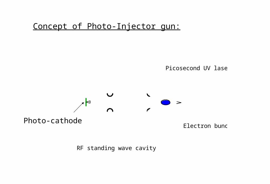
RF standing wave cavity
Electron bunch
Picosecond UV laser
Concept of Photo-Injector gun:
Photo-cathode
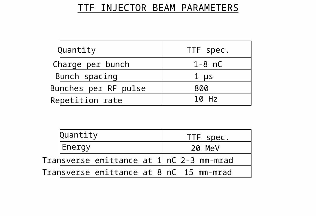
TTF INJECTOR BEAM PARAMETERS
Quantity
Charge per bunch
Bunch spacing
Bunches per RF pulse
Repetition rate
TTF spec.
1-8 nC
1 µs
800 10 Hz
Quantity
Energy
Transverse emittance at 1 nC
Transverse emittance at 8 nC
TTF spec.20 MeV
2-3 mm-mrad
15 mm-mrad
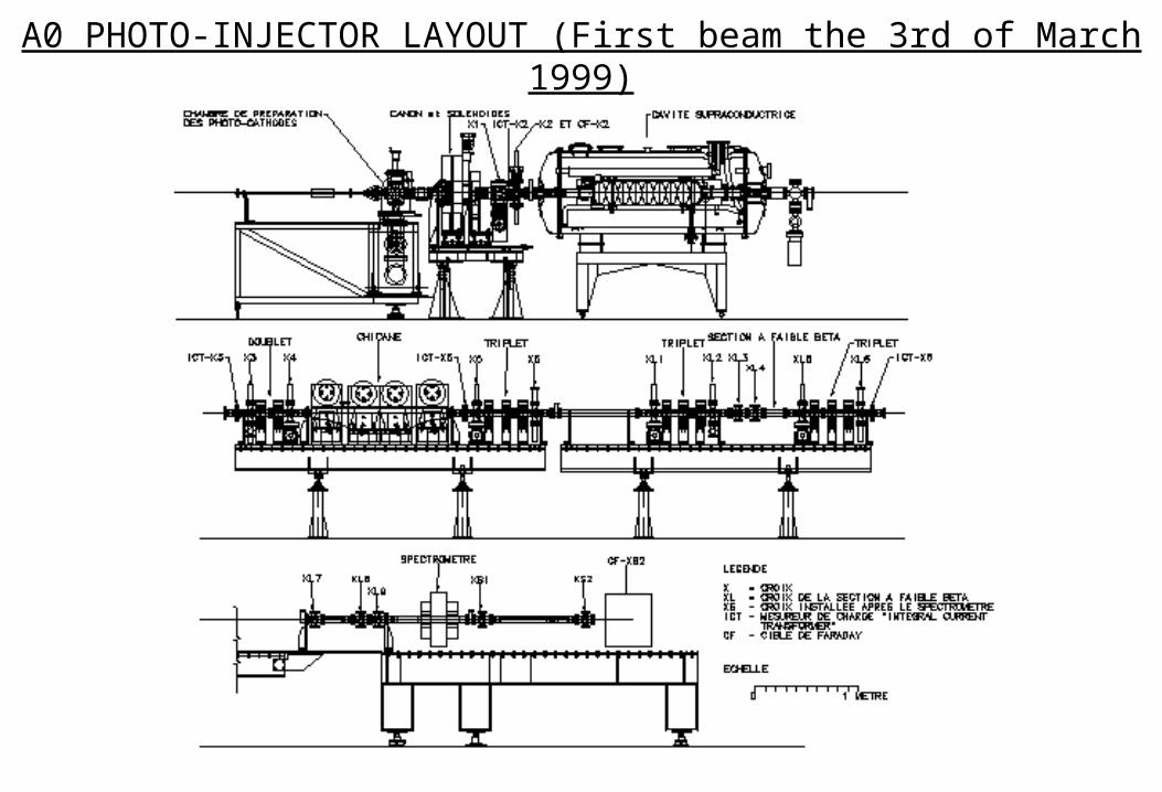
A0 PHOTO-INJECTOR LAYOUT (First beam the 3rd of March 1999)

Oscillator Nd:YLF81.25 MHz
2 km optic fiber Pockels Cell1 MHz
Multi-pass amplifierNd-glass
Double-pass amplifierNd-glass
12 nJ/pulse60 ps
1054 nm
2.5 nJ/pulse400 ps
800 pulses2 nJ/pulse
400 ps
100 µJ/pulse400 ps
0.8 mJ/pulse400 ps
600 µJ/pulse400 ps
400 µJ/pulse4.2 ps
100 µJ/pulse4.2 ps
532 nm
20 µJ/pulse4.2 ps
263 nm
10 µJ/pulse10.8 ps263 nm
LASER (University of Rochester)
STACKED UNSTACKED
Spatial filterCompressorBBO CrystalsPulse stacker
0
5
10
15
20
25
0 10 20 30 40 50 602
4
6
8
10
12
0 5 10 15 20 25 30
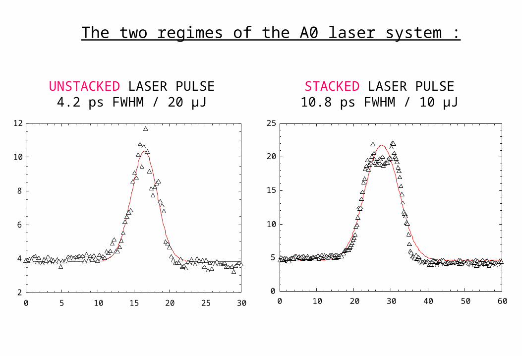
UNSTACKED LASER PULSE4.2 ps FWHM / 20 µJ
STACKED LASER PULSE10.8 ps FWHM / 10 µJ
The two regimes of the A0 laser system :

THE PHOTO-CATHODE PREPARATION CHAMBER (INFN-Milano)
• Coat Mo cathodes with a layer of Cs2Te, a material of high quantum efficiency (QE).
• Use manipulator arms to transfer the cathode from the preparation chamber into the RF gun while remaining in UHV.
• Cathodes must remain in ultra-high vacuum (UHV) for its entire useful life, because residual gases degrade the QE. • Contamination can be reversed by rejuvenation: heat cathode to ~230 C for some minutes.
• The same cathode has been used in the RF gun for ~2 years without degradation of its QE (~0.5-3%)

BUCKING SOLENOID
PRIMARY SOLENOID
SECONDARY SOLENOID
THE RF GUN AND SOLENOIDS (Fermilab & UCLA)
• RF gun and solenoids developed by Fermilab and UCLA.
ModeResonant frequency
Peak fieldTotal energyPeak power dissipationPulse lengthRepetition rateAverage power dissipationCooling water flow rate
TM010,π
4.5 MeV2.2 MW800 µs10 Hz28 kW
35 MV/m
4 L/s
Q 240001.3 GHz
Gun parameters
Solenoids parameters
• Bucking & Primary max. Bz --> 2059 G (385A)• Secondary max. Bz --> 806 G (312 A)
• 1.5-cell copper cavity designed for a high duty cycle (0.8%).
RF GUN
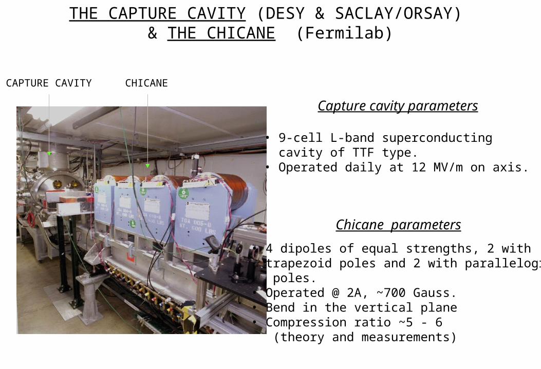
THE CAPTURE CAVITY (DESY & SACLAY/ORSAY) & THE CHICANE (Fermilab)
CHICANECAPTURE CAVITY
Capture cavity parameters
Chicane parameters
• 9-cell L-band superconducting cavity of TTF type.• Operated daily at 12 MV/m on axis.
• 4 dipoles of equal strengths, 2 with trapezoid poles and 2 with parallelogram poles.• Operated @ 2A, ~700 Gauss.• Bend in the vertical plane• Compression ratio ~5 - 6 (theory and measurements)

THE LOW BETA SECTION THE WHOLE BEAMLINE
SPECTROMETER
EXPERIMENTPLASMA WAKEFIELD ACCELERATION

DARK CURRENT STUDIES
Idc
150
Vdtt
150
91710 9
60 10 60.3 mA
X2 Faraday Cup Oscilloscope trace
channel 1 Forward power into the gun
channel 2 Faraday Cup X2 signal
•Dark current measurement principle : Using a Faraday Cup at X2 (z~0.6 m).
Bucking Ib
Primary Ip
Secondary Is

Comparison of Dark current : March 99 / November 00
0
0.5
1
1.5
2
2.5
3
3.5
0 10 20 30 40 50
03/04/99 Ib=I
p=I
s=0 A
02/11/00 Ib=I
p=I
s=220 A
02/11/00 Ib=I
p=I
s=0 A
RF gun peak field [MV/m]
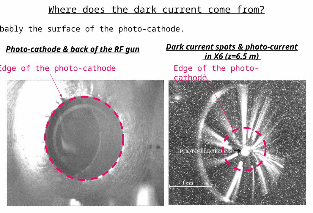
Edge of the photo-cathode Edge of the photo-cathode
Where does the dark current come from?
•Probably the surface of the photo-cathode.
Photo-cathode & back of the RF gun Dark current spots & photo-current in X6 (z=6.5 m)
0.25
0.3
0.35
0.4
0.45
0.5
0.55
0.6
0 1 2 3 4 5 6 7 8
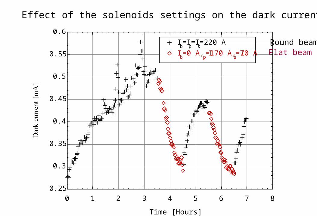
Ib=I
p=I
s=220 A
Ib=0 A, I
p=170 A, I
s=70 A
Time [Hours]
Round beamFlat beam
Effect of the solenoids settings on the dark current
1
1.1
1.2
1.3
1.4
1.5
1.6
1.7
1.8
1 10-9
2 10-9
3 10-9
4 10-9
5 10-9
6 10-9
7 10-9
8 10-9
9 10-9
0 100 200 300 400 500
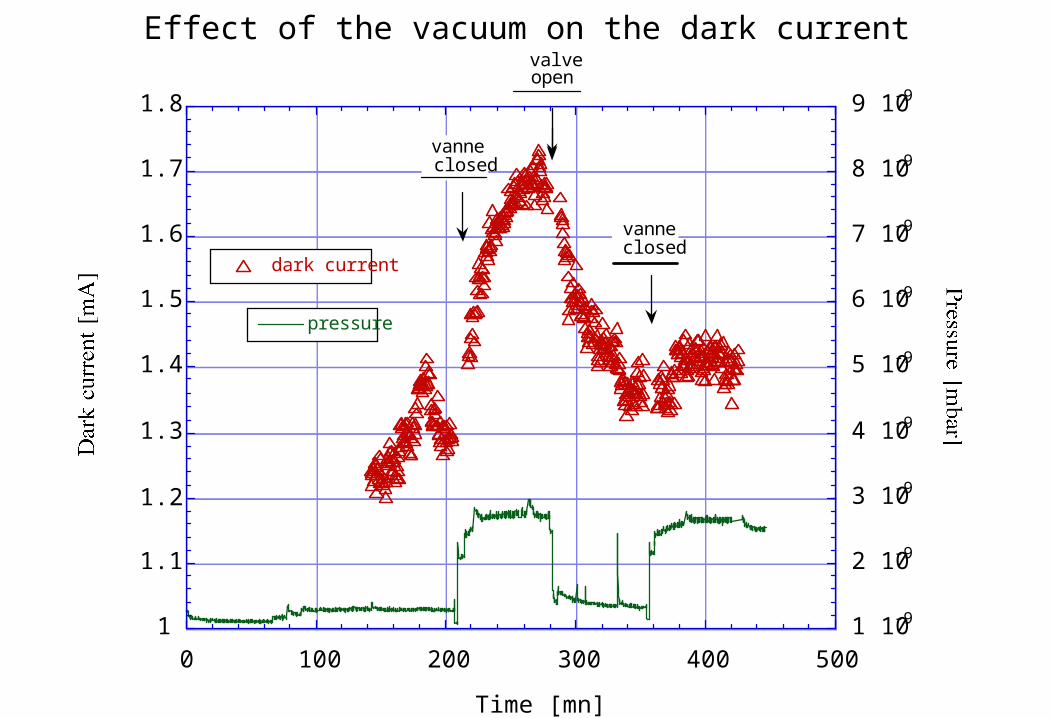
dark current
pressure
Time [mn]
vanne closed
valveopen
vanneclosed
Effect of the vacuum on the dark current
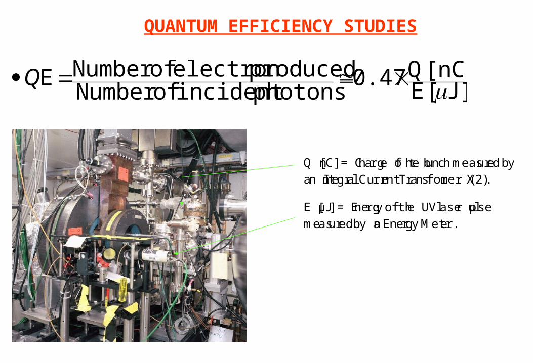
QUANTUM EFFICIENCY STUDIES
QENumberof electron producedNumberof incident photons
0.47Q[nC]E[J]
Q [nC] = Charge of the bunch measured byan Integral Current Transformer (X2).
E [µJ] = Energy of the UV laser pulsemeasured by an Energy Meter.

0.3
0.4
0.5
0.6
0.7
0.8
0.9
1
1.1
0 1 2 3 4 5 6
Ib=0 A, I
p=170 A, I
s=70 A
Ib=I
p=I
s=220 A
Time [Hour]
Round beamFlat beam
Effect of the solenoids settings on the Quantum Efficiency
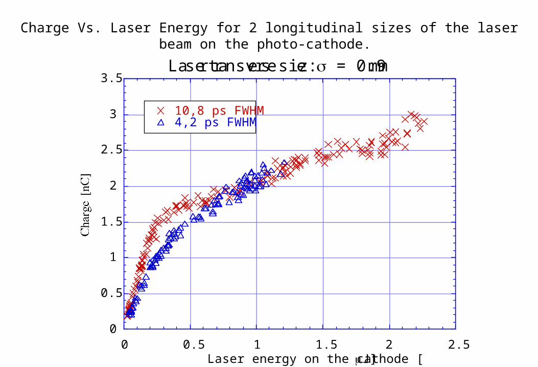
0
0.5
1
1.5
2
2.5
3
3.5
0 0.5 1 1.5 2 2.5
10,8 ps FWHM4,2 ps FWHM
Laser energy on the cathode [J]
Charge Vs. Laser Energy for 2 longitudinal sizes of the laser beam on the photo-cathode.
Laser transverse size : = 0.9 mm
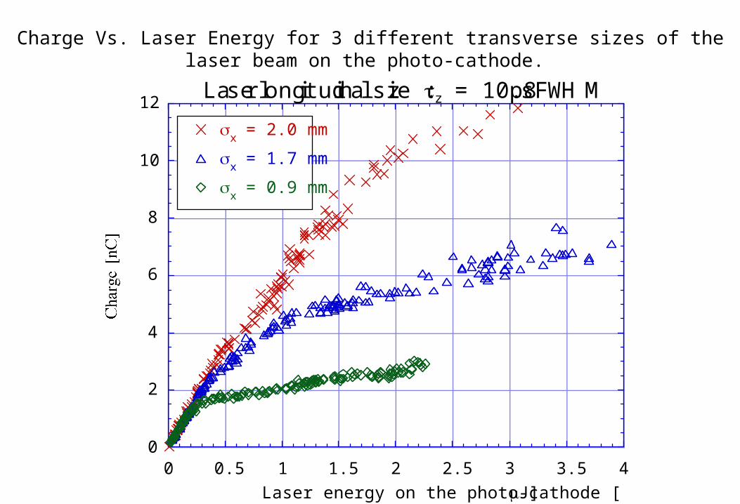
0
2
4
6
8
10
12
0 0.5 1 1.5 2 2.5 3 3.5 4
x = 2.0 mm
x = 1.7 mm
x = 0.9 mm
Laser energy on the photo-cathode [J]
Charge Vs. Laser Energy for 3 different transverse sizes of the laser beam on the photo-cathode.
Laser longitudinal size : z = 10.8 ps FWHM

0
1
2
3
4
5
6
0 0.5 1 1.5 2 2.5 3 3.5
MeasurementFit with Gauss law (Hartman model, UCLA)
Laser energy on the cathode[J]
Charge Vs. Laser Energy for = 0.8 mm on the photo-cathode.
(Hartman, NIM A340, p.219-230, 1994)

TRANSVERSE EMITTANCE MEASUREMENTS
Q = Charge of the bunch (laser energy)
r = Laser pulse transverse size
z = Laser pulse length
E0 = Peak field on RF gun
0 = Launch phase
Ib, Ip, Is = Current in the solenoids
Ecc = Capture cavity accelerating field
cc = Capture cavity RF phase
Laser
RF Gun
CaptureCavity
• The photo-injector is a set of 8 parameters:
• Goal: find for a charge Q, the set of parameters that gives the min. transverse emittance.• Remark: for all the emittance measurements, the chicane was OFF and DEGAUSSED.
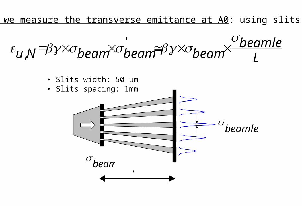
• How do we measure the transverse emittance at A0: using slits
u,N beambeam' beam
beamletL
L
• Slits width: 50 µm• Slits spacing: 1mm
beam
beamlet
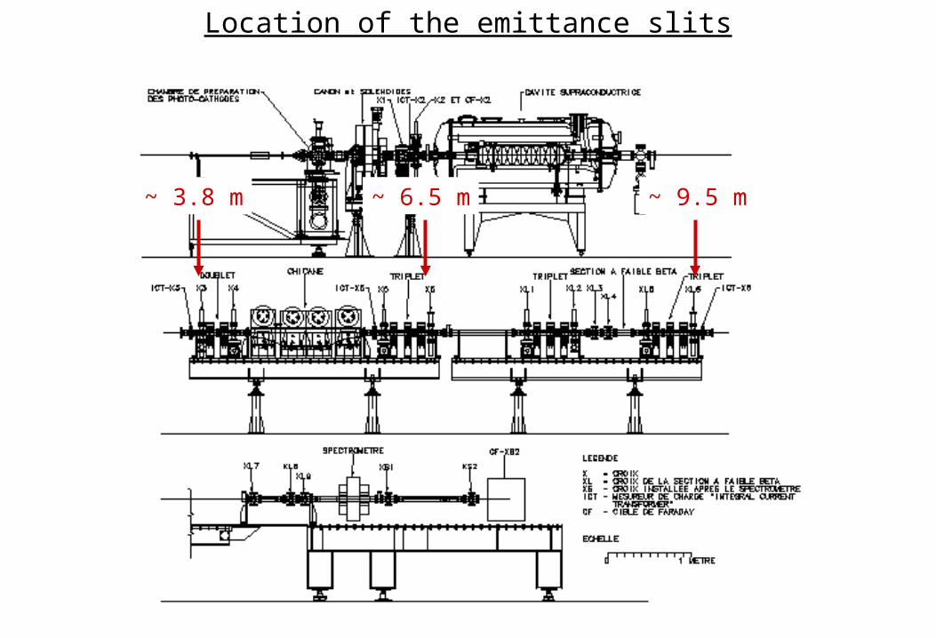
Location of the emittance slits
~ 3.8 m ~ 9.5 m~ 6.5 m

10
20
30
40
50
60
70
0 2 4 6 8 10 12
u,N
beam
beam'
18
0.511
1.8 mm 70.8 m
384 mm
11.7 mm mrad
80
100
120
140
160
0 2 4 6 8 10 12 14 Position [mm]Position [mm]
beam
1.8 mm beamlet
70.8 m
Inte
nsit
y [
a. u
.]
Inte
nsit
y [
a. u
.]
Example: emittance measurement of 8 nC in X3 (z~3.8 m), beamlets in X4 (∆z = 384 mm)
BEAM X3 BEAMLETS X4

Ecc = 12 MV/m
cc = at the minimum of energy spread
z = 10.8 ps FWHM
1/ For a fixed charge Q (0.25, 1, 4, 6, 8 and 12 nC), we
tried to find the set of 4 parameters (0, E0, Isol, r) to
obtain the minimum transverse emittance at z=3.8 m.
2/ We measured the emittance at z=6.5 m and z=9.4 m.
3/ We compared the results with 2 codes of simulation
PARMELA (V5.03 from Orsay, B. Mouton)
Known code, slow execution (~15 Hours).
HOMDYN ( HTWA21 from Frascati, M. Ferrario)
New code, fast execution (~2-3 minutes).
How did we proceed with the emittance measurements ?
FIXED PARAMETERS

1.5
2
2.5
3
3.5
4
4.5
0 100
1 102
2 102
3 102
4 102
5 102
6 102
-100 -50 0 50 100 150 200 250 300
Transmission before experimentTransmission after experiment
Launch phase [Deg]
Emittance Vs. Launch Phase (z=3.8 m)
Q=1 nC, E0=35 MV/m,=0.8 mm
øo=40 deg
Q=0.4 nC
Q=0.5 nC
Q=0.8 nC
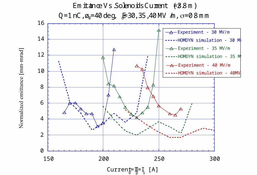
0
2
4
6
8
10
12
14
16
150 200 250 300
Experiment - 40 MV/m
HOMDYN simulation - 40MV/m
Experiment - 35 MV/m
HOMDYN simulation - 35 MV/m
Experiment - 30 MV/m
HOMDYN simulation - 30 MV/m
Current Ib=I
p=I
s [A]
Emittance Vs. Solenoids Current (z=3.8 m)
Q=1 nC, ø0=40 deg, Eo=30, 35, 40 MV/m, =0.8 mm

10
15
20
25
30
35
40
45
140 160 180 200 220 240 260 280
Current Ib=I
p=I
s
10
15
20
25
30
35
40
45
140 160 180 200 220 240 260 280
Experiment - 30 MV/m
HOMDYN simulation - 30 MV/m
Experiment - 40 MV/m
HOMDYN simulation - 40 MV/m
Experiment - 35 MV/m
HOMDYN simulation - 35 MV/m
E0 = 40 MV/m
Emittance Vs. Solenoids Current (z=3.8 m)
Q=8 nC, ø0=40 deg, Eo=30, 35, 40 MV/m, =1.6 mm

0
1
2
3
4
5
6
150 200 250 300 350
HOMDYN simulation
PARMELA simulation
Measurement (x = 0.4 mm)
Current Ib=I
p=I
s [A]
Emittance Vs. Solenoids Current (z=3.8 m)
Q=0.25 nC, ø0=40 deg, Eo=40 MV/m, =0.4 mm
Min Emit @ 205 A
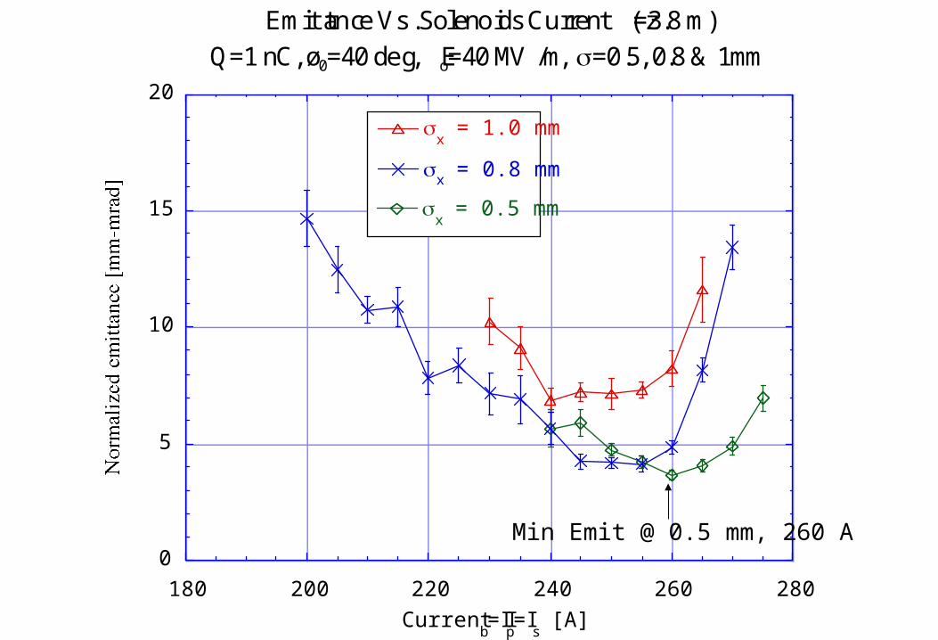
0
5
10
15
20
180 200 220 240 260 280
x = 1.0 mm
x = 0.5 mm
x = 0.8 mm
Current Ib=I
p=I
s [A]
Emittance Vs. Solenoids Current (z=3.8 m)
Q=1 nC, ø0=40 deg, Eo=40 MV/m, =0.5, 0.8 & 1mm
Min Emit @ 0.5 mm, 260 A

0
5
10
15
20
180 200 220 240 260 280 300
Measurement (x = 0.5 mm)
HOMDYN simulation
PARMELA simulation
Current Ib=I
p=I
s [A]
Comparison Measurements / HOMDYN / PARMELA
Case Q=1nC, =0.5 mm

0
10
20
30
40
50
210 220 230 240 250 260 270 280 290
x = 1.5 mm
x = 1.2 mm
x = 1.8 mm
Current Ib=I
p=I
s [A]
Emittance Vs. Solenoids Current (z=3.8 m)
Q=4nC, ø0=40 deg, Eo=40 MV/m, =1.2, 1.5 & 1.8 mm
Min Emit @ 1.2 mm, 260 A

5
10
15
20
25
30
35
40
45
180 200 220 240 260 280 300 320
PARMELA simulation
HOMDYN simulation
Measurement (x = 1.2 mm)
Current Ib=I
p=I
s [A]
Comparison Measurements / HOMDYN / PARMELA
Case Q=4 nC, =1.2 mm
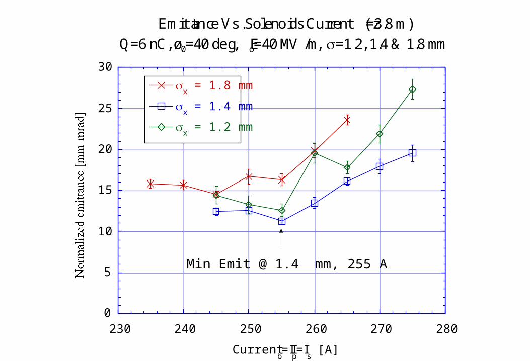
0
5
10
15
20
25
30
230 240 250 260 270 280
x = 1.8 mm
x = 1.4 mm
x = 1.2 mm
Current Ib=I
p=I
s [A]
Emittance Vs. Solenoids Current (z=3.8 m)
Q=6 nC, ø0=40 deg, Eo=40 MV/m, =1.2, 1.4 & 1.8 mm
Min Emit @ 1.4 mm, 255 A
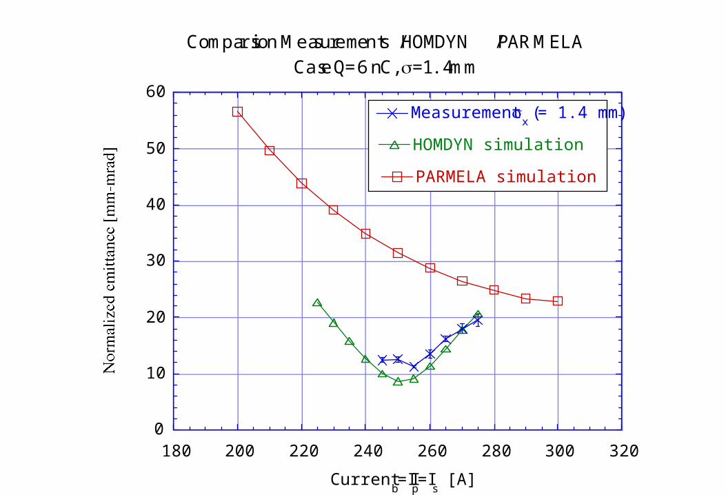
0
10
20
30
40
50
60
180 200 220 240 260 280 300 320
HOMDYN simulation
PARMELA simulation
Measurement (x = 1.4 mm)
Current Ib=I
p=I
s [A]
Comparison Measurements / HOMDYN / PARMELA
Case Q=6 nC, =1.4 mm
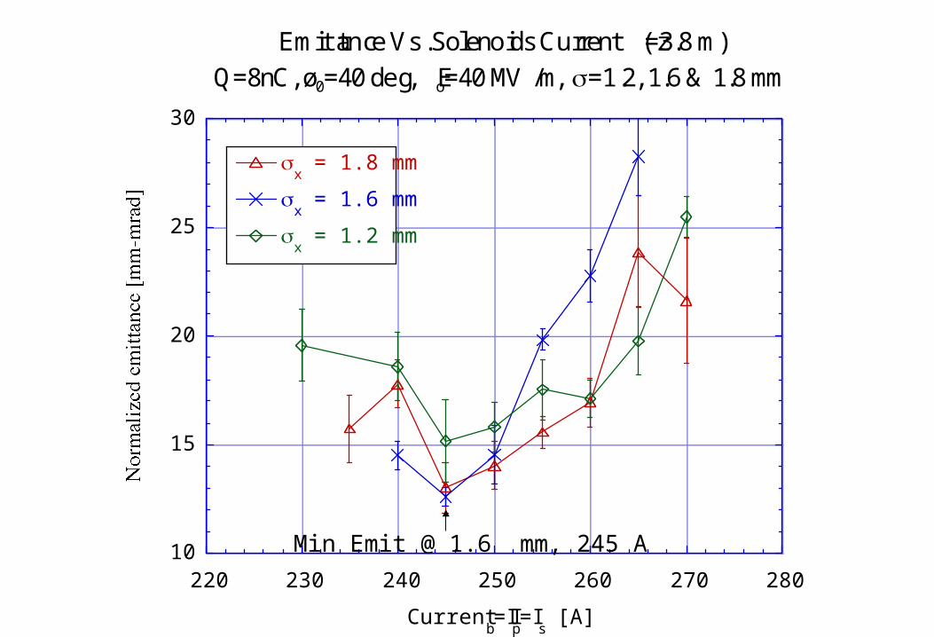
10
15
20
25
30
220 230 240 250 260 270 280
x = 1.8 mm
x = 1.6 mm
x = 1.2 mm
Current Ib=I
p=I
s [A]
Emittance Vs. Solenoids Current (z=3.8 m)
Q=8nC, ø0=40 deg, Eo=40 MV/m, =1.2, 1.6 & 1.8 mm
Min Emit @ 1.6 mm, 245 A
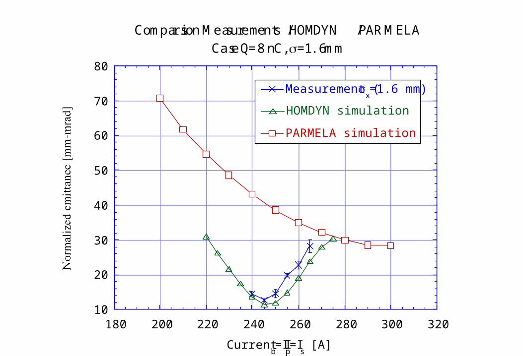
10
20
30
40
50
60
70
80
180 200 220 240 260 280 300 320
Measurement (x=1.6 mm)
HOMDYN simulation
PARMELA simulation
Current Ib=I
p=I
s [A]
Comparison Measurements / HOMDYN / PARMELA
Case Q=8 nC, =1.6 mm

0
20
40
60
80
100
180 200 220 240 260 280 300 320
Measurement (x = 2.1 mm)
HOMDYN simulation
PARMELA simulation
Current Ib=I
p=I
s [A]
Emittance Vs. Solenoids Current (z=3.8 m)
Q=12 nC, ø0=40 deg, Eo=40 MV/m, =2.1 mm
Min Emit @ 2.1 mm, 225 A
0
10
20
30
40
50
60
70
80
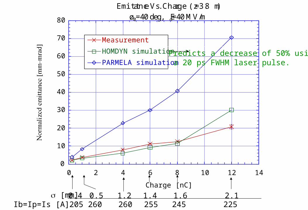
0 2 4 6 8 10 12 14
Measurement
HOMDYN simulation
PARMELA simulation
Charge [nC]
[mm]Ib=Ip=Is [A]
0.4 0.5 1.2 1.4 1.6 2.1205 260 260 255 245 225
Emittance Vs. Charge (z=3.8 m)
ø0=40 deg, Eo=40 MV/m
Predicts a decrease of 50% using a 20 ps FWHM laser pulse.

0
0.5
1
1.5
2
2.5
3
3.5
4
0 2 4 6 8 10 12
Measurement (x)
Measurement (y)
HOMDYN simulation (x)
HOMDYN simulation (y)
PARMELA simulation (x)
PARMELA simulation (y)
Longitudinal position [m]
Beam envelope for Q=1 nC.
ø0=40 deg, Eo=40 MV/m, =0.8 mm, Ib=Ip=Is=255 A.
Q3=1.32 A, Q4=-2.42 A, Q5=1.32 A.
6.5 m9.4 m

0
2
4
6
8
10
0 2 4 6 8 10 12
HOMDYN simulation (x)
HOMDYN simulation (y)
PARMELA simulation (x)
PARMELA simulation (y)
Longitudinal position [m]
Beam envelope for Q=8 nC.
ø0=40 deg, Eo=40 MV/m, =1.6 mm, Ib=Ip=Is=245 A.
Q3=1.3 A, Q4=-2.6 A, Q5=1.3 A & Q6=2.2 A, Q7=-4.2 A, Q8=2.2 A.
6.5 m 9.4 m
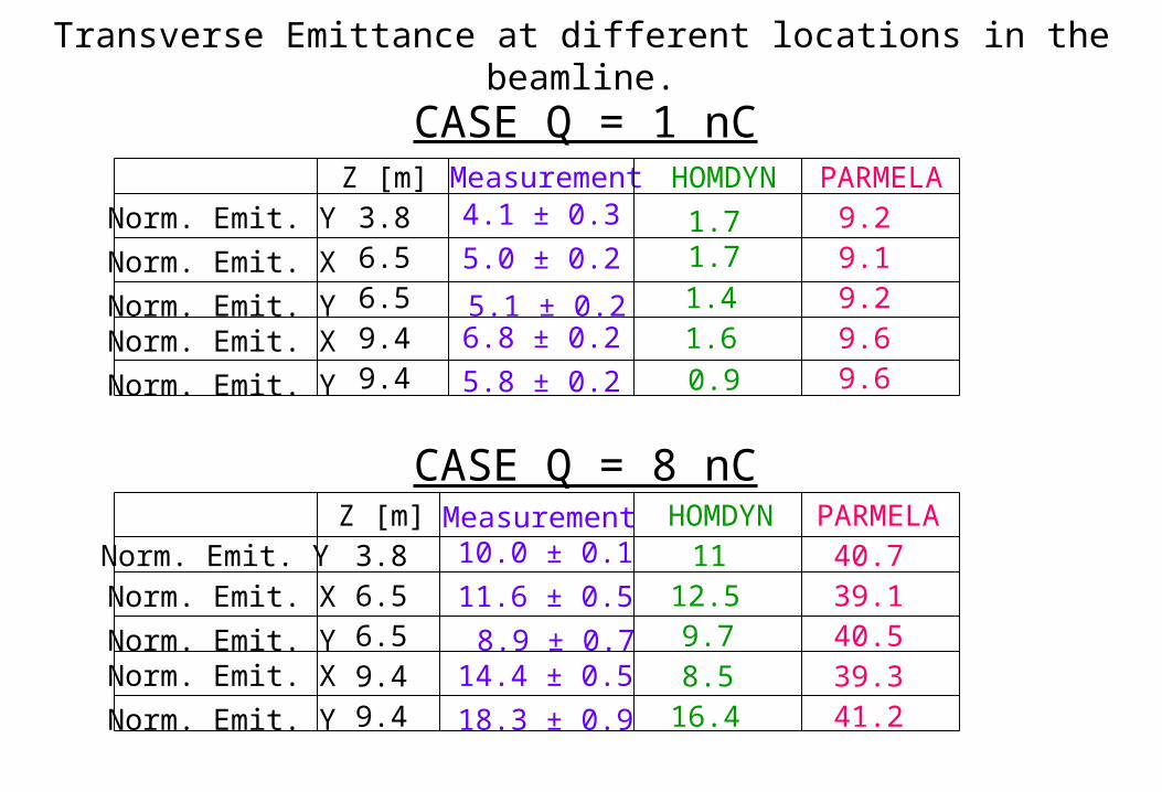
Norm. Emit. Y Z [m] HOMDYN PARMELA
3.8 11 40.76.5 12.5 39.16.5 9.7 40.59.4 8.5 39.39.4 16.4 41.2
10.0 ± 0.1
11.6 ± 0.5
8.9 ± 0.714.4 ± 0.5
18.3 ± 0.9
Z [m] Measurement HOMDYN PARMELA3.8 1.7 9.26.5 1.7 9.16.5 1.4 9.29.4 1.6 9.69.4 0.9 9.6
4.1 ± 0.3
5.0 ± 0.2
5.1 ± 0.26.8 ± 0.2
5.8 ± 0.2
CASE Q = 1 nC
CASE Q = 8 nC
Norm. Emit. Y
Norm. Emit. X
Norm. Emit. YNorm. Emit. X
Norm. Emit. Y
Norm. Emit. X
Norm. Emit. YNorm. Emit. X
Norm. Emit. Y
Measurement
Transverse Emittance at different locations in the beamline.
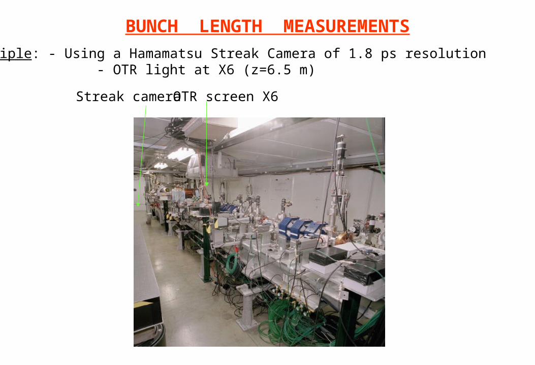
BUNCH LENGTH MEASUREMENTS
• Principle: - Using a Hamamatsu Streak Camera of 1.8 ps resolution - OTR light at X6 (z=6.5 m)
Streak camera OTR screen X6
18
20
22
24
26
28
30
0 0.5 1 1.5 2 2.5 3 3.5 4127.5
128
128.5
129
129.5
130
130.5
131
131.5
0 20 40 60 80 100
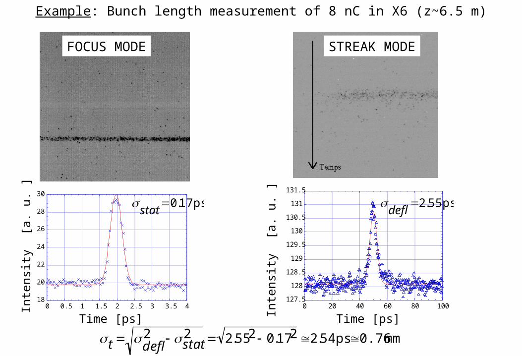
stat
0.17 ps defl
2.55 ps
Time [ps] Time [ps]
Inte
nsit
y [
a. u
. ]
Inte
nsit
y [
a. u
. ]
FOCUS MODE STREAK MODE
t defl2 stat
2 2.552 0.172 2.54 ps 0.76 mm
Example: Bunch length measurement of 8 nC in X6 (z~6.5 m)
0
0.5
1
1.5
2
2.5
3
3.5
4
0 2 4 6 8 10 12
Parmela simulation
Homdyn simulation
Measurement
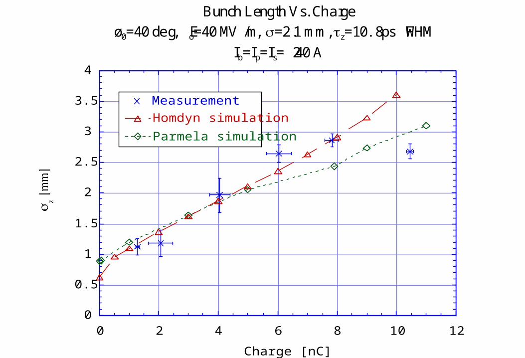
Charge [nC]
Bunch Length Vs. Charge
ø0=40 deg, Eo=40 MV/m, =2.1 mm, z=10.8 ps FWHM
Ib=Ip=Is= 240 A
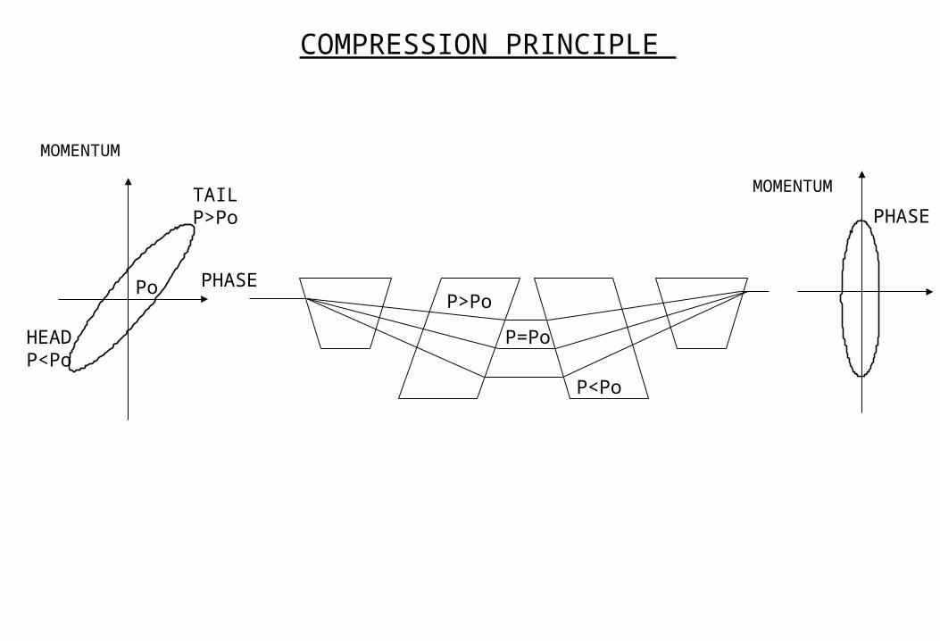
P>Po
P=Po
P<Po
COMPRESSION PRINCIPLE
Po
TAILP>Po
HEADP<Po
MOMENTUM
MOMENTUM
PHASE
PHASE

0
1
2
3
4
5
6
-100 -90 -80 -70 -60 -50 -40 -30
Homdyn simulation
Parmela simulation
Measurement
Relative phase of the superconducting cavity [Deg]
Minimum energy spread
CompressionRatio 3 mm 0.5 mm
6
Compression / Bunch length Vs. 9-cell phase
Q=8 nC, ø0=40 deg, Eo=40 MV/m, =2.1 mm, z=10.8 ps FWHM
Ib=Ip=Is= 240 A
0
5
10
15
20
25
30
35
0 2 4 6 8 10 12
x,n
y,n
Longitudinal position [m]
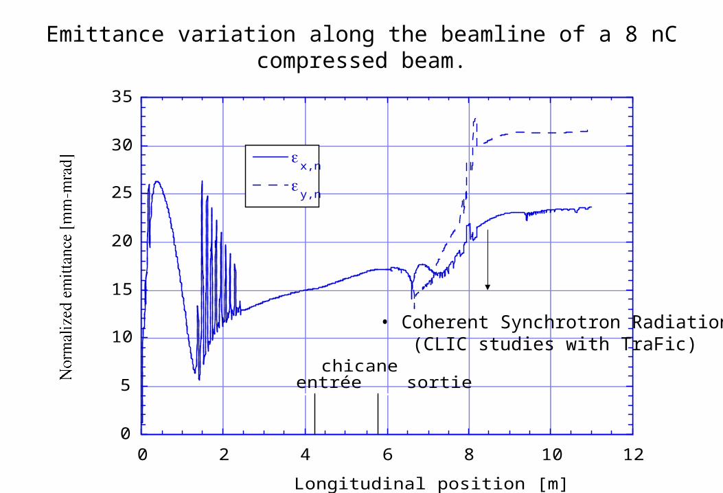
chicaneentrée sortie
Emittance variation along the beamline of a 8 nC compressed beam.
• Coherent Synchrotron Radiation (CLIC studies with TraFic)

USER EXPERIMENTS
• Electro-Optic Sampling of Transient Electric Fields, M. Fitch (thesis work). - Bunch length measurement using electro-optic detection of the electric field from the passage of a 10 nC bunch (few MV/m). • Crystal Channeling Radiation, R. Carrigan & Co. - Particle acceleration in a thin Si crystal.
• Plasma Wake Field Acceleration in Gaseous Plasma, N. Barov & Co. - Particle acceleration in a plasma: drive bunch makes a plasma wave, witness bunch is accelerated.
• Flat Beams, H. Edwards and Co. - Make emittance much smaller in one direction than in the other. Ratio 1/50 achieved to date. First accelerator to ever produce a flat beam.
• Northern Illinois University, G. Blazey and Co. - Fermilab/NICADD Photo-Injector
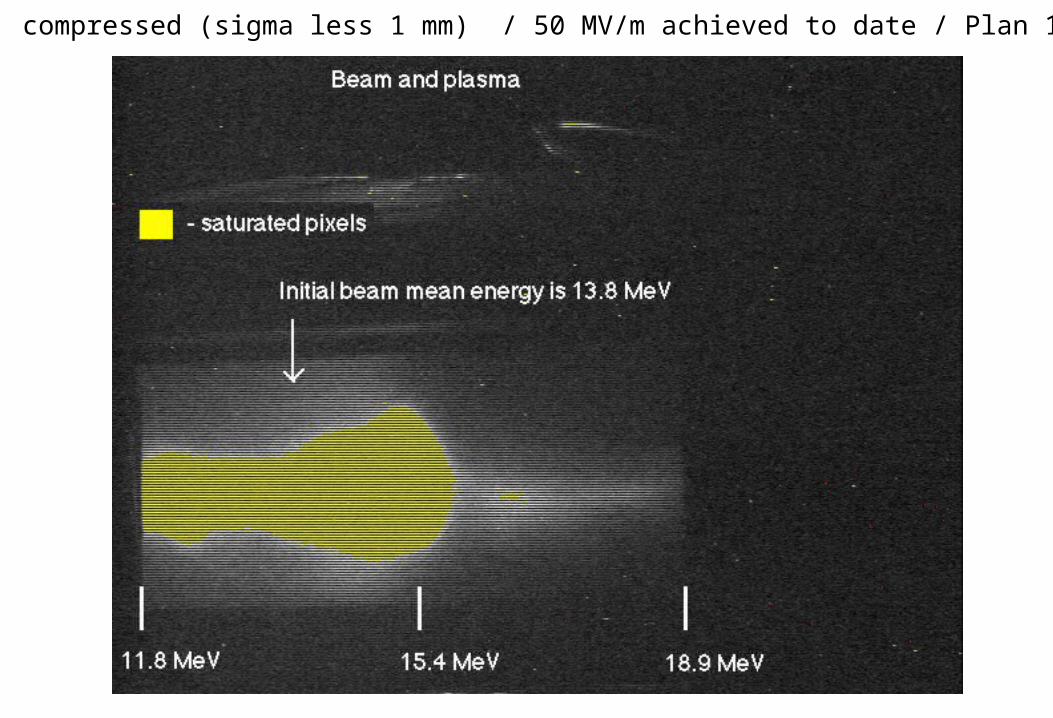
Q= 4-8 nC compressed (sigma less 1 mm) / 50 MV/m achieved to date / Plan 150 MV/m.
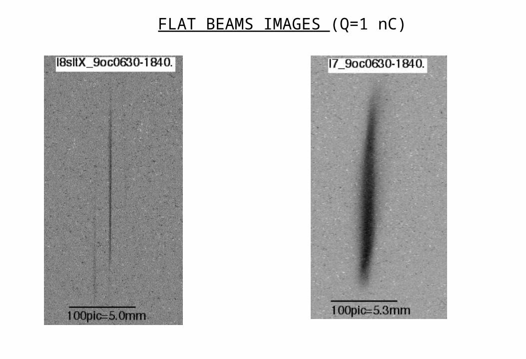
FLAT BEAMS IMAGES (Q=1 nC)
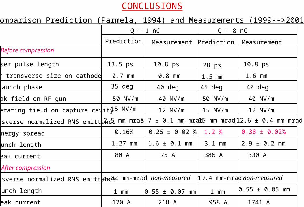
Before compression
Laser pulse length
Laser transverse size on cathode
Launch phase
Peak field on RF gun
Accelerating field on capture cavity
Transverse normalized RMS emittance
Energy spread
Bunch length
Peak current
After compression
Transverse normalized RMS emittance
Bunch length
Peak current
Q = 1 nC Q = 8 nC
Prediction Measurement Prediction Measurement
13.5 ps 10.8 ps 28 ps 10.8 ps
0.7 mm 0.8 mm 1.5 mm 1.6 mm
35 deg 40 deg 45 deg 40 deg
50 MV/m 40 MV/m 50 MV/m 40 MV/m
15 MV/m 12 MV/m 15 MV/m 12 MV/m
2.5 mm-mrad
0.16%
1.27 mm
80 A
3.02 mm-mrad
1 mm
120 A
3.7 ± 0.1 mm-mrad
0.25 ± 0.02 %
1.6 ± 0.1 mm
75 A
non-measured non-measured
0.55 ± 0.07 mm
218 A
1.2 %
3.1 mm
386 A
15 mm-mrad
19.4 mm-mrad
1 mm
958 A
0.55 ± 0.05 mm
1741 A
330 A
2.9 ± 0.2 mm
12.6 ± 0.4 mm-mrad
0.38 ± 0.02%
Comparison Prediction (Parmela, 1994) and Measurements (1999-->2001)
CONCLUSIONS
CONCLUSIONS (continued)
• The Photo-Injector designed by Fermilab meets its specifications. • Possible future studies of the photo-injector:
- Understand the dark current source. - Understand the dark current and QE “zig-zag” as a function of time for round beam and flat beam settings. - Measure emittance of a non-compressed beam using 20 ps FWHM laser pulse to see if we can decrease the emittance further. - Measure the transverse emittance of a compressed beam to study the predicted emittance increase in the deflection plan (as CERN studies).
- Pursue the user experiments.


