Download - The Global Land-Ocean Temperature Index in Relation to ... · THE GLOBAL LAND-OCEAN ... examines the statistical relationships between 10-year mov-ing averages (10-yma) of the Global

NASA/TP—2013–217485

The Global Land-Ocean Temperature Index in Relation to Sunspot Number, the Atlantic Multidecadal Oscillation Index, the Mauna Loa Atmospheric Concentration of CO2, and Anthropogenic Carbon EmissionsRobert M. WilsonMarshall Space Flight Center, Huntsville, Alabama

July 2013

National Aeronautics andSpace AdministrationIS20George C. Marshall Space Flight CenterHuntsville, Alabama 35812

The NASA STI Program…in Profile

Since its founding, NASA has been dedicated to the advancement of aeronautics and space science. The NASA Scientific and Technical Information (STI) Program Office plays a key part in helping NASA maintain this important role.

The NASA STI Program Office is operated by Langley Research Center, the lead center for NASA’s scientific and technical information. The NASA STI Program Office provides access to the NASA STI Database, the largest collection of aeronautical and space science STI in the world. The Program Office is also NASA’s institutional mechanism for disseminating the results of its research and development activities. These results are published by NASA in the NASA STI Report Series, which includes the following report types:

• TECHNICAL PUBLICATION. Reports of completed research or a major significant phase of research that present the results of NASA programs and include extensive data or theoretical analysis. Includes compilations of significant scientific and technical data and information deemed to be of continuing reference value. NASA’s counterpart of peer-reviewed formal professional papers but has less stringent limitations on manuscript length and extent of graphic presentations.

• TECHNICAL MEMORANDUM. Scientific and technical findings that are preliminary or of specialized interest, e.g., quick release reports, working papers, and bibliographies that contain minimal annotation. Does not contain extensive analysis.

• CONTRACTOR REPORT. Scientific and technical findings by NASA-sponsored contractors and grantees.

• CONFERENCE PUBLICATION. Collected papers from scientific and technical conferences, symposia, seminars, or other meetings sponsored or cosponsored by NASA.

• SPECIAL PUBLICATION. Scientific, technical, or historical information from NASA programs, projects, and mission, often concerned with subjects having substantial public interest.

• TECHNICAL TRANSLATION. English-language translations of foreign

scientific and technical material pertinent to NASA’s mission.

Specialized services that complement the STI Program Office’s diverse offerings include creating custom thesauri, building customized databases, organizing and publishing research results…even providing videos.

For more information about the NASA STI Program Office, see the following:

• Access the NASA STI program home page at <http://www.sti.nasa.gov>

• E-mail your question via the Internet to <[email protected]>

• Fax your question to the NASA STI Help Desk at 443 –757–5803

• Phone the NASA STI Help Desk at 443 –757–5802

• Write to: NASA STI Help Desk NASA Center for AeroSpace Information 7115 Standard Drive Hanover, MD 21076–1320

i

NASA/TP—2013–217485


July 2013

National Aeronautics andSpace Administration

Marshall Space Flight Center • Huntsville, Alabama 35812

ii

Available from:

NASA Center for AeroSpace Information7115 Standard Drive

Hanover, MD 21076 –1320443 –757– 5802

This report is also available in electronic form at<https://www2.sti.nasa.gov/login/wt/>

iii

TABLE OF CONTENTS

1. INTRODUCTION ............................................................................................................. 1

2. RESULTS ........................................................................................................................... 2

3. DISCUSSION AND CONCLUSION ................................................................................ 15

REFERENCES ....................................................................................................................... 17

iv

LIST OF FIGURES

1. Variation of annual (thin line) and 10-yma (thick line) values of (a) GLOTI, (b) SSN, (c) AMO, and (d) MLCO2 for the common interval 1959–2011 .................... 3

2. Scatter plots of the 10-yma values of GLOTI versus (a) SSN, (b) AMO, and (c) MLCO2 for the interval 1964–2006 ........................................................................ 4

3. Scatter plots of the 10-yma values of GLOTI versus selected BV fits for GLOTI, including (a) BV1, based on SSN and AMO, (b) BV2, based on SSN and MLCO2, and (c) BV3, based on AMO and MLCO2 .................................................................. 6

4. Scatter plot of the 10-yma values of GLOTI versus a TV fit for GLOTI (TV1), based on SSN, AMO, and MLCO2 ............................................................................. 7

5. Scatter plots of the 10-yma values of MLCO2 versus (a) GLOTI and (b) BV4, the BV fit based on GLOTI and AMO ........................................................................ 8

6. Estimated and observed 10-yma values of MLCO2 for the interval 1885–2006, based on the inferred regressions shown in figure 5 ...................................................... 9

7. Comparison of the estimated (based on BV4) and observed 10-yma values of MLCO2 for the interval 1885–2006 with exponentials based on year t .................... 10

8. The (a) first and (b) second differences of the 10-yma values of MLCO2 for the interval 1964–2006 ....................................................................................................... 12

9. Annual and 10-yma values of the TCE estimates for the interval 1959–2009 (taken from Boden, Marland, and Andres, 2012) ......................................................... 13

10. Scatter plot of the 10-yma values of MLCO2 versus TCE and TCE versus MLCO2 ............................................................................................................ 14

v

LIST OF ABBREVIATIONS, ACRONYMS, AND SYMBOLS

10-yma 10-year moving average

AMO Atlantic Multidecadal Oscillation

BV bivariate

CO2 carbon dioxide

GLOTI Global Land-Ocean Temperature Index

MLCO2 Mauna Loa CO2

SSN sunspot number

SST sea-surface temperature

TCE total carbon emissions

THC thermohaline circulation

TP Technical Publication

TV trivariate

vi

NOMENCLATURE

cl confidence level

na number above median

nb number below median

nra number of runs above median

Ry12 sample coefficient of multiple determination

r coefficient of correlation

r2 coefficient of determination

Sy12 sample standard error of estimate for multiple determination

sd standard deviation

se standard error of estimate

t time

x independent variable in regression equation

y dependent variable in regression equation

z normal deviate of the sample

1

TECHNICAL PUBLICATION

THE GLOBAL LAND-OCEAN TEMPERATURE INDEX IN RELATION TO SUNSPOT NUMBER, THE ATLANTIC MULTIDECADAL OSCILLATION INDEX, THE MAUNA LOA

ATMOSPHERIC CONCENTRATION OF CO2, AND ANTHROPOGENIC CARBON EMISSIONS

1. INTRODUCTION

Global warming/climate change has been a subject of scientific interest since the early 19th century.1–7 In particular, increases in the atmospheric concentration of carbon dioxide (CO2) have long been thought to account for Earth’s increased warming,8–16 although the lack of a dependable set of observational data was apparent as late as the mid 1950s.17–20 However, beginning in the late 1950s, being associated with the International Geophysical Year, the opportunity arose to begin accu-rate continuous monitoring of the Earth’s atmospheric concentration of CO2.21–26 Consequently, it is now well established that the atmospheric concentration of CO2, while varying seasonally within any particular year, has steadily increased over time.27–29 Associated with this rising trend in the atmospheric concentration of CO2 is a rising trend in the surface-air and sea-surface temperatures (SSTs).30–36

This Technical Publication (TP) examines the statistical relationships between 10-year mov-ing averages (10-yma) of the Global Land-Ocean Temperature Index (GLOTI), sunspot number (SSN), the Atlantic Multidecadal Oscillation (AMO) index, and the Mauna Loa CO2 (MLCO2) index for the common interval 1964–2006, where the 10-yma values are used to indicate trends in the data. Scatter plots using the 10-yma values between GLOTI and each of the other parameters are determined, both as single-variate and multivariate fits. Scatter plots are also determined for MLCO2 using single-variate and bivariate (BV) fits, based on the GLOTI alone and the GLOTI in combina-tion with the AMO index. On the basis of the inferred preferential fits for MLCO2, estimates for MLCO2 are determined for the interval 1885–1964, thereby yielding an estimate of the preindustrial level of atmospheric concentration of CO2. Lastly, 10-yma values of MLCO2 are compared against 10-yma estimates of the total carbon emissions (TCE)37 to determine the likelihood that manmade sources of carbon emissions are indeed responsible for the recent warming now being experienced. (Parametric values used in this TP are those available prior to the end of 2012.)

2

2. RESULTS

Figure 1 displays the variation of the annual (thin line) and 10-yma (thick line) values of (a) GLOTI, (b) SSN, (c) AMO, and (d) MLCO2 for the common interval 1959–2011. Individual sunspot cycles are identified in subpanel (b). Inspection of figure 1 suggests that during the common interval 1959–2011, the GLOTI, AMO, and MLCO2 are all trending upwards, while SSN is trend-ing downwards. Furthermore, because the 10-yma value of MLCO2 remains above its annual (same year) average during this common interval, it is apparent that the atmospheric concentration of CO2 as measured at Mauna Loa, Hawaii, is presently increasing at an accelerated rate, as placement of a straight-edge along the curve clearly shows.

The GLOTI is a measure of the global land-ocean temperature relative to the base period of 1951–1980, where the data are taken from the Global Historical Climate Network, version 3, using elimination of outliers and homogeneity adjustment. The data, as used in figure 1(a), are the January–December averages, available online at <http://data.giss.nasa.gov/gistemp>.33,38

The SSN provides a measure of the strength of solar activity associated with the vari-ation of solar irradiance over the solar cycle.39–42 Annual values of SSN are available online at <ftp://ftp.ngdc.noaa.gov/STP/SOLAR_DATA/SUNSPOT_NUMBERS/INTERNATIONAL>.

The AMO is a temperature oscillation in the detrended SST of the North Atlantic Ocean (0–70° N.) having a period of about 65–70 years that fluctuates between warm (positive) and cool (negative) phases.43,44 The SST pattern has been suggested to be linked to variations in the strength of the Atlantic thermohaline circulation (THC), a density-driven, global circulation pattern that involves the movement of warm equatorial surface waters to higher latitudes and the subsequent cooling and sinking of these waters in the deep ocean.45 In particular, the warm phase of the AMO represents intervals of faster THC, while the cold phase represents intervals of slower THC. From figure 1(c), one surmises that the AMO was reflective of the cool phase between about 1964 and 1994, but now is in the midst of a warm phase (since 1995) that began its rise to more positive values about 1975 (based on 10-yma values). The warm phase is expected to continue for at least another decade or more. Monthly values of the AMO index are available online at <http://www.esrl.noaa.gov/ psd/data/correlation/amon.us.long.data>.

The MLCO2 is a measure of the atmospheric concentration of CO2 as measured at the Mauna Loa Observatory on the Big Island of Hawaii, located on the northern slope of the volcano Mauna Loa at an elevation of 3,400 m above sea level and 800 m below its summit at 19.5° N. and 155.6° W.24,46 Annual averages of the MLCO2 measurements, expressed in ppm, are available online for the interval 1959–2011 at <ftp://ftp.cmdl.noaa.gov/ccg/co2/trends/co2_annmean_mlo.txt>.

3

SSN

GLOT

IML

CO2

AMO

0.5

0

–0.5

400

350

300

1

0.5

0

–0.5

Global Land-Ocean Temperature Index1959–2011

Sunspot Number1959–2011

Atlantic Multidecadal Oscillation Index1959–2011

Mauna Loa CO2 Index1959–2011

200

150

100

50

0

1960 1970

19 20 21 22 23 24

1980 1990 2000 2010Year

F1

(b)

(a)

(c)

(d)

Figure 1. Variation of annual (thin line) and 10-yma (thick line) values of (a) GLOTI, (b) SSN, (c) AMO, and (d) MLCO2 for the common interval 1959–2011.

4

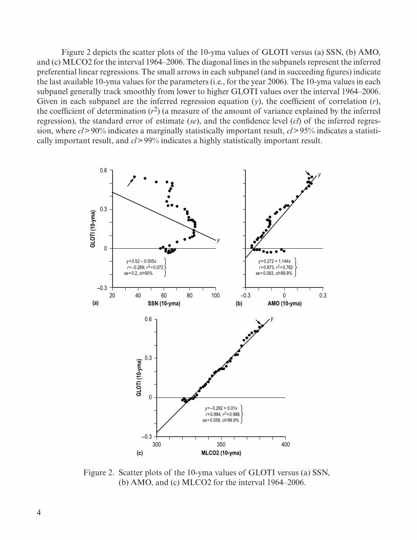
Figure 2 depicts the scatter plots of the 10-yma values of GLOTI versus (a) SSN, (b) AMO, and (c) MLCO2 for the interval 1964–2006. The diagonal lines in the subpanels represent the inferred preferential linear regressions. The small arrows in each subpanel (and in succeeding figures) indicate the last available 10-yma values for the parameters (i.e., for the year 2006). The 10-yma values in each subpanel generally track smoothly from lower to higher GLOTI values over the interval 1964–2006. Given in each subpanel are the inferred regression equation (y), the coefficient of correlation (r), the coefficient of determination (r2) (a measure of the amount of variance explained by the inferred regression), the standard error of estimate (se), and the confidence level (cl) of the inferred regres-sion, where cl > 90% indicates a marginally statistically important result, cl > 95% indicates a statisti-cally important result, and cl > 99% indicates a highly statistically important result.

GLOT

I (10

-ym

a)

0.6

0.3

0

–0.3

GLOT

I (10

-ym

a)

0.6

0.3

0

–0.3

(a)20 40 60 80 100

SSN (10-yma)

y

y=0.52 – 0.005xr=–0.269, r2=0.072

se=0.2, cl>90%

(b)–0.3 0 0.3

AMO (10-yma)

y=0.272 + 1.144xr=0.873, r2=0.762

se=0.093, cl>99.9%

y

y

(c)300 350 400

F2

MLCO2 (10-yma)

y=–3.282 + 0.01xr=0.994, r2=0.988

se=0.058, cl>99.9%

Figure 2. Scatter plots of the 10-yma values of GLOTI versus (a) SSN, (b) AMO, and (c) MLCO2 for the interval 1964–2006.

5

For GLOTI versus SSN, the inferred regression based on the limited time interval 1964–2006 is one found to be only of marginal statistical importance, having cl > 90%, se = 0.2 °C, and r2 = 0.072, meaning that the inferred regression explains only about 7% of the variance in the 10-yma values of GLOTI during the interval 1964–2006. Also, the inferred regression is found to be one that varies inversely (r = –0.27) rather than directly, in contrast to that found when using the much longer inter-val 1885–2006, one that clearly shows an upward-trending SSN.47

For GLOTI versus AMO, the inferred regression (r = 0.87) is one that is highly statistically important, having cl > 99.9%, se = 0.09 °C, and r2 = 0.762, meaning that the inferred regression explains about 76% of the variance in the 10-yma values of GLOTI. Current values of AMO and GLOTI are positive, indicative of the warm phase and the occurrence of a warm anomaly, respec-tively. The implication then is that the continuing warm phase as indicated by the AMO suggests a continuing positive (warm) global land-ocean temperature anomaly for the near term foreseeable future.

For GLOTI versus MLCO2, the inferred regression (r = 0.99) is the strongest of all the inferred regressions, having cl > 99.9%, se = 0.06 °C, and r2 = 0.988, meaning that the inferred regres-sion explains nearly 99% of the variance in the 10-yma values of GLOTI for the interval 1964–2006. The implication then is that the continuing unabated increase in the atmospheric concentration of CO2 as measured at Mauna Loa strongly suggests a continuing increase in the positive (warm) global land-ocean temperature for the long term foreseeable future.

6

Figure 3 shows the scatter plots of the 10-yma values of GLOTI versus selected BV fits for GLOTI, including (a) BV1, based on SSN and AMO, (b) BV2, based on SSN and MLCO2, and (c) BV3, based on AMO and MLCO2. The BV fit BV1, having Ry12 = 0.895 and Sy12 = 0.086 °C, represents a slight improvement over using AMO alone, while the BV fit BV2, having Ry12 = 0.994 and Sy12 = 0.021 °C, and especially BV fit BV3, having Ry12 = 0.999 and Sy12 = 0.01 °C, represent sig-nificant improvements over using MLCO2 alone (by virtue of their inferred reduced standard error of estimates). (In figure 3, subscripts 1 and 2 refer to parameters 1 and 2, where 1 is SSN and 2 is AMO in BV1; SSN and MLCO2 in BV2; and AMO and MLCO2 in BV3.)

GLOT

I (10

-ym

a)

0.6

0.3

0

–0.3

(a)

GLOT

I (10

-ym

a)

0.6

0.3

0

–0.3

(c)

–0.3 0 0.3 0.6GLOTI (SSN, AMO) (10-yma)=BV1

BV1=0.004 + 0.004SSN + 1.296AMORy12=0.895, Sy12=0.086

(b)–0.3 0 0.3 0.6

GLOTI (SSN, MLCO2) (10-yma)=BV2

BV2 = –3.21747 – 0.00054SSN + 0.0096MLCO2Ry12=0.99432, Sy12=0.0205

–0.3 0 0.3 0.6

F3

GLOTI (AMO, MLCO2) (10-yma)=BV3

BV3=–2.774421 + 0.224552AMO + 0.008615MLCO2Ry12=0.998623, Sy12=0.010105

Figure 3. Scatter plots of the 10-yma values of GLOTI versus selected BV fits for GLOTI, including (a) BV1, based on SSN and AMO, (b) BV2, based on SSN and MLCO2, and (c) BV3, based on AMO and MLCO2.

7

Figure 4 displays the scatter plot of the 10-yma values of GLOTI versus a trivariate (TV) fit for GLOTI (TV1), based on SSN, AMO, and MLCO2. Essentially, the TV1 fit is insignificantly dif-ferent from that of the BV3 fit (i.e., the r and se are essentially the same for both fits).

GLOT

I (10-

yma)

0.6

0.3

0

–0.3–0.3 0 0.3 0.6

GLOTI (SSN, AMO, MLCO2) (10-yma)=TV1

f4

TV1=–0.032296 + 0.000441SSN + 1.00606BV3Ry12=0.998689, Sy12=0.009859

Figure 4. Scatter plot of the 10-yma values of GLOTI versus a TV fit for GLOTI (TV1), based on SSN, AMO, and MLCO2.

8

Figure 5 depicts the scatter plots of the 10-yma values of MLCO2 versus (a) GLOTI and (b) BV4, the BV fit based on both GLOTI and AMO. Of the two fits, the one between MLCO2 and GLOTI alone is the stronger, having r = 0.994 and se = 2 ppm, as compared to Ry12 = 0.992 and Sy12 = 2.4 ppm for BV4. The diagonal line in figure 5(a) is the inferred preferential linear regression line for MLCO2 versus GLOTI. The regression equations and other statistical parameters are identi-fied in the subpanels.

MLCO

2 (10

-ym

a)

400

350

300

(a)–0.3 0 0.3

y

0.6GLOTI (10-yma) (b)

300 350 400MLCO2 (GLOTI, AMO)=BV4

F5

y=327.208 + 98.404x

se=2.047, cl>99.9% r=0.994, r2=0.988

BV4=322.309 + 115.027GLOTI – 25.038AMORy12=0.992, Sy12=2.422

Figure 5. Scatter plots of the 10-yma values of MLCO2 versus (a) GLOTI and (b) BV4, the BV fit based on GLOTI and AMO.

9

Figure 6 shows the estimated and observed 10-yma values of MLCO2 for the interval 1885–2006 based on the inferred regressions shown in figure 5. Thus, presuming the validity of the inferred regressions, one finds that, while both fits essentially mimic the observed 10-yma values of MLCO2 (the filled circles) for the interval 1970–2006, slight differences are apparent in the values prior to 1970. In particular, BV4 (the thick line) suggests slightly lower estimated values (by about 10 ppm) for the 10-yma values of MLCO2 during the interval 1885–1964, as compared to using the linear fit based on GLOTI alone. Both extrapolations suggest temporary slight increases in atmospheric concentration of CO2 near 1900 and the early 1940s, each increase lasting about 20 years in length. Values since about 1975 have been the highest on record and continue to increase with the passage of time.

MLCO

2 (10

-ym

a)

250

300

350

400

1880 1900 1920 1940 1960 1980 2000 2020Year

F6

y=327.208 + 98.404GLOTI

BV4=322.309 + 115.027GLOTI – 25.038AMORy12= 0.992, Sy12=2.422

MLCO2 (Observed)

r=0.994, se =2.047

Figure 6. Estimated and observed 10-yma values of MLCO2 for the interval 1885–2006, based on the inferred regressions shown in figure 5.

10

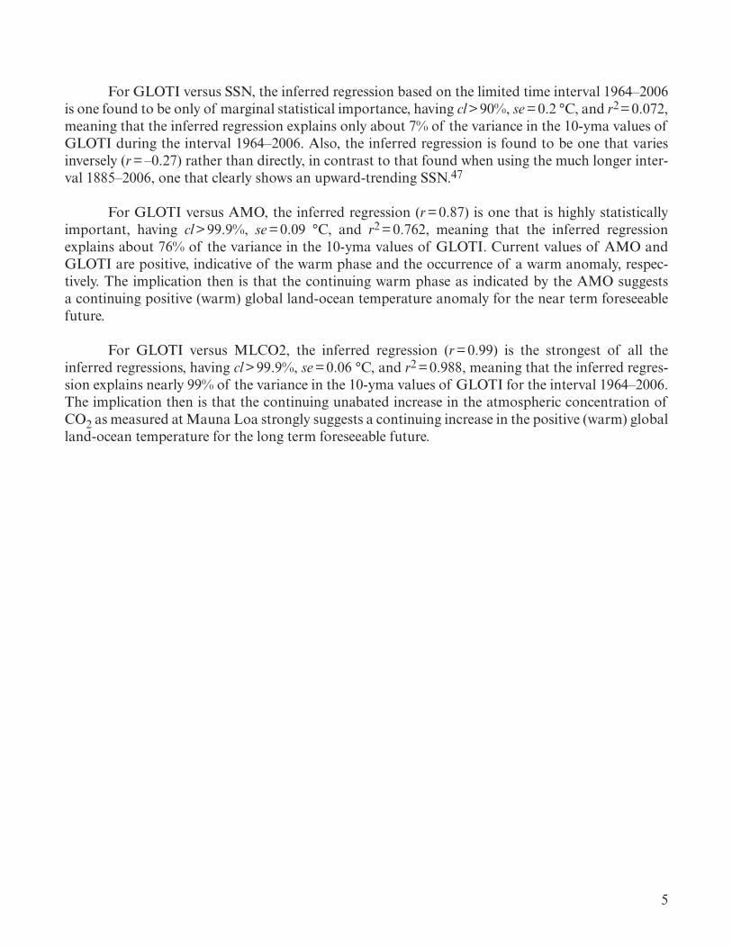
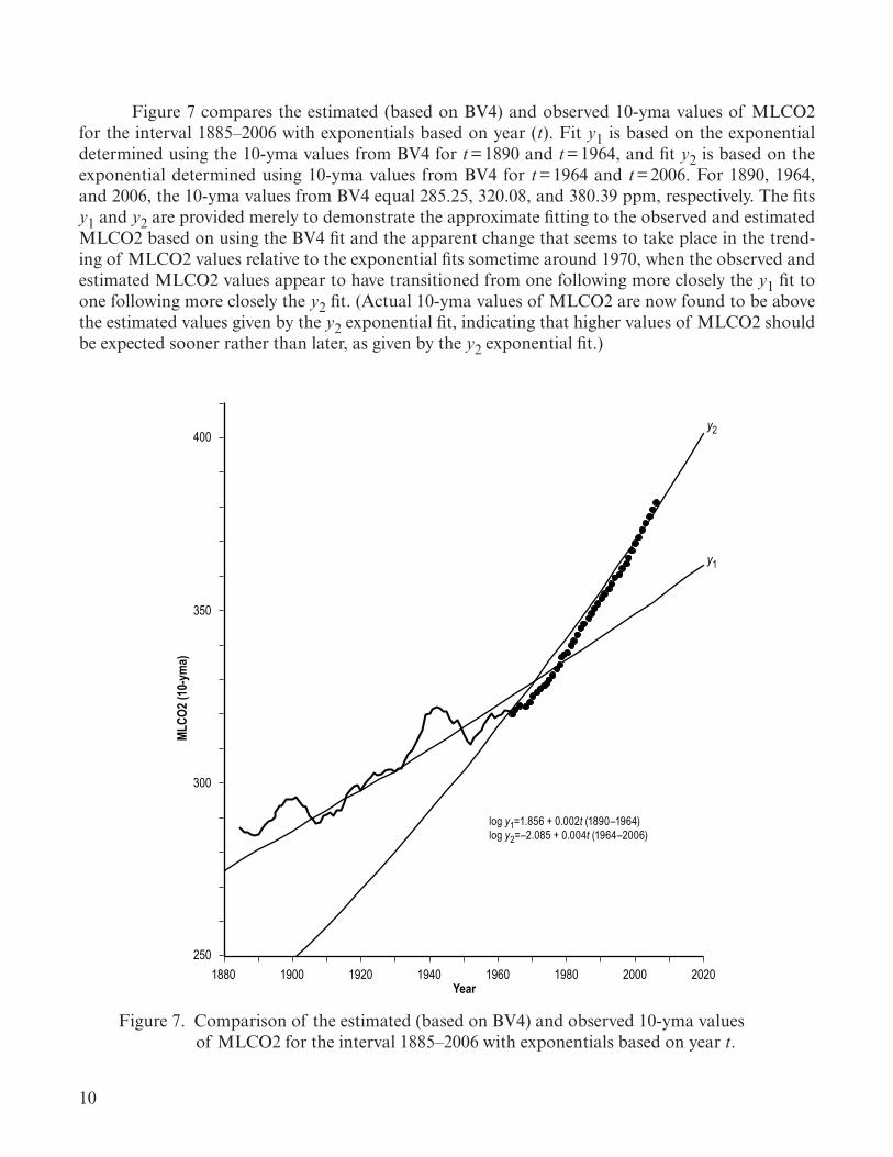
Figure 7 compares the estimated (based on BV4) and observed 10-yma values of MLCO2 for the interval 1885–2006 with exponentials based on year (t). Fit y1 is based on the exponential determined using the 10-yma values from BV4 for t = 1890 and t = 1964, and fit y2 is based on the exponential determined using 10-yma values from BV4 for t = 1964 and t = 2006. For 1890, 1964, and 2006, the 10-yma values from BV4 equal 285.25, 320.08, and 380.39 ppm, respectively. The fits y1 and y2 are provided merely to demonstrate the approximate fitting to the observed and estimated MLCO2 based on using the BV4 fit and the apparent change that seems to take place in the trend-ing of MLCO2 values relative to the exponential fits sometime around 1970, when the observed and estimated MLCO2 values appear to have transitioned from one following more closely the y1 fit to one following more closely the y2 fit. (Actual 10-yma values of MLCO2 are now found to be above the estimated values given by the y2 exponential fit, indicating that higher values of MLCO2 should be expected sooner rather than later, as given by the y2 exponential fit.)

MLCO

2 (10

-ym

a)

250

300

y2

y1

400

350

1880 1900 1920 1940 1960 1980 2000 2020Year

f7

log y1= 1.856 + 0.002t (1890–1964) log y2=–2.085 + 0.004t (1964–2006)

Figure 7. Comparison of the estimated (based on BV4) and observed 10-yma values of MLCO2 for the interval 1885–2006 with exponentials based on year t.

11

The expected 10-yma value of MLCO2 about 1880 is of interest because it is representative of the preindustrial level of the atmospheric concentration of CO2. Now, the record of GLOTI yearly values begins in 1880, having a value of –0.32 °C. Consequently, the first available 10-yma value of GLOTI occurs in 1885. However, the record of AMO yearly values begins in 1856, so that the 10-yma value of AMO is known for 1880 (=0.075 °C). For the interval 1885–2006, the residual (i.e., the difference between the yearly value and the corresponding 10-yma value) for GLOTI is about ± 0.1 °C, a range that captures about 80% of the residuals.47 Hence, one can estimate the 10-yma value for GLOTI for the year 1880 to be about –0.32 ± 0.1 °C. Using this value in conjunction with the 10-yma AMO value for 1880 in BV4 allows one to estimate the 10-yma value of MLCO2 for 1880, a value computed to be about 283.6 ± 2.4 ppm, very close to that determined from polar ice cores for the preindustrial level (i.e., about 280 ± 5 ppmv; see Neftel et al.48).

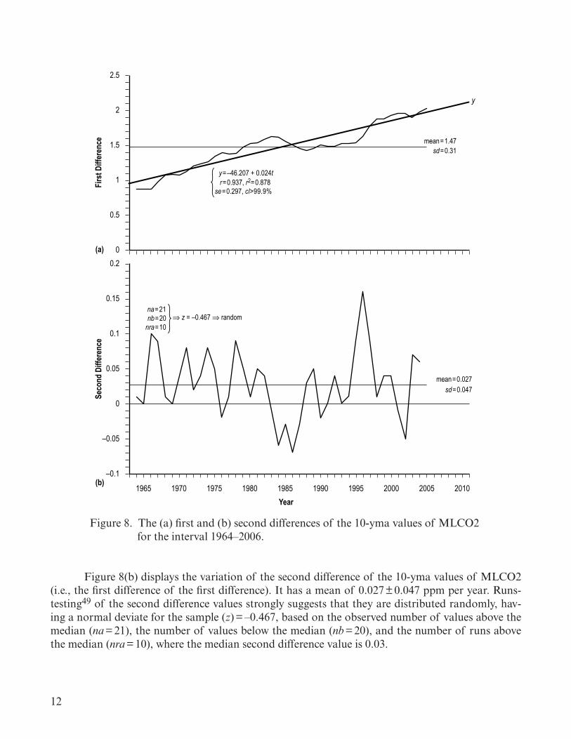
As previously noted, the atmospheric concentration of CO2 as measured at Mauna Loa appears to be not only increasing over time, but also to be increasing at an accelerated rate. Figure 8 plots the (a) first and (b) second differences of the 10-yma values of MLCO2 for the interval 1964–2006. From figure 8(a), one finds that the average 10-yma value of MLCO2 is growing at the rate of about 1.47 ± 0.31 ppm per year (i.e., the mean ± 1 standard deviation (sd) interval). However, as can be seen from figure 8(a), the average rate inadequately describes the actual year-to-year first difference values. The rate of growth in the 10-yma value of MLCO2 was always below 1.5 ppm prior to 1980 and, except for the brief intervals 1987–1989 and 1991–1992, it always has been equal to 1.5 ppm or greater after 1980, measuring 2.03 ppm in 2005 (the last available first difference value and the largest rate of growth ever measured). Overall, the first difference values are better described using the linear fit given by y = –46.207 + 0.024t, where y is the expected first difference and t is the year, rather than using the mean and sd. The linear fit is found to explain about 88% of the variance in the first difference values. For 2006, one expects the first difference to be about 1.99 ± 0.3 ppm (the ±1 se prediction interval), thereby inferring that the expected 10-yma of MLCO2 for 2007 should be about 381.6 + 1.99 ± 0.3 ppm or about 383.59 ± 0.3 ppm. Presuming the validity of the fit, one esti-mates the 10-yma value of MLCO2 for 2015 and 2026 to be ≥400 ppm and ≥425 ppm, respectively. If these values prove true, then, from figure 2(c), one expects the 10-yma value of GLOTI to measure about 0.72 ± 0.06 °C in 2015 and about 0.97 ± 0.06 °C in 2026. (It should be noted that the 10-yma of MLCO2 for 2007 is now known to measure 383.67 ppm, thus confirming the prediction above that it would measure about 383.59 ± 0.3 ppm.)

12

Firs

t Diff

eren

ceSe

cond

Diff

eren

ce

0.2

0.15

0.1

0.05

0

–0.05

–0.1

2.5

2

1.5

1

0.5

0

1965 1970 1975 1980 1985 1990 1995 2000 2005 2010Year

f8

(a)

(b)

na=21nb=20 ⇒ z = –0.467 ⇒ random

nra=10

mean=0.027

mean=1.47sd= 0.31

y=–46.207 + 0.024tr=0.937, r2=0.878

se=0.297, cl>99.9%

y

sd=0.047

Figure 8. The (a) first and (b) second differences of the 10-yma values of MLCO2 for the interval 1964–2006.

Figure 8(b) displays the variation of the second difference of the 10-yma values of MLCO2 (i.e., the first difference of the first difference). It has a mean of 0.027 ± 0.047 ppm per year. Runs-testing49 of the second difference values strongly suggests that they are distributed randomly, hav-ing a normal deviate for the sample (z) = –0.467, based on the observed number of values above the median (na = 21), the number of values below the median (nb = 20), and the number of runs above the median (nra = 10), where the median second difference value is 0.03.

13

Recently, Boden et al. reported on the yearly variation of global fossil fuel CO2 emissions.37

They noted that approximately 356 billion metric tons of carbon have been released into the atmo-sphere through the combustion of fossil fuels and cement production since 1751, with half of the fossil fuel CO2 emissions having occurred since the mid 1980s. Furthermore, they noted that liquid and solid fuels accounted for about 76.6% of the emissions in 2009, while gas fuels (e.g., natural gas) and cement production accounted for 17.9% and 4.7% of the emissions, respectively.

Figure 9 plots the annual and 10-yma values of the TCE estimates for the interval 1959–2009. For the overall interval 1964–2004, the trend in TCE has grown at the average rate of about 118 million metric tons per year, although the intervals prior to 1975 and after about 1997 have had considerably higher average rates of growth, measuring about 157 and 169 million metric tons per year, respectively. Extrapolation of the 10-yma trend line beyond 2004 using the higher rate of growth in TCE suggests that TCE will measure about 10,000 million metric tons around the year 2017 ± 2 years, and it will measure about 12,000 million metric tons around 2029 ± 2 years. (The rightmost vertical axis gives the total CO2 emission in units of million metric tons.)

Tota

l Car

bon

Emiss

ions

(in

milli

on m

etric

tons

)Total Carbon Dioxide Em

issions (in million m

etric tons)

104

9×103 33×103

22×103

11×103

8×103

7×103

6×103

5×103

4×103

3×103

2×103

1960 1965 1970 1975 1980 1985 1990 1995 2000 2005 2010Year

F9

Total Global Fossil Fuel Carbon Emissions1959–2009(Boden, Marlard, and Andres, 2012)

Figure 9. Annual and 10-yma values of the TCE estimates for the interval 1959–2009 (taken from Boden, Marland, and Andres, 2012).37

14

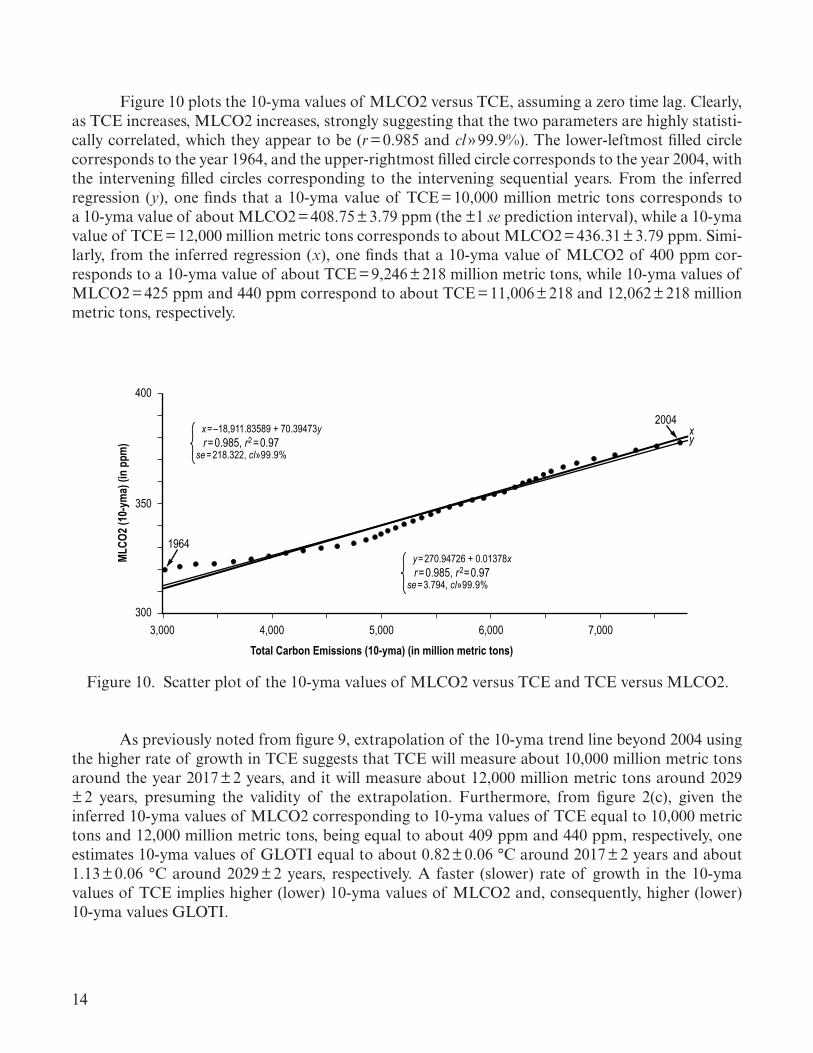
Figure 10 plots the 10-yma values of MLCO2 versus TCE, assuming a zero time lag. Clearly, as TCE increases, MLCO2 increases, strongly suggesting that the two parameters are highly statisti-cally correlated, which they appear to be (r = 0.985 and cl » 99.9%). The lower-leftmost filled circle corresponds to the year 1964, and the upper-rightmost filled circle corresponds to the year 2004, with the intervening filled circles corresponding to the intervening sequential years. From the inferred regression (y), one finds that a 10-yma value of TCE = 10,000 million metric tons corresponds to a 10-yma value of about MLCO2 = 408.75 ± 3.79 ppm (the ±1 se prediction interval), while a 10-yma value of TCE = 12,000 million metric tons corresponds to about MLCO2 = 436.31 ± 3.79 ppm. Simi-larly, from the inferred regression (x), one finds that a 10-yma value of MLCO2 of 400 ppm cor-responds to a 10-yma value of about TCE = 9,246 ± 218 million metric tons, while 10-yma values of MLCO2 = 425 ppm and 440 ppm correspond to about TCE = 11,006 ± 218 and 12,062 ± 218 million metric tons, respectively.

MLCO

2 (10

-ym

a) (i

n pp

m)

400

350

1964

3003,000 4,000 5,000 6,000 7,000

Total Carbon Emissions (10-yma) (in million metric tons)

f10

y=270.94726 + 0.01378xr=0.985, r2=0.97

se=3.794, cl»99.9%

x=–18,911.83589 + 70.39473yr=0.985, r2=0.97

se=218.322, cl»99.9%yx

2004

Figure 10. Scatter plot of the 10-yma values of MLCO2 versus TCE and TCE versus MLCO2.

As previously noted from figure 9, extrapolation of the 10-yma trend line beyond 2004 using the higher rate of growth in TCE suggests that TCE will measure about 10,000 million metric tons around the year 2017 ± 2 years, and it will measure about 12,000 million metric tons around 2029 ± 2 years, presuming the validity of the extrapolation. Furthermore, from figure 2(c), given the inferred 10-yma values of MLCO2 corresponding to 10-yma values of TCE equal to 10,000 metric tons and 12,000 million metric tons, being equal to about 409 ppm and 440 ppm, respectively, one estimates 10-yma values of GLOTI equal to about 0.82 ± 0.06 °C around 2017 ± 2 years and about 1.13 ± 0.06 °C around 2029 ± 2 years, respectively. A faster (slower) rate of growth in the 10-yma values of TCE implies higher (lower) 10-yma values of MLCO2 and, consequently, higher (lower) 10-yma values GLOTI.

15

3. DISCUSSION AND CONCLUSION

This TP of the common interval 1964–2006 has revealed a close statistical coupling between the global land-ocean temperature anomaly as described by GLOTI and both the phase of the AMO and the increasing atmospheric concentration of CO2 as measured at Mauna Loa. On the basis of 10-yma values, the GLOTI is found to be well described using the BV fit BV3 = –2.77 + 0.224552AMO + 0.008615MLCO2, having Ry12 = 0.9986 and Sy12 = 0.01 °C, where BV3 represents the 10-yma of value of the GLOTI, and the subscripts 1 and 2 refer to the 10-yma parametric values of the AMO and MLCO2 indices, respectively. Likewise, the BV fit BV4 (=322.309 + 115.027GLOTI – 25.038AMO) is found to provide a very close fit for the observed 10-yma values of MLCO2, having Ry12 = 0.992 and Sy12 = 2.42 ppm.

From an extrapolation of the BV4 fit backwards in time, prior to 1964, one finds evidence for two temporary slight increases in the atmospheric concentration of CO2, each of about 20 years dura-tion—the first about 1900, having a local peak of about 296 ± 2.4 ppm, and the second in the early 1940s, having a local peak of about 322 ± 2.4 ppm. While the interval prior to about 1970 appears to be better approximated using the exponential log y1 = 1.856 + 0.002t, where y1 is the 10-yma value of MLCO2 and t is the year, the interval after 1970 appears to be better described using the exponential y2 = –2.085 + 0.004t. However, current 10-yma values of MLCO2 now appear to be rising faster than described by the post-1970 exponential. Using the BV4 fit, one estimates the preindustrial value for the atmospheric concentration of CO2 to be about 283.6 ± 2.4 ppm, very close to that determined from polar ice cores (i.e., about 280 ± 5 ppmv).

The 10-yma value of MLCO2 measured about 382 ppm in 2006. On average, the 10-yma value of MLCO2 is found to be increasing at the approximate rate of about 1.47 ± 0.31 ppm per year. While true, the average rate of growth in the 10-yma values of MLCO2 does not appear to adequately describe the actual year-to-year increases in the 10-yma values. Instead, the rate of yearly increase is better described using the linear fit y = –46.207 + 0.024t, where y is the first difference in consecutive year-to-year 10-yma values of MLCO2 and t is the year. Hence, the 10-yma values of MLCO2 appear to be increasing at an accelerated rate, such that the 10-yma value of MLCO2 is expected to measure ≥400 ppm about the middle-to-latter half of the present decade and ≥425 ppm about the middle-to-latter half of the following decade. Likewise, because of the inferred close asso-ciation between the 10-yma values of GLOTI and MLCO2, one expects 10-yma values of GLOTI to continue to increase over time, measuring about 0.72 ± 0.06 °C and 0.97 ± 0.06 °C, respectively, when 10-yma values of MLCO2 measure ≥400 ppm and ≥425 ppm.

The rise in 10-yma values of MLCO2 appears to be directly linked to the increase in the 10-yma values of the TCE as deduced from the yearly values of global fossil fuel CO2 emissions determined by Boden et al.37 In particular, the 10-yma values of MLCO2 are found to increase in step with increases in the 10-yma values of TCE, with the inferred correlation having r = 0.985 and cl » 99.9%. From the inferred regression between the 10-yma values of MLCO2 and TCE, one finds

16

that a 10-yma value of TCE equal to about 10,000 million metric tons suggests a 10-yma value of MLCO2 ≥400 ppm and GLOTI ≥0.76 °C, while a 10-yma value of TCE equal to about 12,000 mil-lion metric tons suggests a 10-yma value of MLCO2 ≥440 ppm and GLOTI ≥1.07 °C.

17

REFERENCES

1. Mitchell, J.F.B.: “The ‘Greenhouse’ effect and climate change,” Rev. Geophys., Vol. 27, No. 1, pp. 115–139, doi:10.1029/RG027i001p00115, February 1989.

2. Jones, M.D.H.; and Henderson-Sellers, A.: “History of the greenhouse effect,” Prog. Phys. Geog., Vol. 14, No. 1, pp. 1–18, doi:10.1177/030913339001400101, March 1990.

3. Rodhe, H.; Charlson, R.; and Crawford, E.: “Svante Arrhenius and the Greenhouse Effect,” Ambio, Vol. 26, No. 1, pp. 2–5, February 1997.

4. Manabe, S.: “Early Development in the Study of Greenhouse Warming: The Emergence of Cli-mate Models,” Ambio, Vol. 26, No. 1, pp. 47–51, February 1997.

5. Solomon, S.D.; Qin, D.; Manning, M.; et al. (eds.): Climate Change 2007: The Physical Science Basis, Cambridge University Press, Cambridge, UK, 996 pp., 2007.

6. Gray, L.J.; Beer, J.; Geller, M.; et al.: “Solar influences on climate,” Rev. Geophys., Vol. 48, No. 4, 53 pp., doi:10.1029/2009RG000282, December 2010.

7. Archer, D.; and Pierrehumbert, R. (eds.): The Warming Papers: The Scientific Foundation for the Climate Change Forecast, Wiley-Blackwell, Oxford, UK, 432 pp., 2011.

8. Tyndall, J.: “On the Absorption and Radiation of Heat by Gases and Vapours, and on the Physi-cal Connexion of Radiation, Absorption, and Conduction,” Philos. T. R. Soc. Lond., Vol. 151, pp. 1–36, 1861.

9. Chamberlin, T.C.: “An Attempt to Frame a Working Hypothesis of the Cause of Glacial Peri-ods on an Atmospheric Basis,” J. Geol., Vol. 7, No. 6, pp. 545–584, 1899.

10. Arrhenius, S.: “On the Influence of Carbonic Acid in the Air upon the Temperature of the Ground,” Philos. Mag., Vol. 4, No. 251, pp. 237–276, April 1896.

11. Arrhenius, S.: Lehrbuch der kosmischen Physik 2, Verlag von S. Hirzel, Leipzig, Germany, 1903.

12. Callendar, G.S.: “The artificial production of carbon dioxide and its influence on temperature,” Q. J. Roy. Meteor. Soc., Vol. 64, No. 275, pp. 223–240, doi:10.1002/qj.49706427503, April 1938.

13. Callendar, G.S.: “Variations of the amount of carbon dioxide in different air currents,” Q. J. Roy. Meteor. Soc., Vol. 66, No. 287, pp. 395–400, doi:10.1002/qj.49706628705, October 1940.

18

14. Callendar, G.S.: “Can carbon dioxide influence climate?” Weather, Vol. 4, No. 10, pp. 310–314, doi:10.1002/j.1477-8696.1949.tb00952.x, October 1949.

15. Callendar, G.S.: “On the Amount of Carbon Dioxide in the Atmosphere,” Tellus, Vol. 10, No. 2, pp. 243–248, doi:10.1111/j.2153-3490.1958.tb02009.x, May 1958.

16. Callendar, G.S.: “Temperature fluctuations and trends over the earth,” Q. J. Roy. Meteor. Soc., Vol. 87, No. 373, pp. 435–437, doi:10.1002/qj.49708737316, July 1961.

17. Slocum, G.: “Has the amount of carbon dioxide in the atmosphere changed significantly since the beginning of the twentieth century?” Mon. Weather Rev., Vol. 83, No. 10, pp. 225–231, October 1955.

18. Fonselius, S.; Koroleff, F.; and Wärme, K.-E.: “Carbon Dioxide Variations in the Atmosphere,” Tellus, Vol. 8, No. 2, pp. 176–183, doi:10.1111/j.2153-3490.1956.tb01208.x, May 1956.

19. Revelle, R.; and Suess, H.E.: “Carbon Dioxide Exchange Between Atmosphere and Ocean and the Question of an Increase of Atmospheric CO2 during the Past Decades,” Tellus, Vol. 9, No. 1, pp. 18–27, doi:10.1111/j.2153-3490.1957.tb01849.x, February 1957.

20. Bray, J.R.: “An Analysis of the Possible Recent Change in Atmospheric Carbon Dioxide Concentration,” Tellus, Vol. 11, No. 2, pp. 220–230, doi:10.1111/j.2153-3490.1959.tb00023.x, May 1959.

21. Bolin, B.; and Eriksson, E.: “Changes in the Carbon Dioxide Content of the Atmosphere and Sea due to Fossil Fuel Combustion,” in The Atmosphere and Sea in Motion, The Rockefeller Institute Press, New York, NY, pp. 130–142, 1959.

22. Keeling, C.D.: “The Concentration and Isotropic Abundances of Carbon Dioxide in the Atmo-sphere,” Tellus, Vol. 12, No. 2, pp. 200–203, doi:10.1111/j.2153-3490.1960.tb01300.x, May 1960.

23. Bolin, B.; and Keeling, C.D.: “Large-scale atmospheric mixing as deduced from seasonal and meridional variations of carbon dioxide,” J. Geophys. Res., Vol. 68, No. 13, pp. 3899–3920, doi:10.1029/JZ068i013p03899, July 1963.

24. Pales, J.C.; and Keeling, C.D.: “The concentration of atmospheric carbon dioxide in Hawaii,” J. Geophys. Res., Vol. 70, No. 24, pp. 6053–6076, doi:10.1029/JZ070i024p06053, December 1965.

25. Brown, C.W.; and Keeling, C.D.: “The concentration of atmospheric carbon dioxide in Antarc-tica,” J. Geophys. Res., Vol. 70, No. 24, pp. 6077–6085, doi:10.1029/JZ070i024p06077, December 1965.

26. Bolin, B.; and Bischof, W.: “Variations of the carbon dioxide content of the atmosphere in the northern hemisphere,” Tellus, Vol. 22, No. 4, pp. 431–442, doi:10.1111/j.2153-3490.1970.tb00508.x, August 1970.

19

27. Keeling, C.D.; Bacastow, R.B.; Bainbridge, A.E., et al.: “Atmospheric carbon diox-ide variations at Mauna Loa Observatory, Hawaii,” Tellus, Vol. 28, No. 6, pp. 538–551, doi:10.1111/j.2153-3490.1976.tb00701.x, December 1976.

28. Bacastow, R.B.; Keeling, C.D.; and Whorf, T.P.: “Seasonal amplitude increase in atmospheric CO2 concentration at Mauna Loa, Hawaii, 1959–1982,” J. Geophys. Res., Vol. 90, No. D6, pp. 10,529–10,540, doi:10.1029/JD090iD06p10529, October 1985.

29. Thoning, K.W.; Tans, P.P.; and Komhyr, W.D.: “Atmospheric carbon dioxide at Mauna Loa Observatory 2. Analysis of the NOAA GMCC data, 1974–1985,” J. Geophys. Res., Vol. 94, No. D6, pp. 8549–8565, doi:10.1029/JD094iD06p08549, June 1989.

30. Paltridge, G.; and Woodruff, S.: “Changes in Global Surface Temperature from 1880 to 1977 Derived From Historical Records of Sea Surface Temperature,” Mon. Weather Rev., Vol. 109, No. 12, pp. 2427–2434, December 1981.

31. Wigley, T.M.L.; and Raper, S.C.B.: “Natural variability of the climate system and detection of the greenhouse effect,” Nature, Vol. 344, pp. 324–327, doi:10.1038/344324a0, March 1990.

32. Cline, W.R.: “Scientific Basis for the Greenhouse Effect,” Econ. J., Vol. 101, No. 407, pp. 904–919, July 1991.

33. Hansen, J.R.; Sato, M.; Ruedy, R.; et al.: “Global temperature change,” P. Natl. Acad. Sci. USA., Vol. 103, No. 39, pp. 14,288–14,293, doi:10.1073/pnas.0606291103, September 2006.

34. Hansen, J.; Ruedy, R.; Sato, M.; and Lo, K.: “Global surface temperature change,” Rev. Geo-phys., Vol. 48, No. 4, 29 pp., doi:10.1029/2010RG000345, December 2010.

35. Beck, E.-G.: “180 years of atmospheric CO2 gas analysis by chemical methods,” Energy & Envi-ronment, Vol. 18, No. 2, pp. 259–282, 2007.

36. Wilson, R.M.: “Solar Cycle and Anthropogenic Forcing of Surface-Air Temperature at Armagh Observatory, Northern Ireland,” NASA/TP—2010–216375, Marshall Space Flight Center, AL, 28 pp., March 2010.

37. Boden, T.A.; Marland, G.; and Andres, R.J.: “Global, Regional, and National Fossil-Fuel CO2 Emissions,” 2012, <http://cdiac.ornl.gov/trends/emis/overview_2009.html>.

38. Smith, E.M.: “Summary report on v1 vs v3 GHCN,” June 20, 2012, <http://chiefio.wordpress.com/2012/06/20/summary-report-on-v1-vs-v3-ghcn/>.

39. Willson, R.C.; and Hudson, H.S.: “The Sun’s luminosity over a complete solar cycle,” Nature, Vol. 351, No. 6321, pp. 42– 44, doi:10.1038/351042a0, May 1991.

40. Willson, R.C.: “Total Solar Irradiance Trend During Solar Cycles 21 and 22,” Science, Vol. 277, No. 5334, pp. 1963–1965, doi:10.1126/science.277.5334.1963, September 1997.

20

41. Willson, R.C.; and Mordvinov, A.V.: “Secular total solar irradiance trend during solar cycles 21–23,” Geophys. Res. Lett., Vol. 30, No. 5, pp. 21–23, doi:10.1029/2002GL016038, March 2003.

42. Foukal, P.; Fröhlich, C.; Spruit, H.; and Wigley, T.M.L.: “Variations in solar luminosity and their effect on the Earth’s climate,” Nature, Vol. 443, pp. 161–166, doi:10.1038/nature05072, September 14, 2006.

43. Schlesinger, M.E.; and Ramankutty, N.: “An oscillation in the global climate system of period 65–70 years,” Nature, Vol. 367, No. 6465, pp. 723–726, doi:10.1038/367723a0, February 1994.

44. Dijkstra, H.A.; te Raa, L.; Schmeits, M.; and Gerrits, J.: “On the physics of the Atlantic Multi-decadal Oscillation,” Ocean Dynam., Vol. 56, No. 1, pp. 36–50, doi:10.1007/s10236-005-0043-0, May 2006.

45. Knight, J.R.; Allan, R.J.; Folland, C.K.; et al.: “A signature of persistent natural thermo-haline circulation cycles in observed climate,” Geophys. Res. Lett., Vol. 32, No. 20, 4 pp., doi:10.1029/2005GL024233, October 2005.

46. Price, S.; and Pales, J.C.: “The Mauna Loa high-altitude observatory,” Mon. Weather Rev., Vol. 87, No. 1, pp. 1–14, January 1959.

47. Wilson, R.M.: “Estimating the Mean Annual Surface Air Temperature at Armagh Observa-tory, Northern Ireland, and the Global Land-Ocean Temperature Index for Sunspot Cycle 24, the Current Ongoing Sunspot Cycle,” NASA/TP—2013–217484, Marshall Space Flight Center, AL, 60 pp., July 2013.

48. Neftel, A.; Moor, E.; Oeschger, H.; and Stauffer, B.: “Evidence from polar ice cores for the increase in atmospheric CO2 in the past two centuries,” Nature, Vol. 315, pp. 45–47, doi:10.1038/315045a0, May 1985.

49. Lapin, L.L.: Statistics for Modern Business Decisions, 2nd ed., Harcourt Brace and Jovanovich, Inc., New York, NY, 788 pp., 1978.

21

22

REPORT DOCUMENTATION PAGE Form ApprovedOMB No. 0704-0188

The public reporting burden for this collection of information is estimated to average 1 hour per response, including the time for reviewing instructions, searching existing data sources, gathering and maintaining the data needed, and completing and reviewing the collection of information. Send comments regarding this burden estimate or any other aspect of this collection of information, including suggestions for reducing this burden, to Department of Defense, Washington Headquarters Services, Directorate for Information Operation and Reports (0704-0188), 1215 Jefferson Davis Highway, Suite 1204, Arlington, VA 22202-4302. Respondents should be aware that notwithstanding any other provision of law, no person shall be subject to any penalty for failing to comply with a collection of information if it does not display a currently valid OMB control number.PLEASE DO NOT RETURN YOUR FORM TO THE ABOVE ADDRESS.

1. REPORT DATE (DD-MM-YYYY) 2. REPORT TYPE 3. DATES COVERED (From - To)

4. TITLE AND SUBTITLE 5a. CONTRACT NUMBER

5b. GRANT NUMBER

5c. PROGRAM ELEMENT NUMBER

6. AUTHOR(S) 5d. PROJECT NUMBER

5e. TASK NUMBER

5f. WORK UNIT NUMBER

7. PERFORMING ORGANIZATION NAME(S) AND ADDRESS(ES) 8. PERFORMING ORGANIZATION REPORT NUMBER

9. SPONSORING/MONITORING AGENCY NAME(S) AND ADDRESS(ES) 10. SPONSORING/MONITOR’S ACRONYM(S)

11. SPONSORING/MONITORING REPORT NUMBER

12. DISTRIBUTION/AVAILABILITY STATEMENT

13. SUPPLEMENTARY NOTES

14. ABSTRACT

15. SUBJECT TERMS

16. SECURITY CLASSIFICATION OF:a. REPORT b. ABSTRACT c. THIS PAGE

17. LIMITATION OF ABSTRACT 18. NUMBER OF PAGES

19a. NAME OF RESPONSIBLE PERSON

19b. TELEPHONE NUMBER (Include area code)

Standard Form 298 (Rev. 8-98)Prescribed by ANSI Std. Z39-18

The Global Land-Ocean Temperature Index in Relation to Sunspot Number, the Atlantic Multidecadal Oscillation Index, the Mauna Loa Atmospheric Concentration of CO2, and Anthropogenic Carbon Emissions

Robert M. Wilson

George C. Marshall Space Flight CenterHuntsville, AL 35812

National Aeronautics and Space AdministrationWashington, DC 20546–0001

Unclassified-UnlimitedSubject Category 47Availability: NASA CASI (443–757–5802)

Prepared by the Science and Research Office, Science and Technology Office

M–1361

Technical Publication

NASA/TP—2013–217485

Global Land-Ocean Temperature Index, Atlantic Multidecadal Oscillation, atmospheric concentration of carbon dioxide, total carbon emissions, climate change

01–07–2013

UU 32

NASA

U U U

Examined are 10-year moving averages (10-yma) of the Global Land-Ocean Temperature Index (GLOTI) in relation to those of sunspot number, the Atlantic Multidecadal Oscillation (AMO) index, and the Mauna Loa carbon dioxide (CO2) (MLCO2) index and 10-yma of MLCO2 in relation to that of the total carbon emissions (TCE). Using inferred fits between 10-yma values of MLCO2 and GLOTI and between MLCO2 and GLOTI and AMO, estimates are determined for the atmospheric concentration of CO2 during the interval 1885–1964. The atmospheric concentration of CO2 is inferred to have risen by about 32 ± 2% between 1890 and 2006. Comparison of 10-yma values of MLCO2 and TCE strongly suggests that manmade sources of carbon emissions are indeed responsible for the recent warming now being experienced. Based on the expected 10-yma values of MLCO2 for the years 2015 and 2026, 10-yma values of GLOTI are anticipated to measure about 0.72 ± 0.06 ˚C and 0.97 ± 0.06 ˚C, respectively, indicating continued warming for the foreseeable future.

STI Help Desk at email: [email protected]

STI Help Desk at: 443–757–5802

NASA/TP—2013–


July 2013

National Aeronautics andSpace AdministrationIS20George C. Marshall Space Flight CenterHuntsville, Alabama 35812