

Introduction to GW in QE: the GWL code
Margherita Marsili
Dipartimento di Fisica e Astronomia “Galileo Galilei”, Università di Padova, Italy
CNR-NANO S3 center, Modena, Italy
- General introduction
- Applications
- GWL - analytic continuation - no summation over empty states- optimal representation of large sets of vectors - use of Lanczos chain- optimal basis set for the polarizability
Summary
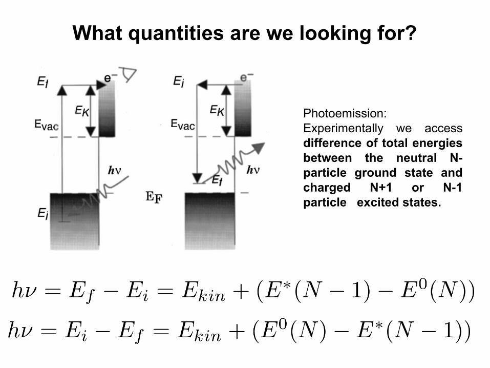
What quantities are we looking for?
Photoemission:Experimentally we access difference of total energies between the neutral N-particle ground state and charged N+1 or N-1 particle excited states.
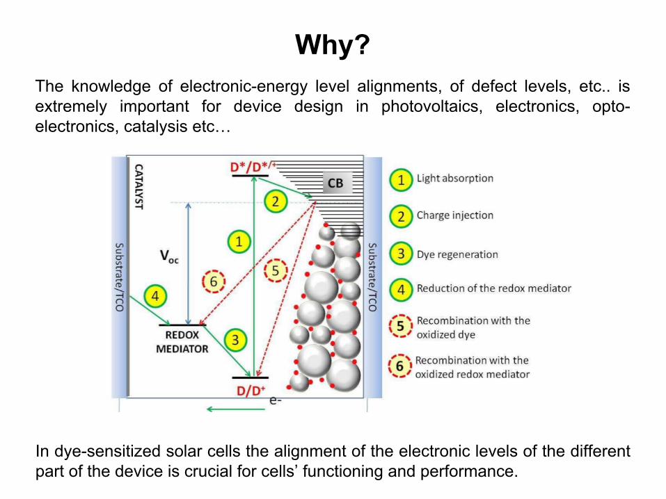
Why?The knowledge of electronic-energy level alignments, of defect levels, etc.. is extremely important for device design in photovoltaics, electronics, opto-electronics, catalysis etc…
In dye-sensitized solar cells the alignment of the electronic levels of the different part of the device is crucial for cells’ functioning and performance.

What kind of systems are we looking at? (1)
Carbon Nanotubes
P. Umari, O. Petrenko, S. Taioli, and M.M. de Souza,J. Chem. Phys.136, 181101 (2012).
Zn-Phthalocyanine
P.Umari and S.Fabris J. Chem. Phys, 136, 174310 (2012)
Organic dyes on TiO2 surfaces
P.Umari, L.Giacomazzi,F. De Angelis, M. Pastore,S. Baroni, JCP 139, 014709 (2013)
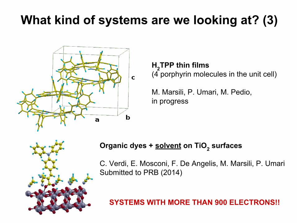
Organic dyes + solvent on TiO2 surfaces
C. Verdi, E. Mosconi, F. De Angelis, M. Marsili, P. UmariSubmitted to PRB (2014)
H2TPP thin films (4 porphyrin molecules in the unit cell)
M. Marsili, P. Umari, M. Pedio, in progress
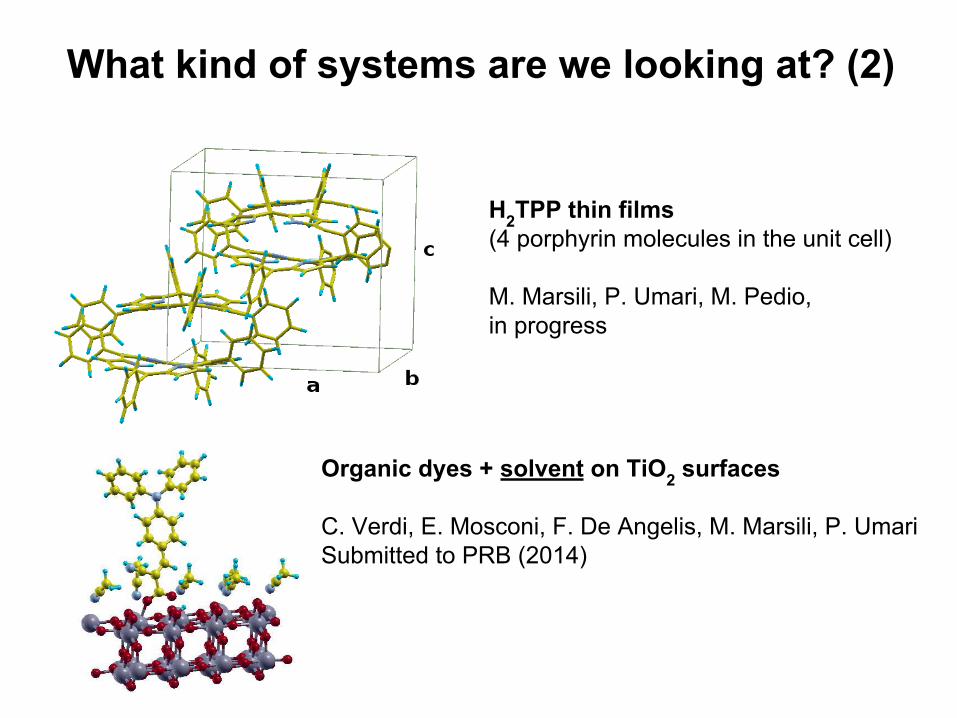
What kind of systems are we looking at? (2)
Organic dyes + solvent on TiO2 surfaces
C. Verdi, E. Mosconi, F. De Angelis, M. Marsili, P. UmariSubmitted to PRB (2014)
H2TPP thin films (4 porphyrin molecules in the unit cell)
M. Marsili, P. Umari, M. Pedio, in progress
SYSTEMS WITH MORE THAN 900 ELECTRONS!!
What kind of systems are we looking at? (3)
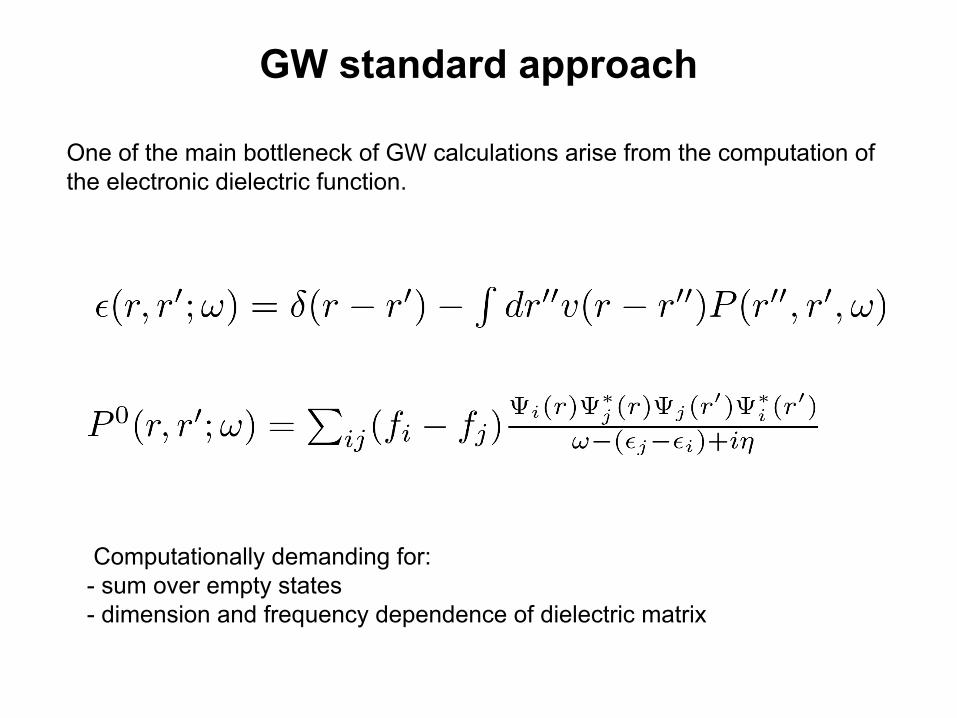
Computationally demanding for:- sum over empty states - dimension and frequency dependence of dielectric matrix
GW standard approach
One of the main bottleneck of GW calculations arise from the computation of the electronic dielectric function.
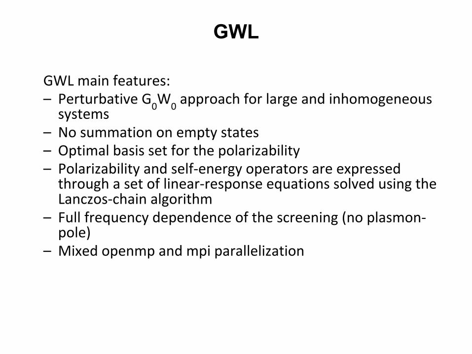
GWL main features:– Perturbative G
0W
0 approach for large and inhomogeneous
systems – No summation on empty states– Optimal basis set for the polarizability– Polarizability and self-energy operators are expressed
through a set of linear-response equations solved using the Lanczos-chain algorithm
– Full frequency dependence of the screening (no plasmon-pole)
– Mixed openmp and mpi parallelization
GWL
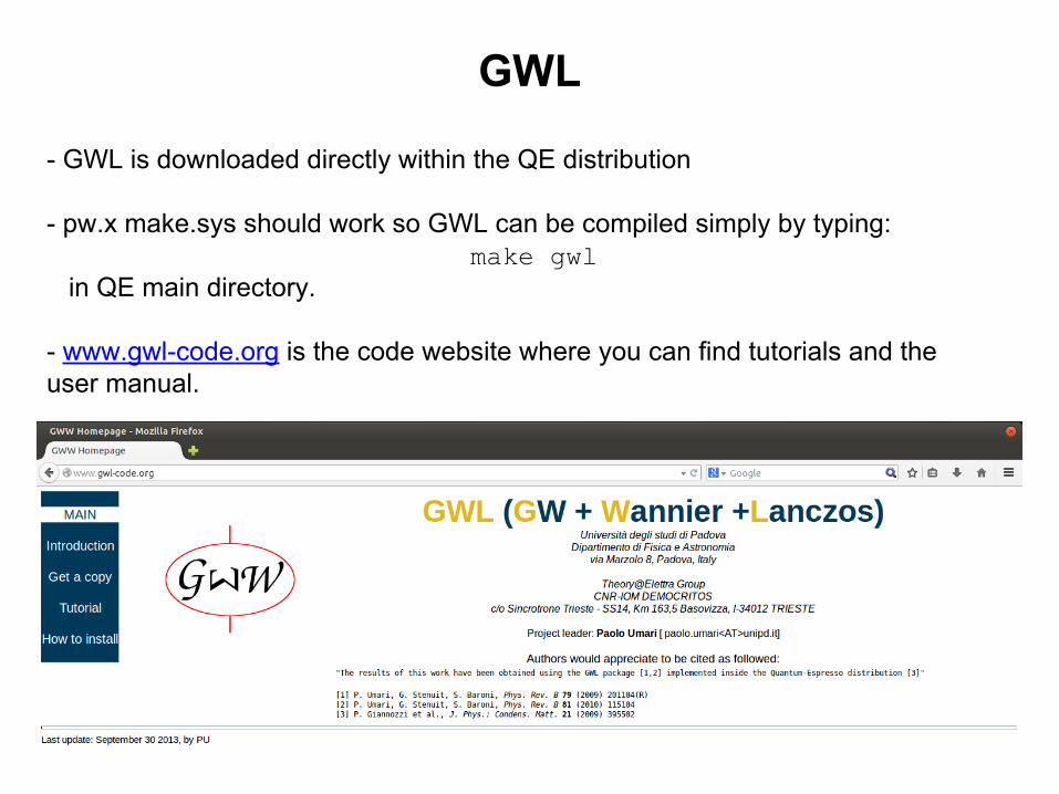
- GWL is downloaded directly within the QE distribution
- pw.x make.sys should work so GWL can be compiled simply by typing:make gwl
in QE main directory.
- www.gwl-code.org is the code website where you can find tutorials and the user manual.
GWL

QP energies (that can be compared with direct and inverse PE) are computed in first order perturbation theory using as perturbation to the KS Hamiltonian.
GW approximation, Wc
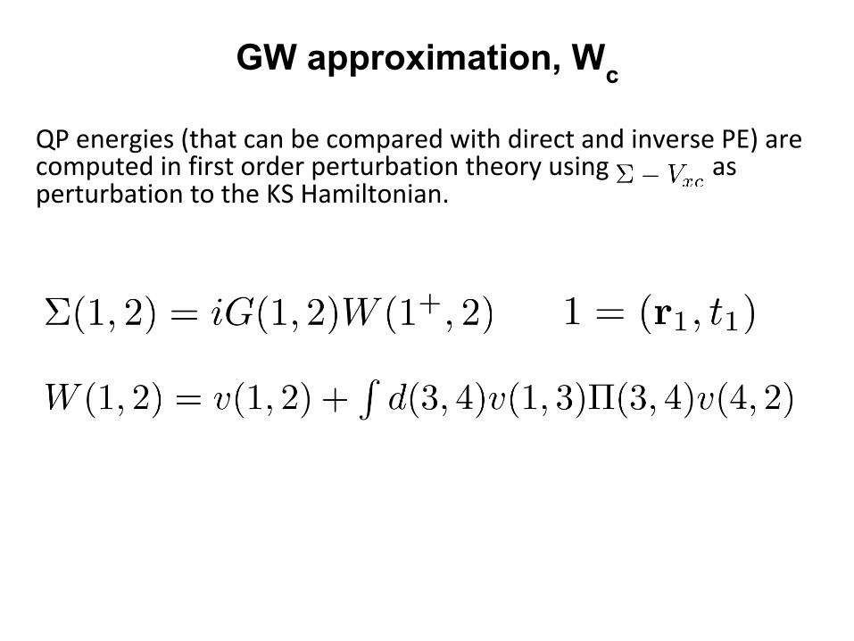
QP energies (that can be compared with direct and inverse PE) are computed in first order perturbation theory using as perturbation to the KS Hamiltonian.
GW approximation, Wc
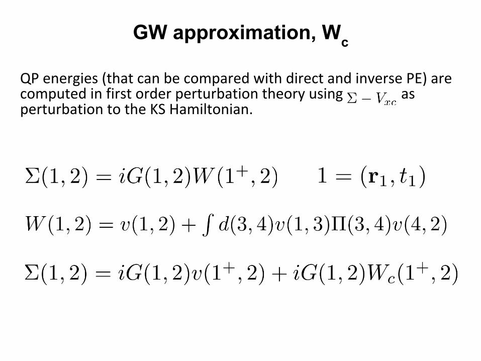
QP energies (that can be compared with direct and inverse PE) are computed in first order perturbation theory using as perturbation to the KS Hamiltonian.
GW approximation, Wc

QP energies (that can be compared with direct and inverse PE) are computed in first order perturbation theory using as perturbation to the KS Hamiltonian.
GW approximation, Wc

Frequency dependence, analytic continuation
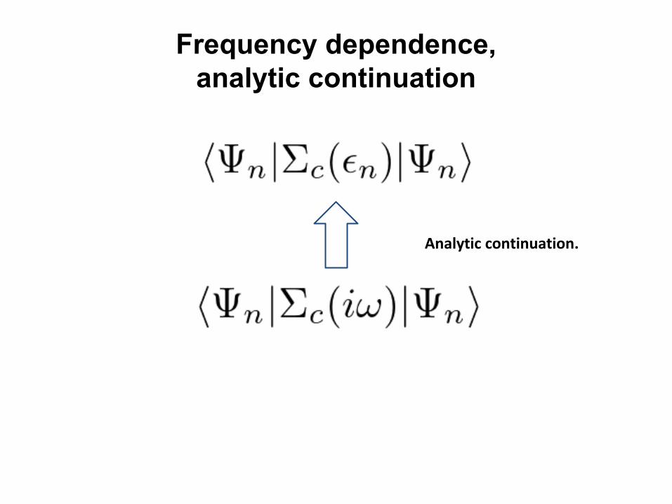
Analytic continuation.
Frequency dependence, analytic continuation
Analytic continuation.
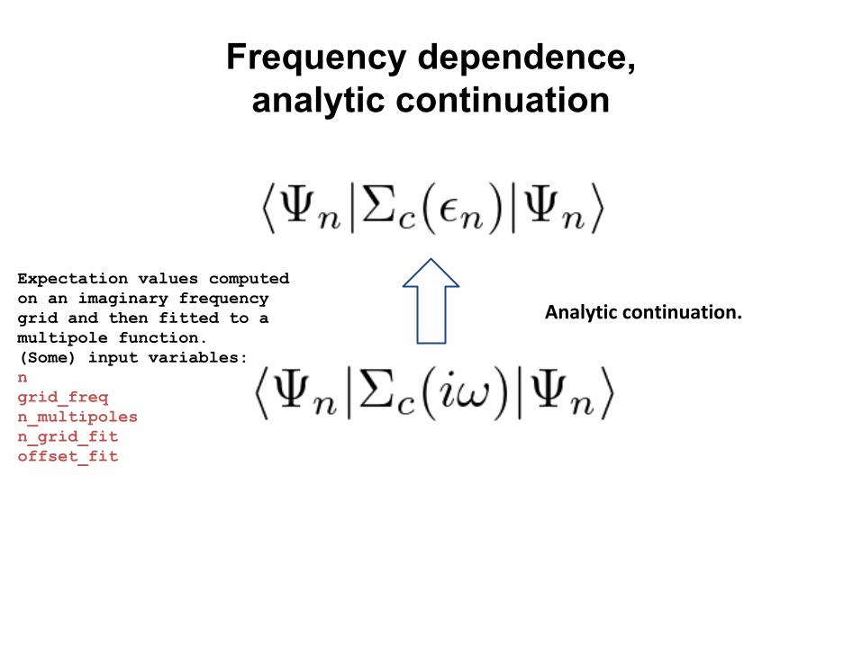
Frequency dependence, analytic continuation
Expectation values computed on an imaginary frequency grid and then fitted to a multipole function.(Some) input variables:ngrid_freqn_multipolesn_grid_fitoffset_fit

Analytic continuation.
Frequency dependence, analytic continuation
FFT
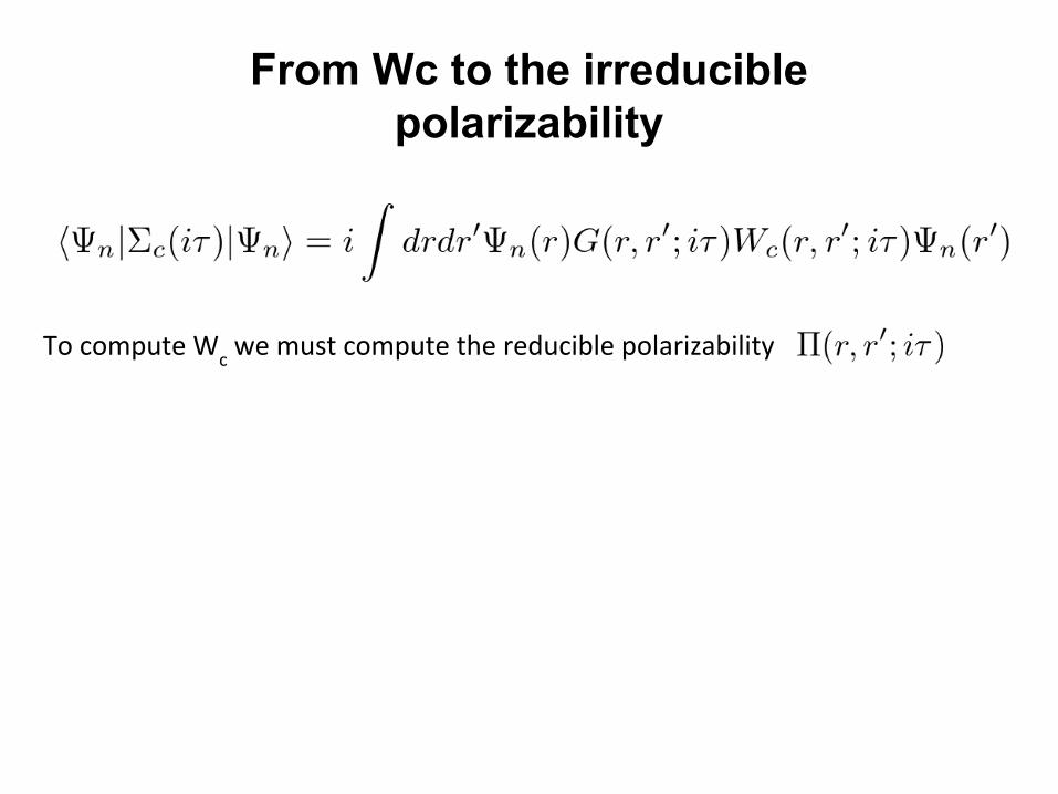
To compute Wc we must compute the reducible polarizability
From Wc to the irreducible polarizability

To compute Wc we must compute the reducible polarizability
Irreducible polarizability
From Wc to the irreducible polarizability
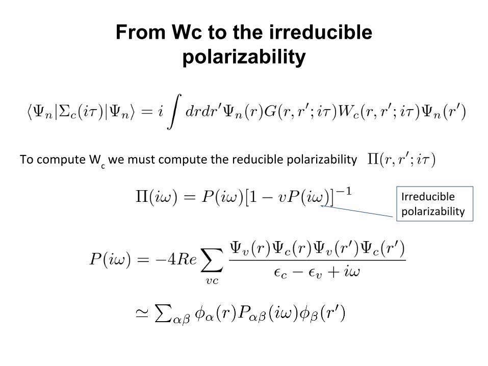
To compute Wc we must compute the reducible polarizability
Irreducible polarizability
From Wc to the irreducible polarizability
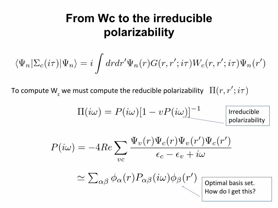
To compute Wc we must compute the reducible polarizability
Irreducible polarizability
Optimal basis set.How do I get this?
From Wc to the irreducible polarizability

To compute Wc we must compute the reducible polarizability
Irreducible polarizability
Optimal basis set.How do I get this?
How do we efficiently compute the matrix elements?
From Wc to the irreducible polarizability

To compute Wc we must compute the reducible polarizability
Irreducible polarizability
Optimal basis set.How do I get this?
From Wc to the irreducible polarizability
How do we efficiently compute the matrix elements?
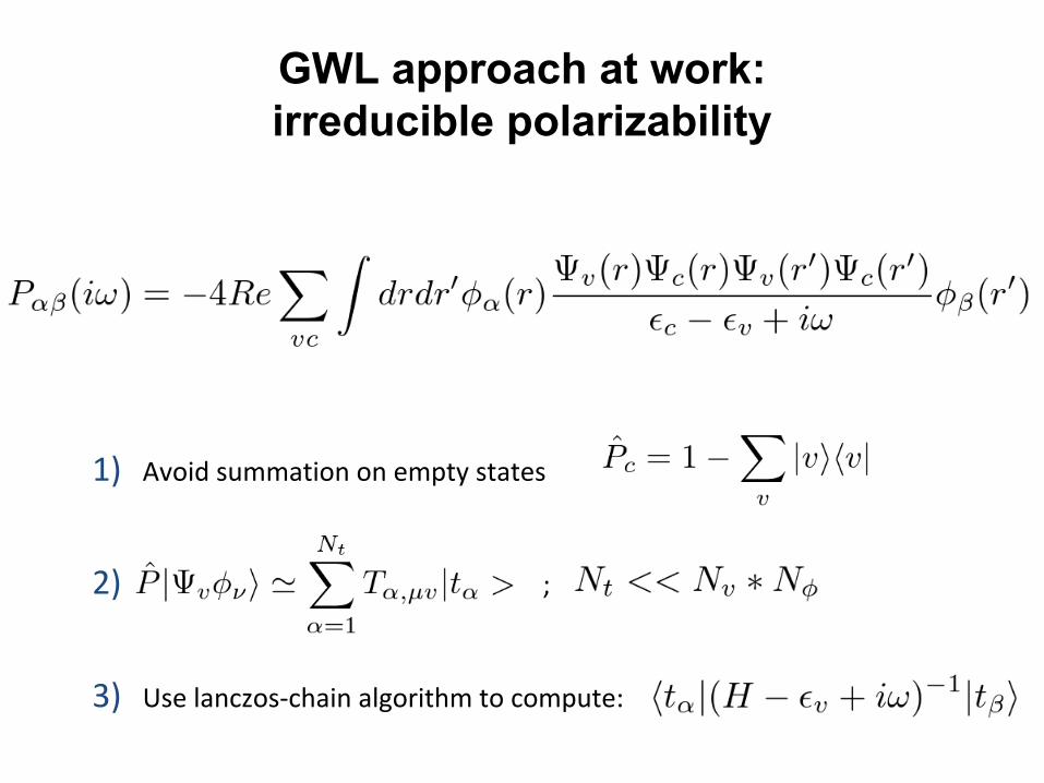
1) Avoid summation on empty states
2) ;
3) Use lanczos-chain algorithm to compute:
GWL approach at work: irreducible polarizability

GWL approach at work: (1) no summation on empty states
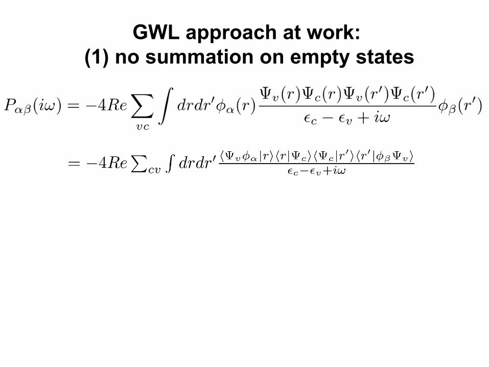
GWL approach at work: (1) no summation on empty states

GWL approach at work: (1) no summation on empty states

GWL approach at work: (1) no summation on empty states
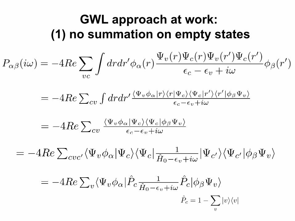
GWL approach at work: (1) no summation on empty states
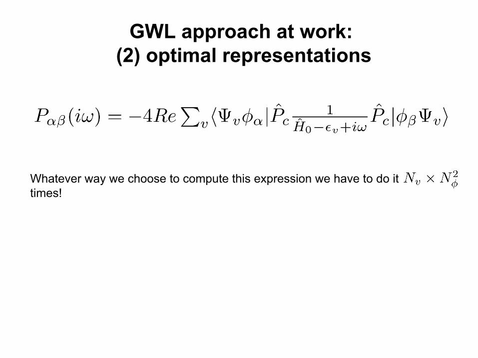
GWL approach at work: (2) optimal representations
Whatever way we choose to compute this expression we have to do it times!

GWL approach at work: (2) optimal representations
Whatever way we choose to compute this expression we have to do it times! The effort is reduced if we find an optimal set of vectors, in terms of which we decompose the vectors belonging to the original set.
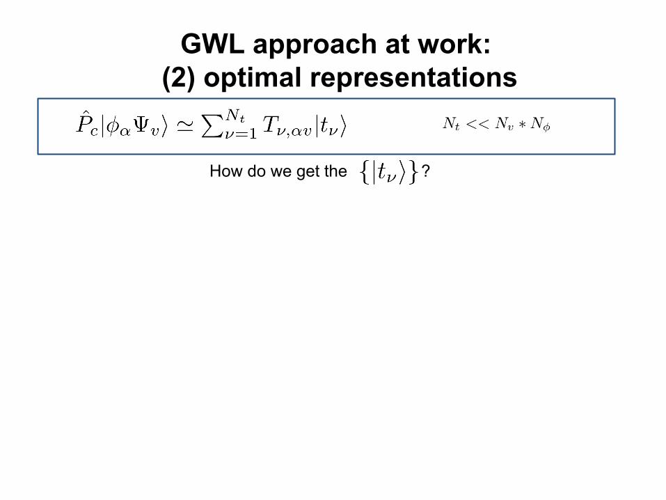
GWL approach at work: (2) optimal representations
How do we get the ?
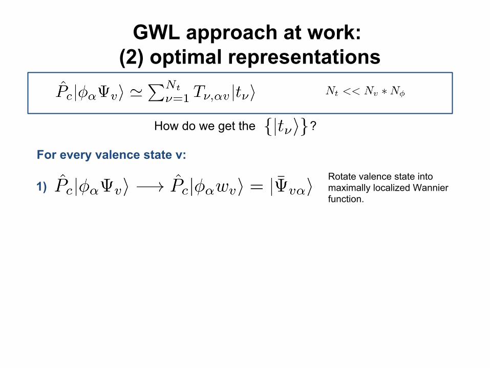
GWL approach at work: (2) optimal representations
How do we get the ?
1)Rotate valence state into maximally localized Wannier function.
For every valence state v:

GWL approach at work: (2) optimal representations
How do we get the ?
1)Rotate valence state into maximally localized Wannier function.
For every valence state v:
2) Compute the overlap matrix

GWL approach at work: (2) optimal representations
How do we get the ?
1)Rotate valence state into maximally localized Wannier function.
For every valence state v:
2) Compute the overlap matrix
3) Solve the eigenvalue problem and keep the Nt eigenvectors with the largest eigenvalues.

GWL approach at work: (2) optimal representations
How do we get the ?
1)Rotate valence state into maximally localized Wannier function.
For every valence state v:
2) Compute the overlap matrix
3) Solve the eigenvalue problem and keep the Nt eigenvectors with the largest eigenvalues.
This procedure is called singular value decomposition (SVD). Important input variable: n_pola_lanczos it defines the number of eigenvectors to be kept.

GWL approach at work: (2) optimal representations
We are still left with Nv blocks made of Nt “local” t states!

GWL approach at work: (2) optimal representations
We are still left with Nv blocks made of Nt “local” t states!
4) We perform an other SVD among the blocks keeping the eigenvectors with eigenvalue above a threshold value s.
Important input variable: s_pola_lanczos
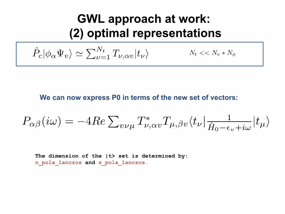
GWL approach at work: (2) optimal representations
We can now express P0 in terms of the new set of vectors:
The dimension of the |t> set is determined by:n_pola_lanczos and s_pola_lanczos.
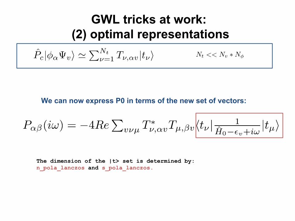
GWL tricks at work: (2) optimal representations
We can now express P0 in terms of the new set of vectors:
The dimension of the |t> set is determined by:n_pola_lanczos and s_pola_lanczos.
GWL approach at work: (3) lanczos chain algorithm
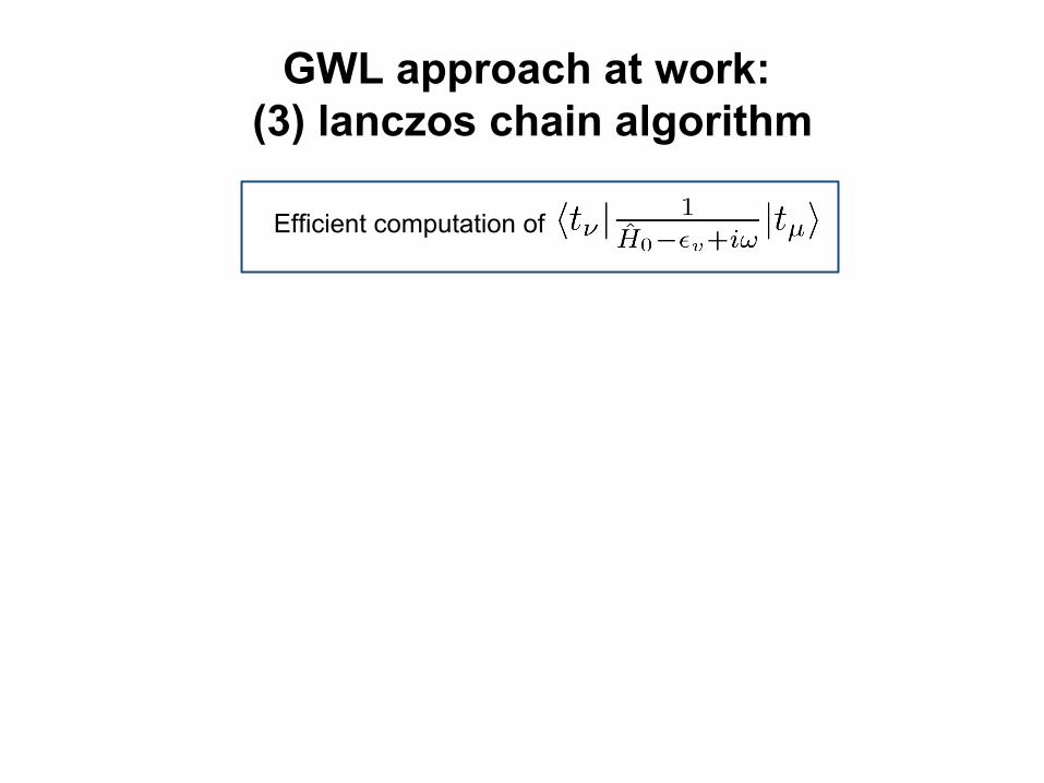
Efficient computation of
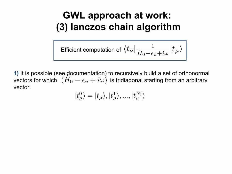
GWL approach at work: (3) lanczos chain algorithm
Efficient computation of
1) It is possible (see documentation) to recursively build a set of orthonormal vectors for which is tridiagonal starting from an arbitrary vector.
GWL approach at work: (3) lanczos chain algorithm
Efficient computation of
1) It is possible (see documentation) to recursively build a set of orthonormal vectors for which is tridiagonal starting from an arbitrary vector.
2) Compute
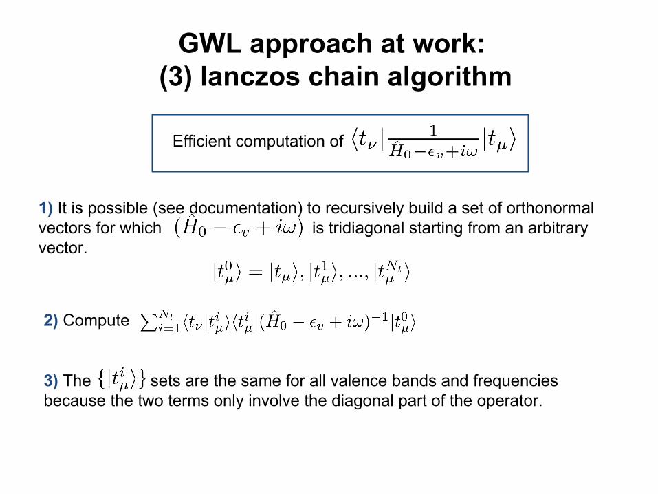
GWL approach at work: (3) lanczos chain algorithm
Efficient computation of
1) It is possible (see documentation) to recursively build a set of orthonormal vectors for which is tridiagonal starting from an arbitrary vector.
2) Compute
3) The sets are the same for all valence bands and frequencies because the two terms only involve the diagonal part of the operator.

GWL approach at work: (2) lanczos chain algorithm
Efficient computation of
1) It is possible (see documentation) to recursively build a set of orthonormal vectors for which is tridiagonal starting from an arbitrary vector.
2) Compute
3) The sets are the same for all valence bands and frequencies because the two terms only involve the diagonal part of the operator.
This procedure is part of the so called Lanczos-chain algorithm. Important input variable: n_steps_lanczos_pola, it determines the dimension of the vectors chain.

Optimal representation of the dynamical polarizability (1)
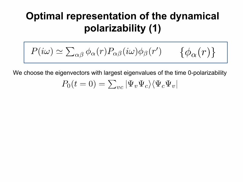
Optimal representation of the dynamical polarizability (1)
We choose the eigenvectors with largest eigenvalues of the time 0-polarizability

Optimal representation of the dynamical polarizability (1)
1) SVD on
namely solve
We choose the eigenvectors with largest eigenvalues of the time 0-polarizability
In principle

Optimal representation of the dynamical polarizability (1)
1) SVD on
namely solve
2)
We choose the eigenvectors with largest eigenvalues of the time 0-polarizability
In principle

Optimal representation of the dynamical polarizability (1)
1) SVD on
namely solve
2)
We choose the eigenvectors with largest eigenvalues of the time 0-polarizability
In principle
This requires a great number of conduction states to be computed!

Optimal representation of the dynamical polarizability (2)

Optimal representation of the dynamical polarizability (2)
1) Consider “fake” conduction states, namely: planewaves below a certain threshold projected onto the conduction manifold.

Optimal representation of the dynamical polarizability (2)
1) Consider “fake” conduction states, namely: planewaves below a certain threshold projected onto the conduction manifold.
2) Use max. loc. Wannier functions

Optimal representation of the dynamical polarizability (2)
1) Consider “fake” conduction states, namely: planewaves below a certain threshold projected onto the conduction manifold.
2) Use max. loc. Wannier functions
3) Gram-Schmidt orthonormalize and keep the vectors whose norm is above a certain threshold s.
4) Diagonalize and keep the Np eigenvectors with the largest eigenvalues.
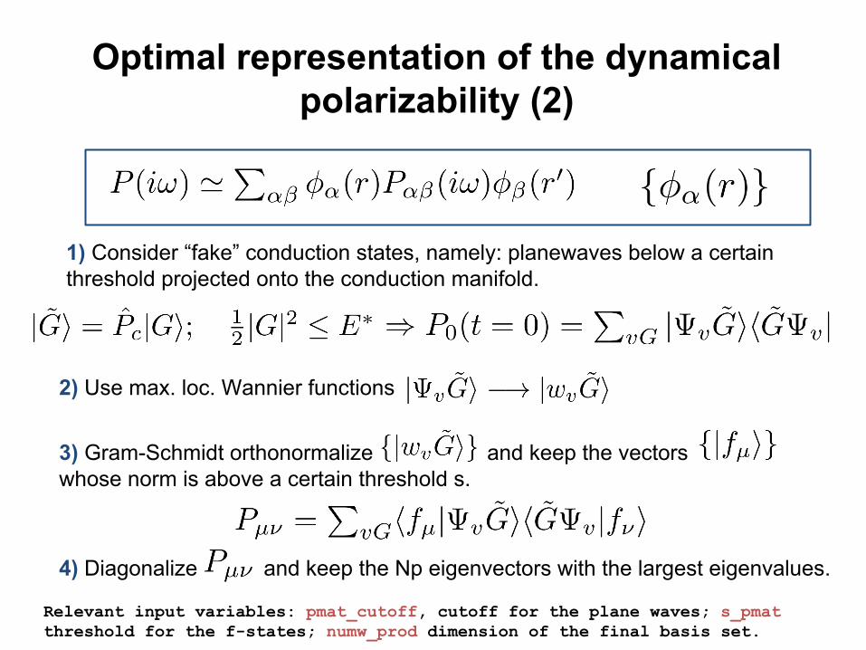
Relevant input variables: pmat_cutoff, cutoff for the plane waves; s_pmat threshold for the f-states; numw_prod dimension of the final basis set.
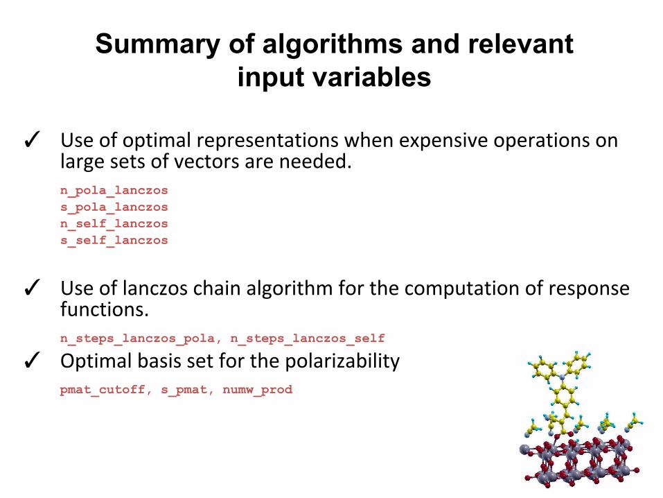
Summary of algorithms and relevant input variables
✓ Use of optimal representations when expensive operations on large sets of vectors are needed.n_pola_lanczoss_pola_lanczosn_self_lanczoss_self_lanczos
✓ Use of lanczos chain algorithm for the computation of response functions.n_steps_lanczos_pola, n_steps_lanczos_self
✓ Optimal basis set for the polarizabilitypmat_cutoff, s_pmat, numw_prod

Thank you, references, acknowledgments
USER MANUAL: http://www.gwl-code.org/manual_gwl.pdf
GW APPROXIMATION: L. Hedin and S. Lundqvist. Solid State Phys., 23:1, 1970.F. Aryasetiawan, O. Gunnarsson, Rep. Prog. Phys. 61 (3): 237 (1998).
ANALYTIC CONTINUATION TECHNIQUE:H. N. Rojas, R. W. Godby, and R. J. Needs. Phys. Rev. Lett., 74, 1827, (1995)M. M. Rieger, L. Steinbek, I. D. White, H. N. Rojas, and R. W. Godby. Comput. Phys. Commun., 117, 211, (1999)
GWL NUMERICAL APPROACH:P. Umari, G. Stenuit, and S. Baroni. Phys. Rev. B, 79:201104(R), 2009.P. Umari, G. Stenuit, and S. Baroni. Phys. Rev. B, 81:115104, 2010.
Dott. Paolo Umari, Università di PadovaGWL main developer
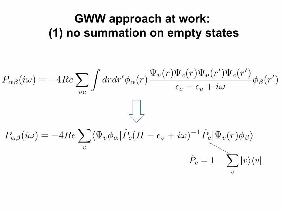
GWW approach at work: (1) no summation on empty states
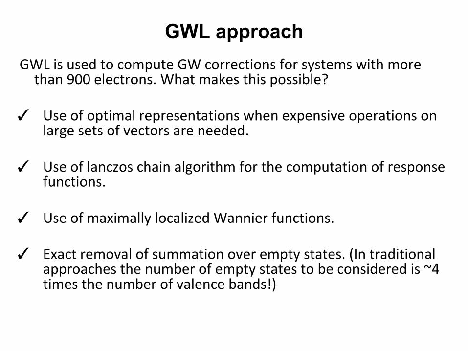
GWL is used to compute GW corrections for systems with more than 900 electrons. What makes this possible?
✓ Use of optimal representations when expensive operations on large sets of vectors are needed.
✓ Use of lanczos chain algorithm for the computation of response functions.
✓ Use of maximally localized Wannier functions.
✓ Exact removal of summation over empty states. (In traditional approaches the number of empty states to be considered is ~4 times the number of valence bands!)
GWL approach


