

The Lifetime Earnings Premia of Di�erent Majors:
Correcting for Selection Based on Cognitive,
Noncognitive, and Unobserved Factors
Douglas A. Webber∗†
June 9, 2014
∗Temple University Department of Economics and IZA. 1301 Cecil B. Moore Ave. Ritter Annex 883.Philadelphia, PA. 19102 Email: [email protected]†I have greatly bene�ted from the advice of J. Catherine Maclean, Ron Ehrenberg, Ben Ost, and Moritz
Ritter.
1 Introduction
With average U.S. college tuition continuing to rise at a rate roughly 3.5 percentage points
faster than in�ation (Ehrenberg, 2012), graduating high school seniors face the prospect
of taking on substantial student loan debt only to be confronted with an uncertain and
turbulent labor market after graduating from college. It is therefore more important than
ever for students to have accurate information not just about the value of a generic college
degree, but also about the relative economic returns to di�erent majors.
Recent work has focused on the role that students' expectations play in the decision of
whether to attend and what to study in college. While there is certainly a large literature
devoted to estimating the college premium after controlling for unobserved ability, the results
are typically focused on an economy-wide average or a point in the life-cycle estimate (e.g.
age 30) rather than on the lifetime earnings premium. This is an important distinction as
education-speci�c earnings pro�les di�er across age groups. I also document the importance
of accounting for job search behavior (di�erential unemployment across majors). Finally,
to the best of my knowledge the lifetime college premium (adjusting for ability sorting) has
never been broken down across majors1.
I use data from the National Longitudinal Study of Youth 1979 cohort (NLSY) and the
American Community Survey (ACS) to construct lifetime earnings trajectories for individu-
als in several di�erent degree categories (Social Sciences, Science/Technology/Engineering/Math,
Arts and Humanities, and Business), as well as those with only a high school diploma or
some college experience but no 4-year degree. The trajectories are generated from a sim-
ulation approach which combines lifecycle earnings paths and degree choice (NLSY) with
current degree premiums (ACS). Since there is a high degree of selection associated with
both educational attainment and degree choice, I use a method employed by Taber (2001)
to infer the magnitude of selection bias for each major category at all points of the life-cycle.
1See Walker and Zhu (2011) for an excellent example of lifetime earnings decomposed by major withoutaccounting for endogenous major choice.

The simulated earnings trajectories are then adjusted to account for the magnitude of self-
selection. Additionally, I employ a bounding method proposed by Altonji et al. (2005) to
evaluate various assumptions regarding the degree of selection on unobservables of major
choice.
Taber's method for backing out the selection bias is relatively straightforward: Estimate
an earnings premium (Taber considered the premium to having a college diploma using
the NLSY) either unconditionally or controlling only for basic demographic characteristics.
Next, estimate the premium while controlling for ability and factors which might drive
selection (Test scores, mother's education, etc.). The di�erence between the two earnings
premia is an estimate of the degree of self-selection. I make use of the often-studied Armed-
Forces Quali�cation Test (AFQT) score from the NLSY, as well as the noncognitive ability
measures including the Rotter Scale and Rosenberg Self-Esteem Score, to estimate the degree
of self selection for each �eld of study. Furthermore, I utilize the cognitive and noncognitive
ability measures to separately address several types of selection (selection into attending
college, selection into major, time to completing the degree, and probability of completing
the degree).
I �nd that accounting for selection substantially alters the expected lifetime earnings
premia associated with each education group examined. I estimate signi�cant heterogeneity
in the return to various majors after accounting for observable selection through cognitive
and noncognitive ability. I �nd that Arts/Humanities graduates receive on average $700,000
more than high school graduates with no college experience over the course of their lifetimes
holding cognitive and noncognitive ability measures constant. Social Science graduates re-
ceive an analogous premium of $1.05 million, Business majors receive a premium of about
$1.4 million, and STEM graduates realize the largest premium of $1.5 million. Each premium
varies with the inclusion or exclusion of job search behavior, with STEM gradatues having
the greatest likelihood of being employed full-time throughout an entire year. Furthermore,
I �nd that this heterogeneity in returns persists under plausible magnitudes of unobservable
2
selection.
Finally, by imposing an assumption on the shape of lifecycle earnings, I can estimate the
returns to each major separately across three birth cohorts (1955-64, 1965-74, and 1975-84).
I �nd that there has been a moderate convergence over time in the return to the various
major categories.
From a policy perspective, this work has implications in several �elds. In the student
loan literature, a more detailed understanding of the economic returns to di�erent majors
can inform how interest rates are set and how loans are subsidized by the government.
Additionally, there has been a recent push in some state legislatures (e.g. Florida and North
Carolina) to explore charging di�erential tuition by major at public universities. The lifetime
premium to di�erent majors should certainly enter into the equation which universities use
to determine how to set these tuition levels.
The paper is constructed as follows. Section 2 discusses the previous literature. Section
3 describes the data used to construct the lifetime earnings trajectories. Section 4 details
the empirical methodology used in the simulations. Section 5 provides a discussion of the
�ndings and their implications, and Section 6 concludes.
2 Background
Estimating the returns to education is one of the oldest and most detailed literatures in
empirical economics (see Card (1999) for a review). In accordance with the nonlinear impact
of years of education on earnings, many studies have focused on the returns speci�c to
discrete units of schooling such as a high school diploma or a 4-year college degree (Averett
and Burton (1996); Brewer et al. (1999); Goldin and Katz (2008); Grogger and Eide (1995);
Dillon (2012) to name just a few). For an extensive review of the curriculum and college
major choice literatures, see the excellent article by Altonji. et al. (2012).
3

Much of the literature on college major choice focuses on the role of expected earnings
in students' decisions. While the general consensus is that expected future earnings play a
large part in major choice, a variety of di�erent methods are used to arrive at this conclusion.
Berger (1988) uses a Heckman selection framework to control for self-selection into majors
and produces an estimate of the short-term expected future earnings from each degree. He
uses family background characteristics as exclusion restrictions from the earnings equation.
The predicted earnings from the Heckman model is then included in a conditional logit model
of college choice, and is found to be a signi�cant factor in students' decisions.
Using a dynamic discrete-choice framework, Arcidiacono (2004) �nds that expected earn-
ings play a role in major choice, although less than that found in Berger (1988). Furthermore,
Arcidiacono (2004) �nds evidence that the exclusion restrictions used in Berger (1988) may
be invalid. In a more recent study of Duke University undergraduates, Arcidiacono et al.
(2012) concludes that much of the selection into majors is due to comparative advantage (i.e.
students choose the major which maximizes future earnings subject to their unique mix of
skills, as in a standard Roy model framework; Roy (1951)). Montmarquette et al. (2002) �nd
a strong impact of expected earnings upon graduation from college (which accounts for both
the earnings of recent graduates and the probability of completing a given degree) in their
model of major choice, which also accounts for relative major premiums and the likelihood
of completing a given major.
Another branch of the college premium literature focuses on the di�erential returns to
speci�c skills learned in college rather than majors. Grogger and Eide (1995) document
the growing importance of math ability in explaining earnings di�erences, decomposing this
e�ect into both the return to math ability and the change in the composition of college
graduates' �eld of degree. Hamermesh and Donald (2008) demonstrate that holding college
major constant, there are substantial returns to taking upper-division science and math
courses. This work is particularly relevant to the current study, as it provides evidence
of di�erential human capital growth across majors, and thus a clear mechanism to explain
4

di�erential lifetime earnings premiums across college majors.
Robst (2007) provides evidence that there can be signi�cant wage penalties for workers
employed in �elds di�erent from their college major. This could lead to di�erences in the
returns to college majors if there are di�erential shifts in the supply/demand for each major,
thus forcing some majors to work in outside �elds more than others.
In sum, the literature suggests that there will be di�erential lifetime wage premia to
di�erent degrees. However, the size of such premia and the importance of selection is un-
known. The analyses performed in this paper serve as an important complement to this
growing literature on major choice and the di�erential returns to majors.
3 Data
I use two datasets used to construct the lifetime earnings trajectories in this study, the 1979
cohort of the National Longitudinal Survey of Youth (NLSY) and the American Community
Survey (ACS).
The NLSY is a panel dataset which began surveying 12,686 individuals annually between
1979 and 1994 and biennially between 1994 and the present. All respondents were between
the ages of 14 and 22 during the initial survey year of 1979. The NLSY is quite broad in its
scope of survey questions, and has been used countless times in the economics literature. It
was designed in part to track the transition from school to work, and thus is well-suited for
the current study. One of the most appealing attributes of the NLSY is the availability of
cognitive ability measures. The Armed Forces Quali�cation Test (AFQT) is a composite per-
centile rank of four subsections of the Armed Forces Vocational Aptitude Battery (ASVAB):
word knowledge, paragraph comprehension, arithmetic reasoning, and mathematics knowl-
edge. Given its construction, the AFQT is comparable to standard college entrance test
scores. The NLSY also contains data on two commonly used measures of noncognitive abil-
5
ity, the Rotter Scale which gauges locus of control and the Rosenberg Self-Esteem Score. An
individual with a high score on the Rotter Scale believes their actions have little impact on
the quality of their life, and has commonly been used as a measure of noncognitive skill in the
labor literature (Osborne-Groves, 2005; Heckman et al., 2006). The Rosenberg Scale repre-
sents an individual's assessment of their self-esteem or self worth. While it is less commonly
used than the Rotter Scale, it is also seen as a viable measure of noncognitive abilities in the
education and labor literatures (Murnane et al., 2001; Heckman et al., 2006). As discussed
in Heckman et al. (2006), these variables are important components of the education selec-
tion mechanism. Since the measures of cognitive and noncognitive ability were measured
only once for each individual between 1979 and 1981, I must make the assumption that the
economic impact of these qualities remains relatively constant over time. Fortunately, recent
research supports this assumption (Cobb-Clark and Schurer, 2013).
The ACS is a large-scale nationally representative survey which is designed to replace the
decennial long-form Census. It provides data on more than 3 million individuals every year,
and allows for much �ner geographic identi�ers than any other national survey. The appeal
of using the ACS as opposed to other national surveys is twofold. First, the ACS recently
began asking respondents their major �eld of study if they attended college. Second, the
large sample sizes for even narrow age group and major category bins allows for the precise
estimation of regression coe�cients.
There are six educational outcomes examined in this paper: high school graduates with
no college experience, some college but no four-year degree, and four-year degrees in science
technology engineering or math (STEM), Business, Social Science, and Arts/Humanities.
These categories are chosen to be broad enough to estimate precise di�erences in both the
NLSY and ACS parameters. A complete accounting of each major can be found in the NLSY
documentation2. Below are the NLSY major category groupings which I include in each bin
for the purposes of this paper:
2http://www.nlsinfo.org/content/cohorts/nlsy79/other-documentation/codebook-supplement/nlsy79-attachment-4-�elds-study. Access date 4/23/2013
6

STEM - Biological Sciences, Computer and Information Sciences, Engineering, Health Pro-
fessions, Mathematics, Physical Sciences
Business - Business and Management
Social Science - Social Sciences, Psychology
Arts and Humanities - Theology, Letters, Library Science, Fine and Applied Arts, Foreign
Languages, Architecture
This list is obviously not collectively exhaustive, and thus all majors not included in
the above �elds are categorized as �other� and included in each regression model as such.
The �other� category includes majors such as military science, education3, area studies, or
interdisciplinary studies. This paper does not report results for the �other� category because
of the dissimilar nature of the degrees contained in that group, however it is important to
include this outcome as a regressor in each model so that each of the college-level educational
outcomes are collectively exhaustive.
There are several sample restrictions made for both the NLSY and ACS datasets in order
to construct an appropriate sample. First, only men are included in the analysis sample,
consistent with many labor market studies. This is a particularly important restriction for
this study given the relatively weaker labor force attachment of women in the 1979 cohort
of the NLSY and the drastic di�erences in major choice among women (e.g. STEM �elds)
relative to today. Any individuals currently enrolled in school or the military are dropped.
Only individuals age 18-64 are studied. In order to construct the most relevant comparison
group, individuals with less than a high school diploma or any advanced college degrees are
excluded from the analyses. This exclusion may understate the value of a particular major
because it removes the option value of attending graduate school (see Eide and Waehrer
(1998) for a discussion of the option value of graduate school). Finally, individuals are
3Education was not studied as a major category in this paper because many states require some post-graduate work to be certi�ed as a teacher long-term. Including individuals with post-graduate work wouldintroduce a large degree of endogeneity into the estimates due to selection. Not including these individu-als but still looking at education majors would produce a substantial underestimate of the returns to aneducation degree.
7
only retained in the sample if they have positive earnings over the previous year. This
condition may lead to an understatement of each college premium because it necessarily
removes the long-term unemployed from the sample. However, including these individuals
would introduce considerable bias into the results given that extremely weak labor force
attachment is likely unobservably correlated with schooling decisions.
The �nal NLSY sample is comprised of 3,943 men (51,377 person-year observations), while
the ACS sample covers 475,896 men. Sample weights are used in each analysis presented in
this paper.
4 Empirical Model
The key contribution of this paper is to simulate selection-corrected earnings trajectories for
various college majors. This section outlines the necessary components for conducting these
simulations.
Magnitude of Self-Selection
Both cognitive and noncognitive abilities play a large role in the choice of college major
(Heckman et al., 2006). Given the strong positive link between these factors and wages,
failure to account for cognitive and noncognitive measures will lead to an overstatement of
the returns to education. The NLSY's detailed set of variables provides the ideal setting to
measure the magnitude of this self-selection.
Using the NLSY sample, the following regressions are estimated:
yij = α0 + α1Ageij + α2Blacki + α3Hispi + γEduci + εij (1)
8
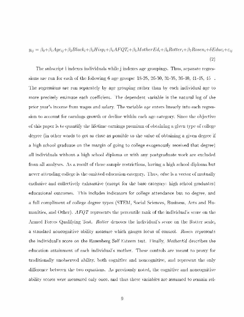
yij = β0+β1Ageij+β2Blacki+β3Hispi+β4AFQTi+β5MotherEdi+β6Rotteri+β7Roseni+δEduci+εij
(2)
The subscript i indexes individuals while j indexes age groupings. Thus, separate regres-
sions are run for each of the following 6 age groups: 18-25, 26-30, 31-35, 36-40, 41-45, 45+.
The regressions are run separately by age grouping rather than by each individual age to
more precisely estimate each coe�cient. The dependent variable is the natural log of the
prior year's income from wages and salary. The variable age enters linearly into each regres-
sion to account for earnings growth or decline within each age category. Since the objective
of this paper is to quantify the lifetime earnings premium of obtaining a given type of college
degree (in other words to get as close as possible to the value of obtaining a given degree if
a high school graduate on the margin of going to college exogenously received that degree)
all individuals without a high school diploma or with any postgraduate work are excluded
from all analyses. As a result of these sample restrictions, having a high school diploma but
never attending college is the omitted education category. Thus, educ is a vector of mutually
exclusive and collectively exhaustive (except for the base category: high school graduates)
educational outcomes. This includes indicators for college attendance but no degree, and
a full compliment of college degree types (STEM, Social Sciences, Business, Arts and Hu-
manities, and Other). AFQT represents the percentile rank of the individual's score on the
Armed Forces Qualifying Test. Rotter denotes the individual's score on the Rotter scale,
a standard noncognitive ability measure which gauges locus of control. Rosen represents
the individual's score on the Rosenberg Self-Esteem test. Finally, MotherEd describes the
education attainment of each individual's mother. These controls are meant to proxy for
traditionally unobserved ability, both cognitive and noncognitive, and represent the only
di�erence between the two equations. As previously noted, the cognitive and noncognitive
ability scores were measured only once, and thus these variables are assumed to remain rel-
9

atively constant over time (an assumption supported by Cobb-Clark and Schurer (2013)).
Additionally, the AFQT scores are normalized by the age at which the test was taken to
account for age-related bias (Heckman et al. (2006)).
I experimented with the control variables entering into the model in various less para-
metric functional forms (e.g. including higher order polynomials, dummy variables for each
decile, etc.). There was surprisingly little di�erence in the estimated education parameters
across these speci�cations. The results presented in this paper are therefore based on the
most parsimonious model where each variable enters linearly into the log earnings regressions,
however other results are available upon request.
The relatively parsimonious nature of Equations (1) and (2) is intentional, and is meant
to avoid controlling for factors which are outcomes of educational choice but also in�uence
earnings. For example, industry and occupation are often outcomes of major choice, and
their inclusion in the model would therefore bias the estimated major premia. Thus, only a
basic set of pre-market factors are included in each model.4
Taking the di�erence of the corresponding education coe�cients from each model (i.e.
δSTEM,jSelection = γSTEM,j − δSTEM,j) yields an estimate of the selection bias usually present when
we estimate education earnings premiums. These selection biases will be used later to adjust
estimated earnings premiums from the ACS, which have no suitable proxies for ability.
The use of the AFQT percentile is attractive because of its straightforward construction
and interpretation (e.g. moving up one percentile in the ability distribution). While this
measure is certainly not a perfect barometer of cognitive ability, it explains roughly ten
percent of the variation in yearly income all by itself5 and is a mainstay in the education
literature.
There are two other models estimated on the NLSY sample which yield information on
4Geographic region (for the NLSY models) and state �xed-e�ects (for the ACS models) were also includedas a robustness check. There are valid arguments both for the inclusion and exclusion of geographic controls.I see no substantive di�erences in the �nal results depending on their inclusion, and thus choose to omitthem from the results presented in the paper to present the most parsimonious model possible.
5Author's calculation based on regression sample used for this paper.
10

several types of selection which can be built into the simulation model. First, an ordered
logit which estimates the contribution of AFQT percentile to likelihood of attending and
completing college.
P (educi = k) = P (ck−1 < Xiβ < ck) (3)
Where education may take on three values (high school diploma without any college,
some college without a degree, any college degree), X is a vector consisting of race, ethnicity,
AFQT score, Rotter Scale, Rosenberg Self-Esteem Score, and mother's education. Each ck
represents a cutpoint (by convention, c0 = −∞ and ck =∞).
Second, I estimate a multinomial logit of the contribution of AFQT percentile to major
choice conditional on earning a college degree.
P (major = k) =eXβ
(k)
1 +∑5k=1 e
Xβ(k))(4)
Where in this case k varies between the 5 major choices studied (Social Sciences, Busi-
ness, STEM, Arts and Humanities, and Other), X is a vector consisting of race, ethnicity,
AFQT score, Rotter Scale, Rosenberg Self-Esteem Score, and mother's education. As in
all multinomial logit estimations6, the coe�cients for one outcome (in this case Other) are
normalized to zero.
The results from these two models are used in the earnings simulation to determine the
level and major (if the individual is assigned to be a college graduate) of each individual.
6The multinomial logit estimator also imposes the well-known Independence of Irrelevant Alternatives(IIA) assumption. Montmarquette et al. (2002) provides evidence that this assumption is satis�ed forapplications to college major choice.
11

Unadjusted earnings paths
Using the 2011 ACS, Equation (5) is run for each of 9 age groups (18-25, 26-30, 31-35, 36-40,
41-45, 46-50, 51-55, 56-60, 61-64).
yij = β0 + β(j)1 ageij + β2Blacki + β3Hispanici + δeduci + εij (5)
Where the dependent variable is the natural log of prior year earnings, and all independent
variables are de�ned as described above. The coe�cient on each education category within
each age grouping, as well as the variance of residual log earnings, σ2educ,j, for each education
category and age grouping are saved. Additionally, I save the mean and variance of log
wages for workers with only a high school diploma to use as a baseline to compare the major
premias.
Life-Cycle Earnings Simulation
Normal cumulative distribution functions (CDFs) are generated for each educational outcome
(High school graduate w/o any college, some college w/o degree, and each major type) and
age grouping based on the coe�cients from Equation (5) and the variance of the residuals
from each group.
Finally, a dataset is populated with 100,000 simulated workers who are randomly assigned
an ability level (1-100) and two uniform random shocks (one to go with the ordered logit
and one for the multinomial logit).
An individual is assigned a schooling level (high school some college, or college degree)
based on the parameters estimated from the conditional logit as well as the ability and the
�rst random shock values. Those with conditional logit scores in percentiles 64-100 of the
distribution are assigned to have completed their degree in 4 years, 54-64 in 5 years, and 44-
12
54 in 6 years. These numbers were chosen to match recent four, �ve, and six-year graduation
rates from U.S. four-year institutions (IPEDS).
For those assigned to be college graduates, the coe�cients on AFQT from the multinomial
logit run on the NLSY sample are used in conjunction with the other random shock to assign
a major to each graduate.
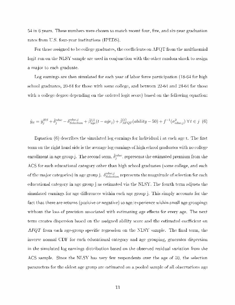
Log earnings are then simulated for each year of labor force participation (18-64 for high
school graduates, 20-64 for those with some college, and between 22-64 and 24-64 for those
with a college degree depending on the ordered logit score) based on the following equation:
yit = yHSj + δeducj − δeduc,jSelection + β(j)age(t− ¯agej) + β
(j)AFQT (ability− 50) + f−1(σ2
educ,j) ∀ t ∈ j (6)
Equation (6) describes the simulated log earnings for individual i at each age t. The �rst
term on the right hand side is the average log earnings of high school graduates with no college
enrollment in age group j. The second term, δeducj , represents the estimated premium from the
ACS for each educational category other than high school graduates (some college, and each
of the major categories) in age group j. δeduc,jSelection represents the magnitude of selection for each
educational category in age group j as estimated via the NLSY. The fourth term adjusts the
simulated earnings for age di�erences within each age group j. This simply accounts for the
fact that there are returns (positive or negative) to age/experience within small age groupings
without the loss of precision associated with estimating age e�ects for every age. The next
term creates dispersion based on the assigned ability score and the estimated coe�cient on
AFQT from each age-group speci�c regression on the NLSY sample. The �nal term, the
inverse normal CDF for each educational category and age grouping, generates dispersion
in the simulated log earnings distribution based on the observed residual variation from the
ACS sample. Since the NLSY has very few respondents over the age of 50, the selection
parameters for the oldest age group are estimated on a pooled sample of all observations age
13
45 and up. This set of parameters is then applied to each of the four oldest ACS age groups.
5 Results
Basic information on the composition of both the NLSY and ACS samples is given in Table
1. The fraction of males with some postsecondary education experience is noticeably higher
in the more recent ACS sample as compared to the 1979 cohort studied in the NLSY. This
underscores the previously mentioned point that selection into higher education has likely
declined over the past several decades, and therefore the results presented in this paper
represent conservative estimates of the lifetime earnings premia. Additionally, note that the
age distributions are quite di�erent between the two samples. This is due to the relatively
younger age of the NLSY cohort, and the fact that individuals were surveyed more frequently
when they were younger (prior to 1994).
Table 2 presents the selection estimates for each major and age grouping as well as the
coe�cient on AFQT in each age grouping derived from the NLSY. This table also displays
estimates of the potential bias from unobservable selection into each education category.
These estimates are derived from the procedure detailed in Altonji et al. (2005), and make
the assumption that the degree of selection into each education category based on observable
characteristics (race/ethnicity, AFQT, noncognitive ability, etc.) is equal to the degree of
selection based on unobservable characteristics.
Each of the unobservable bound estimates can be interpreted as the proportion of the
estimated education premium which is due to selection rather than causation if selection on
observables is equivalent in magnitude to selection on unobservables. While this assumption
is inherently arbitrary, Altonji et al. (2005) argue that in most cases selection on observables
is likely to exceed unobservable selection. In either case, the simulations conducted for
this paper illustrate a number of di�erent potential assumptions regarding selection and
14
endogeneity, and the reader may decide which estimate they trust the most. It is important
to note that selection on observables refers to all variables in the NLSY regressions (age, race,
ethnicity, AFQT, mother's education, Rotter score, Rosenberg Self-Esteem Scale), not just
the ability measures. Standard errors for each selection parameter (observed and unobserved)
are estimated by bootstrapping the generation of each parameter.
Table 3 displays the estimated ACS parameters which are used as the basis for the
simulation. The �rst row presents the average logged annual earnings for men with only
a high school diploma and no college experience. The next �ve rows show the estimated
premiums associated with each education outcome from age-group speci�c (5-year groupings)
regressions which include only age, race, and ethnicity controls. The next row presents the
coe�cient on the age variable from each regression. The �nal six rows show the standard
deviation of the logged earnings residuals of individuals in each education group. These
values are used to construct the CDF for each education-by-age group, and thus generate
dispersion in each simulation.
The �rst round of simulations are described in Table 4. This table presents lifetime
earnings estimates for each education category based on Equation (6). Since the parameters
are estimated based upon earnings from the previous year as opposed to wages, these numbers
implicitly take account of search behavior and unemployment spells. This is an important
point, because the probability of full-time, continuous employment varies greatly by major.
For instance, proportion of STEM graduates who are employed for the entire year at a
full-time job is 76.8%. The corresponding proportions for Business, Social Science, and
Arts/Humanities graduates are 76.2%, 69.3%, and 65.4% respectively.
The values in the �rst row can thus be taken as estimates of observed lifetime earnings
for each educational outcome, comprised of both causal impact and endogenous selection.
There is substantial heterogeneity in this measure of lifetime earnings, ranging from a lifetime
premium of about $1.15 million for Arts and Humanities majors to STEM majors, who have
the largest lifetime earnings making roughly $2.2 million more than high school graduates
15
without any college experience.
The second row presents simulations which correct for observed measures of ability
(AFQT, mother's education, Rotter score, Rosenberg Self-Esteem Scale) which may in-
�uence selection into higher education. As discussed in the empirical model section, the
degree of selection based on these variables is estimated in the NLSY, and then applied to
current earnings data from the ACS. This technique makes the assumption that selection
into higher education based on observed ability has remained constant over the past 25-30
years (roughly the time period in which the NLSY cohort was making their postsecondary
education decisions). I argue that this is not a restrictive assumption for the purposes of
this paper for two reasons. First, since the NLSY cohort is between their mid 40's and early
50's during the 2011 ACS, the selection parameters estimated on the NLSY cohort for these
age groups are precisely the parameters we would estimate if the ACS had information on
respondents' standardized test scores. Second, Dillon (2012) points out that the trend in
higher education has been toward students with lower grades and test scores attending col-
lege, and thus any selection correction applied to older cohorts is likely to be an overestimate
for more recent cohorts (and thus the premia will be underestimated). Given that there are
certainly unobservable factors (the magnitude of which will be discussed later) other than
traditional cognitive ability positively correlated with both education and wages, a small
overestimation of selection based on test scores simply cuts into selection based on observed
factors.
After the observable selection correction is applied, the lifetime college premium ranges
from $700,000 for an Arts and Humanities major to about $1.5 million for a STEM major.
These estimates can be interpreted as the premia associated with each educational outcome
after holding cognitive ability constant. There is however substantial variation within the
�eld of degree categories used in this paper. Consider Social Sciences, which has a selection
corrected lifetime earnings premium of about $1.05 million. An economics major is expected
to have a premium of $1.7 million while a psychology major only receives a lifetime bene�t
16

of $700,0007. The results are not generally broken down into individual majors because of a
substantial loss in precision of estimating the ACS and in particular the NLSY parameters.
The third row of Table 4 displays the present discounted value (assuming a discount factor
of .966, the discount rate implied by the current federal subsidized student loan interest
rate) of lifetime earnings for each educational outcome. The fourth row subtracts o� average
tuition faced by each group (assuming that tuition is $20,000 per year of college attended,
roughly the current national average of 4-year institutions). Finally, the �fth row reports
the percent of each group which falls below the average lifetime earnings of a high school
graduate without any college experience. This value ranges from a low of 4.8% among STEM
majors to a high of 29.9% among those who majored in the Arts or Humanities.
Figure 1 plots the earnings trajectories for each educational outcome without any selec-
tion correction. As with the �rst row of Table 4, these paths can be interpreted as what we
actually observe in the economy. Figure 2 plots the earnings trajectories after the observable
selection correction has been applied (second row of Table 4). These lines correspond to the
potential paths of a hypothetical individual with average ability. Cumulative earnings tra-
jectories (subtracting o� average tuition incurred) which account for the observable selection
correction are plotted in Figure 3.
Table 5 repeats the simulations from Table 4, but under the condition that each NLSY
and ACS parameter is estimated only for workers who report working at least 35 hours
per week and at least 50 weeks the previous year. Thus, these values ignore any earnings
di�erences across majors due to search behavior (e.g. workers in certain industries may be
more likely to be unemployed than others).
Comparing rows between Tables 4 and 5 provides some insight into how much of the
education premium is due to increased wages and how much can be attributed to a reduction
in the probability of unemployment. Introducing the element of unemployment reduces the
7These estimates were computed using the social science selection correction computed in the NLSY, noteconomics and psychology speci�c corrections. The sample sizes of these majors is too small in the NLSYto obtain precise estimates of selection.
17

lifetime earnings of high school graduates by 14.6 percent ($1.73 million to $1.51 million).
The premium associated with some college experience but no four year degree is reduced by
11.6 percent ($2.02 million to $1.81 million). Unsurprisingly, there are di�erential returns
to job search penalties among college major categories. The Arts and Humanities premium
falls 14.5 percent ($2.52 million to $2.20 million), Social Sciences drops 10.9 percent ($2.84
million to $2.56 million), Business declines 7.9 percent ($3.13 million to $2.90 million), and
the STEM premium is lowered by 7.6 percent ($3.25 million to $3.02 million).
As mentioned above, the observable measures meant to control for selection into each
educational group likely only capture part of the total selection e�ect. Factors such as
an individual's self-motivation, propensity to work hard, or simple Roy model comparative
advantage are only partially captured by the measures I am able to correct for (age, race,
ethnicity, AFQT, mother's education, Rotter score, and Rosenberg Self-Esteem Scale). While
these other selection mechanisms are inherently unobservable, and thus by de�nition I cannot
account for them directly in the simulation model, a technique pioneered by Altonji et al.
(2005) allows me to account for unobservable selection under assumptions of the correlation
between observable and unobservable selection into higher education.
Altonji et al. (2005) argue that the degree of selection based on unobservables is likely
to be less than that based on observable characteristics in part because the observable fac-
tors chosen for a regression model are not randomly selected (Altonji et al. (2005) show
that in the case of randomly selected observables then the two types of selection will then
be equal). Given the very strong link between the factors in the NLSY regressions and
earnings/educational choices, it seems unlikely that the degree of unobservable selection
approaches the magnitude of observable selection.
Table 6 presents simulated lifetime earnings under various assumptions about the degree
of unobservable selection relative to observable selection. The �rst two rows are reproduced
from Table 4 for comparison. Even assuming that unobservable selection is half the mag-
nitude of observable selection yields sizable heterogeneity in the returns to the major �eld
18

of degree, ranging from a premium to arts/humanities majors of $0.5 million to business
majors of about $0.75 million, this scenario is shown in Figure 4.
Furthermore, the seventh row of Table 6 indicates that if the relative selection magnitude
is assumed to be 90% then there is virtually no premium, signaling or human capital, to
earning a college degree as opposed to just attending college at all. This would also seem
to suggest that the true degree of unobservable sorting is likely far less than sorting on
observables.
Finally, Table 7 presents some data regarding the distribution of lifetime earnings within
each education category. This provides an important context to the previous tables since
median earnings premia are only applicable to a small portion of the labor force. Median
lifetime earnings are presented for each quintile of the ability distribution (as measured by
AFQT score) after adjusting for the observed selection factor. Additionally, the returns to
ability component of the simulation is allowed to vary across schooling/majors.
The di�erence between majors are quite stark, with the average individual in the fourth
ability quintile (60th-80th percentiles) with an arts/humanities degree making as much as
a STEM or business major from the lowest ability quintile or a social sciences major in the
second quintile.
Di�erences Across Cohorts
A shortcoming of the previous analyses is the lumping together of multiple cohorts to generate
lifetime earnings paths. This obscures di�erences over time in the return to each major as
well as changes in the degree of selection into college/major. Given the relative scarcity of
data sources which contain information about college majors and labor market outcomes at
various points of the lifecycle, performing the previous analyses on separate cohorts is not
straightforward.
19
In order to estimate lifetime earnings paths separately by major and cohort I utilize
three new datasets, in addition to the ACS and NLSY79 already used. The �rst is the
National Longitudinal Survey of Youth 1997 Cohort (NLSY97). By performing the same
analyses on the NLSY97 as were previously applied to the NLSY79, I can determine how
selection into college and majors has changed over time. As mentioned earlier in this paper,
the presumption is that selection bias has declined substantially over time because far more
people obtain postsecondary degrees today than in prior decades.
The �nal two datasets are the 1993 and 2003 waves of the National Survey of College
Graduates (NSCG). These surveys are conducted by the U.S. Census Bureau, and focus only
on the population which has a Bachelor's Degree or higher (the samples were previously
drawn from the long-form of the prior decennial census).
The two waves of the NSCG are �rst appended to ACS to create aone large pooled dataset.
The same vriables and coding scheme (e.g. �eld of degree) are maintained across all three
data sources. Next, individuals are categorized, by their birth year, into one of three cohorts
(1955-64, 1965-74, 1975-84)8. At this point, I can estimate Equation (5) for each gender to
recover a portion of the lifetime earnings path for each cohort, but not the entire careers. For
instance, I am able to estimate the relevant parameters for ages 20-45 for the 1965-74 birth
cohort, but not the end of career parameters. I then use these directly estimated cohort-
speci�c parameters in conjunction with the previously simulated earnings paths to provide
an estimate of the portion of each cohort's lifecyle which is not covered by any of the datasets
utilized in this paper. Again considering the 1965-74 birth cohort, I use the oldest cohort to
estimate the shape of the late career earnings distribution, and the age 40-45 parameters to
estimate the level of late career earnings. This assumption, that the shape of the unobserved
portion of lifecycle earnings does not change drastically across cohorts, is necessary to to
produce estimates of the lifetime earnings premia of di�erent majors separately by cohort.
8The analysis includes 213,743 individuals born belonging to the 1955-64 birth cohort, 163,111 from the1965-74 cohort, and 144,457 from the 1975-84 cohort. Given that this paper utilizes �ve separate datasources and performs hundreds of regressions, a complete accounting of results is not provided in this paper.However, any result is available upon request from the author.
20

While certainly not perfect, this assumption is far less restrictive than assuming both the
shape and level of lifetime earnings do not di�er across cohorts.
Finally, to account for changes in selection into college/majors over time I assign each
cohort-by-major-by-age category a di�erent degree of selection bias. The oldest cohort, which
roughly conforms to the individuals in the NLSY79, are assigned the selection parameters
estimated through Equations (1) and (2) using the NLSY79. The youngest cohort is assigned
selection parameters based on Equations (1) and (2), but using the NLSY97 data for their
early careers and adjusting their mid and late career selection parameters downward based
on the di�erence between the NLSY79 and NLSY97 early career parameters. For instance,
if the average early career δBusinessSelection is .2 in the NLSY79 and .09 in the NLSY97, then I will
reduce each of the mid and late career selection parameters for the youngest cohort by 0.11.
The middle cohort (birth year 1965-74) is assigned selection parameters midway between
those for the oldest and youngest cohorts.
Table 8 presents the results of life-cycle earnings simulations for the three birth cohorts,
with the adjustments to the parameters in Equation (6) as described above. There are several
notable features of lifecycle earnings premia which are uncovered when estimated separately
by cohort. The most striking is aspect is the slow rate of growth in STEM earnings relative
to other majors. There was no growth in lifetime STEM earnings from the oldest to the
middle cohort in in�ation adjusted dollars (although there was small growth in the selection-
adjusted premium), and only an increase of ~$400,000 (~$700,000 selection-adjusted) from
the oldest to most recent cohort. This is a sharp contrast to the changes in premia over time
across the other major categories, in particular Social Science (~$800,000 and ~$1,000,000
selection-adjusted) and Arts/Humanities (~$900,000 and ~$800,000 selection-adjusted).
These relative premia illustrate how much ability-sorting has changed over the past sev-
eral decades. Without accounting for selection, the reader might conclude that STEMmajors
lost considerable ground to Arts/Humanities majors (seemingly at odds with models of ed-
ucation premia such as skil-biased technological change). However, in reality much of the
21

change can be explained by STEM �elds increasingly drawing majors from the entire ability
distribution when formerly it only drew from the top of the distribution.
6 Conclusion
This paper seeks to examine the relative returns to various college degrees. While few
would argue that a particular major should be chosen purely based on economic returns, the
underperforming labor market and increasing tuition necessitates it be at least considered
by college underclassmen trying to decide their career path. This study provides some of the
�rst evidence on the large disparities in lifetime earnings (corrected for selection) between
college majors.
I design a simulation methodology which uses data from the 1979 cohort of the Na-
tional Longitudinal Survey of Youth (NLSY) and the American Community Survey (ACS)
to generate lifetime earnings histories for 6 education groupings (high school with no college
experience, some college but no 4-year degree, and 4-year degrees in STEM, Business, Social
Sciences, or Arts/Humanities).
I correct for selection into higher education and major based on cognitive and noncogni-
tive ability using the method suggested by Taber (2001). I also present simulations which
account for sorting based on unobservable factors under a variety of assumptions. This paper
is the �rst to document the large disparities in lifetime earnings between major categories
even after addressing selection bias.
I �nd, unsurprisingly, that various forms of selection play a substantial role in sorting
into college and across majors. After correcting for selection, STEM and business majors
received the largest premia, followed by social science, and arts/humanities majors receiving
the lowest lifetime earnings boost. The results are robust to estimating the simulation
parameters only from full-time employed workers, but are strongest when search behavior is
22

taken into account.
Additionally, I present evidence of the changing earnings premia over time, examining
three separate birth cohorts (1955-64, 1965-74, and 1975-84). I �nd that there has been
a moderate convergence in the lifetime earnings premia (both unadjusted and selection-
corrected) across majors over time. While STEM and Business degrees have consistently
been the most lucrative, recent cohorts of Social Science and Arts/Humanities graduates
have narrowed the gap.
While this paper focuses exclusively on the monetary returns to various majors, this is not
meant to suggest that economic returns should be the sole or even primary determinant of
major choice. If one was able to measure the utility di�erentials across majors the gaps may
be smaller than the monetary gaps documented in this study. However, given the struggling
labor market and the skyrocketing cost of higher education, economic returns must be part
of the equation.
The results presented here have applications beyond the returns to education and major
choice literatures. For example, there are direct applications to the optimal pricing (from
the lender's perspective) and the ability/length of time to repay (from the lendee's perspec-
tive) student loans. Additionally, the statistics generated from this paper may be useful to
universities exploring di�erential tuition levels based on major.
References
J. Altonji, T. Elder, and C. Taber, �Selection on observed and unobserved variables: Assess-ing the e�ectiveness of catholic schools,� Journal of Political Economy, vol. 113(1), pp.151�184, 2005.
J. Altonji., E. Blom, and C. Meghir, �Heterogeneity in human capital investments: Highschool curriculum, college major, and careers,� Annual Review of Economics, vol. 4, pp.185�223, 2012.
P. Arcidiacono, �Ability sorting and the return to college major,� Journal of Econometrics,vol. 121(1-2), pp. 343�375, 2004.
23

P. Arcidiacono, V. Hotz, and S. Kang, �College major choice using elicited measures ofexpectations and counterfactuals,� Journal of Econometrics, vol. 166(1), pp. 3�16, 2012.
S. Averett and M. Burton, �College attendance and the college wage premium: Di�erencesby gender,� Economics of Education Review, vol. 15(1), pp. 37�49, 1996.
M. Berger, �Predicted future earnings and choice of college major,� Industrial and Labor
Relations Review, vol. 41(3), pp. 418�29, 1988.
D. Brewer, E. Eide, and R. Ehrenberg, �Does it pay to attend an elite private college? cross-cohort evidence on the e�ects of college type on earnings,� Journal of Human Resources,vol. 34(1), pp. 104�123, 1999.
D. Card, The Causal E�ect of Education on Earnings, ser. Handbook of Labor Economics.Elsevier, 1999, vol. 3, ch. 30, pp. 1801�1863.
D. Cobb-Clark and S. Schurer, �Two economists musings on the stability of locus of control,�2013, forthcoming, Economic Journal.
Dillon, �The college earnings premium and changes in college enrollment,� 2012, manuscript.
R. Ehrenberg, �American higher education in transition,� Journal of Economic Perspectives,vol. 26(1), pp. 193�216, 2012.
E. Eide and G. Waehrer, �The role of the option value of college atteattend in college majorchoice,� Economics of Education Review, vol. 17(1), pp. 73�82, 1998.
C. Goldin and L. Katz, The Race between Education and Technology. Cambridge, MA:Harvard University Press, 2008.
J. Grogger and E. Eide, �Changes in college skills and the rise in the college wage premium,�Journal of Human Resources, vol. 30(2), pp. 280�310, 1995.
D. Hamermesh and S. Donald, �The e�ect of college curriculum on earnings: An a�nityidenti�er for non-ignorable non-response bias,� Journal of Econometrics, vol. 144(2), pp.479�491, 2008.
J. Heckman, J. Stixrud, and S. Urzua, �The e�ects of cognitive and noncognitive abilities onlabor market outcomes and social behavior,� Journal of Labor Economics, vol. 24(3), pp.411�482, 2006.
C. Montmarquette, K. Cannings, and S. Mahseredjian, �How do young people choose collegemajors,� Economics of Education Review, vol. 21(6), pp. 543�556, 2002.
R. Murnane, R. . Willett, M. Braatz, and Y. Duhaldeborde, �Do di�erent dimensions of malehigh school students' skills predict labor market success a decade later? evidence from thenlsy,� Economics of Education Review, vol. 20(4), pp. 311�320, 2001.
24

M. Osborne-Groves, �How important is your personality? labor market returns to personalityfor women in the us and uk,� Journal of Economic Psychology, vol. 26(6), pp. 827�841,2005.
J. Robst, �Education and job search: The relatedness of college major and work,� Economicsof Education Review, vol. 26(4), pp. 397�407, 2007.
A. Roy, �Some thoughts on the distribution of earnings,� Oxford Economic Papers, vol. 3,pp. 135�146, 1951.
C. Taber, �The rising college premium in the eighties: Return to college or return to unob-served ability,� Review of Economic Studies, vol. 68(3), pp. 665�691, 2001.
I. Walker and Y. Zhu, �Di�erences by degree: Evidence of the net �nancial rates of return toundergraunder study for england and wales,� Economics of Education Review, vol. 30(6),pp. 1177�1186, 2011.
25

Figure 1: Simulated Earnings Paths by Education Outcome: Without Selection Correc-tion
26
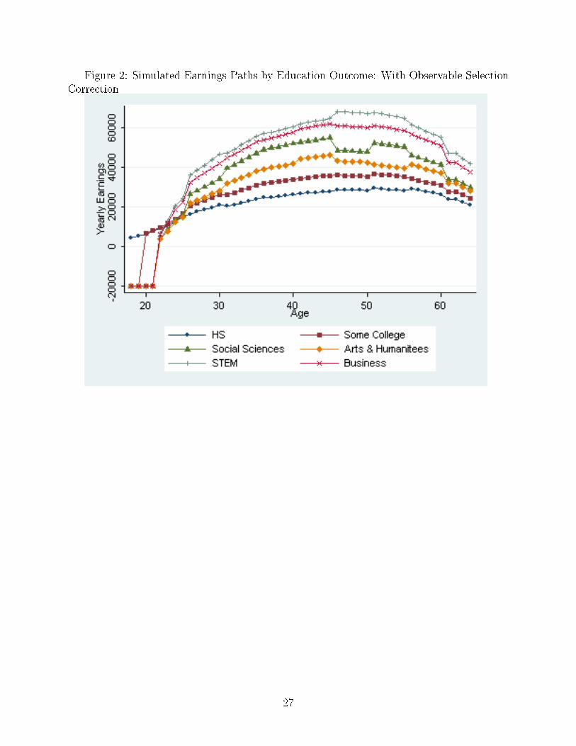
Figure 2: Simulated Earnings Paths by Education Outcome: With Observable SelectionCorrection
27

Figure 3:Cumulative Earnings Paths Minus Average Tuition by Education Outcome
28

Figure 4: Simulated Earnings Paths by Education Outcome: With Observable and Un-observable (Correlation=.50) Selection Corrections
29

Table 1: Summary StatisticsNLSY ACS
Black .121 .089Hispanic .054 .109High School .570 .387Some College .254 .366STEM .055 .072Business .056 .072Social Sciences .014 .025Arts and Humanities .013 .031Age 18-25 .189 .114Age 26-30 .213 .107Age 31-35 .182 .105Age 36-40 .127 .110Age 41-45 .1 25 .118Age 46-50 .122 .137Age 51-55 .008 .136Age 56-60 0 .133Age 61-64 0 .061AFQT 49.8Rotter 8.45Rosenberg 22.8Observations 51,377 475,896Each of the NLSY and ACS samples are comprised of men between theages of 18 and 64. Only individuals who have at least a high school
diploma but no postgraduate work are retained in the sample.Individuals who are currently enrolled in college or the military are
excluded.
30
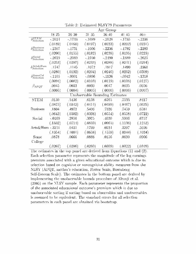
Table 2: Estimated NLSY79 ParametersAge Group
18-25 26-30 31-35 36-40 41-45 46+δSTEMSelection -.2024 -.1733 -.1689 -.2128 -.1735 -.2236
(.0189) (.0168) (.0197) (.0233) (.0202) (.0231)δBusinessSelection -.2307 -.1731 -.1666 -.2236 -.1792 -.2289
(.0200) (.0155) (.0182) (.0238) (.0195) (.0223)δSocialSelection -.2619 -.2089 -.1950 -.2490 -.1889 -.2625
(.0253) (.0207) (.0233) (.0288) (.0241) (.0294)δArts&HumSelection -.1747 -.1145 -.1072 -.1817 -.1490 -.2368
(.0280) (.0192) (.0204) (.0246) (.0262) (.0309)δSomeColSelection -.1105 -.0901 -.0896 -.1126 -.0942 -.1218
(.0094) (.0082) (.0103) (.0119) (.0108) (.0127)βAFQT .0045 .0033 .0030 .0047 .0035 .0056
(.0005) (.0004) (.0005) (.0006) (.0006) (.0007)Unobservable Bounding Estimates
STEM .0139 .5436 .6138 .6765 .7533 .8417(.0875) (.0342) (.0414) (.0499) (.0467) (.0635)
Business .1804 .4972 .5406 .7336 .7459 .6581(.0643) (.0302) (.0398) (.0554) (.0558) (.0722)
Social -.0169 .2856 .3975 .4030 .5906 .6757(.1332) (.0714) (.0859) (.0965) (.1136) (.1252)
Arts&Hum -.3251 .0431 .1799 .0234 .3297 .5026(.1354) (.1001) (.0658) (.1559) (.0944) (.1034)
SomeCollege
.0878 .0666 .0888 .0156 .0690 .0966
(.0267) (.0206) (.0260) (.0309) (.0322) (.0349)The estimates in the top panel are derived from Equations (1) and (2).Each selection parameter represents the magnitude of the log earningspremium associated with a given educational outcome which is due toselection based on cognitive or noncognitive ability measures from theNLSY (AFQT, mother's education, Rotter Scale, RosenbergSelf-Esteem Scale). The estimates in the bottom panel are derived byimplementing the unobservable bounds procedure of Altonji et al.(2005) on the NLSY sample. Each parameter represents the proportionof the associated educational outcome's premium which is due tounobservable sorting if sorting based on observables and unobservablesis assumed to be equivalent. The standard errors for all selectionparameters in each panel are obtained via bootstrap.
31

Table 3: Estimated ACS ParametersAge Group
18-25 26-30 31-35 36-40 41-45 46-50 51-55 56-60 61-64yHS 9.26 9.88 10.05 10.23 10.28 10.35 10.37 10.32 10.17
δSomeCol 0.118 0.251 0.293 0.277 0.277 0.256 0.246 0.191 .184δSTEM 0.507 0.818 0.895 0.875 0.876 0.894 0.837 0.769 .692δBusiness 0.450 0.738 0.846 0.846 0.850 0.796 0.771 0.684 .597δSocial 0.133 0.545 0.710 0.748 0.755 0.664 0.629 0.543 .467δArts&Hum -0.022 0.294 0.439 0.503 0.550 0.494 0.399 0.429 .324βAge 0.176 0.062 0.042 0.015 0.010 -0.004 -0.010 -0.026 -0.060σHS 1.10 0.997 0.986 0.927 0.958 0.920 0.926 0.941 1.01
σSomeCol 0.998 0.895 0.897 0.877 0.892 0.924 0.914 0.984 1.07σSTEM 0.966 0.729 0.697 0.748 0.802 0.801 0.849 0.938 1.16σBusiness 0.938 0.752 0.820 0.827 0.865 0.960 0.925 0.968 1.13σSocial 1.03 0.868 0.890 0.856 0.901 0.975 1.00 1.04 1.18σArts&Hum 1.03 0.905 0.905 0.971 0.983 0.991 1.03 1.03 1.20Each parameter is derived from Equation (5). The beta parametersrepresent the coe�cients associated with each age group andeducational outcome. The sigma parameters represent the standarddeviation of the low earnings residuals for each age group andeducational outcome.
32

Table 4: Average Simulated Lifetime Earnings
High School Some College STEM Business Social Sciences Arts/Humanities
No selection correction 1,513,893 2,021,148 3,706,155 3,573,792 3,240,067 2,664,811
(1) with observable correction 1,513,893 1,810,602 3,017,659 2,899,500 2,556,089 2,195,055
(2) with discount factor=.966 662,709 780,260 1,255,488 1,208,829 1,072,396 916,452
(3) with tuition deducted 662,709 740,940 1,168,544 1,122,496 990,295 831,429
% of (4) below HS mean .50 .387 .048 .080 .170 .299
Each value in the �rst four rows represents the median cumulative lifetime earnings as estimated from Equation (6)
associated with each educational outcome given the assumptions listed in the �rst column. The results are obtained
from a simulated sample of 100,000 individuals. All inputs to Equation (6) are obtained by estimating Equations
(1)-(5) on the sample of men described in the data section who had any positive earnings over the past year.
33
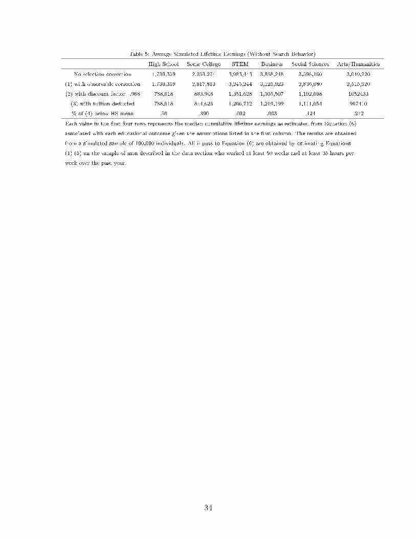
Table 5: Average Simulated Lifetime Earnings (Without Search Behavior)
High School Some College STEM Business Social Sciences Arts/Humanities
No selection correction 1,730,359 2,253,274 3,983,443 3,858,248 3,598,160 3,049,220
(1) with observable correction 1,730,359 2,017,813 3,245,244 3,125,923 2,836,080 2,515,920
(2) with discount factor=.966 788,618 883,946 1,351,628 1,305,507 1,192,608 1052433
(3) with tuition deducted 788,618 844,626 1,266,712 1,219,199 1,111,654 967410
% of (4) below HS mean .50 .390 .032 .063 .124 .242
Each value in the �rst four rows represents the median cumulative lifetime earnings as estimated from Equation (6)
associated with each educational outcome given the assumptions listed in the �rst column. The results are obtained
from a simulated sample of 100,000 individuals. All inputs to Equation (6) are obtained by estimating Equations
(1)-(5) on the sample of men described in the data section who worked at least 50 weeks and at least 35 hours per
week over the past year.
34
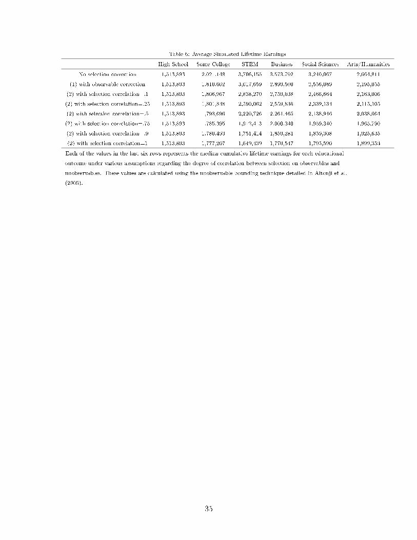
Table 6: Average Simulated Lifetime Earnings
High School Some College STEM Business Social Sciences Arts/Humanities
No selection correction 1,513,893 2,021,148 3,706,155 3,573,792 3,240,067 2,664,811
(1) with observable correction 1,513,893 1,810,602 3,017,659 2,899,500 2,556,089 2,195,055
(2) with selection correlation=.1 1,513,893 1,806,967 2,838,270 2,759,038 2,466,664 2,163,006
(2) with selection correlation=.25 1,513,893 1,801,848 2,590,062 2,559,836 2,339,134 2,115,105
(2) with selection correlation=.5 1,513,893 1,793,696 2,220,726 2,261,465 2,138,946 2,038,664
(2) with selection correlation=.75 1,513,893 1,785,395 1,912,413 2,000,340 1,959,340 1,965,790
(2) with selection correlation=.9 1,513,893 1,780,493 1,751,414 1,859,281 1,859,308 1,925,635
(2) with selection correlation=1 1,513,893 1,777,207 1,649,439 1,770,547 1,795,590 1,899,353
Each of the values in the last six rows represents the median cumulative lifetime earnings for each educational
outcome under various assumptions regarding the degree of correlation between selection on observables and
unobservables. These values are calculated using the unobservable bounding technique detailed in Altonji et al.
(2005).
35

Table 7: Average Simulated Lifetime Earnings (With Observable Selection Correction)
High School Some College STEM Business Social Sciences Arts/Humanities
Bottom ability quintile 1,345,539 1,493,596 2,336,281 2,259,346 2,000,010 1,767,486
Second ability quintile 1,477,684 1,639,564 2,527,325 2,477,975 2,179,365 1,874,196
Third ability quintile 1,641,838 1,810,818 2,714,336 2,666,429 2,446,121 2,023,277
Fourth ability quintile 1,823,478 1,985,081 3,000,551 2,908,076 2,694,806 2,228,259
Highest ability quintile 2,000,855 2,203,207 3,269,770 3,127,404 2,877,284 2,523,457
Each value represents the median cumulative lifetime earnings as estimated from Equation (6) associated with each
educational outcome given the assumptions listed in the �rst column. The results are obtained from a simulated
sample of 100,000 individuals. All inputs to Equation (6) are obtained by estimating Equations (1)-(5) on the
sample of men described in the data section who had any positive earnings over the past year.
36
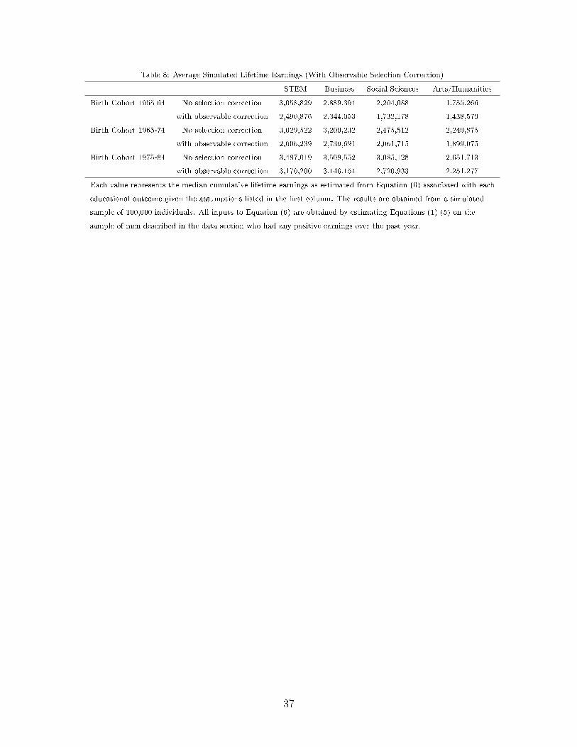
Table 8: Average Simulated Lifetime Earnings (With Observable Selection Correction)
STEM Business Social Sciences Arts/Humanities
Birth Cohort 1955-64 No selection correction 3,058,829 2,889,394 2,204,088 1,755,266
with observable correction 2,490,876 2,344,053 1,732,178 1,438,579
Birth Cohort 1965-74 No selection correction 3,029,522 3,209,232 2,475,512 2,249,875
with observable correction 2,606,239 2,739,691 2,061,715 1,899,075
Birth Cohort 1975-84 No selection correction 3,487,019 3,509,552 3,085,128 2,651,713
with observable correction 3,170,200 3,146,154 2,720,933 2,251,277
Each value represents the median cumulative lifetime earnings as estimated from Equation (6) associated with each
educational outcome given the assumptions listed in the �rst column. The results are obtained from a simulated
sample of 100,000 individuals. All inputs to Equation (6) are obtained by estimating Equations (1)-(5) on the
sample of men described in the data section who had any positive earnings over the past year.
37


