
The Merge/Purge Problem for Large Databases *
Abstract
Mauricio A. Hern&ndezt Salvatore J. Stolfo
{nrauricio, sal}@cs. columbi.a. edu
Department of Computer Science, Columbia University, New York, NY 10027
Many commercial organizations routinely gather large num-
bers of databases for various marketing and business analysis
functions. The task is to correlate information from different
databases by identifying distinct individuals that appear in
a number of different databases typically in an inconsistent
and oft en incorrect fashion. The problem we study here is
the task of merging data from multiple sources in as efficient
manner as possible, while maximizing the accuracy of the re-
sult. We call this the merge/purge problem. In this paper we
detail the sorted neighborhood method that is used by some
to solve merge/purge and present experimental results that
demonstrates this approach may work well in practice but at
great expense. An alternative method based upon clustering
is also presented with a comparative evaluation to the sorted
neighborhood method. We show a means of improving the
accuracy of the results based upon a multi-pass approach
that succeeds by computing the Transitive Closure over the
results of independent runs considering alternative primary
key attributes in each pass.
1 Introduction
In this paper we study a familiar instance of the se-
mantic integration problem[lO] or the instance identi-
fication problem[14], called the merge/purge problem.
Here we consider the problem over very large databases
of information that need to be processed as quickly, ef-
ficiently, and accurately as possible. For instance, one
month is a typical business cycle in certain direct mar-
keting operations. This means that sources of data need
to be identified, acquired, conditioned, and then corre-
“This work has been supported in part by the NYS Science
and Technology Foundation through the Center for Advanced
Technology in Telecommunicationsat PolytechnicU niversity,by
NSFunder grant IRI-94-13847, and by Citicorp.
tThisauthor’s work wassupported byan AT&T Cooperative
Research Program Fellowship.
Permission to copy without fee all or part of this material is9ranted provided that the copies are not made or distributed fordirect commercial advantaqe, the ACM copyright notice and thetitle of the publication and k date appear, and notice is giventhat copyin is by permission of the Association of Computing
fMachinery. o copy otherwise, or to republish, requiresa fee and/or specific permission.SIGMOD’95,San Jose, CA USAQ 1995 ACM 0-89791-731 -6/95/0005..$3.50
lated or merged within a small portion of a month in
order to prepare mailings and response analyses. For
example, it is common that many magazine subscrip-
tion databases are purchased for the specific purpose of
identifying characteristic interests of people for directed
marketing purposes. It is not uncommon for large busi-
nesses to acquire scores of databases each month, with
a total size of hundreds of millions to over a billion
records, that need to be analyzed within a few days.
Merge/purge is ubiquitous in modern commercial
organizations, and is typically solved today by expensive
mainframe computing solutions. Here we consider the
opportunity to solve merge/purge on low cost shared-
nothing multiprocessor architectures. Such approaches
are expected to grow in importance with the coming
age of very large network computing architectures
where many more distributed databases containing
information on a variety of topics will be generally
available for public and commercial scrutiny.
The merge/purge problem is closely related to a
multi-way join over a plurality of large database rela-
tions, The naive means of implementing joins is to com-
pute the Cartesian product, a quadratic time process,
and select relevant tuples. The obvious optimizations,
as well as parallel variants, for join computation are
well known: sort-merge and hash partitioning. These
strategies assume a total ordering over the domain of the
join attributes (an index is thus easily computable) or
a ‘(near perfect” hash function that provides the means
of inspecting small partitions of tuples when computing
the join. In the case we study here, we cannot assume
there exists a total ordering, nor a perfect hash distri-
bution that would lead to a completely accurate result,
meaning even slight errors in the data imply all possible
“matches” of common data about the same entity may
not be found. However, the techniques we study and
have implemented are based upon these two strategies
for fast execution, with the particular desire to improve
their accuracy.
The fundamental problem is that the data supplied
by various sources typically include identifiers or string
data, that are either different among different datasets
127

or simply erroneous due to a variety of reasons (includ-
ing typographical or transcription errors, or purpose-
ful fraudulent activity (aliases) in the case of names).
Hence, the equality of two values over the domain of
the common join attribute is not specified as a “sim-
ple” arithmetic predicate, but rather by a set of equa-
tional axioms that define equivalence, i.e., by an equa-
ttonai theory. Determining that two records from two
databases provide information about the same entity
can be highly complex. We use a rule-based knowledge
base to implement an equational theory, as detailed in
section 2.3.
Since we are dealing with large databases, we seek to
partition the database into partitions or clusters in such
a way that the potentially matching records are assigned
to the same cluster. (Here we use the term cluster in
line with the common terminology of statistical pattern
recognition. ) In this paper we first discuss a solution to
merge/purge in which sorting of the entire data-set is
used to bring the matching records close together in a
bounded neighborhood in a linear list. We then explore
the approach of partitioning the data into meaningful
clusters and then bringing the matching records on each
individual cluster close together by sorting. In the
second algorithm we need not compute an entire sort of
the full data-set, but rather a number of substantially
smaller, independent and concurrent sorts that can
be performed more efficiently on reduced datasets.
However, we demonstrate that, as one may expect,
neither of these basic approaches alone can guarantee
high accuracy without substantially decreasing the size
of the search neighborhood.
The contributions of this paper are as follows. We
detail a system we have implemented that performs a
generic merge/purge process that includes a declarative
rule language for specifying an equational theory mak-
ing it easier to experiment and modify the criteria for
equivalence. Alternative algorithms that were imple-
mented for the fundamental merge process are compar-
atively evaluated and demonstrate that no single pass
over the data using one particular scheme as a key per-
forms as well as computing the transitive closure over
several independent runs each using a different key for
ordering data. We show, for example, that multiple
passes followed by the computation of the closure consis-
tently dominates in accuracy for ordy a modest perfor-
mance penalty. Finally, we discuss the computational
costs of these alternative approaches and demonstrate
fully implemented parallel solutions to speed up the pro-
cess over a serial solution. The moral is simply that
several distinct “cheap” passes over the data produces
more accurate results than one “expensive” pass over
the data.
The rest of this paper is organized as follows. In the
next section, we will describe the specific details of the
mergefpurge problem we study, and two solutions based
upon sorted neighborhood searching and clustering.
Section 3 presents experimental results for our solution
method. Finally, parallel processing of these solutions
are briefly explored in section 4.
2 The Merge/Purge Problem
2.1 Problem description
Since we are faced with the task of merging very large
databases, we presume a pure quadratic time process
(i e., comparing each pair of records) is infeasible under
strict time constraints and limited capital budgets for
hardware. For pedagogical reasons we assume that each
record of the database represents information about
“employees” and thus contains fields for a social security
number, a name, and an address and other significant
information that may be utilized in determining equiv-
alence. Numerous errors in the contents of the records
are possible, and frequently encountered. For example,
names are routinely misspelled, parts are missing, salu-
tations are at times included as well as nicknames in
the same field. In addition, our employees may move
or marry thus increasing the variability of their asso-
ciated records. (Indeed, poor implementations of the
merge/purge task by commercial organizations typically
lead to several pieces of the same junk mail being mailed
at obviously greater expense to the same household, as
nearly everyone has experienced.)
There are two fundamental problems with performing
merge/purge. First, the size of the data sets involved
may be so large that only a relatively small portion of
the total available data can reside in main memory at
any point in time. Thus, the total database primarily
resides on external store and any algorithm employed
must be efficient, requiring as few passes over the data
set as possible.
Second, the incoming new data is corrupted, either
purposefully or accidentally, and thus the identification
of matching data requires complex tests to identify
matching data. The inference that two data items
represent the same domain entity may depend upon
considerable statistical, logical and empirical knowledge
of the task domain. “Faulty” inferences can be in some
cases worse than missing some matching data. The
“accuracy” of the result (maximizing the number of
correct matches while minimizing the number of false
positives) is therefore of paramount importance. It is
common that much of the engineering of a merge/purge
process is devoted to experiment and comparative
evaluation of the accuracy of the overall process, and
in particular alternative criteria for matching records.
2.2 The sorted neighborhood method
We consider two approaches to obtaining efficient
execution of any solution: partition the data to reduce
128
the combinatorics of matching large data sets, and
utilize parallel processing. We require a means of
effectively partitioning the data set in such a way as
to restrict our attention to a number of small sets of
candidates for matching. Consequently, we can process
the candidate sets in parallel. Furthermore, if the
candidate sets can be restricted to a very small subset
of the data, quadratic time algorithms applied to each
candidate set may indeed be feasible in the allotted time
frame for processing, leading to perhaps better accuracy
of the merge task.
One obvious method for bringing matching records
close together is sorting the records over the most
important discriminating key attribute of the data.
After the sort, the comparison of records is then
restricted to a small neighborhood within the sorted list.
We call this method the sorted neighborhood method.
The effectiveness of this approach is based on the quality
of the chosen keys used in the sort. Poorly chosen keys
will result in a poor quality merge, i.e., data that should
be merged will be spread out far apart after the sort and
hence will not be discovered. Keys should be chosen so
that the attributes with the most discriminatory power
should be the principal field inspected during the sort.
This means that similar and matching records should
have nearly equal key values. However, since we assume
the data is corrupted and keys are extracted directly
from the data, then the keys will also be corrupted.
Thus, we may expect that a substantial number of
matching records will not be caught. Our experimental
results, presented in section 3, demonstrate this to be
the case.
Given a collection of two or more databases, we first
concatenate them into one sequential list of N records
(after conditioning the records) and then apply the
sorted neighborhood method. The sorted neighborhood
method for solving the merge/purge problem can be
summarized in three phases:
1
2<
3.
Create Keys : Compute a key for each record in
the list by extracting relevant fields or portions of
fields.
Sort Data : Sort the records in the data list using
the key of step 1.
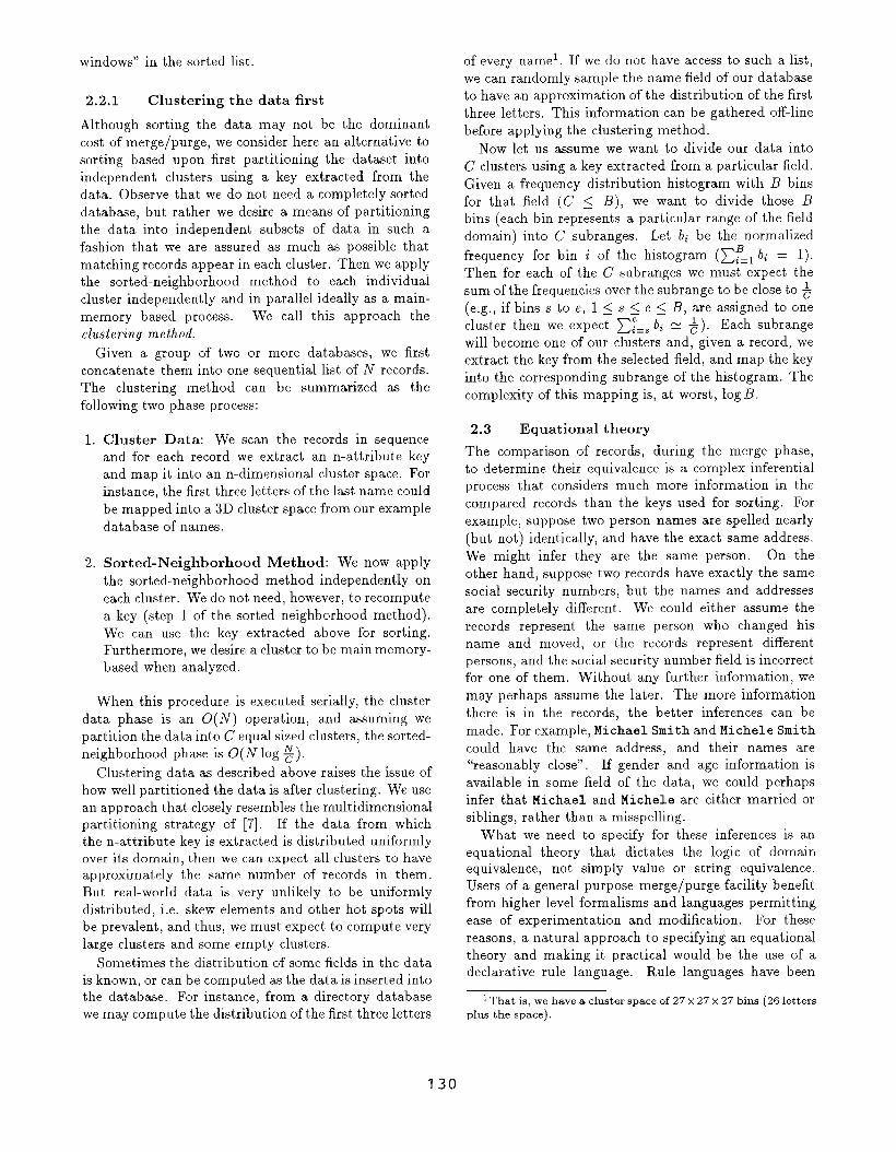
Merge : Move a fixed size window through the
sequential list of records limiting the comparisons for
matching records to those records in the window. If
the size of the window is w records, then every new
record entering the window is compared with the
previous w – 1 records to find “matching” records.
The first record in the window slides out of the
window (see figure 1).
Sorting and then merging within a window is the
essential approach of a Sort Merge Band Join as
Current windowof records
.
.●
❛❞
r~...w
11w. .. . . . ..
.,
------ ---
.
.
)Next windowof recordx
J
Figure 1: Window Scan during the Merge Phase
described by DeWitt [5]. As described in that paper, the
sort and merge phase can be combined in one pass. The
differences from this previous work and ours in the use of
a complex function (the equational theory) to determine
if records under consideration ‘(match”, and our concern
for the accuracy of the computed result since matching
records may not appear within a common “band”.
In [9], we describe the sorted-neighborhood method as a
generalization of band joins and provide an alternative
algorithm for the sorted-neighborhood method based
on the dupltcate ehmtnatton algorithm described in [3].
This duplicate elimination algorithms takes advantage
of the fact that ‘(matching” records will come together
during different phases of the Sort phase. Due to space
limitations, we will not describe this alternative solution
here.
When this procedure is executed serially as a main-
memory based process, the create keys phase is an O(N)
operation, the sorting phase is O(N log N), and the
merging phase is O(WN), where N is the number of
records in the database. Thus, the total time complexity
of this method is O(Nlog N) if w < [log Nl, O(WN)
otherwise. However, the constants in the equations
differ greatly. It could be relatively expensive to extract
relevant key values from a record during the create
key phase. Sorting requires a few machine instructions
to compare the keys. The merge phase requires the
application of a potentially large number of rules to
compare two records, and thus has the potential for the
largest constant factor.
Note, however, that it may be the case, that for very
large databases the dominant cost will be disk 1/0,
i.e., the number of passes over the data set. In this
case, at least three passes would be needed, one pass
for conditioning the data and preparing keys, at least
a second pass, likely more, for a high speed sort like,
for example, the AlphaSort [13], and a final pass for
window processing and application of the rule program
for each record entering the sliding window. Depending
upon the complexity of the rule program, the last pass
may indeed be the dominant cost. Later we consider the
means of improving this phase by processing “parallel
129
windows” in the sorted list.
2.2.1 Clustering the data first
Although sorting the data may not be the dominant
cost of merge/purge, we consider here an alternative to
sorting based upon first partitioning the dataset into
independent clusters using a key extracted from the
data. Observe that we do not need a completely sorted
database, but rather we desire a means of partitioning
the data into independent subsets of data in such a
fashion that we are assured as much as possible that
matching records appear in each cluster. Then we apply
the sorted-neighborhood method to each individual
cluster independently and in parallel ideally as a main-
memory based process. We call this approach the
clustering method.
Given a group of two or more databases, we first
concatenate them into one sequential list of N records.
The clustering method can be summarized as the
following two phase process:
1.
2.
Cluster Data: We scan the records in sequence
and for each record we extract an n-attribute key
and map it into an n-dimensional cluster space. For
instance, the first three letters of the last name could
be mapped into a 3D cluster space from our example
database of names.
Sorted-Neighborhood Method: We now apply
the sorted-neighborhood method independently on
each cluster. We do not need, however, to recompute
a key (step 1 of the sorted neighborhood method).
We can use the key extracted above for sorting.
Furthermore, we desire a cluster to be main memory-
based when analyzed.
When this procedure is executed serially, the cluster
data phase is an O(N) operation, and assuming we
partition the data into C equal sized clusters, the sorted-
neighborhood phase is O(N log ~).
Clustering data as described above raises the issue of
how well partitioned the data is after clustering. We use
an approach that closely resembles the multidimensional
partitioning strategy of [7]. If the data from which
the n-attribute key is extracted is distributed uniformly
over its domain, then we can expect all clusters to have
approximately the same number of records in them.
But real-world data is very unlikely to be uniformly
distributed, i.e. skew elements and other hot spots will
be prevalent, and thus, we must expect to compute very
large clusters and some empty clusters.
Sometimes the distribution of some fields in the data
is known, or can be computed as the data is inserted into
the database. For instance, from a directory database
we may compute the distribution of the first three letters
of every namel. If we do not have access to such a list,
we can randomly sample the name field of our database
to have an approximation of the distribution of the first
three letters. This information can be gathered off-line
before applying the clustering method.
Now let us assume we want to divide our data into
C clusters using a key extracted from a particular field.
Given a frequency distribution histogram with B bins
for that field (C < B), we want to divide those B
bins (each bin represents a particular range of the field
domain) into C subranges. Let bi be the normalized
frequency for bin i of the histogram (~~=1 bi = 1).
Then for each of the C subranges we must expect the
sum of the frequencies over the subrange to be close to ~
(e.g., if bins s to e, 1< s < e < B, are assigned to one
cluster then we expect ~~=~ bi = &). Each subrange
will become one of our clusters and, given a record, we
extract the key from the selected field, and map the key
into the corresponding subrange of the histogram. The
complexity of this mapping is, at worst, log B.
2.3 Equational theory
The comparison of records, during the merge phase,
to determine their equivalence is a complex inferential
process that considers much more information in the
compared records than the keys used for sorting. For
examplej suppose two person names are spelled nearly
(but not) identically, and have the exact same address.
We might infer they are the same person. On the
other hand, suppose two records have exactly the same
social security numbers, but the names and addresses
are completely different. We could either assume the
records represent the same person who changed his
name and moved, or the records represent different
persons, and the social security number field is incorrect
for one of them. Without any further information, we
may perhaps assume the later. The more information
there is in the records, the better inferences can be
made. For example, Michael Smith and Michele Smith
could have the same address, and their names are
“reasonably close”. If gender and age information is
available in some field of the data, we could perhaps
infer that Michael and Michele are either married or
siblings, rather than a misspelling.
What we need to specify for these inferences is an
equational theory that dictates the logic of domain
equivalence, not simply value or string equivalence.
Users of a general purpose merge/purge facility benefit
from higher level formalisms and languages permitting
ease of experimentation and modification. For these
reasons, a natural approach to specifying an equational
theory and making it practical would be the use of a
declarative rule language. Rule languages have been
1That is, we have a cluster space of 27 x 27 x 27 bins (26 letters
plus the space).
130
effectively used in a wide range of applications requiring
inference over large data sets. Much research has
been conducted to provide efficient means for their
compilation and evaluation, and this technology can
be exploited here for purposes of solving merge/purge
efficiently.
As an example, here is a simplified rule in English that
exemplifies one axiom of our equational theory relevant
to merge/purge applied to our idealized employee
database:
Given two records , rl and r2
IF the last name of rl equals the last name of r2 ,
AND the first names differ slightly,
AED the address of rl equals the address of r2
THEE
rl is equivalent. to r2.
The implementation of “differ slightly” specified
here in English is based upon the computation of a
distance function applied to the first name fields of two
records, and the comparison of its results to a threshold
to capture obvious typographical errors that may occur
in the data. The selection of a distance function
and a proper threshold is also a knowledge intensive
activity that demands experimental evaluation. An
improperly chosen threshold will lead to either an
increase in the number of falsely matched records or
to a decrease in the number of matching records that
should be merged. A number of alternative distance
functions for typographical mistakes were implemented
and tested in the experiments reported below including
distances based upon edit dwtance, phonetic distance
and “typewriter” distance. The results displayed in
section 3 are based upon edit distance computation
since the outcome of the program did not vary much
among the different distance functions for the particular
databases used in our study.
For the purpose of experimental study, we wrote an
OPS5[6] rule program consisting of 26 rules for this
particular domain of employee records and was tested
repeatedly over relatively small databases of records.
Once we were satisfied with the performance of our
rules, distance functions, and thresholds, we recoded
the rules directly in C to obtain speed-up over the 0PS5
implementation2.
It is important to note that the essence of the ap-
proach proposed here permits a wide range of “equa-
tional theories” on various data types. We chose to
use string data in this study (e.g., names, addresses)
for pedagogical reasons (after all everyone gets “faulty”
2At the time the system was built, the public dOmain Ops 5
compiler was simply t 00 slow for our experimental purposes.
Another 0PS5C compiler [12] was not available to us in timefor these studies. The 0PS5C compiler produces code thatis reportedly many times faster than previous compilers. We
captured thk speed advantage for our study hereby hand recoding
our rules in C.
junk mail). We could equally as well demonstrate the
concepts using alternative databases of different typed
objects and correspondingly different rule sets.
2.4 Computing the transitive closure over
the results of independent runs
The effectiveness of the sorted neighborhood method
highly depends on the key selected to sort the records. A
key is defined to be a sequence of a subset of attributes,
or substrings within the attributes, chosen from the
record. For example, we may choose a key as the last
name of the employee record, followed by the first non
blank character of the first name sub-field followed by
the first six digits of the social security field, and so
forth.
In general, no single key will be sufficient to catch all
matching records. Attributes that appear first in the
key have a higher priority than those appearing after
them. If the error in a record occurs in the particular
field or portion of the field that is the most important
part of the key, there may be little chance a record will
end up close to a matching record after sorting. For
instance, if an employee has two records in the database,
one with social security number 193456782 and another
with social security number 913456782 (the first two
numbers were transposed), and if the social security
number is used as the principal field of the key, then
it is very unlikely both records will fall under the same
window, i.e. the two records with transposed social
security numbers will be far apart in the sorted list and
hence they may not be merged. As we will show in the
next section, the number of matching records missed
by one run of the sorted neighborhood method can be
large.
To increase the number of similar records merged, two
options were explored, The first is simply widening the
scanning window size by increasing w. Clearly this in-
creases the computational complexity, and, as discussed
in the next section, does not increase dramatically the
number of similar records merged in the test cases we
ran until w becomes excessively large.
The alternative strategy we implemented is to execute
several independent runs of the sorted neighborhood
method, each time using a different key and a relative~y
small window. We call this strategy the multi-pass
approach. For instance, in one run, we use the address
as the principal part of the key while in another run we
use the last name as the principal part of the key. Each
independent run will produce a set of pairs of records
which can be merged. We then apply the transitive
closure to those pairs of records. The results will be a
union of all pairs discovered by all independent runs,
with no duplicates, plus all those pairs that can be
inferred by transitivity of equality.
The reason this approach works for the test cases
explored here has much to do with the nature of the
131
errors in the data. Transposing the first two digits of
the social security number leads to unmergeable records
as we noted. However, in such records, the variability
or error appearing in another field of the records may
indeed not be so large. Therefore, although the social
security numbers in two records are grossly in error,
the name fields may not be. Hence, first sorting on
the name fields as the primary key will bring these two
records closer together lessening the negative effects of
a gross error in the social security field.
It is clear that the utility of this approach is therefore
driven by the nature and occurrences of the errors
appearing in the data. Once again, the choice of
keys for sorting, their order, and the extraction of
relevant information from a key field is a knowledge
intensive activity that must be explored prior to running
a merge/purge process.
In the next section we will show how the multi-pass
approach can drastically improve the accuracy of the
results of only one run of the sorted neighborhood
method with varying large windows. Of particular
interest is the observation that only a small search
window was needed for the multi-pass approach to
obtain high accuracy while no individual run with a
single key for sorting produced comparable accuracy
results with a large window (other than
approaching the size of the full database).
were found consistently over a variety
databases with variable errors introduced
3 Experimental Results
3.1 Generating the databases
window sizes
These results
of generated
in all fields.
All databases used to test the sorted neighborhood
method and the clustering method were generated
automatically by a database generator that allow us to
perform controlled studies and to establish the accuracy
of the solution method. This database generator
provides a large number of parameters including, the
size of the database, the percentage of duplicate records
in the database, and the amount of error to be
introduced in the duplicated records in any of the
attribute fields. Each record generated consists of the
following fields, some of which can be empty: social
security number, first name, initial, last name, address,
apartment, city, state, and zip code. The names were
chomn randomly from a list of 6300(1 real names. The
cities, states, and zip codes (all from the U.S .A) come
from publicly available lists.
The errors introduced in the duplicate records range
from small typographical changes, to complete change
of last names and addresses. When setting the pa-
rameters for the kind of typographical errors, we used
known frequencies from studies in spelling correction
algorithms [11]. For this study, the generator selected
from 10% to 50% of the generated records for duplica-
tion with errors, where the error was controlled accord-
ing to published statistics found for common real world
datasets.
3.2 Pre-processing the database
Pre-processing and conditioning the records in the
database prior to the merge/purge operation might
increase the chance of finding two duplicate records.
For example, names like Joseph and Gius eppe match
in only three characters, but are the same name in two
different languages, English and Italian. A nicknames
database or name equivalence database is used to
assign a common name to records containing identified
nicknames.
Since misspellings are introduced by the database
generator, we explored the possibility of improving
the results by running a spelling correction program
over some fields. Spelling correction algorithms have
received a large amount of attention for decades [1 I].
Most of the spelling correction algorithms we considered
use a corpus of correctly spelled words from which the
correct spelling is selected. Since we only have a corpus
for the names of the cities in the U.S.A. (18670 different
names), we only attempted correcting the spelling of the
city field. We chose the algorithm described by Bickel
in [2] for its simplicity and speed. Although not shown
in the results presented in this paper, the use of spell
corrector over the city field improved the percent of
correctly found duplicated records by only 1.570-2 .OYO.
Most of the effort in matching resides in the equational
theory rule base.
3.3 Initial results on accuracy
The purpose of this first experiment was to determine
baseline accuracy of the sorted-neighborhood method.
We ran three independent runs of the sorted neighbor-
hood method over each database, and used a different
key during the sorting phase of each independent run.
On the first run the last name was the principal field
of the key. On the second run, the first name was the
principal field, while in the last run, the street address
was the principal field. Our selection of the attribute
ordering of the keys was purely arbitrary. We could
have used the social-security number instead of, say,
the street address. We assume all fields are noisy (and
under the control of our data generator to be made so)
and therefore it does not matter what field ordering we
select for purposes of this study.
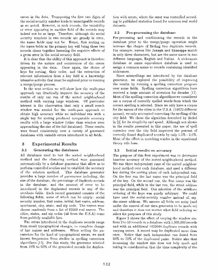
Figure 2 shows the effect of varying the window size
from 2 to 50 records in a database with 1,000,000 records
and with an additional 1423644 duplicate records with
varying errors. A record may be duplicated more than
once. Notice that each independent run found from
50’%0 to 70~o of the duplicated pairs. Notice also that
increasing the window size does not help much and
taking in consideration that the time complexity of the
132
Sorted-Neighborhood Method (1 M records + 423644 duphcates)
‘:-
170
60 -
50 -,s
d:
400 10 20 30 40 50 60
Window Size (records)
Sorted-Neighborhood Method (1 M records + 423644 duplicates)02
Key #1 (Last Name) +Key #2 (First Name) -+--
Key #3 (St Addr,) -SI-Multi-pses over 3 keys -&-
/.0,15 ./.
/
‘; “e-
0 10 20 30 40 50Window Size (records)
(a) Percent of correctly detected duplicated pairs (b) Percent of incorrectly detected duplicated pairs
Figure 2: Accuracy results for a 1,000,000 records database
procedure goes up as the window size increases, it is
obviously fruitless at some point to use a large window.
The line marked as Multtpass over 3 keys in figure 2
shows our results when the program computes the
transitive closure over the pairs found by the three
independent runs. The percent of duplicates found goes
up to almost 90’ZO. A manual inspection of those records
not found as equivalent revealed that most of them are
pairs that would be hard for a human to identify without
further information.
As mentioned above, our equational theory is not
completely trustworthy. It can mark two records as
similar when they are not the same real-world entity
(false-positives). Figure 2 shows the percent of those
records incorrectly marked as duplicates as a function
of the window size. The percent of false positives is
almost insignificant for each independent run and grows
slowly as the window size increases. The percent of
false positives after the transitive closure is also very
small, but grows faster than each individual run alone.
This suggests that the transitive-closure may not be as
accurate if the window size of each constituent pass is
very large!
The number of independent runs needed to obtain
good results with the computation of the transitive
closure depends on how corrupt the data is and the
keys selected. The more corrupted the data, more runs
might be needed to capture the matching records. The
transitive closure, however, is executed on pairs of tuple
id’s, each at most 30 bits, and fast solutions to compute
transitive closure exist [1], From observing real world
scenarios, the size of the data set over which the closure
is computed is at least one order of magnitude smaller
than the
does not
corresponding database
contribute a large cost.
of rec-ords, and thus
But note we pay a
heavy price due to the number of sorts or clusterings
of the original large data set. We address this issue in
section 4.
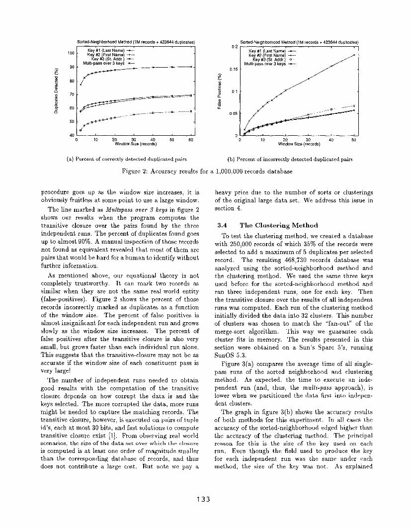
3.4 The Clustering Method
To test the clustering method, we created a database
with 250,000 records of which 35’% of the records were
selected to add a maximum of 5 duplicates per selected
record. The resulting 468,730 records database was
analyzed using the sorted-neighborhood method and
the clustering method. We used the same three keys
used before for the sorted-neighborhood method and
ran three independent runs, one for each key. Then
the transitive closure over the results of all independent
runs was computed. Each run of the clustering method
initially divided the data into 32 clusters. This number
of clusters was chosen to match the “fan-out” of the
merge-sort algorithm. This way we guarantee each
cluster fits in memory. The results presented in this
section were obtained on a Sun’s Spare 5 ‘s, running
SunOS 5.3.
Figure 3(a) compares the average time of all single-
pass runs of the sorted neighborhood and clustering
method. As expected, the time to execute an inde-
pendent run (and, thus, the multi-pass approach), is
lower when we partitioned the data first into indepen-
dent clusters.
The graph in figure 3(b) shows the accuracy results
of both methods for this experiment. In all cases the
accuracy of the sorted-neighborhood edged higher than
the accuracy of the clustering method. The principal
reason for this is the size of the key used on each
run. Even though the field used to produce the key
for each independent run was the same under each
method, the size of the key was not. As explained
133
3500 - Average single-pass time, SNM *Average single-pass time, Clustering -t-
Total mulb-pass !Ime, SNM %3000 Total multl-pass time, Clustering -x-
2500 -
2000 ~
./--’
1500 -
‘:+--5OL I
2 34 6 78Wl~dow size (records)
9 10
100, I
90 ... — .. .. —----+ . . . . . . . . . . . . 4 (
80I i
70
-..e.._../.. &””-””””_””””_”-”””_””””_”SNM, Key 1 +
50SNM, Key 2 +
,--- SNM, Key 3 %=
[ “-’ SNM, Multi-pass w ALL Keys ++-Clustermg, Key 1 -4––
40 - Clustering, Key 2 -+=Clustering, Key 3 -B–
Clustering, Mutti-pass w ALL Keys -K-–30
2 4 6 8 10Window SIZEI(records)
(a) Average Total Times (b) Accuracy of Results
Figure 3: Clustering Method vs. Sorted Neighborhood Method on 1 processor
in section 2.2.1, the clustering method uses the fixed-
sized key extracted during its clustering phase to later
sort each cluster independently. On the other hand, the
sorted-neighborhood method used the complete length
of the strings in the key field, making the size of the
key used variable. Records that should be merged are
expected to end closer together in a sorted list the larger
the size of the key used. Since, for the case of this
experiment, the average size of the key used by the
sorted-neighborhood method is larger that the one used
by the clustering method, we must expect the sorted-
neighborhood method to produce more accurate results.
Figure 3(b) also shows how the accuracy improves after
the multi-pass approach is applied to the independent
runs. As we saw in the previous section, when we
applied the closure to all pairs found to be similar with
the three independent runs, the accuracy jumped to over
90% for w >4.
3.5 Analysis
The natural question to pose is when is the muk
pass approach superior to the single-pass case? The
answer to this question lies in the complexity of the two
approaches for a fixed accuracy rate (for the moment we
consider the percentage of correctly found matches).
Here we consider this question in the context of a
main-memory based sequential process, The reason
being that, as we shall see, clustering provides the
opportunity to reduce the problem of sorting the
entire disk-resident database to a sequence of smaller,
main-memory based analysis tasks. The serial time
complexity of the multz-pass (rep) approach (with r
passes) is given by the time to create the keys, the time
to sort r times, the time to window scan r times (of
window size w) plus the time to compute the transitive
closure. In our experiments, the creation of the keys
was integrated into the sorting phase. Therefore, we
treat both phases as one in this analysis. Under the
simplifying assumption that all data is memory resident
(i.e., we are not 1/0 bound),
TmP = c, O,trN Iog N + cWscanrwN + Tclm,
where r is the number of passes and TCl~p is the time for
the transitive closure. The constants depict the costs for
comparison only and are related as cu~c~~ = ac~oTi, ,
where a > 1. From analyzing our experimental
program, the window scanning phase contributes a
constant, cv~can, which is at least a = 6 times as
large as the comparisons performed in sorting. We
replace the constants in terms of the single constant
c. The complexity of the closure is directly related to
the accuracy rate of each pass and depends upon the
duplication in the database. However, we assume the
time to compute the transitive closure on a database
that is orders of magnitude smaller than the input
database to be less than the time to scan the input
database once (i.e. it contributes a factor of cC(N < N).
Therefore,
T~P = crN log N + ~crwN + Tcim,,
for a window size of w. The complexity of the single pass
(sp) sorted-neighborhood approach is similarly given by:
T~P = C~ log~ + CMCW’N + TGr,P
for a window size of W.
For a fixed accuracy rate, the question is then for
what value of W of the single pass sorted-neighborhood
method does the multz-pass approach perform better in
time, i.e. , when 1s T~P > T~P. Solving this inequality,
we have:
w>r—1— log N + rw + & (TCl~P – T./,P)
a
134
1000/’
Key 1 (last name) -Key 2 (first name) -+-
Key 3 (street addr) *---800 - Multl-pass w, all keys x--- / L
600
400 -
200 ~
56,5 ~-,y~,,, ,,,,,,,,Of
2 10 52 100 1000Window Size (W)
(a) Time for each single-pass runs and the multi-pass run
55 I d
2 10 52 100 1000 10000Window Size (W)
(b) Accuracy of each single-pass runs and the multi-pass
run
Figure4: Time and Accuracy fora Memory-based Database (13751 records)
w>r—1—log N+rw+
r—1~TCl,P + —
a CY:NTC1mp
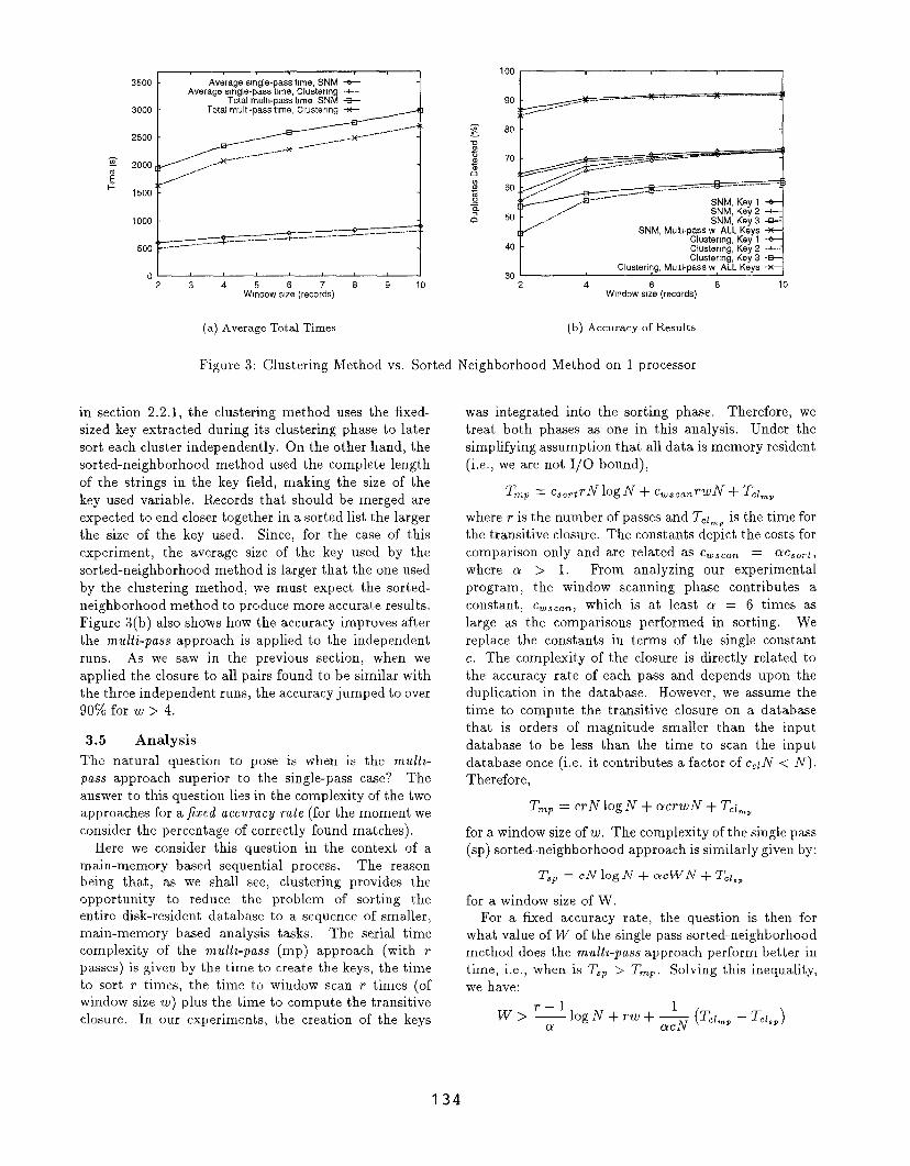
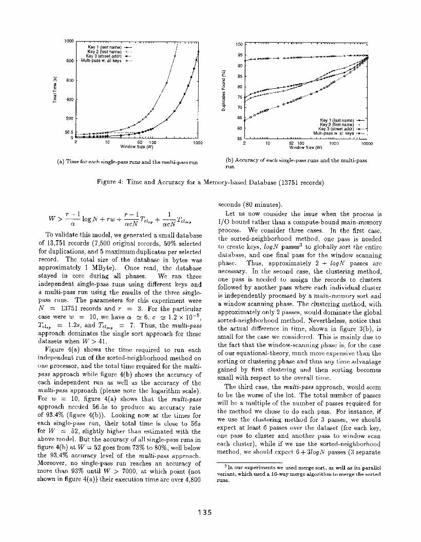
To validate this model, we generated a small database
of 13,751 records (7,500 original records, 5070 selected
for duplications, and 5 maximum duplicates per selected
record. The total size of the database in bytes was
approximately 1 MByte). once read, the database
stayed in core during all phases. We ran three
independent single-pass runs using different keys and
a multi-pass run using the results of the three single-
pass runs. The parameters for this experiment were
N = 13751 records and r = 3. For the particular
case were w = 10, we have a ~ 6, c N 1.2 x 10⁻⁵,
TC/,, = 1.2s, and T.lm, = 7. Thus, the multi-pass
approach dominates the single sort approach for these
datasets when W >41.
Figure 4(a) shows the time required to run each
independent run of the sorted-neighborhood method on
one processor, and the total time required for the muiti-
pass approach while figure 4(b) shows the accuracy of
each independent run as well as the accuracy of the
multi-pass approach (please note the logarithm scale).
For w = 10, figure 4(a) shows that the multi-pass
approach needed 56.5s to produce an accuracy rate
of 93.470 (figure 4(b)). Looking now at the times for
each single-pass run, their total time is close to 56s
for W = 52, slightly higher than estimated with the
above model. But the accuracy of all single-pass runs in
figure 4(b) at W = 52 goes from 73% to 80%, well below
the 93 .4~o accuracy level of the multi-pass approach.
Moreover, no single-pass run reaches an accuracy of
more than 9370 until W > 7000, at which point (not
shown in figure 4(a)) their execution time are over 4,800
seconds (80 minutes).
Let us now consider the issue when the process is
1/0 bound rather than a compute-bound main-memory
process. We consider three cases. In the first case,
the sorted-neighborhood method, one pass is needed
to create keys, iogN passes3 to globally sort the entire
database, and one final pass for the window scanning
phase. Thus, approximately 2 + iogN passes are
necessary. In the second case, the clustering method,
one pass is needed to assign the records to clusters
followed by another pass where each individual cluster
is independently processed by a main-memory sort and
a window scanning phase. The clustering method, with
approximately only 2 passes, would dominate the global
sorted-neighborhood method. Nevertheless, notice that
the actual difference in time, shown in figure 3(b), is
small for the case we considered. This is mainly due to
the fact that the window-scanning phase is, for the case
of our equational-theory, much more expensive than the
sorting or clustering phase and thus any time advantage
gained by first clustering and then sorting becomes
small with respect to the overall time.
The third case, the multi-pass approach, would seem
to be the worse of the lot. The total number of passes
will be a multiple of the number of passes required for
the method we chose to do each pass. For instance, if
we use the clustering method for 3 passes, we should
expect at least 6 passes over the dataset (for each key,
one pass to cluster and another pass to window scan
each cluster), while if we use the sorted-neighborhood
method, we should expect 6 + 310gN passes (3 separate
3 ~ ~ur ~XPeriments We used merge sort, as we~ as its Parallel
variant, which used a 16-way merge algorithm to merge the sorted
runs.
135
sorts). Clearly then the multt-pass approach would be
the worst performer in time over the less expensive
clustering method. Figure 3 shows this increase in time.
However, notice the large difference in accuracy between
the multi-pass and single-pass approaches in figure 3(a).
Clearly the multt-pass approach has a larger accuracy
than any of the two single-pass approaches. Thus, in a
serial environment, the user must weigh this trade-off
between execution time and accuracy.
In the next section we explore parallel variants of the
three basic techniques discussed here to show that with
suitable parallel hardware, we can speed-up the multi-
pass approach to a level comparable to the time to do
a single-pass approach, but with a very high accuracy,
i.e. a few small windows ultimately wins.
4 Parallel implementation
With the use of a centralized parallel or distributed
shared-nothing multiprocessor computer we seek to
achieve a linear speedup over a serial computer. Here
we briefly sketch the means to achieve this goal.
4.1 Single and Multi-pass sorted
neighborhood method
The parallel implementation of the sorted-neighborhood
method is as follows. Let N be the number of records
in the database, P be the number of processors in
our multiprocessor environment, and w be the size (in
number of records) of the merge phase window.
For the sort phase, a coordinator processor (CP)
fragments the input database in a round-robin fashion
among all P sites. Each site then sorts its local fragment
in parallel. Then the CP does a P-way join, reading a
block at a time (as needed) from each of the P sites.
Conceptually, for the merge phase, we should start
by partitioning the input database into P fragments
and assign each fragment to a different processor. The
fragment assigned to processor i should replicate the last
w — 1 records from the fragment assigned to site i — 1,
for 1< i ~ P. Similarly, for 1 ~ i < P, the fragment at
site i should replicate the first w — 1 records from the
fragment at site i+ 1. These small “bands” of replicated
records are needed to make the fragmentation of the
database invisible when the window scanning process is
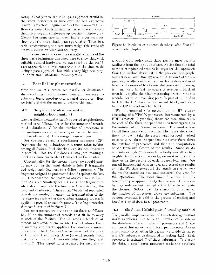
applied in parallel to each fragment. This fragmentationstrategy is depicted in figure 5.
For concreteness, we divide the database as follows.
Let &f be the number of records that fit in memory
at each of the P sites. The CP reads a block of Azf
records and sends them to site 1 which stores them
in memory and starts applying the window scanning
procedure. The CP stores the last w – 1 of the block
sent to site 1 and reads M — (w — 1) records from
disk, for a total of M records which are then sent
to site 2. This algorithm is repeated for each site in
N recordsk x
I k--M+ I1 1
. ..1t , (
PSite1 P Site 3 J ““” &
Site ‘2 S,te 4 Site (P-1)
Figure 5: Partition of a sorted database with ‘(bards”
of replicated tuples.
a round-robin order until there are no more records
available from the input database. Notice that the total
number of replicated records is larger for this approach
than the method described in the previous paragraph.
Nevertheless, with this approach the amount of time a
processor is idle is reduced, and each site does not need
to write the received blocks into disk since its processing
is in memory. In fact, as each site receives a block of
records, it applies the window scanning procedure to the
records, sends the resulting pairs (a pair of tuple id’s)
back to the CP, discards the current block, and waits
for the CP to send another block.
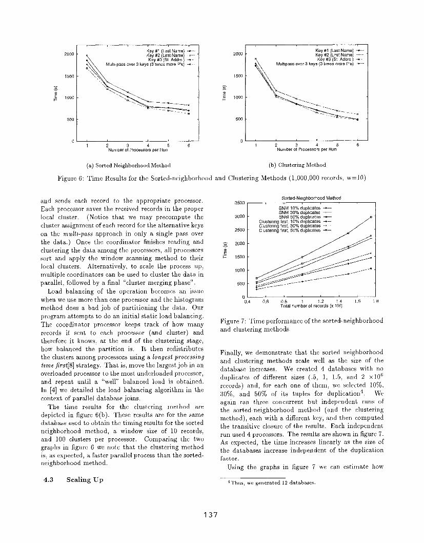
We implemented this method on an HP cluster
consisting of 8 HP9000 processors interconnected by a
FDDI network. Figure 6(a) shows the total time taken
for each of the three independent runs from figure 2 as
the number of processors increases. The window size
for all these runs was 10 records. The figure also shows
the time it will take the sorted-neighborhood method
to execute all three independent runs over three times
the number of processors and then the computation
of the transitive closure of the results. Since we do
not have enough processors to actually run all sorted-
neighborhood runs concurrently, we must estimate this
time using the results of each independent run. We
ran all independent runs in turn and stored the results
on disk. We then computed the transitive closure over
the results stored on disk and measured the time for
this operation. The total time, if we run all runs
concurrently, is approximately the maximum time taken
by any independent run plus the time to compute
the closure. Notice that the speed-ups obtained as
the number of processors grows are sublinear. The
obvious overhead is paid in the process of reading and
broadcasting of data to all processors.
4.2 Single and Multi-pass clustering method
The parallel implementation of the clustering method
works as follows. Let N be the number of records in
the database, P the number of processors and C the
number of clusters we want to form per processor. Given
a frequency distribution histogram, we divide its range
into C’P subranges as described in section 2.2.1. Each
processor is assigned C of those subranges. To cluster
the data, a coordinator processor reads the database
136
2000
1500
@
?1= 1000
500
0
,-—,—r –.
Key #1 (Last Name) +--Key #2 (Lwst Name) +--- -Key #3 (St Addrs ) ..@
Multi-pass over 3 keys (3 times more P’s) +---
-.,
---—.!+—..= *
..
i
1 2 3 4 5 6Number of Processors per Run
(a) Sorted Neighborhood M,thod
2000
1500
~:F= 1000
500
0
Key #1 Last Name) +-
[’Key #2 Lirst Name) -+---x Key #3 (St Addrs ) *+ Multlpass over 3 keys (3 t!mes more P’s) —+—
1 2 3 4 5 6Number of Processors per Run
(b) Clustering Method
Figure 6: Time Results for the Sorted-neighborhood and Clustering Methods (1,000,000 records, w= 10)
and sends each record to the appropriate processor.
Each processor saves the received records in the proper
local cluster. (Notice that we may precompute the
cluster assignment ofeachrecord forthe alternative keys
on the mulit-pass approach in only a single pass over
the data.) Once the coordinator finishes reading and
clustering the data among the processors, all processors
sort and apply the window scanning method to their
local clusters. Alternatively, to scale the process up,
multiple coordinators can be used to cluster the data in
parallel, followed by a final “cluster merging phase”.
Load balancing of the operation becomes an issue
when weusemore than one processor and the histogram
method does a bad job of partitioning the data. Our
program attempts to do an initial static load balancing.
The coordinator processor keeps track of how many
records it sent to each processor (and cluster) and
therefore it knows, at the end of the clustering stage,
how balanced the partition is. It then redistributes
the clusters among processors using a longest processing
tzme jinst[8] strategy. That is, move the largest job in an
overloaded processor to the most underloaded processor,
and repeat until a ‘(well” balanced load is obtained.
In [4] we detailed the load balancing algorithm in the
context of parallel database joins.
The time results for the clustering method are
depicted in figure 6(b). These results are for the same
database used to obtain the timing results for the sorted
neighborhood method, a window size of 10 records,
and 100 clusters per processor. Comparing the two
graphs in figure 6 we note that the clustering method
is, as expected, a faster parallel process than the sorted-
neighborhood method.
4.3 Scaling Up
3500
3000
2500
Sorted-Neighborhood Method
SNM 10% duphcates -+--SNM 30% duplicates —SNM 50% duplicates —=——
Clustering frst, 10% duplicates -+--Clustering flrsl, 30% duplicates +--Clustemg first, 500/. duplicates +- /1
‘:&.----.....-----”----..._* ----------..-----------------
*_ ....
01 I0.4 0.6 0.8 1.6
Total num;er of re~o?ds (x t’M~18
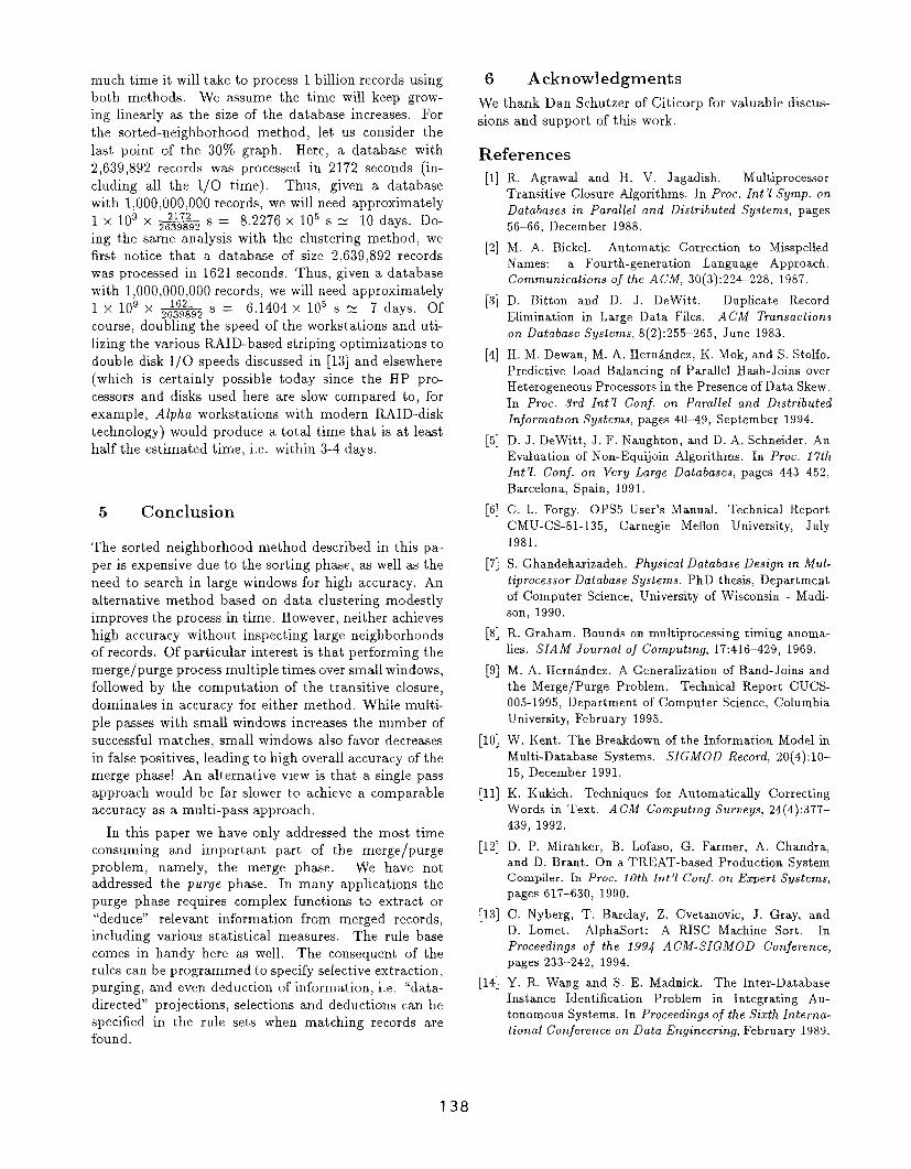
Figure 7: Time performance of the sorted-neighborhood
and clustering methods
Finally, we demonstrate that the sorted neighborhood
and clustering methods scale well as the size of the
database increases. We created 4 databases with no
duplicates of different sizes (.5, 1, 1.5, and 2 x 10⁶
records) and, for each one of them, we selected 107o,
30%, and 50% of its tuples for duplication. We
again ran three concurrent but independent runs of
the sorted-neighborhood method (and the clustering
method), each with a different key, and then computed
the transitive closure of the results. Each independent
run used 4 processors. The results are shown in figure 7.
As expected, the time increases linearly as the size of
the databases increase independent of the duplication
factor.
Using the graphs in figure 7 we can estimate how
4Thus, we generated 12 databases.
137
much time it will take to process 1 billion records using
both methods. We assume the time will keep grow-
ing linearly as the size of the database increases. For
the sorted-neighborhood method, let us consider the
last point of the 30’?lo graph. Here, a database with
2,639,892 records was processed in 2172 seconds (in-
cluding all the 1/0 time). Thus, given a database
with 1,000, 000,000 records, we will need approximately
1X10⁹X -2 s = 8.2276 x 10⁵ s s 10 days. Do-
ing the same analysis with the clustering method, we
first notice that a database of size 2,639,892 records
was processed in 1621 seconds. Thus, given a database
with 1,000,000,000 records, we will need approximately
1X10⁹X -2 s = 6.1404 x 10⁵ s R 7 days. Of
course, doubling the speed of the workstations and uti-
lizing the various RAID-based striping optimizations to
double disk 1/0 speeds discussed in [13] and elsewhere
(which is certainly possible today since the HP pro-
cessors and disks used here are slow compared to, for
example, Alpha workstations with modern RAID-disk
technology) would produce a total time that is at least
half the estimated time, i
5 Conclusion
The sorted neighborhood
e. within 3-4 days.
method described in this pa-
per is expensiv; due to the sorting phase, as well as ~he
need to search in large windows for high accuracy. An
alternative method based on data clustering modestly
improves the process in time. However, neither achieves
high accuracy without inspecting large neighborhoods
of records. Of particular interest is that performing the
merge/purge process multiple times over small windows,
followed by the computation of the transitive closure,
dominates in accuracy for either method. While multi-
ple passes with small windows increases the number of
successful matches, small windows also favor decreases
in false positives, leading to high overall accuracy of the
merge phase! An alternative view is that a single pass
approach would be far slower to achieve a comparable
accuracy as a multi-pass approach.
In this paper we have only addressed the most time
consuming and important part of the merge/purge
problem, namely, the merge phase. We have not
addressed the purge phase. In many applications the
purge phase requires complex functions to extract or
“deduce” relevant information from merged records,
including various statistical measures. The rule base
comes in handy here as well. The consequent of the
rules can be programmed to specify selective extraction,
purging, and even deduction of information, i.e. “data-
directed” projections, selections and deductions can be
specified in the rule sets when matching records are
found.
6 Acknowledgments
We thank Dan Schutzer of Citicorp for valuable discus-
sions and support of this work.
References
[1]
[2]
[3]
[4]
[5]
[6]
[7]
[8]
[9]
[10]
[11]
[12]
[13]
[14]
R. Agrawal and H. V. Jagadish. Multiprocessor
Transitive Closure Algorithms. In Proc. Int’1Syrnp. on
Databases in Parallel and Distributed Systems, pages
56-66, December 1988.
M. A. Bickel. Automatic Correction to Misspelled
Names: a Fourth-generation Language Approach.
Communications of the ACM, 30(3):224-228, 1987.
D. Bitton and D. .J. DeWitt. Duplicate Record
Elimination in Large Data Files. ACM Transactions
on Database Systems, 8(2):255–265, June 1983.
H. M. Dewan, M. A. HernAndez, K. Mok, and S. Stolfo.
Predictive Load Balancing of Parallel Hash-Joins over
Heterogeneous Processors in the Presence of Data Skew.
In Proc. 3rd Int’1 Conf. on Parallel and Distributed
lnformatton Systems, pages 40-49, September 1994.
D. J. DeWitt, J. F. Naughton, and D. A. Schneider. An
Evaluation of Non-Equijoin Algorithms. In Proc. 17th
Int ‘1. C’onf. on Very Large Databases, pages 443-452,
Barcelona, Spain, 1991.
C. L. Forgy. 0PS5 User’s Manual. Technical Report
CMU-CS-81-135, Carnegie Mellon University, July
1981.
S. Ghandeharizadeh. Physical Database Design an Mul-
tiprocessor Database Systems. PhD thesis, Department
of Computer Science, University of Wisconsin - Madi-
son, 1990.
R. Graham. Bounds on multiprocessing timing anoma-
lies. SIAM Journal of Computtngj 17:416-429, 1969.
M. A. Herntindez. A Generalization of Band-Joins and
the Merge/Purge Problem. Technical Report CUCS-
005-1995, Department of Computer Science, Columbia
University, February 1995.
W. Kent. The Breakdown of the Information Model in
Multi-Database Systems. SIGMOD Record, 20(4):10-
15, December 1991.
K. Kukich. Techniques for Automatically Correcting
Words in Text. ACM Computing Surveys, 24(4):377-
439, 1992.
D. P. Miranker, B. Lofaso, G. Farmer, A. Chandra,
and D. Brant. On a TREAT-based Production System
Compiler. In Proc. 10th Int’1 Conf. on Expert Systems,
pages 617-630, 1990.
C. Nyberg, T. Barclay, Z. Cvetanovic, J. Gray, and
D. Lomet. AlphaSort: A RISC Machine Sort. In
Proceedings oj the 1994 A CM- SIGMOD Conference,
pages 233–242, 1994.
Y. R. Wang and S. E. Madnick. The Inter-Database
Instance Identification Problem in Integrating Au-
tonomous Systems. In Proceedings of the Sizth Interna-
tional Conference on Data Engineering, February 1989.
138


