
BIODIVERSITYRESEARCH
The pitfalls of ignoring behaviour whenquantifying habitat selection
C. L. Roever1†*, H. L. Beyer2†, M. J. Chase1,3,4 and R. J. van Aarde1
1Conservation Ecology Research Unit,
Department of Zoology and Entomology,
University of Pretoria, Hatfield 0083, South
Africa, 2ARC Centre of Excellence for
Environmental Decisions, Centre for
Biodiversity & Conservation Science,
University of Queensland, Brisbane, Qld
4072, Australia, 3Elephants Without Borders,
PO Box 682, Kasane, Botswana, 4San Diego
Zoo Institute for Conservation Research, San
Diego Zoo Global, 15600 San Pasqual Valley
Road, Escondido, CA 92027, USA
†These authors contributed equally to this
work.
*Correspondence: Carrie L. Roever.
Conservation Ecology Research Unit,
Department of Zoology and Entomology,
University of Pretoria, Hatfield 0083, South
Africa.
E-mail: [email protected]
ABSTRACT
Aim Habitat selection is a behavioural mechanism by which animals attempt to
maximize their inclusive fitness while balancing competing demands, such as
finding food and rearing offspring while avoiding predation, in a heterogeneous
and changing environment. Different habitat characteristics may be associated
with each of these demands, implying that habitat selection varies depending
on the behavioural motivations of the animal. Here, we investigate behaviour-
specific habitat selection in African elephants and discuss its implications for
distribution modelling and conservation.
Location Northern Botswana, Africa, case study.
Methods We use Bayesian state-space models to characterize location time ser-
ies data of elephants into two behavioural states (encamped and exploratory).
We then develop habitat selection models for each behavioural state and
contrast them to models based on data pooled among behaviours.
Results Spatial predictions of habitat use were often markedly different among
the models. Behaviour-specific and pooled habitat selection models differed in
model structure, the magnitude of model coefficients and the form of the selec-
tion curve (linear or quadratic). Selection was typically strongest in the behav-
iour-specific models, although this varied according to behavioural state and
habitat covariate.
Main conclusions Ignoring behavioural states often had important conse-
quences for quantifying habitat selection. Quantifying selection irrespective of
behaviour (among all behaviours) can obscure important species–habitat rela-
tionships, thereby risking weak or incorrect inferences. Behaviour-specific habi-
tat selection provides greater insight into the process of habitat selection and
can improve predictive habitat selection estimates. As some behaviours are
more relevant to specific conservation objectives than others, focusing on
behaviour-specific selection could improve how habitats are prioritized for
conservation or management.
Keywords
African savanna elephant, behaviour, habitat selection, movement, resource
selection function, state-space model.
INTRODUCTION
Animals must resolve a wide range of competing demands to
survive and reproduce: find food, water and mates, avoid
predators, defend a territory and care for offspring. These
competing demands often mean that animals must prioritize
actions or behaviours to meet one goal at the expense of
another. Good foraging areas, for instance, may also be asso-
ciated with higher mortality risk (Nielsen et al., 2006), or
defending a territory may occur at the cost of acquiring food
(Switalski, 2003). Although some behaviours can occur syn-
chronously as a result of multitasking (Fortin et al., 2004),
many behavioural strategies are employed asynchronously,
often because the habitat characteristics associated with
meeting different needs are spatially segregated. For example,
in an environment where food is patchily distributed, forag-
ing within patches and moving between patches occur
asynchronously (Owen-Smith et al., 2010).
DOI: 10.1111/ddi.12164ª 2013 John Wiley & Sons Ltd http://wileyonlinelibrary.com/journal/ddi 1
Diversity and Distributions, (Diversity Distrib.) (2013) 1–12A
Jou
rnal
of
Cons
erva
tion
Bio
geog
raph
yD
iver
sity
and
Dis
trib
utio
ns

Habitat selection modelling is used to quantify species–
habitat relationships and may contribute to conservation and
management (see Boyce & McDonald, 1999; Chetkiewicz
et al., 2006; Nielsen et al., 2006). However, as a consequence
of competing demands, habitat selection may vary consider-
ably depending on the behavioural priorities of the animal.
Pooling data among behaviours can then result in three
inferential pitfalls when quantifying habitat selection. First, if
behaviours have opposing habitat selection patterns, we may
fail to detect selection. Consequently, a coefficient of zero in
a habitat selection model that averages selection among all
behaviours cannot be used as a basis for suggesting that there
is no selection with respect to that covariate. Second, we
may underestimate the strength of selection and, therefore,
the importance of some habitats to an animal. For example,
strong but infrequent behaviour-specific selection for a criti-
cal habitat may be concealed by weak or no selection for that
habitat at other times. Third, the direction or shape of the
selection curve (how the probability of use changes as a
function of a habitat covariate) is likely to be sensitive to
behaviour. For example, selection for a habitat characteristic
may be positive during one behaviour, yet negative during
another, or a selection curve may be approximately linear for
one behaviour but better represented by a quadratic expres-
sion for another. Incorrect assessment of the importance,
strength and form of selection ultimately reduces the inferen-
tial power of the resulting habitat selection models and has
implications for the utility of these models when applied to
conservation and management. Implicit in the application of
a behaviour-pooled habitat selection model to make predic-
tions of space use in new areas or to different times is the
assumption that the ratio of behaviours from which the
overall selection patterns arise will not change.
Behaviour-specific habitat selection has received limited
attention because habitat selection is often based on location
data (e.g. telemetry data) that lacks a behavioural context
(Beyer et al., 2010). Although the expression of behaviour is
not recorded by satellite collars, behavioural state-space
models (Morales et al., 2004) provide a framework by which
behavioural ‘states’ or ‘modes’ can be estimated based on
path characteristics (Beyer et al., 2013). These methods use
the step length (or movement rate) and turn angle character-
istics of the movement path to classify locations into differ-
ent behavioural states based on a mixture of random walks
(Morales et al., 2004). Here, we use this approach to test for
behavioural differences in habitat selection using elephant
telemetry data as a case study. In the dry season, African
savanna elephants (Loxodonta africana) must fulfil competing
physiological requirements. For instance, individuals must
visit water regularly to meet several physiological needs
(Wright & Luck, 1984; Harris et al., 2008; Loarie et al.,
2009). However, areas near water often are nutritionally
depleted in the dry season (de Beer et al., 2006), so elephants
travel away from water in search of forage. Elephants also
reduce their mortality risk by avoiding human settlements
(Roever et al., 2013a). We use a Bayesian state-space
framework to classify telemetry locations into ‘encamped’
and ‘exploratory’ behavioural states and use resource selec-
tion functions to characterize habitat selection in each state.
We find that the importance, strength and form of selection
differ between behavioural states and among animals. We
conclude that behaviour-specific selection provides greater
insight into species–habitat relationships and offers opportu-
nities for improving predictive estimates of space utilization
that may be relevant for conservation and management.
METHODS
Study area and elephant data
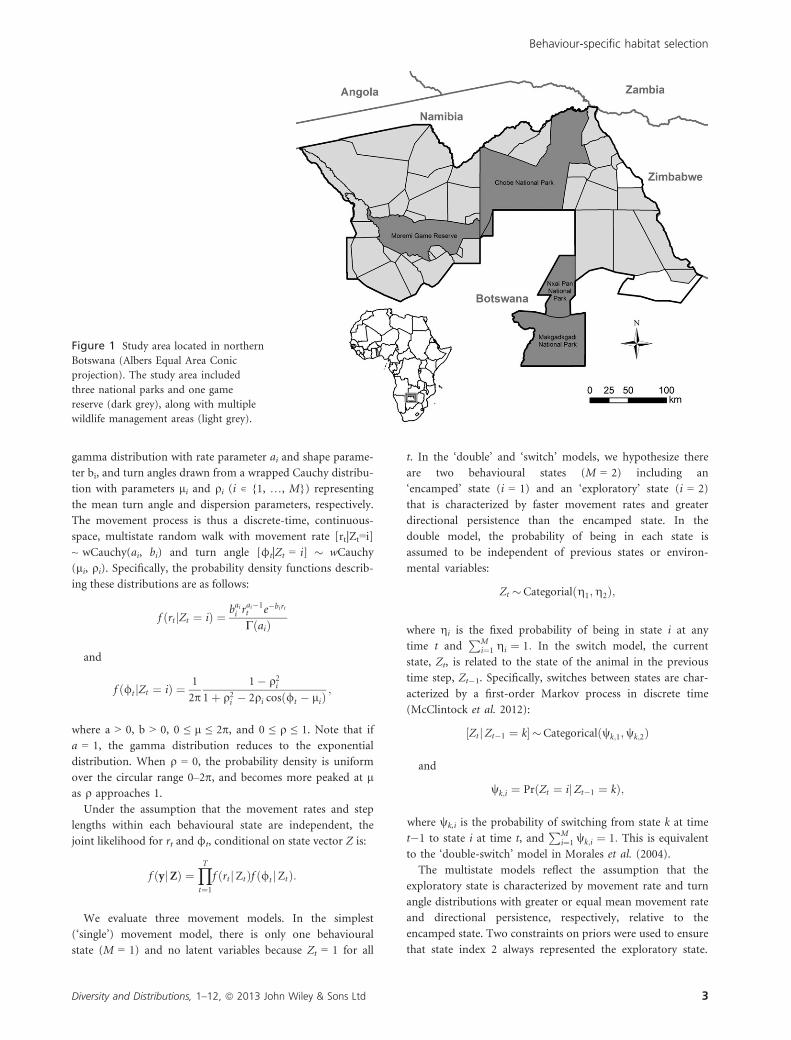
The study area was located in northern Botswana and
included Chobe National Park, Makgadikgadi National Park,
Moremi Game Reserve and Nxai Pan National Park (Fig. 1).
It encompassed an area of 74,355 km2 and was bounded to
the north by Namibia and the east by Zimbabwe. Vegetation
in the study area was primarily deciduous dry woodlands
and interspersed grasslands (Chase, 2011), and terrain in the
region was relatively flat, with the steepest slopes occurring
along the Chobe River. Areas of high human use were mostly
located around the periphery of the study area.
Within the study area, 11 elephants were collared with
GPS collars (Africa Wildlife Tracking, Pretoria, South Africa)
between August 2009 and September 2011. Collars were pro-
gramed to locate animals every hour, and only data from the
2011 dry season (July–November, inclusive) were used in this
analysis. There were more than 1000 locations per individual
for this period, resulting in five females and six males with a
total of 36,023 locations (see Table S1 in Supporting Infor-
mation). For each individual, seasonal ranges were based on
the 95% isopleths of a Gaussian kernel density estimate
(Geospatial Modelling Environment; Beyer, 2011) using
smoothed cross-validation (SCV) bandwidth estimators from
the ‘ks’ library in R (Duong, 2012).
Movement models
Following Morales et al. (2004) and McClintock et al. (2012),
we modelled movement as a combination of one or more dis-
crete-time random walks (RWs), each characterized by distri-
butions of movement rates (rt, the velocity between two
consecutive spatial locations Xt and Xt+1) and turn angles (φt,
the angular difference in direction of travel between two con-
secutive steps, Xt�1 to Xt and Xt to Xt+1). When multiple RWs
are used, each observation yt (t = 1, …, T) must be assigned
to one of the RWs and parameters estimated for the probabil-
ity distributions describing each RW. This can be formulated
as a state-space model, whereby a latent (unobserved) state
indicator Zt = i, i, ∊{1, …, M}, where M is the number of
movement states considered, is used to associate each observa-
tion with a RW (Morales et al., 2004). For each RW, move-
ment rates and turn angles are assumed to be independent and
identically distributed, with movement rates drawn from a
2 Diversity and Distributions, 1–12, ª 2013 John Wiley & Sons Ltd
C. L. Roever et al.
gamma distribution with rate parameter ai and shape parame-
ter bi, and turn angles drawn from a wrapped Cauchy distribu-
tion with parameters li and qi (i ∊ {1, …, M}) representingthe mean turn angle and dispersion parameters, respectively.
The movement process is thus a discrete-time, continuous-
space, multistate random walk with movement rate [rt|Zt=i]~ wCauchy(ai, bi) and turn angle [φt|Zt = i] � wCauchy
(li, qi). Specifically, the probability density functions describ-
ing these distributions are as follows:
f ðrt jZt ¼ iÞ ¼ baii rai�1t e�birt
CðaiÞ
and
f ð/t jZt ¼ iÞ ¼ 1
2p1� q2i
1þ q2i � 2qi cosð/t � liÞ;
where a > 0, b > 0, 0 ≤ l ≤ 2p, and 0 ≤ q ≤ 1. Note that if
a = 1, the gamma distribution reduces to the exponential
distribution. When q = 0, the probability density is uniform
over the circular range 0–2p, and becomes more peaked at las q approaches 1.
Under the assumption that the movement rates and step
lengths within each behavioural state are independent, the
joint likelihood for rt and φt, conditional on state vector Z is:
f ðyjZÞ ¼YT
t¼1
f ðrt jZtÞf ð/t jZtÞ:
We evaluate three movement models. In the simplest
(‘single’) movement model, there is only one behavioural
state (M = 1) and no latent variables because Zt = 1 for all
t. In the ‘double’ and ‘switch’ models, we hypothesize there
are two behavioural states (M = 2) including an
‘encamped’ state (i = 1) and an ‘exploratory’ state (i = 2)
that is characterized by faster movement rates and greater
directional persistence than the encamped state. In the
double model, the probability of being in each state is
assumed to be independent of previous states or environ-
mental variables:
Zt �Categorialðg1;g2Þ;
where ηi is the fixed probability of being in state i at any
time t andPM
i¼1 gi ¼ 1: In the switch model, the current
state, Zt, is related to the state of the animal in the previous
time step, Zt�1. Specifically, switches between states are char-
acterized by a first-order Markov process in discrete time
(McClintock et al. 2012):
½Zt jZt�1 ¼ k� �Categoricalðwk;1;wk;2Þ
and
wk;i ¼ PrðZt ¼ ijZt�1 ¼ kÞ;
where wk,i is the probability of switching from state k at time
t�1 to state i at time t, andPM
i¼1 wk;i ¼ 1: This is equivalent
to the ‘double-switch’ model in Morales et al. (2004).
The multistate models reflect the assumption that the
exploratory state is characterized by movement rate and turn
angle distributions with greater or equal mean movement rate
and directional persistence, respectively, relative to the
encamped state. Two constraints on priors were used to ensure
that state index 2 always represented the exploratory state.
Figure 1 Study area located in northern
Botswana (Albers Equal Area Conic
projection). The study area included
three national parks and one game
reserve (dark grey), along with multiple
wildlife management areas (light grey).
Diversity and Distributions, 1–12, ª 2013 John Wiley & Sons Ltd 3
Behaviour-specific habitat selection
Without these constraints, the two states can be assigned dif-
ferent index values (1 or 2) among MCMC chains, and these
values can even switch within a single MCMC chain, compli-
cating the interpretation of the posterior samples. The means
of the encamped (�r1) and exploratory (�r2) gamma distribu-
tions were sampled using priors �r1 �Uð0; 1:6Þ and
�r2 �Uð0; 1:6Þ þ �r1, where U(0, 1.6) is a uniform distribution
in the range 0–1.6 (1.6 was the maximum movement rate
observed among all steps and animals). The two rate parame-
ters of the gamma distributions (a1, a2) were then sampled
from vague priors (a1~ gamma(0.001, 0.001), a2~gamma
(0.001, 0.001), and the shape parameters (b1, b2) were calcu-
lated deterministically by dividing the rate parameter by the
mean (b1 ¼ a1=�r1; b2 ¼ a2=�r2). The priors for the dispersion
parameters of the wrapped Cauchy distribution, q1 and q2,involved sampling two random variables from uniform distri-
butions in the range [0, 1] and assigning the smaller of them
to q1. All other variables were sampled from vague priors. Spe-
cifically, g and w were sampled from uniform distributions in
the range [0, 1], and l was sampled from a uniform distribu-
tion over the range [0–10p] (the large range here helps to
prevent boundary effects in the posteriors for l).Models were fitted using Monte Carlo Markov Chain
(MCMC) techniques implemented in the software JAGS
(Plummer, 2003) using three chains with a burn-in period of
10,000 samples, which were discarded, followed by 50,000
samples, thinned to retain every 25th sample, resulting in
2000 independent samples per chain from the posterior dis-
tribution of each parameter. Chains were initialized by sam-
pling from the prior distributions (see Appendix S1 for full
details). Every model was checked for convergence to a sta-
tionary distribution using the Gelman–Rubin convergence
statistic (R; Gelman & Rubin, 1992), whereby R < 1.1 indi-
cated convergence, and by visually examining plots of the
chains and autocorrelation plots for each chain. R was calcu-
lated using the ‘gelman.diag’ function in the ‘coda’ library in
R (R Development Core Team, 2011). Model selection was
informed by the widely applicable information criteria
(WAIC; Watanabe, 2010).
Resource selection models
Using the top-ranked movement model for each individual,
we partitioned the telemetry locations into encamped and
exploratory behavioural states and quantified habitat selec-
tion for each behavioural state and for the pooled data (all
telemetry locations irrespective of behavioural state).
Resource selection for each individual was estimated by com-
paring the telemetry locations to random locations using the
logistic form of the resource selection probability function
(Manly et al., 2002; Lele & Keim, 2006). Random locations
were generated within the seasonal range of each individual
at a density of 12 points per km2. The same set of random
locations was used for the pooled, encamped and exploratory
habitat selection models.
Selection was quantified for habitat covariates known to
influence elephant habitat selection (Roever et al., 2012). Ele-
phants are known to respond to water, slope, vegetative
cover and human presence. The spatial location of water was
mapped using community contributed GPS data from
Tracks4Africa (Pretoria, South Africa) and was manually val-
idated using Landsat imagery. In northern Botswana, water
other than in rivers is scarce during the dry season; therefore,
we used only water bodies classified as main rivers, river del-
tas, dams and man-made watering holes for this dry season
analysis. Distance to water was calculated for all landscape
locations. Slope was calculated from a 90 m digital elevation
model (Jarvis et al., 2006), and percentage tree cover at a
500 m resolution was obtained from Moderate Resolution
Imaging Spectrometer (MODIS) Vegetation Continuous
Fields product (Hansen et al., 2006). The 500 m tree cover
layer was resampled to a 90 m resolution using a cubic con-
volution interpolation to match the resolution of the other
datasets. Finally, human density data at a 1 km resolution
were obtained from LandScan (2008) daily human popula-
tion data. Hoare & du Toit (1999) found that elephants
avoid areas with greater than 16 people km�2, so we identi-
fied all areas with human densities greater than this value
and calculated distance to these high human-use areas. All
geospatial analysis was completed using the Spatial Analyst
extension of ArcGIS 10.0 (ESRI, Redlands, CA, USA) and
Geospatial Modelling Environment (Beyer, 2011).
Using the suite of habitat covariates described, five candi-
date models were formulated (Table 1), and Bayesian infor-
mation criterion (BIC; Schwarz, 1978) was used to identify
the top-ranked habitat selection model for the two behavio-
ural state datasets and the pooled dataset of each individual.
Covariates with Pearson’s r > 0.6 were not included in the
same model. For six individuals, distance to water was corre-
lated with distance to humans, so only candidate models 1
Table 1 Competing habitat selection models relating habitat use to distance to water (‘water’), percentage tree cover (‘tree’), slope and
distance to human settlement (‘human’). The number of parameters (K) includes an intercept term. Models were fit to behavioural
state-specific and pooled datasets and ranked using BIC
Name Candidate model K
1. Landscape Water + tree + slope 4
2. Landscape (nonlinear) Water + (water)2 + tree + (tree)2 + slope 6
3. No Slope Water + (water)2 + tree + (tree)2 + human + (human)2 7
4. Full (humans linear) Water + (water)2 + tree + (tree)2 + slope + human 7
5. Full Water + (water)2 + tree + (tree)2 + slope + human + (human)2 8
4 Diversity and Distributions, 1–12, ª 2013 John Wiley & Sons Ltd
C. L. Roever et al.
and 2 were evaluated. To assess the fit of the top-ranked
model for each individual, we used k-fold cross-validation
(k = 5), whereby, for each individual, a model is iteratively
(k times) fit to 80% (1�N/k) of the data and validated using
the remaining 20% (N/k) of the data. Fit is quantified using
the Spearman rank correlation coefficient based on the fre-
quency of used points in each of 10 equal area bins of pre-
dicted values (see Boyce et al., 2002). For the pooled model,
the full dataset was used for fitting and validation, while only
the data corresponding to each behavioural state were used
to fit and validate the behaviour-specific models. Selection
probabilities for habitat covariates were calculated using:
wðxÞ ¼ eXb=ð1þ eXbÞ;
where w(x) is the resource selection probability function, X
is a matrix of habitat covariates (including a column of one’s
representing the intercept term) and b is the vector of maxi-
mum likelihood estimates of the model coefficients. To assess
overall predictive power, we compared the model fit of the
pooled model against a behaviourally averaged model,
bðxÞ ¼ PMi¼1 piwðxiÞ, for each individual where pi is the pro-
portion of locations in the ith behavioural state and w(xi) is
the resource selection model for that state. We quantified
model fit of both the pooled and averaged model using the
Spearman rank correlation coefficient as described above.
Finally, to test whether selection for habitat covariates dif-
fered significantly between the encamped and exploratory
states, we contrasted exploratory (0) and encamped (1) data
for each individual using latent selection difference (LSD)
functions (Czetwertynski, 2007; Latham et al., 2011). Because
availability remains constant across behavioural states for
each individual, this model provides direct comparisons of
selection with significance and strength measures (Czetwer-
tynski, 2007). For each individual, the same model structure
was used as in the top-ranked model from the use versus
available analysis; however, if model structure between the
encamped and exploratory state differed, we used the more
complete model. To reduce the probability of a Type I error
resulting from serially correlated telemetry data, we used
Newey–West variance inflation when estimating standard
errors (Newey & West, 1987; Nielsen et al., 2002). Using
autocorrelation functions (ACF), we found evidence of tem-
poral autocorrelation in the step lengths of individuals every
12 hours in the pooled elephant data. This pattern was cor-
roborated with the classified behavioural data, as the mean
time an individual spent in the same state ranged from 3 to
12 hours among individual. To be conservative, we used a
lag of 12 for all individuals and models. All analysis was
conducted in R (R Development Core Team, 2011) using the
‘ResourceSelection’ library (Lele et al., 2011).
RESULTS
The switch model, in which the probability of switching
between states was explicitly estimated, was the top-ranked
movement model for most (9 of 11) individuals (see Table
S2-3). However, for males EM0190 and EM0198 the double
model, which indicated that switching probabilities among
states could be reasonably approximated as constants, was the
top-ranked model. Although the switch model was the highest-
ranked model using WAIC for animal EM0195, it was charac-
terized by long periods (> 18 days) of no state switching. This
was not consistent with our knowledge of elephant behaviour
and was not supported by the double model, so for this animal,
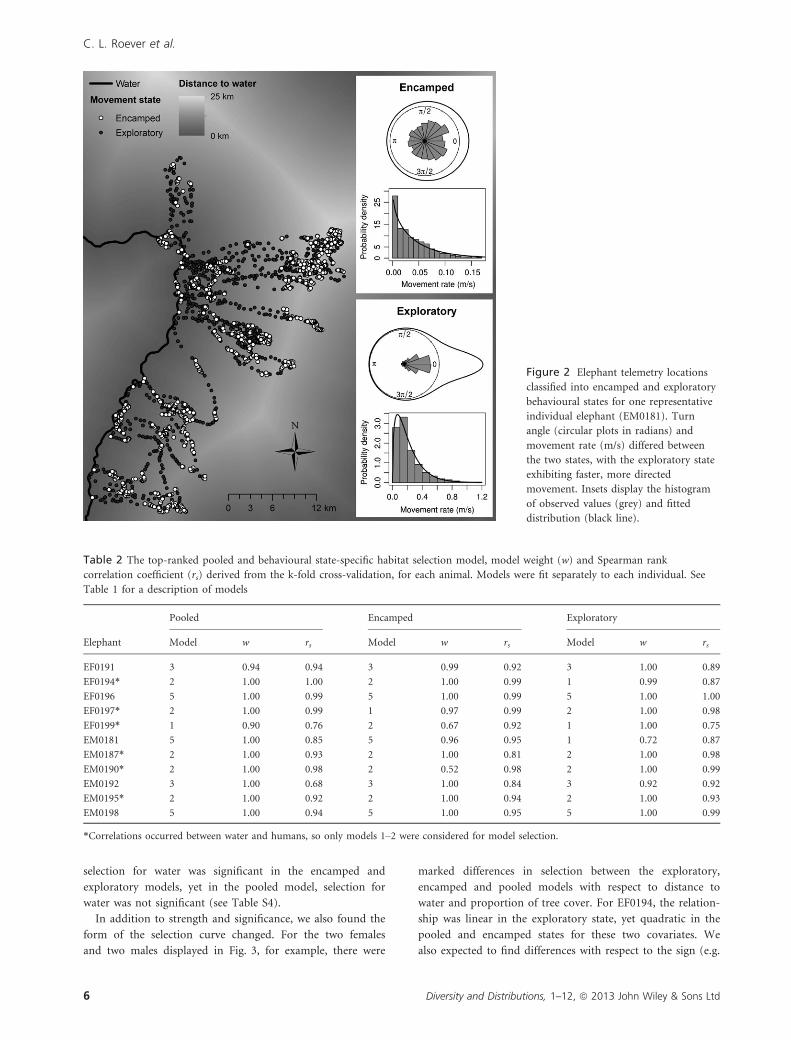
we used the double model. In all cases, the behavioural state
models far out-ranked the reference model (the single behavio-
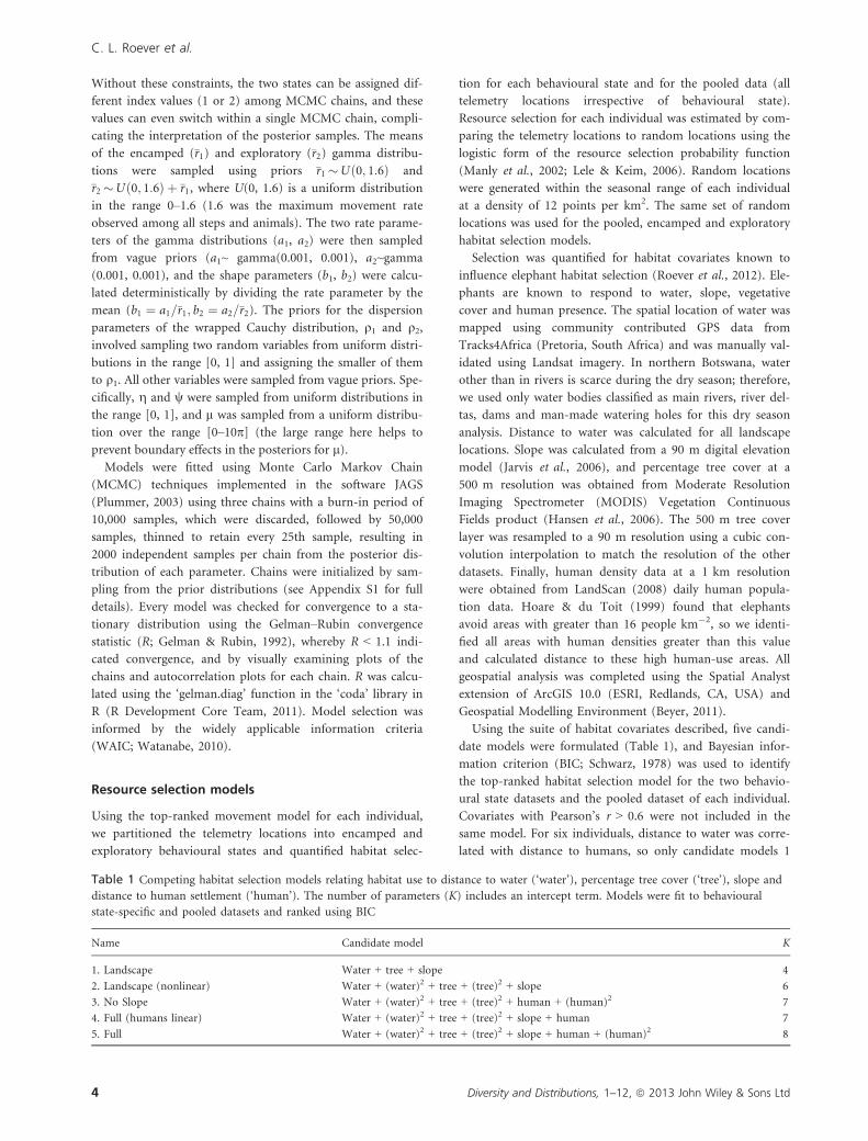
ural state model). Locations classified as exploratory had
longer step lengths and greater directional persistence than
points classified as encamped, which were generally clumped
with shorter step lengths and larger turn angles (Fig. 2).
The model structure of the pooled and behaviour-specific
habitat selection models sometimes differed. While 7 of 11
individuals had top-ranked model structure that did not
vary among behavioural states (pooled, encamped, explor-
atory), for four elephants, the encamped or exploratory
model structure differed from that of the other two models
(Table 2). When model structure varied between behaviour-
al states, the pooled model structure did not consistently
resemble one movement state preferentially. Instead, the
pooled model structure was generally the same as the
behavioural state with the most complex structure (i.e. with
the most covariates).
The top-ranked habitat selection models provided good
fit to the data using k-fold cross-validation tested with the
Spearman rank correlation coefficient (rs ≥ 0.68, P < 0.05)
for all elephants (Table 2). For EM0192, the pooled model
fit was relatively low (rs = 0.68, P < 0.05), but the
encamped (rs = 0.84, P < 0.01) and exploratory (rs = 0.92,
P < 0.01) model fit was better. Averaging the behaviour-
specific models for EM0192 into a behaviourally averaged
model then provided moderately better fit (rs = 0.96,
P < 0.01) than the pooled model, which did not incorpo-
rate behaviour; however, fit of both models was signifi-
cantly positive. For all other elephants, the behaviour-
averaged model and the pooled model performed equally
well (see Fig. S1).
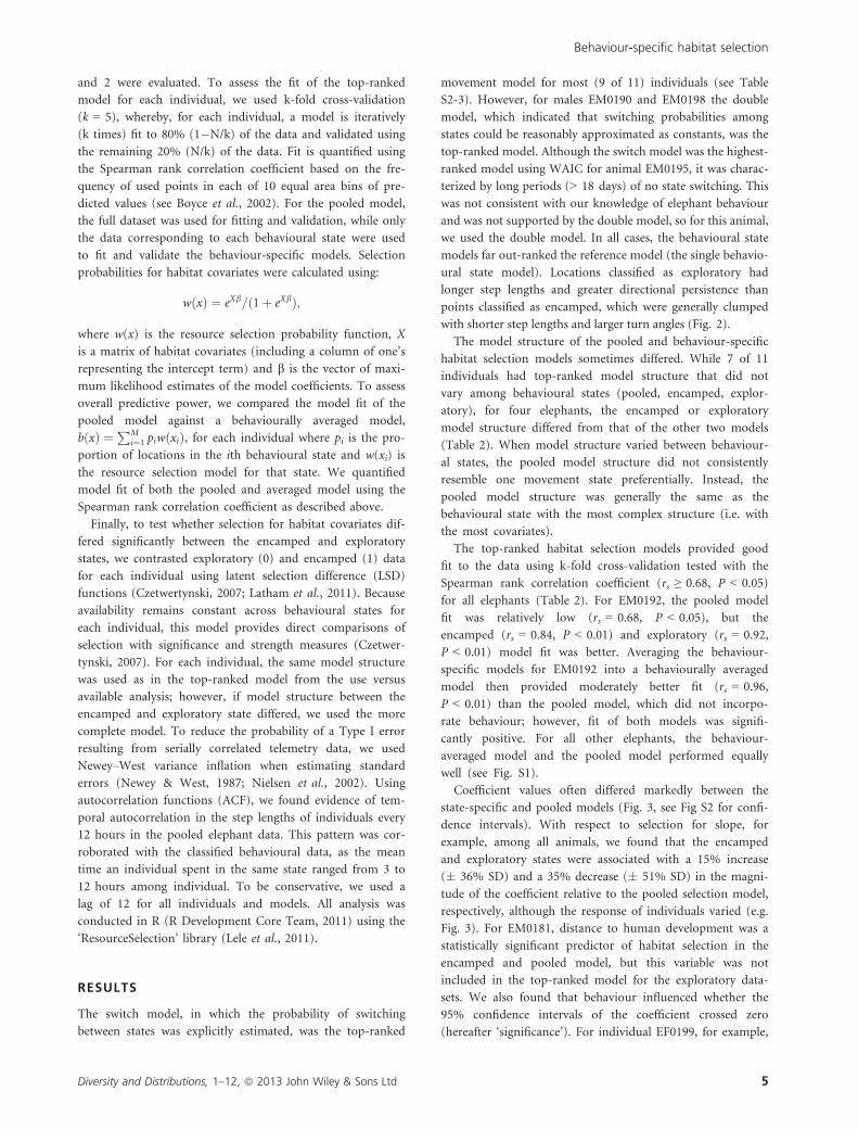
Coefficient values often differed markedly between the
state-specific and pooled models (Fig. 3, see Fig S2 for confi-
dence intervals). With respect to selection for slope, for
example, among all animals, we found that the encamped
and exploratory states were associated with a 15% increase
(� 36% SD) and a 35% decrease (� 51% SD) in the magni-
tude of the coefficient relative to the pooled selection model,
respectively, although the response of individuals varied (e.g.
Fig. 3). For EM0181, distance to human development was a
statistically significant predictor of habitat selection in the
encamped and pooled model, but this variable was not
included in the top-ranked model for the exploratory data-
sets. We also found that behaviour influenced whether the
95% confidence intervals of the coefficient crossed zero
(hereafter ‘significance’). For individual EF0199, for example,
Diversity and Distributions, 1–12, ª 2013 John Wiley & Sons Ltd 5
Behaviour-specific habitat selection
selection for water was significant in the encamped and
exploratory models, yet in the pooled model, selection for
water was not significant (see Table S4).
In addition to strength and significance, we also found the
form of the selection curve changed. For the two females
and two males displayed in Fig. 3, for example, there were
marked differences in selection between the exploratory,
encamped and pooled models with respect to distance to
water and proportion of tree cover. For EF0194, the relation-
ship was linear in the exploratory state, yet quadratic in the
pooled and encamped states for these two covariates. We
also expected to find differences with respect to the sign (e.g.
Figure 2 Elephant telemetry locations
classified into encamped and exploratory
behavioural states for one representative
individual elephant (EM0181). Turn
angle (circular plots in radians) and
movement rate (m/s) differed between
the two states, with the exploratory state
exhibiting faster, more directed
movement. Insets display the histogram
of observed values (grey) and fitted
distribution (black line).
Table 2 The top-ranked pooled and behavioural state-specific habitat selection model, model weight (w) and Spearman rank
correlation coefficient (rs) derived from the k-fold cross-validation, for each animal. Models were fit separately to each individual. See
Table 1 for a description of models
Elephant
Pooled Encamped Exploratory
Model w rs Model w rs Model w rs
EF0191 3 0.94 0.94 3 0.99 0.92 3 1.00 0.89
EF0194* 2 1.00 1.00 2 1.00 0.99 1 0.99 0.87
EF0196 5 1.00 0.99 5 1.00 0.99 5 1.00 1.00
EF0197* 2 1.00 0.99 1 0.97 0.99 2 1.00 0.98
EF0199* 1 0.90 0.76 2 0.67 0.92 1 1.00 0.75
EM0181 5 1.00 0.85 5 0.96 0.95 1 0.72 0.87
EM0187* 2 1.00 0.93 2 1.00 0.81 2 1.00 0.98
EM0190* 2 1.00 0.98 2 0.52 0.98 2 1.00 0.99
EM0192 3 1.00 0.68 3 1.00 0.84 3 0.92 0.92
EM0195* 2 1.00 0.92 2 1.00 0.94 2 1.00 0.93
EM0198 5 1.00 0.94 5 1.00 0.95 5 1.00 0.99
*Correlations occurred between water and humans, so only models 1–2 were considered for model selection.
6 Diversity and Distributions, 1–12, ª 2013 John Wiley & Sons Ltd
C. L. Roever et al.

positive or negative) of the selection coefficient; however, for
the elephants examined here, we found very few sign
changes. All of the differences we did observe were associated
with quadratic covariates, resulting in changes to the form of
the quadratic function. While selection for steeper slopes was
consistent across the four animals in the example, the
strength (i.e. slope) of the selection coefficients varied.
The differences in habitat selection coefficients identified
between the encamped and exploratory states were significant
in many cases (Table 3). For most individuals (9 of 11), we
found significant differences in selection for at least one hab-
itat covariate between the encamped and exploratory
behavioural states. For six of these individuals, selection var-
ied significantly for two or more habitat covariates. These
0
0.8
0 10 20 30
EF01
94Se
lect
ion
Prob
abili
ty
0
0.7
0.00 0.11 0.22 0.330.0
1.0
0 2 4 6
0
0.7
0 7 14 21
EF01
97Se
lect
ion
Prob
abili
ty
0
0.6
0.00 0.15 0.30 0.450.0
1.0
0 1 2 3
0.0
0.3
0 7 14 21
EM01
81Se
lect
ion
Prob
abili
ty
0
0.12
0.00 0.07 0.14 0.210.0
0.4
0 2 3 5
0.0
1.0
0 20 40
EM01
90Se
lect
ion
Prob
abili
ty
Distance to water (km)
0
0.4
0.00 0.10 0.20
Proportion tree cover
0.0
1.0
0 1 2 3
Slope (degrees)
Figure 3 Probability of selection for distance to water, proportion of tree cover and slope as a function of behavioural state for four
representative elephants. Selection in the pooled model (solid line) differed in importance, strength and form of selection (e.g. linear
versus quadratic) from the encamped (short dashed line) and exploratory (long dashed line) behavioural state models.
Diversity and Distributions, 1–12, ª 2013 John Wiley & Sons Ltd 7
Behaviour-specific habitat selection
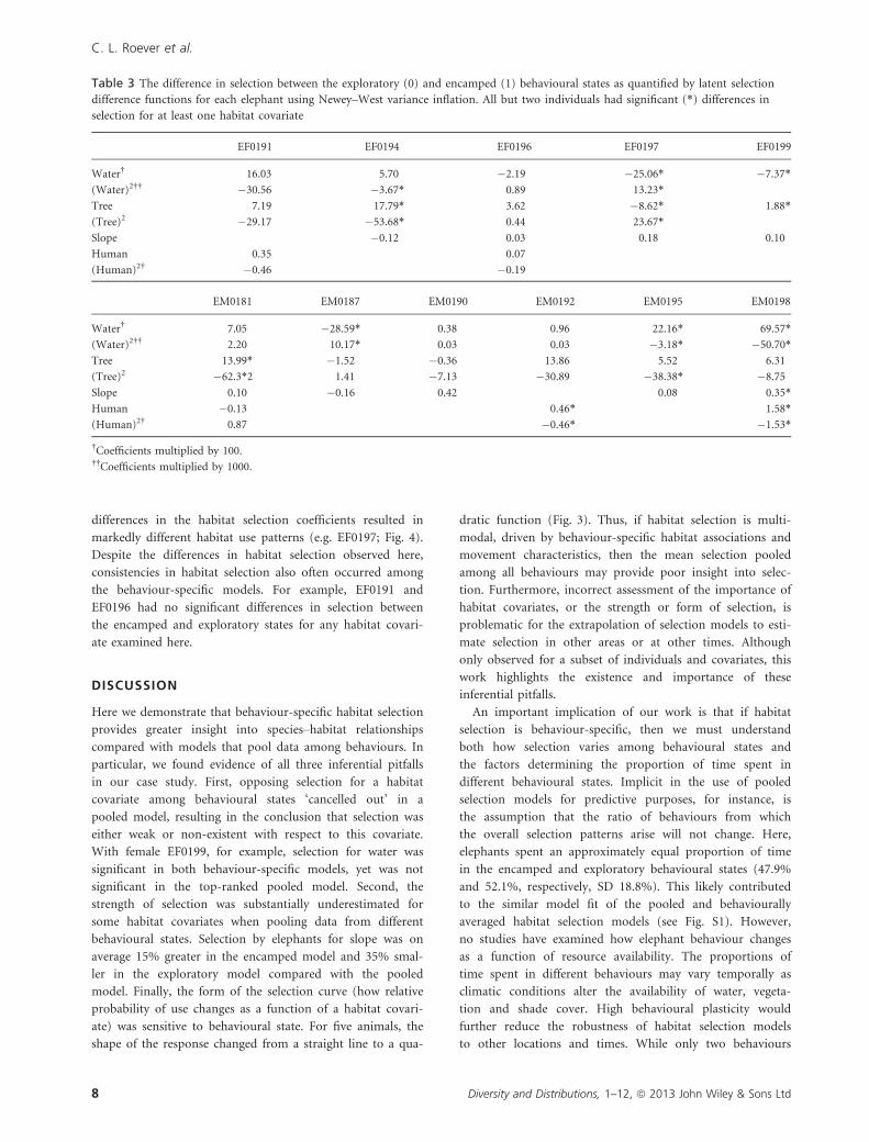
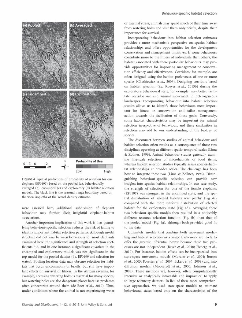
differences in the habitat selection coefficients resulted in
markedly different habitat use patterns (e.g. EF0197; Fig. 4).
Despite the differences in habitat selection observed here,
consistencies in habitat selection also often occurred among
the behaviour-specific models. For example, EF0191 and
EF0196 had no significant differences in selection between
the encamped and exploratory states for any habitat covari-
ate examined here.
DISCUSSION
Here we demonstrate that behaviour-specific habitat selection
provides greater insight into species–habitat relationships
compared with models that pool data among behaviours. In
particular, we found evidence of all three inferential pitfalls
in our case study. First, opposing selection for a habitat
covariate among behavioural states ‘cancelled out’ in a
pooled model, resulting in the conclusion that selection was
either weak or non-existent with respect to this covariate.
With female EF0199, for example, selection for water was
significant in both behaviour-specific models, yet was not
significant in the top-ranked pooled model. Second, the
strength of selection was substantially underestimated for
some habitat covariates when pooling data from different
behavioural states. Selection by elephants for slope was on
average 15% greater in the encamped model and 35% smal-
ler in the exploratory model compared with the pooled
model. Finally, the form of the selection curve (how relative
probability of use changes as a function of a habitat covari-
ate) was sensitive to behavioural state. For five animals, the
shape of the response changed from a straight line to a qua-
dratic function (Fig. 3). Thus, if habitat selection is multi-
modal, driven by behaviour-specific habitat associations and
movement characteristics, then the mean selection pooled
among all behaviours may provide poor insight into selec-
tion. Furthermore, incorrect assessment of the importance of
habitat covariates, or the strength or form of selection, is
problematic for the extrapolation of selection models to esti-
mate selection in other areas or at other times. Although
only observed for a subset of individuals and covariates, this
work highlights the existence and importance of these
inferential pitfalls.
An important implication of our work is that if habitat
selection is behaviour-specific, then we must understand
both how selection varies among behavioural states and
the factors determining the proportion of time spent in
different behavioural states. Implicit in the use of pooled
selection models for predictive purposes, for instance, is
the assumption that the ratio of behaviours from which
the overall selection patterns arise will not change. Here,
elephants spent an approximately equal proportion of time
in the encamped and exploratory behavioural states (47.9%
and 52.1%, respectively, SD 18.8%). This likely contributed
to the similar model fit of the pooled and behaviourally
averaged habitat selection models (see Fig. S1). However,
no studies have examined how elephant behaviour changes
as a function of resource availability. The proportions of
time spent in different behaviours may vary temporally as
climatic conditions alter the availability of water, vegeta-
tion and shade cover. High behavioural plasticity would
further reduce the robustness of habitat selection models
to other locations and times. While only two behaviours
Table 3 The difference in selection between the exploratory (0) and encamped (1) behavioural states as quantified by latent selection
difference functions for each elephant using Newey–West variance inflation. All but two individuals had significant (*) differences inselection for at least one habitat covariate
EF0191 EF0194 EF0196 EF0197 EF0199
Water† 16.03 5.70 �2.19 �25.06* �7.37*
(Water)2†† �30.56 �3.67* 0.89 13.23*
Tree 7.19 17.79* 3.62 �8.62* 1.88*
(Tree)2 �29.17 �53.68* 0.44 23.67*
Slope �0.12 0.03 0.18 0.10
Human 0.35 0.07
(Human)2† �0.46 �0.19
EM0181 EM0187 EM0190 EM0192 EM0195 EM0198
Water† 7.05 �28.59* 0.38 0.96 22.16* 69.57*
(Water)2†† 2.20 10.17* 0.03 0.03 �3.18* �50.70*
Tree 13.99* �1.52 �0.36 13.86 5.52 6.31
(Tree)2 �62.3*2 1.41 �7.13 �30.89 �38.38* �8.75
Slope 0.10 �0.16 0.42 0.08 0.35*
Human �0.13 0.46* 1.58*
(Human)2† 0.87 �0.46* �1.53*
†Coefficients multiplied by 100.††Coefficients multiplied by 1000.
8 Diversity and Distributions, 1–12, ª 2013 John Wiley & Sons Ltd
C. L. Roever et al.
were assessed here, additional subdivision of elephant
behaviour may further elicit insightful elephant-habitat
associations.
Another important implication of this work is that quanti-
fying behaviour-specific selection reduces the risk of failing to
identify important habitat selection patterns. Although model
structure did not vary between behaviours for most elephants
examined here, the significance and strength of selection coef-
ficients did, and in one instance, a significant covariate in the
encamped and exploratory models was not significant in the
top model for the pooled dataset (i.e. EF0199 and selection for
water). Pooling location data may obscure selection for habi-
tats that occur uncommonly or briefly, but still have impor-
tant effects on survival or fitness. In the African savanna, for
example, accessing watering holes is essential for many species,
but watering holes are also dangerous places because predators
often concentrate around them (de Boer et al., 2010). Thus,
under conditions where the animal is not experiencing water
or thermal stress, animals may spend much of their time away
from watering holes and visit them only briefly, despite their
importance for survival.
Incorporating behaviour into habitat selection estimates
provides a more mechanistic perspective on species–habitat
relationships and offers opportunities for the development
conservation and management initiatives. If some behaviours
contribute more to the fitness of individuals than others, the
habitat associated with these particular behaviours may pro-
vide opportunities for improving management or conserva-
tion efficiency and effectiveness. Corridors, for example, are
often designed using the habitat preferences of one or more
species (Chetkiewicz et al., 2006). Designing corridors based
on habitat selection (i.e. Roever et al., 2013b) during the
exploratory behavioural state, for example, may better facili-
tate corridor use and animal movement in heterogeneous
landscapes. Incorporating behaviour into habitat selection
studies allows us to identify those behaviours most impor-
tant for fitness or conservation and tailor management
action towards the facilitation of those goals. Conversely,
some habitat characteristics may be important for animal
selection irrespective of behaviour, and these similarities in
selection also add to our understanding of the biology of
species.
The disconnect between studies of animal behaviour and
habitat selection often results as a consequence of those two
disciplines operating at different spatio-temporal scales (Lima
& Zollner, 1996). Animal behaviour studies generally exam-
ine fine-scale selection of microhabitats or food items,
whereas habitat selection studies typically assess species–habi-
tat relationships at broader scales. The challenge has been
how to integrate these two (Lima & Zollner, 1996). Distin-
guishing behaviour-specific selection can provide new
insights into species–habitat relationships. In our case study,
the strength of selection for one of the female elephants
(EF0197) was strongest in the encamped state, and the spa-
tial distribution of selected habitats was patchy (Fig. 4c)
compared with the more uniform distribution of selected
habitat for the exploratory state (Fig. 4d). Averaging these
two behaviour-specific models then resulted in a noticeably
different resource selection function (Fig. 4b) than that of
the pooled model (Fig. 4a), although both provided good fit
to the data.
Ultimately, models that combine both movement model-
ling and habitat selection in a single framework are likely to
offer the greatest inferential power because these two pro-
cesses are not independent (Beyer et al., 2010; Fieberg et al.,
2010). For instance, habitat effects can be incorporated into
state-space movement models (Morales et al., 2004; Jonsen
et al., 2005; Forester et al., 2007; Eckert et al., 2008) and into
diffusion models (Moorcroft et al., 2006; Johnson et al.,
2008). These methods are, however, often computationally
intensive or analytically intractable and impractical to apply
to large telemetry datasets. In lieu of these more comprehen-
sive approaches, we used state-space models to estimate
behavioural states based only on the characteristics of the
(a) (b)
(c) (d)
Figure 4 Spatial predictions of probability of selection for one
elephant (EF0197) based on the pooled (a), behaviourally
averaged (b), encamped (c) and exploratory (d) habitat selection
models. The black line is the seasonal range boundary based on
the 95% isopleths of the kernel density estimate.
Diversity and Distributions, 1–12, ª 2013 John Wiley & Sons Ltd 9
Behaviour-specific habitat selection

movement paths (but not habitat covariates), and we subse-
quently quantified habitat selection using generalized linear
models for each animal. Although not an ideal solution, it
does demonstrate the premise of this work that resource
selection is behaviour specific.
Using more mechanistic models of species–habitat rela-
tionships at the level of the individual may also improve our
ability to predict distribution at the population level,
although scaling up from individuals to populations is not
straightforward. Selection varies as a function of the samples
of use and availability, making it difficult to directly compare
selection quantified over different availabilities (Beyer et al.,
2010). Although one common approach to making popula-
tion-level inferences is to estimate population-averaged selec-
tion (e.g. the marginal inferences from a generalized linear
mixed model where individual is treated as a random effect),
it might be better to quantify selection in terms of functional
responses (Mysterud & Ims, 1998), whereby selection is
modelled as a function of the availabilities of all habitats
(Mathiopoulos et al., 2011). By explicitly quantifying how
selection changes as availability changes, predictions from
functional response models are likely to be more robust
when applied to new regions (where animals were not sam-
pled). Using a functional response model to make spatial
predictions of population distribution requires an under-
standing of how social interactions affect availability (i.e.
determining an appropriate scale over which to assess avail-
ability to apply the functional response model), which is an
area of active research.
In conservation, the aim of habitat selection studies is
often to predict changes in habitat use based on some future
scenario, alternative management strategy, or predict species
distribution in a new region. Yet if we fail to understand the
processes driving selection, our projections and any subse-
quent inferences could be weak or incorrect. By incorporat-
ing behavioural processes into habitat selection, we might
move a step beyond describing patterns to better under-
standing the behavioural mechanisms that drive selection
processes (Beyer et al., 2010). As habitat selection studies are
applied increasingly to conservation issues such as reserve
and corridor design (e.g. Cabeza et al., 2004; Chetkiewicz &
Boyce, 2009; Roever et al., 2013b), it is imperative that esti-
mates are robust and that habitat is appropriately character-
ized in ways that are most relevant to the survival and,
ultimately, fitness of wildlife species.
ACKNOWLEDGEMENTS
We would like to thank the International Fund for Animal
Welfare (IFAW), the University of Pretoria, the Australian
Research Council (ARC) Centre of Excellence for Environ-
mental Decisions (CEED) and the Environmental Decisions
Group at the University of Queensland for research fund-
ing and support. GIS data were provided by Tracks4Africa,
and the research was sanctioned and supported by the
Botswana Department of Wildlife & National Parks. Ele-
phants Without Borders was funded by the Paul G. Allen
Family Foundation, Jody Allen, Zoological Society of San
Diego, Madeleine and Jerry Delman Cohen, Harry Fergu-
son, Botswana Government Conservation Trust Fund and
Wilderness Trust. We acknowledge the in kind logistical
support of Cyril Taolo, Larry Patterson, Peter Perlstein,
Mike Holding and Abu Camp. We thank Hugh Possing-
ham for his comments, and we are grateful to Juan M.
Morales for his insightful comments on our Bayesian
analysis.
REFERENCES
de Beer, Y., Kilian, W., Versfeld, W. & van Aarde, R.J.
(2006) Elephants and low rainfall alter woody vegetation in
Etosha National Park, Namibia. Journal of Arid Environ-
ments, 64, 412–421.
Beyer, H.L. (2011) Geospatial Modelling Environment. Spatial
Ecology, LLC. Available at: http://www.spatialecology.com/
gme/ (accessed April 2012).
Beyer, H.L., Haydon, D.T., Morales, J.M., Frair, J.L., Hebble-
white, M., Mitchell, M. & Matthiopoulos, J. (2010) The
interpretation of habitat preference metrics under use-
availability designs. Philosophical Transactions of the Royal
Society B-Biological Sciences, 365, 2245–2254.
Beyer, H.L., Morales, J.M., Murray, D.L. & Fortin, M.-J.
(2013) Estimating behavioural states from movement paths
using Bayesian state-space models: a proof of concept.
Methods in Ecology and Evolution, 4, 433–441.
de Boer, W.F., Vis, M.J.P., de Knegt, H.J., Rowles, C., Kohi,
E.M., van Langevelde, F., Peel, M., Pretorius, Y., Skidmore,
A.K., Slotow, R., van Wieren, S.E. & Prins, H.H.T. (2010)
Spatial distribution of lion kills determined by the water
dependency of prey species. Journal of Mammalogy, 91,
1280–1286.
Boyce, M.S. & McDonald, L.L. (1999) Relating populations
to habitats using resource selection functions. Trends in
Ecology & Evolution, 14, 268–272.
Boyce, M.S., Vernier, P.R., Nielsen, S.E. & Schmiegelow,
F.K.A. (2002) Evaluating resource selection functions. Eco-
logical Modelling, 157, 281–300.
Cabeza, M., Araujo, M.B., Wilson, R.J., Thomas, C.D.,
Cowley, M.J.R. & Moilanen, A. (2004) Combining proba-
bilities of occurrence with spatial reserve design. Journal of
Applied Ecology, 41, 252–262.
Chase, M. (2011) Dry season fixed-wing aerial survey of
elephants and wildlife in northern Botswana, September - Nov-
ermber 2010. Tech. Rep, Elephants Without Borders, Kasane.
Chetkiewicz, C.L.B. & Boyce, M.S. (2009) Use of resource
selection functions to identify conservation corridors. Jour-
nal of Applied Ecology, 46, 1036–1047.
Chetkiewicz, C.-L.B., Clair, C.C.S. & Boyce, M.S. (2006) Cor-
ridors for conservation: integrating pattern and process.
Annual Review of Ecology Evolution and Systematics, 37,
317–342.
10 Diversity and Distributions, 1–12, ª 2013 John Wiley & Sons Ltd
C. L. Roever et al.
Czetwertynski, S.M. (2007) Effects of hunting on the demo-
graphics, movement, and habitat selection of American black
bears (Ursus americanus). University of Alberta, Edmonton.
Duong, T. (2012) ks: Kernel smoothing. R package version
1.8.7. Available at: http://CRAN.R-project.org/package=ks
(accessed April 2012).
Eckert, S.A., Moore, J.E., Dunn, D.C., van Buiten, R.S.,
Eckert, K.L. & Halpin, P.N. (2008) Modeling loggerhead
turtle movement in the Mediterranean: importance of
body size and oceanography. Ecological Applications, 18,
290–308.
Fieberg, J., Matthiopoulos, J., Hebblewhite, M., Boyce, M.S.
& Frair, J.L. (2010) Correlation and studies of habitat
selection: problem, red herring or opportunity? Philosophi-
cal Transactions of the Royal Society B-Biological Sciences,
365, 2233–2244.
Forester, J.D., Ives, A.R., Turner, M.G., Anderson, D.P., For-
tin, D., Beyer, H.L., Smith, D.W. & Boyce, M.S. (2007)
State-space models link elk movement patterns to land-
scape characteristics in Yellowstone National Park. Ecologi-
cal Monographs, 77, 285–299.
Fortin, D., Boyce, M.S., Merrill, E.H. & Fryxell, J.M. (2004)
Foraging costs of vigilance in large mammalian herbivores.
Oikos, 107, 172–180.
Gelman, A. & Rubin, D. (1992) Inference from iterative sim-
ulation using multiple sequences. Statistical Science, 7, 457–
472.
Hansen, M., DeFries, R.S., Townshend, J.R., Carroll, M.,
Dimiceli, C. & Sohlberg, R. (2006) Vegetation Continuous
Fields MOD44B, 2001 Percent Tree Cover, Collection 4. Uni-
versity of Maryland, College Park, Maryland.
Harris, G.M., Russell, G.J., van Aarde, R.I. & Pimm, S.L.
(2008) Rules of habitat use by elephants Loxodonta afri-
cana in southern Africa: insights for regional management.
Oryx, 42, 66–75.
Hoare, R.E. & du Toit, J.T. (1999) Coexistence between peo-
ple and elephants in African savannas. Conservation Biol-
ogy, 13, 633–639.
Jarvis, A., Reuter, H.I., Nelson, A. & Guevara, E. (2006)
Hole-filled seamless SRTM data V3. International Centre for
Tropical Agriculture (CIAT). Available at: http://srtm.csi.
cgiar.org (accessed September 2010).
Johnson, D.S., Thomas, D.L., Ver Hoef, J.M. & Christ, A.
(2008) A general framework for the analysis of animal
resource selection from telemetry data. Biometrics, 64, 968–
976.
Jonsen, I.D., Flenming, J.M. & Myers, R.A. (2005) Robust
state-space modeling of animal movement data. Ecology,
86, 2874–2880.
LandScan, K.S. (2008) High Resolution global Population
Data Set. Copyrighted by UT-Battelle, LLC, operator of
Oak Ridge National Laboratory under Contract No. DE-
AC05-00OR22725 with the United States Department of
Energy.
Latham, A.D.M., Latham, M.C. & Boyce, M.S. (2011) Habi-
tat selection and spatial relationships of black bears (Ursus
americanus) with woodland caribou (Rangifer tarandus
caribou) in northeastern Alberta. Canadian Journal of Zool-
ogy, 89, 267–277.
Lele, S.R. & Keim, J.L. (2006) Weighted distributions and
estimation of resource selection probability functions. Ecol-
ogy, 87, 3021–3028.
Lele, S.R., Keim, J.L. & Solymos, P. (2011) Resource selection
(probability) functions for use-available data. R package ver-
sion 0.1-4. Available at: http://CRAN.R-project.org/pack-
age=ResourceSelection (accessed July 2012).
Lima, S.L. & Zollner, P.A. (1996) Towards a behavioral ecol-
ogy of ecological landscapes. Trends in Ecology & Evolution,
11, 131–135.
Loarie, S.R., Van Aarde, R.J. & Pimm, S.L. (2009) Fences
and artificial water affect African savannah elephant move-
ment patterns. Biological Conservation, 142, 3086–3098.
Manly, B.F.J., McDonald, L.L., Thomas, D.L., McDonald,
T.L. & Erickson, W.P. (2002) Resource Selection by Animals:
Statistical Design and Analysis for Field Studies, 2 edn.
Kluwer Academic Publishers, Dordrecht.
Mathiopoulos, J., Hebblewhite, M., Aarts, G. & Fieberg, J.
(2011) Generalized functional responses for species distri-
butions. Ecology, 92, 583–589.
McClintock, B.T., King, R., Thomas, L., Matthiopoulos, J.,
McConnell, B.J. & Morales, J.M. (2012) A general discrete-
time modeling framework for animal movement using
multistate random walks. Ecological Monographs, 82, 335–
349.
Moorcroft, P.R., Lewis, M.A. & Crabtree, R.L. (2006) Mecha-
nistic home range models capture spatial patterns and
dynamics of coyote territories in Yellowstone. Proceedings
of the Royal Society B, 273, 1651–1659.
Morales, J.M., Haydon, D.T., Frair, J., Holsiner, K.E. & Fryx-
ell, J.M. (2004) Extracting more out of relocation data:
building movement models as mixtures of random walks.
Ecology, 85, 2436–2445.
Mysterud, A. & Ims, R.A. (1998) Functional responses in
habitat use: availability influences relative use in trade-off
situations. Ecology, 79, 1435–1441.
Nielsen, S.E., Boyce, M.S., Stenhouse, G.B. & Munro, R.H.M.
(2002) Modeling grizzly bear habitats in the Yellowstone
ecosystem of Alberta: taking autocorrelation seriously.
Ursus, 13, 45–56.
Nielsen, S.E., Stenhouse, G.B. & Boyce, M.S. (2006) A habi-
tat-based framework for grizzly bear conservation in
Alberta. Biological Conservation, 130, 217–229.
Newey, W.K. & West, K.D. (1987) A simple, positive semi-
definite, heteroskedasticity and autocorrelation consistent
covariance-matrix. Econometrica, 55, 703–708.
Owen-Smith, N., Fryxell, J.M. & Merrill, E.H. (2010) Forag-
ing theory upscaled: the behavioural ecology of herbivore
movement. Philosophical Transactions of the Royal Society
B-Biological Sciences, 365, 2267–2278.
Plummer, M. (2003) JAGS: A Program for Analysis of Bayes-
ian Graphical Models Using Gibbs Sampling. Proceedings of
the 3rd International Workshop on Distributed Statistical
Diversity and Distributions, 1–12, ª 2013 John Wiley & Sons Ltd 11
Behaviour-specific habitat selection

Computing (DSC 2003), March 20–22, Vienna, Austria.
ISSN 1609-395X.
R Development Core Team (2011) R: A language and envi-
ronment for statistical computing. R Foundation for Statisti-
cal Computing, Vienna. ISBN 3-900051-07-0. Available at:
http://www.R-project.org (accessed April 2012).
Roever, C.L., van Aarde, R.J. & Leggett, K. (2012) Functional
responses in the habitat selection of a generalist mega-
herbivore, the African savannah elephant. Ecography, 35,
972–982.
Roever, C.L., van Aarde, R.J. & Leggett, K. (2013a) Incorpo-
rating mortality into habitat selection to identify secure
and risky habitats for savannah elephants. Biological Con-
servation, 164, 98–106.
Roever, C.L., van Aarde, R.J. & Leggett, K. (2013b) Func-
tional connectivity with conservation networks: delineating
corridors for African elephants. Biological Conservation,
157, 128–135.
Schwarz, G. (1978) Estimating the dimension of a model.
Annual Statistics, 6, 461–464.
Switalski, T.A. (2003) Coyote foraging ecology and vigilance
in response to gray wolf reintroduction in Yellowstone
National Park. Canadian Journal of Zoology-Revue Canadi-
enne De Zoologie, 81, 985–993.
Watanabe, S. (2010) Asymptotic equivalence of Bayes cross
validation and widely applicable information criterion in
singular learning theory. Journal of Machine Learning
Research, 11, 3571–3594.
Wright, P.G. & Luck, C.P. (1984) Do elephants need to
sweat. South African Journal of Zoology, 19, 270–274.
SUPPORTING INFORMATION
Additional Supporting Information may be found in the
online version of this article:
Appendix S1. The code and scripts used to fit the three
movement models using the software JAGS.
Figure S1. Comparison of the model fit for the pooled and
behaviourally averaged habitat selection models.
Figure S2. An adaption of Figure 3 with the 95% confidence
intervals included.
Table S1. Summary of elephant telemetry data.
Table S2. Results of model selection to classify animal move-
ment into discrete behavioural states.
Table S3. Estimated parameter values and convergence met-
rics for the state-space models.
Table S4. Full model results for the resource selection proba-
bility function (RSPF)
BIOSKETCHES
Carrie L. Roever, Michael J. Chase and Rudi J.van
Aarde are members of the Conservation Ecology Research
Unit at the University of Pretoria, working to develop novel
solutions to manage and maintain southern Africa’s elephant
population (www.ceru.up.ac.za). MJC is also the founder of
Elephants Without Borders, a charitable organization dedi-
cated to conserving wildlife and natural resources (www.ele-
phantswithoutborders.org).
Hawthorne L. Beyer is a postdoctoral fellow with the
Environmental Decisions Group at the University of Queens-
land and the developer of geospatial modelling environment
(www.spatialecology.com).
Author contributions: C.L.R. and H.L.B. conceived ideas,
analysed data and led the writing; M.J.C and R.J.v.A. col-
lected data, provided funding and edited the manuscript.
Editor: N�uria Roura-Pascual
12 Diversity and Distributions, 1–12, ª 2013 John Wiley & Sons Ltd
C. L. Roever et al.


