

HAL Id: hal-03312959https://hal-audencia.archives-ouvertes.fr/hal-03312959
Submitted on 3 Aug 2021
HAL is a multi-disciplinary open accessarchive for the deposit and dissemination of sci-entific research documents, whether they are pub-lished or not. The documents may come fromteaching and research institutions in France orabroad, or from public or private research centers.
L’archive ouverte pluridisciplinaire HAL, estdestinée au dépôt et à la diffusion de documentsscientifiques de niveau recherche, publiés ou non,émanant des établissements d’enseignement et derecherche français ou étrangers, des laboratoirespublics ou privés.
The Risk Premia of Energy FuturesAdrian Fernandez-Perez, Ana-Maria Fuertes, Joelle Miffre
To cite this version:Adrian Fernandez-Perez, Ana-Maria Fuertes, Joelle Miffre. The Risk Premia of Energy Futures.Energy Economics, Elsevier, 2021, �10.1016/j.eneco.2021.105460�. �hal-03312959�

1
The Risk Premia of Energy Futures
Adrian Fernandez-Perez†, Ana-Maria Fuertes
‡ and Joelle Miffre
§
Abstract
This paper studies the energy futures risk premia that can be extracted through long-short
portfolios that exploit heterogeneities across contracts as regards various characteristics or
signals and integrations thereof. Investors can earn a sizeable premium of about 8% and 12%
per annum by exploiting the energy futures contract risk associated with the hedgers’ net
positions and roll-yield characteristics, respectively, in line with predictions from the hedging
pressure hypothesis and theory of storage. Simultaneously exploiting various signals towards
style-integration with alternative weighting schemes further enhances the premium. In
particular, the style-integrated portfolio that equally weights all signals stands out as the most
effective. The findings are robust to transaction costs, data mining and sub-period analyses.
Words count: 114
JEL classifications: G13, G14
Keywords: Energy futures markets, Risk premium, Long-short portfolios, Integration
This version: May 3, 2021
_______________________
† Research Fellow, Auckland University of Technology, Private Bag 92006, 1142
Auckland, New Zealand; Tel: +64 9 921 9999; e-mail: [email protected]
‡ Professor of Finance and Econometrics, Cass Business School, City University of London,
ECIY 8TZ, United Kingdom; Tel: +44 (0)20 7040 0186; e-mail: [email protected]
§ Professor of Finance, Audencia Business School, 8 Route de la Jonelière, 44312, Nantes,
France; Tel: +33 (0)2 40 37 34 34; e-mail: [email protected]. Louis Bachelier
Fellow. Corresponding author.
The authors thank the Editor (Richard S.J. Tol) and the two anonymous referees for their
useful comments. The authors declare having no conflict of interest.

2
1. Introduction
The hedging pressure hypothesis of Cootner (1960) and Hirshleifer (1988, 1990) asserts that
energy futures markets exist to enable the transfer of price risk from hedgers, that is, energy
producers and consumers, to speculators. In other words, well-functioning energy futures
markets ought to reward speculators for absorbing the risk that hedgers seek to avoid:
speculators shall earn a positive risk premium by taking long positions in relatively cheap (or
backwardated) contracts on which hedgers are net short, and by taking short positions in
relatively expensive (or contangoed) contracts on which hedgers are net long.1 Evidence for
energy futures contracts of the pricing role of hedging pressure signals (or the extent to which
hedgers are net short) and speculative pressure signals (or the extent to which speculators are
net long) can be found in Sanders et al. (2004), Dewally et al. (2013) and Fattouh et al.
(2013).
The theory of storage of Kaldor (1939), Working (1949) and Brennan (1958) serves as an
alternative framework for the pricing of futures contracts on storable energies. It asserts that
the term structure of energy futures prices (that is, the futures prices of different maturity
contracts at a given point in time) reflects supply and demand levels. In particular, a
downward-sloping term structure (and thus a positive roll-yield2) for a specific energy
1 Backwardation is the market state where the current price of an asset in the spot market is
higher than its current price in the futures market, whereas contango is the opposite state
where the spot price is lower than the futures price. The hedging pressure hypothesis
rationalizes the backwardation versus contango dynamics with reference to the net positions
of hedgers. When hedgers are net short, futures prices are set low relative to their expected
values at maturity to entice net long speculation (backwardation). When hedgers are net long,
futures prices are set high relative to their expected values at maturity to induce net short
speculation (contango).
2 Roll yield, also called basis, is the difference between the spot price of an asset and that of
the corresponding futures contract at a particular point in time. A branch of the empirical
finance literature measures the commodity futures roll yield using the front-end contract price
as proxy for the spot price. This approach is vindicated by the fact that the futures prices

3
commodity indicates that the front-end price (that proxies the spot price) is high relative to
the prices of more distant contracts, suggesting that the energy commodity is currently under-
supplied relative to demand or that inventories are low; the market is backwardated and thus,
futures prices are expected to increase. Vice versa, an upward-sloping term structure
(negative roll-yield) for a given energy commodity indicates that the front-end price is low
relative to the prices of more distant contracts, or that the energy commodity is over-supplied
(high inventory); the market is contangoed and thus, futures prices are expected to fall.
Supportive evidence on the futures pricing role of inventory and roll-yield for storable
energies can be found in e.g., Cho and Douglas (1990), Serletis and Hulleman (1994),
Pindyck (2001), Alquist and Kilian (2010), Dewally et al. (2013), Byun (2017), and
Ederington et al. (2020).3
The present paper departs from the above studies in that we do not seek to measure the risk
premium associated with a specific energy futures contract (e.g., crude oil, electricity or
natural gas futures) but rather our goal is to compare different long-short portfolio strategies
to effectively extract the risk premium in the energy futures sector as a whole. Therefore, for
this purpose we exploit the heterogeneity in the cross-section of energy futures contracts as
regards various characteristics. Put differently, our paper adopts the perspective of a futures
market investor that contemplates the whole energy sector as a source of risk premia. We
converge upon maturity to the spot price (see e.g., Fama and French, 1987; Gorton et al.,
2013; Szymanowska et al., 2014; Fernandez-Perez et al., 2017; Boons and Prado, 2019).
3 For electricity which is non-storable, the theory of storage does not apply and thus the risk
premium has been linked to other factors such as: i) the expected variance and skewness of
the wholesale prices, ii) the uncertainty in the spot price, demand for electricity and revenues
generated within the Pennsylvania, New Jersey and Maryland (PJM) system, iii) unexpected
variation in hydro-energy capacity and in the demand for hydro-energy and iv) past risk
premia and basis (Bessembinder and Lemmon, 2002; Longstaff and Wang, 2004; Furió and
Meneu, 2010; Lucia and Torró, 2011; Furió and Torró, 2020). The empirical analysis of
Longstaff and Wang (2004) is extended by Martínez and Torró (2018) to natural gas.

4
consider characteristics that signal the phases of backwardation and contango (roll-yield,
hedging pressure, speculative pressure and momentum4), as well as characteristics that have
been shown to play a pricing role across asset classes (value, liquidity and skewness).5 To
capture the risk premium associated with a specific energy commodity characteristic or
signal, at each month end we form a long-short portfolio by allocating 50% of the total
investor’s mandate to long positions on the energy futures contracts that are expected to
appreciate the most or depreciate the least according to the characteristic or signal (e.g., roll-
yield), and the remaining 50% to short positions on the energy futures contracts that are
expected to depreciate the most or appreciate the least. The long-short positions are held for
one month on a fully-collateralized basis, and this portfolio formation-and-holding process is
rolled forward. As in the asset pricing branch of the broad commodity futures markets
literature, the risk premium is defined as the expected excess return of characteristics-based
long-short portfolios and represents the compensation that investors obtain for exposure to
the risk associated with a given characteristic such as roll-yield or hedging pressure (see e.g.,
Gorton and Rouwenhorst, 2006; Erb and Harvey, 2006; Asness et al., 2013; Szymanowska et
al., 2014; Boons and Prado, 2019).
Following a recent literature initiated with the seminal contribution of Brandt et al. (2009),
we further test whether jointly exploiting many energy commodity characteristics into a
unique style-integrated portfolio generates a better performance than exploiting them in
4 The trend in prices or momentum is able to capture the phases of backwardation and
contango in commodity futures markets; winning (losing) contracts have backwardated
(contangoed) characteristics such as positive (negative) roll-yields, net short (long) hedging,
net long (short) speculation, and low (high) inventories (Miffre and Rallis, 2007; Gorton et
al., 2013).
5 There is pervasive evidence across different asset classes that under(over)priced assets vis-
à-vis their far past values, with low (high) liquidity and negative (positive) skewness are
expected to subsequently outperform (underperform); see e.g., Asness et al. (2013), Amihud
et al. (2005), Koijen et al. (2018), Amaya et al. (2015), Chiang (2016), Fernandez-Perez et al.
(2018).

5
isolation. The style-integration idea is simple and intuitive: the long leg of the portfolio
comprises the energy futures contracts that most signals recommend to buy, and the short leg
those contracts that most signals recommend to sell. We test the ability of various integration
methods (that differ in their weighting scheme for the different characteristics) at capturing
the energy risk premia.
The empirical findings reveal a hedging pressure risk premium of 7.58% a year (t-statistic of
2.22) which represents the compensation that speculators require for meeting the hedgers’
demand for futures contracts, namely, for bearing hedgers’ risk of price fluctuations.
Furthermore, we find a term structure risk premium of 11.70% a year (t-statistic 2.79) that
represents the compensation demanded by futures investors for taking on the risk of energy
inventory risk fluctuations. These two particular results endorse both the hedging pressure
hypothesis and the theory of storage for the pricing of energy futures contracts. Jointly
exploiting all seven signals into style-integrated portfolios increases the premium up to
12.4% a year (t-statistic 4.05). The simplest style-integration approach that ascribes equal
weights to the different signals stands out as the most effective. The findings are robust to
trading costs, alternative designs of the integrated portfolio, data snooping tests and sub-
periods.
The present research agenda is relevant for three reasons. First, the paper provides novel
empirical evidence from the specific energy futures sector that endorses the theory of storage
of Kaldor (1939), Working (1949) and Brennan (1958) and the hedging pressure hypothesis
of Cootner (1960) and Hirshleifer (1988, 1990). It shows that when hedgers are net short
(long) and the term structure of futures prices is downward (upward) sloped, energy futures
contracts tend to appreciate (depreciate). As a byproduct, our empirical results from the
specific energy sector refute the normal backwardation theory of Keynes (1930) by showing
6
that a long-only portfolio of all energy futures contracts is not able to capture any risk
premium.
Second, our empirical findings regarding the presence of a sizeable hedging pressure risk
premium in energy futures markets suggest that a risk transfer mechanism is at play between
hedgers such as producers, refiners or consumers of energy who wish to shun the risk of
energy price fluctuations, and speculators who are willing to take on risk with the expectation
of earning a return. This is important because it confirms the efficient functioning of energy
futures markets in the sense that they are serving the originally-intended risk transfer purpose.
It is reassuring from a regulatory perspective – if speculators act as important providers of
liquidity and risk-transfer facility to hedgers, calls to further regulate speculative activity in
energy futures markets are at this stage unwarranted. Therefore, our research indirectly
speaks to the literature on the “financialization” of futures markets by suggesting, from the
energy futures sector perspective, that speculators fulfil the important role of providing price
insurance to hedgers (see also e.g., Till, 2009; Tang and Xiong, 2012; Fattouh et al., 2013;
Byun, 2017).
Finally, the present exercise of comparing portfolio methods to extract energy futures risk
premia is worthy also from the perspective of practitioners (e.g., investment banks, managed
futures and commodity trading advisors6) that design long-short profitable investments for
their clients. Specifically, our paper provides a comparative analysis of alternative risk
premia strategies in energy futures markets and highlights the effectiveness of an integrated
portfolio that gives equal importance to all the energy commodity characteristics at hand. As
6 A commodity trading advisor (CTA) is a registered individual (trader or firm) that advices
investors as regards commodity trading and manages commodity portfolios on their behalf.
CTAs are regulated by the U.S. federal government through the Commodity Futures Trading
Commission (CFTC) and the National Futures Association (NFA).

7
such, it extends to the energy futures markets context a more general literature across asset
classes that endorses style-integration (e.g., Brandt et al., 2009; Kroencke et al., 2014;
Barroso and Santa-Clara, 2015; Fischer and Gallmeyer, 2016; Fernandez-Perez et al., 2019).
Section 2 presents the portfolio methods to capture energy risk premia. Section 3 describes
the data. Sections 4 and 5 discuss the empirical results and robustness tests. Section 6
concludes.
2. Methodology
2.1. Individual risk premia
We first consider long-short portfolios that define the investor’s asset allocation based on a
single style or signal. Some of these styles capture the fundamentals of backwardation and
contango (term structure, hedging pressure, speculative pressure and past performance).
Other styles are associated with asset pricing factors that are pervasive across markets and
that could likewise matter to the pricing of energy futures contracts (value, liquidity7 and
skewness). Table 1 summarizes the relevant literature and defines the different predictive
signals corresponding to investment styles where denotes the
cross-section of energy futures contracts being sorted and allocated into long-short portfolios,
and represents the sequential month-end days when the portfolios are rebalanced.
To simplify the exposition, the signals are defined in such a way that higher (lower)
values indicate a higher expectation that the ith energy futures price will rise (fall). Prior to
7 The Amivest liquidity proxy (Amihud et al., 1997) captures the transaction volume
associated with a unit change in the price or absolute return. The intuition behind this proxy
is that if a security is liquid, the price impact of a given volume of trading is small. It follows
that more liquid assets present higher Amivest measures. Like Marshall et al. (2012) and
Szymanowska et al. (2014) inter alia, we deem the Amivest measure as a reasonable proxy
for liquidity because it has been shown (see e.g. Marshall et al, 2012) to correlate very
strongly with liquidity measures based on high-frequency price data which are more tedious
to obtain.

8
sorting, the kth signal is standardized across the N futures contracts,
where (
) is the cross-sectional mean (standard deviation) of the signal at
time t; thus, all of the signals have zero mean and unit standard deviation across
futures contracts at each time t.
[Insert Table 1 around here]
At each month end t, the single-style portfolio is long the energy futures with positive
standardized signals and short the energy futures with negative standardized signals. The
weight allocated to a given asset depends on the strength of the signal for that asset; and thus
we take longer positions in the energy contracts that are expected to appreciate the most and
shorter positions in the energy contracts that are expected to depreciate the most. The long-
short portfolio is held for a month on a fully-collateralized basis
with half of the mandate invested in the longs (L) and half in the shorts (S),
( , and so on sequentially until the sample end.
This out-of-sample approach seeks to mimic the energy futures investor’s decisions in real
time.
2.2. Integrated risk premia
Would the approach of integration of the separate styles into a unique portfolio be more
effective at capturing energy futures market risk premia? We answer this question by
deploying integrated portfolios that allocate wealth across the various single-style portfolios
as follows:
, (1)

9
where is an matrix that defines the asset allocation of the K single-style strategies
to the N assets (in other words, is populated with as detailed above for the K single-
style strategies) and is a vector that defines the exposures of the integrated portfolio
to the K individual styles or risk factors . In total, we consider three main formulations of .
The first one, called equal-weight integration, simply allocates time-invariant equal weights
to the K commodity characteristics. The latter two approaches, called optimized and
volatility-timing integrations, are more sophisticated in the sense that they allow for time-
varying, heterogeneous style exposures of the integrated portfolio to the K individual risk
factors.
Equal-weight integration (EWI): In its simplest form and following Barroso and Santa-Clara
(2015), Fitzgibbons et al. (2016) and Fernandez-Perez et al. (2019), . Namely, the
integrated portfolio simply gives equal weights to the K style portfolios.
Optimized integration (OI): This alternative specification of follows from Brandt et al.
(2009), Fischer and Gallmeyer (2016), Ghysels et al. (2016) and DeMiguel et al. (2020). The
weights assigned to each of the individual style portfolios are obtained by maximizing at time
t the expected utility of the excess returns of the integrated portfolio P at time t+1 with
respect to the weights assigned to the K single-style portfolios. Formally,
(2)
where is the excess return of the kth single-style portfolio at time t+1.
We entertain various utility functions that are widely-used in the literature such as:
Power utility:
with the coefficient of relative risk aversion ( ),
Exponential utility:
with the coefficient of absolute risk aversion ( ),

10
Mean variance utility:
.
The style weights can also be obtained by minimizing the variance of the integrated
portfolio’s excess returns; namely, subject to (where this
restriction is imposed to avoid the trivial solution ). All optimized integration settings
constrain the weights to be non-negative; namely, .
Volatility-timing integration (VTI): Following Kirby and Ostdiek (2012), this technique
assigns higher (lower) weights to the styles with lower (higher) variance. Formally, for
,
(3)
For both OI and VTI, a window of 60 monthly observations is used to estimate and
where is obtained by post-multiplying by as in Equation (1). is subsequently
normalized; namely,
to ensure full collateralization ( ). Thus
defines the fully-collateralized allocation of the integrated portfolio
towards the N energy contracts at portfolio formation time t (month end). That portfolio is
held for a month and the process is subsequently repeated until the sample ends.
2.3. Evaluating the risk and the risk-adjusted performance of the various portfolios
We assess the risk profile of the portfolios by measuring (i) the downside volatility defined as
the annualized standard deviation of negative excess returns, (ii) the 95% Cornish-Fisher
Value-at-Risk (VaR) which represents the maximum loss that the portfolio can incur with
95% probability after accounting for possible departures of its excess returns from normality,
and (iii) the maximum drawdown or the portfolio’s maximum loss from any peak to the
subsequent trough over the sample period.
11
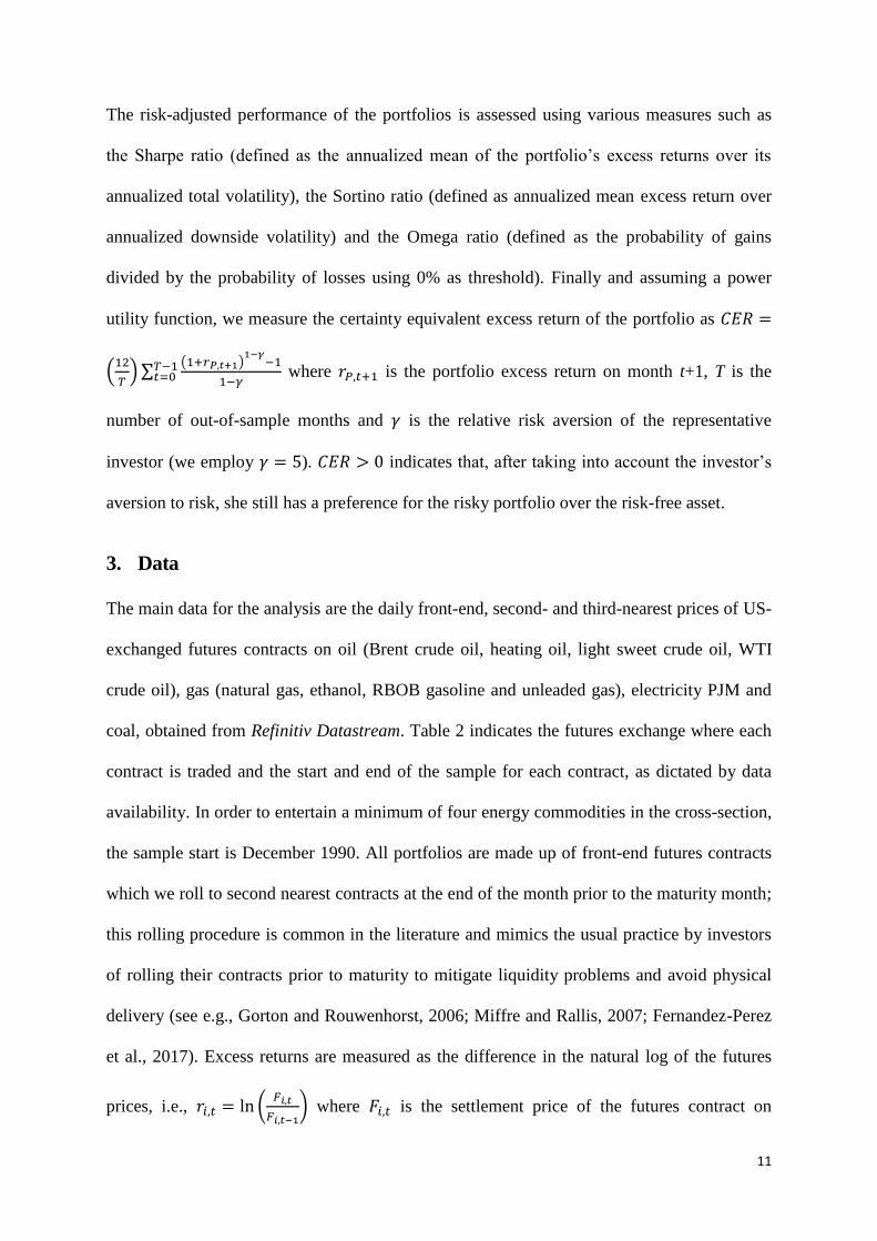
The risk-adjusted performance of the portfolios is assessed using various measures such as
the Sharpe ratio (defined as the annualized mean of the portfolio’s excess returns over its
annualized total volatility), the Sortino ratio (defined as annualized mean excess return over
annualized downside volatility) and the Omega ratio (defined as the probability of gains
divided by the probability of losses using 0% as threshold). Finally and assuming a power
utility function, we measure the certainty equivalent excess return of the portfolio as
where is the portfolio excess return on month t+1, T is the
number of out-of-sample months and is the relative risk aversion of the representative
investor (we employ ). indicates that, after taking into account the investor’s
aversion to risk, she still has a preference for the risky portfolio over the risk-free asset.
3. Data
The main data for the analysis are the daily front-end, second- and third-nearest prices of US-
exchanged futures contracts on oil (Brent crude oil, heating oil, light sweet crude oil, WTI
crude oil), gas (natural gas, ethanol, RBOB gasoline and unleaded gas), electricity PJM and
coal, obtained from Refinitiv Datastream. Table 2 indicates the futures exchange where each
contract is traded and the start and end of the sample for each contract, as dictated by data
availability. In order to entertain a minimum of four energy commodities in the cross-section,
the sample start is December 1990. All portfolios are made up of front-end futures contracts
which we roll to second nearest contracts at the end of the month prior to the maturity month;
this rolling procedure is common in the literature and mimics the usual practice by investors
of rolling their contracts prior to maturity to mitigate liquidity problems and avoid physical
delivery (see e.g., Gorton and Rouwenhorst, 2006; Miffre and Rallis, 2007; Fernandez-Perez
et al., 2017). Excess returns are measured as the difference in the natural log of the futures
prices, i.e.,
where is the settlement price of the futures contract on

12
commodity i at time t. It can be shown that the excess return represents the total return of
a fully-collateralized futures position in excess of the risk-free rate (Erb and Harvey, 2006).
We also obtain from Refinitiv Datastream the daily traded volume of each contract and from
the Commodity Futures Trading Commission (CFTC) archive the weekly positions of large
commercial (hedgers) and non-commercial (speculators) participants as provided in the
Futures-Only Legacy Commitments of Traders (CoT) report from September 30, 1992
onwards.8 These weekly positions of futures traders are used to calculate the hedging pressure
and speculative pressure signals for each commodity as defined in Table 1. In order to make
the comparison of performance across strategies as informative as possible, it is focused on
the period July 2001 to March 2019 that is common to all (single-style and integrated)
strategies.
Table 2, Panel A presents summary statistics for the excess returns of the futures contracts.
The annualized mean excess return averaged across contracts merely stands at -3.06% a year.
The risk profile of the contracts is high with, for example, annualized standard deviation and
maximum drawdown that average 35.2% and -77% across assets. With the noticeable
exception of ethanol and corroborating the evidence from 12 individual commodity futures
markets of e.g., Erb and Harvey (2006), the results confirm the poor risk-adjusted
performance of energy futures contracts when treated as stand-alone investments. Indirectly,
8 Although the CoT dataset is widely used (e.g., Bessembinder, 1992; Hirshleifer, 1988; Basu
and Miffre, 2013; Kang et al., 2020), it has limitations. The classification of traders into
commercials (hedgers) and non-commercials (speculators) is based on information provided
by the traders themselves; large traders ought to declare the nature of their positions and any
association with the physical market activities. One cannot rule out that some speculators
might self-classify their activity as commercial to circumvent position limits, although the
CFTC supervises the declarations seeking to correct any misclassifications. Moreover, futures
market pundits have criticized the CFTC taxonomy of swap dealers (such as index trackers)
as commercials. Swap dealers usually have no position in the physical commodity but instead
their hedging is associated with over-the-counter (OTC) derivative positions. For further
discussion see e.g., Ederington and Lee (2002) and Irwin and Sanders (2012).

13
this finding serves to highlight the need to adopt a long-short signal-sorted portfolio
construction approach in energy markets, which is precisely the methodology that this paper
advocates.
[Insert Table 2 around here]
Table 2, Panel B reports averages for the sorting signals. As expected, we note a propensity
for the futures with higher annualized mean returns (e.g., ethanol) to present backwardated
characteristics such as higher roll-yields, higher hedging pressure (HP), higher speculative
pressure (SP) and higher momentum signals. Vice versa, futures with lower annualized mean
returns (e.g., natural gas) show signs of contango as demonstrated by lower roll-yields, lower
HP, lower SP and lower momentum signals. This provides preliminary evidence that the
signals employed are key to the pricing of energy contracts and thus potentially useful for
asset allocation. The descriptive statistics confirm the stylized fact of the energy sector that
crude oil futures by far lead the pack as the most liquid contracts. This may have some effect
on the performance of the strategies via transaction costs (TC), which we investigate below.
For the TC analysis, we will employ information on the contract multiplier and minimum tick
size per commodity futures contract, as shown in the Panel C of Table 2, from Refinitiv
Datastream.9
4. Empirical Results
4.1. Single-style portfolios
9 The contract multiplier ( also called contract size) is the total number of commodity
units specified in each futures contract. The minimum tick ( ) is the minimum price
fluctuation of the futures contract per unit of the underlying commodity. Both are set by the
corresponding futures exchange (e.g., NYMEX for light sweet crude oil) and vary by
contract. For instance, a light sweet crude oil futures contract commits the holder to buy or
sell 1,000 barrels of oil so the contract multiplier is 1,000 while the minimum tick is $0.01 per
barrel. Accordingly, the dollar value of one tick of a light sweet futures contract is .
14
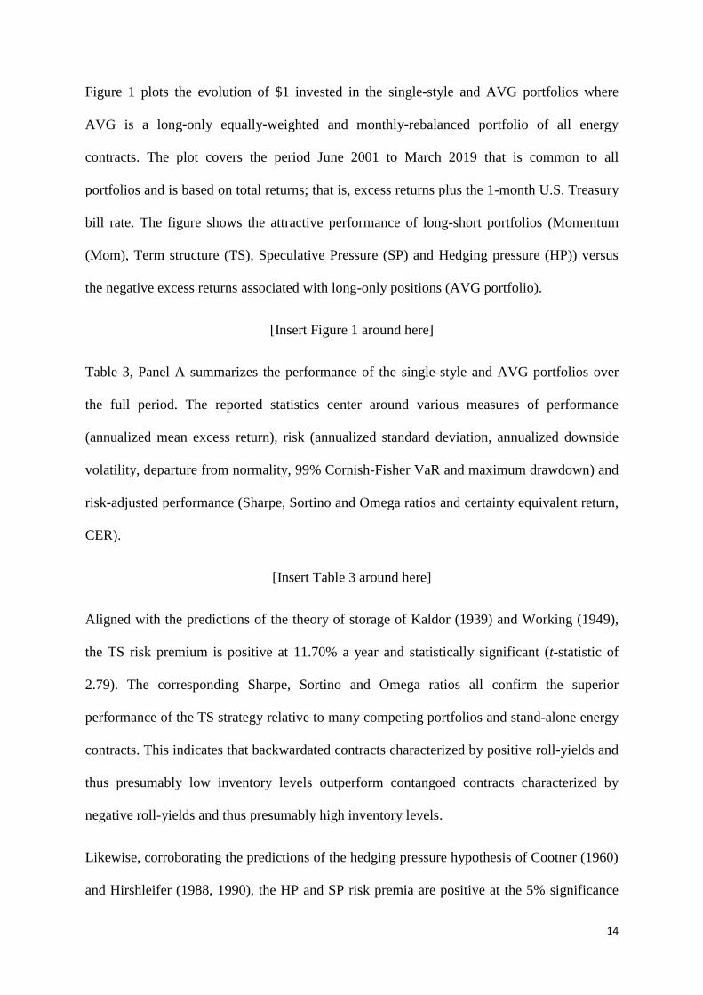
Figure 1 plots the evolution of $1 invested in the single-style and AVG portfolios where
AVG is a long-only equally-weighted and monthly-rebalanced portfolio of all energy
contracts. The plot covers the period June 2001 to March 2019 that is common to all
portfolios and is based on total returns; that is, excess returns plus the 1-month U.S. Treasury
bill rate. The figure shows the attractive performance of long-short portfolios (Momentum
(Mom), Term structure (TS), Speculative Pressure (SP) and Hedging pressure (HP)) versus
the negative excess returns associated with long-only positions (AVG portfolio).
[Insert Figure 1 around here]
Table 3, Panel A summarizes the performance of the single-style and AVG portfolios over
the full period. The reported statistics center around various measures of performance
(annualized mean excess return), risk (annualized standard deviation, annualized downside
volatility, departure from normality, 99% Cornish-Fisher VaR and maximum drawdown) and
risk-adjusted performance (Sharpe, Sortino and Omega ratios and certainty equivalent return,
CER).
[Insert Table 3 around here]
Aligned with the predictions of the theory of storage of Kaldor (1939) and Working (1949),
the TS risk premium is positive at 11.70% a year and statistically significant (t-statistic of
2.79). The corresponding Sharpe, Sortino and Omega ratios all confirm the superior
performance of the TS strategy relative to many competing portfolios and stand-alone energy
contracts. This indicates that backwardated contracts characterized by positive roll-yields and
thus presumably low inventory levels outperform contangoed contracts characterized by
negative roll-yields and thus presumably high inventory levels.
Likewise, corroborating the predictions of the hedging pressure hypothesis of Cootner (1960)
and Hirshleifer (1988, 1990), the HP and SP risk premia are positive at the 5% significance

15
level or better, ranging from 7.58% a year for HP (t-statistic of 2.22) to 8.16% a year for SP
(t-statistic of 2.79).10
The corresponding Sharpe ratios stand at 0.57 and 0.65, respectively.
This shows that backwardated energy futures contracts characterized by net short hedgers
tend to appreciate in value to entice net long speculation, while contangoed energy futures
contracts characterized by net long hedgers tend to depreciate in value to entice net short
speculation. To state this differently, hedgers in energy futures markets are willing to pay a
premium of 7.58% a year to invite speculators to take on the price risk that they would like to
get rid of. Speculators in turn demand a similarly sized premium of 8.16% as reward for the
risk born.
The momentum portfolio generates a positive mean excess return equal to 13.28% a year
with a t-statistic of 3.53 or a Sharpe ratio of 0.75. This remarkable performance reflects the
fact that the momentum portfolio, like the TS, HP and SP portfolios, captures the phases of
backwardation and contango (Miffre and Rallis, 2007; Gorton et al., 2013). The value
strategy earns an interesting Sharpe ratio at 0.32; yet, its mean excess return is statistically
insignificant and its CER is negative at -3.19% a year. The risk premia associated with
liquidity and skewness are insignificant, both statistically and economically.
The Keynesian hypothesis assumes that futures markets are normally backwardated. In the
setting of Keynes (1930), energy producers are long the physical asset and willing to take a
short hedge to reduce their exposure to potentially declining oil prices. To get rid of their
10 The risk premia captured by the HP and SP strategies needs not be identical since the
hedgers and speculators’ open positions used to construct the underlying signals, obtained
from the Commitment of Traders (CoT) report of the Commodity Futures Trading
Commission (CFTC), do not represent the total of open positions but only those of large
traders that ought to report their positions to the CFTC (referred to as reportables). If large
traders covered the 100% of the open interest instead, the HP and SP signal would be
perfectly positively correlated because for every long position there is a matching short
position, and the HP and SP premia would then be identical as the commodities ranking (by
the HP and SP signals) would coincide.

16
price risk, they need to entice speculators to take the long side of the futures market and thus,
futures prices have to rise with maturity. In other words, if the normal backwardation theory
holds, long speculators shall earn a positive risk premium as compensation for bearing
hedgers’ price risk. In our setting, the AVG portfolio earns a mean excess return of -2.20% a
year (t-statistic of -0.29) or a Sharpe ratio at -0.08, a poor performance that is reminiscent of
that of individual energy contracts (c.f., Table 2). This poor performance reveals that the
actual pricing of energy futures contracts does not support the normal backwardation theory
of Keynes (1930). Instead of long-only portfolios, investors ought to take simultaneous long
and short positions in the cross-section of energy futures contracts to capture a sizeable risk
premium.
Table 3, Panel B reports the Sharpe ratios of the long-short single-style and AVG portfolios
over four non-overlapping subsamples of equal size, alongside relative rankings of
performance ranging from 1 (for the best performing strategy) to 8 (for the worst performing
strategy). We note some instability in the relative rankings over time. For example, the HP
and value strategies rank both amongst the worst and best strategies depending on the sub-
sample considered. This instability in relative rankings motivates style integration as a way to
diversify risk by preempting the difficult choice of one signal over another one.
Table 4 provides pairwise Pearson correlations across the excess returns of the K single-sort
styles. The excess returns of the TS, HP, SP and Mom portfolios have relatively high
correlations ranging from 0.25 to 0.79 with an average at 0.44; this is expected as these
individual styles are all deemed to capture the fundamentals of backwardation and contango.
The average correlations across individual-style portfolio returns is, however, low at 0.09
suggesting that integration could help achieve diversification benefits. The value portfolio,
which is contrarian in nature, and the liquidity portfolio present negative return correlation

17
with the other portfolios. This low dependence in the excess returns of the single-style
portfolios motivates an integrated portfolio approach as a way of managing risk.
[Insert Table 4 around here]
4.2. Integrated portfolios
Figure 2 plots the future value of $1 invested in June 2001 in various fully-collateralized
integrated portfolios. It provides preliminary evidence of the benefits of integration and of the
possible superiority of the naïve EWI approach over the sophisticated OI and VTI
alternatives. Table 5 complements this analysis by summarizing the performance of the
integrated portfolios over the whole sample (Panel A) and over four non-overlapping
subsamples of equal size (Panel B). Aligned with the first impression provided by Figure 2,
Table 5 shows that integration works: all integration techniques deliver positive mean excess
returns that are significant at the 1% level. The corresponding Sharpe ratios range from 0.74
to 0.90 and are thus at worst equal to those obtained in Table 3 for the single-style portfolios.
This serves to highlight the benefits of integration: by relying on a composite signal that
aggregates information from various styles, the investor predicts more reliably subsequent
price changes and is thus better able to capture the risk premium present in energy futures
markets.
[Insert Table 5 and Figure 2 around here]
EWI stands out among all the integration methods deployed with the highest mean excess
return at 12.4% a year, the highest Sharpe and Omega ratios at 0.90 and 2.04, respectively,
the second highest Sortino ratio at 1.28 and the highest CER at 7.36% a year. The efficacy of
EWI to capture risk premia may be due to the fact that, unlike OI and VTI, it incurs no
estimation uncertainty (the style-weight parameter is preset) and also it sidesteps

18
representativeness heuristic bias (it does not rely on the persistence of the performance of the
single styles).11
To assess the statistical superiority of EWI relative to OI and VTI, we calculate the Opdyke
(2007) p-value for the null hypothesis versus where j
denotes an integrated portfolio other than EWI. In order to account for higher order moments
of the return distribution, we also test the null hypothesis versus
. The p-values, reported in Table 5, Panel A, fail to reject the null
hypothesis at conventional levels.12
Statistically, the Sharpe ratio and CER of the EWI
portfolio are at least as attractive as those of the OI and VTI portfolios.
Table 5, Panel B presents the Sharpe ratios of each integrated portfolio over four consecutive
subsamples of equal size. It reports in parentheses the rank assigned to a given integrated
portfolio in relation to the other 13 portfolios (AVG, 7 single-style portfolios and 5
alternative integrated portfolios). A rank of 1 (14) is assigned to the strategy with the highest
(lowest) Sharpe ratio over a given sub-sample. These period-specific ranks are subsequently
averaged across periods. The lower the average rank, the better the performance of the
strategy under review. With an average rank at 3.5, EWI beats all competing integration
approaches. Unreported results show that EWI also beats AVG and the single-style strategies
of Table 3.
5. Robustness Tests
11 Tversky and Kahneman (1974) define representative heuristic as a behavioral tendency to
wrongly overstate the importance of an observation. In the present context, the bias amounts
to thinking that the best (worst) styles will keep outperforming (underperforming).
12 We use the bootstrap method of Politis and Romano (1994) to test the statistical
significance of the difference in CER. The p-values are obtained by resampling blocks of
random length from the actual time-series { using B=10,000 bootstrapped excess
returns
of length T=213. The block-length is a geometrically distributed variable
with expected value for p=0.2. Similar results were obtained with p=0.5.

19
For the sake of completeness, we subject our key findings on the presence of an energy
futures risk premium and on the superior performance of EWI to various robustness tests.
5.1. Turnover and transaction costs
Trading intensity erodes performance and could even potentially wipe out the profits of
seemingly lucrative strategies. It is thus important to measure the turnover of the single-style
and integrated portfolios; higher turnover indeed comes hand-in-hand with worse
performance net of reasonable transaction costs. Bearing this in mind, we define the turnover
of strategy j, , as the time average of all the trades incurred
(4)
where is the weight assigned to the ith energy contract by the jth portfolio at time t (in
the case of a single-style portfolio, ), is the weight of the
ith contract before the next rebalancing at t+1, and is the excess return of the ith energy
contract from to . Thus measures the natural evolution of the weights within the
month as driven by the performance of the contract. Theoretically, the turnover measure
ranges from 0 (should no trading occurs) to 2 (should all the long positions be reversed every
month and likewise for the shorts). The results, reported in Table 6, show that with turnover
ranging from 0.0972 (HP) to 0.3915 (Value), the strategies considered are not highly trading
intensive and thus, it is unlikely that transaction costs will wipe out performance.
We then calculate the excess returns of each strategy after transaction costs as follows
(5)
with TC denoting a round-trip trading cost. While relatively patient energy futures traders
willing to stagger the allocation of a $1 million wealth into futures positions within a 60-
minute window are prepared to pay up TCs of up to 6.7 b.p., demands for more immediate

20
execution raise the transaction costs to 20 b.p. (Marshall et al. 2012). Bearing their point in
mind, it might be worth it to analyze whether the need for immediacy could harm
performance so much that it deters traders from implementing the trades. The results,
reported in Table 6, show that inferences regarding the presence of an energy risk premium
and the superiority of EWI hold after transaction costs. For example, the risk premium based
on the phases of backwardation and contango are still significant at the 5% level or better
after accounting for transaction costs. EWI still offers the highest net mean excess returns and
the highest net Sharpe ratio.
Finally, we perform a breakeven analysis that gives the transaction costs required for the
mean excess return of a given strategy to be zero; namely, in the following
equation
, (6)
where following Szakmary et al. (2010) and Paschke et al. (2020) inter alia, heterogeneity in
the transaction costs across energy futures contract at time t is allowed with defined as
, (7)
which formalizes the wisdom that commodity futures trading costs are a function of the: a)
minimum tick of the ith contract ( ), b) contract size or contract multiplier ( ), c) time
t settlement price ( ), d) a brokerage fee of roughly $10 (Pashke et al., 2020), and e) a
parameter that measures the number of times the dollar value of one tick is to be paid for
the price impact of trading to wipe out the gross returns of the strategy. We solve Equation
(6) for k, and calculate using Equation (7) with the commodity-specific information of
the minimum tick and contract multiplier reported in Panel C of Table 2. The last column of
Table 6 reports the average break-even cost in b.p. across time and energy
commodities . These estimates suggest that the trading costs needed for the profits

21
of Tables 3 and 5 to be wiped out are extremely large. Specifically, it would require costs that
are 56 times and 19 times the 6.7 b.p. and 20 b.p. estimates of Marshall et al. (2012),
respectively, to wipe out the attractive gross profits of the TS, HP, SP and Mom strategies
(Table 3) and those of the integrated strategies (Table 5). We can safely conclude that the risk
premia extracted by the portfolio strategies proposed are not an artefact of transaction costs.13
[Insert Table 6 around here]
5.2. Alternative specifications of the weighting schemes
Thus far, we followed the literature (see e.g., Asness et al., 2013) in forming balanced long-
short portfolios that invest 50% of the investor’s mandate in long positions and the remainder
50% in short positions. This could result in long positions being taken at time t in, for
example, contangoed contracts (shall most or all contracts be in contango) and short positions
being taken in, for example, backwardated contracts (shall most or all contracts be in
backwardation). We test whether such occurrence impacts our general conclusions on
performance by using as asset allocation criterion the actual signal k of commodity i at time t,
(e.g., the roll-yield), instead of . We then buy the
energy futures contracts whose prices are expected to rise (allocation weights ) and
short the energy futures contracts whose prices are expected to drop (allocation weights
) such that with denoting the size of the entire cross-section. Since
in this case we use directly the (non-standardized) signal which is therefore not
centered, the implication is that we no longer have a balanced portfolio, namely
where
and We invest
in each contract i at portfolio formation time t so that the mandate
13 The less refined approach that consists of solving the Equation (5), , directly for
gives similar results which are unreported but available from the authors upon request.

22
is fully collateralized ( . Therefore, at each month end (time t) over the sample
period this asset allocation could be 100% long (when ), 100% short (when )
or any long-short in between (when and ). Proceeding likewise for all signals,
we end up with six portfolios sorted on single styles. We omit the liquidity-sorted portfolio
whose signal is by definition always negative. The style-integrated portfolios are formed as
before but using the non-standardized signals. Table 7, Panel A, presents summary statistics
for the performance of the modified portfolios. The risk premia captured by these portfolios
is notably inferior to that stemming from our portfolios based on standardized signals,
; this standardized-signal approach has become typical since the
seminal paper of Brandt et al. (2009). For example, the mean excess returns of the portfolios
based on the non-standardized signals is 4% p.a. on average (Table 7, Panel A) versus 8.58%
p.a. for the portfolios with weights given by the standardized signals (Tables 3 and 5). The
corresponding average Sharpe ratios are 0.18 and 0.61, respectively.
[Insert Table 7 around here]
We attribute the notably smaller risk premia captured by the long-short portfolios based on
non-standardized signals to the fact that these portfolios are not market neutral, i.e., they do
not capture a signal-based risk premium that is actually immune to market movements. To
show this, we regress the excess returns of the portfolios sorted on non-standardized signals
onto the excess returns of the AVG portfolio. We do likewise for the excess returns of the
portfolios sorted on standardized signals. Table 7, Panels B and C present the estimated
parameters and goodness-of-fit statistics of these regressions. As anticipated, the portfolios
based on non-standardized signals are not market neutral: the AVG slope in Table 7, Panel B
is significant at the 5% level or better for all the single-style portfolios but momentum with
an average adjusted-R2 across single-styles of 0.21; it is also significant at the 10% level for
most of the style-integrated portfolios. The intercept or alpha (performance over and above
23
the market) is insignificant for all single- and style-integrated portfolios. The smaller risk
premia stemming from the portfolios in Panel A is therefore driven by the poor performance
of AVG (Table 3). Likewise, the style-integrated portfolios based on non-standardized
signals capture a much smaller risk premia than the corresponding style-integrated portfolios
based on standardized signals. In sharp contrast, the portfolios sorted on standardized signals
(Table 7, Panel C) are market neutral: the slope coefficients are insignificant for all the
single-style and style-integrated portfolios with a negligible average adjusted-R2. The alphas
are significant at the 5% level or better for all the single-style portfolios but value and
skewness, and the style-integrated portfolios. Thus, the portfolios based on standardized
signals capture a larger signal-based risk premia because they are immune to general energy
futures market movements.
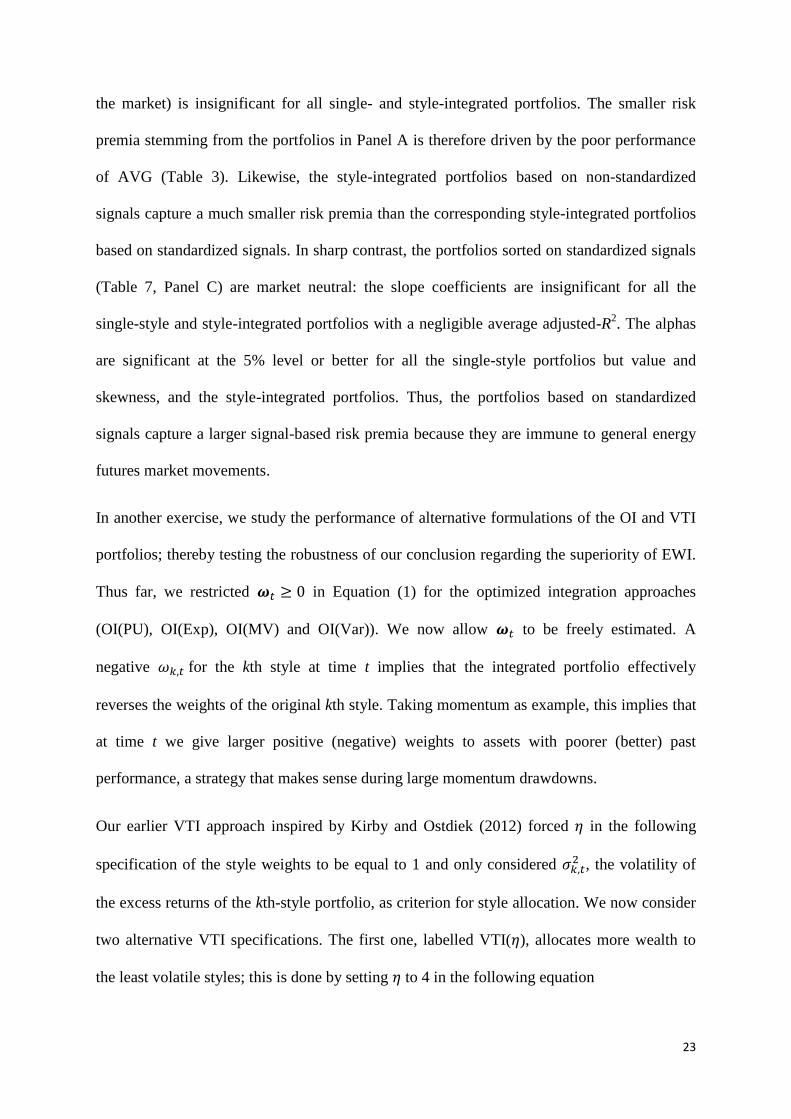
In another exercise, we study the performance of alternative formulations of the OI and VTI
portfolios; thereby testing the robustness of our conclusion regarding the superiority of EWI.
Thus far, we restricted in Equation (1) for the optimized integration approaches
(OI(PU), OI(Exp), OI(MV) and OI(Var)). We now allow to be freely estimated. A
negative for the kth style at time t implies that the integrated portfolio effectively
reverses the weights of the original kth style. Taking momentum as example, this implies that
at time t we give larger positive (negative) weights to assets with poorer (better) past
performance, a strategy that makes sense during large momentum drawdowns.
Our earlier VTI approach inspired by Kirby and Ostdiek (2012) forced in the following
specification of the style weights to be equal to 1 and only considered , the volatility of
the excess returns of the kth-style portfolio, as criterion for style allocation. We now consider
two alternative VTI specifications. The first one, labelled VTI( ), allocates more wealth to
the least volatile styles; this is done by setting to 4 in the following equation

24
(8)
while the second specification, labelled VTI( ), considers both performance and volatility as
criteria for style allocation as formalized by
(9)
where and is the mean excess return of the kth style. A 60-month
window is used to estimate and in all these alternative formulations of the OI and VTI
portfolios. The results in Table 8 reveal that none of these alternatives outperforms EWI.
Thus, the style-integration that ascribes equal weights to all signals is confirmed as the best
approach.
[Insert Table 8 around here]
5.3. Data mining
Our conclusion thus far is that EWI outperforms the 19 alternative strategies considered: the
AVG portfolio, the 7 single-style (SS) strategies, , the 8 OI specifications
and the 3 VTI specifications, (i.e., the integrated portfolios reported in Tables 5 and
8). Is this a result of data snooping?14
We use the Superior Predictive Ability test of Hansen
(2005) based on Sharpe ratio differences to address this issue.
We treat EWI as benchmark and compare the Sharpe ratios of the 19 underperforming
portfolios to that of EWI. Let SRm denote the Sharpe ratio of strategy
and the Sharpe ratio of EWI. Relative
performance is measured by the Sharpe ratios differential, . The
14 Employing the same dataset to assess the performance of many investment strategies can
trigger false discoveries; this is the data snooping issue as it is understood by practitioners.
25
expected “loss” of the mth strategy relative to the benchmark is therefore
. Strategy m is better in terms of Sharpe ratio than the benchmark (EWI) if and only if
. The null hypothesis is that the best of the strategies does not obtain a
superior Sharpe ratio than the Sharpe ratio of the EWI benchmark; i.e.,
.
Using the bootstrap method of Politis and Romano (1994), we obtain 10,000 bootstrap time-
series of excess returns for the EWI benchmark and for the 19 underperforming portfolios by
pooling random blocks from the original time-series of excess returns. The length of each
sample block follows a geometric distribution with expected value 1/p with p
Subsequently, we obtain 10,000 pseudo values for for each of the
strategies. The p-values of 0.9772 (p=0.2) and
0.9725 (p=0.5) clearly show that the null hypothesis cannot be rejected. Altogether, we
conclude that the superiority of the EWI portfolio cannot be attributed to data snooping.
5.4. Subsample analysis
Finally, we test whether the results are sample specific by re-evaluating the performance of
the single and integrated energy portfolios over different sub-periods defined as follows: i)
high versus low volatility in energy futures markets where the volatility is modelled by fitting
a GARCH(1,1) model to the excess returns of AVG15
, ii) pre and post the financialization of
commodity futures markets roughly dated January 2006 (Stoll and Whaley, 2010), iii) in
periods of recession and expansion according to the NBER-dated business cycle phases, and
iv) over the bust of the 2008 oil price bubble (July 2008 – February 2009)16
versus the rest of
15 The threshold to separate the high and low volatility regimes is defined as the average of
the annualized fitted volatility estimated at 27.6%.
16 The bust of the 2008 oil price bubble had a remarkable effect in energy futures. For
instance, the AVG portfolio lost 13.47% a month from July 2008 to February 2009.

26
the sample. Table 9 reports the Sharpe ratios of the single-style strategies in Panel A and
those of the integrated strategies in Panel B. The single-style risk premia based on
backwardation and contango are often robust to the sub-sample considered; yet, they are
found to be stronger in periods of expansion and since the financialization of commodity
futures markets. Over the period spanning the bust of the 2008 oil price bubble (July 2008 to
February 2009), all the long-short portfolios present positive Sharpe ratios ranging from 0.18
(Skewness) to 3.34 (OI(Var)).17
Most importantly, the integrated portfolios deliver positive
Sharpe ratios in all sub-samples; the conclusion holds irrespective of the integration approach
considered. Altogether, the table further highlights the benefits of style-integrated long-short
portfolios as they are able to capture sizeable energy risk premia irrespective of market
conditions.
[Insert Table 9 around here]
6. Conclusions
The theory of storage of Kaldor (1939), Working (1949) and Brennan (1958) and the hedging
pressure hypothesis of Cootner (1960) and Hirshleifer (1988, 1990) suggest that the state of
the commodity futures market, backwardation versus contango, contains predictive ability for
commodity futures prices. This article examines the ability to extract energy risk premia of
long-short portfolios formed according to various futures contract characteristics that proxy
the backwardation and contango dynamics such as the roll-yield, hedging pressure and
17 A reassuring finding is that over the bust period of the oil bubble the long-short portfolios
formed according to the HP and SP signals motivated by the hedging pressure hypothesis still
capture sizeable risk premia. For instance, the mean excess return of the SP portfolio is
2.17% per month (26.04% p.a.) and a Sharpe ratio of 1.10 suggesting that the risk transfer
mechanism was at play also during this challenging period – namely, speculators earned a
significant premium of 2.17% per month (26.04% p.a.) for shouldering the price risk that
hedgers sought to avoid. The results of a similar exercise over January 2008 to February 2009
which spans the boom and bust components of the bubble are qualitatively similar.

27
momentum inter alia. The energy risk premia thus captured ranges from a sizeable 7.58% to
13.28% a year with Sharpe ratios of 0.65 to 0.75. Jointly exploiting the backwardation versus
contango signals (and other signals such as liquidity, value and skewness) into a long-short
integrated portfolio increases the Sharpe ratio further to 0.90. The findings hold after
accounting for trading costs, alternative designs of the integrated portfolio, data snooping
tests and economic sub-periods.
Our empirical findings serve to endorse the theory of storage and hedging pressure
hypothesis in the specific energy futures sector. From a regulatory perspective, the ability to
extract a significant energy risk premium through a long-short portfolio formed according to
the hedging pressure characteristic reveals that an effective risk transfer mechanism from
hedgers to speculators is at play in the energy futures sector. This empirical finding indirectly
suggests that calls for further regulation of speculative activity are unwarranted at this stage.
From a practitioners’ perspective, our paper proposes long-short strategies that can inspire the
design of energy-based smart-beta index products and thus are relevant for asset management
practice.
28
References
Alquist, R. and Kilian, L., 2010, What do we learn from the price of crude oil futures?
Journal of Applied Econometrics 25, 539-573
Amaya, D., Christoffersen, P., Jacobs, K., and Vasquez, A., 2015. Does realized skewness
predict the cross-section of equity returns? Journal of Financial Economics 118, 135-167
Amihud, Y., Mendelson, H., and Lauterbach, B., 1997. Market microstructure and securities
values: evidence from the Tel Aviv exchange. Journal of Financial Economics 45, 365-
390
Amihud, Y., Mendelson, H., and Pedersen, L., 2005, Liquidity and asset prices. Foundations
and Trends in Finance 1, 269-364
Asness, C., Moskowitz, T., and Pedersen, L., 2013. Value and momentum everywhere.
Journal of Finance 68, 929-985
Barroso, P., and Santa-Clara, P., 2015. Beyond the carry trade: Optimal currency portfolios.
Journal of Financial and Quantitative Analysis 50, 1037-1056
Basu, D., and Miffre, J., 2013. Capturing the risk premium of commodity futures: The role of
hedging pressure. Journal of Banking and Finance 37, 2652-2664
Bessembinder, H., 1992. Systematic risk, hedging pressure, and risk premiums in futures
markets. Review of Financial Studies 5, 637-667
Bessembinder, H., Lemmon, M.L., 2002. Equilibrium pricing and optimal hedging in
electricity forward markets. Journal of Finance 57, 1347-1382
Boons, M., and Prado, M., 2019. Basis momentum, Journal of Finance 74, 239-279
Brandt, M., Santa-Clara, P., and Valkanov, R., 2009. Parametric portfolio policies: Exploiting
characteristics in the cross-section of equity returns. Review of Financial Studies 22,
3444-3447
Brennan, M., 1958. The supply of storage. American Economic Review 48, 50-72
Byun, S.-J., 2017. Speculation in commodity futures Markets, inventories and the price of
crude oil. Energy Journal 38, 93-113
Chiang, I.-H., 2016. Skewness and coskewness in bond returns. Journal of Financial Research
39, 145-178
Cho, D., and Douglas, G., 1990. The supply of storage in energy futures markets. Journal of
Futures Markets 10, 611-621
Cootner, P., 1960. Returns to speculators: Telser vs. Keynes. Journal of Political Economy
68, 396-404
DeMiguel, V., Martín-Utrera, A., Nogales, F.J., and Uppal, R., 2020. A transaction-cost
perspective on the multitude of firm characteristics. Review of Financial Studies 33,
2180-2222
Dewally, M., Ederington, L., and Fernando, C., 2013. Determinants of trader profits in
commodity futures markets. Review of Financial Studies 26, 2648-2683

29
Ederington, L., Fernando, C., Holland, K., Lee, T., and Linn, S., 2020, Dynamics of
arbitrage. Journal of Financial and Quantitative Analysis, 1-31
Ederington, L., and Lee J. H., 2002. Who trades futures and how: Evidence from the heating
oil futures market. Journal of Business, 75, 353-373
Erb, C., and Harvey, C., 2006. The strategic and tactical value of commodity futures.
Financial Analysts Journal 62, 69-97
Fama, E., and French, K., 1987. Commodity futures prices: Some evidence on forecast
power, premiums, and the theory of storage. Journal of Business 60, 55-73
Fattouh, B., Kilian, L., and Mahadeva, L., 2013.The role of speculation in oil markets: What
have we learned so far? Energy Journal 34, 7-33
Fernandez-Perez, A., Frijns, B., Fuertes, A.-M., and Miffre, J., 2018. The skewness of
commodity futures returns. Journal of Banking and Finance 86, 143-158
Fernandez-Perez, A., Fuertes, A.-M., and Miffre, J., 2017. Commodity markets, long-run
predictability and intertemporal pricing. Review of Finance 21, 1159-1188
Fernandez-Perez, A., Fuertes, A.-M., and Miffre, J., 2019. A comprehensive appraisal of
style-integration methods. Journal of Banking and Finance 105, 134-150
Fischer M., and Gallmeyer. M.F., 2016. Heuristic portfolio trading rules with capital gain
taxes. Journal of Financial Economics 119, 611-625
Fitzgibbons, S., Friedman, J., Pomorski, L., and Serban, L., 2016. Long-only style investing:
Don’t just mix, integrate. AQR Capital Management white paper June 2016
Furió, D., and Meneu, V., 2010. Expectations and forward risk Premium in the Spanish
deregulated power market. Energy Policy, 38, 784 -793.
Furió, D., and Torró, H., 2020. Optimal hedging under biased energy futures markets. Energy
Economics, 88, 104750
Ghysels, E., Plazzi, A., and Valkanov, R., 2016. Why invest in emerging markets? The role of
conditional return asymmetry. Journal of Finance 71, 2145-2192
Gorton, G., and Rouwenhorst, G., 2006. Facts and fantasies about commodity futures.
Financial Analysts Journal 62, 47-68
Gorton, G., Hayashi, F., and Rouwenhorst, G., 2013. The fundamentals of commodity futures
returns, Review of Finance 17, 35-105
Hansen, P.R., 2005. A test for superior predictive ability. Journal of Business and Economic
Statistics 23, 365-380
Hirshleifer, D., 1988. Residual risk, trading costs, and commodity futures risk premia.
Review of Financial Studies 1, 173-193
Hirshleifer, D., 1990. Hedging pressure and future price movements in a general equilibrium
model. Econometrica 58, 441-28.
Irwin, S.H., and Sanders, D.R., 2012. Testing the Masters Hypothesis in commodity futures
markets. Energy Economics 34, 256-269
Kaldor, N., 1939. Speculation and economic stability. Review of Economic Studies 7, 1-27

30
Kang, W., Rouwenhorst, K. G., and Tang, K., 2020. A tale of two premiums: the role of
hedgers and speculators in commodity futures markets. Journal of Finance 75, 377-417
Keynes, J., 1930. Treatise on Money (Macmillan, London)
Kirby, C., and Ostdiek, B., 2012. It’s all in the timing: Simple active portfolio strategies that
outperform naïve diversification. Journal of Financial and Quantitative Analysis 47, 437-
467
Koijen, R., Moskowitz, T., Pedersen, L., and Vrugt, E., 2018. Carry. Journal of Financial
Economics 127, 197-225
Kroencke, T., Schindler, F., and Schrimpf, A., 2014. International diversification benefits
with foreign exchange investment styles. Review of Finance 18, 1847-1883
Longstaff, F.A., and Wang, A.W., 2004. Electricity forward prices: a high-frequency
empirical analysis. Journal of Finance 59, 1877-1900
Lucia, J., and Torró, H., 2011. On the risk premium in Nordic electricity futures prices.
International Review of Economics and Finance 20, 750-763
Marshall, B. R., Nguyen, N. H. and Visaltanachoti, N., 2012. Commodity liquidity
measurement and transaction costs. Review of Financial Studies 25, 599-638
Martínez, B., and Torró, H., 2018. Analysis of risk premium in UK natural gas futures.
International Review of Economics and Finance 58, 621-636
Miffre, J., and Rallis, G., 2007. Momentum strategies in commodity futures markets. Journal
of Banking and Finance 31, 6, 1863-1886
Opdyke J.D., 2007. Comparing Sharpe ratios: So, where are the p-values? Journal of Asset
Management 8, 308-336
Paschke, R., Prokopczuk, M., and Simen, C. W., 2020. Curve momentum. Journal of
Banking and Finance, 113, 105718
Politis, D.N., and Romano, J.P., 1994. The stationary bootstrap. Journal of the American
Statistical Association 89, 1303-1313
Pindyck, R., 2001. The dynamics of commodity spot and futures markets: A primer. Energy
Journal 22, 1-29
Sanders, D., Boris, K., and Manfredo, M., 2004. Hedgers, funds, and small speculators in the
energy futures markets: An analysis of the CFTC’s commitments of traders reports.
Energy Economics 26, 425-445
Serletis, A., and Hulleman, V., 1994. Business cycles and the behavior of energy prices.
Energy Journal 15, 125-134
Stoll, H., and Whaley, R. 2010. Commodity index investing and commodity futures prices.
Journal of Applied Finance 20, 7-46
Szakmary, A.C., Shen, Q., and Sharma, S.C., 2010. Trend-following trading strategies in
commodity futures: A re-examination. Journal of Banking and Finance 34, 409-426

31
Szymanowska, M., De Roon, F., Nijman, T., and Van Den Goorbergh, R., 2014. An anatomy
of commodity futures risk premia. Journal of Finance 69, 453-482
Tang, K. and W., Xiong, 2012, Index investment and financialization of commodities.
Financial Analysts Journal 68, 54-74
Till, H., 2009, Has there been excessive speculation in the US oil futures markets? EDHEC-
Risk Institute research paper.
Tversky, A., and Kahneman, D., 1974. Judgments under uncertainty: Heuristics and biases.
Science, 185, 1124-1131
Working, H., 1949. The theory of price of storage. American Economic Review 39, 1254-
1262

32
Table 1. Individual investment styles.
The first column lists the style, the second and third columns report the signal or characteristic of the underlying asset used to construct the long-
short portfolios (a higher indicates a higher expectation of a futures price increase), and the last column summarizes the background
literature.
Style Signal References
Panel A: Styles that capture the fundamentals of backwardation and contango
Term structure
(TS)
Roll yield or basis defined as difference in daily log prices of front-
end contract (T1) and next maturity (T2) contract on average over
the past year (D = number of trading days within the past year)
Kaldor (1939), Working (1949), Brennan (1958), Cho and Douglas
(1990), Serletis and Hulleman (1994), Alquist and Kilian (2010),
Pindyck (2001), Szymanowska et al. (2014), Gorton et al. (2013),
Byun (2017), Koijen et al. (2018)
Hedging pressure
(HP)
Standardized weekly net open interest of hedgers (short positions
minus long positions over total positions) on average over the past
year (W = number of weeks within the previous year)
Cootner (1960), Hirshleifer (1988), Sanders et al. (2004), Basu and
Miffre (2013), Dewally et al. (2013), Kang et al. (2020)
Speculative
pressure (SP)
Standardized weekly net open interest of speculators (long positions
minus short positions over total positions) on average over the past
year (W = number of weeks within the previous year)
Cootner (1960), Hirshleifer (1988), Sanders et al. (2004),
Bessembinder (1992), Basu and Miffre (2013), Dewally et al.
(2013), Fattouh et al. (2013)
Momentum (Mom) Average excess daily return of the commodity over the past year
(D = number of trading days within the past year)
Erb and Harvey (2006), Miffre and Rallis (2007), Asness et al.
(2013)
Panel B: Styles that are pervasive sources of risk across asset classes
Value Log of the average daily front-end futures prices 4.5 to 5.5 years
ago divided by the log front-end futures price at time t (D = number
of trading days within the year)
Asness et al. (2013)
Liquidity Minus Amivest measure of liquidity or dollar daily volume over
absolute daily return during the prior 2 months of daily observations
(D = number of trading days within the past 2 months)
Amihud et al. (2005), Marshall et al. (2012), Szymanowska et al.
(2014), Koijen et al. (2018)
Skewness Minus third moment of daily return distribution over the previous year
of daily observations (D = number of trading days within the past
year)
Amaya et al. (2015), Chiang (2016), Fernandez-Perez et al. (2018)

33
Table 2. Summary statistics for energy futures and signals
Panel A presents summary statistics for long-only positions in individual energy futures
contracts. Mean and standard deviation (StDev) are annualized. Newey-West significance t-
statistics are reported in parentheses. Panel B shows the mean of each signal as defined in
Table 1. The signals are based on the slope of the term structure (TS), hedging pressure (HP),
speculative pressure (SP), past performance or momentum (Mom), value, Amivest liquidity
measure (liquidity) and skewness. The signals are measured so that higher values indicate
expectation of higher excess returns. Panel C reports the futures exchange or futures market
where the contract is traded – New York Mercantile Exchange (NYMEX), Intercontinental
Exchange (ICE) or Chicago Board of Trade (CBOT) –, the contract multiplier – expressed as
barrels (bbl), gallons (gal), metric million British thermal units (MMBtu), megawatt-hour
(MWh) or metric tons (mt) – and minimum tick size per commodity futures contract for the
transaction cost analysis. The start and end of the sample period are shown in the last two
rows.
Brent crude
oil Heating oil
Light sweet
crude oil WTI crude oil Natural gas Ethanol
RBOB
gasoline Unleaded gas
Electricity
PJM Coal
Panel A: Excess returns
Mean -0.0532 0.0181 -0.0200 -0.1155 -0.2991 0.2678 -0.0138 0.1904 -0.1809 -0.1002
(-0.42) (0.22) (-0.22) (-1.01) (-2.68) (2.63) (-0.13) (1.39) (-1.15) (-1.31)
StDev 0.3212 0.2993 0.3160 0.3214 0.4652 0.3485 0.3264 0.3698 0.4974 0.2541
99% VaR (Cornish-Fisher) 0.3054 0.2380 0.2664 0.2879 0.3776 0.1843 0.3348 0.2398 0.4071 0.2072
Maximum drawdown -0.8317 -0.8205 -0.9034 -0.9034 -0.9974 -0.4083 -0.6980 -0.3764 -0.9351 -0.8270
Sharpe ratio -0.1655 0.0603 -0.0633 -0.3594 -0.6429 0.7683 -0.0422 0.5148 -0.3636 -0.3945
Panel B: Average signals
TS -0.0043 -0.0026 -0.0041 -0.0081 -0.0211 0.0185 -0.0011 0.0075 -0.0077 -0.0063
HP -0.3478 0.0627 0.0982 0.0534 -0.0875 0.1539 0.1731 0.1037 0.0747 0.0840
SP -0.3618 0.1322 0.2391 0.2720 -0.2256 0.4034 0.5260 0.3979 0.5179 0.6812
Mom -0.0055 0.0194 -0.0199 -0.1183 -0.3122 0.2857 -0.0346 0.1226 -0.1764 -0.0949
Value 0.2376 -0.3130 -0.2667 0.1586 0.0008 0.1679 0.0623 -0.5570 0.2796 0.0545
Liquidity -2.2489 -0.1056 -24.8532 -7.0468 -0.4862 -0.0021 -0.1571 -0.0339 -0.0709 -0.0885
Skewness 0.2049 0.0925 0.1867 0.0805 -0.0623 0.1021 0.1637 0.2209 0.1515 0.4991
Panel C: Other information
Exchange NYMEX NYMEX NYMEX ICE NYMEX CBOT NYMEX NYMEX NYMEX NYMEX
Contract multiplier 1,000bbl 42,000gal 1,000bbl 1,000bbl 10,000MMBtu 29,000gal 42,000gal 42,000gal 40MWh 1,550mt
Minimum tick $0.01 $0.0001 $0.01 $0.01 $0.001 $0.001 $0.0001 $0.0001 $0.05 $0.01
Sample start 30/07/2007 31/12/1990 31/12/1990 3/02/2006 31/12/1990 30/03/2006 20/10/2005 31/12/1990 22/03/2004 22/03/2004
Sample end 29/03/2019 29/03/2019 29/03/2019 29/03/2019 29/03/2019 29/03/2019 29/03/2019 29/12/2006 21/08/2015 25/11/2016

34
Table 3. Performance of single-style portfolios
The table summarizes the performance of K=7 long-short single-style portfolios based on the
following signals: the slope of the term structure (TS), hedging pressure (HP), speculative
pressure (SP), momentum (Mom), value, liquidity or skewness. AVG stands for a long-only
equally-weighted and monthly-rebalanced portfolio of all energy futures. The portfolios are
fully collateralized and held for one month. Panel A reports statistics for the monthly
portfolio excess returns over the full sample period from July 2001 to March 2019. Mean and
standard deviation (StDev) are annualized. Significance t-statistics are reported in
parentheses and are Newey-West adjusted for the mean. CER is the annualized certainty-
equivalent return based on power utility preferences ( ). Panel B reports the annual
Sharpe ratio of each style over non-overlapping subsamples of equal size and the number in
parenthesis represents the relative ranking; a ranking of 1 (8) is assigned to the strategy with
the highest (lowest) Sharpe ratio.
Mean 0.1170 0.0758 0.0816 0.1328 0.0620 0.0132 -0.0029 -0.0220
(2.79) (2.22) (2.79) (3.53) (1.16) (0.45) (-0.08) (-0.29)
StDev 0.1828 0.1335 0.1256 0.1765 0.1957 0.1089 0.1749 0.2658
Skewness -0.0627 0.2752 -0.4036 -0.1460 0.2874 0.4066 -0.4732 -0.2836
(-0.37) (1.64) (-2.40) (-0.87) (1.71) (2.42) (-2.82) (-1.69)
Excess Kurtosis 1.5054 2.8693 3.4324 1.5075 0.8548 0.5792 0.5529 1.1571
(4.48) (8.55) (10.23) (4.49) (2.55) (1.73) (1.65) (3.45)
JB normality test p -value 0.0024 0.0010 0.0010 0.0022 0.0171 0.0196 0.0127 0.0057
Downside volatility (0%) 0.1213 0.0871 0.0964 0.1185 0.1143 0.0596 0.1270 0.1876
99% VaR (Cornish-Fisher) 0.1339 0.1003 0.1152 0.1305 0.1238 0.0649 0.1376 0.2148
% of positive months 56.81% 55.87% 61.03% 58.22% 53.99% 45.54% 53.52% 52.11%
Maximum drawdown -0.2945 -0.2597 -0.2775 -0.3168 -0.6753 -0.2735 -0.3805 -0.8060
Sharpe ratio 0.6403 0.5676 0.6498 0.7524 0.3168 0.1214 -0.0165 -0.0829
Sortino ratio (0%) 0.9648 0.8706 0.8466 1.1213 0.5426 0.2218 -0.0227 -0.1174
Omega ratio 1.6422 1.5996 1.6873 1.8002 1.2707 1.0943 0.9878 0.9391
CER 0.0317 0.0315 0.0402 0.0524 -0.0319 -0.0157 -0.0855 -0.2266
Panel B: Sharpe ratio (relative ranking) of single-sort strategies over non-overlapping subsamples of equal size
Jul-01 Nov-05 -0.1344 (6) 0.3885 (4) 0.2368 (5) 1.0300 (2) 1.3555 (1) -0.2288 (8) -0.2037 (7) 0.5729 (3)
Dec-05 Apr-10 1.0838 (2) 0.7753 (4) 1.3964 (1) 0.9685 (3) -0.5941 (8) -0.3767 (6) 0.2116 (5) -0.5271 (7)
May-10 Sep-14 0.9793 (1) 0.8723 (2) 0.7481 (4) 0.7780 (3) 0.0019 (7) 0.5758 (5) -0.0953 (8) 0.2234 (6)
Oct-14 Mar-19 0.5995 (2) 0.0236 (7) 0.1731 (5) 0.1770 (4) 0.7400 (1) 0.5301 (3) 0.0335 (6) -0.6210 (7)
Mean ranking
AVG
(5.75)
Backwardation and contango risk premia Other long-short risk premia
SP Mom Skewness
Panel A: Performance over entire sample July 2001-Mar 2019
TS HP Value Liquidity
(5.50) (6.50)(2.75) (4.25) (3.75) (3.00) (4.25)

35
Table 4. Pearson correlation
The table reports Pearson pairwise correlations of the monthly excess returns of the single-
style portfolios. p-values for the null hypothesis of zero correlation are reported in curly
brackets. The monthly excess returns span the period from July 2001 to March 2019.
TS HP SP Mom Value Liquidity
HP 0.25
{0.00}
SP 0.38 0.79
{0.00} {0.00}
Mom 0.66 0.28 0.30
{0.00} {0.00} {0.00}
Value -0.23 -0.24 -0.05 -0.34
{0.00} {0.00} {0.44} {0.00}
Liquidity -0.26 -0.14 -0.21 -0.15 0.20
{0.00} {0.03} {0.00} {0.03} {0.00}
Skewness 0.28 0.18 0.30 0.13 -0.09 -0.10
{0.00} {0.01} {0.00} {0.05} {0.18} {0.14}

36
Table 5. Performance of integrated portfolios
Panel A reports summary statistics for the monthly excess returns of integrated style
portfolios over the sample period from July 2001 to March 2019. EWI is equally-weighted
integration, OI is optimal integration with power utility (PU), exponential utility (Exp),
mean-variance utility (MV) and variance minimization (Var), VTI is volatility-timing
integration. Mean and standard deviation (StDev) are annualized. Newey-West robust t-
statistics are shown in parenthesis for the mean. CER is annualized certainty-equivalent
return with power utility preferences ( ). The asymptotic p-values of the Opdyke (2007)
test are for versus where j is an integrated portfolio
other than EWI. The bootstrap p-values of the CER test are for versus
. Panel B reports the annual Sharpe ratio of each integrated portfolio
over non-overlapping subsamples of equal size and the number in parenthesis represents the
relative ranking; a ranking of 1 to 14 (with 14 denoting the total number of portfolio
strategies summarized in Tables 3 and 5) is assigned to the strategy according to the Sharpe
ratio where 1 denotes highest.
Mean 0.1238 0.1159 0.1146 0.1076 0.0846 0.0894
(4.05) (4.06) (4.01) (3.54) (2.99) (3.24)
StDev 0.1375 0.1394 0.1397 0.1448 0.1111 0.1105
Skewness -0.3452 -0.2590 -0.2780 -0.5989 -0.5098 0.0207
(-2.06) (-1.54) (-1.66) (-3.57) (-3.04) (0.12)
Excess Kurtosis 2.7249 4.0610 4.1028 5.4093 6.3952 2.0522
(8.12) (12.10) (12.22) (16.11) (19.05) (6.11)
JB normality test p -value 0.0010 0.0010 0.0010 0.0010 0.0010 0.0010
Downside volatility (0%) 0.0965 0.1023 0.1031 0.1141 0.0810 0.0673
99% VaR (Cornish-Fisher) 0.1156 0.1288 0.1301 0.1539 0.1244 0.0815
% of positive months 61.50% 61.50% 61.97% 0.6197 60.09% 60.09%
Maximum drawdown -0.2232 -0.2135 -0.2161 -0.2690 -0.2863 -0.2335
Sharpe ratio 0.9002 0.8311 0.8199 0.7429 0.7613 0.8096
Opdyke test p -value (H0: SREWI-SRj≥0) - 0.6519 0.6754 0.8265 0.7436 0.7204
Sortino ratio (0%) 1.2824 1.1321 1.1115 0.9429 1.0435 1.3288
Omega ratio 2.0351 1.9759 1.9570 1.8472 1.8666 1.8582
CER 0.0736 0.0645 0.0629 0.0501 0.0515 0.0582
CER bootstrap p -value (H0: CEREWI-CERj≥0) - 0.7483 0.7827 0.9290 0.9017 0.9018
Panel B: Sharpe ratio (relative ranking) of integrated strategies over 4 non-overlapping subsamples of equal size
Jul-01 Nov-05 0.7041 (7) 1.2692 (2) 1.2665 (3) 1.2572 (4) 0.7730 (6) 0.4916 (9)
Dec-05 Apr-10 1.1100 (2) 0.6476 (10) 0.6487 (8) 0.6479 (9) 0.8394 (6) 0.9692 (4)
May-10 Sep-14 1.2013 (2) 0.7481 (10) 0.8723 (8) 0.7780 (9) 1.0422 (6) 1.1548 (4)
Oct-14 Mar-19 0.5995 (3) 0.5632 (4) 0.5301 (5) 0.5075 (6) 0.7400 (1) 0.6122 (2)
Mean ranking
Optimized integration (OI)
(6.50) (6.00) (7.00) (4.75) (4.75)
OI(PU) OI(Exp) OI(MV)EWI VTIOI(Var)
(3.50)
Panel A: Performance over entire sample July 2001-Mar 2019

37
Table 6. Turnover and net Sharpe ratio of single-style and integrated portfolios
The table presents the portfolio turnover, the annualized mean excess returns, associated
Newey-West t-statistic and Sharpe ratio (SR) net of 6.7 (20) basis point (bp) proportional
transaction costs (TC) and the breakeven TC (expressed in bp) that set the mean return of the
strategy equal zero. TS is term structure, HP is hedging pressure, SP is speculative pressure,
Mom is momentum, EWI is equally-weighted integration, OI is optimal integration with
power utility (PU), exponential utility (Exp), mean-variance utility (MV) and variance
minimization (Var), VTI is volatility-timing integration. N/A for the skewness style refers to
the fact that the breakeven TCs are not defined as this style earns a negative mean excess
return over the sample period under consideration. The sample covers the period from July
2001 to March 2019.
Mean t-stat SR Mean t-stat SR
Panel A: Single-style portfolios
TS 0.2108 0.1153 (2.75) 0.6308 0.1119 (2.67) 0.6121 372
HP 0.0972 0.0750 (2.19) 0.5613 0.0733 (2.14) 0.5488 587
SP 0.1084 0.0807 (2.76) 0.6425 0.0789 (2.70) 0.6279 514
Mom 0.3758 0.1298 (3.44) 0.7347 0.1238 (3.27) 0.6994 282
Value 0.3915 0.0588 (1.11) 0.3011 0.0525 (0.99) 0.2696 138
Liquidity 0.1792 0.0118 (0.40) 0.1079 0.0088 (0.30) 0.0813 65
Skewness 0.3878 -0.0060 (-0.16) -0.0345 -0.0123 (-0.32) -0.0702 N/A
Panel B: Integrated portfolios
EWI 0.2298 0.1219 (3.99) 0.8866 0.1182 (3.87) 0.8596 417
OI(PU) 0.3301 0.1132 (3.96) 0.8117 0.1078 (3.78) 0.7732 307
OI(Exp) 0.3306 0.1119 (3.91) 0.8005 0.1065 (3.73) 0.7621 305
OI(MV) 0.3334 0.1049 (3.45) 0.7240 0.0995 (3.28) 0.6865 282
OI(Var) 0.2297 0.0827 (2.92) 0.7448 0.0789 (2.79) 0.7120 262
VTI 0.1566 0.0881 (3.19) 0.7980 0.0856 (3.10) 0.7749 427
Net returns (TC = 6.7 bp)Turnover Net returns (TC = 20 bp) Break-even TC
(bp)

38
Table 7. Performance of portfolios based on non-standardized weighting schemes
The table summarizes the performance of long-short single-style and integrated portfolios
under a non-standardized weighting scheme based on the following signals: the slope of the
term structure (TS), hedging pressure (HP), speculative pressure (SP), momentum (Mom),
value, or skewness. EWI is equally-weighted integration, OI is optimal integration with
power utility (PU), exponential utility (Exp), mean-variance utility (MV) and variance
minimization (Var), VTI is volatility-timing integration. The portfolios are fully
collateralized and held for one month. AVG stands for a long-only equally-weighted and
monthly-rebalanced portfolio of all energy futures. Panel A reports statistics for the monthly
portfolio excess returns. Mean and standard deviation (StDev) are annualized. Significance t-
statistics are reported in parentheses and are Newey-West adjusted for the mean. CER is the
annualized certainty-equivalent return based on power utility preferences ( ). Panel B
(Panel C) reports the annualized alpha, market beta and adjusted-R2 for a regression of the
excess returns of the portfolio at hand based on the non-standardized (standardized)
weighting scheme on a constant and the excess returns of the AVG portfolio. Newey-West
adjusted t-statistics are reported in parenthesis. The sample period from July 2001 to March
2019.
TS HP SP Mom Value Skewness EWI OI(PU) OI(Exp) OI(MV) OI(Var) VTI
Panel A: Risk and performance of the portfolios based on non-standardized weighting scheme
Mean 0.0494 0.0590 0.0356 0.0812 0.0348 -0.0281 0.0293 0.0554 0.0554 0.0568 0.0411 0.0124
(0.77) (0.92) (0.64) (1.44) (0.44) (-0.47) (0.74) (1.10) (1.10) (1.15) (0.77) (0.28)
StDev 0.2471 0.2537 0.2239 0.2589 0.2782 0.2268 0.1739 0.2031 0.2027 0.2005 0.2133 0.1749
Sharpe ratio 0.1999 0.2327 0.1592 0.3138 0.1251 -0.1238 0.1687 0.2731 0.2735 0.2831 0.1927 0.0710
Sortino ratio (0%) 0.2857 0.2824 0.1967 0.4885 0.2346 -0.1555 0.2121 0.4394 0.4382 0.4421 0.3041 0.0806
Omega ratio 1.1659 1.2193 1.1355 1.2689 1.0963 0.9087 1.1402 1.2311 1.2317 1.2429 1.1578 1.0597
CER -0.1032 -0.1019 -0.0897 -0.0863 -0.1587 -0.1567 -0.0463 -0.0476 -0.0473 -0.0437 -0.0726 -0.0641
Panel B: Market neutrality of the portfolios based on non-standardized weighting scheme
Annualized alpha 0.0428 0.0725 0.0471 0.0840 0.0236 -0.0220 0.0311 0.0505 0.0506 0.0523 0.0362 0.0159
(0.68) (1.50) (1.21) (1.61) (0.38) (-0.44) (0.84) (1.13) (1.13) (1.17) (0.76) (0.42)
b(AVG) -0.2996 0.6116 0.5194 0.1248 -0.5092 0.2772 0.0780 -0.2229 -0.2198 -0.2025 -0.2227 0.1588
(-2.39) (4.79) (4.33) (0.82) (-3.36) (2.13) (0.75) (-1.89) (-1.86) (-1.72) (-1.67) (1.51)
Adj-R² 0.10 0.41 0.38 0.01 0.23 0.10 0.01 0.08 0.08 0.07 0.07 0.05
Panel C: Market neutrality of the portfolios based on standardized weighting scheme
Annualized alpha 0.1148 0.0764 0.0800 0.1323 0.0616 -0.0040 0.1287 0.1310 0.1306 0.1303 0.0899 0.1032
(2.86) (2.20) (2.77) (3.68) (1.16) (-0.11) (4.37) (4.70) (4.69) (4.67) (3.15) (3.63)
b(AVG) -0.0985 0.0259 -0.0727 -0.0239 -0.0175 -0.0512 -0.0528 -0.0461 -0.0453 -0.0409 -0.0092 -0.0299
(-1.57) (0.55) (-1.65) (-0.41) (-0.26) (-0.76) (-1.12) (-0.98) (-0.96) (-0.85) (-0.22) (-0.72)
Adj-R² 0.02 0.00 0.02 0.00 0.00 0.00 0.00 0.00 0.00 0.00 0.00 0.00
Single-style portfolios Style-integrated portfolios
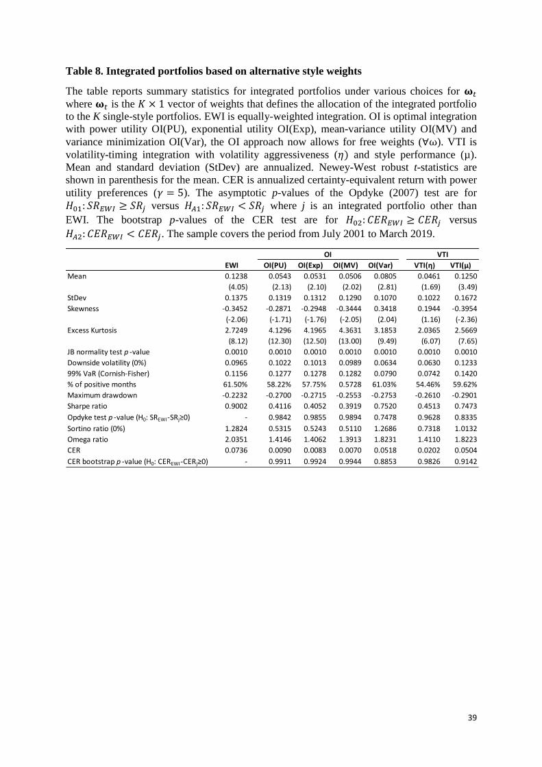
39
Table 8. Integrated portfolios based on alternative style weights
The table reports summary statistics for integrated portfolios under various choices for
where is the vector of weights that defines the allocation of the integrated portfolio
to the K single-style portfolios. EWI is equally-weighted integration. OI is optimal integration
with power utility OI(PU), exponential utility OI(Exp), mean-variance utility OI(MV) and
variance minimization OI(Var), the OI approach now allows for free weights ( ). VTI is
volatility-timing integration with volatility aggressiveness ( and style performance (µ).
Mean and standard deviation (StDev) are annualized. Newey-West robust t-statistics are
shown in parenthesis for the mean. CER is annualized certainty-equivalent return with power
utility preferences ( ). The asymptotic p-values of the Opdyke (2007) test are for
versus where j is an integrated portfolio other than
EWI. The bootstrap p-values of the CER test are for versus
. The sample covers the period from July 2001 to March 2019.
EWI OI(PU) OI(Exp) OI(MV) OI(Var) VTI(η) VTI(μ)
Mean 0.1238 0.0543 0.0531 0.0506 0.0805 0.0461 0.1250
(4.05) (2.13) (2.10) (2.02) (2.81) (1.69) (3.49)
StDev 0.1375 0.1319 0.1312 0.1290 0.1070 0.1022 0.1672
Skewness -0.3452 -0.2871 -0.2948 -0.3444 0.3418 0.1944 -0.3954
(-2.06) (-1.71) (-1.76) (-2.05) (2.04) (1.16) (-2.36)
Excess Kurtosis 2.7249 4.1296 4.1965 4.3631 3.1853 2.0365 2.5669
(8.12) (12.30) (12.50) (13.00) (9.49) (6.07) (7.65)
JB normality test p -value 0.0010 0.0010 0.0010 0.0010 0.0010 0.0010 0.0010
Downside volatility (0%) 0.0965 0.1022 0.1013 0.0989 0.0634 0.0630 0.1233
99% VaR (Cornish-Fisher) 0.1156 0.1277 0.1278 0.1282 0.0790 0.0742 0.1420
% of positive months 61.50% 58.22% 57.75% 0.5728 61.03% 54.46% 59.62%
Maximum drawdown -0.2232 -0.2700 -0.2715 -0.2553 -0.2753 -0.2610 -0.2901
Sharpe ratio 0.9002 0.4116 0.4052 0.3919 0.7520 0.4513 0.7473
Opdyke test p -value (H0: SREWI-SRj≥0) - 0.9842 0.9855 0.9894 0.7478 0.9628 0.8335
Sortino ratio (0%) 1.2824 0.5315 0.5243 0.5110 1.2686 0.7318 1.0132
Omega ratio 2.0351 1.4146 1.4062 1.3913 1.8231 1.4110 1.8223
CER 0.0736 0.0090 0.0083 0.0070 0.0518 0.0202 0.0504
CER bootstrap p -value (H0: CEREWI-CERj≥0) - 0.9911 0.9924 0.9944 0.8853 0.9826 0.9142
VTIOI

40
Table 9. Economic sub-period analysis
The table reports the annualized Sharpe ratio of the long-only baseline AVG portfolio (Panel
A) and of each long-short portfolio (Panels B and C) over various sub-periods: high versus
low volatility regimes, pre- versus post-financialization (dated on January 2006), NBER-
dated recession and expansion periods, and the 2008 oil price bubble-bust period (July 2008 –
February 2009) versus the remaining of the sample (Other). TS is term structure, HP is
hedging pressure, SP is speculative pressure, Mom is momentum, EWI is equally-weighted
integration, OI is optimal integration with power utility (PU), exponential utility (Exp),
mean-variance utility (MV) and variance minimization (Var), VTI is volatility-timing
integration.
July 2008 -
Feb 2009Other
Panel A: Long-only portfolio
AVG -0.5236 0.2819 0.5694 -0.3701 0.1027 -1.0256 -5.9675 0.1610
Panel A: Single-style portfolios
TS 0.7350 0.5732 0.0076 0.8710 0.8224 -0.5176 0.7892 0.6323
HP 0.4539 0.6593 0.3434 0.6276 0.5539 0.6933 0.4029 0.6038
SP 0.6722 0.6518 0.2583 0.8316 0.6437 0.7372 1.0957 0.6231
Mom 0.8236 0.7026 0.9293 0.6983 0.8357 0.1083 1.8862 0.7072
Value 0.4070 0.2536 1.4370 -0.0846 0.2856 0.4934 0.3188 0.3167
Liquidity -0.0742 0.2416 -0.2752 0.2448 0.1499 -0.1063 2.4255 0.0251
Skewness 0.0558 -0.0722 -0.1763 0.0517 0.1203 -0.9541 0.1815 -0.0245
Panel B: Integrated portfolios
EWI 0.9117 0.8896 0.7553 0.9466 0.9960 0.1984 2.9989 0.8284
OI(PU) 0.9268 0.7654 1.2635 0.6995 0.8813 0.4576 1.6951 0.7800
OI(Exp) 0.9242 0.7473 1.2614 0.6861 0.8677 0.4625 1.7282 0.7683
OI(MV) 0.9081 0.6247 1.2553 0.5967 0.7788 0.4638 1.8158 0.6915
OI(Var) 1.0286 0.6266 0.8032 0.7545 0.7818 0.5825 3.3409 0.6753
VTI 0.7390 0.8478 0.4862 0.9106 0.8767 0.3349 2.2179 0.7404
Expansion
Expansion versus
recession
High versus low energy
volatility
Low Post
Pre and post
financialization
High Pre Recession
M
e
a
n
r
Bust of 2008 oil price
bubble

41
Figure 1. Future value of $1 invested in long-only and long-short single-style energy
portfolios
TS is term structure, HP is hedging pressure, SP is speculative pressure, Mom is momentum.

42
Figure 2. Future value of $1 invested in long-short integrated portfolios
EWI is equally-weighted integration, OI is optimal integration with power utility (PU),
exponential utility (Exp), mean-variance utility (MV) and variance minimization (Var), VTI
is volatility timing integration.


