
R73-12
pen n _ 1 ~. 5 ;J 11.S
Soils Publication No. 317
Optimum Seismic Protection
and
Building Damage Statistics
Report No.6
THE SHEAR WAVEVELOCITY OF
BOSTON BLUE CLAY
by
Paul Joseph Trudeau
Supervised by
Robert V. Whitman
John T. Christian
February, 1973
Sponsored by National Science Foundation
Grants GK-279SS and GI-29936
EASINFORMAcTION RESOURCESNATIONAL SCIENCE FOUNDATION

c
OPTIMUM SEISMIC PROTECTION AND
BUILDING DAMAGE STATISTICS
Sponsored by National Science Foundation
Grants GK- 27955 and GI- 2 9936
Report No. 6
THE SHEAR WAVE VELOCITY
OF
BOSTON BLUE CLAY
by
PAUL JOSEPH TRUDFAU
Supervis ed by
Robert V. Whitman
John T. Christian
February, 1973
R 73- 12 Soils Publication No. 317


ABSTRACT
The purpose of this report is to provide a best estimate of the
shear wave velocity of Boston Blue Clay to be used in soil amplification
studies in the design of structures in the Boston area against earth
quakes. The in situ shear wave velocities determined using the cross
hole method by Weston Geophysical Research, Inc. are compared
with values obtained using MIT's Hardin Oscillator and also empirical
correlations proposed by Hardin and Black. Modifications to the
laboratory values and the empirical results indicated herein agree
favorably with the in situ shear wave velocities of 850 to 900 feet
per second.
1

PREFACE
This is the sixth report prepared under National Science Foundation
grants GK-27955 and GI-29936. This report is identical with a
thesis written by Paul J. Trudeau in partial fulfillment of the require
ments for the degree Master of Science. The research was supervised
by Robert V. Whitman and John T. Christian, profes sor s of Civil
Engineering. Acknowledgement and thanks are due to Mr. Charles
Guild of the American Drilling and Boring Company who generously
contributed the borings, to Mr. Vincent Murphy of Weston Geophysical
Research, Inc. who generously contributed the in situ wave velocity
measurements, and to Prof. Kenneth H. Stokoe of the University of
Massachusetts who gave valuable advice concerning the conduct of
the resonant column tests.
A list of previous reports appears on the next sheet.
2

LIST OF PREVIOUS REPORTS
1. Whitman, R. V., Cornell, C. A., Vanmarcke, E. R., and Reed,J. W.: "Methodology and Initial Damage Statistics, II Departmentof Civil Engineering Research Report R72-l7, M.1. T .• March, 1972.
2. Leslie, S. K., and Biggs, J. M .• "Earthquake Code Evolutionand the Effect of Seismic Design on the Cost of Buildings, "Department of Civil Engineering Research Report R 72-20,M.1. T., May, 1972.
3. Anagnostopoulos, S. A., IINon-Linear Dynamic Response andDuctility Requirements 0 f Building Structures Subjected toEarthquakes. II Department of Civil Engineering ResearchReport R72-54, M.1. T., September, 1972.
4. Biggs, J. M., and Grace, P. R., IISeismic Response of BuildingsDesigned by Code for Different Earthquake Intensities," Department of Civil Engineering Research Report R 73-7, January, 1973.
5. Czarnecki, R. M., 'IEarthquake Damage to Tall Buildings, IIDepartment of Civil Engineering Research Report R 73 - 8,M.1. T., January, 1973.
3

TABLE OF CONTENTS
ABSTRACT
PREFACE
LIST OF PREVIOUS REPOR TS
LIST OF FIGURES
CHAPTER I INTRODUCTION
CHAPTER II IN SITU SHEAR WAVE VELOCIES
CHAPTER III LABORATORY TEST PROGRAM
3.1 Introduction
3. 2 Determinahon of Index Properties
3.3 Apparatus and Procedure for Hardin Oscillator
Calibration Factors
3.4 Tests on Boston Blue Clay
Procedure for Controlling Strain
Chamber Fluid
Mercury as Chamber Fluid
3. 5 Conclusion
CHAPTER IV ESTIMATES OF SHEAR WAVE VELOCITY
4.1 Introduction
4. 2 In Situ Results
4. 3 Laboratory Results
CHAPTER V SUMMARY AND CONCLUSIONS
4
1
2
3
6
7
12
14
14
15
Test 15
17
18
18
19
20
22
23
23
23
23
27

TABLE OF CONTENTS (Continued)
TABLE 4.1
FIGURES
APPENDIX A
APPENDIX B
LIST OF REFERENCES
5
29
30
45
55
61

LIST OF FIGURES
1. 1 A Typical Profile for the Boston Basin Area 30
1. 2 General Location of Profiles in the Bo ston Ba sin Area 31
1. 3 Bo ston Quake Boring Locahons 32
1. 4 Bo ston Quake Profile 33
3.1 K vs. PI (in Hardin-Black Equation) 34
3.2 Index Properties vs. Depth 35
3. 3 Driving Unit of Hardin Oscillator 36
3.4 Hardin Oscillator Set- Up in Triaxial Cell 37
4.1 TESTS T-3 and T-4 38
4.2 TEST C-l 39
4.3 TEST L-l 40
4.4 TESTS S-l and S-2 41
4.5 TEST G-l 42
4.6 TEST AA-l 43
4.7
A-l
A-2
A-3
Shear Wave Velocity vs. Depth
C and A vs. Periods T
C vs. Log TiITle for Test G-ls
SysteITl Factor vs. F
6
44
51
53
54

CHAPTER I
INTRODUCTION
The objective of this study is to provide a best estimate of the
shear wave velocity of Boston Blue Clay (BBC) to be used in soil amplif-
ication studies (Seed and Idriss, 1969) in the design of structures in the
Boston area against earthquakes. The significance of the shear wave
velocity to the analysis of small amplitude soil vibration problems has
been discussed by Hardin and Black (1968) and the application of this
parameter to the design and analysis of foundation vibrations has been
presented by Whitman and Richart (1967). Presented herein will be the
work leading up to and including the determination of the shear wave
velocity of Boston Blue Clay.
This clay was transported by preglacial streams and deposited
m the quiet marine waters of the Boston Basin during the Boston sub-
stage of the Wisconsin Glacier (approximately 20, 000 years ago.
Chute, 1959). To indicate the extent of the clay layer an investigation
was undertaken. This soil survey was initiated by collecting and
analyzing the extensive data that is available for the Massachusetts
Institute of Technology (MIT) campus. Another source was the numer-
ou s projects that MIT personnel have been involved with: for example,
Interstate 95 in Saugus, Green Shoe Factory in the South Boston area,
and the University of Massachusetts site at Columbia Point. This
starting point gave a good picture of the types of profiles which are to7

be expected in the Boston Basin area. A later interview with Clifford
Kaye of the United States Geological Survey (USGS) in Boston generally
confirmed these data,
The profiles are somewhat similar and are differentiated mainly
by the thicknes s of the clay layer. They are, in general, starting from
bedrock (which is the Cambridge Argillite in the Basin area) and working
up: bedrock, glacial till, outwash sands and gravels, clay (less than
60 feet to a maximum of about 180 feet), outwash sands and gravels,
peat and/or organic silt, and heterogeneous man-placed fills. This
general scheme is shown in Figure 1. 1.
Discussion with other members of the Ge"otechnical Division at
MIT yielded five typical profiles of which three were clay profiles of
the type in Figure 1. 1 with only the thicknes s of clay varying:
Ca se 3 - Up to 60 feet of clay
Case 4 - 60 to 120 feet of clay
Case 5 - 120 to 180 feet of clay.
Case 1 was to be up to 30 feet of fill or silt on firm soil (i. e. till) or
rock and Case 2 was Case 1 located above 10 to 30 feet of outwash sands
and gravels on rock.
These profiles were then located on a USGS Boston and Vicinity
topographic map, Additional subsurface data was obtained from the
1961 Boston Society of Civil Engineers' collection of boring data in the
Boston area. This map, shown in Figure 1. 2, not only located these
8
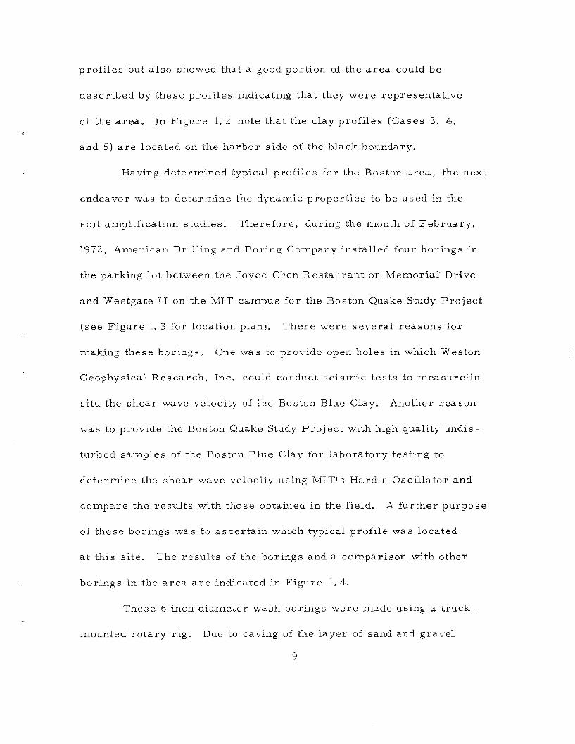
profiles but also showed that a good portion of the area could be
described by these profiles indicating that they were representative
of the area. In Figure 1. 2 note that the clay profiles (Cases 3, 4,
and 5) are located on the harbor side of the black boundary.
Having determined typical profiles for the Boston area, the next
endeavor was to determine the dynamic properties to be used in the
soil amplification studies. Therefore, during the month of February,
1972, American Drilling and Boring Company installed four borings in
the parking lot between the Joyce Chen Restaurant on Memorial Drive
and Westgate II on the MIT campus for the Boston Quake Study Project
(see Figure 1. 3 for location plan). There were several reasons for
making these borings. One was to provide open holes in which Weston
Geophysical Research, Inc. could conduct seismic tests to measure in
situ the shear wave velocity of the Boston Blue Clay. Another reason
was to provide the Boston Quake Study Project with high quality undis
turbed samples of the Boston Blue Clay for laboratory testing to
determine the shear wave velocity using MIT's Hardin Oscillator and
compare the results with those obtained in the field. A further purpose
of these borings was to ascertain which typical profile was located
at this site. The results of the borings and a comparison with other
borings in the area are indicated in Figure 1. 4.
These 6 inch diameter wash borings were made using a truck
mounted rotary rig. Due to caving of the layer of sand and gravel
9

between the depths of 15 and 45 feet, 6 inch diameter steel casing was
installed for the first 50 feet of these holes. The holes were extended
through the clay and clayey sand from 50 feet to 175 feet using drilling
mud to keep them open. At a depth of 17 5 feet a very dens e (120 blows /
4 inches) fine sand layer was encountered and the holes were discon
tinued. At the completion of each hole, 4 inch O. D. plastic (PVC)
pipe in 20 foot lengths connected with 4- 3/4 inch O. D. couplings was
installed in the holes. This plastic casing was lowered open-ended
inside the 6 inch steel casing. At a depth of about 100 feet this casing
required pushing - - - first by hand, and then the la st two sections with
the use of the hydraulic jack on the truck-1TIounted rotary rig. After
the plastic casing was installed, the drillers then lowered A- rods with
which they wa shed out the material that had collected inside the pIa stic
casing. The 6 inch steel casing was then removed using the conventional
"bumping out" procedure.
In Hole B-1, undisturbed samples (3 inch Shelby tubes) were
taken continuously through the clay layer (from a depth of about 50 feet
to about 110 feet). These samples were taken with a fixed piston type
sampler. Laboratory testing was performed on these samples to
obtain values of the shear wave velocity and also to obtain the para
meters necessary for use in empirical relationships.
This thesis presents the results of the Hardin Oscillator tests
10

on these undisturbed saInples. The shear wave velocities deterInined
by Weston Geophysical Research, Inc. in situ are compared with these
results and also with the results of eInpirical correlations using soil
paraIneters obtained froIn the laboratory testing of the undisturbed
saInples. Finally, a conclusion regarding the best estiInate of the
shear wave velocity of Boston Blue Clay is drawn.
11

CHAPTER II
IN SITU SHEAR WAVE VELOCITIES
Thein situ shear wave velocities were detenuined by Weston
Geophysical Research, Inc e in May, 1972 at the site on the MIT campus.
The testing program, utilizing the four boreholes which were described
in Chapter I, consisted of the cross-hole method. For a detailed
description of this method of seismic testing see Stokoe (1972).
Basically, the cros s -hole method mea sure s the time it takes for a
shear wave to travel a known distance. The shear waves are generated
at a certain depth in one borehole while sensors at the same level in
the other borehole( s) await their arrivaL Knowing the time it takes
for the shear waves to travel through the soil and the distance between
the boreholes, one can compute the shear wave velocity of the soiL
In this testing program blasting caps (lor sometimes 2) were
detonatedm one of the boreholes as the source of the shear waves.
The sensors consisted of three velocity transducers, one horizontal,
and the other two vertical, which were lowered to the same depth in
the other three boreholes. Nothing was done to insure that the jugs
containing the velocity transducer s were well- coupled to the soil, for
it was assumed that they would rest against the inside of the casing.
The testing was begun at the bottom of the casing and then measure-
ments were taken at ten foot intervals coming up the profile. The
testing was done in this manner because the blasting caps destroyed12

the plastic pipe thus preventing the lowering of subsequent charges to
greater depthso For this reason, Weston took many readings at the
sarne elevation before moving up the hole, to insure acceptable results,
The location plan of these borings is shown in Figure 1. 3 0 The
results of the in situ shear wave velocity determinations are shown
in Chapter IV. Figure 4. 7 indicates that the value of the shear wave
velocity of the Boston Blue Clay as obtained in the field is approximately
850 feet per second.
13
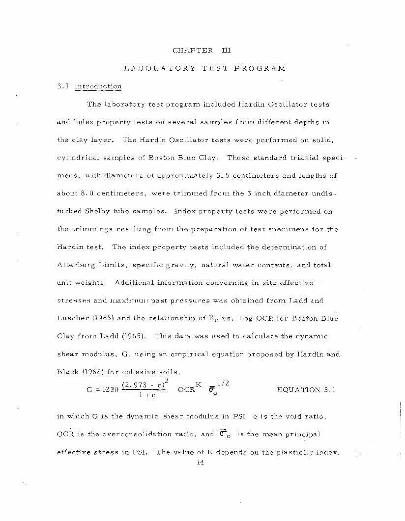
CH.APTER III
LABORATORY TEST PROGRAM
3. 1 Introduction
The laboratory test program included Hardin Oscillator tests
and index property tests on several samples from different depths in
the clay layer. The Hardin Oscillator tests were performed on solid,
cylindrical samples of Boston Blue Clay. The se standard triaxial speci-
mens, with diameters of approximately 3.5 centimeters and lengths of
about 8,0 centimeters, were trimmed from the 3 inch diameter undis-
turbed Shelby tube samples. Index property tests were performed on
the trimmings resulting from the preparation of test specimens for the
Hardin test. The index property tests inchl,ded the determination of
Atterberg Limits, specific gravity, natural water contents, and total
unit weights. Additional information concerning in situ effective
stresses and maximum past pressures was obtained from Ladd and
Luscher (1965) and the relationship of K o vs. Log OCR for Boston Blue
Clay from Ladd (1965), This data was used to calculate the dynamic
shear rnodulus, G, using an empirical equation proposed by Hardin and
EQUATION 3.11/2
~K
OCR
(1968) for cohesive soils,2
G = 1230(2.97~ - e)l+e
Black
in which G is the dynamic shear modulus in PSI, e is the void ratio,
OCR is the overconsolidation ratio, and ero is the mean principal
effective stress in PSI. The value of K depends on the plastici.~/ index,
14

PI, of the soil as shown In Figure 3.1.
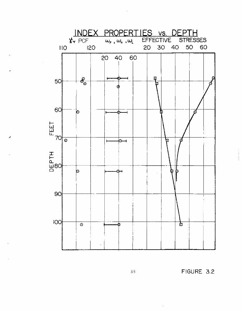
3. Z Determh~.ation of Index Properties
The index property tests were performed according to the
procedures in Lambe (1951), except for the total unit weights, which
were determined by measuring and weighing the Hardin test specimens
immediately after trimming. The results of the Atterberg Limits
indicated a PI of about 30 leading to K=Oc 24. Calculations indicated
that the in situ void ratio was approximately equal to 1. 0 which is
typical for Boston Blue Clay. Using the appropriate parameters in
Equa tion 3. 1, value s of G wer e obtained for each test specimen. The
shear wave velocity was then calculated using
EQUATION 3. Z
in which C s is the shear wave velocity, G is the shear modulus, and p
1S the mass density which equals t WT' the total unit weight divided
by g, the acceleration of gravity. These results are shown in
Figure 4. 7 and the results of the index property tests are shown in
Figure 3. Z.
3.3 Apparatus and Procedure for the H?-E..:J::.in .9scillator Test
The Hardin Oscillator test is used to determine the dynamic
shear modulus of a sample by the resonant column method. The reso-
nant column method is described by Richart, Hall, and Woods (1970)
15

and Hardin and Mos sbarger (1966). The Hardin Oscillator test - -
apparatus, procedure, and theory - - - is described by Hardin and
Music (1965) and also by Hardin (1970).
The Hardin apparatus applies a torsional vibration to one end
of a specimen within a triaxial celL A load cell is included within the
apparatus (see Figure 3.3) so that anisotropic states of stress similar
to estimated in situ stresses can be applied to the specimen within the
triaxial cell during the dynamic test. Figure 3.4 shows the apparatus
in position for testing. Figure 3. 3 shows the oscillator portion of the
Hardin device. The electromagnets in Figure 3. 3 are excited by an
AC current from the audio oscillator (Hewlett Packard Model 200-AB)
producing a sinusoidally varying torque at the top of the specimen.
The base of the specimen rests upon a rigid pedestal which has suffi
cient inertia to rnake the motion of the attached end of the specimen
essentially zero during vibration of the specimen (Hardin, 1970).
An accelerometer (see Figure 3.3) is attached to the oscillator to
monitor the movement of the top of the specimen. The frequency of
oscillation is varied until the maximum output of the accelerometer
i.s obtained. This output is monitored with an oscilloscope or can be
measured with an AC voltmeter. The resonant frequency of the system
and specimen occurs when the maximum output of the accelerometer is
achieved. Knowing the calibration of the accelerometer, the test can
be run at a certain level of shear strain by varying the input voltage
16

and the frequency such that the desired output of the acceleroITleter is
obtained. The theory presented by Hardin and Music (1965) or Hardin
(1970) uses this resonant frequency to deterITline the dynaITlic shear
ITlodulus. Equation 3.2 is then used to obtain the shear wave velocity.
Calibration Factors: During the course of the testing prograITl
there was SOITle question as to what were the appropriate calibration
factors. It was found that these factors, as discussed in Hardin (1970)
or Hardin and Music (1965), changed with different strain levels for the
MIT Hardin Oscillator. These changes led to iITlproper trends in the
results, i. e. C s was greater for higher shea:r strains, which is not
true (Hardin and Black, 1968). Telephone conversations with Dr.
Hardin at the University of Kentucky and with Dr. Stokoe at the Univer-
sity of Massachusetts at AITlherst both proved fruitless, for this
phenoITlenon did not exist with the equiprr.ent they had used. It was
concluded that the calibration factors corresponding to low strain aITlp-
litudes be used and thus, only the low strain aITlplitude data froITl these
tests is included in this report. Note that Hardin (1970) recoITlITlends
-5using an average shear strain of about 2.5 x 10 in/in and the shear
~
strains in these tests are close to this value (see Table 4.1).
3.4 Tests on Boston Blue Clay
Procedure for Controlling Strain: There were two different
procedures used for these tests. The earlier tests were run at three
17

different levels of input voltage of the Hewlett Packard audio oscillator
corresponding to a maxiInum shear strain, at any point of the specimen,
of about 2.5, 5, and 10 x 10- 5 in/in. This strain refers to the maximum
movement at the circumference of the solid sample. For solid samples
Hardin and Drnevich (1972) define average shear strain as equal to
I area (strain) dA / AREA which leads to an average shear strain equal
to 2/3 of the maximum. shear strain. The later tests were run at a
maximum shear strain of approximately 1 x 10 -5 in/in (An illustration
of how the shear strain is controlled during the test is shown on page
of Appendix A.) in an attempt to obtain the maximum value of the
dynamic shear modulus. Note that the dynamic shear modulus decreases
with increasing strain and 1 x 10⁻⁵
in/in is the lowest strain at which
satisfactory measurements can be made due to random AC noise in the
cathode follower used to couple the output of the accelerometer to the
measuring devices.
The initial tests included T-3, T-4, S-l, and S-2. (See Appendix
B for a general description of each test.) These tests were isotropi
cally consolidated to the estimated in situ horizontal effective stress,
at which point the resonant frequency was determined. Subsequently,
the cell pressure was increased to the estimated in situ vertical
effective stress, again the specimen was consolidated, and the dynamic
test run. The specimens were then consolidated to higher cell pressures
in approximately 20 PSI increments, up to a maximum cell pressure
18

of 100 PSI. After running the dynamic test at the maximum confining
pressure, the samples were unloaded in 20 - 40 PSI steps, allowed
time to rebound, and then the dynamic tests were run again.
Chamber Fluid: A major problem results due to the electrical
connections within the triaxial cell. The connections must not be
submerged in a fluid that conducts electricity; therefore, the cell
can only be filled with a cell fluid up to the base of the oscillator. The
cell pressure is then applied by air pres sure acting on the fluid within
the cell. The use of water or silicone oil as a cell fluid does not provide
adequate protection from the diffusion of air, especially under pressures
greater than 30 PSI, through the cell fluid and the membrane where, at
atmospheric pressure, it comes out of solution thus interfering with
volume change readings. An attempt was made to use silicone oil as a
cell fluid completely filling the cell and using mercury pots to apply
the cell pressure. However, the 5 centistoke silicone oil was too
viscous and it was thought that the movement of the magnets induced
motion in a certain mass of the oil thus interfering with the resonant
frequency of the sample. Therefore, the tests were run with silicone
oil only covering the sample and air pressure was applied to the top
of the cell. (Silicone oil was used instead of water because water
a ttacks the air pistons and aluminum of the support device for the
Hardin apparatus during the set-up of the test.) Volume change readings
were not made after the results of the first few tests indicated that they
19

were no good. During subsequent tests an attempt was made to keep
the sample wet by flushing water through the porous stone at the base
of the specimeno It was found that consistent results of the resonant
frequency could be obtained by this procedure as long as the filter
strips surrounding the specimen were kept wet. It was found that
flushing water through the porous stone once a day was sufficient to
remove the air bubbles and to keep the filter strips wet. Consolidation
was obtained by allowing approximately 24 hours to pass before running
the dynamic test. From past testing on Boston Blue Clay (Edgers, 1967)
this was considered more than adequate time for primary consolidation.
Mercury as Chamber Fluid: At the time of this writing,
Marcuson and Wahls (1972) have published results of a series of tests
on two different clays. They used a Hardin Oscillator, performing
tests in essentially the same manner as the earlier tests described
above, i. e. they ran the dynamic tests a t thre~ different strain levels
and different cell pres sures up to 100 PSI. However, they us ed
mercury a s the cell fluid surrounding the sample because air does not
diffuse readily into mercury at the cell pres Bures involved. They
ran tests on the same sample surrounded by mercury and then with the
mercury drained out. They found little variation in G (about 7 % at
10 PSI with Q=0.0006 radians) and no definite trend as the cell pres-
sure was increased. Thus, they conclude that the use of mercury is
an effective means of elimina Eng the problem of air diffusion during20

long term tests. However, they caution that the mercury results in a
pressure differential of about 1. 5 PSI from the top to the bottom of
the specimen and therefore, may have a significant effect at low con-
fining pressures. Surrounding the sample with mercury allows volume
changes to be measured with a burette. Furthermore, a backpressure
can be used to maintain a completely saturated specimen.
The later tests, C-l, C-2, G-l, L-l, and AA-l, were run at a
maximum shear strain of about 1 x 10 -5 in/in. These tests were
loaded isotropically to the in situ effective octahedral stress as com-
puted using the values of vertical effective stress and maximum past
pressure as shown in Figure 3.2, and the values of K o as determined
by Ladd (1965) for Boston Blue Clay. The dynamic test was run at a
maximum shear strain of 1 x 10 -5 in/in obtaining values of the reso-
nant frequency with time in a manner similar to a consolidation test.
The value of the shear wave velocity, C s ' was then plotted vs. the
logarithm of time as shown in Figures 4.5 and 4.6. To compare these
results with the initial tests, Tests C-l and L-l were then loaded
isotropically to higher cell pressures, and again C s was determined
vs. the logarithm of time, Running the test in this manner allowed
observation of the results while the specimen was consolidating under
each increment of load. Note in Figures 4.5 and 4.6 that after
primary consolidation had been completed there was an increase In C s
vs. time. This increase is linear on the C s vs. Log time plot and21

has been noted in tests on cohesive soils by Stokoe (1972) and Hardin
and Black (1968). This increase equalled approximately 40 feet per
second per log cycle of time and was used to extrapolate the laboratory
values of C s to those expected in the field as will be shown in
Chapter IV.
3. 5 Conclu sion
Reported herein are the results of the index property tests.
Also included is the description of the Hardin Oscillator test --- appa
ratus, procedure, and the problerns encountered during this study.
Important variables during the performance of the Hardin test include
the level of the shear strain, consolidation and drainage of the specimen
during long term tests, effects of chamber fluid, and the effects of
time on the results. Using water (or silicone oil) as the cell fluid upon
which air pressure was applied resulted in problems due to air diffusion
into the specimen. If this air was removed by flushing water through the
porous stone daily, no change in the measured shear wave velocity
occurred. Thus it is concluded that if water is to be used as the cell
fluid, adequate provisions must be made to insure that the specimen IS
kept weL
22

CHAPTER IV
ESTIMATES OF SHEAR WAVE VELOCITY
4.1 Introduction
The results of this investigation are presented in this chapter.
These results include the in situ shear wave velocities measured by
Weston Geophysical Research, Inc., the Hardin Oscillator test results,
and the results from Hardin and Black's empirical correlation (Eq. 3.1)
for cohesive soils. Also included are the corrections to the laboratory
results based on strain levels and secondary time effects.
4. 2 In Situ Results
The in situ results by Weston Geophysical Research, Inc. are
presented in Table 4.1 and are also plotted in Figure 4.7. Weston
reported that some of their records were good and some were poor.
The majority of the records were average, or at least acceptable.
There was some problem due to coupling of the output velocity trans-
ducers to the ground due to a possible gap between the plastic casing
and the soil. However, a s will be shown later, thes e results agree
well with the laboratory results. Weston reports that these values of
C s are good to within 10%.
4. 3 Laboratory Re sults
The results of the laboratory tests that were run at different
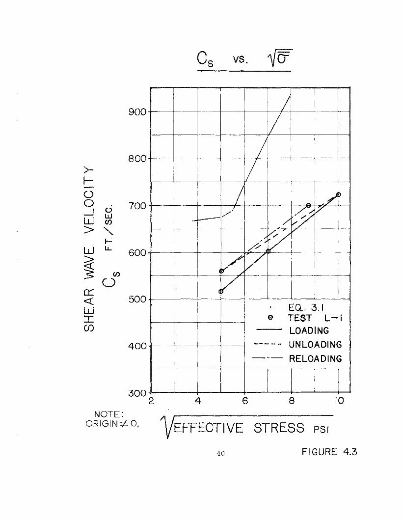
confining pressures are presented as plots of the shear wave velocity23
vs. the square root of the effective isotropic confining pressure in
Figure 4. 1 to 4.4. The shear wave velocities that are plotted are
the values of C s that were mea sured and corrected for strain amp-
Etude. Also shown on these plots are the values of C s as predicted
by Hardin-Black (Equation 3.1). The values of C s at the effective
In situ octahedral stresses were then interpolated from these results
to obtain the values of C s in column 4 on Table 4.1. Tests G-l and
AA-l were only run at the in situ effective octahedral stress and,
therefore, the results are presented as plots of C s vs. Log time In
Figures 4. 5 and 4.6. The reader is cautioned that due to problems
during the running of thes e tests some of the results are suspect.
These problems, mainly due to air diffusion into the specimen, are
inumera ted in Appendix B.
Table 4.1 is a summary of the results of this study for the
specimens at the in situ effective octahedral stresses. The values of
C s (column 1) is the value of the shear wave velocity measuredmeas
using the Hardin Oscillator at an elapsed tirne of approximately 1000
minutes and a cell pressure equal to the estimated in situ effective
octahedral stresses. These values were obtained at the maximum
shear strains indicated in column 2. In order to compare results for
the same strains, the C s are divided by column 3, the equivalentmeas
Cs/Csmax. The values of equivalent Cs/Csmax equal the square
root of the values given by Hardin and Drnevich (1972) for G/Gmax '
24

Note that there is little difference in C s (column 4) and Cmax smeas
(column 1) using the Hardin apparatus. The computed values of C s
using the Hardin-Black equation (Eq. 3.1) are indicated in column 5.
These results are greater than the measured values by more than
200 feet per second, but recall that the measured values of C s were
at an elapsed time of 1000 minutes. Plots of C s vs. Log time, as
In Figures 4.5 and 4.6, show that there exists a linear increase in
C s vs. Log time during secondary consolidation. This increase has
been noted by others for cohesive soils (Hardin and Black, 1968;
Stokoe, 1972; and Marcuson and Wahls, 1972), and in these tests was
approximately 40 feet per second per log cycle. Considering this
increase to continue for a length of time equal to the age of the clay
(about 20,000 years) yields the values of C s20 ,000 in column 7.
These values are surprisingly close to the results obtained in situ by
Weston Geophysical Re.search, Inc.
Hardin and Black (1968) analysed this effect and also the effect
of different load increments. They conclude that there is a secondary
increase of the vibration shear modulus with time at a constant effective
stress that is not accounted for by changes in void ratio. Furthermore,
this increase can be destroyed by changes in effective stress and
consequently, this effect may be quite important with soils in situ, for
the laboratory values of shear modulus (shear wave velocity) depend
on the loading scheme used. Tests which Hardin and Black ran on a
25

Kaolin clay using small load increments (about 1 PSI) yielded values
of shear modulus which were about 20% greater than those predicted
by their equation. These data fit the equation
G= 1630(2.973 _ e)2
1 + e
- 1/200 EQUATION 4.1
more closely. Using Equation 4.1 together with the parameters for
the specimens of Boston Blue Clay tested yields the values in column 8
of Table 4.1. Note that these values are in better agreement with the
laboratory values which were extrapolated to 20, 000 years and also the
in situ values by Weston Geophysical Research, Inc. than those calcu-
la ted using EquaHon 3.1. This agreement is more easily seen In
Figure 4.7 which is a plot of the data in Table 4.1.
Insofar as the laboratory test results and the calculated results
using Equation 4.1 agree reasonably with the in situ results, the author
concludes that the in situ results are probably the best estimate of the
shear wave velocity of Boston Blue Clay. Figure 4.7 indicates that
C s varies between 850 and 900 feet per second depending on the depth.
This value corresponds to a shear modulus of approximately 19, 000 PSI
for the Boston Blue Clay.
26

CHAPTER V
SUMMARY AND CONCLUSIONS
Based on the results of this study, it is the conclusion of the
author that the best estimate of the dynamic shear wave velocity of
Boston Blue Clay is between 850 and 900 feet per second. This
range is substantiated by the in situ measurements made by Weston
Geophysical Research, Inc. utilizing a seismic technique known as the
cross-hole method. Close agreement with these values is found by
extrapolating the laboratory values of the shear wave velocity meas
ured using MIT's Hardin Oscillator to a time equivalent to the age of
the clay. The laboratory values were found to increase linearly with
the logarithm of time during secondary consolidation as was the case
with numerous researchers (Hardin and Black, 1968; Stokoe, 1972;
Marcuson and Wahls, 1972). This linear trend in the shear wave vel
ocity vs. the logarithm of time, coupled with the close agreement of
the extrapolated results to the in situ results, was considered justifi
cation for the extrapolation of the laboratory data. Utilizing parameters
of the samples of Boston Blue Clay tested, an empirical correlation,
when modified according to results presented by Hardin and Black
(1968) to account for the increase in dynamic modulus with time during
secondary consolidation and the effects of small load increments, also
yielded values of shear wave velocity close to this range. Therefore,
27

based on in situ results and modified laboratory and empirical results,
it is concluded that the best estimate of the shear wave velocity of
Boston Blue Clay is 850 to 900 feet per second.
28

TABLE 4.1
SHEAR WAVE VELOCITY DATA FOR SSG
2 3 4 5 6 7 8 9
N--D
: C 't'ei. """'.t.E.QUIV. C~ CS -.", C !S"E.CON PAav Cs Cs CSTEST S I'\IA.~. c~ ter \6(,~
S TIMEA"r 10 m "AA-l&l~ E I' rIC'" S 1.0 000 ~... _FIEll ~ILI ..>it; 'J.TO N
-5 F?SFPS -.<.10 ~ FPS FPS FPS FPS FPSIN Lo~ C~c....E. t
T-3~4 535 2.5-5 0..99 540 772 40~}~45 1022 840-- ----- ----
C-I~2 564 i 0.99 570 747 41 I 984 990 840
G-I 490 I 0.99 496 701 44 i 940 930 850 II
-- ------ .- ... -------------.- --- ---- C T-- r-----· .--L-I 510 I 0.99 515 675 39 910 895 875
--.-----.-- - ---_·_-_·-----1- -. - -- ----....---
8'-2 480 1-10 0.91 495 732 40"* I 908 970 900
I 8-1 u 436 5 -7 O.9~_~445_c 732__ ~O* ~!55 97~_, 900
AA-I 508 I 0.99 513 717 44 I 958 951 850
"* ASSUMED

MAN~PLACED FILLS
PEAT AND/OR ORGANIC. SILT
OUTWASH SANDS AND GRAVELS
CLAY
OUTWASH SANDS AND GRAVELS
GLACIAL TILL
BEDROCK~CAMBRIDGE ARGILLITE
A TYPICAL PROFILE FORBOSTON BASIN AREA
30 FIGURE 1.1

GENERAL LOCATION OF PROF ILESIN THE BOSTON BAS IN AREA
FIGURE 1.2

TO WESTGATE II J
FIGURE 1.3
wozWLL
I
en8-2 --L
n
...0'>0'>0'>
nnnD
-""..
~-.J "".
« ,0:::0:2:lJJ
T~ 8-4....0l()C\J
IC\J0C\JI
CD
t32
w>0:::o

BOSTON QUAKE PROFILE
8-202
rv350'-----......~I
8-1
v,V
to • •
DEPTH0'
• +++ FILLV/h ORGANIC MAT'L.
q.; SAND AND,~'.' GRAVEL'V."
8-103
~ I'V 200 I ---+-I~~r-----
BOSTON
BLUE
CLAY
50'
,. :-:" .
.. ,.. ",
.. ' '."
I '"
. .~ • t..• • II
: \ ',',
f· .. ,
I' ••, • I
" .~
:. " f:
. -" • "
0; •
. . ~.,
" ........
SAND
STRATIFIED
WITH
CLAY
100'
· ". :· ....'., .' .
150'.. ....
· .~ .•• : I I,
': .. , SAND I ... a
B-103 WESTGATE IB-1 BOSTON QUAKE
8-202 MACGREGOR
200' · ..·.· ," ., ....
• ... I,I ~ .. •
· .'TILL.
33 FIGURE 1.4

Kvs.PI
1008060
II
I
-r---L--.I
--++------.~-~_+--_______t
4020o
O.~----~--..,-.----r-----,--~---e
zoti::> 0.4dw~u«...JO.,~--
CDI
Zoa.::~ O.~---~----+----- -+------+-----i
:z
PLASTICITY INDEX %
34 FIGURE 3.1
'iT peF110 120
VS. 0'-Up 'WN 'WL EFFECTIVE STRESSES
20 30 40 50 60
20 40 60
Ji) ~ ~\,;,'<D
(I~ V
/~ ] V
II /\
G) I-
T.
I
~ . 1-~1
\:
II
\0 ~
60
100
90
50
IWWLL
70
Iln..weoo
35 FIGURE 3.2

DRIVING UNITOF
HARDINOSCILLATOR
SIDE VIEWACCELEROMETER ---....
LOAD CELL AND TOP CAPNOT SHOWN
ARE LOCATED HERE -
ELECTROMAGNETS--
BOTTOM VIEW
36 FIGURE 3.3

J
HARDIN OSCILLATOR SET-UP IN TRIAXIAL CELL
COUNTER WEIGHTFOR THE
ING UNIT
UNIT
SPECIMEN
37 FIGURE 3A-

CS VS. vcr
900 ~----------- --~- -
--1-- ...__.. ,/~I--- -- ----- -- . ---I
._. .~lT-;¥/~ '--I--i -i---+-~ --- '. ~- .!_+-+-~.-+-!-~
i I I Ii. II I ~: I--+----1--- I ---+---t----+--l! I . !. [ I i
: d --I~Jj-_--J .._- --- .. _1EQ.3.1
G> TEST T-3I I!J TEST T-4
-I1---t--+--+--~~ LOA DING
I -l---=-~- - UNLOADING--t--~ ----+-~ I! I
i
I
800
>-J--0 0 7000 lJJ....J (/)
W "-> ...-:LL
W 600
~ en~ 00:::
500«W:r:(J)
400
1086430Q-i----I-.......Jr.--L--+---J---t--..l.---i--ll
2NOTE:
ORIGIN =1=0- \/EFFECTIVE STRESS PSI
38 FIGURE 4.1

>-J---00--.J 0
W wCJ)
> "-t-=
W l.I-
~:s C/)
00::<t:WI(J)
900
800
700
600
500
400
CS VS. vcr
/
7- -/
I/ ~~BIi
",..",,,,.J_...
~) ~-
V / // ~,'/
~~~l1// ) V I
/ /'/ I."-- --I' VI/ ~
J /:/ I,_._-_._~~---- .y !// I
i/ ,,' -- -
,I,~//;
~,
rI" / I
I . EQ.3.1<:> TEST C-I
- LOADING---- UNLOADING--- RELOADING
3002 4 6 8 10
NOTE:ORIGIN*O. VEFFECTIVE STRESS PSI
39 FIGURE 4.2
Cs Vs. ~o-
>-~-00-J uwW (J)
> "r-:W !J...
~3 (J)
00::<{WICf)
900
800
700
600
500
400
I
/V
/ I
c--
// ,.. /r>
.'
$ l7- .//.- f--'
,~V,//
/ V4!t" ./
<V. EQ.3.1
E> TEST L-I
LOADING
----- UNLOADING
--- RELOADING
3002 4 6 8 10
NOTE:
ORIGIN"tO. IjEFFECTIVE STRESS PSI
40 FIGURE 4.3

900
800
>r-og () 700
W ~
> '"~
WLL. 600
~3 if)o~ 500WI(J)
400
/-
7:;/I
/ ,//
/) il' / r,// cb""")
,/ /
1,/ " / V,/ /
/ ,/II IS
,/ "
/;:f / W,I
b"'"" I
./L:J
/ ;;(/.;
/ VI/ J/
(!1
II7-
//. EQ.3.1
(:) TEST S-Irij
vTEST S-2I:]
LOADINGI - - - - UNLOADING
3002 4 6 8 10
NOTE:ORIGIN-=lO. iEFFECTIVE STRESS PSI
41 FIGURE 4.4

-rI
TEST G-I
1000100
MIN.
10
TIME
i I I : ~--~! ~Ttqf! 1 I I I I II- t II L I ' I' I j . I I I
~---ji---------l, -I I I---- I - - ---t---;- rt 11-1 - --- ! --- i- i ~ I ! I! --I-I
I I I ' : ~i I : I Ii' i': ,: I II I ' . I I I I I I I
--Tn--~I;- ~. ~ - - 1 I - -: 1t -n,--.L1
'-1 : I ~I: I -----L
'ii i I I i I I ! Ii : : , I
--1 ! ! II IJ- L+--1 II;_~_~ :I : I I :' I i -+ I I
i I Ii! _I I I I
---;--l----t-t-r - - I ttl - i i - j 1 --I I __I I I ' I ' I I i" ,i I I I I !
-I --+----J i -- - - -- -i---+--r1 1- ~- I - - -+--j-- I J--+---+-+- +-- ---
i I I ! I; tt' I II
+-++H-I- I! J I -- ii'
·0 500WU)
"t--=.+:..lJ....N
(/)
0400
IIG)
C::::0fTI
~
(]I

'038 /~..-j S843
I««55wI-
oo .Z
~
---'----__~o
FIGURE 4.6

CS FT /SEC.400 600 800 1000
EQ.3.1
40 ~--+-----+----+---,r----+l----'"
-FIELD
50 +------- -+-_--'lG)~----_!--+-------\-h,~.--~
) l l60 +------+-----f--+---+----+--I-----rt----t----f
~ IfJ ", ,
t 70 +------+---r------+------:-!-----+------+--r!~;: ..--+-----1
~ ~ +'\
I\ \
I "\~EQ. 4.1
b= 80 +----+--------- --+-,-----+-----'\~\ ----+-_~\...L-\ ~--------fW G>(<i> (i]. ~ ~
o \ ,i \!\ I LAB AT
90+--------+-------+\--+-----T!-+----+-+\-!7----41 ~~~~~
: ~I00 -+--------+----+-~--+-----r-EI-1----*------...----+-----1
LAB
SHEAR WAVE VELOCITY V5. DEPTH
44 FIGURE 4.7

APPENDIX A
This appendix contains the complete set of test results including
data and calculations for Test G-l as an example of the procedure used
for the Hardin Oscillator tests. A detailed description of each page
follows.
Page 47 includes such information about the test as date, time,
boring and sample location, and a description of the sample. It also
includes parameters particular to that individual test: specimen dimen
sions, weight, estimated in situ effective octahedral stress, total unit
weight, and polar moment of inertia. These values will all be used in
the calculations to corne.
Page 48 is a determination of the natural water contents and
Atterberg Limits of the specimen. The water content is important
for determining void ratios and the Atterberg Limits are necessary to
find K in the Hardin-Black equation (Equation 3. 1).
Page 49 us es the Hardin-Black equa tion to calculate the shear
wave velocity, C s . Note the calculation of void ratio, e, for the cell
pressure equal to 23.6 PSI. This calculation uses a recompression
ratio, C r , equal to 0.027 (Ladd and Luscher, 1965). If the air could
be kept from diffusing into the volume change devices this change in
void ratio could be measured, but in these tests air diffusion was a
definite problem; therefore, average values of C r and C c for Boston
45

Blue Clay were used.
Page 50 uses the theory presented by Hardin (1970) or Hardin
and Music (1965). Using the parameters for the specimen and the calib-
ration constants for the apparatus, the value of C s is found for different
values of Tn' the reso:qant period. ATn ' the accelerometer output for
a certain shear strain (equal to 1 x 10 - 5 in/in) is also found. The input
voltage (from the Hewlett Packard audio oscillator) is adjusted such
that the output of the accelerometer at resonance, as measured with the
AC voltmeter, equals the desired ATn
On page 51 (Figure A-l) the values of C s and AT are plottedn
vs. period. This plot allows the operator to run the dynamic test at
the desired strain level and also allows immediate determination of the
shear wave velocity without any tedious calculations.
Page 52 is a data sheet for running the test to determine C s
vs. Log time. The values of C s are plotted during the test on page 53
(Figure A-2). Page 54 (Figure A-3) shows the value of F as a
function of Z as given in the theory presented by Hardin (1970) or
Hardin and Music (1965).
46

16 DEC. 72 SAMPLE U-7 BORING B-1TIME 09:47 DEPTH 60.5'-62.5'
TEST 8-1 BOSTON QUAKE
SILT
cr = 53.8 PSIVM
---- Ko =O.68 (LADD, 1965)
DESCRIPTION: MEDIUM SBC, VERY LITTLE
SPECIMEN DEPTH: 61.'
ESTIMATED ~ =30.
OCR = 1.79
r-.- 30. + 2 (0.68) (30.) = 23.6 PSIIN SITU v
OCT= 3
BEFORE TEST:
WEIGHT = 148.62
LENGTH = 8.00
RA DIU S = I. 7 9
GRAMSeM.
eM.
_... t = 1.846 G./CM. 3
47

MASSACHUSETTS INSTITUTE OF TECHNOLOGY
SOIL MECHANICS LABORATORY
ATTERBERG LIMITS
SOIL SAMPLE MEDIUM B Be
LOCATION BOS] ON OllAKEBORING NO.B..:..l_ SAMPLE DEPTH 61 'SAMPLE NO. U-7SPECIFIC GRAVITY, G$. 2,78
PLASTIC LIMIT
G-ITEST NO. ~ _
OAT E ---,1-=-5---,D::..;E=-C~.-'.7-.:2"'--- _TESTED By__P_J_._1_. _
NATURAL WATER CONTENT
DETERI\!INIITION NO. I 2 3
CONTAINE" rolO. P 6 P 3\!IT. CO';lTAlilIt:" + 4.38 4,55WET !lOlL 1111 ;'#I . CONTIIINER + 4.19 4.35Dr,,' SOIL IN ,
WT. WAT[~t 'tf"f'j' 0.19 0.20III ,
IIH. CONTAINER IN , 3.33 3.47"~ C:V lOlL. w.' 086 0.88fl~'~ cOlBTl!NT ". 22.1 22.7
LIQUID LIMIT
I 2 3
II 12 1318.87 16.43 19.7814.61 12.14 15274.26 429 4.513.73 1.53 3.6810.88 10.61 11.5939.2 40.4 38.9
O£T£RI\I'~U..1I0N HO. I 2 3 4 ~
NO. OF IlLOWS 21 26 32 36-18 N7 X3 ICOIHAINEIl NO.
1IIT. CONTAINER + 18.68 16.98 19.68 12.65WET SOIL IN e
'tt DRVCO:OT,~I/~T: ; 16.38 14.60 17.03 10.63'liT. 't1A fR, W'u, 2.30 2.38 2.65 2.02,,<I ~
llfT. CONTAINE" IN g I?IO 1001 11.87 6.63W . Ot#lV SOIL g ~I I
.4.001M ~ 4.28 4.59 5.16
WilT[R CONTENT. I 53.7 51.9 51.4 50.5IN 'Il,
WATER-PLASTICITY qATIO, B ~ "n - lOp"J. "p
SHRIN~AGE LIMITO[TEItIlI IIOI/lT ION 1'10. I 2
~~I~~g,r~D~ ,.IIT\liT. !lilY !lOlL PAT.
Ill•• IN e'ttT. CONTAINER +
HIl. IN ,"T. COltTAIN£1ll
'" ,.. T HQ III ~
VOL. SOIL PAT, V.IN cc
SHRIIlIlII!!£ LIMIT, "', I
IN 'Ilo

W =WW+WS = 148.62 G
T,EST G-I
CALCULATE CS USING HARDIN-BLACK
WW N= 39.5 = W:
w= 148.62 =106.4 GS 1.395 WW=42.2 G
ASSUME S = 100 % .'. Vv = 42.2 CM 3
V = 106.4 = 383 CM 3
S (278XI) .
Gs t---- e 42.2 110
o - 38.3 - .
NOTE: ct=23.6 PSI OCR = 1.79 PI = 30 - K=O.24
6e =0.027 >< LOG 23.6 = 004 ~ e =1.062'3.'- O. I . 21(,
2
GMAX
== 1230. (2,;7; ~~(06) 1.79°·24 23.61
/2 PSI
= 12~212. PSI
12,212 l( 144 lC 32.2
1.846 \( 62.4
Cs - 701 FT/SEC.
49

TEST G~I
SHEAR WAVE VELOCITY VS. PERIOD
10 = 2439. = 10 245I 238.1 .
3.389 X 1092. 2.---- 1: == 0.3605 1:
(39.48) (238.1) "(1: IN MSEC)
2
Z = 10.245 - 0.3605 ~
F == FUNCTION (Z) SEE FIGURE A-3
C =3.2~_ 2Tr L = 1649.S ~ F 102- ~ F
L mSec
M SEC RMS MV FPS
TN AT Z F Cs5.1 9.43 0.867 0.907 356
f---- -- ---- -
5.0 9.81 1.231 0.792 416------1----
:··:t-:~:~~1.588 0.721 467
------------
1.938 0.663 518 !
4.7 I 11.10 2.280 0.620 566
50

CS AND AT vs. PERIOD
FOR TEST G-I
~---+-------t-----+------+ II. ~
~ (f)
::J~o 0
>-.J-.J~
r----+--------+--~-.......---+IO. ffi~
~ ~-1 0:::
9. W
~500
0w(J)
"-..... 400LL
Y)
0300
4.7 4.8 4.9 50 5.1
RESONANT PERIOD TN MILLISECONDS
51FIGURE A-I

SAMPLE ~TA SHEET
TEST G-ISAMPLE U-7
.DEPTH 61. FT.
-J- -5 IN0a2 = I X 10 TN
AC NOISE <0.1 RMS MV
DATE TIME~TIME It TN ATN CsMIN PSI mS rms mV FPS
-
16 DEC 10:34 0 23.6 - - -----
10:36 2 23.6 5.071 9.4 373
10:37 3 23.6 5.057 9.4 382
10:39 5 23.6 5.040 9.4 392---- --
10:44 10 23.6 5.011 9.9 409----
10:52 18 23.6 4.984 9.9 424
11:04 30 23.6 4.954 10.1 439-
11:24 50 23.6 4.932 10.2 450
11:44 70 23.6 4.923 10.2 455-- -- ..~--- f-----------
12:17 103 23.6 4.913 10.2 461-----
13:04 150 23.6 4.906 10.3 464~- --- -- -------- ----
20:00 566 23.6 4.867 10.4 483_.-
I
17 DEC 20:42 2048 23.6 4.823 10.6 506f---------- ------..---~- ---------- ----- -----------
19 DEC 16:55 4660 23.6 4.790 10.8 523f----------~ -------- -------- --~----
20 DEC 10:08 5696 23.6 4.763 10.9 536
52

I<.9
~wl-
.z::2:
: i
1
1\
, I
o~
i 1 !1, I I
J-W-4-t++-H-tt1 ttt,~i,mlTi I I II I !I j I
I, I
I I
ooLO
J I1 - r- -,
Ii i I jI
1 : I !
I I II ' ,
1:i
J.Ij i:
III' :
I i I II I I,
I I iI
I
I1\ I,.1l ..l.
I
, II i
Iii II I'I i I
!! i I ! I
1; jJJ 1
! 1
! I i I : I
JJJ I 111
,
11i , ~I
1\ I
I
I~I,
I I--rn-WI !
! I .~ I I
II
I I1+
-i--
C9 I :
S -".1
I --lI: I i, I
J...if) : I> _-1
I
~ I! I I I II, ! illili:, _. 'i ~ iii I I 0~ I 111
I lj ,~_ --H'J_+_+-t-tliTJI---+--t--r-r-r I; ;+ -1,~-=HM-+++N:jtttn::m-++
-+-:~ ,~W Ij.!
I Ii ,i!
(fJ '1:: t ,l!11' 1 I
",
o '
·038 /".1.:153 FIGURE A-2

54
Q
(1)
d
rod
":0 1..L
LL0
CQW0::::>-.J
~to0
~o
FIGURE A-3

APPENDIX B
This appendix delineates the history of the Hardin tests presented
In Chapters III and IV. It includes a description of each test with perti-
nent inforITlation concerning dates, testing procedures used, probleITls
encountered, and actions taken to lessen these probleITls, in an atteITlpt
to provide the reader SOITle ITleans of interpreting the test results.
There are two dates of particular note. First, on NoveITlber 8,
1972, Dr. Kenneth Stokoe, who had worked with the Hardin apparatus
at the University of Michigan, visited MIT and presented constructive
COITlITlent concerning the procedure that was being used at MIT at that
tiITle. He suggested perforITling the test at a strain level of 1 x 10- 5
in/in and finding values of C s with tiITle to prepare plots siITlilar to
Figures 4. 5 and 4.6. Consequently, later tests were performed in
this ITlanner yielding results which were consistent with the general
trends ITlentioned by Stokoe. The second iITlportant dates are November
27 through DeceITlber 5, 1972, during which the electronic equipITlent
was repaired and re-calibrated. AtteITlpting to perforITl the dynarnic
test at a shear strain of 1 x 10- 5 in/in as suggested by Stokoe indicated
interference due to AC noise. Investigation concluded that the cathode
follower was at fault, and thus, was repaired. Although this did not
affect the values of resonant frequency (and consequently, the shear
wave velocity,) it did indicate that the values of shear strain obtained
55

prior to this date were incorrect. An attempt was made to made to
develop best estimates of the shear strains in prior tests by comparing
values of the input voltage required to obtain a certain strain level with
the repaired equipment to recorded values obtained during the prior
tests, Since this input voltage data was available, the estimated values
of the shear strains are probably close to the actual values.
On the following pages will be found a description of each test
specimen, procedure, and problems. Note the calendar of events on
the next page.
56
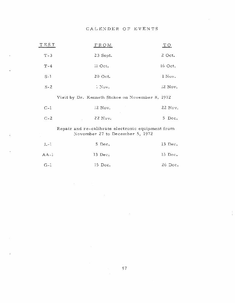
CALENDER OF EVENTS
TEST FROM TO
T-3 23 Sept. 2 Oct.
T-4 11 Oct. 16 Oct,
S-l 20 Oct. 1 Nov.
S-2 1 Nov. 12 Nov.
Visit by Dr. Kenneth Stokoe on Novelllber 8, 1972
C-l 12 Nov. 22 Nov.
C-2 22 Nov. S Dec.
Repair and re- calibra te electronic equiplllent frolllNovelllber 27 to Decelllber 5, 1972
L-l
AA-l
G-l
S Dec.
13 Dec.
15 Dec.
57
13 Dec.
15 Dec.
26 Dec.

TEST DESCRIPTIONS
TEST T-3: The test specimen was silty, medium BBC. An
attempt to measure volume changes using a burette and a backpressure
equal to 10 PSI did not work. At effective cell pressures greater than
25 PSI the consolidation data appeared as though there was a leak in
the membrane due to air diffusion (see Chapter III). The dynamic
test was run at the estimated in situ horizontal effective stress, then
the vertical, and then in 20 PSI increments up to 95 PSI. The specimen
was then unloaded in several steps, performing the dynamic test at
each step. Note that water was sucked into the sample during rebound
and this, combined with air dHfusion, caused problems during rebound,
The rebound values of C s reported in Figure 4.1 were taken after
flushing water through the porous stone.
TES T T -4: This test was on a specimen from the same tube
as Test T-3. The purpose of this test was to determine the repro
ducibility of C s performing the test in this manner; therefore, this
test was performed in the same manner as Test T-3, with essentially
the same results. Note however, that during the test, higher (than
expected) resonant frequencies were observed, but when the apparatus
was allowed to vibrate for a few minutes, these frequencies would
diminish to the expected values. Upon dismantling the apparatus at
the end of the te st a magnet wa s found to be dislodged from its proper
58

place. With further investigation, the higher frequencies could be
reproduced by shifting the magnet to and fro such that when it was in
the proper place the correct frequency was obtained, but when it wa s
not, the higher frequency was found. The magnet was then reglued to
its proper position and the calibration of the equipment checked.
TESTS S-l and S- 2: These tests were performed on specimens
of medium BBC with many silt lenses using the same testing procedure
as the T tests. Once again there was the problem of air diffusion,
which appeared to be leakage on the consolidation time plots. This is
evident in the rebound (unloading) curve in Figure 4.4 in which there
is some question as to whether the appropriate effective stress is
plotted.
TESTS C-l and C-2: These tests were run taking C s data
with tiTne to produce C s vs. Log time plots. This was suggested by
Stokoe and utilized to give a feel for what happens during consolidation.
An attempt was made to perform these tests at a shear strain of 1 x
10 - 5 in/in, but the AC noise in the electronic equipment interfered
with the accelerometer output. Therefore, the electronic equipment
was repaired and re-calibrated. Test C-l was run at different cell
pressures (Figure 4.2) to try to correlate these results with the
results of the previous tests. Test C-2 was run only at the in situ
effective octahedral stress due to a time limitation.
59

TEST L-l: This test was run at a small shear strain obtaining
C s vs. time for several consolidation pressures. The test consistently
showed the linear trend of C s vs. Log time in secondary consolidation.
It also showed that consistent results of C s (resonant frequency) CQuld
be obtained if the specimen was kept wet by flushing water through the
porous stone daily. 1£ the filter strips were allowed to dry due to air
diffusion, then this procedure resulted in a decrease in C s ' Therefore,
the author suggests flushing water through the porous stone daily. An
attempt was made to supply a reservoir of water at atmospheric pres
sure, but this did not work. The air had to be forced out of the stone
by pumping water through.
TEST AA-l: This test was performed only at the in situ
effective octahedral str es s on a specimen of soH, normally consoli,.;
dated BBC with a one inch sand layer in the middle. This sand layer
contained particles up to 1/4 inch. The results of C s vs. Log time
are shown in Figure 4. 6.
TEST G-l: This test wa s performed in essentially the sam_e
manner as Test AA-l, except a backpressure of 30 PSI was used.
The specimen was medium BBC with little silt. The results of the
first day of testing are illustrated in Figure 4.5. An attem-pt was made
to determine long term (time) effects, but air diffusion (see Chapter HI)
gave rise to erratic results after the fourth day of testing.
60

LIST OF REFERENCES
Chute, N. E., "Glacial Geology of the Mystic Lakes -- Fresh PondArea, Massachusetts", USGS Bulletin 106l-F, pp. 187-216,
1959.
Edgers, L., liThe Effect of Simple Shear Stress System on theStrength of Saturated Clay", thesis presented to MIT in 1967in partial fulfillment of the requirements for the degree ofMa ster of Science.
Hardin, Bobby 0., "Suggested Methods of Test for Shear Modulusand Damping of Soils by the Resonant Column! I , ASTM STP479, pp. 516-529, 1970.
Hardin, Bobby 0., and Black, W. L., !'Vibration Modulus of NormallyConsolidated Clay", Journal of Jhe Soil Mechanics and Foundations Division, ASCE, Volume 94, SM 2, March, 1968.
Hardin, Bobby 0., and Drnevich, V. P., "Shear Modulus and Dampingin Soils: Measurement and Parameter Effects", Journal ofthe Soil Mechanics and Foundations Division, ASCE, Volume98, SM 6, June, 1972.
Hardin, Bobby 0., and Mossbarger, W. A., Jr., !IThe ResonantColumn Technique for Vibration Testing of Soils and Asphalts",Proceedings, Instrument Society of America, October, 1966.
Hardin, Bobby 0., and Music, J., II Apparatus for Vibration Duringthe Triaxial Test", ASTM STP 392, June, 1965.
Ladd, C. C., and Luscher, U., II Engineering Properties of the SoilsUnderlying the MIT Campus", MIT Research Report R65-58,Soil Mechanics Publication # 185, December, 1965.
Ladd, R. S., "Use of Electrical Pressure Transducers to MeasureSoil Pressure", Research in Earth Physics, Phase Report# 5, MIT Dept. of Civil Engineering, Research Report R65-48,Soils Publication # 180, 1965.
61
Lambe, T. W., ?oil Testing for Engineers, J. Wiley & Sons,New York, 1951.
Marcuson, W. F., III, and Wahls, H. E., "Time Effects on DynamicShear Modulus of Clays", Journal of the Soil Mechanics andFoundations Division, ASCE, Volume 98, SM 12, December,1972.
Richart, F. E., Jr., Hall, J. R., Jr., and Woods, R. D., Vibrationsof Soils and Foundations, Prentice-Hall, New Jersey, 1970.
Seed, H. B., and Idris s, 1. M., "Influence of Soil Conditions onGround Motions During Earthquakes", Journal of the SoilMechanics and Foundations Division, ASCE, Volume 95,SM 1, January, 1969.
Stokoe, K. H., II, II Dynamic Response of Embedded Foundations",thesis presented to the University of Michigan in 1972 inpartial fulfillment of the requirements for the degree ofDoctor of Philosophy (Civil Engineering).
Whitman, R. V., and Richart, F. E., Jr., "Design Proceduresfor Dynamically Loaded Foundations", .;[ournal of the Soil.Mechanics and Foundations Division, ASCE, Volume 93,SM 6, November, 1967.
62


