

The Surprisingly Swift Decline of U.S.
Manufacturing Employment
Justin R. Pierce and Peter K. Schott∗
Abstract
This paper links the sharp drop in U.S. manufacturing employment
after 2000 to a change in U.S. trade policy that eliminated potential tar-
i� increases on Chinese imports. Industries more exposed to the change
experience greater employment loss, increased imports from China and
higher entry by U.S. importers and foreign-owned Chinese exporters.
At the plant level, shifts toward less labor-intensive production and ex-
posure to the policy via input-output linkages also contribute to the
decline in employment. Results are robust to other potential explana-
tions of employment loss, and there is no similar reaction in the EU,
where policy did not change. (JEL F13, F16, F61, F66, J23)
∗Pierce: Board of Governors of the Federal Reserve System, 20th & C Streets NW,Washington, DC 20551, [email protected]. Schott: Yale School of Management andNBER, 165 Whitney Avenue, New Haven, CT 06511, [email protected]. Schott thanksthe National Science Foundation (SES-0241474 and SES-0550190) for research support. Wethank Lorenzo Caliendo, Teresa Fort, Kyle Handley, Gordon Hanson, Amit Khandelwal,Mina Kim, Marc Muendler, Stephen Redding, Dan Tre�er and seminar participants at nu-merous institutions for helpful comments. We also thank Jonathan Ende, Rebecca Hammerand Deepra Yusuf for helpful research assistance. Any opinions and conclusions expressedherein are those of the authors and do not necessarily represent the views of the U.S. Cen-sus Bureau, the Board of Governors or its research sta�. All results have been reviewed toensure that no con�dential information is disclosed. The authors declare that they have norelevant or material �nancial interests that relate to the research described in this paper.

U.S. manufacturing employment �uctuated around 18 million workers be-
tween 1965 and 2000 before plunging 18 percent from March 2001 to March
2007. This paper �nds a link between this sharp decline and the U.S. granting
of Permanent Normal Trade Relations (PNTR) to China, which was passed
by Congress in October 2000 and became e�ective upon China's accession to
the World Trade Organization (WTO) at the end of 2001.1
Conferral of PNTR was unique in that it did not change the import tari�
rates the United States actually applied to Chinese goods over this period. U.S.
imports from China had been subject to the relatively low NTR tari� rates re-
served for WTO members since 1980.2 But for China, these low rates required
annual renewals that were uncertain and politically contentious. Without re-
newal, U.S. import tari�s on Chinese goods would have jumped to the higher
non-NTR tari� rates assigned to non-market economies, which were originally
established under the Smoot-Hawley Tari� Act of 1930. PNTR removed the
uncertainty associated with these annual renewals by permanently setting U.S.
duties on Chinese imports at NTR levels.
Eliminating the possibility of sudden tari� spikes on Chinese imports may
have a�ected U.S. employment through several channels. First, it increased
the incentive for U.S. �rms to incur the sunk costs associated with shifting
operations to China or establishing a relationship with an existing Chinese
producer.3 Second, it similarly provided Chinese producers with greater in-
1Though this paper focuses on the impact of a particular U.S. trade policy, it relates toa substantial body of research documenting a negative relationship between import compe-tition and U.S. manufacturing employment, including Freeman and Katz (1991), Revenga(1992), Sachs and Shatz (1994) and Bernard, Jensen and Schott (2006), as well as studieslinking Chinese imports to employment outcomes by Autor, Dorn and Hanson (2013), Utarand Torres Ruiz (2013), Bloom, Draca and Van Reenen (2015), Ebenstein et al. (2011),Groizard, Ranjan and Rodriguez-Lopez (2012) and Mion and Zhu (2013).
2Normal Trade Relations is a U.S. term for the familiar principle of Most Favored Nation.3A New York Times article reporting on the passage of PNTR noted the link to uncer-
tainty: �U.S. companies expect to bene�t from billions of dollars in new business and an
2

centives to invest in entering or expanding into the U.S. market, increasing
competition for U.S. producers. Finally, for U.S. producers, it boosted the
attractiveness of investments in capital- or skill-intensive production technolo-
gies or less labor-intensive mixes of products that are more consistent with
U.S. comparative advantage. Intuition for these channels of adjustment can
be derived from the large literature on investment under uncertainty, where
�rms are more likely to undertake irreversible investments as the ambiguity
surrounding their expected pro�t decreases.4
We quantify the transition from annual to permanent normal trade rela-
tions via the �NTR gap,� de�ned as the di�erence between the non-NTR rates
to which tari�s would have risen if annual renewal had failed (which average
37 percent in 1999) and the NTR tari� rates that were locked in by PNTR
(which average 4 percent in 1999). Importantly, the NTR gap exhibits sub-
stantial variation across industries: in 1999, its mean and standard deviation
are 33 and 14 percentage points. Larger responses are expected in industries
with higher NTR gaps.
Our generalized di�erence-in-di�erences identi�cation strategy exploits this
cross-sectional variation in the NTR gap to test whether employment in man-
end to years of uncertainty in which they had put o� major decisions about investing inChina� (Knowlton 2000). Section A below and Section A of the online appendix containadditional anecdotes describing the e�ect of PNTR-related uncertainty on U.S. and Chinese�rms' behavior.
4The e�ect of uncertainty on investment can be positive or negative depending upon arange of �rm and market characteristics, including adjustment costs, product market compe-tition and production technology. The negative association between PNTR and employmentfound here is consistent with a range of theoretical (e.g., Rob and Vettas 2003) and empirical(e.g,. Guiso and Pirigi 1999, Bloom, Bond and Van Reenen 2007) applications. A theoreti-cal framework closely related to our setting is Pindyck (1993), which shows that uncertaintyover input costs increases the value of waiting before undertaking sunk investments. Forexample, using this framework, Schwartz and Zozaya-Gorostiza (2003) show that input costuncertainty lowers incentives to invest in new information technology. Handley (2014) andHandley and Limao (2014, 2015) show that reduction in destination-country trade policyuncertainty is associated with increased entry into exporting.
3

ufacturing industries with higher NTR gaps (�rst di�erence) is lower after the
change in policy relative to employment in the pre-PNTR era (second di�er-
ence). An attractive feature of this approach is its ability to isolate the role
of the change in policy. While industries with high and low gaps are not iden-
tical, comparing outcomes within industries over time isolates the di�erential
impact of China's change in NTR status.
Regression results reveal a negative relationship between the change in U.S.
policy and subsequent employment in manufacturing that is both statistically
and economically signi�cant. The baseline speci�cation implies that moving an
industry from an NTR gap at the 25th percentile of the observed distribution
to the 75th percentile increases the implied relative loss of employment by 0.08
log points.
The relationship between PNTR and U.S. manufacturing employment re-
mains statistically and economically signi�cant after controlling for policy
changes in China associated with its accession to the WTO that may be spu-
riously correlated with the NTR gap, including a reduction in import tari�s,
the phasing out of export licensing requirements and production subsidies,
and the elimination of barriers to foreign investment. Furthermore, the results
are robust to controlling for other U.S. economic developments contempora-
neous with PNTR, such as the bursting of the 1990s information technology
bubble, the expiration of the global Multi-Fibre Arrangement governing Chi-
nese textile and clothing export quotas, and declining union membership in
the United States. To further verify that the U.S. reaction can be attributed
to the change in U.S. policy, we compare U.S. employment before and after
PNTR to that in the European Union, which gave China the equivalent of
PNTR much earlier, in 1980. We �nd no relationship between the U.S. NTR
gap and EU manufacturing employment after the U.S. granting of PNTR to
4

China.
We use data from a range of sources to explore the potential mechanisms
behind the U.S. response. Using U.S. trade data, we �nd that PNTR is asso-
ciated with relative increases in the value of U.S. imports from China as well
as the relative number of U.S. importers, Chinese exporters and U.S.-China
importer-exporter pairs. These outcomes demonstrate that U.S. imports from
China surge in the high-NTR gap products most a�ected by PNTR, suggesting
that the decline in U.S. employment is due in part to substitution of Chinese
imports for U.S. output. They also o�er a deeper understanding of the impact
of reducing uncertainty in international trade. That is, while our �nding of
a positive association between the NTR gap and Chinese exporters is consis-
tent with models of exporting under trade policy uncertainty5, the surge in
U.S. importers and U.S.-importer and Chinese-exporter pairs found here high-
lights a rich set of potential responses among �rms in the importing country,
e.g., within-�rm o�shoring. Toward that end, we use Chinese microdata to
show that PNTR is associated with a relative increase in Chinese exports to
the United States among foreign-owned Chinese �rms, and U.S. microdata to
demonstrate that PNTR is associated with a relative increase in the number of
U.S. and Chinese �rms engaged in related party trade. Each of these outcomes
is consistent with within-�rm relocation of U.S. production to China.
Additional insight into possible mechanisms explaining our main result
comes from examining U.S. outcomes at the plant level. Comparison of plant
employment and plant death regressions reveals that some plants were able
to adapt to the change in U.S. policy rather than die. Further analysis of
5Handley and Limao (2015) note that their framework could be used to examine a linkbetween PNTR and China's export boom, and Handley and Limao (2014) examine such alink using product-level trade data.
5

surviving plants' factor usage shows that PNTR is associated with increased
capital intensity, a reaction that is consistent with two mechanisms of trade-
induced adaptation: changes in product composition (as in Khandelwal 2010)
and adoption of labor-saving technologies (as in Bloom, Draca and Van Reenen
2015), with the latter suggesting that PNTR may be associated with employ-
ment reductions beyond those attributable to replacement of U.S. production
by Chinese imports. Finally, we �nd that employment among continuing plants
and plant survival respond negatively to exposure to PNTR in downstream
(customer) industries, providing indirect evidence of the sort of trade-induced
supply-chain disruptions modeled by Baldwin and Venables (2013).
The paper proceeds as follows: Section 1 describes our data, Section 2
describes our empirical strategy and main results, Sections 3 and 4 present
additional results, and Section 5 concludes. An online appendix provides ad-
ditional empirical results as well as information about dataset construction
and sources.
I Data
A Measuring the E�ect of PNTR: The NTR Gap
A.1 Policy Background
U.S. imports from non-market economies such as China are subject to rel-
atively high tari� rates originally set under the Smoot-Hawley Tari� Act of
1930. These rates, known as �non-NTR� or �column 2� tari�s, are often sub-
stantially larger than the �NTR� or �column 1� rates the United States o�ers
fellow members of the WTO. However, the U.S. Trade Act of 1974 allows
the President of the United States to grant NTR tari� rates to non-market
6

economies on an annually renewable basis subject to approval by the U.S.
Congress, and U.S. Presidents began granting such waivers to China annually
in 1980.
While these waivers kept the tari� rates applied to Chinese goods low, the
need for annual approval by Congress created uncertainty about whether the
low tari�s would continue, particularly after the Tiananmen Square incident
in 1989. In fact, the U.S. House of Representatives introduced and voted on
legislation to revoke China's temporary NTR status every year from 1990 to
2001. These votes succeeded even in 1990, 1991 and 1992, but China's status
was not overturned because the U.S. Senate failed to sustain the House votes.
From 1990 to 2001, the average House vote against annual NTR renewal was
38 percent.6
Anecdotal evidence indicates that Congressional threats to withdraw China's
NTR status were taken seriously. Media reports, Congressional testimony and
government reports make clear that �rms viewed renewal of China's NTR
status as uncertain, and that this uncertainty suppressed investment needed
to source goods from China. Indeed, in a 1994 report by the U.S. General
Accounting O�ce (U.S. GAO), U.S. �rms �cited uncertainty surrounding the
annual renewal of China's most-favored-nation trade status as the single most
important issue a�ecting U.S. trade relations with China� and indicated that
�uncertainty over whether the U.S. government will withdraw or place further
conditions on the renewal of China's most-favored-nation trade status a�ects
the ability of U.S. companies to do business in China� (U.S. GAO 1994). These
�ndings echoed a letter to President Clinton from the CEOs of 340 �rms, in-
cluding General Motors, IBM, Boeing, McDonnell Douglas and Caterpillar, in
which they stated that �[t]he persistent threat of MFN withdrawal does little
6Table A.1 of the online appendix summarizes the House votes by year.
7

more than create an unstable and excessively risky environment for U.S. com-
panies considering trade and investment in China, and leaves China's booming
economy to our competitors� (Rowley 1993). Moreover, the anecdotes under-
score the idea that uncertainty can have a chilling e�ect on investment even
if the probability of rescinding NTR is low. Testifying before the House Ways
and Means Committee, a representative from Mattel asserted that �[w]hile
the risk that the United States would withdraw NTR status from China may
be small, if it did occur the consequences would be catastrophic for U.S. toy
companies given the 70 percent non-MFN U.S. rate of duty applicable to toys�
(St. Maxens 2000).7 After passage of PNTR, the Congressional Commission
created to track its e�ects reported that: �In the months since the enactment
of PNTR legislation with China there has been an escalation of production
shifts out of the U.S. and into China...[B]etween October 1, 2000 and April
30, 2001 more than eighty corporations announced their intentions to shift
production to China, with the number of announced production shifts increas-
ing each month from two per month in October to November to nineteen per
month by April� (U.S. Trade De�cit Review Commission 2001).
Uncertainty associated with annual renewals of China's NTR status is
also apparent in a simpli�ed version of the well-known Baker, Bloom and
Davis (2015) policy uncertainty index, which we calculate to relate speci�cally
to China's NTR renewals. In constructing this index, a research assistant
searched the database Proquest for articles that contain the words �China,�
�uncertain� or �uncertainty,� and �most favored nation� or �normal trade rela-
tions,� for the years 1989 to 2013. The search was limited to articles in The
Wall Street Journal, The New York Times, and The Washington Post, and
7Additional anecdotes are provided in Section A of the online appendix.
8

irrelevant articles were manually screened from the search results.8 Following
Baker, Bloom and Davis (2015), article counts are summed by year and then
divided by the total number of articles produced by the three newspapers. The
resulting index is displayed in Figure 1. As shown in the �gure, the policy un-
certainty index spikes in periods of tension in U.S.-China relations, with the
highest levels observed in the early 1990s after Tiananmen Square and in 2000
during the debate over PNTR.9 After passage of PNTR in 2000, the index goes
essentially to zero indicating that uncertainty regarding China's NTR status
was e�ectively resolved.
[Note: Location of Figure 1 approximately here]
The U.S. Congress passed a bill granting PNTR status to China in October
2000 following the November 1999 agreement between the United States and
China governing China's eventual entry into WTO. PNTR became e�ective
upon China's accession to the WTO in December 2001, and was implemented
on January 1, 2002.10 The baseline analysis in Section II treats years from
2001 forward as being �post-PNTR.� Alternate speci�cations in Section B re-
lax this assumption by allowing the relationship between the NTR gap and
employment to di�er in each year.
The change in China's PNTR status had two e�ects. First, it ended the
uncertainty associated with annual renewals of China's NTR status, thereby
eliminating any option value of waiting for U.S. or Chinese �rms seeking to
8A list of the articles included in the index as well as those that were screened outmanually is available from the authors upon request.
9Additional peaks occur around the time of China's transfer of missile technology toPakistan (1993) and the Taiwan Straits Missile Crisis (1996).
10While each of these milestones likely contributed to the overall reduction in policyuncertainty, both the anecdotal evidence and the policy uncertainty index described aboveindicate that passage of PNTR in 2000 played a key role in the elimination of uncertaintyfor U.S. �rms.
9

incur sunk costs associated with greater U.S.-China trade.11 Second, it led to a
substantial reduction in expected U.S. import tari�s on Chinese goods. We dis-
cuss channels through which the change in policy a�ected U.S. manufacturing
employment in Section IV.
A.2 Calculating the NTR Gap
We quantify the impact of PNTR on industry i as the di�erence between the
non-NTR rate to which tari�s would have risen if annual renewal had failed
and the NTR tari� rate that was locked in by PNTR,
(1) NTR Gapi = Non NTR Ratei −NTR Ratei,
and we expect industries with larger NTR gaps to be more a�ected by the
change in U.S. policy. One attractive feature of this measure is its plausible
exogeneity to employment after 2000. Seventy-nine percent of the variation
in the NTR gap across industries arises from variation in non-NTR rates, set
70 years prior to passage of PNTR. This feature of non-NTR rates e�ectively
rules out reverse causality that would arise if non-NTR rates could be set to
protect industries with declining employment. Furthermore, to the extent that
NTR tari�s were set to protect industries with declining employment prior to
PNTR, these higher NTR rates would result in lower NTR gaps, biasing our
results away from �nding an e�ect of PNTR.
We compute NTR gaps using ad valorem equivalent NTR and non-NTR
11To our knowledge, no other U.S. trade policy generates similar uncertainty with respectto China. For example, while the the Omnibus Trade and Competitiveness Act of 1988requires the U.S. Treasury Secretary to provide semiannual reports indicating whether anymajor trading partner of the United States is manipulating its currency, such a designa-tion only requires the Secretary to initiate negotiations to have the exchange rate adjusted�promptly� (U.S. Department of the Treasury 2012).
10

tari� rates from 1989 to 2001 provided by Feenstra, Romalis and Schott (2002).
Both types of tari�s are set at the eight-digit Harmonized System (HS) level,
also referred to as �tari� lines.� We compute industry-level NTR gaps using
concordances provided by the U.S. Bureau of Economic Analysis (BEA); the
gap for industry i is the average NTR gap across the eight-digit HS tari� lines
belonging to that industry. Further detail on the construction of NTR gaps is
provided in Section B.1 of the online appendix.
We use the NTR gaps for 1999 � the year before passage of PNTR in
the United States � in our regression analysis, but note that the baseline
results are robust to using the NTR gaps from any available year (see Section
B). Furthermore, the baseline empirical speci�cation explicitly controls for
industries' NTR rates. In 1999, the average NTR gap across industries is 0.33
with a standard deviation of 0.14, and its distribution is displayed in Figure
2. The corresponding statistics are 0.04 and 0.07 for the NTR rate and 0.37
and 0.16 for the non-NTR rate.
[Note: Location of Figure 2 approximately here]
B U.S. Manufacturing Employment
Our principal source of data is the U.S. Census Bureau's Longitudinal Business
Database (LBD), assembled and maintained by Jarmin and Miranda (2002).
These data track the employment and major industry of virtually every es-
tablishment with employment in the non-farm private U.S. economy annually
as of March 12.12 In these data, �establishments� correspond to facilities in
12The LBD de�nition of employment includes both full- and part-time workers; in SectionC we show that our main employment results are robust to examining production hoursinstead of employment. While the use of sta�ng services by manufacturing �rms wasincreasing during the 2000s, Dey, Houseman and Polivka (2012) show that this trend doesnot account for the steep decline in manufacturing employment after 2000.
11
a given geographic location, such as a manufacturing plant or retail outlet,
and their major industry is de�ned at the four-digit Standard Industrial Clas-
si�cation (SIC) or six-digit North American Industry Classi�cation System
(NAICS) level. Longitudinal identi�ers in the LBD allow establishments to be
followed over time.
The long time horizon considered in this paper presents two complications
for analyzing the evolution of manufacturing employment. The �rst compli-
cation is that the industry classi�cation scheme used to track establishments'
major industries changes from the SIC to the NAICS in 1997 and to subse-
quent versions of NAICS in 2002 to 2007. Because we need time-consistent
industry de�nitions to track employment over our sample period, we use the
algorithm developed in Pierce and Schott (2012a) to create �families� of four-
digit SIC and six-digit NAICS codes that are linked through the SIC and
NAICS industry classi�cation systems. Further detail on the creation of time-
consistent industry codes is provided in Section B.3 of the online appendix.
Unless otherwise noted, all references to �industry� in this paper refer to these
families.
The second complication is that some activities (e.g., logging and publish-
ing) are re-classi�ed out of �manufacturing� in the SIC to NAICS transition
and, moreover, some plants are sometimes classi�ed within manufacturing
and sometimes outside manufacturing. We construct a �constant manufactur-
ing sample� that excludes any families that contain SIC or NAICS industries
that are ever classi�ed outside manufacturing. In addition, we exclude any
plants that are ever classi�ed outside manufacturing. Use of this constant
manufacturing sample ensures that our results are not driven by any changes
in classi�cation system.13 We note, however, that qualitatively identical re-
13The results are also robust to use of a beta version of time-consistent NAICS codes
12
sults can be obtained using the simple NAICS manufacturing de�nition in the
publicly available NBER-CES Manufacturing Industry Database from Becker,
Gray and Marvakov (2013), and that neither of these drops has a material im-
pact on the general trend of manufacturing employment over the past several
decades.14
While the loss of U.S. manufacturing employment after 2000 is dramatic,
we note that it is not accompanied by a similarly steep decline in value added.
Indeed, as illustrated in Figure 3, real value added in U.S. manufacturing, as
measured by the BEA, continues to increase after 2000, though at a slower rate
(2.8 percent) compared with the average from 1948 to 2000 (3.7 percent).15
[Note: Location of Figure 3 approximately here]
C Data for Alternate Explanations
We consider a wide array of alternate explanations for the observed decline
in U.S. manufacturing employment. To be plausible, these alternate explana-
tions must explain why the decline in employment coincides with the timing
of PNTR and why it is concentrated in industries most a�ected by the policy
change. Descriptions and sources of the data used to capture these explana-
tions are presented in Section D of the online appendix. Here, we provide
a brief overview of the three classes of alternate explanations we consider: a
decline in the U.S. competitiveness of labor-intensive goods, policy changes in
China, and other notable macroeconomic events in the United States.
developed for the LBD by Teresa Fort and Shawn Klimek.14Section B.3 of the online appendix compares annual employment in our �constant�
manufacturing sample against the manufacturing employment series available publicly fromthe U.S. Bureau of Labor Statistics. Both display a stark drop in employment after 2000.
15Houseman et al. (2011) argue that gains in manufacturing value-added in the lateryears of Figure 3 may be overstated as purchases of low-cost foreign materials are not fullycaptured in input price indexes.
13
U.S. manufacturing employment may have fallen after 2000 due to a decline
in the competitiveness of U.S. labor-intensive industries for some reason other
than the change in U.S. trade policy, such as a general movement towards
o�shoring encouraged by the 2001 recession or a positive productivity shock
in labor-abundant China.16 We control for these explanations by including
measures of industry capital and skill intensity in our speci�cation and by
allowing the impact of these industry factor intensities to vary before and
after PNTR.
As part of its accession to the WTO, China agreed to institute a number of
policy changes which could have in�uenced U.S. manufacturing employment,
including liberalization of its import tari� rates, export licensing rules, produc-
tion subsidies and barriers to foreign investment. We control for these policy
changes using data on Chinese import tari�s from Brandt et al. (2012), data
on export licensing requirements from Bai, Krishna, and Ma (2015), and data
on production subsidies from China's National Bureau of Statistics. Because
China's reduction of barriers to foreign investment may have a�ected indus-
tries di�erently based on the nature of contracting in their industry, we also
include Nunn's (2007) measure of the proportion of intermediate inputs that
require relationship-speci�c investments.
Finally, the granting of PNTR to China overlaps with several notable events
in the United States. The �rst was the abolishment of import quotas on some
textile and clothing imports in 2002 and 2005 under the global Multi-Fibre
Arrangement (MFA). The second was the bursting of the U.S. tech �bubble�
and the subsequent recovery. A third is a steady decline in unionization in
16We show in Section E of the online appendix that China's TFP growth is uncorrelatedwith the NTR gap. Furthermore, we demonstrate in Section 4 that the EU does not ex-perience a similar decline in manufacturing employment in high NTR gap industries after2000.
14

the manufacturing sector. We control for the potential impact of these events
using data on U.S. textile and clothing quotas from Khandelwal, Schott and
Wei (2013), de�nitions of advanced technology products posted on the U.S.
Census Bureau's website, and industry-level unionization rates from Hirsch
and Macpherson (2003).
Table A.2 of the online appendix summarizes the relationships between the
NTR gap and the industry-level control variables we employ in the baseline
speci�cation, described in greater detail below. The strongest relationship
among these variables is a negative relationship with capital intensity (R2 =
0.23).
II PNTR and U.S. Manufacturing Employment
A Baseline Speci�cation
We examine the link between PNTR and U.S. manufacturing employment
using a generalized OLS di�erence-in-di�erences (DID) speci�cation that ex-
amines whether employment losses in industries with higher NTR gaps (�rst
di�erence) are larger after the imposition of PNTR (second di�erence). In-
dustry �xed e�ects capture the impact of any time-invariant industry char-
acteristics, and year �xed e�ects account for aggregate shocks that a�ect all
industries equally. The sample includes annual industry-level data from 1990
to 2007.
We estimate the following equation:
15

ln(Empit) = θPostPNTRt ×NTR Gapi +(2)
γPostPNTRt ×Xi + λXit +
δt + δi + α + εit,
where the dependent variable is the log level of employment in industry i in
year t. The �rst term on the right hand side is the DID term of interest,
an interaction of the NTR gap and an indicator for the post-PNTR period,
i.e., years from 2001 forward. The second term on the right hand side is an
interaction of the post-PNTR dummy variable and time-invariant industry
characteristics, such as initial year (1990) industry capital and skill intensity
or the degree to which industries encompass high-technology products. This
term allows for the possibility that the relationship between employment and
these characteristics changes in the post-PNTR period. The third term on
the right-hand side of equation 2 captures the impact of time-varying industry
characteristics, such as exposure to MFA quota reductions, union membership
and the NTR tari� rate.17 δi, δt and α represent industry and year �xed e�ects
and the constant. Regressions are weighted by industry employment in 1990.
Results are reported in Table 1 with robust standard errors clustered by
industry. The �rst column includes only the DID term and the necessary
�xed e�ects, while the second column adds industry initial factor intensities.
The third column includes all covariates capturing the e�ect of the alternate
17NTR tari� rates from Feenstra, Romalis and Schott (2002) are unavailable after 2001and so are assumed constant after that year. As discussed in Section B, we obtain nearlyidentical results using analogously computed �revealed� tari� rates from public U.S. tradedata for all years but use the Feenstra, Romalis and Schott (2002) measures because theyare available for a larger set of industries.
16

explanations discussed in Section C and represents the �baseline� speci�cation
to which we refer throughout the remainder of the paper.
As indicated in the �rst row of Table 1, estimates of θ are negative and
statistically signi�cant in all speci�cations, indicating that the imposition of
PNTR coincides with lower manufacturing employment. Moving across the
columns from left to right shows that the estimate for θ decreases in absolute
value as additional covariates are added, but remains statistically signi�cant
at conventional levels.
The estimated e�ects are also economically signi�cant. The di�erence-
in-di�erences coe�cient in the baseline speci�cation in column 3 indicates
that moving an industry from an NTR gap at the 25th (0.23) to the 75th
percentile (0.40) of the observed distribution increases the implied relative
loss of employment by -0.08 (=-0.47*(0.40-0.23)) log points. We also perform
a two-step calculation of the implied impact of PNTR that takes into account
the employment weights of industries across the distribution of NTR gaps.
First, for each industry i, we multiply θ by the industry's NTR gap. This
yields an implied e�ect of PNTR (versus the pre-period) on employment for
each industry relative to a hypothetical industry with a zero NTR gap. Second,
we average the implied relative e�ects for all manufacturing industries, using
initial industry employment as weights. As reported in the �nal row of the
third column of the table, the baseline speci�cation implies a relative decline
in manufacturing employment of -0.15 log points.18
18Though our di�erence-in-di�erences identi�cation strategy precludes estimation of theoverall share of employment lost to the change in U.S. policy, we note that several prominentstudies of the impact of trade liberalization on manufacturing employment have found largee�ects. Autor, Dorn and Hanson (2013), using an alternate means of identi�cation, �ndthat depending on assumptions used to isolate the Chinese supply shock, Chinese importpenetration explains 26 to 55 percent of the overall decline in U.S. manufacturing employ-ment from 2000 to 2007, or -5 to -11 percentage points of the overall -20 percent decline. Ina di�erent setting, Tre�er (2004) �nds that the Canada-U.S. Free Trade Agreement reduced
17

The remaining rows of the third column of Table 1 display a positive and
statistically signi�cant relationship between employment and industries' ini-
tial skill intensity (de�ned as the ratio of non-production workers to total
employment), and negative and statistically signi�cant relationships between
employment and industries' exposure to tari� reductions in China and MFA
quota reductions.19 The positive coe�cient for skill intensity indicates that
skill-intensive industries more in line with U.S. comparative advantage do rel-
atively well in terms of employment after 2000. The negative point estimate
on exposure to Chinese import tari�s reveals that U.S. employment rises in
relative terms in industries where Chinese import tari�s decline. The negative
coe�cient for MFAExposureit indicates that textile and clothing industries
more exposed to the elimination of quotas experience greater relative employ-
ment loss.20
[Note: Location of Table 1 approximately here]
Canadian manufacturing employment by 12 percent among industries in the top tercile ofimport tari� declines, i.e. those with an average reduction of -10 percent. Moreover, thegrowth in Chinese exports to the U.S. during our sample period dwarfs that of U.S. exportsto Canada during the period studied by Tre�er (2004). According to the U.S. InternationalTrade Commission website, Chinese exports to the United States grew by $223 billion from2000 to 2007 (from $100 billion to $323 billion), while U.S. exports to Canada grew by $44billion between 1989 and 1996 (from $75 billion to $119 billion), in nominal terms.
19As discussed further in Section D.3 of the online appendix, the negative and statisticallysigni�cant relationship between PNTR and manufacturing employment is also robust tosimply dropping industries that contain products subject to the MFA.
20Following Brambilla, Khandelwal and Schott (2009), we measure the extent to whichindustries' quotas were binding under the MFA as the import-weighted average �ll rate of thetextile and clothing products that were under quota, where �ll rates are de�ned as the actualimports divided by allowable imports under the the quota. Industries containing textile andclothing products with higher �ll rates faced more binding quotas and are therefore morelikely to experience employment reductions when quotas are eliminated. Fill rates are set tozero for unbound products. See Section D.3 of the online appendix for additional informationregarding construction of the MFA variable.
18

B Robustness and Extensions
This section assesses the the timing and linearity assumptions inherent in the
baseline speci�cation, the exogeneity of the NTR gap, and the sensitivity of
our results to alternate controls for business-cycle �uctuations and an alternate
measure of tari�s.
Timing : For the decline in employment to be attributable to PNTR, our
policy measure, the NTR gap, should be correlated with employment after
PNTR, but not before. To determine whether there is a relationship be-
tween the NTR gap and employment in the years before 2001, we replace the
PostPNTR indicator used in equation 2 with interactions of the NTR Gap
and the full set of year dummies,
ln(Empit) =2007∑
y=1991
(θy1{y = t} ×NTR Gapi) +2007∑
y=1991
(βy1{y = t} ×Xi)(3)
+λXit + δt + δi + α + εit.
As above, we estimate equation 3 both with and without the industry controls.
Results for the di�erence-in-di�erences coe�cients, θy, are displayed visu-
ally along with their 90 percent con�dence intervals in Figure 4, as well as
numerically in Table A.4 of the online appendix. Coe�cient estimates for the
remaining covariates are omitted to conserve space. As indicated in both the
�gure and the table, point estimates are statistically insigni�cant at conven-
tional levels until after 2001, at which time they become statistically signi�cant
and increasingly negative.21 This pattern is consistent with the parallel trends
21Results are similar for an event study version of this speci�cation that compares out-comes across years for industries in the top versus bottom quintiles of the NTR gap distri-bution.
19

assumption inherent in our di�erence-in-di�erences analysis, lending further
support for the baseline empirical strategy.
[Note: Location of Figure 4 approximately here]
Exogeneity : Though nearly all of the variation in the NTR gap arises from
non-NTR rates set in 1930, and increases in NTR rates to protect declin-
ing industries would result in smaller NTR gaps, we examine two alternate
speci�cations designed to evaluate the exogeneity of the NTR gaps. First,
we estimate a two-stage least squares speci�cation in which we instrument
the baseline DID term, PostPNTRt × NTR Gapi, with an interaction of
the post-PNTR indicator and the Smoot-Hawley-based non-NTR tari� rates,
PostPNTRt ×NNTRi. As indicated in the �rst column of Table 2, the DID
term remains negative and statistically signi�cant, with a magnitude some-
what larger in absolute value than that in our baseline result. Second, we
re-estimate our baseline speci�cation (equation 2) using the NTR gap ob-
served in 1990, ten years prior to PNTR. As shown in column 2 of Table 2, the
DID coe�cient estimate remains negative and statistically signi�cant, with a
magnitude somewhat larger than that of our baseline result.
Non-Linearity : We estimate two non-linear speci�cations to determine
whether the NTR gap has less of an e�ect on �rms' employment decisions
beyond some threshold level or, alternatively, whether the e�ect of the NTR
gap grows disproportionately as it increases with higher values of the NTR gap.
The �rst augments equation 2 with the interaction of the square of the NTR
gap with the 1{PostPNTRt} dummy. The second constrains the relationship
between employment and the NTR gap to be a two-segment spline.22 Re-
22The spline is estimated using a constrained OLS regressions that restricts the post-PNTR relationship between employment and the NTR gap to be two successive line segmentsstarting at the origin and joined at a �knot.� We grid over NTR gap knots in incrementsof 0.05 and report the speci�cation that minimizes the Akaike Information Criterion (AIC),
20

sults are reported in columns three and four of Table 2. P-values testing the
joint signi�cance of the di�erence-in-di�erences coe�cients in the quadratic
speci�cation and implied economic signi�cance, computed using the two-step
procedure as noted above, are reported in the �nal two rows of the table. In
addition, Figure A.2 in the online appendix plots the relationship between the
DID terms and log employment implied by each speci�cation over the range
of NTR gaps observed in the data.
As indicated in both the table and the �gure, the results provide some
support for the idea that employment loss accelerates with the NTR gap. On
the other hand, column 3 of Table 2 reveals that while the coe�cients for the
NTR gap terms in the quadratic speci�cation are jointly statistically signi�cant
at conventional levels, the square term is not itself statistically signi�cant.
In terms of economic signi�cance, the nonlinear speci�cations yield economic
impacts comparable to that implied by the baseline linear speci�cation. The
quadratic speci�cation yields a relative decline in manufacturing employment
of -0.12 log points and the spline speci�cation yields a relative decline of -0.16
log points, compared to -0.15 log points in the baseline linear speci�cation.
Business cycles : We estimate two alternate speci�cations that control ex-
plicitly for the potential in�uence of business cycle �uctuations on employ-
ment.23 The �rst adds interactions of capital and skill intensity with real
GDP, indexed to a base year of 1990, to our baseline speci�cation (equation
2). The second follows Tre�er (2004) by including industry-year-speci�c pre-
reported in the penultimate row of Table 2. Minimization of Schwarz's Bayesian InformationCriterion yields identical results.
23To the extent that aggregate shocks a�ect all industries equally, their e�ect on employ-ment is captured by the year �xed e�ects included in equation 2. Furthermore, includinginteractions of initial capital and skill intensity with the full set of year dummies when esti-mating equation 3 allows for annual aggregate shocks to have di�erential e�ects on industriesbased on variation in those industry characteristics.
21

dictions of the the change in employment associated with growth in U.S. real
GDP and the U.S. real e�ective exchange rate, as well as one and two-period
lags of growth in these two variables. As shown in columns �ve and six of Table
2, inclusion of these additional business-cycle controls has little e�ect on our
DID coe�cient estimate either in terms of statistical or economic signi�cance.
Revealed Tari�s : We re-estimate equation 2 using a measure of revealed
tari�s in place of the applied NTR rates used in the baseline speci�cation.
We calculate ad valorem equivalent revealed NTR tari� rates by summing the
duties collected for each eight-digit HS product by year and dividing this sum
by the corresponding dutiable value. These revealed tari� measures capture
changes in tari� rates due to NAFTA and other preferential trade agreements.
As shown in column seven of Table 2, using these revealed tari� data does not
lead to any material change in the statistical or economic signi�cance of our
results.24
[Note: Location of Table 2 approximately here]
III The United States versus the EU
Comparison of outcomes in the United States versus the European Union
provides an alternate test of the idea that PNTR drives the employment
decline in the United States. In contrast to the United States, the Euro-
pean Union granted permanent most-favored-nation status to China in 1980
(Casarini 2006). As a result, there was little change in either the actual or
expected EU tari�s on Chinese goods when the U.S. granted PNTR to China
in 2000, and imports from China were not subject to the annual potential
24As noted above, the revealed tari� data are available for fewer industries than arecovered in the Feenstra, Romalis and Schott (2002) data. As a result, the the number ofobservations for this regression is reduced.
22

tari� increases present in the United States.25 Comparing the United States
and the EU therefore helps determine whether U.S. NTR gaps are spuriously
correlated with other factors that may have a�ected employment in both the
United States and EU, such as technological change, policy changes in China
related to its entry to the WTO, or positive Chinese productivity shocks.
Our comparison makes use of data from the United Nations Industrial De-
velopment Organization's (2013) INDSTAT 4 dataset, which tracks employ-
ment by country and four-digit International Standard Industrial Classi�ca-
tion (ISIC) industries from 1997 to 2005.26 We estimate a triple di�erence-in-
di�erences speci�cation that examines employment for industries with varying
NTR gaps (�rst di�erence) after the imposition of PNTR (second di�erence)
and across the United States and the EU (third di�erence):27
ln(Empict) = θPostPNTRt ∗NTR Gapi ∗ USc(4)
+δct + δci + δit + α + εict.
The dependent variable is log employment for four-digit ISIC industry i in
25China was a Generalized System of Preferences (GSP) bene�ciary in the EU before andafter its accession to the WTO. According to European Commission (2003), Chinese importtari�s under the EU GSP program did not change when it joined the WTO. The EU renewsGSP every decade and conducts annual revisions to their rates. These changes are generallymade on a product-by-product rather than country-by-country basis, suggesting that theyare not biased towards China. Nevertheless, we note that the majority of the EU's GSPrate changes in recent years involve products in which Chinese exporters are active.
26The four-digit ISIC industries across which employment is reported are more aggregatedthan either the SIC or NAICS industries across which U.S. employment data is reportedin the LBD. We aggregate NTR gaps to the six-digit HS level and then map them to thefour-digit ISIC level using publicly available concordances from the World Bank. See sectionF of the online appendix for additional information regarding the UNIDO data.
27Data for the EU member countries are aggregated to the EU level, so that the regressionincludes observations for two �countries,� the United States and the European Union. SeeSection F of the online appendix for additional information regarding these data.
23

c ∈ US,EU in year t. θ is the coe�cient for the triple-di�erence term of
interest where USc is an indicator variable that takes the value one for the
United States. δct, δci and δit represent country×year, country×industry and
industry ×year �xed e�ects. α is the regression constant.
Results are reported in the �rst column of Table 3, with robust standard
errors clustered by country×industry. As shown in the �rst row of the table,
θ is negative and statistically signi�cant, indicating that PNTR is associated
with a relative decline in manufacturing employment in the United States
versus the EU. Separate di�erence-in-di�erence speci�cations for the the EU
and the United States (columns 2 and 3) provide complementary evidence:
PNTR is associated with statistically signi�cant employment declines in the
United States but not the EU.28
The results in Table 3 are evidence against the idea that post-PNTR em-
ployment loss in the United States is due to an unobserved shock a�ecting
manufacturing employment globally, or a shock in China that a�ects its ex-
ports to the U.S. and EU equally. They also con�rm the relationship between
employment and the NTR gap for the United States using an entirely di�erent
dataset and industrial classi�cation system for employment.
[Note: Location of Table 3 approximately here]
28The results for the United States using UNIDO data in column 3 of Table 3 are com-parable to those using U.S. Census data in column 1 of Table 1. In both cases, the pointestimates for the DID term are negative and statistically signi�cant, and they are of similarmagnitude despite the use of di�erent datasets. The substantially smaller number of obser-vations in column 3 of Table 3 versus column 1 of Table 1 is due to the shorter time intervalavailable in the UNIDO data (1997 to 2005 versus 1990 to 2007) as well as the fact thatindustry de�nitions in the UNIDO data are broader than those used by the U.S. Census.
24

IV Potential Mechanisms
PNTR may have caused a decline in U.S. manufacturing employment via sev-
eral mechanisms, including: (1) encouraging U.S. �rms to start sourcing inputs
or �nal goods from Chinese rather than domestic suppliers; (2) persuading Chi-
nese �rms to expand into the U.S. market; (3) motivating U.S. manufacturers
either to invest in labor-saving production techniques or to produce more skill-
and capital-intensive products that are more in line with U.S. comparative ad-
vantage; and (4) inducing U.S. �rms to shift all or part of their operations
o�shore, perhaps in conjunction with other �rms in their supply chains. In
this section we provide evidence consistent with all of these mechanisms.
A U.S. Imports
Given that PNTR entailed a change in U.S. trade policy vis-a-vis China, we
examine whether it was associated with changes in U.S. imports from China
versus other countries. As noted in the introduction, relative growth in Chinese
imports could be due to U.S. �rms sourcing goods from China, the expansion
of Chinese exporters or o�shoring by U.S. manufacturers.
We use customs data from the U.S. Census Bureau's Longitudinal For-
eign Trade Transaction Database (LFTTD). As described in greater detail in
Bernard, Jensen and Schott (2009), the LFTTD tracks all U.S. international
trade transactions beginning in 1992. For each import transaction we observe
the product traded, the U.S. dollar value and quantity shipped, the shipment
date and the origin country. The data also contain codes identifying both the
U.S. importer and the foreign supplier of the imported product.
We employ a generalized triple di�erences speci�cation that compares prod-
ucts with varying NTR gaps (�rst di�erence) before and after PNTR (second
25

di�erence) and across source countries (third di�erence) for the years 1992 to
2007:
Ohct = θ1{c = China}c × PostPNTRt ×NTR Gaph +(5)
+λTariffhct + δct + δch + δht + α + εhct.
The left-hand side variable represents the log level of one of several dimensions
of U.S. import activity aggregated to the eight-digit HS product by source
country by year level.29 These dimensions are import value, the number of
U.S. �rms importing product h from country c in year t, the number of country
c �rms exporting product h to the United States in year t, and the number of
importer-exporter pairs engaged in U.S. imports of product h from country c
in year t. The �rst term on the right-hand side is the primary term of interest:
a triple interaction of an indicator for China, an indicator for the post-PNTR
period, and the NTR gap for product h. Its coe�cient, θ, captures the impact
of the change in U.S. policy. Tariffhct represents the U.S. revealed import
tari� for product h from country c in year t, computed as the ratio of duties
collected to dutiable value using publicly available U.S. trade data. δct, δch and
δht represent country×year, country×product and product×year �xed e�ects.
α is the regression constant.30
Results are reported in Table 4, with robust standard errors clustered at the
country×product level. Estimates of θ are positive and statistically signi�cant
for all four dimensions of U.S. importing. As indicated in the bottom row of
29As with SIC and NAICS industries, the eight-digit HS product codes are linked totime-invariant families using the concordance from Pierce and Schott (2012a).
30Although this speci�cation omits observations where the left-hand side variable is equalto zero, we note that similar results are obtained in a previous version of this paper (Pierceand Schott 2012b) when examining changes in those variables normalized as suggested byDavis, Haltiwanger and Schuh (1996).
26

the table, these estimates imply that PNTR raises the relative import value
of the a�ected products by 0.17 log points vis a vis imports of those products
from other sources after the change in U.S. policy. The analogous responses
for the number of U.S. importers, the number of Chinese exporters and the
number of importer-exporter pairs are 0.15, 0.17 and 0.17 log points.
These results demonstrate that U.S. import value from China surges in the
high-NTR-gap products most a�ected by PNTR, suggesting that the decline
in U.S. employment is due in part to substitution of Chinese imports for U.S.
output, either due to growth of Chinese exporters or o�shoring/outsourcing by
U.S. manufacturers.31 Moreover, the relative increases in both the number of
U.S. importers and the number of Chinese exporters are consistent with U.S.
and Chinese �rms being more willing to undertake irrecoverable investment in
establishing bilateral trade relationships after PNTR, in line with the broad
literature on investment under uncertainty. Relative to the existing literature
on trade policy uncertainty (Handley 2014, Handley and Limao 2014, 2015),
which focuses on exporting, the results with respect to U.S. importers highlight
the potential importance of reactions to uncertainty by �rms in the importing
country.32 We pursue these reactions further in the next section.
[Note: Location of Table 4 approximately here]
31Our �ndings relate to Harrison and McMillan (2011), who show that o�shore employ-ment in low-wage countries is a substitute for domestic employment among U.S. manufac-turers.
32Handley and Limao (2014) discusses welfare implications of eliminating trade policyuncertainty for the importing country, via the price index, but does not consider adjustmentsby �rms in the importing country, such as o�shoring.
27

B O�shoring of Production by U.S. Firms
One way in which PNTR could lead to employment declines in the U.S. is via
o�shoring, in which U.S. �rms locate production in China that would otherwise
occur in the United States. We �nd evidence consistent with o�shoring by
U.S. �rms using both Chinese data tracking the exports of Chinese �rms and
additional U.S. trade data that classi�es U.S. imports according to whether
they take place between arm's-length or related parties.
B.1 Evidence from Chinese Exports
We �rst examine whether PNTR is associated with changes in the pattern of
Chinese exports using �rm-level customs data from China's National Bureau
of Statistics (NBS) provided by Khandelwal, Schott and Wei (2013).33 One
advantage of these Chinese export data vis a vis the U.S. import data is the
ability to classify Chinese exporters as domestic versus foreign-owned. As a
result, they can shed light on whether China's surge in high-NTR-gap exports
to the United States may be due to o�shoring by foreign �rms versus market
expansion by Chinese �rms. Translated anecdotes from Chinese language news
accounts provided in Section A.2 of the online appendix o�er support for both
of these channels. For example, Shanghai Securities News noted in 1999 that if
China's accession to the WTO led to PNTR being granted: �...[T]his will help
to build con�dence among investors at home and abroad, especially among
United States investors, because currently, China faces the issue every year of
maintaining Most Favored Nation trading status (Shanghai Securities News
33The Chinese data track China's exports by �rm, product, destination, country, andyear from 2000 to 2005. For each �rm-product-destination-year observation, we observe thenominal value of exports shipped as well as codes for the ultimate ownership of the �rm andthe type of export shipment.
28

1999).�
Following Khandelwal, Schott and Wei (2013), we use the ownership codes
to classify �rms into three groups: state-owned enterprises (�SOEs�), privately
owned domestic �rms (�domestic�) and privately owned foreign �rms (�for-
eign�).34 In addition, we decompose overall exports into �general� versus �pro-
cessing & assembling� (�P&A�), where the latter refers to goods produced with
intermediate inputs imported tari�-free on the condition that they not be sold
domestically.35
We examine the e�ect of PNTR on Chinese exports using the same triple
di�erences speci�cation used for the U.S. import data above (equation 5), but
with two di�erences. First, we replace the indicator for China as a source of
imports with an indicator for the United States as a destination for exports.
Second, we aggregate the Chinese data to the six-digit HS level in order to
assign NTR gaps, as U.S. and Chinese product codes are not consistent at
more disaggregated levels. Coe�cient estimates and robust standard errors
clustered by country×product are reported in Table 5.
The �rst column of the Panel A presents results for all �rms and all trade
types, and the positive and statistically signi�cant coe�cient indicates that
PNTR is associated with an increase in Chinese exports to the U.S., relative
to other countries. This result complements and con�rms the trade e�ects
reported in Section A using an independent dataset. That is, where the U.S.
data indicate that U.S. imports from China relative to other sources increase
with the change in U.S. policy, the Chinese data show that Chinese exports
to the United States increase relative to other destinations with the change in
34SOEs include collectives, and foreign �rms include joint ventures.35General and P&A exports account for more than 95 percent of exports in each year of
the sample. Other export categories are omitted. Across the years for which the data areavailable, general exports represent approximately 43 percent of total exports.
29

U.S. policy.
Examining results by �rm type, we �nd the strongest relationship between
PNTR and exports among foreign-owned �rms (column 4). Indeed, for these
�rms, higher NTR gaps are associated with increases in relative exports to
the United States for both general exports (Panel B) and P&A exports (Panel
C). While the country of foreign ownership is not reported in the NBS data,
to the extent that some portion of these exporters are a�liates of U.S. �rms,
the results are consistent with o�shoring by U.S. producers following PNTR.36
Coe�cient estimates for SOEs and privately owned domestic �rms, while also
positive for both types of exports, are generally statistically insigni�cant at
conventional levels.
[Note: Location of Table 5 approximately here]
B.2 Evidence from U.S. Related Party Importers
We further investigate the potential role of o�shoring within �rms using data
on U.S. imports between related parties. A shift of domestic production by
U.S. manufacturers to new or newly acquired a�liates in China in response to
PNTR could result in an increase in related-party imports of products with
higher NTR gaps from China, vis a vis other countries. We examine this mech-
anism using the �related-party� �ag present in the U.S. import data, which
36Noisy data on U.S. �rms' overseas employment posted on the BEA's website providesome support for this interpretation, though it should be treated with caution. Available forseven highly aggregate manufacturing sectors, these data track U.S. multinationals' employ-ment in their overseas a�liates by country and year on a consistent basis starting in 1999,though 18 percent of cells are imputed or suppressed to protect con�dential information.Nevertheless, using a triple di�erences speci�cation similar to equation 5, we �nd that PNTRis associated with a relative increase in overseas manufacturing employment after PNTR,though the coe�cient estimate is not statistically signi�cant at conventional levels (p-value0.27). The seven sectors are: food; chemicals; primary and fabricated metals; machinery;computers and electronic products; electrical equipment, appliances and components; andtransportation equipment.
30

indicates whether the U.S. importer and the foreign exporter are �related� by
ownership of at least 6 percent.37
Using the same speci�cation (equation 5) employed in Section A, we �nd
in Table 6 that higher NTR gaps are associated with statistically signi�cant
increases in the number of U.S. importers sourcing imports from related-parties
in China, the number of Chinese exporters exporting to a related-party in the
United States, and the number of related-party importer-exporter pairs. The
relationship with respect to value, while positive, is not statistically signi�cant
at conventional levels, though we note that this lack of signi�cance appears
to be driven by a lag between the formation of the related-party importer-
exporter pairs and the imports that �ow between them.38 Overall, these results
indicate a relative increase in the number of Chinese a�liates from which U.S.
�rms source goods in response to PNTR, consistent with an expansion of
o�shoring activity.
[Note: Location of Table 6 approximately here]
C Inducing Changes in U.S. Factor Intensity
PNTR may have a�ected U.S. manufacturing employment not only through
the substitution of imports from China for U.S. production, but also by induc-
ing �rms facing increased import competition to decrease employment through
37Growth of related-party trade is just one potential manifestation of o�shoring. Forexample, it does not include the growth in trade associated with �rms that produced andsold to arm's-length customers in the United States prior to PNTR but that subsequentlymoved production to China while continuing to sell to their previous customers.
38For example, consideration of an alternate speci�cation focusing on long di�erences �i.e., comparison of related party import growth in the six years prior to PNTR to thatin the six years after PNTR � reveals a positive and statistically signi�cant relationshipbetween the NTR gap and Chinese export growth to the United States, post-PNTR. Thisspeci�cation is similar to that estimated in an earlier version of this paper, Pierce and Schott(2012b): 4ln(Ohct:t+6) = θ1{c = China}c × PostPNTRt × NTR Gaph + λTariffhct +δct + δch + δht + α+ εhct, where t ∈ {1995, 2001} .
31

adjustment of their production processes or product mix. To examine this pos-
sibility, we analyze the relationship between PNTR and factor usage � i.e., skill
and capital intensity � using quinquennial data collected in the U.S. Census of
Manufactures (CM). We perform this analysis at both the industry and plant
level to determine the extent to which changes in factor intensity are driven
by entry and exit versus changes within continuing plants.39
For years ending in �2� and �7�, the CM contains plant characteristics in-
cluding total employment, a breakdown of total employment into production
and non-production workers, production worker hours and capital.40 As in
Section II we de�ne skill intensity as the ratio of non-production workers to
total employment and capital intensity as the ratio of capital to total employ-
ment. Our analysis makes use of the same generalized di�erence-in-di�erences
speci�cation de�ned in equation 2, with one important di�erence: because
the CM tracks establishments' attributes only every �ve years, the pre-PNTR
period is de�ned as 1992 and 1997 and the post-PNTR period is de�ned as
2002 and 2007.
We �rst present industry-level results in Table 7 that capture adjustments
due to entry and exit of plants with di�erent factor intensities, as well as
changes within continuing plants. As indicated in Columns 1 and 2 of the table,
PNTR is associated with statistically and economically signi�cant increases in
both industry skill intensity and industry capital intensity. The gain in skill in-
tensity arises from heterogeneous responses for the two types of workers tracked
in our data. While we �nd negative and statistically signi�cant relationships
39Holmes and Stevens (2014) show that increased import competition from China canhave heterogeneous e�ects among plants within an industry, with the biggest negative e�ectobserved at large plants producing standardized goods. Small plants producing specialtygoods are less a�ected.
40Real book value of capital is de�ated using industry-level investment price indexes fromBecker, Gray and Marvakov 2013.
32

between employment and the NTR gap for both non-production (column 3)
and production workers (column 4), the implied impact of PNTR for pro-
duction workers is more than one and a half times that for non-production
workers. This result is consistent with research (e.g., Ebenstein et al. 2014)
�nding that the e�ect of import competition on wages is concentrated among
production workers engaged in routine blue-collar production occupations.41
As indicated in column 6, the gains in capital intensity arise from statistically
signi�cant declines in total employment (column 5) compared to a statistically
insigni�cant response for capital (column 6).42
[Note: Location of Table 7 approximately here]
Next, we examine the extent to which the increases in industry-level capital
and skill intensity associated with PNTR are driven by changes within con-
tinuing plants. Estimates from a series of plant-level regressions are reported
in Table 8, with robust standard errors clustered by plants' major industry.
These regressions di�er from the industry-level regressions in two ways. First,
they make use of plant-level NTR gaps, de�ned as the weighted-average NTR
gap across all of the industries in which the plant is active in 1997. Second,
they contain plant �xed e�ects as well as plant-level control variables such
as age and total factor productivity in addition to the industry-level control
variables used in the baseline speci�cation.43
41Results in column 7 show that the PNTR-related decline in production hours is similarin magnitude to that for total employment, ruling out the possibility that the decline inemployment resulted from a contraction on the extensive margin (the number of employees)that was o�set by an expansion on the intensive margin (the number of hours per worker).
42Results for total employment in column 5 are similar in terms of both statistical andeconomic signi�cance to those reported in the baseline speci�cation in Section II, despiteuse of a di�erent dataset.
43We follow Foster, Haltiwanger and Syverson (2008) in measuring TFP as the log ofde�ated revenue minus the log of inputs, weighted by the average cost share for each inputacross industries (see Section B.4 of the online appendix for more detail). We note thatproductivity measures constructed from revenue information may be biased due to unob-
33

Results in the �rst two columns of Table 8 indicate that while PNTR is not
associated with changes in skill intensity for continuing plants, it is associated
with capital deepening. Indeed, as noted in the �nal row of column 2, the im-
plied economic impact of PNTR on plant capital intensity is a relative increase
of 0.09 log points. This relative capital deepening within plants is consistent
with two mechanisms of employment loss: trade-induced technological change,
as in Bloom, Draca and Van Reenen (2015), and trade-induced product up-
grading, as in Bernard, Jensen and Schott (2006), Khandelwal (2010), and
Schott (2003, 2008), with the former suggesting that PNTR may be associ-
ated with employment reductions beyond those attributable to replacement of
U.S. production by Chinese imports.44
[Note: Location of Table 8 approximately here]
D Input-Output Linkages
PNTR may also a�ect employment at U.S. manufacturing plants indirectly
via their supply chains, i.e., the upstream �rms from which they purchase
their inputs or the downstream �rms to which they sell their outputs. Indeed,
recent theoretical research by Baldwin and Venables (2013) suggests that re-
ductions in trade frictions for one portion of the supply chain may lead to
co-o�shoring of its suppliers and customers, leading to large, discontinuous o�-
served establishment-level variation in prices, which can be a�ected by changes in tradepolicy (Pierce 2011 and De Loecker et al. 2015).
44We provide anecdotal evidence supporting these mechanisms in Section A.3 of the onlineappendix. For example: �To beat the Chinese and other foreign competitors threatening[their] business, [the owners] invested several million dollars to double the production ca-pacity of their plastic-part plant, PM Mold, with the latest in robotics and automationequipment. Now, [it] can make twice as many parts � and better ones at that � withoutadding to [its] work force (Neikirk 2002).�
34

shoring events.45 In this sense, input-output linkages may amplify the negative
relationship between PNTR and manufacturing employment, serving as im-
portant mechanism for the policy's e�ect. Alternatively, plants bene�ting from
greater access to lower-priced Chinese inputs might expand operations relative
to others whose input suppliers are less exposed to PNTR. More generally, a
number of recent papers emphasize the importance of examining input-output
linkages when estimating the impact of import competition, e.g. Amiti and
Konings (2007), Goldberg et al. (2010), Acemoglu et al. (2014) and Razhev
(2015).
We examine the transmission of PNTR through input-output linkages by
computing plant-level up- and downstream NTR gaps using information from
the BEA input-output tables and including them in a plant-level regression:
Opt =∑m
θmd PostPNTRt ×NTR Gapmp(6)
+γPostPNTRt ×Xi + λ×Xit + µXpt
+δt + δp + α + εpt,
where Opt represents either log employment of continuing plant p in year t or
an indicator variable that takes a value of 1 if the plant dies between year
t and year t + 1 and 0 otherwise. NTR Gapmp represents the NTR gap for
m = {Own,Upstream,Downstream}; for each dependent variable, we report
estimates for speci�cations that both exclude and include the up- and down-
stream NTR gaps.46 All speci�cations use the annual plant-level data available
45Ellison, Glaeser and Kerr (2010), for example, �nd that proximity to suppliers andcustomers is an important determinant of the location of manufacturing activity.
46Section B.1 of the appendix provides a detailed description of calculation of the plant-level up- and downstream NTR gaps.
35

from the LBD.
Results in Table 9 provide evidence that PNTR's e�ect on employment can
be transmitted, and potentially magni�ed, through supply chains. Columns
one and three, which do not control for supply-chain linkages, indicate that
higher exposure to PNTR in plants' own industry is associated with lower
employment within continuing plants and a higher probability of plant death.
By comparison, the results in columns two and four show that plants whose
customers are more exposed to PNTR � as measured by the downstream NTR
gap � also contract employment and are more likely to die.47 This e�ect via
downstream industries is consistent with either a contraction in output when
plants' customers face negative demand shocks, or to co-o�shoring as plants
relocate to China to be closer to their customers. More generally, the results
show that PNTR a�ects U.S. manufacturing employment along both the inten-
sive and extensive margins, by reducing employment within continuing plants
and by inducing plant exit.48
[Note: Location of Table 9 approximately here]
V Conclusion
This paper �nds a relationship between the sharp decline in U.S. manufac-
turing employment after 2000 and the United States' conferral of permanent
47In terms of economic signi�cance, the impact of PNTR implied by the results in column2 is a relative -0.14 log point decline in employment in the post-PNTR period, with theown and downstream NTR gaps contributing roughly equally. Computation of economicsigni�cance excludes the impact of the statistically insigni�cant coe�cient for the upstreamNTR gap.
48The working version of this paper, Pierce and Schott (2012b), shows that anemic jobcreation accounts for approximately one quarter of the overall estimated impact of PNTR,with the remainder due to exaggerated job destruction. These trends provide a partial ex-planation for the post-2000 shift in job creation and destruction rates discussed in Faberman(2008).
36

normal trade relations on China, a policy that is notable for eliminating the
possibility of future tari� increases � and the uncertainty with which they were
associated � rather than reducing the tari�s actually applied to Chinese goods.
We measure the e�ect of PNTR as the gap between the the high non-NTR
rates to which tari�s would have risen if annual renewal of China's NTR sta-
tus had failed and the lower NTR tari� rates that were locked in by PNTR.
Using a generalized di�erence-in-di�erences speci�cation, we show that indus-
tries with higher NTR gaps experience larger employment declines, along with
disproportionate increases in U.S. imports from China, the number of U.S.
�rms importing from China and the number of Chinese �rms exporting to the
United States, especially foreign-owned Chinese �rms. These results are robust
to inclusion of variables proxying for a wide range of alternate explanations
for the observed trends in employment and trade. Moreover, we demonstrate
that the pattern of employment losses in the United States � which experi-
enced the policy change � is not present in the European Union, which had
granted China the equivalent of PNTR status in 1980. Additional analysis
of the mechanisms by which the change in policy a�ected U.S. manufacturers
reveals evidence consistent with o�shoring by U.S. �rms, reallocation within
high-gap industries towards less labor-intensive plants, increases in the capital
intensity of the most a�ected plants, and magni�cation of the e�ects of PNTR
via downstream customers.
Having established a link between the change in trade policy and U.S.
employment outcomes, this research raises several important, but challenging
questions. To what extent can PNTR explain the diverging trends of value-
added and employment in the U.S. manufacturing sector? What impact did
PNTR have on U.S. prices and consumption patterns? To what extent did
U.S. �rms change the composition of their output in response to PNTR, and
37

how large were the associated transition costs? We hope to bring additional
data to bear on these questions in future research.
References
[1] Acemoglu, Daron, David Autor, David Dorn, Gordon H. Hanson and
Brendan Price. 2014. �Import Competition and the Great U.S. Employ-
ment Sag of the 2000s.� Journal of Labor Economics, forthcoming.
[2] Amiti, Mary and Jozef Konings. 2007. �Trade Liberalization, Intermediate
Inputs and Productivity.� American Economic Review 97 (5): 1611-38.
[3] Autor, David H., David Dorn and Gordon H. Hanson. 2013. �The China
Syndrome: Local Labor Market E�ects of Import Competition in the
United States.� American Economic Review 103 (6): 2121-68.
[4] Bai, Xue, Kala Krishna and Hong Ma. 2015. How You Export Matters:
Export Mode, Learning and Productivity in China.� NBER Working Pa-
per 21164.
[5] Baker, Scott R., Nicholas Bloom and Stephen J. Davis. 2015. �Measuring
Economic Policy Uncertainty.� NBER Working Paper 21633.
[6] Baldwin, Richard and Anthony J. Venables. 2013. �Spiders and Snakes:
O�-Shoring and Agglomeration in the Global Economy.� Journal of In-
ternational Economics 90 (1): 245-54.
[7] Becker, Randy, Wayne B. Gray and Jordan Marvakov. 2013.
�NBER-CES Manufacturing Industry Database.� Available at
www.nber.org/data/nberces5809.html.
[8] Bernard, Andrew B., J. Bradford Jensen, and Peter K. Schott. 2006. �Sur-
vival of the Best Fit: Exposure to Low-Wage Countries and the (Uneven)
Growth of US Manufacturing Plants.� Journal of International Economics
38

68 (1): 219-237.
[9] Bernard, Andrew B., J. Bradford Jensen and Peter K. Schott. 2009. �Im-
porters, Exporters and Multinationals: A Portrait of Firms in the U.S.
that Trade Goods.� In Producer Dynamics: New Evidence from Micro
Data, edited by Timothy Dunne, J. Bradford Jensen and Mark J. Roberts.
Chicago: University of Chicago Press.
[10] Bloom, Nick, Stephen Bond and John Van Reenen. 2007. �Uncertainty
and Investment Dynamics.� Review of Economic Studies 74(2007): 391-
415.
[11] Bloom, Nick, Mirko Draca and John Van Reenen. 2015. �Trade Induced
Technical Change: The Impact of Chinese Imports on Innovation, Di�u-
sion and Productivity.� Review of Economic Studies, forthcoming.
[12] Brambilla, Irene, Amit K. Khandelwal and Peter K. Schott. 2009. �China's
Experience Under the Multi�ber Arrangement (MFA) and the Agree-
ment on Textiles and Clothing (ATC).� In China's Growing Roll in World
Trade, edited by Robert Feenstra and Shang-Jin Wei. Chicago: University
of Chicago Press. Forthcoming.
[13] Brandt, Loren, Johannes Van Biesebroeck, Luhang Wang and Yifan
Wang. 2012. �WTO Accession and Performance of Chinese Manufacturing
Firms.� Center for Economic Policy Research Working Paper 9166.
[14] Bureau of Economic Analysis. 1948-2010. �Real Value Added:
Manufacturing.� United States Department of Commerce.
www.bea.gov/industry/gdpbyind_data.htm.
[15] Bureau of Labor Statistics. 1948-2010. �Current Employment Statis-
tics: National Manufacturing Employment, Not Seasonally Ad-
justed, CEU3000000001.� United States Department of Labor.
http://data.bls.gov/timeseries/CEU3000000001?data_tool=XGtable.
39

[16] Casarini, Nicola. 2006. �The Evolution of the EU-China Relationship:
From Constructive Engagement to Strategic Partnership.� Occasional Pa-
per Number 64, European Union Institute for Security Studies.
[17] Davis, Steven J., John C. Haltiwanger and Scott Schuh. 1996. Job Cre-
ation and Destruction. Cambridge: MIT Press.
[18] De Loecker, Jan, Pinelopi K. Goldberg, Amit K. Khandelwal and Nina
Pavcnik. 2015. �Prices, Markups and Trade Reform.� Econometrica, forth-
coming.
[19] Dey, Matthew, Susan N. Houseman and Anne E. Polivka. 2012. �Manu-
facturers' Outsourcing to Sta�ng Services.� Industrial & Labor Relations
Review 65 (3): 533-559.
[20] Ebenstein, Avraham, Margaret McMillan, Yaohui Zhao and
Chanchuan Zhang. 2011. �Understanding the Role of China in the
`Decline' of US Manufacturing.� www.margaretsmcmillan.com/wp-
content/uploads/2012/03/5_Ebenstein-et-al.-US-Manufacturing-and-
China-November-2011.pdf.
[21] Ebenstein, Avraham, Ann Harrison, Margaret McMillan and Shannon
Phillips. 2014. �Estimating the Impact of Trade and O�shoring on Ameri-
canWorkers Using the Current Population Surveys.� Review of Economics
and Statistics 96 (4): 581-595.
[22] Ellison, Glenn, Edward Glaeser, and William R. Kerr. 2010. �What
Causes Industry Agglomeration? Evidence from Coagglomeration Pat-
terns.� American Economic Review 100 (3): 1195�1213.
[23] European Commission. 2003. Overview of
the Terms of China's Accession to WTO.
http://trade.ec.europa.eu/doclib/docs/2003/october/tradoc_111955.pdf
[24] Faberman, R. Jason. 2008. �Job Flows, Jobless Recoveries and the Great
40

Moderation.� Federal Reserve Bank of Philadelphia Working Paper Num-
ber 08-11.
[25] Feenstra, Robert C., John Romalis and Peter K. Schott. 2002. �U.S. Im-
ports, Exports and Tari� Data, 1989-2001.� NBER Working Paper 9387.
[26] Foster, Lucia S., John C. Haltiwanger and Chad Syverson. 2008. �Re-
allocation, Firm Turnover and E�ciency: Selection on Productivity or
Pro�tability.� American Economic Review 98 (1): 394-425.
[27] Freeman, R., Katz, L., 1991. �Industrial Wage and Employment Determi-
nation in an Open Economy, in Immigration, Trade and Labor Market,�
edited by John M. Abowd and Richard B. Freeman. Chicago: University
of Chicago Press.
[28] Goldberg, Pinelopi, Amit Khandelwal, Nina Pavcnik and Petia Topalova.
2010. �Imported Intermediate Inputs and Domestic Product Growth: Ev-
idence from India.� Quarterly Journal of Economics 125 (4): 1727-67.
[29] Groizard, Jose L., Priya Ranjan and Jose Antonio
Rodriguez-Lopez. 2012. �Input Trade and Job Flows.�
www.bde.es/f/webpi/SES/seminars/2012/�les/sie1215.pdf.
[30] Guiso and Pirigi . 1999. �Investment and Demand Uncertainty.� Quarterly
Journal of Economics 114 (1): 185-227.
[31] Handley, Kyle. 2014. �Exporting Under Trade Policy Uncertainty: Theory
and Evidence.� Journal of International Economics 94 (1): 50-66.
[32] Handley, Kyle and Nuno Limao. 2014. �Policy uncertainty,
Trade and Welfare: Evidence from the U.S. and China.�
www.terpconnect.umd.edu/~limao/tpu_submitted.pdf.
[33] Handley, Kyle and Nuno Limao. 2015. �Trade and Investment under Pol-
icy Uncertainty: Theory and Firm Evidence.� American Economic Jour-
nal: Economic Policy 7 (4): 189-222.
41

[34] Harrison, Ann and Margaret McMillan. 2011. �O�shoring Jobs? Multina-
tionals and U.S. Manufacturing Employment.� The Review of Economics
and Statistics 93 (3): 857-875.
[35] Hirsch, Barry T. and David A. Macpherson. 2003. �Union Membership
and Coverage Database for the Current Population Survey.� Industrial
and Labor Relations Review 56 (2): 349-54.
[36] Holmes, Thomas J. and John J. Stevens. 2014. �An Alternative Theory
of the Plant Size Distribution with an Application to Trade.� Journal of
Political Economy 122 (2): 369-421.
[37] Houseman, Susan, Christopher Kurz, Paul Lengermann and Benjamin
Mandel. 2011. �O�shoring Bias in U.S. Manufacturing.� Journal of Eco-
nomic Perspectives 25 (2): 111-132.
[38] Jarmin, Ron and Javier Miranda. 2002. �The Longitudinal Business
Database.� Center for Economic Studies Discussion Paper CES-WP-02-
17.
[39] Khandelwal, Amit. 2010. �The Long and Short (of) Quality Ladders.�
Review of Economic Studies 77 (4), 1450-1476.
[40] Khandelwal, Amit K., Peter K. Schott and Shang-Jin Wei. 2013. �Trade
Liberalization and Embedded Institutional Reform: Evidence from Chi-
nese Exporters.� American Economic Review 103 (6): 2169-95.
[41] Kirkbride, Rob. 2001. �Furniture Makers Sink or Swim with the Foreign
Flood.� The Grand Rapids Press. April 29, 2001.
[42] Knowlton, Brian. 2000. �Final Passage of Bill to Normalize U.S. Ties is
Approved, 83 to 15: Senate Vote Introduces New Era in China Trade.�
The New York Times. September 20, 2000.
[43] Mion, Giordano and Like Zhu. 2013. �Import Competition From and Out-
sourcing to China: A Curse or a Blessing for Firms.� Journal of Interna-
42

tional Economics 89 (1): 202-215.
[44] Neikirk, William. 2002. �Abundance of Cheap Imports Hurts Economy.�
Chicago Tribune. December 17, 2002.
[45] Nunn, Nathan. 2007. �Relationship-Speci�city, Incomplete Contracts and
the Pattern of Trade.� Quarterly Journal of Economics 122 (2) 569-600.
[46] Pierce, Justin R. 2011. �Plant-Level Responses to Antidumping Duties:
Evidence from U.S. Manufacturers.� Journal of International Economics
85 (2): 369-378.
[47] Pierce, Justin R. and Peter K. Schott. 2012a. �Concording U.S. Harmo-
nized System Codes Over Time.� Journal of O�cial Statistics 28 (1):
53-68.
[48] Pierce, Justin R. and Peter K. Schott. 2012b. �The Surprisingly Swift De-
cline of U.S. Manufacturing Employment.� NBER Working Paper 18655.
[49] Pindyck, Robert S. 1993. �Investments of Uncertain Cost.� Journal of
Financial Economics 34 (1): 53-76.
[50] Razhev, Mark. 2015. �Input-Output Structure and Trade Elasticity.�
http://scholar.princeton.edu/sites/default/�les/razhev/�les/jmp_razhev.pdf.
[51] Revenga, A.L. 1992. �Exporting Jobs? The Impact of Import Competition
on Employment and Wages in U.S. Manufacturing.� Quarterly Journal of
Economics 107 (1): 255-284.
[52] Rob, Rafael and Nikolaos Vettas. 2003. �Foreign Direct Investment and
Exports with Growing Demand.� Review of Economic Studies 70(3): 629-
648.
[53] Rowley, Storer H. 1993. �China Woos Western Businesses, Snubs Clinton.�
Chicago Tribune. May 20, 1993.
[54] Sachs, J.D., Shatz, H.J. 1994. �Trade and Jobs in U.S. Manufacturing.�
Brookings Papers on Economic Activity 1994 (1): 1-69.
43

[55] Schott, Peter K. 2003. �One Size Fits All? Heckscher-Ohlin Specialization
in Global Production.� American Economic Review 93 (2): 686-708.
[56] Schott, Peter K. 2008. �The Relative Sophistication of Chinese Exports.�
Economic Policy 53: 5-49.
[57] Schwartz, Eduardo S. and Carlos Zozaya-Gorostiza. 2003. �Investment
Under Uncertainty in Information Technology: Acquisition and Develop-
ment Projects.� Management Science 49 (1): 57-70.
[58] Shanghai Securities News. 1999. �Outlook 2000.� Shanghai Securities
News. December 28, 1999.
[59] St. Maxens, Thomas F. 2000. Statement of Thomas F. St. Maxens, St.
Maxens and Company, on behalf of Mattel, Inc., El Segundo, CA. U.S.-
China Bilateral Trade Agreement and the Accession of China to the WTO.
Hearing before the Committee on Ways and Means, House of Represen-
tatives, One Hundred Sixth Congress, Second Session, February 16, 2000.
Washington: U.S. Government Printing O�ce.
[60] Tre�er, Daniel. 2004. �The Long and Short of the Canada-U.S. Free Trade
Agreement.� American Economic Review 94 (4): 870-895.
[61] United Nations Industrial Development Organiza-
tion. 2013. INDSTAT 4 Database. United Nations.
www.unido.org/resources/statistics/statistical-databases/indstat4-
2013-edition.html.
[62] U.S. Department of the Treasury. 2012. Report to Congress on Interna-
tional Economic and Exchange Rate Policies. www.treasury.gov/resource-
center/international/exchange-rate-policies/Documents/Foreign Ex-
change Report May 2012.pdf.
[63] United States General Accounting O�ce. 1994. U.S. Government Policy
Issues A�ecting U.S. Business Activities in China. Report to the Chair-
44
man, Committee on Government A�airs, and the Honorable Joseph I.
Lieberman, U.S. Senate.
[64] U.S. Trade De�cit Review Commission. 2001. �Impact of U.S.-
China Trade Relations on Workers, Wages and Employment.�
http://govinfo.library.unt.edu/tdrc/research/research.html
[65] Utar, Hale and Luis B. Torres Ruiz. 2013. �International Competition and
Industrial Evolution: Evidence form the Impact of Chinese Competition
on Mexican Maquiladoras.� Journal of Development Economics 105: 267-
287.
45

��������� ��������� ���������
��� ��������� ������ ��� ������ ��� ������ ���
����� ����� �����
��� ����������������� ����� ������
����� �����
��� ������������������ ��� � ����� ���
����� �����
��� �!��"�#��$��%�&�'� ���� �
�����
��� �∆!(&���$��"����"&))�� ������ �
�����
��� �∆!(&���*+,&-&%�� �����
���
��� �∆!(&���.&#%�&�/�� �����
�����
��� ��01-2��#%-��%#(��/'�3� ������
�����
451�� �+"%�� ������ ���
�����
������ ������
�����
6�*��6�&��4%�,%"(&��� ������
�����
7,%"2��&� �8��� �8��� �8���
�� ��� ��� ����
5& %-��))%#� &8� &8� &8�
����'�%���9%&/(�%- :% :% :%
$���&%-�$���#��)����� ������ ������ ������
��%;���,�%�"%�"��"%+���)�7.*�/%�%"��&<%-�-&))%"%�#%�&��-&))%"%�#%�"%/"%&�����(%�-%�%�-%���2�"&�,�%�
&��(%��/�)�&�-+�"'�'%�"�%���'�%�����-��(%�&�-%�%�-%���2�"&�,�%�"%�"%%��&�/��(%�%))%#��)������&��(%�
&��%"�#�&��)��(%�����/�����-�����������&�-&#��"���1--&�&����#��"��&�#�+-%��&�%�2�"'&�/�2�"&�,�%����451�
% �+"%8�������"&))�"��%8�+�&���%�,%"(&��"��%������=%�����&��%"�#�&��)��(%���������&�-&#��"�=&�(�
�&�%�&�2�"&����#��"��&�#�+-&�/��(%��/�)������#��&������-�>&���&��%�&�'8�#��"�#��&��%�&�'���+��������8�
#(��/%�&��!(&�%%�&��"����"&))8�#(��/%�&��!(&�%%��"-+#�&��+,&-&%8�#(��/%�&��!(&�%%�% �"���&#%�&�/�
"%?+&"%�%�����-����&�-&#��"�)"�=(%�(%"��(%�&�-+�"'��"-+#%��-2��#%-��%#(��/'��"-+#����@��������
���������������,+�����-�"-�%"""��-A+�%-�)"�#�+�%"&�/�����(%�&�-+�"'��&���%2%���"%�-&���'%-�,%�=�%�#(�
#%))&#&%������&���%�)"��(%�'%�"�������-�&�-+�"'�)& %-�%))%#����=%������(%�#�������"%�+��"%%-��
7,%"2��&���"%�=%&/(�%-�,'������&�-+�"'�%���'�%����5&����"=�"%�"���(%��"%-&#�%-�"%���&2%�#(��/%�&���(%�
-%�%�-%���2�"&�,�%�&���&%-�,'��(%�-&))%"%�#%�&��-&))%"%�#%�#%))&#&%����*+�%"#"&���BBB8�BB���-�B�"%�"%%���
���&�&#���&/�&)&#��#%�����(%��8�����-�����%"#%����%2%�����+�,%"�)�,%"2��&��(��,%%��"+�-%-����%�"%��
�(+��-�-+%���!%�+�C+"%�+�-&#�+"%��2&-��#%��"#%-+"%�
Table 1: Baseline Results (LBD)
46

��������� ��������� ��������� ��������� ��������� ��������� ���������
��� ��������� ������ ��� ������ ������ ��� ������ ��� ������ ���
����� ����� ����� ����� �����
��� �������������� ������ ���
�����
��� ����������
������
�����
��� �������������� ��� ������
�����
��� �����������!�� "# ����� �����
�����
��� �������������� ��� ������
�����
��� ����$%����������� ������ ������ ������ ����� �� ������ ��� ������ ������
���� ����� ����� ����� ����� ����� �����
��� ������%����������� ���� ��� ����� ��� ����� ��� ������ � ����� ��� ����� ��� ����� ���
���� ����� ����� ����� ����� ����� �����
��� �&��"�#��!�� �'�(� ����� � ������ ������ ����� � ������ ������ ������
���� ����� ����� ����� ����� ����� �����
��� �∆&)'���!��"����"'**�� ����� � ������ �� ������ � ������ ������ � ������ � ������
���� ����� ����� ����� ����� ����� �����
��� �∆&)'����+,'-' �� ����� ����� ����� ������ ��� ����� ����� ������
����� ����� ����� ����� ����� ����� �����
��� �∆&)'���.'# �'�/�� ������ ������ ������ ������ �� ������ ������ ������ �
����� ����� ����� ����� ����� ����� �����
��� ��01-2��# -�� #)��/(�3� ���� ������ ������ ����� ������ ������ ������
����� ����� ����� ����� ����� ����� �����
451�� �+" �� ���� ��� ������ ��� ������ ��� ������ ��� ������ ��� ������ ��� ������ ���
����� ����� ����� ����� ����� ����� �����
������ ������ ������ ������ ������ � ������ ������
����� ����� ����� ������ ����� �����
6����6�'��4 �, ")'��� ������ ������ ������ ������ � ������ ������ ������
���� ����� ����� ����� ����� ����� �����
�����7���� ����$%����������� �����
�����
�����7���� ������%����������� ������
�����
�" *� "�8+'� �&(#� �� �������
�����
� 2 �� -�����������
�
�����
9, "2��'� �:��� �:��� �:��� �:��� �:��� �:��� �:���
�� ���� ���� ���� � ���� ���� ����
��'���'� ��.� 9.� 9.� 9.� 9.� 9.� 9.�
!��"+� ��� �������� � � � � � �
5' -��** #� ':� ':� ':� ':� ':� ':� ':�
����(� ���; '/)� - < < < < < < <
='����'/�'*'#��# ���>��+ � � ����� ����� � � �
&��"�'� -���'���'�? � � � < � � �
$�� � � � ���� � � �
1!& � � � ����� � � �
!���' -�!���#��*����� ������ ������ ������ ������ ������ ������ ������
�� @���,� �" �"��" +���*�9.��/ � "��'A -�-'** " �# �'��-'** " �# �" /" '��*��/�'�-+�"(� ���(� ������� -�
� "�+���'��*����'�� "�#�'��*��) �����/���B'�)����'�-'#��"�*"��) ���������� "'-��1--'�'����#��"��'�#�+- ��'� �
2�"('�/�2�"'�,� ����451� �+" :�������"'**�"�� :�+�'��� �, ")'��"�� ������B �����'�� "�#�'��*��) ���������'�-'#��"�
B'�)��'� �'�2�"'����#��"��'�#�+-'�/��) ��/�*������#��'������-�C'���'�� �'�(:�#��"�#��'�� �'�(���+��������:�#)��/ �'��
&)'� �'��"����"'**:�#)��/ �'��&)'� ��"-+#�'��+,'-' :�#)��/ �'��&)'� � �"���'# �'�/�" D+'" � �����-����
'�-'#��"�*"�B) �) "��) �'�-+�"(��"-+# ��-2��# -�� #)��/(��"-+#����7����������������������,+�����-�"-� """�
�-E+� -�*"�#�+� "'�/�����) �'�-+�"(��'��� 2 ���" �-'���( -�, �B� �#)�# **'#' ������'��� �*"��) �( �"�������-�'�-+�"(�*' -�
** #����B ������) �#�������" �+��" -��9, "2��'���" �B '/)� -�,(������'�-+�"(� ���(� �����F='����'/�'*'#��# G�
" �"���) ���2��+ �*���� ��*�E'���'/�'*'#��# �*��) ��'� �"���-���(��'�������/���� "��'��#�+����)" ���-��) �'�� "# ���
��-��� �� "��'��#�+���*+"��� �+��'��� �"B�" �"���) �1C�'C �!�*"���'��&"'� "'���1!&��*"��) ��B� /� �����'� �
�'��� -�'���) �*+"�)�#�+�����5'����"B�" �"���) ��" -'#� -�" ���'2 �#)��/ �'���) �- � �- ���2�"'�,� �'���' -�,(��) �
-'** " �# �'��-'** " �# �# **'#' �����+� "#"'���HHH:HH���-�H�" �" ������'�'#���'/�'*'#��# �����) ��:�����-����� "# ���
� 2 �����+�, "�*�, "2��'��)��, ��"+�- -���� �" ���)+��-�-+ ���& �+�8+" �+�-'#�+" ��2'-��# ��"# -+" �
Table 2: Robustness Exercises (LBD)
47

��������� ��������� ���������
��������������������� ������ ����� ���
������
������������������� ��� � ������ ���
��� � ������
��� ����� ��� ��� ���
�� ����� ����� �����
������������ ���������� ��� ���
!�"�#!$%��&$�'(�$) *$� *$� *$�
���$�+�,�-�����".!%�)���"�#��-$�."����/��%�01��'$%$-�"�2$)��-��"$�)�//$-$%�$��-$'-$����%��/�
�($�"�'��/�$!�"�#!$%���%����-��"$��%�$-�����%��/��%��%)�����-�/�-��($�����������$-��)���($�
���'����%)��%��%)�����-�/�-��/��($���.%�-#�����($��������($���.%�-�$���%�".)$)��-$��($������
�%)� �����($��$��%)��%)��(�-)���".!%��)���"�#�-$�."����/��%).��-#�"$3$"�'$%$-�"�2$)�
)�//$-$%�$��%�)�//$-$%�$��-$'-$����%�-$'-$����%��/�-��($� ���%)�������-$��$���3$"#���4����
���%� ����������5��� ���!��$��/�-���.%�-#���#$�-�6��7����.%�-#����%).��-#�6��7��%)��%).��-#���
#$�-�6��7�/��$)�$//$����6/�-���".!%� 7���%)��%).��-#��%)�#$�-�/��$)�$//$����6/�-���".!%�����%)�
�7�����8$""�����($�-$'-$����%���%���%���-$�%���-$��-�$)����9.������%)�-)�$--�-���):.��$)�/�-�
�".��$-�%'�����($���.%�-#����%).��-#�"$3$"�6/�-���".!%� 7��%)��%).��-#�"$3$"�6/�-���".!%����
�%)��7��-$�)���"�#$)�9$"�8�$��(���$//���$%���09�$-3����%���-$�8$�'(�$)�9#� ����
$!�"�#!$%�����.�$-��-����;;;�)$%��$������������"���'%�/���%�$�����($� ��$-�$%��"$3$"�
Table 3: Employment in the United States versus EU (UNIDO)
������������ ����� �� ����� ������� �� ����� ������ �����
���������������������������� !"#$ ��� !"$� ��� !%�% ��� !%�# ���
!� & ! %� ! %' ! $�
����� �((���� ! )* ��� ! &" ��� ! &$ ��� ! &' ���
! � ! ) ! ) ! "
+,-����������� !� � ! )* � ! $# ��� ! #& ���
! %' ! &� ! &" ! &$
+,-�������&��� . !� � ��� . ! &� . ! �$ . ! ) �
! )$ ! �) ! �% ! �$
+,-�������)��� . ! $$ � ! # ��� ! %) ��� ! "� ���
! )* ! �" ! �$ ! �#
+,-�������"��� . !"%& ��� ! )" ��� . ! $* ��� . ! '% ���
! &$ ! * ! �� ! ��
/0�� 1������ �2)*$2 �2)*$2 �2)*$2 �2)*$2
�& !'" !*� !*� !*�
,���3��((���� ��2��2�� ��2��2�� ��2��2�� ��2��2��
����3�������(����� !�# !�# !�* !�*
�����4���0���3�����5�� ��������(�� �3�������.����� 5����.5�� �������1���/67�8��� ���9�3�� �����3�((� ����.��.3�((� ������
�8 ��������(�����3�3����3����1� ��0���������� ��������(������������ 5���3����� 2�����.�������3����� ���3�����8��2�
����8�:��������� 5���5�� �����2������ 5���� �3�����������3�� �3������5�� ������(���3��((����2����� �1����3��� �((� ������3�
��3����� ��(� �����(�� ���������(�����+����.,�0 ��- ��8����!�;����������**&����& #!���0��������3� 3�� � ���3<����3�
(� ������� ��8��������� �3����������� 5���1���� ��3�����5�3�0���:���������((������!�����������(� �����(���3��((�������3�
���������� ������ ����3!�,����� �:� ��� �������� �3����3� �����1������8���������3����3����1� ��0��������3�05�����
� �����3�((� ���������((������!�7��� �� �����===2�==���3�=� �� ��������������������8��(���������������2�%���3�� ��� �����
��1���!����0� ��(��0�� 1�����������0���� ���3�3������� �����������3�3�������������>� ����3������� ���1��3�����
� ���3� ��!
Table 4: PNTR and U.S. Imports (LFTTD)
48

��������� � � ������ � �����
�������� �������� �������� ��������
���������� ��������� !"� #$%�& ' #$�() #$(�* ' �$#�( '''
#$�%+ #$�,( #$&), #$%#)
-���.!�� �� �/�*0/�,% 0)%/)(# &),/*0# *�#/(,0
�% #$(& #$)* #$)� #$)+
����1��22���� 3�/3�/�� 3�/3�/�� 3�/3�/�� 3�/3�/��
��������� � � ������ � �����
�������� �������� �������� ��������
���������� ��������� !"� #$,*) ''' #$,,, '' #$)%( #$0�0 '''
#$�%0 #$�*# #$&)* #$%%+
-���.!�� �� �/��%/�), 0&*/0#% &+)/(*& &�0/&*�
�% #$(% #$(� #$(� #$)0
����1��22���� 3�/3�/�� 3�/3�/�� 3�/3�/�� 3�/3�/��
��������� � � ������ � �����
�������� �������� �������� ��������
���������� ��������� !"� #$%() #$�(* �$(#% #$)#) '''
#$�)+ #$%�� %$#(+ #$%#0
-���.!�� �� ,&&/+#& �(%/%)& ,0/&&& %)*/0&#
�% #$(+ #$(* #$(* #$(*
����1��22���� 3�/3�/�� 3�/3�/�� 3�/3�/�� 3�/3�/��
� ���4��!-���1��"�!5�����6���� 2�"� 16����3�7� 6���5����75�!��������.���8������!��9�1�
���"���1�22������7��71�22���������������� �� 2�� ��:3��������" ���.!�6�� �������!��� �� 2�
��� 6���5���1��!� �/�" ��7�������1��!� ��!�1������!"/�!� ���;��3�� 6���5���5�!������/�
� 6���5���"� 16����3���!�1�"� 16�����5�!���3���2���1��22�����!�1��3�������!��22��!��$��!�!�
�"!��%###�� �%##*$�� -6�����!�1!�1���� ���!1<6���1�2 ����6��������!���3��"� 16������ 6���5�
��.���!���1��"�!5�1�-�� ;��!�3�� �22������$�������!����2 ���3��2���1��22�����!�1�� ���!���
!����6""�����1$�6"������"���'''/�''�!�1�'���"���������!������!�������2��!����!���3���/�*�!�1�
�#�"���������.���$
�!�����4�������!1�
�!����=4� ����!����!1�
�!����:4��� ��������>������-�5���!1�
Table 5: PNTR and Chinese Exports (Chinese Data)
49

������������� ������� ���������� ������������������ ���������������
���������������������������� !" # !$"% ��� !$&' ��� !$% ���
!�% ! ($ ! &) ! &)
�������**���� + ! )# ��� ! � ! " ! "
! �( ! ) ! # ! #
,-.���������� + !�#� ! # ! "" ! �(
!� $ ! $ ! $# ! $(
,-.������"��� + !")( ��� + ! )' ��� + ! $ + ! )( ��
! (& ! �' ! "" ! ""
,-.������$��� + !� ' ! ) ! $$ ! "�
! &$ ! " ! "# ! "#
,-.������)��� + !(�& ��� ! "' �� + !�# ��� + !�#) ���
! )' ! �) ! �& ! �&
/0��1������ &�"2 &�"2 &�"2 &�"2
�" !%" !%% !%& !%&
-��3��**��� ��2��2�� ��2��2�� ��2��2�� ��2��2��
� ���3�� ������*����� ! ( !� !�" !�"
����4���0��3�����5���������*����3������+�����5����+5��������1��/67�8�����93�������3�**���+��+3�**�����
�8��������*�����3+����5����3�1����0�����������������*������������5���3������2�����+�������3���������3�����8��2�
����8�:���������5���5�������2������5������3����������3���3�����5��������*��3�**���2�����1��3�����**�������3�
��3��������*������*����������*����,���+-�0��.����8 ��!�;����������''"����" &!���0�������3��3��������3<��3�
*����������8����������3����������5��1�����3�����53�0��:�������**�����!������ ����*������*��3�**������3�
������������������3!�-�������:�������������3���3������1�����8�������3��3���1����0��� ���3�05����
������3�**�������**�����!�7����������===2�==���3�=����������������������8��*�������������2�#���3�� �������
�1��!��� 0���*��0��1�����������0�����33����������������3�3���������>���3���������1��3����
����3��!
Table 6: PNTR and Related-Party U.S. Imports (LFTTD)
50

���������� ��������� ������ ��� ����� ��� ������� ������ ���� �����
� ������������ ����� ��� ����� ��� ��� !" � ���� � ��� ���"#� �� �����$ �����$ ���
����! ����$ ���#� ��!!! ��!�# ��! � ��!!#
� ������������������� ����"� ��� ���� � ����� ����� ����#! �� �����
����# ��� � ���"! ��� � ���"� ���"�
� �������������������� ����!� ���$� ��!�$ ��� ���#� �� ��!�� ��� ��!! ���
����" ���$$ ���$� ���$� ���# ���#�
� �����% ����&��'��(��)�*� ��� " ��� ���$! �����$ ���!�� � ���!�� ����� ��� !! �
���"� ��� � ����� ���$# ����� ����# ���$�
� �����∆%+)���'� ������),,��� ���!$ � ���!� ����"! ���"�$ �� ��� ! �����$ ��� ���"�� ��
����� ����� ��!�� ��!�$ ��!� ��!�! ��!!#
� �����∆%+)���-�.�)�)(��� ����� ��!�# ��� ���"� ����� ���$� ��"�� ��� �����$
����" ���#� ����� ��� ���!� ���!� ���"
� �����∆%+)���/)&(��)�0�� ������ ����� ��� �" ���!!! ���!�� ������ ������
���$� ��� # ��! ! ��!�� ��! � ��!!� ��!�!
� ������12�3��&(���(&+� � 0*�4� ����"" �� ������ ������ ����"� �����# ����!� ����"
����� ����� ����# ���$� ���$� ���$� ���$"
562��� ���(�� ���$! ���"# ���!$" ��� ��� �! ��� ��� � ��� ��� �� ��� ��� "" ���
����� ����$ ���#� ��� ! ����$ ���� ��� !
������ �����# ���#! ���!"� ������ �����" ���$�� ���$#�
��"�" ����� ����" ��"�� ��!#� ���"$ ��"�$
7�-��7�) ��5(�.(��+)�� ��!�# �� ��!"� ���$� ���!�! �����# ����� ���!$
���"# ��!� �� $� �� "$ �� �� �� �" �� �!
8.�(�3��) �� �9!#� �9!#� �9!#� �9!#� �9!#� �9!#� �9!#�
�! ���$ ���$ ���# ���# ���# ���# ���#
6)�(���,,(&�� )9� )9� )9� )9� )9� )9� )9�
��� *�(���:()0+�(� ;(� ;(� ;(� ;(� ;(� ;(� ;(�
'��)(��'��&�� ,����� ����� ���$# �����" ����$� �����" ���� � ����#!
� �(�<���.�(��( �����(������ ,�)������*�*(����(3(��8/-�0(�(���)=(���),,(�(�&(�)���),,(�(�&(���(0�(��) �� ,�� �(��)������*� ��& �(� ���+(�)��(��&�) �� ,��+(�
����0�������� ��������)��)&�� ����2��)�) ����& ��� ���)�&���(��)�(�3��*)�0�3��)�.�(�����562�(� ���(9��������),,����(�9���) ���(�.(��+)����(��������>(������
)��(��&�) ��� ,��+(� ��������)��)&�� ��>)�+��)�(�)�3��)����& ��� ���)�&���)�0��+(�� 0� ,������&�)���������?)���)��(��)�*9�& ����&��)��(��)�*�������!��$9�
&+��0(��)��%+)�(�(�)� ������),,�9�&+��0(��)��%+)�(�(�� ��&�) ����.�)�)(�9�&+��0(��)��%+)�(�(�(� ����)&(��)�0��(@�)�(�(�����������)��)&�� ��, ��>+(�+(���+(�
)������*�� ��&(����3��&(���(&+� � 0*�� ��&������� �9��� �9�� �����������(�(�(���� ��� ��&�) ��> �?(��9�� ��&�) ��> �?(��9�� ��&�) ��+ ���������+(�
�(���. ?�3���(� ,�&�)�����A������(�,� ���+(�%5�����, ��&(�����*(�������!9����$9�!��!�����!��$��� .�������������(�� �����B���(��, ��&����(�)�0�����+(�
)������*��(3(����(��)���*(��.(� >�(�&+�& (,,)&)(�������)���(��, ���+(�*(����������)������*��)�,)�(��(,,(&������>(�������+(�& ���������(����(��(���
8.�(�3��) �����(�>()0+�(��.*����!�)������*�(�� *�(����6)����� >��( �����+(��(�)&�(���(���)3(�&+��0(�)���+(��((��(���3��)�.�(�)��)(��.*��+(��),,(�(�&(�
)���),,(�(�&(��& (,,)&)(����-�(��&�)���CCC9�CC�����C��(�(�(�������)��)&����)0�),)&��&(�����+(��9����������(�&(����(3(���
Table 7: Other Industry Outcomes (CM)
51

���������� ��������� ������ ��� ����� ��� ������� ������ ���� �����
� ������������ ����� ����� �� ���� � � ����!� �� ����"# ��� ��� $� ����$� ��
���!� ��$�� ��$�� ��$ � ��$$� ���#! ��$��
� ������������������� ������ ��� �����" �� �����! ������ ����� ��� ����$"
����# ���$� ���$ ���$� ����� ���$�
� �������������������� ���$� ������ ��� ��$�� ��� ���$# ���"� ��� ��$�# ���
����$ ���� ����� ���$! ����! �����
%&'� ����� ����� ��� ��$�" ��� ���$� ��� ��$�� ��� ��� ��� ���$# ���
���$" ����# ����$ ����� ����� ����" ����"
�(�� ���� � ��� ����"� ��� �����" ����� ����$ � �����" ��� # ��
���$� ����$ ���$� ����� ���$" ����� �����
� �����) ����*��+��'��,�-� ���� ��$$ ���# ����$ � ����� ����#� �� �����$ ��
����! ����" ��$$" ��$�! ��$�� ��$#! ��$��
� �����∆).,���+� ������,//� �� ����# ��� ���$## ����� ����!! �� ������ ����� ��� �# ���
���"� ��$#! ��$#� ��$�� ��$ ���!! ��$#
� �����∆).,���0�1�,�,'� �� ���$ ����� �� ��$�� ��$ $ ��$�� �� �� ��� ��$��
����� ��$�� ����" ��$�� ���!# ��$" ��$$$
� �����∆).,���2,*'��,�&�� ��$!� ��� ��$�� ����$� ������ �� ����!" �� ���# ��� #� ��
���"� ��$"� ����$ ����� ��$!! ���#" ���$
� �����$3%�4��*'���'*.� � &-�5� ���� ! ��� ����$� ����$ ���$�� �� �����" ����$� ���$�" �
����� ���� ��� � ���#� ��� ! ���"� ���#�
6(%��� ���'�� ���!� ���!$ ���$�� ���$�$ � ���$!� � ���$! �����$ ��
����! ���## ���!� ��$�� ����� ��$$# ��$�$
������ ���! � ���� � ���$� $�!�" ��!#! ���� $�###
���!� ��#!$ ��! $���� ����� $��!� $���!
7�0��7�, ��6'�1'��.,�� ���#! � ������ ����$ ��� ��$"� ���� ����#� ��$��
��$ � ��� � ����" ����� ����� ���#� �����
81�'�4��, �� ��"9��� ��"9��� ��"9��� ��"9��� ��"9��� ��"9��� ��"9���
�� ��"! ��"� ���� ���� ���� ���$ ����
(,�'���//'*�� 9� 9� 9� 9� 9� 9� 9�
��� -�'���:',&.�'� ;'� ;'� ;'� ;'� ;'� ;'� ;'�
+��,'��+��*�� /����� ����$ ���� ����"" ����!� ����!! ���$� ���$��
� �'�<���1�'��' �����'������ /������-'����'4'��820�&'�'���,='���,//'�'�*'�,���,//'�'�*'���'&�'��, �� /�� �'������� ��* �'� ���.'�,��'��*�, �� /��.'�����&��
������ ��������,��,*�� ����%��,�, ����* ��� ���,�*���'��,�'�4��-,�&�4��,�1�'�����6(%�'� ���'9��������,//����'�9���, ���'�1'��.,����'�9�������&'9�������(��
�,��'���'�. ��������>'������,��'��*�, ��� /��.'� ��������,��,*�� ��>,�.��,�'�,�4��,����* ��� ���,�*���,�&��.'�� &� /�*�,���������?,���,��'��,�-�,���.'�/,����-'���
�.'������,�� 1�'�4'�9�* ����*��,��'��,�-����������"9�*.��&'��,��).,�'�'�,� ������,//�9�*.��&'��,��).,�'�'�� ��*�, ����1�,�,'�9�*.��&'��,��).,�'�'�'� ���
�,*'��,�&��'@�,�'�'�����������,��,*�� ��/ ��>.'�.'���.'�,������-�� ��*'����4��*'���'*.� � &-�� ��*������� �9��� �9�� �����������'�'�'���� ��� ��*�, ��
> �?'��9�� ��*�, ��> �?'��9�� ��*�, ��. ���������.'��'���1 ?�4���'� /�*�,�����A������'�/� ���.'�)6�����/ ��*'�����-'����$���9�$��"9�������������"��
� 1�������������'�� �����B���'��/ ��*����'�,�&�����.'��'4'�� /��.'������C���B ��,������,'����'��,���-'��1'� >�'�*.�* '//,*,'�������,���'��/ ���.'�-'����������
�������/,�'��'//'*������>'�������.'�* ���������'����'��'���81�'�4��, �����'�>',&.�'��1-�'�� -�'���,���.'�/,����-'����.'������,�� 1�'�4'���(,����� >�
�' �����.'��'�,*�'���'���,4'�*.��&'�,���.'��''��'���4��,�1�'�,��,'��1-��.'��,//'�'�*'�,���,//'�'�*'��* '//,*,'����0�'��*�,���DDD9�DD�����D��'�'�'���
����,��,*����,&�,/,*��*'�����.'�$9�������$��'�*'����'4'���
Table 8: Plant Outcomes (CM)
52

��������� ��������� ��� ������ ��� ������
��� ����������� ������ ��� ������ �� ���� ��� ��� � ��
����! ���!� ����� ����!
��� �����������������
������ ������
�� �" �����
��� ������������ ������
����!� ��� ����� ���
���#! ��� �
��� ������$%����������� ������ ��� ����"� ��� ������ �� �����! ���
����� ����# ����� �����
��� ��������%����������� ���#� � ���� ������ ��� ������ ���
����� ����� ����� ����#
��� ���&�� '�( �)� ���* +� �����! ��� ������ ��� ����� �����
����� ����� ����� ����
��� ���∆&�*���)���' ���'*,,��� ����!� ��� ����"� ��� ������ �����"
���� ����! ����� �����
��� ���∆&�*���-./�*0*���� ����� ����� ����� � ����� ��
���"� ����! ����� �����
��� ���∆&�*���1*(���*�2�� ������ ������ ����" ������
��� � ����# ����� �����
��� ����304��(�0���(�����2+��� ����#� �� ����## �� ����" ����#
����� ����" ����# ����
563������.'��� ����!� ��� �����" ��� ����" ��� ����# ���
���� ���#� ���� �����
������ ��### ��#� ����� ����!
��#�� ��#�� ���#� ��� �
7�-��7�*���5��/�'��*��� ����� ���� ����� �����
����� ����� ���� �����
8/��'4� *��� �9���9� � �9���9� � �9�"!9��� �9�"!9���
�� ��!# ��!# ��"! ��"!
6*��0��,,�( � �9 �9 �9 �9
�����+��� �:�*2� �0 ;�� ;�� ;�� ;��
)���*�0�)���( ��,����� �����" ���� � � �
�� ��<���/���'���' ��'��.� ���,����� �+��'���4���81-�2���'��*=�0�0*,,�'��(��*��0*,,�'��(���'�2'���*�����,�
�* ��'���2����� �+��'������+��� ��'����*�0*(� �'�,�'����� �0�� ����� ���*� �'�( *����,������ ������*�0*(� �'�
��0� ����>�9�.�� '������0�0�>�� '��������2������300* *�����(�� '����*�(�.0�� *���4�'+*�2�4�'*�/�������
563������.'�9����� �'*,,�'� ��9�.�*������/�'��*��'� ��9����� ��2�9����� ��6���*�0����� ��0��������>�������
*� �'�( *�����,� ������ ������*�0*(� �'�>* �� *���*�4�'*�� �(�� '����*�(�.0*�2� �����2��,�(��* �����0��?*���
*� ���* +�*�� ���,*'� �+��'� ������� �*���/��'4�09�(�� '�( �*� ���* +���.������"�9�(���2���*��&�*�����*���' �
�'*,,�9�(���2���*��&�*������'�0.( *����./�*0*��9�(���2���*��&�*���������' ��*(���*�2�'�@.*'���� ����0����
*�0*(� �'�,�'�>�� ��'� ���*�0.� '+��'�0.(����04��(�0� �(�����2+��'�0.( ���� ��������!!�� �����"��
��/.� �� ��0�'0��''�'���0A.� �0�,�'�(�.� �'*�2�� � �����4����,� ������� �B���A�'�*�0.� '*����'��0*����+�0�
/���>���(��(��,,*(*�� ���� *�� ���,�'� ���+��'�� ����0����� �����,*��0��,,�( �����>������� ���(��� �� ��'��
�.��'����0��8/��'4� *�����'��>�*2� �0�/+����� ������+��� �*�� ���,*'� �+��'� �� �* �*���/��'4�0�*�� ���
��������6*����'�>�'���' �� ����'�0*( �0�'��� *4��(���2��*�� ���0����0�� �4�'*�/���*���*�0�/+� ���0*,,�'��(��
*��0*,,�'��(���(��,,*(*�� ��6*'� � >��(��.����'�� '*( �0� �� ���*� ���*4����'2*���,����� ���( *4��*������+��'��
�,� �����������1�� � >��(��.����(�� �*�������/��'4� *������-.��'�('*� ��CCC9�CC���0�C�'��'���� �� � *� *(���
�*2�*,*(��(��� � ����9�#���0������'(�� ���4�����
Table 9: Plant Input-Output Linkages (LBD)
53

������ ���� ��� ���� ������ �� ��� ���� ������ ���� ������ ������ ���
��������� ���� �������� �������� ��� ���������� �� ����� � ��! �����"
0.0
0002
.000
04.0
0006
.000
08P
erce
nt o
f All
Art
icle
s
1989 1991 1993 1995 1997 1999 2001 2003 2005 2007 2009 2011 2013
China NTR Uncertainty Index
Figure 1: China MFN Uncertainty Index
������ ���� ��� ���� ��� ����������� �� ��� ��� � � ������ ���������
���������� ��������� �� �����
01
23
4D
ensi
ty
0 .2 .4 .6 .8
Across Constant Manufacturing IndustriesDistribution of 1999 NTR Gaps
Figure 2: Distribution of NTR Gaps Across Industries
54
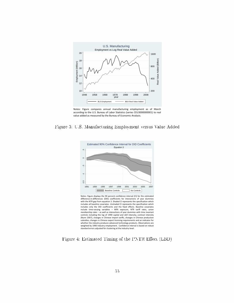
������ ���� �� ����� ����� ��������� � ���� ��� �� �� �����
�������� �� ��� ���� ���� �� ����� ���������� ������� ��� !!!!!!!!"# �� ����
$��� ����� �� ������ �� ��� ���� �� ����� �� %��������
200
400
800
1600
Rea
l Val
ue A
dded
(B
illio
n)
10
12
14
16
18
20
Em
ploy
men
t (M
illio
n)
1948 1958 1968 1978 1988 1998 2008year
BLS Employment BEA Real Value Added
Employment vs Log Real Value AddedU.S. Manufacturing
Figure 3: U.S. Manufacturing Employment versus Value Added
-1.5
-1-.
50
.5
1991 1993 1995 1997 1999 2001 2003 2005 2007
Baseline Controls No Controls
Equation 3Estimated 90% Confidence Interval for DID Coefficients
������ ���� ��� ���� ��� �� ������ ���������� �������� ���� ��� ��� ���������
������������������������� ����� ������������ ��� ������������ �� ���� ������
���� ��� � ! � ���� �"����� #$ %����� �� �� ������� ��� � ����������� �����
������� ��� &������� ����������$ '������� �� �� ������� ��� � ����������� �����
������� ���� ��� ��� ������������ ��� ��� ��(�� �������$ )������� ����������
������ ����������� �����&��� * +�, �( ����- � ! ������ �����- ����
���&����� ����� * �� ���� �� ������������ �� ���� ������ ���� ���� ���������
�������� ������� ��� �� �� .��� �� ���� ��� �/��� ���������- �������� ���������
���� 0��1�- ������ �� ������� �� ��� �������- ������ �� ������� ��������
�&������- ������ �� ������� �( ��� �������� ��"�������� ��� �� ��������� ���
������� ��� ������� ������ �������� ��������� ������$ 2&���������� ���
������� &� .��� ������� �� �������$ ���������� �������� �� &���� �� ��&��
�������� ������ ��3���� ��� �������� �� ��� ������� �����$
Figure 4: Estimated Timing of the PNTR E�ect (LBD)
55


