

The University of Manchester Research
The Trend is Your Friend: Time-Series MomentumStrategies Across Equity and Commodity MarketsDOI:10.1093/rof/rfw048
Document VersionAccepted author manuscript
Link to publication record in Manchester Research Explorer
Citation for published version (APA):Georgopoulou, A., & Wang, G. (2016). The Trend is Your Friend: Time-Series Momentum Strategies Across Equityand Commodity Markets. Review of Finance, 21(4), 1557–1592. https://doi.org/10.1093/rof/rfw048
Published in:Review of Finance
Citing this paperPlease note that where the full-text provided on Manchester Research Explorer is the Author Accepted Manuscriptor Proof version this may differ from the final Published version. If citing, it is advised that you check and use thepublisher's definitive version.
General rightsCopyright and moral rights for the publications made accessible in the Research Explorer are retained by theauthors and/or other copyright owners and it is a condition of accessing publications that users recognise andabide by the legal requirements associated with these rights.
Takedown policyIf you believe that this document breaches copyright please refer to the University of Manchester’s TakedownProcedures [http://man.ac.uk/04Y6Bo] or contact [email protected] providingrelevant details, so we can investigate your claim.
Download date:13. Mar. 2022

The Trend is Your Friend: Time-series Momentum Strategies across Equity and Commodity Markets
Athina Georgopoulou, Jiaguo (George) Wang*
This revision: May 2016
Forthcoming at the Review of Finance
Abstract
This paper documents a significant time-series momentum effect that is consistent and robust
across all examined conventional asset classes from 1969 to 2015. We find that the duration
and magnitude of time-series momentum is different in developed and emerging markets, but
this is no longer the case when controlling for the currency component. We further
demonstrate that time-series momentum captures a significant proportion of international
mutual fund performance, but this is predominantly with respect to its long aspect. Finally,
the market interventions by central banks in recent years have distorted correlations across
assets; this challenges the performance of such portfolios.
JEL classification: G12, G13, G15, G23, G11
Keywords: Return Predictability, Momentum, International Mutual Funds, Market Efficiency,
International Financial Markets
* Georgopoulou is with SEI Investments London Office and Wang is with Manchester Business School. Contact email [email protected]. We would like to thank Bernard Dumas (the Editor), two anonymous referees, Mike Bowe, Ian Garett and Spencer Martin for helpful comments. Part of this version was completed while George was a visiting research professor at NYU Stern, and he would like to thank the host Stephen Brown and the people there for their hospitality and helpful comments.
“Over time, value is roughly the way the market prices stocks, but over the short term, which sometimes can be as long as two or three years, there
are periods when it doesn’t work. And that is a very good thing.”
― Jack D. Schwager
1. Introduction The momentum anomaly can be encountered in two dimensions: cross-sectional and
time-series. According to the traditional and well-documented idea of cross-sectional
momentum, instruments that outperform their peers in a three- to twelve-month period tend to
do so also over the next year.2 A newer version of the momentum anomaly refers to time-
series momentum, which focuses on an instrument’s absolute performance. In particular,
according to the time-series momentum perspective, an asset’s past performance predicts its
future performance, emphasizing the crucial role of autocorrelation in returns. Moskowitz,
Ooi, and Pedersen (2012) are the first to provide evidence of the existence of time-series
momentum with respect to futures markets. They find that excess return during the preceding
12-month period of a futures contract is a positive predictor of its future return during the
next year and that a diversified portfolio that buys instruments that have been in an uptrend
and sells those that have been in a downtrend delivers substantial abnormal returns.3
Recent studies on time-series momentum have focused primarily on futures markets
and managed futures funds (e.g., Baltas and Kosowski, 2013; Moskowitz et al., 2012). Given
that more than 9.5 trillion U.S. dollars in assets are estimated to have been benchmarked to
global equity (i.e., MSCI indexes) and commodity indexes (i.e., S&P GSCI) by the end of
2014 and that there is an increasing number of international mutual funds and exchange
traded funds (ETFs), academic research has devoted surprisingly little attention to trend
following and time-series momentum effects among conventional asset classes.4
Our paper makes three major contributions to the existing literature. First, this study is
among the first to examine the relevance and effectiveness of time-series momentum in
2 Extensive studies have provided evidence of the cross-sectional momentum profitability for several decades (e.g., Jegadeesh and Titman, 1993; Asness, 1994; Grundy and Martin, 2001; Griffin, Ji, and Martin, 2003; Yao 2012); and across various asset classes and countries (e.g., Asness, Liew, and Stevens, 1997; Rouwenhorst, 1998; Moskowitz and Grinblatt, 1999; Bhojraj and Swaminathan, 2006; Erb and Harvey, 2006; Gorton, Hayashi, and Rouwenhorst, 2008; Garleanu and Pedersen, 2009; DeMiguel, Nogales, and Uppal, 2010; and Asness, Moskowitz and Pedersen, 2013). 3 Baltas and Kosowski (2013) confirm the profitability of time-series momentum strategies in global futures markets, and they further show that time-series momentum strategies explain a significant part of hedge fund returns. Menkhoff et al. (2012), however, find that cross-sectional momentum outperforms time-series in the currency market. 4 MSCI stands for Morgan Stanley Capital Indexes. GSCI stands for Goldman Sachs Commodity Indexes. The actual figures are available at www.msci.com/indexes.
2

conventional asset classes. 5 In particular, we find the nature of time-series momentum
strategies is different in developed and emerging markets. For instance, emerging markets
experience much higher time-series momentum returns compared to developed markets. The
time-series momentum phenomenon, however, is of a shorter duration in emerging markets,
and the profitability of such strategies starts to dissipate much more quickly than in
developed markets. To shed some light on this fundamental difference, we apply time-series
strategies in developed and emerging markets by examining both their USD and local
returns.6 Remarkably, we find that the profits in emerging markets are no longer short-term in
nature once we control for the currency component. Instead, the lasting effect of time-series
momentum appears overall very similar for both markets. We further investigate the return
continuation pattern in the currency component of the developed and emerging market equity
indices, and we find the magnitude of this pattern is larger for emerging markets than for
developed ones, especially in the short term.7 Therefore, the difference in the currency return
continuation patterns largely explains the different time-series momentum profitability for
emerging and developed markets.
A second major contribution of our work is to directly link time-series momentum to
the performance of international mutual funds. We accordingly provide a new benchmark to
evaluate international fund performance. Over the years, trend-following strategies have
become one of the most important investment strategies in the hedge fund universe. For
instance, Moskowitz et al. (2012), Baltas and Kosowski (2013), and Hurst, Ooi, and Pedersen
(2014) document that a substantial part of the hedge fund industry, such as managed futures
funds and commodity trading advisors (CTAs), follows time-series momentum strategies. We
extend this line of research by examining whether particular strategies can be associated with
other types of institutional investors, i.e., international mutual funds, which can be
characterized as more traditional and risk-averse, or whether they strictly concern the hedge
fund industry.
We find that the time-series momentum trading strategy explains a significant
proportion of international mutual fund performance, but mainly with respect to its long-only
5 We thank an anonymous referee suggesting that the differences between cash and future market momentum could be due to the role of the futures roll return and the difference between using cash equity indices and futures. We do not further illustrate the difference between future and current market as it is not the main focus of the current paper. Our main interest is on traditional asset classes rather than futures market which have been comprehensively investigated in recent literature (e.g. Moskowitz et al., 2012; Baltas and Kosowski, 2013). 6 We thank an anonymous referee for motivating relevant tests. Here our findings are also consistent with the currency momentum findings in Menkhoff et al. (2012). 7 Our findings are consistent with the currency momentum strategies proposed by Menkhoff et al. (2012). We do not further investigate currency momentum since it is not the focus of this paper.
3
aspect. 8 Specifically, international mutual funds have proven to be long-only time-series
momentum investors, implying that they tend to buy instruments that have been in an
uptrend, but they do not sell those that have been in a downtrend. Indeed, a long-only
portfolio that invests in instruments that have been performing well or that are in risk-free
assets almost entirely captures mutual fund behavior. Therefore, it is likely that mutual funds
will show an investment preference for long-only trend-following strategies. These findings
are consistent and robust across all samples of asset classes and mutual funds examined.
Moreover, they complement existing literature on cross-sectional momentum (e.g., Grinblatt,
Titman, Wermers, 1995; Breloer, Scholz and Wilkens, 2014), where there is evidence that
mutual funds have a tendency to buy winners but do not systematically sell losers.
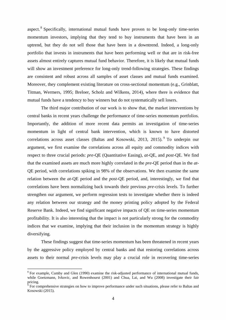
The third major contribution of our work is to show that, the market interventions by
central banks in recent years challenge the performance of time-series momentum portfolios.
Importantly, the addition of more recent data permits an investigation of time-series
momentum in light of central bank intervention, which is known to have distorted
correlations across asset classes (Baltas and Kosowski, 2013, 2015). 9 To underpin our
argument, we first examine the correlations across all equity and commodity indices with
respect to three crucial periods: pre-QE (Quantitative Easing), at-QE, and post-QE. We find
that the examined assets are much more highly correlated in the pre-QE period than in the at-
QE period, with correlations spiking in 98% of the observations. We then examine the same
relation between the at-QE period and the post-QE period, and, interestingly, we find that
correlations have been normalizing back towards their previous pre-crisis levels. To further
strengthen our argument, we perform regression tests to investigate whether there is indeed
any relation between our strategy and the money printing policy adopted by the Federal
Reserve Bank. Indeed, we find significant negative impacts of QE on time-series momentum
profitability. It is also interesting that the impact is not particularly strong for the commodity
indices that we examine, implying that their inclusion in the momentum strategy is highly
diversifying.
These findings suggest that time-series momentum has been threatened in recent years
by the aggressive policy employed by central banks and that restoring correlations across
assets to their normal pre-crisis levels may play a crucial role in recovering time-series
8 For example, Cumby and Glen (1990) examine the risk-adjusted performance of international mutual funds, while Goetzmann, Ivkovic, and Rowenhourst (2001) and Chua, Lai, and Wu (2008) investigate their fair pricing. 9 For comprehensive strategies on how to improve performance under such situations, please refer to Baltas and Kosowski (2015).
4
momentum attractiveness. It would be also interesting to examine the behavior of time-series
momentum as we move further ahead from the end of the QE era. Another important paper in
the field is that of Baltas and Kosowski (2015), who demonstrate that weighting schemes
which incorporate correlation could improve the net of transaction costs performance during
the post global financial crisis period. The effect of monetary policy on such a diverse set of
assets, such as global equity and commodity assets, calls for comprehensive theoretical and
empirical research, including a clearly spelled out economic transmission mechanism.10
Moreover, we find that a diversified long-short time-series momentum portfolio
realizes its largest profits in extreme market conditions.11 Specifically, we find that time-
series momentum serves as a hedging strategy in all conventional asset classes examined and
that its payoffs resemble those of an option straddle, which is consistent with Moskowitz et
al. (2012). Time-series momentum experiences its highest gains during extreme markets. To
enhance our understanding further, we also examine a less volatile short-term time-series
momentum strategy and find that not only does it perform better throughout the period, but it
also serves as a better hedging tool than the longer-term one.12 These results suggest that the
time-series momentum profitability is more likely to be a function of its look-back period and
the established trend at that point.
The rest of this paper is organized as follows. Section 2 reviews the related literature.
Section 3 describes the dataset and the methodology used for constructing momentum
strategies. Section 4 presents the results of time-series momentum trading strategies, while
Section 5 presents evidence that international mutual fund performance is closely related to
time-series momentum trading strategies. Section 6 investigates time-series momentum
profitability during extreme market conditions and the role of central banks. Section 7
presents our conclusions.
2. Related Literature
2.1 Evidence for Time-Series Momentum
In 2012, Moskowitz, Ooi, and Pedersen provided alternative evidence to the
momentum phenomenon, focusing on what they called time-series momentum. They describe
time-series momentum as an asset-pricing anomaly in which an instrument’s past return is
10 We thank an anonymous referee for suggesting this point. 11 We thank an anonymous referee for suggesting this point. The exploration of the differences in the magnitude of momentum crashes with respect to the two momentum strategies sheds more light on our findings. 12 For brevity, the result for shorter term momentum strategies (e.g. 3-1 strategy) is briefly described in footnote 19. Detailed results are available upon request.
5

positively correlated with its future return over a period of 1 to 12 months. This suggests that
one could generate higher returns simply by using long instruments with recent positive
returns and going short for those with recent negative returns. Moskowitz et al. (2012)
examine this trend-following phenomenon for 58 futures and forward contracts from various
asset classes and find that it persists in each of the contracts they study. They also note that
returns generated by time-series momentum strategies partially reverse over longer horizons,
supporting behavioral explanations of initial under-reaction and delayed over-reaction.
Moskowitz et al. (2012) note that time-series momentum is related to but distinct
from the classic cross-sectional momentum of Jegadeesh and Titman (1993). In order to
investigate this, they decompose returns into time-series and cross-sectional momentum
strategies, and they find that lead-lag effects that contribute to cross-sectional momentum are
not apparent in the case of time-series momentum and that returns of futures contracts have a
positive auto-covariance in common. Based on this finding, they conclude that time-series
momentum can capture some features of cross-sectional momentum.
Interestingly, they also note that superior returns associated with this trend effect are
not due to risk compensation since a time-series momentum strategy performs best during
extreme markets. As a result, their time-series momentum trading strategies exhibit no
relation with risk factors such as HML (the value factor) and SMB (the size factor), but seem
to be partially explained by momentum factors, supporting once again a relationship with
cross-sectional momentum.
Moskowitz et al. (2012) attempt to establish a relationship between the positions of
hedgers and speculators, as well as a relationship between hedge funds returns and time-
series momentum strategies themselves. Notably, they find that speculators and hedgers
engage in time-series momentum strategies, permitting the former to profit at the expense of
the latter. As far as hedge fund investment behavior is concerned, they find that hedge fund
returns can be explained by these trend-following strategies.
2.2 Time-Series Momentum and the Performance of Managed Futures Funds
After the work of Moskowitz et al. (2012) was first released, several studies followed,
and these focused primarily on the source of profitability generated by managed futures funds
and CTAs, which together constitute a substantial part of the hedge fund industry. In
particular, Hurst, Ooi, and Pedersen (2012) observe that trend-following strategies such as
time-series momentum can explain managed futures’ returns. Remarkably, they demonstrate
that, when they control for time-series momentum strategies, excess returns (or alphas)
6

cannot be attributed to other long-only benchmarks. In addition, they also highlight the
relative importance of the horizon of these strategies as well as the asset classes that may be
concerned. They find that most managed futures funds are focused on medium- and long-
term trends, due to lower transaction costs, as well as on fixed income due to its higher
liquidity.
In another paper, Hurst, Ooi and Pedersen (2014) provide evidence for a whole century
of strong performance of time-series momentum strategies, extending the evidence provided
by Moskowitz et al. (2012). Moreover, the authors express their concern about the outlook of
time-series momentum strategies in light of their recent drawdowns. Specifically, they claim
that the current economic environment, with central banks intervening in the market, not only
distorts existing trend patterns, but also leads to increased correlations across futures markets.
Therefore, the diversification benefit previously afforded to momentum strategies has been
substantially reduced since there are fewer independent trend patterns that can be exploited.
However, even in this case, the authors state that managed futures funds could benefit from
emerging equity and currency markets, which are much more liquid than in the past.
Baltas and Kosowski (2013) are also concerned with the relationship between time-
series momentum strategies in futures markets and CTAs, and once again they provide strong
evidence that CTAs follow time-series momentum. In order to better approximate CTA
strategies, they examine higher frequencies such as daily and weekly ones, thereby extending
the approach of Moskowitz et al. (2012). Interestingly, they document that strategies at
different frequencies exhibit low correlations with one another and therefore reflect distinct
continuation phenomena. Additionally, they note that CTAs have been performing poorly
recently, and they consider capacity constraints as a possible reason for this
underperformance. However, their results indicate that there are no significant capacity
constraints on momentum strategies, which is consistent with the view that futures markets
are liquid, but it renders the reason for the underperformance of CTAs unclear.
3. Data and Preliminaries
The present dataset consists of monthly closing prices for 45 equity indices, covering
developed and emerging markets, and 22 commodity indices—in total, 67 different
instruments—from December 1969 through August 2015. All instrument prices are
denominated in U.S. dollars since this study is conducted from a U.S. perspective. In
addition, the dataset includes monthly returns for international, global, and commodity
mutual funds, which are examined to establish a link between time-series momentum and
7

mutual fund behavior.
3.1 International Equity Indices
The dataset for equity indices is obtained from Bloomberg and consists of monthly
closing prices for 45 Morgan Stanley Capital International (MSCI) indices across 23
developed and 22 emerging countries. Price data for equity indices date back to December
1969 or later. The MSCI indices considered are free float-adjusted market capitalization
weighted indices that replicate the equity market performance of developed and emerging
countries (MSCI, 2014). Given that all of the MSCI indices mainly represent large
capitalization and liquid stocks, potential biases due to illiquidity and non-synchronous
trading are eliminated.
3.2 Commodity Indices
The dataset for commodity indices consists of 22 commodity indices, which are
obtained from Bloomberg and date back to December 1969. The dataset is based on the
Standard and Poor’s Goldman Sachs Commodity Index (S&P GSCI), which is designed to
track an unleveraged and long-only investment in commodity futures and is diversified across
individual commodity components (S&P GSCI, 2014). The commodity indices are weighted
to account for economic significance and market liquidity. It is important to highlight that
when it comes to returns, excess return indices are considered instead of total returns indices
to take into account the effects of contango and normal backwardation in these markets.
[Insert Table I here]
Table I presents some descriptive statistics for all instruments considered in the
present dataset with regard to the beginning of the time-series of data: annualized mean,
annualized volatility, skewness, and kurtosis. Looking at these quantities of interest, one can
observe that there is a substantial variation in the annualized mean returns across assets, with
equity indices generating primarily positive returns, while many commodity indices yield
negative returns over the sample period.
As far as the annualized volatilities are concerned, many extreme observations that are
even higher than 100% can be noted, especially in emerging and commodity markets. In
contrast to Moskowitz et al. (2012) and Baltas and Kosowski (2013), however, volatilities
across asset classes and instruments are more homogeneous and have fewer striking
differences. This is because the present dataset does not include currency or bond markets.
Finally, the dataset demonstrates reasonable levels of skewness and kurtosis.
8

3.3 Time-Series Return Predictability
Given that time-series momentum strategies are considered trend-following strategies,
it is of great importance to detect price continuation patterns before implementing them. Price
continuation patterns would signify return predictability, and that would further suggest that a
time-series momentum strategy can generate substantial profits. For this purpose and in a
fashion similar to that of Moskowitz et al. (2012), the price continuation is examined across
all instruments combined, by regressing the excess return 13 , scaled by volatility, for
instrument j in month t on its own return lagged h months. Thus, the pooled panel linear
regression can be estimated as follows:
𝒙𝒙 = 𝒓𝒓𝒕𝒕𝒋𝒋
𝝈𝝈𝒕𝒕𝒋𝒋 = 𝒂𝒂 + 𝜷𝜷𝒉𝒉
𝒓𝒓𝒕𝒕−𝒉𝒉𝒋𝒋
𝝈𝝈𝒕𝒕−𝒉𝒉𝒋𝒋 + 𝜺𝜺𝒕𝒕 (1)
where 𝑟𝑟𝑡𝑡𝑗𝑗 and 𝜎𝜎𝑡𝑡
𝑗𝑗 are the excess return and realized volatility of instrument j in month t, and
𝜎𝜎𝑡𝑡−ℎ𝑗𝑗 𝑟𝑟𝑡𝑡−ℎ
𝑗𝑗 are the excess return and realized volatility of instrument j in month t lagged h
months.
The regression defined in Equation (1) is a pooled panel regression in which all
instruments (67 in total) and dates are combined to generate the beta coefficients. The
number of lags for each instrument extends to 60 months (h = 1, 2,…, 60), and thus 60
regressions are estimated. In this regression, the quantity of interest is the t-statistic, where a
significant t-statistic indicates the existence of time-series return predictability. Specifically, a
positive t-statistic signifies return continuation, whereas a negative t-statistic signifies a
reversal.
[Insert Figure 1 here]
Figure 1 presents the t-statistics of the beta coefficients with regard to the pooled
panel regression for lags h = 1, 2,…, 60. When asset classes are examined at an aggregate
level (Panel A), it can be noted that the t-statistics in all of the first 12 lagged months are
positive and significant. Over longer horizons (13 to 60 lags), the t-statistics deliver lower
positive values and, in some cases, significantly negative values. These results indicate the
existence of a return continuation for the first year that subsequently gives rise to weaker
reversals. As a result, the hypothesis for time-series return predictability can be confirmed.
This implies that past returns are able to predict future returns and that trend-following
patterns are thereby created.
These findings are consistent with those documented by Moskowitz et al. (2012) and
13 Data on the three-month Treasury bill are obtained from Bloomberg and used to represent the risk-free rate.
9

Baltas and Kosowski (2013) with respect to return continuations and reversals in futures
markets. Nonetheless, in the present case, the return continuation seems to be more persistent
given some positive spikes at lags greater than 12. Apart from that, reversals in returns
generate weaker signals than those reported by Moskowitz et al. (2012). Baltas and Kosowski
(2013) are also unable to show strong reversals over longer horizons, arguing that this result
is due to the use of a larger sample in both time-series and cross-sectional dimensions. This
rationale can also be inferred from our present study, where the dataset starts in 1969 and
consists of 67 instruments.
As far as asset classes are concerned, the return predictability seems to be slightly
stronger in the case of equity versus commodity indices. In the case of equity indices, 11 out
of 12 lags are positive and significant, whereas only 7 out of 12 lags are positive and
significant for commodity indices. Also, the return continuation tends to be more persistent
and decays to a smaller extent for equity indices. Hence, it is expected that time-series
momentum strategies will be more profitable for equity than for commodity indices. We also
observe more pervasive continuation signals for developed than for emerging equity indices,
indicating higher time-series profitability for the former.
3.4 International Equity and Commodity Funds
Mutual fund data are obtained from the Morningstar Direct database and cover the
period from December 1968 through August 2015. The sample contains all international
equity funds, along with commodity funds that exist at any time during the period of 1968 to
2015. The data used for international equity funds begin in December 1968, while that for
commodity funds begin in April 1997. All the relevant values are reported in U.S. dollars and
the oldest share class data is retained in the sample. Our final sample includes 1,177
international equity fund-entities and 106 commodity fund-entities, comprising 154,259
monthly fund data-points. The number of international equity funds increases steadily starting
from five funds in 1968 and reaching 1,084 funds in 2015. Commodity investments seem to
be less popular, with commodity fund data existing only from 1997 counting only to one at
that time and growing to 70 by 2015.
[Insert Table II here]
Sample descriptive statistics are presented in Table II. When looking at the total net
assets across the various fund categories, we conclude that the highest interest is concentrated
in emerging markets since the value of total net assets there is the largest compared to
commodity and developed funds. Nonetheless, we recognize that many smaller cap funds can
10

be found in developed markets so that our sample might be biased. In unreported results,
though, and after excluding small caps from our sample in developed markets, the mean and
median of total net assets increase to 911.03 and 925.96 million, respectively, and these
figures are still significantly lower than those observed in funds investing in emerging
markets. After controlling for the small cap bias, variability of returns also decreases to levels
similar to those in emerging markets. Turnover for commodity funds is much higher
compared to developed and emerging market equity funds, while their returns are modest on
a relative basis but have higher variability, followed by emerging and then developed
international equity funds.
[Insert Figure 2 here]
In Figure 2 in panels A and B, we present the geographical distribution for
international equity funds and the holdings distribution for commodity funds, respectively.
We base our classification on the Morningstar Category, Investment Area and Primary
Prospectus Benchmark for the equity funds and on the Morningstar Category and GIFS for
the commodity funds. For the international equity funds, we observe that almost 67% of them
invest on a global and well-diversified basis without showing an investment interest in a
specific region. The majority of these funds are assigned to a broad benchmark, such as the
MSCI World Index, MSCI ACWI Index, and MSCI EAFE, among others. Many funds show
a particular interest in individual regions or countries, among which 27% of the whole sample
represent emerging market countries or regions, whereas only 6% target individual developed
countries or areas. As far as the commodity fund holdings are concerned, 81% of them are
well-diversified and are investing in a broad basket of commodities throughout the sample
period. Some show a preference for a specific sub-asset class, which seems to concentrate in
precious metals followed by agriculture and energy.
4. Trading Strategies and Empirical Analysis
4.1 Time-Series Momentum Strategies
In Section 3.3, the positive correlation between past returns and future returns
suggests the existence of trend-following patterns. Therefore, it is reasonable to construct
time-series momentum strategies that take advantage of these patterns and to evaluate their
profitability.
Before analyzing the methodology for constructing time-series momentum strategies,
it is of great importance to highlight that these strategies can be constructed based on
11
different time horizons. Thus, it is essential to define the periods involved in constructing
time-series momentum strategies: the look-back or formation period and the holding period.
The look-back period J refers to the number of lagged months in which returns are examined
to form the momentum portfolio, while the holding period K refers to the number of months
that the momentum portfolio is held after it is formed. K and J can vary through time,
allowing for different combinations of look-back and holding periods. Therefore, a 12-1
strategy, where 12 indicates the look-back period J and 1 indicates the holding period K,
refers to a portfolio that is constructed based on the instrument returns over the previous 12
months and is held for one month after its formation.
As in Moskowitz et al. (2012), Baltas and Kosowski (2013), and Hurst et al. (2012), a
time-series momentum strategy takes a long (short) position for a single instrument when the
sign of its cumulative return over a particular look-back period is positive (negative). The
trading sign takes the value 1 if the cumulative return of the asset over the look-back period J
is positive and the value -1 if otherwise. The time-series momentum return of each instrument
is calculated based on the trading sign and the return over the holding period. Moreover,
similarly to Jegadeesh and Titman (1993), one month is skipped between the formation and
holding periods to avoid some of the bid-ask spread, price pressure, and lagged reaction
effects (Jegadeesh, 1990; Lehmann, 1990). Subsequently, time-series momentum returns are
aggregated to form the momentum portfolios as follows:
𝑷𝑷𝑱𝑱𝑲𝑲 = 𝟏𝟏𝑵𝑵𝒕𝒕∑ 𝒔𝒔𝒊𝒊𝒊𝒊𝒊𝒊𝒂𝒂𝒊𝒊𝒋𝒋𝑵𝑵𝒕𝒕𝒊𝒊=𝟏𝟏 (𝒄𝒄𝒄𝒄𝒄𝒄𝒓𝒓𝒕𝒕−𝑱𝑱,𝒕𝒕
𝒋𝒋 )𝒓𝒓𝒕𝒕,𝒕𝒕+𝑲𝑲𝒋𝒋 (2)
where 𝑁𝑁𝑡𝑡 indicates the number of available instruments at time, t, 𝑃𝑃𝐽𝐽𝐾𝐾 is the return on the
time-series momentum portfolio with a look-back period of J months and holding period of K
months, 𝑠𝑠𝑠𝑠𝑠𝑠𝑠𝑠𝑠𝑠𝑠𝑠𝑗𝑗 takes the value 1 (-1) if the cumulative return 𝑐𝑐𝑐𝑐𝑐𝑐𝑟𝑟𝑡𝑡−𝐽𝐽,𝑡𝑡𝑗𝑗 in month t for
instrument j over the past J months is positive (negative), and 𝑟𝑟𝑡𝑡,𝑡𝑡+𝐾𝐾𝑗𝑗 is the return with respect
to a holding period of K months.
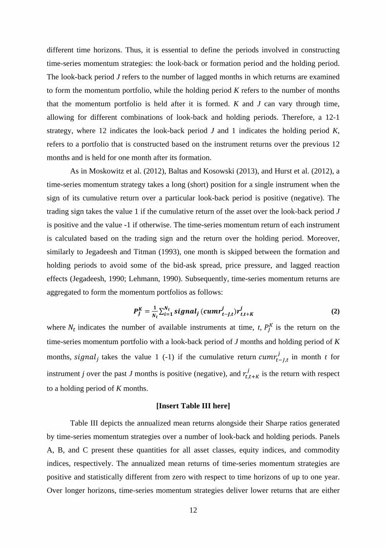
[Insert Table III here]
Table III depicts the annualized mean returns alongside their Sharpe ratios generated
by time-series momentum strategies over a number of look-back and holding periods. Panels
A, B, and C present these quantities for all asset classes, equity indices, and commodity
indices, respectively. The annualized mean returns of time-series momentum strategies are
positive and statistically different from zero with respect to time horizons of up to one year.
Over longer horizons, time-series momentum strategies deliver lower returns that are either
12

not significant or negative (for commodity indices, Panel C). These findings confirm the
price continuation patterns detected in the previous section and the results documented in the
time-series momentum literature. It can therefore be concluded that, apart from the case of
futures markets, time-series momentum can successfully be applied to a more traditional
range of instruments, such as equity and commodity indices. Moreover, the particular
strategies seem to yield a respectable 0.77 Sharpe ratio when applied for up to one year.
Time-series momentum strategies can also successfully be applied to individual stocks.
Further investigation of individual stocks, however, is beyond the scope of this study.
Taking a closer look at panels B and C, where each asset class is examined separately,
one can observe that time-series momentum profitability is slightly more pronounced across
equity indices than commodity indices. More precisely, time-series momentum delivers
annualized returns in the range of 2% to 15% with regard to equity markets, and 2% to 10%
with regard to commodity markets. The higher momentum profitability of equity indices is
further supported by noticing their respective Sharpe ratios, which seem superior in equity
markets.
These findings confirm the predictability patterns observed in the previous section,
where return continuations proved to be stronger for equity indices. Surprisingly, reversal
patterns in time-series momentum returns are observed only for commodity indices, while
with equity indices, only weaker positive returns are noted. This might also be the reason
why, when the aggregate strategy is examined, similar behavior can be observed. Once again,
these findings are in line with those reported by Baltas and Kosowski (2013), who could not
find strong reversals over longer horizons. Adopting the arguments of Baltas and Kosowski,
this paper therefore suggests that the use of a larger sample both for time-series and cross-
sectional analysis provides one reason why strong reversals are not noted.
4.2 Time-Series Momentum Strategies across Developed and Emerging Markets
In order to further investigate time-series momentum across equity markets, equity
indices are distinguished for developed and emerging markets. This allows examining
whether time-series momentum patterns are similar in these two different types of market.
[Insert Table IV here]
Table IV provides evidence of the different behavior of time-series momentum with
respect to developed and emerging markets. In particular, it can be noted that emerging
markets experience much higher time-series momentum returns compared to developed
13

markets. However, the time-series momentum phenomenon is of a shorter duration in the
case of emerging markets. Indeed, the profitability of these strategies starts to dissipate much
more quickly for emerging markets. To shed some light on this fundamental difference, we
perform the same analysis, but this time we use local currency terms rather than the U.S.
dollar.
An initial observation we make is that returns and Sharpe ratios appear enhanced in
local terms (Part A of Table IV) compared to U.S. dollar terms (Part B of Table IV) in regard
to both developed and emerging markets. For developed markets, returns are on average
augmented by 34bps, but the biggest difference is noted for emerging markets whose returns
are improved by 180bps. We also observe, that profits to time-series momentum in emerging
markets are no longer short-term in nature once we control for the currency component.
Instead, the lasting effect of time-series momentum appears very similar for both markets.
These results make us consider that there might be differences in the return continuation
patterns for developed and emerging currency returns. Hence, we isolate the currency return,
based on the following equation:
𝑹𝑹𝒄𝒄𝒄𝒄𝒓𝒓𝒓𝒓𝒊𝒊,𝒕𝒕 = 𝑹𝑹𝑹𝑹𝑹𝑹𝑹𝑹𝒊𝒊,𝒕𝒕 − 𝑹𝑹𝒊𝒊𝑹𝑹𝒄𝒄𝒂𝒂𝒊𝒊𝒊𝒊,𝒕𝒕 (3)
where 𝑅𝑅𝑅𝑅𝑅𝑅𝑅𝑅𝑖𝑖,𝑡𝑡 is the return of index i in month t in U.S. dollar terms and 𝑅𝑅𝑠𝑠𝑅𝑅𝑐𝑐𝑠𝑠𝑠𝑠𝑖𝑖,𝑡𝑡 is the
return of index i in month t in local terms.
After extracting the currency component for each of the country indices, we examine
its return continuation pattern by regressing the currency return for index i in month t on its
own return lagged h months, similar to the previous pooled panel regressions for the price
continuation patterns. Thus, the pooled panel regression can be specified as follows:
𝑹𝑹𝒄𝒄𝒄𝒄𝒓𝒓𝒓𝒓𝒊𝒊,𝒕𝒕 = 𝜶𝜶 + 𝜷𝜷𝒉𝒉𝑹𝑹𝒄𝒄𝒄𝒄𝒓𝒓𝒓𝒓𝒊𝒊,𝒕𝒕−𝒉𝒉 + 𝜺𝜺𝒕𝒕 (4)
where 𝑅𝑅𝑐𝑐𝑐𝑐𝑟𝑟𝑟𝑟𝑖𝑖,𝑡𝑡 is the currency return of index i in month t and 𝑅𝑅𝑐𝑐𝑐𝑐𝑟𝑟𝑟𝑟𝑖𝑖,𝑡𝑡−ℎ is the currency
return of index i in month t lagged h months.
The regression defined in the above equation is a pooled panel regression in which all
equity developed indices (23 in total) or emerging indices (22 in total) and dates are
combined to generate the beta coefficients. The number of lags for each instrument extends to
60 months (h = 1, 2,…, 60), and thus 60 regressions are estimated.
[Insert Figure 3 here]
14

As expected, in Figure 3, we note that there is indeed return continuation in the
currency component of the developed and emerging market equity indices.14 Similar to the
price continuation patterns, there is a time-series continuation pattern for currencies which
reverses or dissipates after the 12th lag. It is interesting to see that the magnitude of this
pattern is larger for emerging markets than for developed ones, especially with respect to the
first lag, but also thereafter in some cases. We also see a slightly different pattern for
emerging markets which exhibit significant and negative reversals for lags smaller than 12
(i.e., lags 7 and 11). These findings largely help to explain the different time-series
momentum profitability for emerging and developed markets. We also show with these
results that the higher short-term momentum profits can be attributed to higher time-series
currency return predictability.
4.3 Evaluating Time-Series Momentum Strategies
Following the significant time-series momentum profitability observed above, this
section aims to further investigate the abnormal performance of time-series momentum by
estimating some standard asset pricing models. Specifically, the single diversified-across-
assets 12-1 time-series momentum strategy is investigated since, as already mentioned, it
serves as a benchmark in the existing literature.
To better investigate the performance of time-series momentum strategies, we regress
time-series momentum returns on a number of factors. This allows for better evaluation of the
drivers of time-series momentum profitability. Attention is drawn to the single diversified15
12-1 time-series momentum strategy, which serves as the benchmark in the momentum
literature and refers to a strategy with a look-back period of 12 months and a holding period
of 1 month. The specified model can be estimated as follows:
𝑻𝑻𝑹𝑹𝑻𝑻𝑻𝑻𝑻𝑻𝒕𝒕,𝒊𝒊(𝟏𝟏𝟏𝟏,𝟏𝟏) = 𝜶𝜶 + 𝜷𝜷𝟏𝟏𝑻𝑻𝑹𝑹𝑴𝑴𝑴𝑴𝒕𝒕 + 𝜷𝜷𝟏𝟏𝑮𝑮𝑹𝑹𝑴𝑴𝑴𝑴𝒕𝒕 + 𝜷𝜷𝟑𝟑𝑹𝑹𝑻𝑻𝑺𝑺𝒕𝒕 + 𝜷𝜷𝟒𝟒𝑯𝑯𝑻𝑻𝑯𝑯𝒕𝒕 + 𝜷𝜷𝟓𝟓𝑹𝑹𝑻𝑻𝑹𝑹𝒕𝒕 + 𝜺𝜺𝒕𝒕 (5)
where 𝑇𝑇𝑅𝑅𝑇𝑇𝑇𝑇𝑇𝑇𝑖𝑖,𝑡𝑡(12,1)is the equally-weighted average return across instruments of the single
diversified time-series momentum strategy in month t for asset class i, with a look-back
period of 12 months and a holding period of 1 month, 𝑇𝑇𝑅𝑅𝑀𝑀𝑀𝑀𝑡𝑡 is the return of the MSCI World
Index in month t, 𝐺𝐺𝑅𝑅𝑀𝑀𝑀𝑀𝑡𝑡 is the return of the S&P GSCI in month t, and the SMB, HML, and
UMD regressors are Fama-French factors representing size, value, and momentum across
U.S. stocks, respectively.
14 This is consistent with the currency momentum findings documented by Menkhoff et al. (2012). 15 In this study, diversified returns refers to equally-weighted average returns across all instruments.
15
Given that the present dataset concerns instruments from different asset classes and
markets, the strategy is further regressed on alternative factors, including momentum
everywhere factors from Asness et al. (2013), and, as such, it better resembles the present
dataset. These factors replace the Fama-French factors, which are limited to U.S. stocks.
However, since the present dataset excludes foreign exchange markets as well as bond
markets, the momentum everywhere factors are adjusted to reflect this change and to
represent the dataset as closely as possible. Thus, the specified model can be written as:
𝑻𝑻𝑹𝑹𝑻𝑻𝑻𝑻𝑻𝑻𝒕𝒕,𝒊𝒊(𝟏𝟏𝟏𝟏,𝟏𝟏) = 𝜶𝜶 + 𝜷𝜷𝟏𝟏𝑻𝑻𝑹𝑹𝑴𝑴𝑴𝑴𝒕𝒕 + 𝜷𝜷𝟏𝟏𝑮𝑮𝑹𝑹𝑴𝑴𝑴𝑴𝒕𝒕 + 𝜷𝜷𝟑𝟑𝑽𝑽𝑽𝑽𝑯𝑯𝒕𝒕 + 𝜷𝜷𝟒𝟒𝑻𝑻𝑻𝑻𝑻𝑻𝒕𝒕 + 𝜺𝜺𝒕𝒕 16 (6)
where the first two regressors remain the same, while VAL and MOM represent value and
momentum, respectively, and replace the Fama-French three-factor model.
[Insert Table V here]
Table V reports the risk-adjusted performance of the single diversified 12-1 time-
series momentum strategy. It can be observed that the strategy delivers large and significant
alphas in all asset classes, indicating its out-performance relative to the benchmarks included
in the regression.
The diversified time-series momentum strategy exhibits mainly significant beta
coefficients on the cross-sectional momentum factor as proxied by UMD. The significance of
momentum factor UMD is also confirmed with respect to the futures markets explored by
Moskowitz et al. (2012) and Baltas and Kosowski (2013). This finding suggests that some
variation in returns can be explained by cross-sectional momentum. None of the other factors
included can explain the time-series momentum profitability, except for the commodity
benchmark GSCI, which captures some of the time-series momentum profitability with
regard to commodity indices. Nevertheless, the significance observed in the alpha
coefficients implies that GSCI and UMD capture only a part of the time-series momentum
profitability, leaving an important part unexplained.
As a next step, the 12-1 time-series momentum strategy is evaluated with respect to
Equation (6), where the SMB, HML, and UMD factors of Fama and French are replaced with
the momentum everywhere factors constructed by Asness et al. (2013).
[Insert Table VI here]
Table VI reports the risk-adjusted performance of the single diversified 12-1 time-
16 The Variable Inflator Factor (VIF) test is available in the online appendix. Our results indicate that there are no concerns for multi-collinearity across the factors.
16

series momentum strategy with the alternative control variables as specified previously. Once
again, the strategy delivers significant alpha coefficients and loads significantly on the
momentum factor (MOM). However, an important part of the time-series momentum
profitability seems to remain unexplained.17
5. Time-Series Momentum and International Mutual Fund Performance
Following the presented evidence of significant time-series momentum profitability,
this section aims to investigate the relation between mutual fund performance and time-series
momentum. In particular, we examine the nature of investment strategies followed by a
comprehensive list of international mutual funds, and consider whether these can be related to
trend-following strategies such as time-series momentum.
Existing time-series momentum literature focuses primarily on hedge fund behavior,
particularly that of managed futures funds and CTAs, which have been shown to follow time-
series momentum strategies (Baltas and Kosowski, 2013; Moskowitz et al., 2012). As far as
mutual fund behavior is concerned, the existing literature focuses on mutual fund performance
with respect to cross-sectional momentum (Grinblatt et al., 1995; Breloer et al., 2014). The
findings suggest that mutual fund managers tend to be momentum investors who buy past
winners but do not systematically sell past losers. In this study, we seek to investigate mutual
fund performance with regard to time-series momentum strategies. More precisely, the
monthly mutual fund returns net of management expenses and fees is regressed on 12-1 time-
series momentum returns. Given the more traditional and risk-averse nature of mutual funds,
mutual fund returns are also regressed on the returns of a long-only time-series momentum
strategy. The particular strategy used is one of long-only investments in instruments that have
been performing well over the previous 12 months. In cases where there is a sell signal, the
long-only time-series momentum involves investment in the three-month Treasury bill, which
provides the risk-free rate. Hence, mutual fund performance according to these two strategies
can be examined by the following models:
𝑻𝑻𝑴𝑴𝒚𝒚,𝒕𝒕 = 𝜶𝜶 + 𝜷𝜷𝑻𝑻𝑹𝑹𝑻𝑻𝑻𝑻𝑻𝑻𝒊𝒊,𝒕𝒕(𝟏𝟏𝟏𝟏,𝟏𝟏) + 𝜺𝜺𝒕𝒕 (7)
𝑻𝑻𝑴𝑴𝒚𝒚,𝒕𝒕 = 𝜶𝜶 + 𝜷𝜷𝑯𝑯𝑹𝑹𝒊𝒊𝒊𝒊𝒊𝒊,𝒕𝒕(𝟏𝟏𝟏𝟏,𝟏𝟏) + 𝜺𝜺𝒕𝒕 (8)
17 The significance of the momentum coefficients UMD and MOM implies that there exists an important relationship between cross-sectional and time-series momentum. In an unreported appendix, we investigate the relation between time-series and cross-sectional momentum. Results are available upon request.
17
where 𝑇𝑇𝑅𝑅𝑇𝑇𝑇𝑇𝑇𝑇𝑖𝑖,𝑡𝑡(12,1) is the return of the single diversified time-series momentum strategy
described previously, 𝐿𝐿𝑅𝑅𝑠𝑠𝑠𝑠𝑖𝑖,𝑡𝑡(12,1) is the equally-weighted average return across instruments of
the single long-only time-series momentum strategy in month t for asset class i, with a look-
back period of 12 months and a holding period of 1 month, and 𝑇𝑇𝑀𝑀𝑦𝑦,𝑡𝑡 is the equally average
return across mutual funds of type y in month t. Type y refers to commodity, international,
and global mutual funds. Both the standard time-series momentum strategy and the long-only
strategy involve a look-back period of 12 months and a holding period of 1 month.
To better evaluate mutual fund performance, mutual fund returns are regressed on a
specification model that includes certain control variables, as follows:
𝑻𝑻𝑴𝑴𝒚𝒚,𝒕𝒕 = 𝜶𝜶 + 𝜷𝜷𝟏𝟏𝑻𝑻𝑹𝑹𝑻𝑻𝑻𝑻𝑻𝑻𝒊𝒊,𝒕𝒕(𝟏𝟏𝟏𝟏,𝟏𝟏) + 𝜷𝜷𝟏𝟏𝑻𝑻𝑹𝑹𝑴𝑴𝑴𝑴𝒕𝒕 + 𝜷𝜷𝟑𝟑𝑮𝑮𝑹𝑹𝑴𝑴𝑴𝑴𝒕𝒕 + 𝜷𝜷𝟒𝟒𝑽𝑽𝑽𝑽𝑯𝑯 + 𝜷𝜷𝟓𝟓𝑻𝑻𝑻𝑻𝑻𝑻 + 𝜺𝜺𝒕𝒕 (9)
𝑻𝑻𝑴𝑴𝒚𝒚,𝒕𝒕 = 𝜶𝜶 + 𝜷𝜷𝟏𝟏𝑯𝑯𝑹𝑹𝒊𝒊𝒊𝒊𝒊𝒊,𝒕𝒕(𝟏𝟏𝟏𝟏,𝟏𝟏) + 𝜷𝜷𝟏𝟏𝑻𝑻𝑹𝑹𝑴𝑴𝑴𝑴𝒕𝒕 + 𝜷𝜷𝟑𝟑𝑮𝑮𝑹𝑹𝑴𝑴𝑴𝑴𝒕𝒕 + 𝜷𝜷𝟒𝟒𝑽𝑽𝑽𝑽𝑯𝑯 + 𝜷𝜷𝟓𝟓𝑻𝑻𝑻𝑻𝑻𝑻 + 𝜺𝜺𝒕𝒕 (10)
where the first regressors in both equations are the same as those in Equations (7) and (8),
𝑇𝑇𝑅𝑅𝑀𝑀𝑀𝑀𝑡𝑡 is the return of the MSCI World Index at time t, 𝐺𝐺𝑅𝑅𝑀𝑀𝑀𝑀𝑡𝑡 is the return of the S&P GSCI
Index in month t, and 𝑉𝑉𝑉𝑉𝐿𝐿 and 𝑇𝑇𝑇𝑇𝑇𝑇 are the value and momentum everywhere factors from
Asness et al. (2013).
[Insert Table VII here]
Table VII reports the alpha and beta coefficients of the models specified above. It can
be observed in Panel A that international mutual funds exhibit small beta loadings for the 12-1
time-series momentum strategy with and without control variables and the t-statistics are not
statistically different from zero. On the other hand, when we replace the 12-1 strategy with the
long-only strategy, the beta exposures are much stronger both in the univariate and the
multivariate model, and the t-statistics are always significant.18 When we look at the long-
only strategy, the alpha coefficients become insignificant in the univariate model, implying
that these types of fund returns can be largely explained by long-only trend following
strategies. Besides, the R2 improves dramatically for each of the fund types examined. The
above results suggest that international mutual funds have a tendency to focus on recent
winners but do not sell past losers, which is in line with the cross-sectional momentum
findings documented by Grinblatt et al. (1995).
18 In unreported tests, we also replace the 12-1 strategy with the short-only strategy, and find that mutual funds have much smaller exposure on the short side. This is the case both with and without control variables. These results support the argument that international mutual funds do not systematically sell losers or exploit the short-side of time-series momentum due to various reasons and limitations.
18
When we look at the model, including other control variables, the results show that
time-series momentum, both in its long-short and long-only aspects, is unable to entirely
capture mutual fund performance. With respect to equity funds, when we compare the MOM
factor, which captures cross-sectional momentum, with the 12-1 time-series momentum
strategy, it seems that the funds are more related to cross-sectional rather than time-series
momentum strategies. This is not the case for the commodity funds, which exhibit higher
sensitivity to time-series momentum. Given the more exotic nature of commodity funds
compared to traditional equity funds, one might be interested to investigate the relation
between these funds and CTAs. A final observation we make for the equity funds is that the
market factor, along with value strategies, plays a much greater role in explaining
performance, whereas with respect to commodity funds the market is the most determinant
factor.
[Insert Figure 4 here]
We go one step further and examine how the relation between funds and some of the
factors examined previously has evolved over time. It would be of a great interest to perform
a time-series analysis of these relationships, since in this way we would be able to assess the
effects of extreme values and establish common behaviors among the different fund groups.
Figure 4, panels A, B, and C, provide this type of information with regard to developed,
emerging, and commodity funds, respectively. For this purpose we estimate the following
model:
𝑻𝑻𝑴𝑴𝒚𝒚,𝒕𝒕 = 𝜶𝜶 + 𝜷𝜷𝟏𝟏𝑻𝑻𝑹𝑹𝑻𝑻𝑻𝑻𝑻𝑻𝒊𝒊,𝒕𝒕(𝟏𝟏𝟏𝟏,𝟏𝟏) + 𝜷𝜷𝟏𝟏𝑻𝑻𝑹𝑹𝑴𝑴𝑴𝑴𝒊𝒊,𝒕𝒕19 + 𝜷𝜷𝟑𝟑𝑾𝑾𝒊𝒊𝒊𝒊𝒊𝒊𝑾𝑾𝒓𝒓𝒊𝒊,𝒕𝒕
(𝟏𝟏𝟏𝟏,𝟏𝟏) + 𝜷𝜷𝟒𝟒𝑯𝑯𝑹𝑹𝒔𝒔𝑾𝑾𝒓𝒓𝒊𝒊,𝒕𝒕(𝟏𝟏𝟏𝟏,𝟏𝟏) + 𝜷𝜷𝟓𝟓𝑽𝑽𝑽𝑽𝑯𝑯+𝜺𝜺𝒕𝒕 (11)
where the first two and the last regressors have been specified in the previous models,
𝑾𝑾𝒊𝒊𝒊𝒊𝒊𝒊𝑾𝑾𝒓𝒓𝒊𝒊,𝒕𝒕(𝟏𝟏𝟏𝟏,𝟏𝟏) is the equally-weighted average return across instruments of the 12-1 strategy
decomposed into its winner portfolio in month t for asset class i, and 𝑯𝑯𝑹𝑹𝒔𝒔𝑾𝑾𝒓𝒓𝒊𝒊,𝒕𝒕(𝟏𝟏𝟏𝟏,𝟏𝟏) is the
equally- weighted average return across instruments of the 12-1 strategy decomposed into its
loser portfolio in month t for asset class i.
As shown in the above equation, we further decompose the 12-1 TSMOM strategy
into its winner (long positions) and loser (short positions) and regress fund returns on them. In
cases where we notice an extreme market state, such that either the winner or the loser
component does not exist for a particular month, we assign to it a return of zero. The graphs
display the 36-month rolling t-statistics of the beta coefficients of the multivariate regression.
19 GSCI in case of commodity funds
19
The results of the t-statistics indicate distinct herding behavior of the different fund
groups but also some common investment behavior for certain factors. What appears to be the
most significant factor in explaining fund performance is clearly the market itself, measured
as either the equity or commodity market. This is common among all the fund categories we
examine, and the beta coefficients for the market factors are high and almost at all times
significant. A second commonality among all fund types is the ability of the winner’s
portfolio in capturing fund performance, since the factor loading is positive and most of the
times significant. The relation between fund returns and the loser’s portfolio is negative and
statistically different from zero the majority of times, and especially with respect to
commodity and emerging market funds, confirming the findings of Grinblatt et al. (1995) with
respect to losers.
Finally, we notice a fundamental difference in investment philosophy between
commodity and equity funds. It seems that, on average, equity funds seek value as an
investment strategy, whereas commodity funds can sometimes exhibit significantly negative
coefficients on the commodity value factor (VAL). Interestingly, the positive relationship that
the commodity funds exhibit with the winner portfolio over time is much more pronounced
compared to that of equity funds.
6. Market Conditions and the Role of Central Bank Intervention
6.1 Extreme Market Conditions
In this section, the abnormal performance of the aggregate single diversified 12-1
time-series momentum strategy is evaluated with regard to the market portfolio as proxied by
the MSCI World Index.
[Insert Figure 5 here]
Figure 5 shows the growth of an investment of $100 in the aggregate 12-1 time-series
momentum strategy and the MSCI World Index from 1971 to 2015. The figure clearly
highlights the superior performance of time-series momentum relative to the market
throughout the whole sample period. More remarkably, the figure presents the different
responses of time-series momentum and the market during recession periods as defined by
the NBER.20 During these recessions, time-series momentum generated large gains, whereas
the market incurred large losses. Time-series momentum experienced similar large gains
during uptrends of the market.
20 National Bureau of Economic Research. Dates available at: http://www.nber.org/cycles/cyclesmain.html.
20
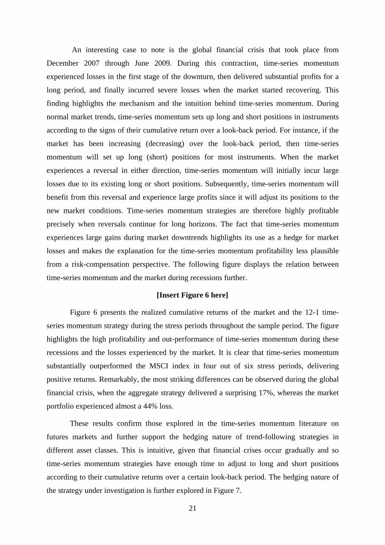
An interesting case to note is the global financial crisis that took place from
December 2007 through June 2009. During this contraction, time-series momentum
experienced losses in the first stage of the downturn, then delivered substantial profits for a
long period, and finally incurred severe losses when the market started recovering. This
finding highlights the mechanism and the intuition behind time-series momentum. During
normal market trends, time-series momentum sets up long and short positions in instruments
according to the signs of their cumulative return over a look-back period. For instance, if the
market has been increasing (decreasing) over the look-back period, then time-series
momentum will set up long (short) positions for most instruments. When the market
experiences a reversal in either direction, time-series momentum will initially incur large
losses due to its existing long or short positions. Subsequently, time-series momentum will
benefit from this reversal and experience large profits since it will adjust its positions to the
new market conditions. Time-series momentum strategies are therefore highly profitable
precisely when reversals continue for long horizons. The fact that time-series momentum
experiences large gains during market downtrends highlights its use as a hedge for market
losses and makes the explanation for the time-series momentum profitability less plausible
from a risk-compensation perspective. The following figure displays the relation between
time-series momentum and the market during recessions further.
[Insert Figure 6 here]
Figure 6 presents the realized cumulative returns of the market and the 12-1 time-
series momentum strategy during the stress periods throughout the sample period. The figure
highlights the high profitability and out-performance of time-series momentum during these
recessions and the losses experienced by the market. It is clear that time-series momentum
substantially outperformed the MSCI index in four out of six stress periods, delivering
positive returns. Remarkably, the most striking differences can be observed during the global
financial crisis, when the aggregate strategy delivered a surprising 17%, whereas the market
portfolio experienced almost a 44% loss.
These results confirm those explored in the time-series momentum literature on
futures markets and further support the hedging nature of trend-following strategies in
different asset classes. This is intuitive, given that financial crises occur gradually and so
time-series momentum strategies have enough time to adjust to long and short positions
according to their cumulative returns over a certain look-back period. The hedging nature of
the strategy under investigation is further explored in Figure 7.
21

[Insert Figure 7 about here]
Figure 7 plots the monthly returns of the 12-1 time-series momentum against those of
the MSCI World Index. The figure highlights the option-like behavior of time-series
momentum. The “smile” indicates that the strategy performs best in extreme up-or-down
market conditions. Fung and Hsieh (2001) demonstrate that trend-following strategies
generate payoffs that are similar to an option straddle on the market, which is also the case in
this figure. Indeed, the payoff shown in Figure 7 resembles that of an option straddle. This
implies that returns on time-series momentum may not be due to compensation for market
crashes, which renders the explanation for time-series momentum profitability even more
puzzling from a risk-adjusted perspective (Moskowitz et al., 2012).21
6.2 The Future of Time-Series Momentum and the Role of Central Banks
In considering the performance of time-series momentum after the end of the global
financial crisis in Figure 2, some would doubt its future and abnormal profitability (e.g.,
Baltas and Kosowski, 2013, 2015). Although the cumulative return on the 12-1 time-series
momentum strategy remains well above the market index, it seems that it entered a
consolidation period for the first time during, and throughout, the sample period. In contrast,
the market seems to have entered a new uptrend over the same period and the time-series
momentum unexpectedly does not deliver substantial profits.
[Insert Table VIII here]
Interestingly, this observation coincides with periods of market intervention by central
banks, which have adopted quantitative easing as a monetary policy, to stimulate the global
economy. We suspect that this aggressive policy has also caused correlations across assets to
be distorted, thereby threatening the trend-following patterns. Το underpin this argument, we
first examine the correlations across all equity and commodity indices with respect to three
crucial periods, as illustrated in Table VIII: pre-QE, at-QE, and post-QE. The first
observation we make is that the examined assets are much more highly correlated in the pre-
21 In unreported tests, we also examine the properties of short term momentum strategies. E.g. we construct a 3-1 time-series momentum strategy similar to the 12-1 but with a look-back period of 3 months. We look at the cumulative performance of the single diversified 3-1 time-series momentum strategy and we make the same observations as with the 12-1.The strategy outperforms the broad market to a great extent over the examined period and also outperforms the 12-1 strategy. It also realizes its largest profits during established and continuous trends of the market, as well as during bad market states. We explore further the superiority of the shorter-term strategy when the market rebounds and when the market crashes during stress periods. We find that the 3-1 strategy outperforms the 12-1 strategy in 8 out of 10 market rebounds and in 6 out of 10 market crashes. Because of that, we also observe that the 3-1 time-series momentum “smile” is more pronounced compared to the 12-1 strategy, rendering the former a better hedge in extreme market states.
22
QE period than in the at-QE period, with correlations spiking in 98% of the observations.22
We then examine the same relation between the at-QE period and the post-QE period, and
remarkably we notice that correlations have been normalizing back towards their previous
pre-crisis levels, which holds true for 66% of the observations. To further strengthen our
argument we perform regression tests to investigate whether there is indeed any relationship
between our strategy and money printing adopted by the Federal Reserve Bank. We examine
this relationship as follows.
𝑻𝑻𝑹𝑹𝑻𝑻𝑻𝑻𝑻𝑻𝒕𝒕,𝒊𝒊(𝟏𝟏𝟏𝟏,𝟏𝟏) = 𝜶𝜶 + 𝜷𝜷𝟏𝟏𝑻𝑻𝑹𝑹𝑴𝑴𝑴𝑴𝒕𝒕 + 𝜷𝜷𝟏𝟏𝑮𝑮𝑹𝑹𝑴𝑴𝑴𝑴𝒕𝒕 + 𝜷𝜷𝟑𝟑𝑻𝑻𝑻𝑻𝑻𝑻𝒕𝒕 +𝜷𝜷𝟒𝟒𝑽𝑽𝑽𝑽𝑯𝑯𝒕𝒕 + 𝜷𝜷𝟓𝟓𝑸𝑸𝑸𝑸𝒕𝒕 + 𝜺𝜺𝒕𝒕 (12)
where 𝑇𝑇𝑅𝑅𝑇𝑇𝑇𝑇𝑇𝑇𝑖𝑖,𝑡𝑡(12,1), 𝑇𝑇𝑅𝑅𝑀𝑀𝑀𝑀𝑡𝑡, 𝐺𝐺𝑅𝑅𝑀𝑀𝑀𝑀𝑡𝑡, 𝑇𝑇𝑇𝑇𝑇𝑇𝑡𝑡 , and 𝑉𝑉𝑉𝑉𝐿𝐿𝑡𝑡 are the regressors used in the previous
sections, while the new variable 𝑄𝑄𝑄𝑄𝑡𝑡 is a dummy variable that takes the value of 1 in times
where the Federal Reserve Bank is engaged in any QE program and the value of 0 otherwise.
We examine this sensitivity with respect to the various index categories to see the
variability of the results. The results are reported in Table IX, where we can clearly see
significant negative impacts of QE on the time-series momentum profitability. The impact is
not particularly strong for the commodity indices that we examine, implying that their
inclusion in the momentum strategy is highly diversifying. In fact, in unreported results we
experiment with two different time-series momentum strategies, one including the
commodity indices and one including only the equity ones, and we note that the former
outperformed the latter during the QE period, whereas in earlier periods, the sample with the
equity indices did slightly better.
[Insert Table IX here]
These findings may suggest that, over the last few years, there have not been any
distinct trend patterns across assets that time-series momentum could exploit so as to realize
large gains. According to these results, it is reasonable to argue that time-series momentum
has been threatened over recent years and that restoring correlations across assets to their
normal pre-crisis levels may play a crucial role in recovering time-series momentum
attractiveness. It would also be interesting for future studies to examine the behavior of time-
series momentum as we move further away from the end of the QE era.
22 This refers to all the indices we examined. Here we just report a sample, covering only the G7 countries along with the aggregate commodity benchmark.
23

7. Conclusion
We document a significant time-series momentum effect that has been consistent and
robust across global equity and commodity markets over the past half century. Our results
confirm those documented for futures markets, and a degree of market inefficiency in equity
and commodity indices can be suspected.
By examining return predictability across all instruments, this study depicts
continuation patterns in monthly returns for the first 12 months and weaker reversals over
longer horizons. These results are consistent with behavioral theories of initial under-reaction
and delayed over-reaction by investors (Barberis, Shleifer and Vishny, 1998; Daniel,
Hirshleifer and Subrahmanyam, 1998; Hong and Stein, 1999) and with the potential
profitability of trend-following strategies.
Based on the existence of return predictability, we further construct time-series
momentum strategies over various combinations of look-back and holding periods, and
evaluate their profitability. We find that time-series momentum strategies exhibit strong and
consistent performance across all asset classes for the first 12 months and subsequently decay
or exhibit weaker reversals. These findings are consistent and robust across a number of
subsamples, combinations of look-back and holding periods, and different sample periods.
Additionally, we investigate how time-series momentum behaves with respect to
developed and emerging markets, and we find that, when we do not consider the currency
impact, emerging markets tend to exhibit shorter-term but stronger time-series momentum.
When we do control for the currency impact, the time-series momentum results for the two
markets look much more similar, implying a strong currency trend-following pattern that is
stronger for emerging markets.
Time-series momentum has little exposure to standard asset pricing factors, but seems
to be highly related to all of the momentum factors examined and to the market in some
cases. When examining developed and emerging markets separately, it seems that time-series
momentum could be largely captured by the momentum and the market factors. This is not
the case for commodity indices, however, where the strategy remains unexplained.
Additionally, evidence has been found regarding the hedging nature of time-series
momentum. In particular, time-series momentum delivers payoffs that are similar to those of
an option straddle; it realizes its largest gains during extreme up-or-down market conditions.
Over the last few years, correlations across assets have increased due to central bank
interventions. Consequently, there are fewer independent trend patterns from which time-
series momentum can benefit. Indeed, we find that time-series momentum has negative and
24
significant exposure in quantitative easing periods, which strengthen this intuition.
All types of international mutual funds that we examine follow time-series
momentum strategies to some extent, but overall they have a preference for long-only trend-
following strategies, value investing, and index tracking. In fact, when we examine the
loadings on the loser component of time-series momentum, they exhibit negative and
significant coefficients for almost the entire period.
The evidence of time-series momentum in conventional asset classes directly
challenges the random walk hypothesis and renders the theoretical background of market
efficiency more puzzling. Besides, its high return premium in extreme market movements
seems to contradict rational asset pricing explanations. The present findings are therefore
more likely to support behavioral explanations, such as theories of sentiment, which further
challenge the notion of efficient financial markets. The veracity of rational theories that
explain time-series momentum should not be excluded, however, and may be fruitful subjects
for future research.
The findings of this study have some important implications and offer new insights
into the investment world. Specifically, they prove that trend-following strategies can be
equally associated with asset classes and fund industries other than only futures markets,
managed futures funds, and CTAs. Given the increasing availability of international ETFs,
which are benchmarked to global equity and commodity indexes, our study provides
evidence that investment opportunities that can be exploited are numerous and involve
different asset classes. It would be worthwhile and challenging, however, to examine whether
time-series momentum could be an appropriate investment strategy for private investors,
considering the transaction costs and the frequency of transactions that this strategy demands
and whether trend-following remains an attractive investment philosophy in light of
intervention by central banks and the high levels of correlation across assets.
References Asness, C., Moskowitz, T. J. and Pedersen, L. H. (2013) Value and momentum everywhere The Journal of Finance 68(3), 929–985.
Ball, R. and Kothari, S. P. (1989) Nonstationary expected returns: Implications for tests of market efficiency and serial correlation in returns, Journal of Financial Economics 25(1), 51–74.
Baltas, A.N. and Kosowski, R. (2013), Momentum strategies in futures markets and trend-following funds, Imperial College Business School Working Paper.
Baltas, A.N. and Kosowski, R. (2015) Demystifying time-series momentum strategies: volatility estimators, trading rules and pairwise correlations, SSRN eLibrary.
25

Barberis, N., Shleifer, A. and Vishny, R. (1998) A model of investor sentiment, Journal of Financial Economics 49(3), 307–343.
Barroso, P. and Santa-Clara, P. (2015) Momentum has its moments, Journal of Financial Economics 116(1), 111–120.
Breloer, B., Scholz, H. and Wilkens, M. (2014) Performance of international and global equity mutual funds: Do country momentum and sector momentum matter?, Journal of Banking and Finance 43, 58–77.
Carhart, M.M. (1997) On persistence in mutual fund performance, Journal of Finance 52(1), 57–82.
Chordia, T. and Lakshmanan, S. (2006) Earnings and price momentum, Journal of Financial Economics 80(3), 627–656.
Chordia, T. and Shivakumar, L. (2002) Momentum, business cycle, and time-varying expected returns, Journal of Finance 57(2), 985–1019.
Choong, C., Lai, S. and Wu, Y. (2008) Effective fair pricing of international mutual funds, Journal of Banking and Finance 32, 2307–2324.
Conrad, J. and Kaul, G. (1998) An anatomy of trading strategies, Review of Financial Studies 11(3), 489–519.
Cumby, R.E. and Glen, J.D. (1990) Evaluating the performance of international mutual funds, Journal of Finance 45, 497–521.
Daniel, K., Hirshleifer, D. and Subrahmanyam, A. (1998) A theory of overconfidence, self-attribution, and instrument market under- and over-reactions, Journal of Finance 53, 1839–1885.
Daniel, K. and Moskowitz, T. J. (2016) Momentum crashes Journal of Financial Economics, Forthcoming.
De Bondt, W.F.M. and Thaler, R. (1985) Does the stock market overreact?, Journal of Finance 40(3), 793–805.
Fama, E. (1970) Efficient capital markets: A review of theory and empirical work, Journal of Finance 25(2), 383–417.
Fama, E. and French, K. 1993) Common risk factors in the returns on stocks and bonds, Journal of Financial Economics 3(3), 3–56.
Fama, E. and French, K. (1996) Multifactor explanations of asset pricing anomalies, Journal of Finance 51(1), 55–84.
Fung, W. and Hsieh, D. (2001) The risk in hedge fund strategies: Theory and evidence from trend followers, Review of Financial Studies 14(2), 313–341.
Goetzmann, W., Ivkovic, Z. and Rouwenhorst, G. (2001) Day trading international mutual funds Journal of Financial and Quantitative Analysis 36, 287–309.
Goldman Sachs, 2014. Goldman Sachs S&P GSCI Commodity Index. Available at: http://www.goldmansachs.com/what-we-do/instruments/products-and-businessgroups/products/gsci/approach.html
Grinblatt, M., Titman S. and Wermers, R. (1995) Momentum investment strategies, portfolio performance, and herding: A study of mutual fund behavior, American Economic Review 85 (5), 1088–1105.
26

Grundy, B. and Martin, S. (2001) Understanding the nature of risks and the sources of rewards to momentum investing, Review of Financial Studies 14(1), 29–78.
Griffin, J.M., Ji, X. and Martin, S. (2003) Momentum investing and business cycle risk: Evidence from pole to pole, Journal of Finance 58(6), 2515–2547.
Hong, H. and Stein, J.C. (1999) A unified theory of under-reaction, momentum trading, and over-reaction in asset markets, Journal of Finance 54(6), 2143–2184.
Hurst, B., Ooi, Y.H. and Pedersen, L.H. (2014), A century of evidence on trend-following investing, AQR Capital Working Paper.
Hurst, B., Ooi, Y.H. and Pedersen, L.H. (2012) Demystifying managed futures, Journal of Investment Management, forthcoming.
Jegadeesh, N. (1990) Predictable behavior of instrument returns, Journal of Finance 45(3), 881–898.
Jegadeesh, N. and Titman, S. (1993) Returns to buying winners and selling losers: Implications for stock market efficiency, Journal of Finance 48(1), 65–91.
Jegadeesh, N. and Titman, S. (2001) Profitability of momentum strategies: An evaluation of alternative explanations, Journal of Finance 56(2), 699–720.
Lehmann, B.N. (1990) Fads, martingales, and market efficiency, Quarterly Journal of Economics 105(1), 1–28.
Lintner, J. (1965) The valuation of risk assets and the selection of risky investments in stock portfolios and capital budgets, Review of Economics and Statistics 47(1), 13–37.
Lo, A. and MacKinlay, C. (1990) When are contrarian profits due to stock market reaction?, Review of Financial Studies, 3(2), 175–205.
Menkhoff, L., Sarno, L., Schmeling, M. and Schrimpf, A. (2012) Currency momentum strategies, Journal of Financial Economics 106, 620-684.
Moskowitz, T.J. and Grinblatt, M. (1999) Does industry explain momentum?, Journal of Finance 1249–1290.
Moskowitz, T.J., Ooi, Y.H. and Pedersen, L.H. (2012) Time-series momentum, Journal of Financial Economics 104(2), 228–250.
MSCI.com, 2014. Index definitions. Available at: www.msci.com/products/indexes/tools/index.html#WORLD
Rouwenhorst, K.G. (1998) International momentum strategies, Journal of Finance 53(1), 267–284. Sharpe, W.F. (1964) Capital asset prices: A theory of market equilibrium under conditions of risk, Journal of Finance 19(3), 425–442.
Yao, Y. (2012) Momentum, contrarian and the January seasonality, Journal of Banking and Finance 36(10), 2757–2769.
27
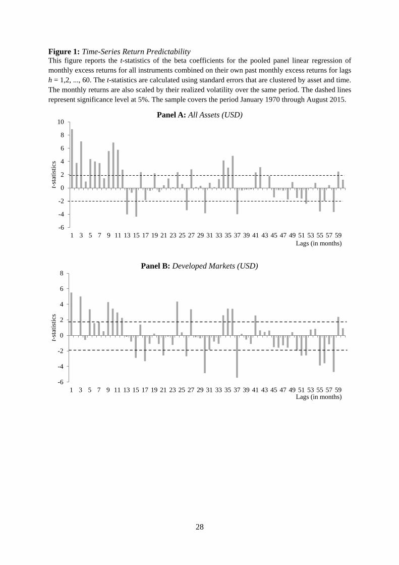
Figure 1: Time-Series Return Predictability This figure reports the t-statistics of the beta coefficients for the pooled panel linear regression of monthly excess returns for all instruments combined on their own past monthly excess returns for lags h = 1,2, ..., 60. The t-statistics are calculated using standard errors that are clustered by asset and time. The monthly returns are also scaled by their realized volatility over the same period. The dashed lines represent significance level at 5%. The sample covers the period January 1970 through August 2015.
-6
-4
-2
0
2
4
6
8
10
1 3 5 7 9 11 13 15 17 19 21 23 25 27 29 31 33 35 37 39 41 43 45 47 49 51 53 55 57 59
t-sta
tistic
s
Lags (in months)
Panel A: All Assets (USD)
-6
-4
-2
0
2
4
6
8
1 3 5 7 9 11 13 15 17 19 21 23 25 27 29 31 33 35 37 39 41 43 45 47 49 51 53 55 57 59
t-sta
tistic
s
Lags (in months)
Panel B: Developed Markets (USD)
28

-6
-4
-2
0
2
4
6
8
1 3 5 7 9 11 13 15 17 19 21 23 25 27 29 31 33 35 37 39 41 43 45 47 49 51 53 55 57 59
t-sta
tistic
s
Lags (in month)
Panel C: Emerging Markets (USD)
-6
-4
-2
0
2
4
6
8
10
1 3 5 7 9 11 13 15 17 19 21 23 25 27 29 31 33 35 37 39 41 43 45 47 49 51 53 55 57 59
t-sta
tistic
s
Lags (in months)
Panel D: Commodity Markets (USD)
29

Figure 2: International Equity and Commodity Funds Geographical Distribution We collect the universe of international mutual funds from Morningstar Direct from 1969 to 2015. Our dataset includes 1,177 international equity funds and 106 commodity funds. Panel A chart reports the investment areas in which the funds are concentrated. The classification is based on the Morningstar Category, Investment Area and Primary Prospectus Benchmark. Panel B chart reports the commodity sector in which the funds are concentrated. The classification is based on the Morningstar Category and Global Investment Funds Sectors (GIFS).
Panel A: International Equity Funds
Panel B: Commodity Funds Commodity Distribution
11112256991022233233
236245
539
0 100 200 300 400 500 600
UKCanada
KoreaScandinavia
European Emerging MarketsRussia & Commonwealth of Independent States (CIS)
AfricaIndiaJapan
Latin AmericaAsia Pacific
EuropeChina
United StatesAsia Pacific ex Japan
Global Emerging MarketsGlobal ex United States
Global
International Equity Funds - Investment Area Concetration
1
3
16
86
0 10 20 30 40 50 60 70 80 90 100
Energy
Agriculture
Precious Metals
Broad Basket
Commodity Funds - Holdings Distribution
30

Figure 3: Time-Series Currency Return Predictability This figure reports the t-statistics of the beta coefficients for the pooled panel linear regression of monthly returns of the currency components across all developed and emerging markets, combined separately, on their own past monthly returns for lags h = 1,2, ..., 36. The t-statistics are calculated using standard errors that are clustered by asset and time. The dashed lines represent significance level at 5%. The sample covers the period from January 1970 through August 2015.
Panel A: Developed Market Currency
Panel B: Emerging Market Currency
-10
-8
-6
-4
-2
0
2
4
6
8
1 3 5 7 9 11 13 15 17 19 21 23 25 27 29 31 33 35 37 39 41 43 45 47 49 51 53 55 57 59
t-sta
tistic
Lags (in months)
-6
-4
-2
0
2
4
6
8
10
12
14
16
1 3 5 7 9 11 13 15 17 19 21 23 25 27 29 31 33 35 37 39 41 43 45 47 49 51 53 55 57 59
t-sta
tistic
Lags (in months)
31

Figure 4: Mutual Fund Performance and Factors over Time Panel A graph reports the Newey-West t-statistics of the beta coefficients from the 36-month rolling multivariate regression of International Developed Market Mutual Fund returns on the MSCI World Index, the S&P GSCI Commodity Index, the single diversified 12-1 time-series momentum strategy (TSMOM), the winner and loser portfolios of the 12-1 time-series momentum strategy, the 12-1 long-only time-series momentum strategy, and the VAL and MOM factors. The sample covers the period starting from February 1971 through August 2015. Panel B reports the Newey-West t-statistics of the beta coefficients from the 36-month rolling multivariate regression of International Emerging Mutual Fund returns on the MSCI World Index, the S&P GSCI Commodity Index, the single diversified 12-1 time-series momentum strategy (TSMOM), the winner and loser portfolios of the 12-1 time-series momentum strategy, the 12-1 long-only time-series momentum strategy, and the VAL and MOM factors. The sample covers the period from October 1989 through August 2015. Panel C reports the t-statistics of the beta coefficients from the 36-month rolling multivariate regression of International Commodity Mutual Fund returns on the MSCI World Index, the S&P GSCI Commodity Index, the single diversified 12-1 time-series momentum strategy (TSMOM), the winner and loser portfolios of the 12-1 time-series momentum strategy, the 12-1 long-only time-series momentum strategy, and the VAL and MOM factors. The sample covers the period starting from November 1997 through August 2015.
Panel A: Developed Markets
-6
-4
-2
0
2
4
6
8
10
12
14
16
18
20
22
Dec-80 Dec-83 Dec-86 Dec-89 Dec-92 Dec-95 Dec-98 Dec-01 Dec-04 Dec-07 Dec-10 Dec-13
36-month Rolling t-statistics (Developed Markets)
MSCI World 12-1 TSMOM 12-1 TSMOM Winners12-1 TSMOM Losers Value Factor
32

Panel B: Emerging Markets
Panel C: Commodity Funds
-10
-8
-6
-4
-2
0
2
4
6
8
10
12
Sep-92 Sep-95 Sep-98 Sep-01 Sep-04 Sep-07 Sep-10 Sep-13
36-month Rolling t-statistics (Emerging Markets)
MSCI World 12-1 TSMOM 12-1 TSMOM Winners12-1 TSMOM Losers Value Factor
-10-8-6-4-202468
101214161820
Mar-00 Mar-03 Mar-06 Mar-09 Mar-12 Mar-15
36-month Rolling t-statistics (Commodity Markets)
S&P GSCI Index 12-1 TSMOM 12-1 TSMOM Winners12-1 TSMOM Losers Value Factor
33

Figure 5: Historical Performance of the Time-Series Momentum Strategy The figure presents the growth of a $100 investment in the single diversified 12-1 time-series momentum strategy and the MSCI World Index. The sample covers the period from January 1971 through August 2015. The figure also highlights the recession periods defined by the NBER; the oil crisis November 1973–March 1975, the “double dip” recession January 1980–July 1980, the early 1980s recession July 1981–November 1982, the oil price shock July 1990–March 1991, the dot-com bubble March 2001–November 2001 and the Great Recession December 2007–June 2009.
Figure 6: Option-like Behavior of Time-Series Momentum The figure presents the cumulative returns of the single diversified 12-1 time-series momentum strategy and the MSCI World Index during recession periods defined by NBER.
34

Figure 7: Time-Series Momentum “Smile” The figure presents the scatterplot of monthly returns of the single diversified 12-1 time-series momentum against the returns of the MSCI World Index. The dashed lines represent the quadratic fit. The sample covers the period January 1971 through August 2015.
-15%
-10%
-5%
0%
5%
10%
15%
20%
25%
30%
-25% -20% -15% -10% -5% 0% 5% 10% 15% 20%
12-1
TSM
OM
retu
rns
MSCI World returns
35
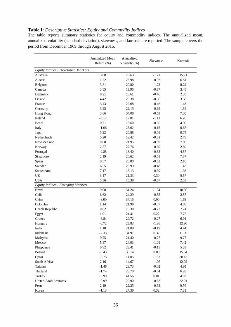
Table I: Descriptive Statistics: Equity and Commodity Indices The table reports summary statistics for equity and commodity indices. The annualized mean, annualized volatility (standard deviation), skewness, and kurtosis are reported. The sample covers the period from December 1969 through August 2015.
Annualized Mean Return (%)
Annualized Volatility (%)
Skewness Kurtosis
Australia 3.08 19.63 -1.71 15.71Austria 1.72 23.98 -0.92 6.51Belgium 3.81 20.80 -1.22 8.29Canada 3.85 19.95 -0.87 3.48Denmark 8.21 19.61 -0.46 2.33Finland 4.42 25.38 -0.36 3.38France 3.43 22.68 -0.46 1.48Germany 3.95 22.15 -0.65 1.84Hong Kong 3.66 34.08 -0.53 7.30Ireland -0.17 17.81 -1.11 6.28Israel 0.71 16.60 -0.55 4.90Italy -1.06 25.62 -0.15 0.67Japan 5.22 20.88 -0.01 0.74Netherlands 5.20 19.42 -0.81 2.79New Zealand 0.08 21.95 -0.99 7.89Norway 2.57 27.76 -0.80 2.89Portugal -2.85 18.40 -0.52 4.57Singapore 2.19 26.62 -0.61 7.37Spain 0.37 23.80 -0.52 2.18Sweden 6.55 23.99 -0.48 1.43Switzerland 7.17 18.13 -0.39 1.36UK 3.17 21.33 0.30 5.57USA 5.36 15.38 -0.67 2.53
Brazil 9.08 51.24 -1.34 10.86Chile 6.62 24.29 -0.55 2.57China -8.00 34.15 0.00 1.63Colombia 1.14 21.98 -0.37 4.88Czech Republic 0.62 19.30 -0.72 7.74Egypt 1.91 21.41 0.22 7.73Greece -6.84 29.72 -0.27 6.91Hungary -0.72 25.83 -1.36 12.90India 1.10 21.09 -0.19 4.44Indonesia -2.33 34.91 0.32 11.06Malaysia 0.25 21.40 -0.27 9.77Mexico 5.87 24.03 -1.01 7.42Philippines 0.92 23.41 -0.15 5.53Poland -0.43 30.14 0.88 15.54Qatar -0.73 14.05 -1.37 20.15South Africa 2.16 14.67 -1.06 12.02Taiwan -1.46 26.73 -0.02 4.95Thailand -1.74 28.70 -0.64 6.28Turkey -5.99 41.56 0.01 4.02United Arab Emirates -0.99 20.90 -0.62 22.01Peru 2.19 22.35 -0.83 9.56Korea -1.13 27.39 0.32 7.31
Equity Indices - Emerging Markets
Equity Indices - Developed Markets
36

Table I (Continued)
Crude Oil -1.67 32.92 -0.15 1.61Gold -1.72 15.57 -0.03 1.41Brent Crude Oil 3.13 32.00 -0.64 2.09Copper 0.16 27.38 -0.37 4.23Natural Gas -35.87 51.41 -0.06 0.63Live Stock 0.03 13.74 -0.49 0.62Corn -8.13 27.00 0.22 2.13Silver -6.54 28.16 -0.13 1.37Zinc -3.38 25.40 -0.50 3.55Sugar -11.27 31.75 0.03 0.78Soybeans -0.47 23.88 -0.29 1.11Cocoa -7.20 28.35 0.18 0.76Heating Oil -1.51 31.40 -0.01 1.19Aluminum -3.93 19.14 -0.06 0.54Nickel -4.09 34.33 -0.14 0.43Coffee -8.86 36.33 0.52 1.84Lean Hogs -5.64 24.12 -0.37 0.84Palladium 0.21 35.35 -0.25 2.30Petroleum -0.66 30.87 -0.17 1.73Wheat -8.26 27.04 0.02 1.43Cotton -4.62 25.87 -0.05 0.73Live Cattle 1.49 13.12 -0.82 4.40
Commodity Indices
37

Table II: International Equity and Commodity Funds Descriptive Statistics The table reports sample descriptive statistics for the funds that existed at any time between December 1968 and August 2015, with the total sample including 1177 international equity funds and 106 commodity funds. Monthly Net Cash Flow for fund j in month t is computed as NCFj,t = NCFj,t-[NCFj,t-1(1+rj,t)]. Statistics for commodity funds concern shorter data starting from April 1997, alongside that for Total Net Assets and Net Cash Flow; for equity funds data starts from January 1990. Statistics are based on the monthly cross-sectional mean for each measure.
Panel A: International Equity Funds (Developed Markets)
Mean Median 25th
Percentile75th
PercentileMax Min
Standard Deviation
Total Net Assets ($ millions) 823.05 691.74 351.90 1248.20 2565.87 19.48 565.71
Monthly Net Cash Flow ($ millions) -3.19 0.53 -29.92 26.77 148.26 -160.97 50.80
Expense Ratio (%/year) 1.40 1.37 1.30 1.44 2.37 1.14 0.23
Turover (%/year) 63.68 63.05 58.10 73.04 88.28 12.90 14.88
Fund Age (years) 13.08 10.67 5.85 19.73 46.75 0.00 9.10
Monthly Allocation to Equity (%) 93.92 94.89 92.23 96.11 107.60 76.65 3.66
Monthly Allocation to non-US Equity (%) 65.40 68.59 60.59 73.37 97.60 0.00 15.31
Monthly Net Return (%) 0.84 1.01 -1.69 3.93 13.63 -22.48 4.54
Monthly Gross Return (%) 0.96 1.12 -1.58 4.05 13.76 -22.39 4.54
Panel B: International Equity Funds (Emerging Markets)
Mean Median 25th
Percentile75th
PercentileMax Min
Standard Deviation
Total Net Assets ($ millions) 1153.94 1140.85 939.13 1275.56 2225.71 1.50 311.28
Monthly Net Cash Flow ($ millions) -7.90 1.64 -46.93 47.33 293.52 -332.28 93.97
Expense Ratio (%/year) 1.57 1.55 1.43 1.71 2.37 0.98 0.29
Turover (%/year) 53.32 57.17 44.34 67.35 88.66 9.43 22.42
Fund Age (years) 8.82 4.92 1.92 15.04 46.75 0.00 8.93
Monthly Allocation to Equity (%) 90.54 92.21 87.96 94.63 99.94 71.62 5.12
Monthly Allocation to non-US Equity (%) 76.12 79.24 73.75 82.67 144.61 0.00 11.31
Monthly Net Return (%) 1.11 1.39 -1.65 4.17 16.92 -26.86 5.26
Monthly Gross Return (%) 1.25 1.51 -1.52 4.29 17.07 -26.75 5.27
Panel C: Commodity Funds
Mean Median 25th
Percentile75th
PercentileMax Min
Standard Deviation
Total Net Assets ($ millions) 575.20 561.96 130.27 854.42 1954.84 1.40 450.25
Monthly Net Cash Flow ($ millions) 18.59 7.92 -5.10 35.35 384.22 -172.19 64.41
Expense Ratio (%/year) 1.48 1.51 1.34 1.65 1.82 1.07 0.21
Turover (%/year) 101.13 10.95 1.22 68.08 1140.85 -7.90 283.11
Fund Age (years) 6.20 5.25 3.75 8.50 18.50 1.25 3.50
Monthly Allocation to Cash (%) 47.44 46.01 38.85 53.23 90.37 4.87 13.94
Monthly Allocation to Equity (%) 12.41 11.53 6.88 18.35 70.43 -0.04 10.56
Monthly Net Return (%) 0.26 0.37 -3.33 3.82 15.25 -24.46 5.55
Monthly Gross Return (%) 0.37 0.45 -3.26 4.03 15.37 -24.33 5.58
38

Table III: Time-Series Momentum Strategies across All Asset Classes The table reports the annualized mean returns and the annualized Sharpe ratios for time-series momentum strategies across all asset classes in USD with a look-back period of J months and a holding period of K months. The sample covers the period January 1970 through August 2015. Significance at the 1% and 5% are denoted as *** and **, respectively.
Panel A : All assets
K 1 3 6 9 12 24 36 1 3 6 9 12 24 36
J
1 8.73*** 4.66*** 3.17*** 2.67*** 2.30*** 1.33*** 1.09*** 0.68 0.72 0.78 0.78 0.77 0.61 0.57
3 10.16*** 4.91*** 4.03*** 3.91*** 2.92*** 1.57*** 1.57*** 0.64 0.58 0.65 0.73 0.64 0.47 0.51
6 11.48*** 6.42*** 5.66*** 4.53*** 3.29*** 1.94*** 1.81*** 0.68 0.66 0.72 0.66 0.54 0.45 0.45
9 12.82*** 7.57*** 5.41*** 3.78*** 2.92*** 1.81** 1.81*** 0.77 0.72 0.63 0.51 0.44 0.35 0.41
12 11.88*** 6.29*** 4.03*** 2.92*** 2.30** 1.57 1.69** 0.69 0.59 0.46 0.39 0.34 0.29 0.34
24 4.28 1.94 0.96 0.84 0.96 1.33 1.33 0.27 0.19 0.11 0.10 0.12 0.20 0.23
36 4.41 2.43 1.69 1.69 1.69 1.45 1.33 0.29 0.24 0.19 0.22 0.23 0.22 0.21
Panel B : Equity Index
K 1 3 6 9 12 24 36 1 3 6 9 12 24 36
J
1 9.77*** 5.28*** 3.78*** 3.17*** 2.67*** 1.69*** 1.57*** 0.62 0.65 0.71 0.71 0.69 0.59 0.57
3 10.82*** 5.28*** 4.53*** 4.41*** 3.54*** 2.18** 2.06*** 0.55 0.47 0.58 0.63 0.58 0.47 0.50
6 12.95*** 7.57*** 6.68*** 5.28*** 3.91*** 2.67** 2.43 0.60 0.60 0.65 0.59 0.50 0.45 0.44
9 14.98*** 8.73*** 6.29*** 4.53*** 3.54** 2.55 2.55 0.69 0.64 0.57 0.47 0.41 0.37 0.42
12 13.22*** 7.31*** 4.91*** 3.66 2.92 2.43 2.43 0.59 0.53 0.44 0.37 0.32 0.33 0.35
24 5.16 2.67 1.69 1.57 1.94 2.30 2.18 0.25 0.20 0.14 0.15 0.19 0.26 0.27
36 6.17 3.54 2.80 3.04 3.04 2.67 2.18 0.32 0.28 0.26 0.30 0.32 0.29 0.25
Annualized mean return (%) Annualized Sharpe ratio
Annualized mean return (%) Annualized Sharpe ratio
39
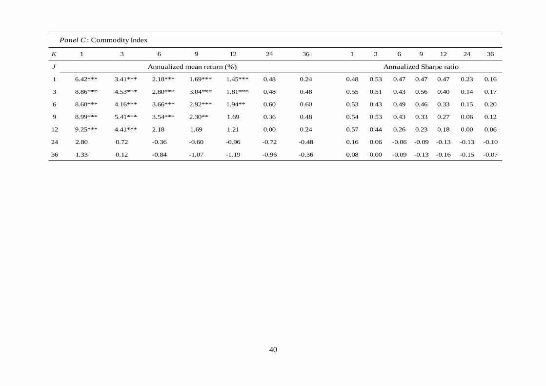
K 1 3 6 9 12 24 36 1 3 6 9 12 24 36
J
1 6.42*** 3.41*** 2.18*** 1.69*** 1.45*** 0.48 0.24 0.48 0.53 0.47 0.47 0.47 0.23 0.16
3 8.86*** 4.53*** 2.80*** 3.04*** 1.81*** 0.48 0.48 0.55 0.51 0.43 0.56 0.40 0.14 0.17
6 8.60*** 4.16*** 3.66*** 2.92*** 1.94** 0.60 0.60 0.53 0.43 0.49 0.46 0.33 0.15 0.20
9 8.99*** 5.41*** 3.54*** 2.30** 1.69 0.36 0.48 0.54 0.53 0.43 0.33 0.27 0.06 0.12
12 9.25*** 4.41*** 2.18 1.69 1.21 0.00 0.24 0.57 0.44 0.26 0.23 0.18 0.00 0.06
24 2.80 0.72 -0.36 -0.60 -0.96 -0.72 -0.48 0.16 0.06 -0.06 -0.09 -0.13 -0.13 -0.10
36 1.33 0.12 -0.84 -1.07 -1.19 -0.96 -0.36 0.08 0.00 -0.09 -0.13 -0.16 -0.15 -0.07
Panel C : Commodity Index
Annualized mean return (%) Annualized Sharpe ratio
40
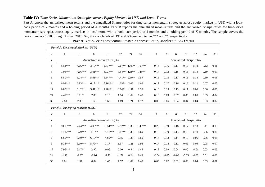
Table IV: Time-Series Momentum Strategies across Equity Markets in USD and Local Terms Part A reports the annualized mean returns and the annualized Sharpe ratios for time-series momentum strategies across equity markets in USD with a look-back period of J months and a holding period of K months. Park B reports the annualized mean returns and the annualized Sharpe ratios for time-series momentum strategies across equity markets in local terms with a look-back period of J months and a holding period of K months. The sample covers the period January 1970 through August 2015. Significance levels of 1% and 5% are denoted as *** and **, respectively.
Part A: Time-Series Momentum Strategies across Equity Markets in USD terms
K 1 3 6 9 12 24 36 1 3 6 9 12 24 36
J
1 5.54*** 4.66*** 3.17*** 2.67*** 2.67*** 1.45*** 1.09*** 0.14 0.16 0.17 0.17 0.18 0.12 0.11
3 7.06*** 4.66*** 3.91*** 4.03*** 3.54*** 1.69*** 1.45** 0.14 0.13 0.15 0.16 0.14 0.10 0.09
6 6.80*** 6.04*** 5.91*** 5.54*** 4.41*** 2.30*** 1.57 0.16 0.15 0.17 0.16 0.14 0.10 0.08
9 6.93*** 6.93*** 6.17*** 5.16*** 4.03*** 2.06 1.69 0.17 0.17 0.16 0.13 0.11 0.07 0.07
12 6.80*** 6.42*** 5.41*** 4.28*** 3.04** 1.57 1.33 0.16 0.15 0.13 0.11 0.08 0.06 0.06
24 4.41*** 3.91** 2.80 2.18 1.94 1.69 1.45 0.10 0.09 0.07 0.06 0.05 0.05 0.04
36 2.80 2.30 1.69 1.69 1.69 1.21 0.72 0.06 0.05 0.04 0.04 0.04 0.03 0.02
K 1 3 6 9 12 24 36 1 3 6 9 12 24 36
J
1 10.03*** 7.44*** 4.03*** 3.54*** 2.92*** 1.33 1.45*** 0.22 0.19 0.18 0.17 0.13 0.11 0.13
3 11.22*** 5.79*** 4.16** 4.41*** 3.17** 1.33 1.69 0.15 0.10 0.13 0.13 0.10 0.06 0.10
6 8.60*** 6.80*** 6.17*** 4.66** 2.55 1.33 1.69 0.14 0.13 0.14 0.10 0.05 0.06 0.08
9 9.38*** 8.60*** 5.79** 3.17 1.57 1.21 1.94 0.17 0.14 0.11 0.05 0.03 0.05 0.07
12 7.96*** 6.17** 2.92 0.96 0.00 0.84 1.45 0.12 0.09 0.04 0.00 -0.01 0.03 0.05
24 -1.43 -2.37 -2.96 -2.73 -1.79 0.24 0.48 -0.04 -0.05 -0.06 -0.05 -0.03 0.01 0.02
36 1.81 1.57 0.84 1.45 1.57 1.09 0.48 0.03 0.02 0.02 0.03 0.04 0.03 0.01
Panel A: Developed Markets (USD)
Annualized mean return (%) Annualized Sharpe ratio
Panel B: Emerging Markets (USD)
Annualized mean return (%) Annualized Sharpe ratio
41

Part B: Time-Series Momentum Strategies across Equity Markets in Local Terms
K 1 3 6 9 12 24 36 1 3 6 9 12 24 36
J
1 6.17*** 4.53*** 3.41*** 3.04*** 3.17*** 1.57*** 1.21*** 0.18 0.20 0.19 0.21 0.21 0.13 0.11
3 6.68*** 5.16*** 4.16*** 4.53*** 4.03*** 2.18*** 1.69*** 0.16 0.16 0.16 0.19 0.17 0.12 0.11
6 7.44*** 5.79*** 6.04*** 5.79*** 4.66*** 2.43*** 1.69** 0.17 0.17 0.19 0.18 0.16 0.11 0.08
9 7.44*** 7.19*** 6.93*** 5.79*** 4.53*** 2.30** 1.81 0.20 0.20 0.19 0.16 0.13 0.08 0.08
12 8.21*** 7.06*** 5.79*** 4.78*** 3.66*** 1.94 1.45 0.19 0.17 0.15 0.13 0.11 0.07 0.06
24 4.53*** 4.03*** 3.29** 2.80 2.30 1.57 1.45 0.11 0.10 0.09 0.07 0.06 0.05 0.05
36 3.29** 2.80 2.06 1.81 1.81 1.69 1.45 0.09 0.08 0.06 0.05 0.05 0.05 0.04
K 1 3 6 9 12 24 36 1 3 6 9 12 24 36
J
1 9.38*** 7.57*** 4.66*** 4.53*** 3.91*** 2.30*** 2.18*** 0.36 0.34 0.36 0.37 0.35 0.35 0.37
3 9.9*** 6.55*** 5.28*** 5.41*** 4.28*** 2.43*** 2.43*** 0.27 0.24 0.28 0.31 0.29 0.30 0.33
6 8.73*** 6.93*** 6.93*** 6.04*** 4.03*** 2.92*** 2.80*** 0.23 0.24 0.27 0.26 0.22 0.27 0.28
9 10.16*** 9.25*** 7.06*** 5.16*** 3.54** 3.17** 3.29*** 0.27 0.26 0.23 0.20 0.19 0.24 0.26
12 9.25*** 7.06** 4.78** 3.54 2.55 3.04** 3.04*** 0.24 0.21 0.18 0.16 0.16 0.22 0.23
24 2.92 2.06 1.57 1.33 1.81 3.04 2.92 0.13 0.12 0.11 0.12 0.14 0.18 0.18
36 6.04 5.54 4.41 4.28 4.28 4.16 3.66 0.23 0.21 0.19 0.20 0.20 0.20 0.18
Panel B: Emerging Markets (Local)
Annualized mean return (%) Annualized Sharpe ratio
Panel A: Developed Markets (Local)
Annualized mean return (%) Annualized Sharpe ratio
42

Table V: Performance of the Diversified 12-1 Time-Series Momentum Strategy-1 The table presents the beta coefficients and their respective t-statistics from regressing the equally weighted average across instruments return of the single diversified 12-1 time-series momentum strategy on (i) the monthly MSCI World Index return, (ii) the monthly S&P GSCI Index return, and (iii) the SMB, HML and UMD which denote the Fama-French factors representing size, value and momentum across U.S. stocks. The sample covers the period from January 1970 through August 2015.
Intercept MSCI GSCI SMB HML UMD R2
Coefficient 0.29% 0.04 -0.01 0.02 0.05 0.30 20.78%
(t -statistic) (2.52) (1.52) (-0.77) (0.66) (1.14) (11.65)
Intercept MSCI GSCI SMB HML UMD R2
Coefficient 0.23% 0.08 -0.05 0.03 0.08 0.39 19.95%
(t -statistic) (1.54) (2.21) (-1.98) (0.62) (1.53) (11.41)
Intercept MSCI GSCI SMB HML UMD R2
Coefficient 0.20% 0.08 -0.07 0.05 0.04 0.36 17.15%
(t -statistic) (1.26) (2.27) (-2.63) (1.10) (0.78) (10.18)
Intercept MSCI GSCI SMB HML UMD R2
Coefficient 0.30% -0.01 -0.06 -0.04 0.12 0.46 21.23%
(t -statistic) (1.17) (-0.22) (-1.32) (-0.53) (1.38) (8.53)
Intercept MSCI GSCI SMB HML UMD R2
Coefficient 0.44% -0.03 0.10 0.01 -0.05 0.12 7.04%
(t -statistic) (3.09) (-0.85) (4.19) (0.18) (-1.02) (3.88)
Panel C: Commodity Index
Panel A: All Assets
Panel B: Equity Index (All)
Developed Markets
Emerging Markets
43
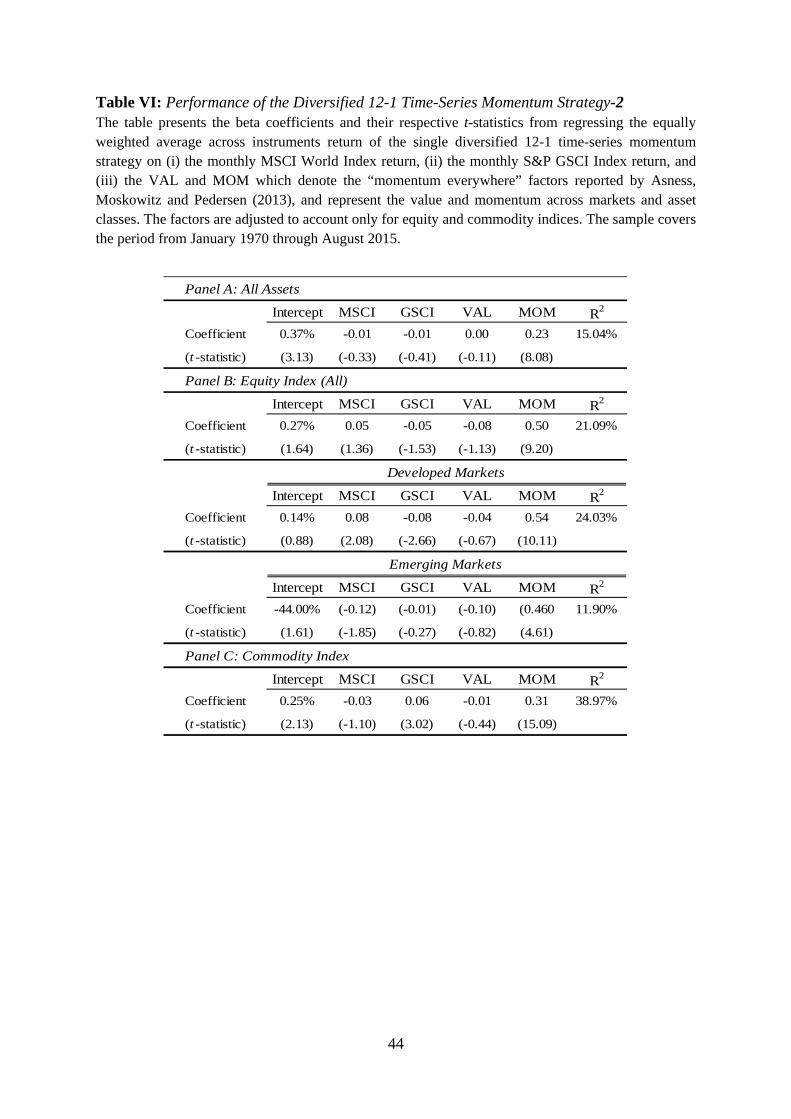
Table VI: Performance of the Diversified 12-1 Time-Series Momentum Strategy-2 The table presents the beta coefficients and their respective t-statistics from regressing the equally weighted average across instruments return of the single diversified 12-1 time-series momentum strategy on (i) the monthly MSCI World Index return, (ii) the monthly S&P GSCI Index return, and (iii) the VAL and MOM which denote the “momentum everywhere” factors reported by Asness, Moskowitz and Pedersen (2013), and represent the value and momentum across markets and asset classes. The factors are adjusted to account only for equity and commodity indices. The sample covers the period from January 1970 through August 2015.
Intercept MSCI GSCI VAL MOM R2
Coefficient 0.37% -0.01 -0.01 0.00 0.23 15.04%
(t -statistic) (3.13) (-0.33) (-0.41) (-0.11) (8.08)
Intercept MSCI GSCI VAL MOM R2
Coefficient 0.27% 0.05 -0.05 -0.08 0.50 21.09%
(t -statistic) (1.64) (1.36) (-1.53) (-1.13) (9.20)
Intercept MSCI GSCI VAL MOM R2
Coefficient 0.14% 0.08 -0.08 -0.04 0.54 24.03%
(t -statistic) (0.88) (2.08) (-2.66) (-0.67) (10.11)
Intercept MSCI GSCI VAL MOM R2
Coefficient -44.00% (-0.12) (-0.01) (-0.10) (0.460 11.90%
(t -statistic) (1.61) (-1.85) (-0.27) (-0.82) (4.61)
Intercept MSCI GSCI VAL MOM R2
Coefficient 0.25% -0.03 0.06 -0.01 0.31 38.97%
(t -statistic) (2.13) (-1.10) (3.02) (-0.44) (15.09)
Panel A: All Assets
Panel B: Equity Index (All)
Developed Markets
Emerging Markets
Panel C: Commodity Index
44
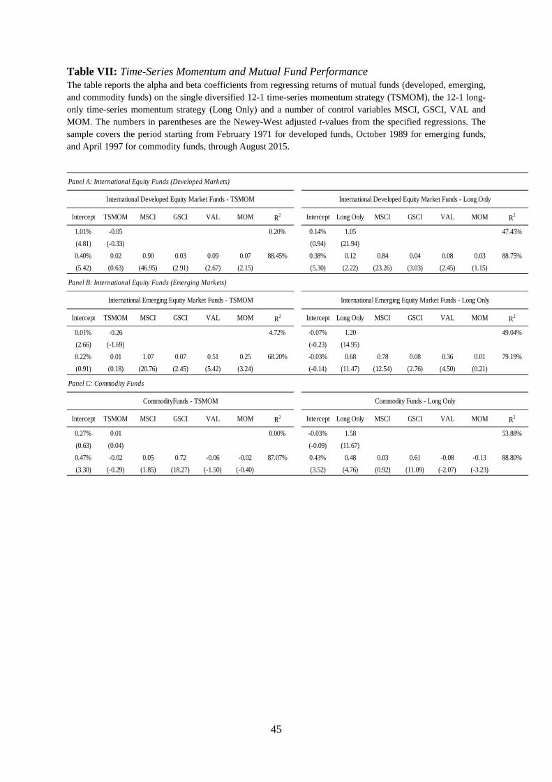
Table VII: Time-Series Momentum and Mutual Fund Performance The table reports the alpha and beta coefficients from regressing returns of mutual funds (developed, emerging, and commodity funds) on the single diversified 12-1 time-series momentum strategy (TSMOM), the 12-1 long-only time-series momentum strategy (Long Only) and a number of control variables MSCI, GSCI, VAL and MOM. The numbers in parentheses are the Newey-West adjusted t-values from the specified regressions. The sample covers the period starting from February 1971 for developed funds, October 1989 for emerging funds, and April 1997 for commodity funds, through August 2015.
Panel A: International Equity Funds (Developed Markets)
Intercept TSMOM MSCI GSCI VAL MOM R2 Intercept Long Only MSCI GSCI VAL MOM R2
1.01% -0.05 0.20% 0.14% 1.05 47.45%(4.81) (-0.33) (0.94) (21.94)0.40% 0.02 0.90 0.03 0.09 0.07 88.45% 0.38% 0.12 0.84 0.04 0.08 0.03 88.75%(5.42) (0.63) (46.95) (2.91) (2.67) (2.15) (5.30) (2.22) (23.26) (3.03) (2.45) (1.15)
Panel B: International Equity Funds (Emerging Markets)
Intercept TSMOM MSCI GSCI VAL MOM R2 Intercept Long Only MSCI GSCI VAL MOM R2
0.01% -0.26 4.72% -0.07% 1.20 49.04%(2.66) (-1.69) (-0.23) (14.95)0.22% 0.01 1.07 0.07 0.51 0.25 68.20% -0.03% 0.68 0.78 0.08 0.36 0.01 79.19%(0.91) (0.18) (20.76) (2.45) (5.42) (3.24) (-0.14) (11.47) (12.54) (2.76) (4.50) (0.21)
Panel C: Commodity Funds
Intercept TSMOM MSCI GSCI VAL MOM R2 Intercept Long Only MSCI GSCI VAL MOM R2
0.27% 0.01 0.00% -0.03% 1.58 53.88%(0.63) (0.04) (-0.09) (11.67)0.47% -0.02 0.05 0.72 -0.06 -0.02 87.07% 0.43% 0.48 0.03 0.61 -0.08 -0.13 88.80%(3.30) (-0.29) (1.85) (18.27) (-1.50) (-0.40) (3.52) (4.76) (0.92) (11.09) (-2.07) (-3.23)
International Developed Equity Market Funds - TSMOM International Developed Equity Market Funds - Long Only
International Emerging Equity Market Funds - TSMOM International Emerging Equity Market Funds - Long Only
CommodityFunds - TSMOM Commodity Funds - Long Only
45
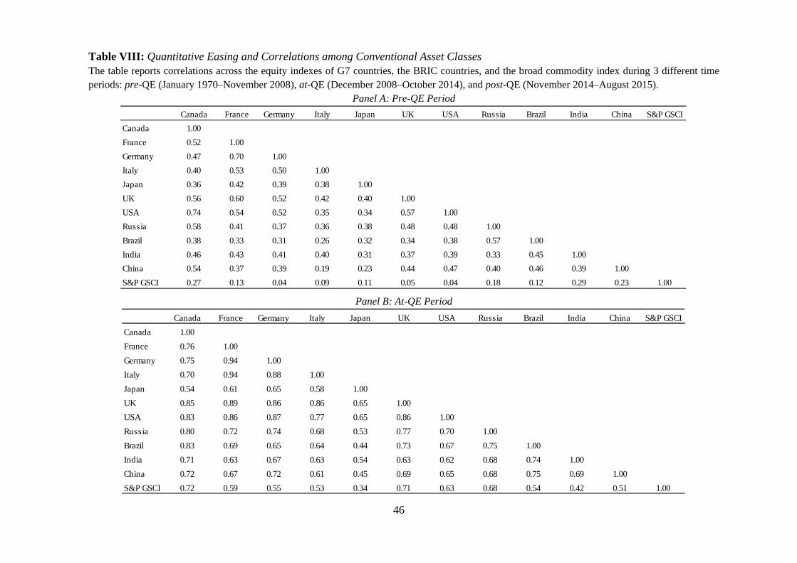
Table VIII: Quantitative Easing and Correlations among Conventional Asset Classes The table reports correlations across the equity indexes of G7 countries, the BRIC countries, and the broad commodity index during 3 different time periods: pre-QE (January 1970–November 2008), at-QE (December 2008–October 2014), and post-QE (November 2014–August 2015).
Panel A: Pre-QE Period
Panel B: At-QE Period
Canada France Germany Italy Japan UK USA Russia Brazil India China S&P GSCICanada 1.00France 0.52 1.00Germany 0.47 0.70 1.00Italy 0.40 0.53 0.50 1.00Japan 0.36 0.42 0.39 0.38 1.00UK 0.56 0.60 0.52 0.42 0.40 1.00USA 0.74 0.54 0.52 0.35 0.34 0.57 1.00Russia 0.58 0.41 0.37 0.36 0.38 0.48 0.48 1.00Brazil 0.38 0.33 0.31 0.26 0.32 0.34 0.38 0.57 1.00India 0.46 0.43 0.41 0.40 0.31 0.37 0.39 0.33 0.45 1.00China 0.54 0.37 0.39 0.19 0.23 0.44 0.47 0.40 0.46 0.39 1.00S&P GSCI 0.27 0.13 0.04 0.09 0.11 0.05 0.04 0.18 0.12 0.29 0.23 1.00
Canada France Germany Italy Japan UK USA Russia Brazil India China S&P GSCICanada 1.00France 0.76 1.00Germany 0.75 0.94 1.00Italy 0.70 0.94 0.88 1.00Japan 0.54 0.61 0.65 0.58 1.00UK 0.85 0.89 0.86 0.86 0.65 1.00USA 0.83 0.86 0.87 0.77 0.65 0.86 1.00Russia 0.80 0.72 0.74 0.68 0.53 0.77 0.70 1.00Brazil 0.83 0.69 0.65 0.64 0.44 0.73 0.67 0.75 1.00India 0.71 0.63 0.67 0.63 0.54 0.63 0.62 0.68 0.74 1.00China 0.72 0.67 0.72 0.61 0.45 0.69 0.65 0.68 0.75 0.69 1.00S&P GSCI 0.72 0.59 0.55 0.53 0.34 0.71 0.63 0.68 0.54 0.42 0.51 1.00
46

Panel C: Post-QE Period
Canada France Germany Italy Japan UK USA Russia Brazil India China S&P GSCICanada 1.00France 0.62 1.00Germany 0.43 0.87 1.00Italy 0.56 0.91 0.73 1.00Japan 0.59 0.81 0.71 0.82 1.00UK 0.74 0.88 0.62 0.80 0.82 1.00USA 0.70 0.78 0.73 0.71 0.77 0.82 1.00Russia 0.58 0.60 0.38 0.80 0.65 0.57 0.33 1.00Brazil 0.75 0.54 0.32 0.49 0.53 0.66 0.35 0.69 1.00India -0.22 0.45 0.58 0.44 0.50 0.33 0.38 0.12 -0.01 1.00China 0.65 0.44 0.35 0.32 0.67 0.57 0.37 0.44 0.67 -0.05 1.00S&P GSCI 0.55 0.18 -0.10 0.41 0.31 0.35 0.06 0.83 0.70 -0.23 0.40 1.00
47
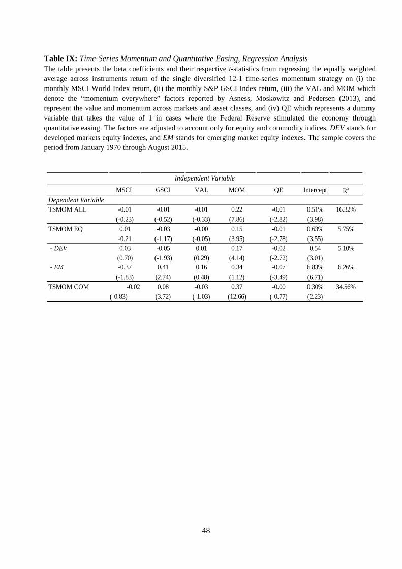
Table IX: Time-Series Momentum and Quantitative Easing, Regression Analysis The table presents the beta coefficients and their respective t-statistics from regressing the equally weighted average across instruments return of the single diversified 12-1 time-series momentum strategy on (i) the monthly MSCI World Index return, (ii) the monthly S&P GSCI Index return, (iii) the VAL and MOM which denote the “momentum everywhere” factors reported by Asness, Moskowitz and Pedersen (2013), and represent the value and momentum across markets and asset classes, and (iv) QE which represents a dummy variable that takes the value of 1 in cases where the Federal Reserve stimulated the economy through quantitative easing. The factors are adjusted to account only for equity and commodity indices. DEV stands for developed markets equity indexes, and EM stands for emerging market equity indexes. The sample covers the period from January 1970 through August 2015.
MSCI GSCI VAL MOM QE Intercept R2
Dependent VariableTSMOM ALL -0.01 -0.01 -0.01 0.22 -0.01 0.51% 16.32%
(-0.23) (-0.52) (-0.33) (7.86) (-2.82) (3.98)TSMOM EQ 0.01 -0.03 -0.00 0.15 -0.01 0.63% 5.75%
-0.21 (-1.17) (-0.05) (3.95) (-2.78) (3.55) - DEV 0.03 -0.05 0.01 0.17 -0.02 0.54 5.10%
(0.70) (-1.93) (0.29) (4.14) (-2.72) (3.01) - EM -0.37 0.41 0.16 0.34 -0.07 6.83% 6.26%
(-1.83) (2.74) (0.48) (1.12) (-3.49) (6.71)TSMOM COM -0.02 0.08 -0.03 0.37 -0.00 0.30% 34.56%
(-0.83) (3.72) (-1.03) (12.66) (-0.77) (2.23)
Independent Variable
48


