

The Trimmed Lasso: Sparsity and Robustness
Dimitris Bertsimas, Martin S. Copenhaver, and Rahul Mazumder∗
August 15, 2017
Abstract
Nonconvex penalty methods for sparse modeling in linear regression have been a topic offervent interest in recent years. Herein, we study a family of nonconvex penalty functions thatwe call the trimmed Lasso and that offers exact control over the desired level of sparsity ofestimators. We analyze its structural properties and in doing so show the following:
1. Drawing parallels between robust statistics and robust optimization, we show that thetrimmed-Lasso-regularized least squares problem can be viewed as a generalized form oftotal least squares under a specific model of uncertainty. In contrast, this same modelof uncertainty, viewed instead through a robust optimization lens, leads to the convexSLOPE (or OWL) penalty.
2. Further, in relating the trimmed Lasso to commonly used sparsity-inducing penalty func-tions, we provide a succinct characterization of the connection between trimmed-Lasso-like approaches and penalty functions that are coordinate-wise separable, showing thatthe trimmed penalties subsume existing coordinate-wise separable penalties, with strictcontainment in general.
3. Finally, we describe a variety of exact and heuristic algorithms, both existing and new,for trimmed Lasso regularized estimation problems. We include a comparison between thedifferent approaches and an accompanying implementation of the algorithms.
1 Introduction
Sparse modeling in linear regression has been a topic of fervent interest in recent years [23, 42].This interest has taken several forms, from substantial developments in the theory of the Lasso toadvances in algorithms for convex optimization. Throughout there has been a strong emphasis onthe increasingly high-dimensional nature of linear regression problems; in such problems, where thenumber of variables p can vastly exceed the number of observations n, sparse modeling techniquesare critical for performing inference.
Context
One of the fundamental approaches to sparse modeling in the usual linear regression model ofy = Xβ + ε, with y ∈ Rn and X ∈ Rn×p, is the best subset selection [57] problem:
min‖β‖0≤k
1
2‖y −Xβ‖22, (1)
∗Authors’ affiliation: Sloan School of Management and Operations Research Center, MIT.Emails: {dbertsim,mcopen,rahulmaz}@mit.edu.
1

which seeks to find the best choice of k from among p features that best explain the response interms of the least squares loss function. The problem (1) has received extensive attention froma variety of statistical and optimization perspectives—see for example [14] and references therein.One can also consider the Lagrangian, or penalized, form of (1), namely,
minβ
1
2‖y −Xβ‖22 + µ‖β‖0, (2)
for a regularization parameter µ > 0. One of the advantages of (1) over (2) is that it offers directcontrol over estimators’ sparsity via the discrete parameter k, as opposed to the Lagrangian form(2) for which the correspondence between the continuous parameter µ and the resulting sparsity ofestimators obtained is not entirely clear. For further discussion, see [65].
Another class of problems that have received considerable attention in the statistics and machinelearning literature is the following:
minβ
1
2‖y −Xβ‖22 +R(β), (3)
where R(β) is a choice of regularizer which encourages sparsity in β. For example, the popularlyused Lasso [70] takes the form of problem (3) with R(β) = µ‖β‖1, where ‖ · ‖1 is the `1 norm; indoing so, the Lasso simultaneously selects variables and also performs shrinkage. The Lasso hasseen widespread success across a variety of applications.
In contrast to the convex approach of the Lasso, there also has been been growing interest inconsidering richer classes of regularizers R which include nonconvex functions. Examples of suchpenalties include the `q-penalty (for q ∈ [0, 1]), minimax concave penalty (MCP) [74], and thesmoothly clipped absolute deviation (SCAD) [33], among others. Many of the nonconvex penaltyfunctions considered are coordinate-wise separable; in other words, R can be decomposed as
R(β) =
p∑i=1
ρ(|βi|),
where ρ(·) is a real-valued function [75]. There has been a variety of evidence suggesting the promiseof such nonconvex approaches in overcoming certain shortcomings of Lasso-like approaches.
One of the central ideas of nonconvex penalty methods used in sparse modeling is that ofcreating a continuum of estimation problems which bridge the gap between convex methods forsparse estimation (such as Lasso) and subset selection in the form (1). However, as noted above,such a connection does not necessarily offer direct control over the desired level of sparsity ofestimators.
The trimmed Lasso
In contrast with coordinate-wise separable penalties as considered above, we consider a family ofpenalties that are not separable across coordinates. One such penalty which forms a principalobject of our study herein is
Tk (β) := min‖φ‖0≤k
‖φ− β‖1.
The penalty Tk is a measure of the distance from the set of k-sparse estimators as measured viathe `1 norm. In other words, when used in problem (3), the penalty R = Tk controls the amountof shrinkage towards sparse models.
2

The penalty Tk can equivalently be written as
Tk (β) =
p∑i=k+1
|β(i)|,
where |β(1)| ≥ |β(2)| ≥ · · · ≥ |β(p)| are the sorted entries of β. In words, Tk (β) is the sum of theabsolute values of the p − k smallest magnitude entries of β. The penalty was first introducedin [39, 43, 69, 72]. We refer to this family of penalty functions (over choices of k) as the trimmedLasso.1 The case of k = 0 recovers the usual Lasso, as one would suspect. The distinction, ofcourse, is that for general k, Tk no longer shrinks, or biases towards zero, the k largest entries of β.
Let us consider the least squares loss regularized via the trimmed lasso penalty—this leads tothe following optimization criterion:
minβ
1
2‖y −Xβ‖22 + λTk (β) , (4)
where λ > 0 is the regularization parameter. The penalty term shrinks the smallest p−k entries ofβ and does not impose any penalty on the largest k entries of β. If λ becomes larger, the smallestp − k entries of β are shrunk further; after a certain threshold—as soon as λ ≥ λ0 for some finiteλ0—the smallest p − k entries are set to zero. The existence of a finite λ0 (as stated above) isan attractive feature of the trimmed Lasso and is known as its exactness property, namely, for λsufficiently large, the problem (4) exactly solves constrained best subset selection as in problem (1)(c.f. [39]). Note here the contrast with the separable penalty functions which correspond insteadwith problem (2); as such, the trimmed Lasso is distinctive in that it offers precise control over thedesired level of sparsity vis-a-vis the discrete parameter k. Further, it is also notable that manyalgorithms developed for separable-penalty estimation problems can be directly adapted for thetrimmed Lasso.
Our objective in studying the trimmed Lasso is distinctive from previous approaches. In par-ticular, while previous work on the penalty Tk has focused primarily on its use as a tool forreformulating sparse optimization problems [43, 69] and on how such reformulations can be solvedcomputationally [39, 72], we instead aim to explore the trimmed Lasso’s structural properties andits relation to existing sparse modeling techniques.
In particular, a natural question we seek to explore is, what is the connection of the trimmedLasso penalty with existing separable penalties commonly used in sparse statistical learning? Forexample, the trimmed Lasso bears a close resemblance to the clipped (or capped) Lasso penalty [76],namely,
p∑i=1
µmin{γ|βi|, 1},
where µ, γ > 0 are parameters (when γ is large, the clipped Lasso approximates µ‖β‖0).
Robustness: robust statistics and robust optimization
A significant thread woven throughout the consideration of penalty methods for sparse modelingis the notion of robustness—in short, the ability of a method to perform in the face of noise.Not surprisingly, the notion of robustness has myriad distinct meanings depending on the context.Indeed, as Huber, a pioneer in the area of robust statistics, aptly noted:
1The choice of name is our own and is motivated by the least trimmed squares regression estimator, describedbelow
3

“The word ‘robust’ is loaded with many—sometimes inconsistent—connotations.” [45,p. 2]
For this reason, we consider robustness from several perspectives—both the robust statistics [45]and robust optimization [9] viewpoints.
A common premise of the various approaches is as follows: that a robust model should performwell even under small deviations from its underlying assumptions; and that to achieve such behavior,some efficiency under the assumed model should be sacrificed. Not surprisingly in light of Huber’sprescient observation, the exact manifestation of this idea can take many different forms, even ifthe initial premise is ostensibly the same.
Robust statistics and the “min-min” approach
One such approach is in the field of robust statistics [45, 58, 61]. In this context, the primary as-sumptions are often probabilistic, i.e. distributional, in nature, and the deviations to be “protectedagainst” include possibly gross, or arbitrarily bad, errors. Put simply, robust statistics is primaryfocused on analyzing and mitigating the influence of outliers on estimation methods.
There have been a variety of proposals of different estimators to achieve this. One that isparticularly relevant for our purposes is that of least trimmed squares (“LTS”) [61]. For fixedj ∈ {1, . . . , n}, the LTS problem is defined as
minβ
n∑i=j+1
|r(i)(β)|2, (5)
where ri(β) = yi−x′iβ are the residuals and r(i)(β) are the sorted residuals given β with |r(1)(β)| ≥|r(2)(β)| ≥ · · · ≥ |r(n)(β)|. In words, the LTS estimator performs ordinary least squares on then− j smallest residuals (discarding the j largest or worst residuals).
Furthermore, it is particularly instructive to express (5) in the equivalent form (c.f. [16])
minβ
minI⊆{1,...,n}:|I|=n−j
∑i∈I|ri(β)|2. (6)
In light of this representation, we refer to LTS as a form of “min-min” robustness. One could alsointerpret this min-min robustness as optimistic in the sense the estimation problems (6) and, afortiori, (5) allow the modeler to also choose observations to discard.
Other min-min models of robustness
Another approach to robustness which also takes a min-min form like LTS is the classical techniqueknown as total least squares [38, 54]. For our purposes, we consider total least squares in the form
minβ
min∆
1
2‖y − (X + ∆)β‖22 + η‖∆‖22, (7)
where ‖∆‖2 is the usual Frobenius norm of the matrix ∆ and η > 0 is a scalar parameter. In thisframework, one again has an optimistic view on error: find the best possible “correction” of thedata matrix X as X + ∆∗ and perform least squares using this corrected data (with η controllingthe flexibility in choice of ∆).
In contrast with the penalized form of (7), one could also consider the problem in a constrainedform such as
minβ
min∆∈V
1
2‖y − (X + ∆)β‖22, (8)
4

where V ⊆ Rn×p is defined as V = {∆ : ‖∆‖2 ≤ η′} for some η′ > 0. This problem again has themin-min form, although now with perturbations ∆ as restricted to the set V.
Robust optimization and the “min-max” approach
We now turn our attention to a different approach to the notion of robustness known as robustoptimization [9, 12]. In contrast with robust statistics, robust optimization typically replaces dis-tributional assumptions with a new primitive, namely, the deterministic notion of an uncertaintyset. Further, in robust optimization one considers a worst-case or pessimistic perspective and thefocus is on perturbations from the nominal model (as opposed to possible gross corruptions as inrobust statistics).
To be precise, one possible robust optimization model for linear regression takes form [9,15,73]
minβ
max∆∈U
1
2‖y − (X + ∆)β‖22, (9)
where U ⊆ Rn×p is a (deterministic) uncertainty set that captures the possible deviations of themodel (from the nominal data X). Note the immediate contrast with the robust models consideredearlier (LTS and total least squares in (5) and (7), respectively) that take the min-min form; instead,robust optimization focuses on “min-max” robustness. For a related discussion contrasting the min-min approach with min-max, see [8, 49] and references therein.
One of the attractive features of the min-max formulation is that it gives a re-interpretation ofseveral statistical regularization methods. For example, the usual Lasso (problem (3) with R = µ`1)can be expressed in the form (9) for a specific choice of uncertainty set:
Proposition 1.1 (e.g. [9, 73]). Problem (9) with uncertainty set U = {∆ : ‖∆i‖2 ≤ µ ∀i} isequivalent to the Lasso, i.e., problem (3) with R(β) = µ‖β‖1, where ∆i denotes the ith column of∆.
For further discussion of the robust optimization approach as applied to statistical problems, see [15]and references therein.
Other min-max models of robustness
We close our discussion of robustness by considering another example of min-max robustness thatis of particular relevance to the trimmed Lasso. In particular, we consider problem (3) with theSLOPE (or OWL) penalty [18,35], namely,
RSLOPE(w)(β) =
p∑i=1
wi|β(i)|,
where w is a (fixed) vector of weights with w1 ≥ w2 ≥ · · · ≥ wp ≥ 0 and w1 > 0. In its simplestform, the SLOPE penalty has weight vector w, where w1 = · · · = wk = 1, wk+1 = · · · = wp = 0, inwhich case we have the identity
RSLOPE(w)(β) = ‖β‖1 − Tk(β).
There are some apparent similarities but also subtle differences between the SLOPE penalty andthe trimmed Lasso. From a high level, while the trimmed Lasso focuses on the smallest magnitudeentries of β, the SLOPE penalty in its simplest form focuses on the largest magnitude entries
5

of β. As such, the trimmed Lasso is generally nonconvex, while the SLOPE penalty is alwaysconvex; consequently, the techniques for solving the related estimation problems will necessarily bedifferent.
Finally, we note that the SLOPE penalty can be considered as a min-max model of robustnessfor a particular choice of uncertainty set:
Proposition 1.2. Problem (9) with uncertainty set
U =
{∆ :
∆ has at most k nonzerocolumns and ‖∆i‖2 ≤ µ ∀i
}is equivalent to problem (3) with R(β) = µRSLOPE(w)(β), where w1 = · · · = wk = 1 and wk+1 =· · · = wp = 0.
We return to this particular choice of uncertainty set later. (For completeness, we include a moregeneral min-max representation of SLOPE in Appendix A.)
Computation and Algorithms
Broadly speaking, there are numerous distinct approaches to algorithms for solving problems ofthe form (1)–(3) for various choices of R. We do not attempt to provide a comprehensive list ofsuch approaches for general R, but we will discuss existing approaches for the trimmed Lasso andclosely related problems. Approaches typically take one of two forms: heuristic or exact.
Heuristic techniques
Heuristic approaches to solving problems (1)–(3) often use techniques from convex optimization [21],such as proximal gradient descent or coordinate descent (see [33,55]). Typically these techniques arecoupled with an analysis of local or global behavior of the algorithm. For example, global behavioris often considered under additional restrictive assumptions on the underlying data; unfortunately,verifying such assumptions can be as difficult as solving the original nonconvex problem. (Forexample, consider the analogy with compressed sensing [25, 30, 32] and the hardness of verifyingwhether underlying assumptions hold [5, 71]).
There is also extensive work studying the local behavior (e.g. stationarity) of heuristic ap-proaches to these problems. For the specific problems (1) and (2), the behavior of augmentedLagrangian methods [4, 68] and complementarity constraint techniques [22, 24, 29, 34] have beenconsidered. For other local approaches, see [52].
Exact techniques
One of the primary drawbacks of heuristic techniques is that it can often be difficult to verify thedegree of suboptimality of the estimators obtained. For this reason, there has been an increasinginterest in studying the behavior of exact algorithms for providing certifiably optimal solutions toproblems of the form (1)–(3) [14, 16, 51, 56]. Often these approaches make use of techniques frommixed integer optimization (“MIO”) [19] which are implemented in a variety of software, e.g. Gurobi[40]. The tradeoff with such approaches is that they typically carry a heavier computational burdenthan convex approaches. For a discussion of the application of MIO in statistics, see [14,16,51,56].
6
What this paper is about
In this paper, we focus on a detailed analysis of the trimmed Lasso, especially with regard to itsproperties and its relation to existing methods. In particular, we explore the trimmed Lasso fromtwo perspectives: that of sparsity as well as that of robustness. We summarize our contributionsas follows:
1. We study the robustness of the trimmed Lasso penalty. In particular, we provide several min-min robustness representations of it. We first show that the same choice of uncertainty setthat leads to the SLOPE penalty in the min-max robust model (9) gives rise to the trimmedLasso in the corresponding min-min robust problem (8) (with an additional regularizationterm). This gives an interpretation of the SLOPE and trimmed Lasso as a complementarypair of penalties, one under a pessimistic (min-max) model and the other under an optimistic(min-min) model.
Moreover, we show another min-min robustness interpretation of the trimmed Lasso by com-parison with the ordinary Lasso. In doing so, we further highlight the nature of the trimmedLasso and its relation to the LTS problem (5).
2. We provide a detailed analysis on the connection between estimation approaches using thetrimmed Lasso and separable penalty functions. In doing so, we show directly how penaltiessuch as the trimmed Lasso can be viewed as a generalization of such existing approaches incertain cases. In particular, a trimmed-Lasso-like approach always subsumes its separableanalogue, and the containment is strict in general. We also focus on the specific case of theclipped (or capped) Lasso [76]; for this we precisely characterize the relationship and providea necessary and sufficient condition for the two approaches to be equivalent. In doing so, wehighlight some of the limitations of an approach using a separable penalty function.
3. Finally, we describe a variety of algorithms, both existing and new, for trimmed Lasso esti-mation problems. We contrast two heuristic approaches for finding locally optimal solutionswith exact techniques from mixed integer optimization that can be used to produce certifi-cates of optimality for solutions found via the convex approaches. We also show that theconvex envelope [60] of the trimmed Lasso takes the form
(‖β‖1 − k)+ ,
where (a)+ := max{0, a}, a “soft-thresholded” variant of the ordinary Lasso. Throughoutthis section, we emphasize how techniques from convex optimization can be used to findhigh-quality solutions to the trimmed Lasso estimation problem. An implementation of thevarious algorithms presented herein can be found at
https://github.com/copenhaver/trimmedlasso.
Paper structure
The structure of the paper is as follows. In Section 2, we study several properties of the trimmedLasso, provide a few distinct interpretations, and highlight possible generalizations. In Section3, we explore the trimmed Lasso in the context of robustness. Then, in Section 4, we study therelationship between the trimmed Lasso and other nonconvex penalties. In Section 5, we studythe algorithmic implications of the trimmed Lasso. Finally, in Section 6 we share our concludingthoughts and highlight future directions.
7

2 Structural properties and interpretations
In this section, we provide further background on the trimmed Lasso: its motivations, interpreta-tions, and generalizations. Our remarks in this section are broadly grouped as follows: in Section2.1 we summarize the trimmed Lasso’s basic properties as detailed in [39, 43, 69, 72]; we then turnour attention to an interpretation of the trimmed Lasso as a relaxation of complementarity con-straints problems from optimization (Section 2.2) and as a variable decomposition method (Section2.3); finally, in Sections 2.4 and 2.5 we highlight the key structural features of the trimmed Lassoby identifying possible generalizations of its definition and its application. These results augmentthe existing literature by giving a deeper understanding of the trimmed Lasso and provide a basisfor further results in Sections 3 and 4.
2.1 Basic observations
We begin with a summary of some of the basic properties of the trimmed Lasso as studied in[39,43,69]. First of all, let us also include another representation of Tk:
Lemma 2.1. For any β,
Tk (β) = minI⊆{1,...,p}:|I|=p−k
∑i∈I|βi| = min
z〈z, |β|〉
s. t.∑i
zi = p− k
z ∈ {0, 1}p,
where |β| denotes the vector whose entries are the absolute values of the entries of β.
In other words, the trimmed Lasso can be represented using auxiliary binary variables.Now let us consider the problem
minβ
1
2‖y −Xβ‖22 + λTk (β) , (TLλ,k)
where λ > 0 and k ∈ {0, 1, . . . , p} are parameters. Based on the definition of Tk, we have thefollowing:
Lemma 2.2. The problem (TLλ,k) can be rewritten exactly in several equivalent forms:
(TLλ,k) = minβ,φ:‖φ‖0≤k
1
2‖y −Xβ‖2 + λ‖β − φ‖1
= minβ,φ,ε:β=φ+ε‖φ‖0≤k
1
2‖y −Xβ‖2 + λ‖ε‖1
= minφ,ε:‖φ‖0≤k
1
2‖y −X(φ + ε)‖2 + λ‖ε‖1
Exact penalization
Based on the definition of Tk, it follows that Tk(β) = 0 if and only if ‖β‖0 ≤ k. Therefore, one canrewrite problem (1) as
minTk(β)=0
1
2‖y −Xβ‖22.
8

In Lagrangian form, this would suggest an approximation for (1) of the form
minβ
1
2‖y −Xβ‖22 + λTk(β),
where λ > 0. As noted in the introduction, this approximation is in fact exact (in the senseof [10, 11]), summarized in the following theorem; for completeness, we include in Appendix B afull proof that is distinct from that in [39].2
Theorem 2.3 (c.f. [39]). For any fixed k ∈ {0, 1, 2, . . . , p}, η > 0, and problem data y and X,there exists some λ = λ(y,X) > 0 so that for all λ > λ, the problems
minβ
1
2‖y −Xβ‖22 + λTk (β) + η‖β‖1
andminβ
12‖y −Xβ‖22 + η‖β‖1
s. t. ‖β‖0 ≤ khave the same optimal objective value and the same set of optimal solutions.
The direct implication is that trimmed Lasso leads to a continuum (over λ) of relaxations to thebest subset selection problem starting from ordinary least squares estimation; further, best subsetselection lies on this continuum for λ sufficiently large.
2.2 A complementary constraints viewpoint
We now turn our attention to a new perspective on the trimmed Lasso as considered via mathemat-ical programming with complementarity constraints (“MPCCs”) [24, 44, 47, 48, 50, 62], sometimesalso referred to as mathematical programs with equilibrium constraints [27]. By studying thisconnection, we will show that a penalized form of a common relaxation scheme for MPCCs leadsdirectly to the trimmed Lasso penalty. This gives a distinctly different optimization perspective onthe trimmed Lasso penalty.
As detailed in [22,24,34], the problem (1) can be exactly rewritten as
minβ,z
1
2‖y −Xβ‖22
s. t.∑
i zi = p− kz ∈ [0, 1]p
ziβi = 0.
(10)
by the inclusion of auxiliary variables z ∈ [0, 1]p. In essence, the auxiliary variables replace thecombinatorial constraint ‖β‖0 ≤ k with complementarity constraints of the form ziβi = 0. Ofcourse, the problem as represented in (10) is still not directly amenable to convex optimizationtechniques.
As such, relaxation schemes can be applied to (10). One popular method from the MPCCliterature is the Scholtes-type relaxation [44]; applied to (10) as in [24,34], this takes the form
minβ,z
1
2‖y −Xβ‖22
s. t.∑
i zi = p− kz ∈ [0, 1]p
|ziβi| ≤ t,
(11)
2The presence of the additional regularizer η‖β‖1 can be interpreted in many ways. For our purposes, it serves tomake the problems well-posed.
9

where t > 0 is some fixed numerical parameter which controls the strength of the relaxation, witht = 0 exactly recovering (10). In the traditional MPCC context, it is standard to study localoptimality and stationarity behavior of solutions to (11) as they relate to the original problem (1),c.f. [34].
Instead, let us consider a different approach. In particular, consider a penalized, or Lagrangian,form of the Scholtes relaxation (11), namely,
minβ,z
1
2‖y −Xβ‖22 + λ
∑i
(|ziβi| − t)
s. t.∑
i zi = p− kz ∈ [0, 1]p
(12)
for some fixed λ ≥ 0.3 Observe that we can minimize (12) with respect to z to obtain the equivalentproblem
minβ
1
2‖y −Xβ‖22 + λTk(β)− pλt,
which is precisely problem (TLλ,`) (up to the fixed additive constant). In other words, the trimmedLasso can also be viewed as arising directly from a penalized form of the MPCC relaxation, withauxiliary variables eliminated. This gives another view on Lemma 2.1 which gave a representationof Tk using auxiliary binary variables.
2.3 Variable decomposition
To better understand the relation of the trimmed Lasso to existing methods, it is also useful toconsider alternative representations. Here we focus on representations which connect it to variabledecomposition methods. Our discussion here is an extended form of related discussions in [39,43,72].
To begin, we return to the final representation of the trimmed Lasso problem as shown inLemma 2.2, viz.,
(TLλ,k) = minφ,ε:‖φ‖0≤k
1
2‖y −X(φ + ε)‖2 + λ‖ε‖1. (13)
We will refer to (TLλ,k) in the form (13) as the split or decomposed representation of the problem.This is because in this form it is clear that we can think about estimators β found via (TLλ,k) asbeing decomposed into two different estimators: a sparse component φ and another component εwith small `1 norm (as controlled via λ).
Several remarks are in order. First, the decomposition of β into β = φ + ε is truly a de-composition in that if β∗ is an optimal solution to (TLλ,k) with (φ∗, ε∗) a corresponding optimalsolution to the split representation of the problem (13), then one must have that φ∗i ε
∗i = 0 for all
i ∈ {1, . . . , p}. In other words, the supports of φ and ε do not overlap; therefore, β∗ = φ∗ + ε∗ isa genuine decomposition.
Secondly, the variable decomposition (13) suggests that the problem of finding the k largestentries of β (i.e., finding φ) can be solved as a best subset selection problem with a (possiblydifferent) convex loss function (without ε). To see this, observe that the problem of finding φ in(13) can be written as the problem
min‖φ‖0≤k
L(φ),
3To be precise, this is a weaker relaxation than if we had separate dual variables λi for each constraint |ziβi| ≤ t,at least in theory.
10

where
L(φ) = minε
1
2‖y −X(φ + ε)‖22 + λ‖ε‖1.
Using theory on duality for the Lasso problem [59], one can argue that L is itself a convex lossfunction. Hence, the variable decomposition gives some insight into how the largest k loadings forthe trimmed Lasso relates to solving a related sparse estimation problem.
A view towards matrix estimation
Finally, we contend that the variable decomposition of β as a sparse component φ plus a “noise”component ε with small norm is a natural and useful analogue of corresponding decompositions inthe matrix estimation literature, such as in factor analysis [3,6,53] and robust Principal ComponentAnalysis [26]. For the purposes of this paper, we will focus on the analogy with factor analysis.
Factor analysis is a classical multivariate statistical method for decomposing the covariancestructure of random variables; see [13] for an overview of modern approaches to factor analysis.Given a covariance matrix Σ ∈ Rp×p, one is interested in describing it as the sum of two distinctcomponents: a low-rank component Θ (corresponding to a low-dimensional covariance structurecommon across the variables) and a diagonal component Φ (corresponding to individual variancesunique to each variable)—in symbols, Σ = Θ + Φ.
In reality, this noiseless decomposition is often too restrictive (see e.g. [41,63,67]), and thereforeit is often better to focus on finding a decomposition Σ = Θ+Φ+N , where N is a noise componentwith small norm. As in [13], a corresponding estimation procedure can take the form
minΘ,Φ
‖Σ− (Θ + Φ)‖
s. t. rank(Θ) ≤ kΦ = diag(Φ11, . . . ,Φpp) < 0Θ < 0,
(14)
where the constraint A < 0 denotes that A is symmetric, positive semidefinite, and ‖ · ‖ is somenorm. One of the attractive features of the estimation procedure (14) is that for common choicesof ‖ · ‖, it is possible to completely eliminate the combinatorial rank constraint and the variable Θto yield a smooth (nonconvex) optimization problem with compact, convex constraints (see [13] fordetails).
This exact same argument can be used to motivate the appearance of the trimmed Lasso penalty.Indeed, instead of considering estimators β which are exactly k-sparse (i.e., ‖β‖0 ≤ k), we insteadconsider estimators which are approximately k-sparse, i.e., β = φ + ε, where ‖φ‖0 ≤ k and ε hassmall norm. Given fixed β, such a procedure is precisely
min‖φ‖0≤k
‖β − φ‖.
Just as the rank constraint is eliminated from (14), the sparsity constraint can be eliminated fromthis to yield a continuous penalty which precisely captures the quality of the approximation β ≈ φ.The trimmed Lasso uses the choice ‖ · ‖ = `1, although other choices are possible; see Section 2.4.
This analogy with factor analysis is also useful in highlighting additional benefits of the trimmedLasso. One of particular note is that it enables the direct application of existing convex optimizationtechniques to find high-quality solutions to (TLλ,k).
11

2.4 Generalizations
We close this section by considering some generalizations of the trimmed Lasso. These are partic-ularly useful for connecting the trimmed Lasso to other penalties, as we will see later in Section4.
As noted earlier, the trimmed Lasso measures the distance (in `1 norm) from the set of k-sparsevectors; therefore, it is natural to inquire what properties other measures of distance might carry.In light of this, we begin with a definition:
Definition 2.4. Let k ∈ {0, 1, . . . , p} and g : R+ → R+ be any unbounded, continuous, and strictlyincreasing function with g(0) = 0. Define the corresponding kth projected penalty function, denotedπgk, as
πgk(β) = min‖φ‖0≤k
∑i
g(|φi − βi|).
It is not difficult to argue that πgk has as an equivalent definition
πgk(β) =∑i>k
g(|β(i)|).
As an example, πgk is the trimmed Lasso penalty when g is the absolute value, viz. g(x) = |x|, andso it is a special case of the projected penalties. Alternatively, suppose g(x) = x2/2. In this case,we get a trimmed version of the ridge regression penalty:
∑i>k |β(i)|2/2.
This class of penalty functions has one notable feature, summarized in the following result:4
Proposition 2.5. If g : R+ → R+ is an unbounded, continuous, and strictly increasing function
with g(0) = 0, then for any β, πgk(β) = 0 if and only if ‖β‖0 ≤ k. Hence, the problem minβ
1
2‖y −
Xβ‖22 + λπgk(β) converges in objective value to min‖β‖0≤k
1
2‖y −Xβ‖22 as λ→∞.
Therefore, any projected penalty πgk results in the best subset selection problem (1) asymp-totically. While the choice of g as the absolute value gives the trimmed Lasso penalty and leadsto exact sparsity in the non-asymptotic regime (c.f. Theorem 2.3) , Proposition 2.5 suggests thatthe projected penalty functions have potential utility in attaining approximately sparse estimators.We will return to the penalties πgk again in Section 4 to connect the trimmed Lasso to nonconvexpenalty methods.
Before concluding this section, we briefly consider a projected penalty function that is differentthan the trimmed Lasso. As noted above, if g(x) = x2/2, then the corresponding penalty functionis the trimmed ridge penalty
∑i>k |β(i)|2/2. The estimation procedure is then
minβ
1
2‖y −Xβ‖22 +
λ
2
∑i>k
|β(i)|2,
or equivalently in decomposed form (c.f. Section 2.3),5
minφ,ε:‖φ‖0≤k
1
2‖y −X(φ + ε)‖22 +
λ
2‖ε‖22.
4An extended statement of the convergence claim is included in Appendix B.5Interestingly, if one considers this trimmed ridge regression problem and uses convex envelope techniques [21,60]
to relax the constraint ‖φ‖0 ≤ k, the resulting problem takes the form minφ,ε ‖y −X(φ + ε)‖22/2 + λ‖ε‖22 + τ‖φ‖1,a sort of “split” variant of the usual elastic net [77], another popular convex method for sparse modeling.
12

It is not difficult to see that the variable ε can be eliminated to yield
min‖φ‖0≤k
1
2‖A(y −Xφ)‖22 , (15)
where A = (I−X(X′X+λI)−1X′)1/2. It follows that the largest k loadings are found via a modifiedbest subset selection problem under a different loss function—precisely a variant of the `2 norm.This is in the same spirit of observations made in Section 2.3.
Observation 2.6. An obvious question is whether the norm in (15) is genuinely different. Observethat this loss function is the same as the usual `22 loss if and only if A′A is a non-negative multipleof the identity matrix. It is not difficult to see that this is true iff X′X is a non-negative multipleof the identity. In other words, the loss function in (15) is the same as the usual ridge regressionloss if and only if X is (a scalar multiple of) an orthogonal design matrix.
2.5 Other applications of the trimmed Lasso: the (Discrete) Dantzig Selector
The above discussion which pertains to the least squares loss data-fidelity term can be generalizedto other loss functions as well. For example, let us consider a data-fidelity term given by themaximal absolute inner product between the features and residuals, given by ‖X′(y−Xβ)‖∞. An`1-penalized version of this data-fidelity term, popularly known as the Dantzig Selector [17, 46], isgiven by the following linear optimization problem:
minβ‖X′(y −Xβ)‖∞ + µ‖β‖1. (16)
Estimators found via (16) have statistical properties similar to the Lasso. Further, problem (16)may be interpreted as an `1-approximation to the cardinality constrained version:
min‖β‖0≤k
‖X′(y −Xβ)‖∞, (17)
that is, the Discrete Dantzig Selector, recently proposed and studied in [56]. The statistical prop-erties of (17) are similar to the best-subset selection problem (1), but may be more attractive froma computational viewpoint as it relies on mixed integer linear optimization as opposed to mixedinteger conic optimization (see [56]).
The trimmed Lasso penalty can also be applied to the data-fidelity term ‖X′(y − Xβ)‖∞,leading to the following estimator:
minβ‖X′(y −Xβ)‖∞ + λTk (β) + µ‖β‖1.
Similar to the case of the least squares loss function, the above estimator yields k-sparse solutionsfor any µ > 0 and for λ > 0 sufficiently large.6 While this claim follows a fortiori by appealing toproperties of the Dantzig selector, it nevertheless highlights how any exact penalty method with aseparable penalty function can be turned into a trimmed-style problem which offers direct controlover the sparsity level.
6For the same reason, but instead with the usual Lasso objective, the proof of Theorem 2.3 (see Appendix B)could be entirely omitted; yet, it is instructive to see in the proof there that the trimmed Lasso truly does set thesmallest entries to zero, and not simply all entries (when λ is large) like the Lasso.
13

3 A perspective on robustness
We now turn our attention to a deeper exploration of the robustness properties of the trimmedLasso. We begin by studying the min-min robust analogue of the min-max robust SLOPE penalty;in doing so, we show under which circumstances this analogue is the trimmed Lasso problem.Indeed, in such a regime, the trimmed Lasso can be viewed as an optimistic counterpart to therobust optimization view of the SLOPE penalty. Finally, we turn our attention to an additionalmin-min robust interpretation of the trimmed Lasso in direct correspondence with the least trimmedsquares estimator shown in (5), using the ordinary Lasso as our starting point.
3.1 The trimmed Lasso as a min-min robust analogue of SLOPE
We begin by reconsidering the uncertainty set that gave rise to the SLOPE penalty via the min-maxview of robustness as considered in robust optimization:
Uλk :=
{∆ :
∆ has at most k nonzerocolumns and ‖∆i‖2 ≤ λ ∀i
}.
As per Proposition 1.2, the min-max problem (9), viz.,
minβ
max∆∈Uλk
1
2‖y − (X + ∆)β‖22
is equivalent to the SLOPE-penalized problem
minβ
1
2‖y −Xβ‖22 + λRSLOPE(w)(β). (18)
for the specific choice of w with w1 = · · · = wk = 1 and wk+1 = · · · = wp = 0.Let us now consider the form of the min-min robust analogue of the the problem (9) for this
specific choice of uncertainty set. As per the discussion in Section 1, the min-min analogue takesthe form of problem (8), i.e., a variant of total least squares:
minβ
min∆∈Uλk
1
2‖y − (X + ∆)β‖22,
or equivalently as the linearly homogenous problem7
minβ
min∆∈Uλk
‖y − (X + ∆)β‖2. (19)
It is useful to consider problem (19) with an explicit penalization (or regularization) on β:
minβ
min∆∈Uλk
‖y − (X + ∆)β‖2 + r(β), (20)
where r(·) is, say, a norm (the use of lowercase is to distinguish from the function R in Section 1).As described in the following theorem, this min-min robustness problem (20) is equivalent to
the trimmed Lasso problem for specific choices of r. The proof is contained in Appendix B.
7In what follows, the linear homogeneity is useful primarily for simplicity of analysis, c.f. [9, ch. 12]. Indeed, theconversion to linear homogeneous functions is often hidden in equivalence results like Proposition 1.2.
14

Theorem 3.1. For any k, λ > 0, and norm r, the problem (20) can be rewritten exactly as
minβ
‖y −Xβ‖2 + r(β)− λk∑i=1
|β(i)|
s. t. λ
k∑i=1
|β(i)| ≤ ‖y −Xβ‖2.
We have the following as an immediate corollary:
Corollary 3.2. For the choice of r(β) = τ‖β‖1, where τ > λ, the problem (20) is precisely
minβ
‖y −Xβ‖2 + (τ − λ)‖β‖1 + λTk (β)
s. t. λ
k∑i=1
|β(i)| ≤ ‖y −Xβ‖2.(21)
In particular, when λ > 0 is small, it is approximately equal (in a precise sense)8 to the trimmedLasso problem
minβ‖y −Xβ‖2 + (τ − λ)‖β‖1 + λTk (β) .
In words, the min-min problem (20) (with an `1 regularization on β) can be written as a variantof a trimmed Lasso problem, subject to an additional constraint. It is instructive to consider boththe objective and the constraint of problem (21). To begin, the objective has a combined penaltyon β of (τ − λ)‖β‖1 + λTk (β). This can be thought of as the more general form of the penalty Tk.Namely, one can consider the penalty Tx (with 0 ≤ x1 ≤ x2 ≤ · · · ≤ xp fixed) defined as
Tx(β) :=
p∑i=1
xi|β(i)|.
In this notation, the objective of (21) can be rewritten as ‖y −Xβ‖2 + Tx(β), with
x = (τ − λ, . . . , τ − λ︸ ︷︷ ︸k times
, τ, . . . , τ︸ ︷︷ ︸p−k times
).
In terms of the constraint of problem (21), note that it takes the form of a model-fitting constraint:namely, λ controls a trade-off between model fit ‖y −Xβ‖2 and model complexity measured viathe SLOPE norm
∑ki=1 |β(i)|.
Having described the structure of problem (21), a few remarks are in order. First of all,the trimmed Lasso problem (with an additional `1 penalty on β) can be interpreted as (a closeapproximation to) a min-min robust problem, at least in the regime when λ is small; this providesan interesting contrast to the sparse-modeling regime when λ is large (c.f. Theorem 2.3). Moreover,the trimmed Lasso is a min-min robust problem in a way that is the optimistic analogue of its min-max counterpart, namely, the SLOPE-penalized problem (18). Finally, Theorem 3.1 gives a naturalrepresentation of the trimmed Lasso problem in a way that directly suggests why methods fromdifference-of-convex optimization [2] are relevant (see Section 5).
8For a precise characterization and extended discussion, see Appendix B and Theorem B.2. The informal statementhere is sufficient for the purposes of our present discussion.
15

The general SLOPE penalty
Let us briefly remark upon SLOPE in its most general form (with general w); again we will see thatthis leads to a more general trimmed Lasso as its (approximate) min-min counterpart. In its mostgeneral form, the SLOPE-penalized problem (18) can be written as the min-max robust problem(9) with choice of uncertainty set
Uλw =
{∆ : ‖∆φ‖2 ≤ λ
∑i
wi|φ(i)| ∀φ
}
(see Appendix A). In this case, the penalized, homogenized min-min robust counterpart, analogousto problem (20), can be written as follows:
Proposition 3.3. For any k, λ > 0, and norm r, the problem
minβ
min∆∈Uλw
‖y − (X + ∆)β‖2 + r(β) (22)
can be rewritten exactly as
minβ
‖y −Xβ‖2 + r(β)− λRSLOPE(w)(β)
s. t. λRSLOPE(w)(β) ≤ ‖y −Xβ‖2.
For the choice of r(β) = τ‖β‖1, where τ > λw1, the problem (22) is
minβ
‖y −Xβ‖2 + Tτ1−λw(β)
s. t. λRSLOPE(w)(β) ≤ ‖y −Xβ‖2.
In particular, when λ > 0 is sufficiently small, problem (22) is approximately equal to the generalizedtrimmed Lasso problem
minβ‖y −Xβ‖2 + Tτ1−λw(β).
Put plainly, the general form of the SLOPE penalty leads to a generalized form of the trimmedLasso, precisely as was true for the simplified version considered in Theorem 3.1.
3.2 Another min-min interpretation
We close our discussion of robustness by considering another min-min representation of the trimmedLasso. We use the ordinary Lasso problem as our starting point and show how a modification inthe same spirit as the min-min robust least trimmed squares estimator in (5) leads directly to thetrimmed Lasso.
To proceed, we begin with the usual Lasso problem
minβ
1
2‖y −Xβ‖22 + λ‖β‖1. (23)
As per Proposition 1.1, this problem is equivalent to the min-max robust problem (9) with uncer-tainty set U = Lλ = {∆ : ‖∆i‖2 ≤ λ ∀i}:
minβ
max∆∈Lλ
1
2‖y − (X + ∆)β‖22. (24)
16

In this view, the usual Lasso (23) can be thought of as a least squares method which takes intoaccount certain feature-wise adversarial perturbations of the matrix X. The net result is that theadversarial approach penalizes all loadings equally (with coefficient λ).
Using this setup and Theorem 2.3, we can re-express the trimmed Lasso problem (TLλ,k) inthe equivalent min-min form
minβ
minI⊆{1,...,p}:|I|=p−k
max∆∈LλI
1
2‖y − (X + ∆)β‖22, (25)
where LλI ⊆ Lλ requires that the columns of ∆ ∈ LλI are supported on I:
LλI = {∆ : ‖∆i‖2 ≤ λ ∀i, ∆i = 0 ∀i /∈ I}.
While the adversarial min-max approach in problem (24) would attempt to “corrupt” all p columnsof X, in estimating β we have the power to optimally discard k out of the p corruptions to thecolumns (corresponding to Ic). In this sense, the trimmed Lasso in the min-min robust form (25)acts in a similar spirit to the min-min, robust-statistical least trimmed squares estimator shown inproblem (6).
4 Connection to nonconvex penalty methods
In this section, we explore the connection between the trimmed Lasso and existing, popular noncon-vex (component-wise separable) penalty functions used for sparse modeling. We begin in Section4.1 with a brief overview of existing approaches. In Section 4.2 we then highlight how these relateto the trimmed Lasso, making the connection more concrete with examples in Section 4.3. Thenin Section 4.4 we exactly characterize the connection between the trimmed Lasso and the clippedLasso [76]. In doing so, we show that the trimmed Lasso subsumes the clipped Lasso; further, weprovide a necessary and sufficient condition for when the containment is strict. Finally, in Section4.5 we comment on the special case of unbounded penalty functions.
4.1 Setup and Overview
Our focus throughout will be the penalized M -estimation problem of the form
minβL(β) +
p∑i=1
ρ(|βi|;µ, γ), (26)
where µ represents a (continuous) parameter controlling the desired level of sparsity of β and γ isa parameter controlling the quality of the approximation of the indicator function I{|β| > 0}. Avariety of nonconvex penalty functions and their description in this format is shown in Table 1 (fora general discussion, see [75]). In particular, for each of these functions we observe that
limγ→∞
ρ(|β|;µ, γ) = µ · I{|β| > 0}.
It is particularly important to note the separable nature of the penalty functions appearing in(26)—namely, each coordinate βi is penalized (via ρ) independently of the other coordinates.
Our primary focus will be on the bounded penalty functions (clipped Lasso, MCP, and SCAD),all of which take the form
ρ(|β|;µ, γ) = µmin{g(|β|;µ, γ), 1} (27)
17

Name Definition Auxiliary Functions
Clipped Lassoµmin{γ|β|, 1}
g1(|β|) =
{2γ|β| − γ2β2, |β| ≤ 1/γ,
1, |β| > 1/γ.[76]
MCPµmin{g1(|β|), 1}[74]
SCADµmin{g2(|β|), 1}
g2(|β|) =
|β|/(γµ), |β| ≤ 1/γ,
β2+(2/γ−4µγ)|β|+1/γ2
4µ−4µ2γ2 , 1/γ < |β| ≤ 2µγ − 1/γ,
1, |β| > 2µγ − 1/γ.
[33]`q (0 < q < 1)
µ|β|1/γ[36, 37]
Logµlog(γ|β|+ 1)/log(γ + 1)
[37]
Table 1: Nonconvex penalty functions ρ(|β|;µ, γ) represented as in (26). The precise parametricrepresentation is different than their original presentation but they are equivalent. We have takencare to normalize the different penalty functions so that µ is the sparsity parameter and γ corre-sponds to the approximation of the indicator I{|β| > 0}. For SCAD, it is usually recommended toset 2µ > 3/γ2.
where g is an increasing function of |β|. We will show that in this case, the problem (26) can berewritten exactly as an estimation problem with a (non-separable) trimmed penalty function:
minβL(β) + µ
p∑i=`+1
g(|β(i)|) (28)
for some ` ∈ {0, 1, . . . , p} (note the appearance of the projected penalties πgk as considered in Section2.4). In the process of doing so, we will also show that, in general, (28) cannot be solved via theseparable-penalty estimation approach of (26), and so the trimmed estimation problem leads to aricher class of models. Throughout we will often refer to (28) (taken generically over all choices of`) as the trimmed counterpart of the separable estimation problem (26).
4.2 Reformulating the problem (26)
Let us begin by considering penalty functions ρ of the form (27) with g a non-negative, increasingfunction of |β|. Observe that for any β we can rewrite
∑pi=1 min{g(|βi|), 1} as
min
{p∑i=1
g(|β(i)|), 1 +
p∑i=2
g(|β(i)|), . . . , p− 1 + g(|β(p)|), p
}
= min`∈{0,...,p}
{`+
∑i>`
g(|β(i)|)
}.
It follows that (26) can be rewritten exactly as
minβ,
`∈{0,...,p}
(L(β) + µ
∑i>`
g(|β(i)|) + µ`
)(29)
An immediate consequence is the following theorem:
18

Theorem 4.1. If β∗ is an optimal solution to (26), where ρ(|β|;µ, γ) = µmin{g(|β|;µ, γ), 1}, thenthere exists some `∗ ∈ {0, . . . , p} so that β∗ is optimal to its trimmed counterpart
minβL(β) + µ
∑i>`∗
g(|β(i)|).
In particular, the choice of `∗ = |{i : g(|β∗i |) ≥ 1}| suffices. Conversely, if β∗ is an optimal solutionto (29), then β∗ in an optimal solution to (26).
It follows that the estimation problem (26), which decouples each loading βi in the penaltyfunction, can be solved using “trimmed” estimation problems of the form (28) with a trimmedpenalty function that couples the loadings and only penalizes the p − `∗ smallest. Because thetrimmed penalty function is generally nonconvex by nature, we will focus on comparing it withother nonconvex penalties for the remainder of the section.
4.3 Trimmed reformulation examples
We now consider the structure of the estimation problem (26) and the corresponding trimmedestimation problem for the clipped Lasso and MCP penalties. We use the `22 loss throughout.
Clipped Lasso
The clipped (or capped, or truncated) Lasso penalty [64,76] takes the component-wise form
ρ(|β|;µ, γ) = µmin{γ|β|, 1}.
Therefore, in our notation, g is a multiple of the absolute value function. A plot of ρ is shown inFigure 1a. In this case, the estimation problem with `22 loss is
minβ
1
2‖y −Xβ‖22 + µ
∑i
min{γ|βi|, 1}. (30)
It follows that the corresponding trimmed estimation problem (c.f. Theorem 4.1) is exactly thetrimmed Lasso problem studied earlier, namely,
minβ
1
2‖y −Xβ‖22 + µγTk (β) . (31)
A distinct advantage of the trimmed Lasso formulation (31) over the traditional clipped Lassoformulation (30) is that it offers direct control over the desired level of sparsity vis-a-vis the discreteparameter k. We perform a deeper analysis of the two problems in Section 4.4.
MCP
The MCP penalty takes the component-wise form
ρ(|β|;µ, γ) = µmin{g(|β|), 1}
where g is any function with g(|β|) = 2γ|β| − γ2β2 whenever |β| ≤ 1/γ and g(|β|) ≥ 1 whenever|β| > 1/γ. An example of one such g is shown in Table 1. A plot of ρ is shown in Figure 1a. Anothervalid choice of g is g(|β|) = max{2γ|β| − γ2β2, γ|β|}. In this case, the trimmed counterpart is
minβ
1
2‖y −Xβ‖2 + µγ
∑i>`
max{
2|β(i)| − γβ2(i), |β(i)|}.
19

0 1/γ
µ
|β|
ρCLρMCP
(a) Clipped Lasso and MCP
0 1
µ
|β|
ρlogρ`q
(b) Log and `q
Figure 1: Plots of ρ(|β|;µ, γ) for some of the penalty functions in Table 1.
Note that this problem is amenable to the same class of techniques as applied to the trimmedLasso problem in the form (31) because of the increasing nature of g, although the subproblemswith respect to β are no longer convex (although it is a usual MCP estimation problem which iswell-suited to convex optimization approaches; see [55]). Also observe that we can separate thepenalty function into a trimmed Lasso component and another component:∑
i>`
|β(i)| and∑i>`
(|β(i)| − γβ2(i)
)+.
Observe that the second component is uniformly bounded above by (p− `)/(4γ), and so as γ →∞,the trimmed Lasso penalty dominates.
4.4 The generality of trimmed estimation
We now turn our focus to more closely studying the relationship between the separable-penaltyestimation problem (26) and its trimmed estimation counterpart. The central problems of interestare the clipped Lasso and its trimmed counterpart, viz., the trimmed Lasso:9
minβ
1
2‖y −Xβ‖22 + µ
∑i
min{γ|βi|, 1} (CLµ,γ)
minβ
1
2‖y −Xβ‖22 + λT` (β) . (TLλ,`)
As per Theorem 4.1, if β∗ is an optimal solution to (CLµ,γ), then β∗ is an optimal solution to(TLλ,`), where λ = µγ and ` = |{i : |β∗i | ≥ 1/γ}|. We now consider the converse: given some λ > 0and ` ∈ {0, 1, . . . , p} and a solution β∗ to (TLλ,`), when does there exist some µ, γ > 0 so that β∗
9One may be concerned about the well-definedness of such problems (e.g. as guaranteed vis-a-vis coercivity of theobjective, c.f. [60]). In all the results of Section 4.4, it is possible to add a regularizer η‖β‖1 for some fixed η > 0 toboth (CLµ,γ) and (TLλ,`) and the results remain valid, mutatis mutandis. The addition of this regularizer impliescoercivity of the objective functions and, consequently, that the minimum is indeed well-defined. For completeness,we note a technical reason for a choice of η‖β‖1 is its positive homogeneity; thus, the proof technique of Lemma 4.3easily adapts to this modification.
20
is an optimal solution to (CLµ,γ)? As the following theorem suggests, the existence of such a γ isclosely connected to an underlying discrete form of “convexity” of the sequence of problems (TLλ,k)for k ∈ {0, 1, . . . , p}. We will focus on the case when λ = µγ, as this is the natural correspondenceof parameters in light of Theorem 4.1.
Theorem 4.2. If λ > 0, ` ∈ {0, . . . , p}, and β∗ is an optimal solution to (TLλ,`), then there existµ, γ > 0 with µγ = λ and so that β∗ is an optimal solution to (CLµ,γ) if and only if
Z(TLλ,`e) <j − `ej − i
Z(TLλ,i) +`e − ij − i
Z(TLλ,j) (32)
for all 0 ≤ i < `e < j ≤ p, where Z(P) denotes the optimal objective value to optimization problem(P) and `e = min{`, ‖β∗‖0}.
Let us note why we refer to the condition in (32) as a discrete analogue of convexity of thesequence {zk := Z(TLλ,k), k = 0, . . . , p}. In particular, observe that this sequence satisfies thecondition of Theorem 4.2 if and only if the function defined as the linear interpolation between thepoints (0, z0), (1, z1), . . . , and (p, zp) is strictly convex about the point (`, z`).
10
Before proceeding with the proof of the theorem, we state and prove a technical lemma aboutthe structure of (TLλ,`).
Lemma 4.3. Fix λ > 0 and suppose that β∗ is optimal to (TLλ,`).
(a) The optimal objective value of (TLλ,`) is Z(TLλ,`) = (‖y‖22 − ‖Xβ∗‖22)/2.
(b) If β∗ is also optimal to (TLλ,`′), where ` < `′, then ‖β∗‖0 ≤ ` and β∗ is optimal to (TLλ,j)for all integral j with ` < j < `′.
(c) If κ := ‖β∗‖0 < `, then β∗ is also optimal to (TLλ,κ), (TLλ,κ+1), . . . , and (TLλ,`−1). Further,β∗ is not optimal to (TLλ,0), (TLλ,1), . . . , nor (TLλ,κ−1).
Proof. Suppose β∗ is optimal to (TLλ,`). Define
a(ε) := ‖y − εXβ∗‖22/2 + ελT` (β∗) .
By the optimality of β∗, a(ε) ≥ a(1) for all ε ≥ 0. As a is a polynomial with degree at most two,one must have that a′(1) = 0. This implies that
a′(1) = −〈y,Xβ∗〉+ ‖Xβ∗‖22 + λT` (β∗) = 0.
Adding (‖y‖22 − ‖Xβ∗‖22)/2 to both sides, the desired result of part (a) follows.Now suppose that β∗ is also optimal to (TLλ,`′), where `′ > `. By part (a), one must necessarily
have that Z(TLλ,`) = Z(TLλ,`′) = (‖y‖22 − ‖Xβ∗‖22)/2. Inspecting Z(TLλ,`) − Z(TLλ,`′), we seethat
0 = Z(TLλ,`)− Z(TLλ,`′) = λ
`′∑i=`+1
|β∗(i)|.
Hence, |β∗(`+1)| = 0 and therefore ‖β∗‖0 ≤ `.Finally, for any integral j with ` ≤ j ≤ `′, one always has that Z(TLλ,`) ≥ Z(TLλ,j) ≥
Z(TLλ,`′). As per the preceding argument, Z(TLλ,`) = Z(TLλ,`) and so Z(TLλ,`) = Z(TLλ,j),and therefore β∗ must also be optimal to (TLλ,j) by applying part (a). This completes part (b).
Part (c) follows from a straightforward inspection of objective functions and using the fact thatZ(TLλ,j) ≥ Z(TLλ,`) whenever j ≤ `.
10To be precise, we mean that the real-valued function that is a linear interpolation of the points has a subdifferentialat the point (`, z`) which is an interval of strictly positive width.
21

Using this lemma, we can now proceed with the proof of the theorem.
Proof of Theorem 4.2. Let zk = Z(TLλ,k) for k ∈ {0, 1, . . . , p}. Suppose that µ, γ > 0 is so thatλ = µγ and β∗ is an optimal solution to (CLµ,γ). Let `e = min{`, ‖β∗‖0}. Per equation (29), β∗
must be optimal to
minβ
mink∈{0,...,p}
1
2‖y −Xβ‖22 + µk + µγTk (β) . (33)
Observe that this implies that if k is such that k is a minimizer of minkµk + µγTk (β∗), then β∗
must be optimal to (TLλ,k).We claim that this observation, combined with Lemma 4.3, implies that
`e = arg mink∈{0,...,p}
µk + µγTk (β∗) .
This can be shown as follows:
(a) Suppose ` ≤ ‖β∗‖0 and so `e = min{`, ‖β∗‖0} = `. Therefore, by Lemma 4.3(b), β∗ is notoptimal to (TLλ,j) for any j < `, and thus
mink∈{0,...,p}
µk + µγTk (β∗) = mink∈{`,...,p}
µk + µγTk (β∗) .
If k > ` is such that k is a minimizer of minkµk + µγTk (β∗), then β∗ must be optimal to(TLλ,k) (using the observation), and hence by Lemma 4.3(b), ‖β∗‖0 ≤ `. Combined with` ≤ ‖β∗‖0, this implies that ‖β∗‖0 = `. Yet then, µ` = µ` + µγT` (β∗) < µk + µγTk (β∗),contradicting the optimality of k. Therefore, we conclude that `e = ` is the only minimizer ofmink µk + µγTk (β∗).
(b) Now instead suppose that `e = ‖β∗‖0 < `. Lemma 4.3(c) implies that any optimal solutionk to mink µk + µγTk (β∗) must satisfy k ≥ ‖β∗‖0 (by the second part combined with theobservation). As before, if k > ‖β∗‖0 = `e, then µk > µ`e, and so k cannot be optimal. As aresult, k = `e = ‖β∗‖0 is the unique minimum.
In either case, we have that `e is the unique minimizer to mink µk + µγTk (β∗).It then follows that Z(problem (33)) = z`e+µ`e. Further, by optimality of β∗, z`e+µ`e < zi+µi
for all 0 ≤ i ≤ p with i 6= `e. For 0 ≤ i < `e, this implies µ < (zi − z`e)/(`e − i) and for j > `e,µ > (z`e − zj)/(j − `e). In other words, for 0 ≤ i < `e < j ≤ p,
z`e − zjj − `e
<zi − z`e`e − i
, i.e., z`e <j − `ej − i
zi +`e − ij − i
zj .
This completes the forward direction. The reverse follows in the same way by taking any µ with
µ ∈(
maxj>`e
z`e − zjj − `e
,mini<`e
zi − z`e`e − i
).
We briefly remark upon one implication of the proof of Theorem 4.2. In particular, if β∗ is asolution to (TLλ,`) and ` < ‖β∗‖0, then β∗ is not the solution to (TLλ,k) for any k 6= `.
An immediate question is whether the convexity condition (32) of Theorem 4.2 always holds.While the sequence {Z(TLλ,k) : k = 0, 1, . . . , p} is always non-increasing, the following exampleshows that the convexity condition need not hold in general; as a result, there exist instances ofthe trimmed Lasso problem whose solutions cannot be found by solving a clipped Lasso problem.
22
Clipped Lasso
Trimmed Lasso
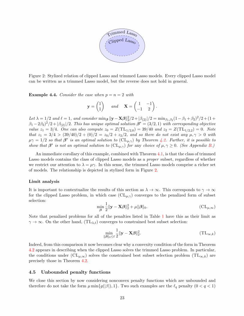
Figure 2: Stylized relation of clipped Lasso and trimmed Lasso models. Every clipped Lasso modelcan be written as a trimmed Lasso model, but the reverse does not hold in general.
Example 4.4. Consider the case when p = n = 2 with
y =
(11
)and X =
(1 −1−1 2
).
Let λ = 1/2 and ` = 1, and consider minβ ‖y−Xβ‖22/2 + |β(2)|/2 = minβ1,β2(1−β1 +β2)2/2 +(1 +
β1− 2β2)2/2 + |β(2)|/2. This has unique optimal solution β∗ = (3/2, 1) with corresponding objective
value z1 = 3/4. One can also compute z0 = Z(TL1/2,0) = 39/40 and z2 = Z(TL1/2,2) = 0. Notethat z1 = 3/4 > (39/40)/2 + (0)/2 = z0/2 + z2/2, and so there do not exist any µ, γ > 0 withµγ = 1/2 so that β∗ is an optimal solution to (CLµ,γ) by Theorem 4.2. Further, it is possible toshow that β∗ is not an optimal solution to (CLµ,γ) for any choice of µ, γ ≥ 0. (See Appendix B.)
An immediate corollary of this example, combined with Theorem 4.1, is that the class of trimmedLasso models contains the class of clipped Lasso models as a proper subset, regardless of whetherwe restrict our attention to λ = µγ. In this sense, the trimmed Lasso models comprise a richer setof models. The relationship is depicted in stylized form in Figure 2.
Limit analysis
It is important to contextualize the results of this section as λ→∞. This corresponds to γ →∞for the clipped Lasso problem, in which case (CLµ,γ) converges to the penalized form of subsetselection:
minβ
1
2‖y −Xβ‖22 + µ‖β‖0. (CLµ,∞)
Note that penalized problems for all of the penalties listed in Table 1 have this as their limit asγ →∞. On the other hand, (TLλ,`) converges to constrained best subset selection:
min‖β‖0≤`
1
2‖y −Xβ‖22. (TL∞,k)
Indeed, from this comparison it now becomes clear why a convexity condition of the form in Theorem4.2 appears in describing when the clipped Lasso solves the trimmed Lasso problem. In particular,the conditions under (CLµ,∞) solves the constrained best subset selection problem (TL∞,k) areprecisely those in Theorem 4.2.
4.5 Unbounded penalty functions
We close this section by now considering nonconvex penalty functions which are unbounded andtherefore do not take the form µmin{g(|β|), 1}. Two such examples are the `q penalty (0 < q < 1)
23
and the log family of penalties as shown in Table 1 and depicted in Figure 1b. Estimation problemswith these penalties can be cast in the form
minφ
1
2‖y −Xφ‖22 + µ
p∑i=1
g(|φi|; γ) (34)
where µ, γ > 0 are parameters, g is an unbounded and strictly increasing function, and g(|φi|; γ)γ→∞−−−→
I{|φi| > 0}. The change of variables in (34) is intentional and its purpose will become clear shortly.Observe that because g is now unbounded, there exists some λ = λ(y,X, µ, γ) > 0 so that for
all λ > λ any optimal solution (φ∗, ε∗) to the problem
minφ,ε
1
2‖y −X(φ + ε)‖22 + λ‖ε‖1 + µ
p∑i=1
g(|φi|; γ) (35)
has ε∗ = 0.11 Therefore, (34) is a special case of (35). We claim that in the limit as γ → ∞ (allelse fixed), that (35) can be written exactly as a trimmed Lasso problem (TLλ,k) for some choiceof k and with the identification of variables β = φ + ε.
We summarize this as follows:
Proposition 4.5. As γ →∞, the penalized estimation problem (34) is a special case of the trimmedLasso problem.
Proof. This can be shown in a straightforward manner: namely, as γ →∞, (35) becomes
minφ,ε
1
2‖y −X(φ + ε)‖22 + λ‖ε‖1 + µ‖φ‖0
which can be in turn written as
minφ,ε:‖φ‖0≤k
1
2‖y −X(φ + ε)‖22 + λ‖ε‖1
for some k ∈ {0, 1, . . . , p}. But as per the observations of Section 2.3, this is exactly (TLλ,k) usinga change of variables β = φ+ ε. In the case when λ is sufficiently large, we necessarily have β = φat optimality.
While this result is not surprising (given that as γ →∞ the problem is (34) is precisely penalizedbest subset selection), it is useful for illustrating the connection between (34) and the trimmedLasso problem even when the trimmed Lasso parameter λ is not necessarily large: in particular,(TLλ,k) can be viewed as estimating β as the sum of two components—a sparse component φand small-norm (“noise”) component ε. Indeed, in this setup, λ precisely controls the desirablelevel of allowed “noise” in β. From this intuitive perspective, it becomes clearer why the trimmedLasso type approach represents a continuous connection between best subset selection (λ large)and ordinary least squares (λ small).
We close this section by making the following observation regarding problem (35). In particular,observe that regardless of λ, we can rewrite this as
minβ
1
2‖y −Xβ‖22 +
p∑i=1
ρ(|βi|)
11The proof involves a straightforward modification of an argument along the lines of that given in Theorem 2.3.Also note that we can choose λ so that it is decreasing in γ, ceteris paribus.
24

where ρ(|βi|) is the new penalty function defined as
ρ(|βi|) = minφ+ε=βi
λ|ε|+ µg(|φ|; γ).
For the unbounded and concave penalty functions shown in Table 1, this new penalty functionis quasi-concave and can be rewritten easily in closed form. For example, for the `q penaltyρ(|βi|) = µ|βi|1/γ (where γ > 1), the new penalty function is
ρ(|βi|) = min{µ|βi|1/γ , λ|βi|}.
5 Algorithmic Approaches
We now turn our attention to algorithms for estimation with the trimmed Lasso penalty. Ourprinciple focus throughout will be the same problem considered in Theorem 2.3, namely
minβ
1
2‖y −Xβ‖22 + λTk (β) + η‖β‖1 (36)
We present three possible approaches to finding potential solutions to (36): a first-order-basedalternating minimization scheme that has accompanying local optimality guarantees and was firststudied in [39, 72]; an augmented Lagrangian approach that appears to perform noticeably better,despite lacking optimality guarantees; and a convex envelope approach. We contrast these methodswith approaches for certifying global optimality of solutions to (36) (described in [69]) and includean illustrative computational example. Implementations of the various algorithms presented canbe found at
https://github.com/copenhaver/trimmedlasso.
5.1 Upper bounds via convex methods
We start by focusing on the application of convex optimization methods to finding to findingpotential solutions to (36). Technical details are contained in Appendix C.
Alternating minimization scheme
We begin with a first-order-based approach for obtaining a locally optimal solution of (36) asdescribed in [39,72]. The key tool in this approach is the theory of difference of convex optimization(“DCO”) [1, 2, 66]. Set the following notation:
f(β) = ‖y −Xβ‖22/2 + λTk (β) + η‖β‖1,f1(β) = ‖y −Xβ‖22/2 + (η + λ)‖β‖1,f2(β) = λ
∑ki=1 |β(i)|.
Let us make a few simple observations:
(a) Problem (36) can be written as minβf(β).
(b) For all β, f(β) = f1(β)− f2(β).
(c) The functions f1 and f2 are convex.
25
While simple, these observations enable one to apply the theory of DCO, which focuses preciselyon problems of the form
minβf1(β)− f2(β),
where f1 and f2 are convex. In particular, the optimality conditions for such a problem havebeen studied extensively [2]. Let us note that while it may appear that the representation of theobjective f as f1 − f2 might otherwise seem like an artificial algebraic manipulation, the min-min representation in Theorem 3.1 shows how such a difference-of-convex representation can arisenaturally.
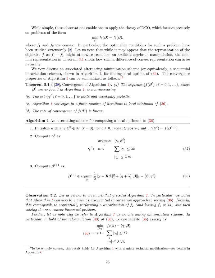
We now discuss an associated alternating minimization scheme (or equivalently, a sequentiallinearization scheme), shown in Algorithm 1, for finding local optima of (36). The convergenceproperties of Algorithm 1 can be summarized as follows:12
Theorem 5.1 ( [39], Convergence of Algorithm 1). (a) The sequence {f(β`) : ` = 0, 1, . . .}, whereβ` are as found in Algorithm 1, is non-increasing.
(b) The set {γ` : ` = 0, 1, . . .} is finite and eventually periodic.
(c) Algorithm 1 converges in a finite number of iterations to local minimum of (36).
(d) The rate of convergence of f(β`) is linear.
Algorithm 1 An alternating scheme for computing a local optimum to (36)
1. Initialize with any β0 ∈ Rp (` = 0); for ` ≥ 0, repeat Steps 2-3 until f(β`) = f(β`+1).
2. Compute γ` as
γ` ∈
argmaxγ
〈γ,β`〉
s. t.∑i
|γi| ≤ λk
|γi| ≤ λ ∀i.
(37)
3. Compute β`+1 as
β`+1 ∈ argminβ
1
2‖y −Xβ‖22 + (η + λ)‖β‖1 − 〈β,γ`〉. (38)
Observation 5.2. Let us return to a remark that preceded Algorithm 1. In particular, we notedthat Algorithm 1 can also be viewed as a sequential linearization approach to solving (36). Namely,this corresponds to sequentially performing a linearization of f2 (and leaving f1 as is), and thensolving the new convex linearized problem.
Further, let us note why we refer to Algorithm 1 as an alternating minimization scheme. Inparticular, in light of the reformulation (43) of (36), we can rewrite (36) exactly as
(36) =
minβ,γ
f1(β)− 〈γ,β〉
s. t.∑i
|γi| ≤ λk
|γi| ≤ λ ∀i.12To be entirely correct, this result holds for Algorithm 1 with a minor technical modification—see details in
Appendix C.
26

In this sense, if one takes care in performing alternating minimization in β (with γ fixed) and inγ (with β fixed) (as in Algorithm 1), then a locally optimal solution is guaranteed.
We now turn to how to actually apply Algorithm 1. Observe that the algorithm is quite simple;in particular, it only requires solving two types of well-structured convex optimization problems.The first such problem, for a fixed β, is shown in (37). This can be solved in closed form by simplysorting the entries of |β|, i.e., by finding |β(1)|, . . . , |β(p)|. The second subproblem, shown in (38) fora fixed γ, is precisely the usual Lasso problem and is amenable to any of the possible algorithmsfor the Lasso [31,42,70].
Augmented Lagrangian approach
We briefly mention another technique for finding potential solutions to (36) using an AlternatingDirections Method of Multiplers (ADMM) [20] approach. To our knowledge, the application ofADMM to the trimmed Lasso problem is novel, although it appears closely related to [68]. Webegin by observing that (36) can be written exactly as
minβ,γ
12 ‖y −Xβ‖22 + η ‖β‖1 + λTk (γ)
s. t. β = γ,
which makes use of the canonical variable splitting. Introducing dual variable q ∈ Rp and parameterσ > 0, this becomes in augmented Lagrangian form
minβ,γ
maxq
1
2‖y −Xβ‖22 + η ‖β‖1 + λTk (γ) +
〈q,β − γ〉+σ
2‖β − γ‖22 . (39)
The utility of such a reformulation is that it is directly amenable to ADMM, as detailed inAlgorithm 2. While the problem is nonconvex and therefore the ADMM is not guaranteed toconverge, numerical experiments suggest that this approach has superior performance to the DCO-inspired method considered in Algorithm 1.
We close by commenting on the subproblems that must be solved in Algorithm 2. Step 2 canbe carried out using “hot” starts. Step 3 is the solution of the trimmed Lasso in the orthogonaldesign case and can be solved by performed by sorting p numbers; see Appendix C.
Convexification approach
We briefly consider the convex relaxation of the problem (36). We begin by computing the convexenvelope [21,60] of Tk on [−1, 1]p (here the choice of [−1, 1]p is standard, such as in the convexifica-tion of `0 over this set which leads to `1). The proof follows standard techniques (e.g. computingthe biconjugate [60]) and is omitted.
Lemma 5.3. The convex envelope of Tk on [−1, 1]p is the function Tk defined as
Tk(β) = (‖β‖1 − k)+ .
In words, the convex envelope of Tk is a “soft thresholded” version of the Lasso penalty (thresh-olded at level k). This can be thought of as an alternative way of interpreting the name “trimmedLasso.”
27
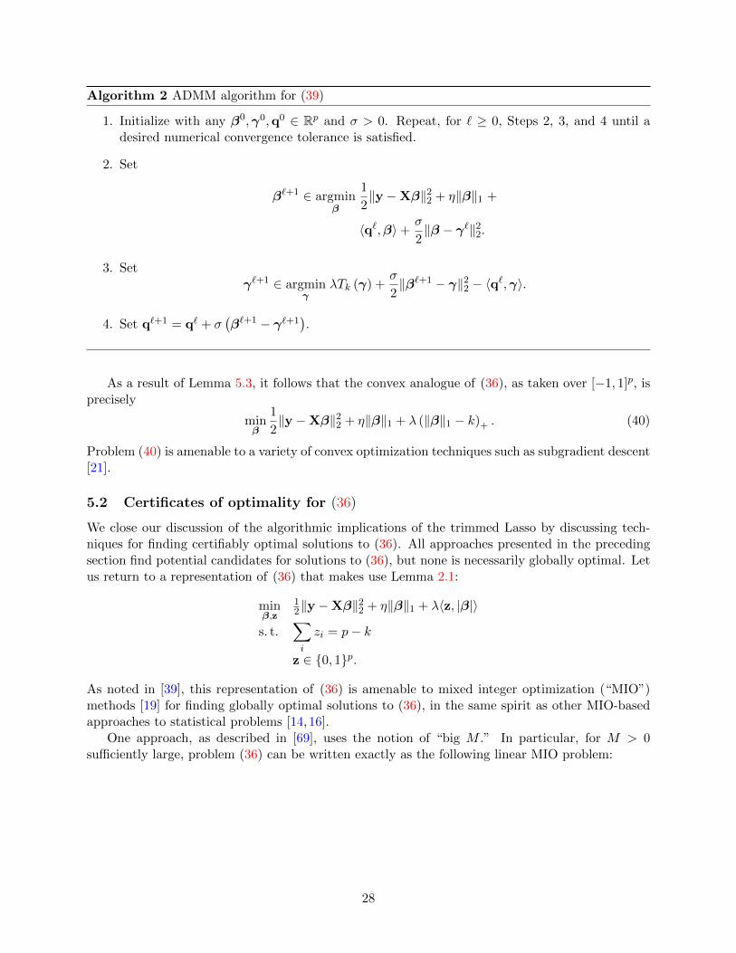
Algorithm 2 ADMM algorithm for (39)
1. Initialize with any β0,γ0,q0 ∈ Rp and σ > 0. Repeat, for ` ≥ 0, Steps 2, 3, and 4 until adesired numerical convergence tolerance is satisfied.
2. Set
β`+1 ∈ argminβ
1
2‖y −Xβ‖22 + η‖β‖1 +
〈q`,β〉+σ
2‖β − γ`‖22.
3. Setγ`+1 ∈ argmin
γλTk (γ) +
σ
2‖β`+1 − γ‖22 − 〈q`,γ〉.
4. Set q`+1 = q` + σ(β`+1 − γ`+1
).
As a result of Lemma 5.3, it follows that the convex analogue of (36), as taken over [−1, 1]p, isprecisely
minβ
1
2‖y −Xβ‖22 + η‖β‖1 + λ (‖β‖1 − k)+ . (40)
Problem (40) is amenable to a variety of convex optimization techniques such as subgradient descent[21].
5.2 Certificates of optimality for (36)
We close our discussion of the algorithmic implications of the trimmed Lasso by discussing tech-niques for finding certifiably optimal solutions to (36). All approaches presented in the precedingsection find potential candidates for solutions to (36), but none is necessarily globally optimal. Letus return to a representation of (36) that makes use Lemma 2.1:
minβ,z
12‖y −Xβ‖22 + η‖β‖1 + λ〈z, |β|〉
s. t.∑i
zi = p− k
z ∈ {0, 1}p.
As noted in [39], this representation of (36) is amenable to mixed integer optimization (“MIO”)methods [19] for finding globally optimal solutions to (36), in the same spirit as other MIO-basedapproaches to statistical problems [14,16].
One approach, as described in [69], uses the notion of “big M .” In particular, for M > 0sufficiently large, problem (36) can be written exactly as the following linear MIO problem:
28

minβ,z,a
1
2‖y −Xβ‖22 + η‖β‖1 + λ
∑i
ai
s. t.∑i
zi = p− k
z ∈ {0, 1}pa ≥ β +Mz−M1a ≥ −β +Mz−M1a ≥ 0.
(41)
This representation as a linear MIO problem enables the direct application of numerous existingMIO algorithms (such as [40]).13 Also, let us note that the linear relaxation of (41), i.e., problem(41) with the constraint z ∈ {0, 1}p replaced with z ∈ [0, 1]p, is the problem
minβ
1
2‖y −Xβ‖22 + η‖β‖1 + λ (‖β‖1 −Mk)+ ,
where we see the convex envelope penalty appear directly. As such, when M is large, the linearrelaxation of (41) is the ordinary Lasso problem minβ
12‖y −Xβ‖22 + η‖β‖1.
5.3 Computational example
Because a rigorous computational comparison is not the primary focus of this paper, we provide alimited demonstration that describes the behavior of solutions to (36) as computed via the differentapproaches. Precise computational details are contained in Appendix C.4. We will focus on twodifferent aspects: sparsity and approximation quality.
Sparsity properties
As the motivation for the trimmed Lasso is ostensibly sparse modeling, its sparsity properties areof particular interest. We consider a problem instance with p = 20, n = 100, k = 2, and signal-to-noise ratio 10 (the sparsity of the ground truth model βtrue is 10). The relevant coefficient profilesas a function of λ are shown in Figure 3. In this example none of the convex approaches finds theoptimal two variable solution computed using mixed integer optimization. Further, as one wouldexpect a priori, the optimal coefficient profiles (as well as the ADMM profiles) are not continuousin λ. Finally, note that by design of the algorithms, the alternating minimization and ADMMapproaches yield solutions with sparsity at most k for λ sufficiently large.
Optimality gap
Another critical question is the degree of suboptimality of solutions found via the convex approaches.We average optimality gaps across 100 problem instances with p = 20, n = 100, and k = 2; therelevant results are shown in Figure 4. The results are entirely as one might expect. When λ issmall and the problem is convex or nearly convex, the heuristics perform well. However, this breaksdown as λ increases and the sparsity-inducing nature of the trimmed Lasso penalty comes into play.Further, we see that the convex envelope approach tends to perform the worst, with the ADMM
13There are certainly other possible representations of (43), such as using special ordered set (SOS) constraints,see e.g. [14]. Without more sophisticated tuning of M as in [14], the SOS formulations appear to be vastly superiorin terms of time required to prove optimality. The precise formulation essentially takes the form of problem (10). AnSOS-based implementation is provided in the supplementary code as the default method of certifying optimality.
29

Alternating M
inimization
AD
MM
Convex E
nvelope
0 1 2 3 4 5
−5
0
5
−5
0
5
−5
0
5
λ
Coe
ffici
ent V
alue
s
Heuristic shown in solid black; optimal shown in dashed blue
Regularization paths for heuristic algorithms, as compared with optimal
Figure 3
30

0%
3%
6%
9%
12%
0 2 4 6λ
Rel
ativ
e op
timal
ity g
ap (
%)
AlgorithmAlternating MinimizationADMMConvex EnvelopeMIO (Optimal)
Relative optimality gaps for heuristic algorithms
Figure 4
performing the best of the three heuristics. This is perhaps not surprising, as any solution foundvia the ADMM can be guaranteed to be locally optimal by subsequently applying the alternatingminimization scheme of Algorithm 1 to any solution found via Algorithm 2.
Computational burden
Loosely speaking, the heuristic approaches all carry a similar computational cost per iteration,namely, solving a Lasso-like problem. In contrast, the MIO approach can take significantly morecomputational resources. However, by design, the MIO approach maintains a suboptimality gapthroughout computation and can therefore be terminated, before optimality is certified, with acertificate of suboptimality. We do not consider any empirical analysis of runtime here.
Other considerations
There are other additional computational considerations that are potentially of interest as well,but they are primarily beyond the scope of the present work. For example, instead of consideringoptimality purely in terms of objective values in (36), there are other critical notions from a sta-tistical perspective (e.g. ability to recover true sparse models and performance on out-of-sampledata) that would also be necessary to consider across the multiple approaches.
6 Conclusions
In this work, we have studied the trimmed Lasso, a nonconvex adaptation of Lasso that acts as anexact penalty method for best subset selection. Unlike some other approaches to exact penalizationwhich use coordinate-wise separable functions, the trimmed Lasso offers direct control of the desiredsparsity k. Further, we emphasized the interpretation of the trimmed Lasso from the perspective
31
of robustness. In doing so, we provided contrasts with the SLOPE penalty as well as comparisonswith estimators from the robust statistics and total least squares literature.
We have also taken care to contextualize the trimmed Lasso within the literature on nonconvexpenalized estimation approaches to sparse modeling, showing that penalties like the trimmed Lassocan be viewed as a generalization of such approaches in the case when the penalty function isbounded. In doing so, we also highlighted how precisely the problems were related, with a completecharacterization given in the case of the clipped Lasso.
Finally, we have shown how modern developments in optimization can be brought to bear forthe trimmed Lasso to create convex optimization optimization algorithms that can take advantageof the significant developments in algorithms for Lasso-like problems in recent years.
Our work here raises many interesting questions about further properties of the trimmed Lassoand the application of similar ideas in other settings. We see two particularly noteworthy directionsof focus: algorithms and statistical properties. For the former, we anticipate that an approach liketrimmed Lasso, which leads to relatively straightforward algorithms that use close analogues fromconvex optimization, is simple to interpret and to implement. At the same time, the heuristicapproaches to the trimmed Lasso presented herein carry no more of a computational burden thansolving convex, Lasso-like problems. On the latter front, we anticipate that a deeper analysis of thestatistical properties of estimators attained using the trimmed Lasso would help to illuminate itin its own right while also further connecting it to existing approaches in the statistical estimationliterature.
Appendix A General min-max representation of SLOPE
For completeness, in this appendix we include the more general representation of the SLOPEpenalty RSLOPE(w) in the same spirit of Proposition 1.2. Here we work with SLOPE in its mostgeneral form, namely,
RSLOPE(w)(β) =
p∑i=1
wi|β(i)|,
where w is a (fixed) vector of weights with w1 ≥ w2 ≥ · · · ≥ wp ≥ 0 and w1 > 0.To describe the general min-max representation, we first set some notation. For a matrix
∆ ∈ Rn×p, we let ν(∆) ∈ Rp be the vector (‖∆1‖2, . . . , ‖∆p‖2) with entries sorted so that ν1 ≥ν2 ≥ · · · ≥ νp. As usual, for two vectors x and y, we use x ≤ y to denote that coordinate-wiseinequality holds. With this notation, we have the following:
Proposition A.1. Problem (9) with uncertainty set
Uw = {∆ : ν(∆) ≤ w}
is equivalent to problem (3) with R(β) = RSLOPE(w)(β). Further, problem (9) with uncertainty set
Uw ={∆ : ‖∆φ‖2 ≤ RSLOPE(w)(φ) ∀φ
}is equivalent to problem (3) with R(β) = RSLOPE(w)(β).
The proof, like the proof of Proposition 1.2, follows basic techniques described in [9] and istherefore omitted.
32

Appendix B Additional proofs
This appendix section contains supplemental proofs not contained in the main text.
Proof of Theorem 2.3. Let λ = ‖y‖2 · (maxj ‖xj‖2), where xj denotes the jth row of X. We fixλ > λ, k, and η > 0 throughout the entire proof. We begin by observing that it suffices to showthat any solution β to
minβ
1
2‖y −Xβ‖22 + λTk (β) + η‖β‖1 (42)
satisfies Tk (β) = 0, or equivalently, ‖β‖0 ≤ k. As per Lemma 2.1, problem (42) can be rewrittenexactly as
minβ,z
12‖y −Xβ‖22 + λ〈z, |β|〉+ η‖β‖1
s. t.∑i
zi = p− k
z ∈ {0, 1}p.
(43)
Let (β∗, z∗) be any solution to (43). Observe that necessarily β∗ is also a solution to the problem
minβ
1
2‖y −Xβ‖22 + λ〈z∗, |β|〉+ η‖β‖1. (44)
Note that, unlike (42), the problem in (44) is readily amenable to an analysis using the theory ofproximal gradient methods [7, 28]. In particular, we must have for any γ > 0 that
β∗ = proxγR(β∗ − γ(X′Xβ∗ −X′y)
), (45)
where R(β) = η‖β‖1 + λ∑
i : z∗i =1
|βi|. Suppose that Tk (β∗) > 0. In particular, for some j ∈
{1, . . . , p}, we have β∗j 6= 0 and z∗j = 1. Yet, as per (45),14∣∣β∗j − γ〈xj ,Xβ∗ − y〉∣∣ > γ(η + λ) for all γ > 0,
where xj denotes the jth row of X. This implies that
|〈xj ,Xβ∗ − y〉| ≥ η + λ.
Now, using the definition of λ, observe that
η + λ ≤ |〈xj ,Xβ∗ − y〉| ≤ ‖xj‖2‖Xβ∗ − y‖2≤ ‖xj‖2‖y‖ ≤ λ < λ,
which is a contradiction since η > 0. Hence, Tk (β∗) = 0, completing the proof.
14This is valid for the following reason: since β∗j 6= 0 and β∗j satisfies (45), it must be the case that∣∣β∗j − γx′j(Xβ∗ − y)∣∣ > γ(η+λ), for otherwise the soft-thresholding operator at level γ(η+λ) would set this quantity
to zero.
33

Extended statement of Proposition 2.5
We now include a precise version of the convergence claim in Proposition 2.5. Let us set a standardnotion: we say that β is ε-optimal (for ε > 0) to an optimization problem (P) if the optimalobjective value of (P) is within ε of the objective value of β. We add an additional regularizerη‖β‖1, for η > 0 fixed, to the objective in order to ensure coercivity of the objective functions.
Proposition B.1 (Extended form of Proposition 2.5). Let g : R+ → R+ be an unbounded, contin-uous, and strictly increasing function with g(0) = 0. Consider the problems
minβ
1
2‖y −Xβ‖22 + λπgk(β) + η‖β‖1 (46)
and
min‖β‖0≤k
1
2‖y −Xβ‖22 + η‖β‖1. (47)
For every ε > 0, there exists some λ = λ(ε) > 0 so that for all λ > λ,
1. For every optimal β∗ to (46), there is some β so that ‖β∗ − β‖2 ≤ ε, β is feasible to (47),and β is ε-optimal to (47).
2. Every optimal β∗ to (47) is ε-optimal to (46).
Proof. The proof follows a basic continuity argument that is simpler than the one presented belowin Theorem B.2. For that reason, we do not include a full proof. Observe that the assumptionson g imply that g−1 is well-defined on, say, g([0, 1]). If we let ε > 0 and suppose that β∗ isoptimal to (46), where λ > λ := ‖y‖22/(2g(ε/p)), and if we define β to be β∗ with all but the klargest magnitude entries truncated to zero (ties broken arbitrarily), then πgk(β∗) ≤ ‖y‖22/(2λ) and
πgk(β∗) =∑p
i=1 g(|β∗i − βi|) so that |β∗i − βi| ≤ g−1(‖y‖22/(2λ)) ≤ ε/p by definition of λ. Hence,
‖β∗ − β‖1 ≤ ε, and all the other claims essentially follow from this.
Proof of Theorem 3.1. We begin by showing that for any β,
min∆∈Uλk
‖y − (X + ∆)β‖2 =
(‖y −Xβ‖2 − λ
k∑i=1
|β(i)|
)+
where (a)+ := max{0, a}. Fix β and set r = y −Xβ. We assume without loss of generality thatr 6= 0 and that β 6= 0. For any ∆, note that ‖r−∆β‖2 ≥ 0 and ‖r−∆β‖2 ≥ ‖r‖2 − ‖∆β‖2 bythe reverse triangle inequality. Now observe that for ∆ ∈ Uλk ,
‖∆β‖2 ≤∑i
|βi|‖∆i‖2 ≤k∑i=1
λ|β(i)|.
Therefore, ‖r −∆β‖2 ≥(‖r‖2 − λ
∑ki=1 |β(i)|
)+
. Let I ⊆ {1, . . . , p} be a set of k indices which
correspond to the k largest entries of β (if |β(k)| = |β(k+1)|, break ties arbitrarily). Define ∆ ∈ Uλkas the matrix whose ith column is {
λ sgn(βi)r/‖r‖2, i ∈ I0, i /∈ I,
34

where λ = min{λ, ‖r‖2/
(∑ki=1 |β(i)|
)}. It is easy to verify that ∆ ∈ Uλk and ‖r − ∆β‖2 =(
‖r‖2 − λ∑k
i=1 |β(i)|)+
. Combined with the lower bound, we have
min∆∈Uλk
‖y − (X + ∆)β‖2 =
(‖y −Xβ‖2 − λ
k∑i=1
|β(i)|
)+
which completes the first claim.It follows that the problem (20) can be rewritten exactly as
minβ
(‖y −Xβ‖2 − λ
k∑i=1
|β(i)|
)+
+ r(β). (48)
To finish the proof of the theorem, it suffices to show that if β∗ is a solution to (48), then
‖y −Xβ∗‖2 − λk∑i=1
|β∗(i)| ≥ 0.
If this is not true, then ‖y −Xβ∗‖2 − λ∑k
i=1 |β∗(i)| < 0 and so β∗ 6= 0. However, this implies that
for 1 > ε > 0 sufficiently small, βε := (1− ε)β∗ satisfies ‖y−Xβε‖2 − λ∑k
i=1 |(βε)(i)| < 0. This inturn implies that (
‖y −Xβε‖2 − λ∑k
i=1 |(βε)(i)|)+
+ r(βε)
<(‖y −Xβ∗‖2 − λ
∑ki=1 |β∗(i)|
)+
+ r(β∗),
which contradicts the optimality of β∗. (We have used the absolute homogeneity of the norm r andthat β∗ 6= 0.) Hence, any optimal β∗ to (48) necessarily satisfies ‖y −Xβ∗‖2 − λ
∑ki=1 |β∗(i)| ≥ 0
and so the desired results follows.
N.B. The assumption that r is a norm can be relaxed somewhat (as is clear in the proof),although the full generality is not necessary for our purposes.
Corollary 3.2 and related discussions
Here we include a precise statement of the “approximate” claim in Corollary 3.2. After the proof,we include a discussion of related technical issues.
Theorem B.2 (Precise statement of Corollary 3.2). For τ > λ > 0, consider the problems
minβ
‖y −Xβ‖2 + (τ − λ)‖β‖1 + λTk (β)
s. t. λk∑i=1
|β(i)| ≤ ‖y −Xβ‖2.(49)
andminβ‖y −Xβ‖2 + (τ − λ)‖β‖1 + λTk (β) . (50)
For all ε > 0, there exists λ = λ(ε) > 0 so that whenever λ ∈ (0, λ),
1. Every optimal β∗ to (49) is ε-optimal to (50).
35

2. For every optimal β∗ to (50), there is some β so that ‖β∗ − β‖2 ≤ ε, β is feasible to (49),and β is ε-optimal to (49).
Proof. Fix τ > 0 throughout. We assume without loss of generality that y 6= 0, as otherwise theclaim is obvious. We will prove the second claim first, as it essentially implies the first.
Let us consider two situations. In particular, we consider whether there exists a nonzero optimalsolution to
minβ‖y −Xβ‖2 + τ‖β‖1. (51)
Case 1—existence of nonzero optimal solution to (51)
We first consider the case when there exists a nonzero solution to problem (51). We show a fewlemmata:
1. We first show that the norm of solutions to (50) are uniformly bounded away from zero,independent of λ. To proceed, let β be any nonzero optimal solution to (51). Observe thatif β∗ is optimal to (50), then
‖y −Xβ∗‖2 + (τ − λ)‖β∗‖1 + λTk(β∗) ≤ ‖y −Xβ‖2 + (τ − λ)‖β‖1 + λTk(β)
≤ ‖y −Xβ∗‖2 + τ‖β∗‖1 − λ‖β‖1 + λTk(β),
implying that ‖β‖1 − Tk(β) ≤ ‖β∗‖1 − Tk(β∗). In other words,∑k
i=1 |β(i)| ≤∑k
i=1 |β∗(i)| ≤‖β∗‖1. Using the fact that β 6= 0, we have that any solution β∗ to (50) has strictly positivenorm:
‖β∗‖1 ≥ C > 0,
where C :=∑k
i=1 |β(i)| is a universal constant depending only on τ (and not λ).
2. We now upper bound the norm of solutions to (50). In particular, if β∗ is optimal to (50),then
‖y −Xβ∗‖2 + (τ − λ)‖β∗‖1 + λTk(β∗) ≤ ‖y‖2 + 0 + 0 = ‖y‖2,
and so ‖β∗‖1 ≤ ‖y‖2/(τ−λ). (This bound is not uniform in λ, but if we restrict our attentionto, say λ ≤ τ/2, it is.)
3. We now lower bound the loss for scaled version of optimal solutions. In particular, if σ ∈ [0, 1]and β∗ is optimal to (50), then by optimality we have that
‖y −Xβ∗‖2 + (τ − λ)‖β∗‖1 + λTk(β∗) ≤ ‖y − σXβ∗‖2 + (τ − λ)σ‖β∗‖1 + λσTk(β
∗),
which in turn implies that
‖y − σXβ∗‖2 ≥ ‖y −Xβ∗‖2 + (τ − λ)(1− σ)‖β∗‖1 + λ(1− σ)Tk(β∗)
≥ ‖y −Xβ∗‖2 + (τ − λ)(1− σ)C ≥ (τ − λ)(1− σ)C
by combining with the first observation.
Using these, we are now ready to proceed. Let ε > 0; we assume without loss of generality thatε < 2‖y‖2/τ . Let
λ := min
{ετ3C
4‖y‖2(2‖y‖2 − ετ),τ
2
}.
36

Fix λ ∈ (0, λ) and let β∗ be any optimal solution to (50). Define
σ :=
(1− ετ
2‖y‖2
)and β := σβ∗.
We claim that β satisfies the desired requirements of the theorem:
1. We first argue that ‖β∗ − β‖2 ≤ ε. Observe that
‖β∗ − β‖2 = ετ‖β∗‖2/(2‖y‖2) ≤ ετ‖β∗‖1/(2‖y‖2) ≤ ετ‖y‖2/(2‖y‖2(τ − λ)) ≤ ε.
2. We now show that β is feasible to (49). This requires us to argue that λ∑k
i=1 |β(i)| ≤‖y −Xβ‖2. Yet,
λk∑i=1
|β(i)| ≤ λ‖β‖1 = λσ‖β∗‖1 ≤ 2λσ‖y‖2/τ ≤τ
2(1− σ)C
≤ (τ − λ)(1− σ)C ≤ ‖y − σXβ∗‖2 = ‖y −Xβ‖2,
as desired. The only non-obvious step is the inequality 2λσ‖y‖2/τ ≤ τ(1 − σ)C/2, whichfollows from algebraic manipulations using the definitions of σ and λ.
3. Finally, we show that β is (ε‖X‖2)-optimal to (49). Indeed, because β∗ is optimal to (50)which necessarily lowers bound problem (49), we have that the objective value gap betweenβ and an optimal solution to (49) is at most
‖y − σXβ∗‖2 − ‖y −Xβ∗‖2 + (τ − λ)(σ − 1)‖β∗‖1 + λ(σ − 1)Tk(β∗)
≤ (1− σ)‖Xβ∗‖2 + 0 + 0 ≤ (1− σ)‖X‖2‖β∗‖2 ≤ 2(1− σ)‖X‖2‖y‖2/τ= 2ετ/(2‖y‖2)‖X‖2‖y‖2/τ = ε‖X‖2.
As the choice of ε > 0 was arbitrary, this completes the proof of claim 2 in the theorem in the casewhen 0 is not a solution to (51).
Case 2—no nonzero optimal solution to (51)
In the case when there is no nonzero optimal solution to (51), 0 is optimal and it is the only optimalpoint. Our analysis will be similar to the previous approach, with the key difference being in howwe lower bound the quantity ‖y − σXβ∗‖2 where β∗ is optimal to (50). Again, we have severallemmata:
1. As before, if β∗ is optimal to (50), then ‖β∗‖1 ≤ ‖y‖2/(τ − λ).
2. We now lower bound the quantity ‖y − σXβ∗‖2, where β∗ is optimal to (50) and σ ∈ [0, 1].As such, consider the function
f(σ) := ‖y − σXβ∗‖2 + στ‖β∗‖1.
Because f is convex in σ and the unique optimal solution to (51) is 0, we have that
f(σ) ≥ f(0) + σf ′(0) ∀σ ∈ [0, 1] and f ′(0) ≥ 0
37

(It is not difficult to argue that f is differentiable at 0.) An elementary computation showsthat f ′(0) = τ‖β∗‖1 − 〈y,Xβ∗〉/‖y‖2. Therefore, we have that
‖y − σXβ∗‖2 + στ‖β∗‖1 ≥ ‖y‖2 + σ (τ‖β∗‖1 − 〈y,Xβ∗〉/‖y‖2) ,
implying that
‖y − σXβ∗‖2 ≥ ‖y‖2 − σ〈y,Xβ∗〉/‖y‖2 ≥ ‖y‖2 − στ‖β∗‖1 ≥ ‖y‖2 − στ‖y‖2/(τ − λ),
with the final step following by an application of the previous lemma.
We are now ready to proceed. Let ε > 0; we assume without loss of generality that ε < 2‖y‖2/τ .Let
λ := min
{ετ2
4‖y‖2 − ετ,τ
2
}.
Fix λ ∈ (0, λ) and let β∗ be any optimal solution to (50). Define
σ :=
(1− ετ
2‖y‖2
)and β := σβ∗.
We claim that β satisfies the desired requirements:
1. The proof of the claim that ‖β∗ − β‖2 ≤ ε is exactly as before.
2. We now show that β is feasible to (49), which requires a different proof. Again this requiresus to argue that λ
∑ki=1 |β(i)| ≤ ‖y −Xβ‖2. Yet,
λk∑i=1
|β(i)| ≤ λ‖β‖1 = λσ‖β∗‖1 ≤ λσ‖y‖2/(τ − λ) ≤ ‖y‖2 − στ‖y‖2/(τ − λ)
≤ ‖y − σXβ∗‖2 = ‖y −Xβ‖2,
as desired. The only non-obvious step is the inequality λσ‖y‖2/(τ−λ) ≤ ‖y‖2−στ‖y‖2/(τ−λ), which follows from algebraic manipulations using the definitions of σ and λ.
3. Finally, the proof that β is (ε‖X‖2)-optimal to (49) follows in the same way as before.
Therefore, we conclude that in the case when 0 is the unique optimal solution to (51), thenagain we have that the claim 2 of the theorem holds.
Finally, we show that claim 1 holds: any solution β∗ to (49) is ε-optimal to (50). This followsby letting β be any optimal solution to (50). By applying the entire argument above, we know thatthe objective value of some β, feasible to (49) and close to β, is within ε of the optimal objectivevalue of (49), i.e., the objective value of β∗, and within ε of the objective value of (50), i.e., theobjective value of β. This completes the proof.
In short, the key complication is that the quantity ‖y −Xβ∗‖2 does not need to be uniformlybounded away from zero for solutions β∗ to problem (50). This is part of the complication ofworking with the homogeneous form of the trimmed Lasso problem. For a concrete example, ifone considers the homogeneous Lasso problem with p = n = 1, y = (1), and X = (1), then thehomogeneous Lasso problem minβ ‖y −Xβ‖2 + η‖β‖1 is
minβ|1− β|+ η|β|.
38

For η ∈ [0, 1], β∗ = 1 is an optimal solution to this problem with corresponding error ‖y−Xβ∗‖ = 0.If we make an assumption about the behavior of ‖y − Xβ∗‖, then we do not need the setup asshown above.
Proof of Proposition 3.3. The proof is entirely analogous to that of Theorems 3.1 and B.2 and istherefore omitted.
Proof of validity of Example 4.4. Let us consider the problem instance where p = n = 2 with
y =
(11
)and X =
(1 −1−1 2
).
Let λ = 1/2 and ` = 1, and consider the problem
minβ‖y −Xβ‖22 + |β(2)| = min
β1,β2(1− β1 + β2)
2 + (1 + β1 − 2β2)2 + |β(2)|. (52)
We have omitted the factor of 1/2 as shown in the actual example in the main text in order toavoid unnecessary complications.
Solving problem (52) and its related counterparts (for ` ∈ {0, 2}) can rely on convex analysisbecause we can simply enumerate all possible scenarios. In particular, the solution to (52) isβ∗ = (3/2, 1) based on an analysis of two related problems:
minβ1,β2
(1− β1 + β2)2 + (1 + β1 − 2β2)
2 + |β1|.
minβ1,β2
(1− β1 + β2)2 + (1 + β1 − 2β2)
2 + |β2|.
(We should be careful to impose the additional constraints |β1| ≤ |β2| and |β1| ≥ |β2|, respectively,although a simple argument shows that these constraints are not required in this example.) Astandard convex analysis using the Lasso (e.g. by directly using subdifferentials) shows that theproblems have respective solutions (1/2, 1/2) and (3/2, 1), with the latter having the better objectivevalue in (52). As such, β∗ is indeed optimal. The solution in the cases of ` ∈ {0, 2} follows a similarlystandard analysis.
It is perhaps more interesting to study the general case where µ, γ ≥ 0. In particular, we willshow that β∗ = (3/2, 1) is not an optimal solution to the clipped Lasso problem
minβ1,β2
(1− β1 + β2)2 + (1 + β1 − 2β2)
2 + µmin{γ|β1|, 1}+ µmin{γ|β2|, 1} (53)
for any choices of µ and γ. While in general such a problem may be difficult to fully analyze, wecan again rely on localized analysis using convex analysis. To proceed, let
f(β1, β2) = (1− β1 + β2)2 + (1 + β1 − 2β2)
2 + µmin{γ|β1|, 1}+ µmin{γ|β2|, 1},
with the parameters µ and γ implicit. We consider the following exhaustive cases:
1. γ > 1 : In this case, f is convex and differentiable in a neighborhood of β∗. Its gradient at
β∗ is ∇f(β∗) = (0,−1), and therefore β∗ is neither locally optimal nor globally optimal toproblem (53).
2. γ < 2/3 : In this case, f is again convex and differentiable in a neighborhood of β∗. Its
gradient at β∗ is ∇f(β∗) = (µγ, µγ − 1). Again, this cannot equal (0, 0) and therefore β∗ isneither locally nor globally optimal to problem (53).
39
3. 2/3 < γ < 1 : In this case, f is again convex and differentiable in a neighborhood of β∗.
Its gradient at β∗ is ∇f(β∗) = (0, µγ − 1). As a necessary condition for local optimality,we must have that µγ = 1, implying that µ > 1. Further, if β∗ is optimal to (53), thenf(β∗) ≤ f(0, 0). Yet,
f(β∗) = 1/2 + µ+ µγ = 3/2 + µ
f(0, 0) = 2,
implying that µ ≤ 1/2, in contradiction of µ > 1. Hence, β∗ cannot be optimal to (53).
4. γ = 2/3 : In this case, we make two comparisons, using the points β∗, (0, 0), and (3, 2):
f(β∗) = 1/2 + µ+ 2µ/3 = 1/2 + 5µ/3
f(0, 0) = 2
f(3, 2) = 2µ.
Assuming optimality of β∗, we have that f(β∗) ≤ f(0, 0), i.e., µ ≤ 9/10; similarly, f(β∗) ≤f(3, 2), i.e., µ ≥ 3/2. Clearly both cannot hold, and so therefore β∗ cannot be optimal.
5. γ = 1 : Finally, we see that f(β∗) ≤ f(3, 2) would imply that 1/2 + 2µ ≤ 2µ, which is
impossible; hence, β∗ is not optimal to (53). (This argument can clearly also be used in thecase when γ > 1, although it is instructive to see the argument given above in that case.)
In any case, we have that β∗ cannot be a solution to the clipped Lasso problem (53). This completesthe proof of validity of Example 4.4.
Appendix C Supplementary details for Algorithms
This appendix contains further details on algorithms as discussed in Section 5. The presentationhere is primarily self-contained. Note that the alternating minimization scheme based on difference-of-convex optimization can be found in [39].
C.1 Alternating minimization scheme
Let us set the following notation:
f(β) = ‖y −Xβ‖22/2 + λTk (β) + η‖β‖1,f1(β) = ‖y −Xβ‖22/2 + (η + λ)‖β‖1,f2(β) = λ
∑ki=1 |β(i)|.
Definition C.1. For any function F : Rp → R and ε ≥ 0, we define the ε-subdifferential of F atβ0 ∈ Rp to be the set ∂εF (β0) defined as
{γ ∈ Rp : F (β)− F (β0) ≥ 〈γ,β − β0〉 − ε ∀ β ∈ Rp} .
In particular, when ε = 0, we refer to ∂0F (β0) as the subdifferential of F at β0, and we will denotethis as ∂F (β0).
Using this definition, we have the following result precisely characterizing local and globaloptima of (36).
40
Theorem C.2. (a) A point β∗ is a local minimum of f if and only if ∂f2(β∗) ⊆ ∂f1(β∗).
(b) A point β∗ is a global minimum of f if and only if ∂εf2(β∗) ⊆ ∂εf1(β∗) for all ε ≥ 0.
Proof. This is a direct application of results in [66, Thm. 1]. Part (b) is immediate. The forwardimplication of part (a) is immediate as well; the converse implication follows by observing that f2is a polyhedral convex function [2, Thm. 1(ii)] (see definition therein).
Let us note that ∂f1 and ∂f2 are both easily computable, and hence, local optimality can beverified given some candidate β∗ per Theorem C.2.15 We now discuss the associated alternatingminimization scheme (or equivalently, as a sequential linearization scheme), shown in Algorithm 1for finding local optima of (36) by making use of Theorem C.2. Through what follows, we makeuse of the standard notion of a conjugate function, defined as follows:
Definition C.3. For any function F : Rp → R, we define its conjugate function F ∗ : Rp → R tobe the function
F ∗(γ) = supβ〈γ,β − F (β)〉.
We will make the following minor technical assumption: in step 2) of Algorithm 1, we assumewithout loss of generality that the γ` so computed satisfies the additional criteria:
1. it is an extreme point of the relevant feasible region,
2. and that if ∂f2(β`) 6⊆ ∂f1(β`), then γ` is chosen such that γ` ∈ ∂f2(β`) \ ∂f1(β`).
Solving (37) with these additional assumptions can nearly be solved in closed form by simply sortingthe entries of |β|, i.e., by finding |β(1)|, . . . , |β(p)|.We must take some care to ensure that the secondwithout loss of generality condition on γ is satisfied. This is straightforward but tedious; the detailsare shown in Appendix C.2.
Using this modification, the convergence properties of Algorithm 1 can be proven as follows:
Proof of Theorem 5.1. This is an application of [66, Thms. 3-5]. The only modification is inrequiring that γ` is chosen so that γ` ∈ ∂f2(β
∗) \ ∂f1(β∗) if β` is not a local minimum of f—see [66, §3.3] for a motivation and justification for such a modification. Finally, the correspondencebetween γ` ∈ ∂f2(β`) and (37), and between β`+1 ∈ ∂f∗1 (γ`) and (38), is clear from an elementaryargument applied to subdifferentials of variational formulations of functions.
C.2 Algorithm 1, Step 2
Here we present the details of solving (37) in Algorithm 1 in a way that ensures that the associatedwithout loss of generality claims hold. In doing so, we also implicitly study how to verify theconditions for local optimality (c.f. Theorem C.2). Throughout, we use the sgn function defined as
sgn(x) =
1, x > 0−1, x < 0
0, x = 0.
15For the specific functions of interest, verifying local optimality of a candidate β∗ can be performed inO(pmin{n, p} + p log p) operations; the first component relates to the computation of X′Xβ∗, while the secondcaptures the sorting of the entries of β∗. See Appendix C.2 for details.
41
For fixed β, the problem of interest is
maxγ
〈β,γ〉
s. t.∑i
|γi| ≤ λk
|γi| ≤ λ ∀i.
We wish to find a maximizer γ for which the following hold:
1. γ is an extreme point of the relevant feasible region,
2. and that if ∂f2(β) 6⊆ ∂f1(β), then γ is such that γ ∈ ∂f2(β) \ ∂f1(β).
As the problem on its own can be solved by sorting the entries of β, the crux of the problem isensuring that 2) holds.
Given the highly structured nature of f1 and f2 in our setup, it is simple, albeit tedious, toensure that such a condition is satisfied. Let I = {i : |βi| = |β(k)|}. If |I| = 1, the optimal solutionis unique, and there is nothing to show. Therefore, we will assume that |I| ≥ 2. We will constructan optimal solution γ which satisfies the desired conditions. First observe that we necessarily musthave that 1) γi = λ sgn(βi) if |βi| > |β(k)| and 2) γi = 0 if |βi| < |β(k)|. We now proceed to definethe rest of the entries of γ. We consider two cases:
1. First consider the case when |β(k)| > 0. We claim that ∂f2(β) 6⊆ ∂f1(β). To do so, we will
inspect the ith entries of ∂f1(β) for i ∈ I; as such, let P ji = {δi : δ ∈ ∂fj(β)} for j ∈ {1, 2}and i ∈ I (a projection). For each i ∈ I, we have using basic convex analysis that P 1
i isa singelton: P 1
i = {〈Xi,Xβ − y〉 + (η + λ) sgn(βi)}, where Xi is the ith column of X. Incontrast, because |I| ≥ 2, the set P 2
i is an interval with strictly positive length for each i ∈ I(it is either [−λ, 0] or [0, λ], depending on whether βi < 0 or βi > 0, respectively). Therefore,∂f2(β) 6⊆ ∂f1(β), as claimed.
Fix an arbitrary j ∈ I. Per the above argument, we must have that 〈Xj ,Xβ − y〉 + (η +λ) sgn(βj) 6= 0 or 〈Xj ,Xβ − y〉+ (η + λ) sgn(βj) 6= λ sgn(βj). In the former case, set γi = 0,while in the latter case we define γi = λ sgn(βi) (if both are true, either choice suffices). It isclear that it is possible to fill in the remaining entries of γi for i ∈ I \ {j} in a straightforwardmanner so that γ ∈ ∂f2(β). Further, by construction, γ /∈ ∂f1(β), as desired.
2. Now consider the case when |β(k)| = 0. Using the preceding argument, we see that P 1i is the
interval [〈Xi,Xβ−y〉− (η+λ), 〈Xi,Xβ−y〉+η+λ] for i ∈ I. In contrast, P 2i is the interval
[−λ, λ] for i ∈ I. If for all i ∈ I one has that P 2i ⊆ P 1
i , then the choice of γi for i ∈ I isobvious: any optimal extreme point γ of the problem will suffice. (Note here that it may ormay not be that ∂f2(β) ⊆ ∂f1(β). This entirely depends on βi for i /∈ I.)
Therefore, we may assume that there exists some j ∈ I so that P 2j 6⊆ P 1
j . (It followsimmediately that ∂f2(β) 6⊆ ∂f1(β).) We must have that 〈Xj ,Xβ − y〉 − (η + λ) > −λor 〈Xj ,Xβ − y〉 + (η + λ) < λ. In the former case, set γi = −λ, while in the latter case wedefine γi = λ (if both are true, either choice suffices). It is clear that it is possible to fill inthe remaining entries of γi for i ∈ I \ {j} in a straightforward manner so that γ ∈ ∂f2(β).By construction, γ /∈ ∂f1(β), as desired.
In either case, we have that one can choose γ ∈ ∂f2(β) so that 1) γ is an extreme pointof the feasible region {γ :
∑i |γi| ≤ λk, |γi| ≤ λ ∀i} and that 2) γ ∈ ∂f2(β) \ ∂f1(β) whenever
42

∂f2(β) 6⊆ ∂f1(β). This concludes the analysis; thus, we have shown the validity (and computationalfeasibility) of the without loss of generality claim present in Algorithm 1. Indeed, per our analysis,Step 2 in Algorithm 1 can be solved in O(pmin{n, p}+p log p) operations (sorting of β in O(p log p)followed by O(p) conditionals and gradient evaluation in O(np)). In reality, if we keep track ofgradients in Step 3, there is no need to recompute gradients in Step 2, and therefore in practiceStep 2 is of the same complexity of sorting a list of p numbers. (We assume that X′y has beencomputed offline and store throughout for simplicity.)
C.3 Algorithm 2, Step 3
Here we show how to solve Step 3 in Algorithm 2, namely, solving the orthogonal design trimmedLasso problem
minγλTk (γ) +
σ
2‖β − γ‖22 − 〈q,γ〉, (54)
where β and q are fixed. This is solvable in closed form. Let α = β − q/σ. First observe that wecan rewrite (54) as
(54) = minγλTk (γ) + σ‖γ −α‖22/2
= minγ,z:∑
i zi=p−kz∈{0,1}p
λ〈z, |γ|〉+ σ‖γ −α‖22/2
= minγ,z:∑
i zi=p−kz∈{0,1}p
∑i
(λzi|γ|+ σ(γi − αi)2/2
).
The penultimate step follows via Lemma 2.1. Per this final representation, the solution becomesclear. In particular, let I be a set of k indices of α corresponding to α(1), α(2), . . . , α(k). (If|α(k)| = |α(k+1)|, we break ties arbitrarily.) Then a solution γ∗ to (54) is
γ∗i =
{αi, i ∈ I
softλ/σ(αi), i /∈ I,
where softλ/σ(αi) = sgn(αi) |αi − λ/σ|.
C.4 Computational details
For completeness and reproducibility, we also include all computational details. For Figure 3, thefollowing parameters were used to generate the test instance: n = 100, p = 20, SNR = 10, juliaseed = 1, η = 0.01, k = 2. The example was generated from the following true model:
1. βtrue is a vector with ten entries equal to 1 and all others equal to zero. (So ‖βtrue‖0 = 10.)
2. covariance matrix Σ is generated with Σij = .8|i−j|.
3. X ∼ N(0,Σ).
4. εii.i.d.∼ N(0,β′0Σβ0/SNR)
5. y is then defined as Xβ0 + ε
43

The 100 examples generated for Figure 4 were using the following parameters: n = 100, p = 20,SNR = 10, julia seed ∈ {1, . . . , 100}, η = 0.01, k = 2, bigM = 20. MIO using Gurobi solver.Max iterations: alternating minimization—1000; ADMM (inner)—2000; ADMM (outer)—10000.ADMM parameters: σ = 1, τ = 0.9. The examples themselves had the same structure as theprevious example. The optimal gaps shown are relative to the objective in (36). The averagesare computed as geometric means (relative to optimal 100%) across the 100 instances, and thendisplayed relative to the optimal 100%.
Acknowledgments
Copenhaver was partially supported by the Department of Defense, Office of Naval Research,through the National Defense Science and Engineering Graduate (NDSEG) Fellowship. Mazumderwas partially supported by ONR Grant N000141512342.
References
[1] L. T. H. An, “Analyse numerique des algorithmes de l’optimisation DC. Approches locale etglobale. Codes et simulations numeriques en grande dimension. Applications,” Ph.D. disserta-tion, Universite de Rouen, 1994.
[2] L. T. H. An and P. D. Tao, “The DC (difference of convex functions) programming andDCA revisited with DC models of real world nonconvex optimization problems,” Annals ofOperations Research, vol. 133, pp. 23–46, 2005.
[3] T. Anderson, An Introduction to Multivariate Statistical Analysis, 3rd ed. Wiley, New York,2003.
[4] R. Andreani, L. Secchin, and P. Silva, “Convergence properties of a second order augmentedLagrangian method for mathematical programs with complementarity constraints,” 2017.
[5] A. Bandeira, E. Dobriban, D. Mixon, and W. Sawin, “Certifying the Restricted IsometryProperty is hard,” IEEE Transactions in Information Theory, vol. 59, pp. 3448–3450, 2013.
[6] D. Bartholomew, M. Knott, and I. Moustaki, Latent variable models and factor analysis: aunified approach. Wiley, 2011.
[7] H. Bauschke and P. Combettes, Convex analysis and monotone operator theory in Hilbertspaces. Springer, 2011.
[8] A. Beck and A. Ben-Tal, “Duality in robust optimization: primal worst equals dual best,”Operations Research Letters, vol. 37, no. 1, pp. 1–6, 2009.
[9] A. Ben-Tal, L. E. Ghaoui, and A. Nemirovski, Robust Optimization. Princeton UniversityPress, 2009.
[10] D. Bertsekas, “Multiplier methods: a survey,” Automatica, vol. 12, no. 2, pp. 133–145, 1976.
[11] ——, Constrained optimization and Lagrange multiplier methods. Academic Press, 2014.
[12] D. Bertsimas, D. Brown, and C. Caramanis, “Theory and applications of robust optimization,”SIAM Review, vol. 53, no. 3, pp. 464–501, 2011.
44
[13] D. Bertsimas, M. S. Copenhaver, and R. Mazumder, “Certifiably optimal low rank factoranalysis,” Journal of Machine Learning Research, vol. 18, no. 29, pp. 1–53, 2017.
[14] D. Bertsimas, A. King, and R. Mazumder, “Best subset selection via a modern optimizationlens,” The Annals of Statistics, vol. 44, no. 2, pp. 813–852, 2016.
[15] D. Bertsimas and M. S. Copenhaver, “Characterization of the equivalence of robustificationand regularization in linear and matrix regression,” European Journal of Operational Research,2017.
[16] D. Bertsimas and R. Mazumder, “Least quantile regression via modern optimization,” TheAnnals of Statistics, vol. 42, no. 6, pp. 2494–2525, 2014.
[17] P. J. Bickel, Y. Ritov, and A. B. Tsybakov, “Simultaneous analysis of lasso and dantzigselector,” The Annals of Statistics, pp. 1705–1732, 2009.
[18] M. Bogdan, E. van den Berg, C. Sabatti, W. Su, and E. Candes, “SLOPE: Adaptive variableselection via convex optimization,” Annals of Applied Statistics, vol. 9, pp. 1103–1140, 2015.
[19] P. Bonami, M. Kilinc, and J. Linderoth, Mixed integer nonlinear programming. Springer,2012, ch. Algorithms and software for convex mixed integer nonlinear programs.
[20] S. Boyd, N. Parikh, E. Chu, B. Peleato, and J. Eckstein, “Distributed optimization and sta-tistical learning via the alternating direction method of multipliers,” Foundations and Trendsin Machine Learning, pp. 1–122, 2011.
[21] S. Boyd and L. Vandenberghe, Convex optimization. Cambridge University Press, 2004.
[22] M. Branda, M. Bucher, M. Cervinka, and A. Schwartz, “Convergence of a scholtes-type reg-ularization method for cardinality-constrained optimization problems with an application insparse robust portfolio optimization,” arXiv preprint arXiv:1703.10637, 2017.
[23] P. Buhlmann and S. Van De Geer, Statistics for high-dimensional data: methods, theory andapplications. Springer, 2011.
[24] O. P. Burdakov, C. Kanzow, and A. Schwartz, “Mathematical programs with cardinalityconstraints: Reformulation by complementarity-type conditions and a regularization method,”SIAM Journal on Optimization, vol. 26, no. 1, pp. 397–425, 2016.
[25] E. Candes, J. Romberg, and T. Tao, “Stable signal recovery from incomplete and inaccuratemeasurements,” Communications in Pure and Applied Mathematics, vol. 59, pp. 1207–1223,2005.
[26] E. Candes, X. Li, Y. Ma, and J. Wright, “Robust Principal Component Analysis?” Journalof the ACM, vol. 58, no. 3, pp. 11:1–37, 2011.
[27] B. Colson, P. Marcotte, and G. Savard, “An overview of bilevel optimization,” Annals ofOperations Research, vol. 153, no. 1, pp. 235–256, 2007.
[28] P. Combettes and V. Wajs, “Signal recovering by proximal forward-backward splitting,” Mul-tiscale Modeling and Simulation, vol. 4, no. 4, pp. 1168–200, 2005.
[29] H. Dong, M. Ahn, and J.-S. Pang, “Structural properties of affine sparsity constraints,” Opti-mization Online, 2017.
45
[30] D. Donoho, “Compressed sensing,” IEEE Transactions in Information Theory, vol. 52, pp.1289–1306, 2006.
[31] B. Efron, T. Hastie, I. Johnstone, and R. Tibshirani, “Least angle regression,” The Annals ofStatistics, vol. 32, no. 2, pp. 407–99, 2004.
[32] Y. Eldar and G. Kutyniok, Eds., Compressed sensing: theory and applications. CambridgeUniversity Press, 2012.
[33] J. Fan and R. Li, “Variable selection via nonconcave penalized likelihood and its oracle prop-erties,” Journal of the American Statistical Association, vol. 96, pp. 1348–1360, 2001.
[34] M. Feng, J. E. Mitchell, J.-S. Pang, X. Shen, and A. Wachter, “Complementarity formula-tions of `0-norm optimization problems,” Industrial Engineering and Management Sciences.Technical Report. Northwestern University, Evanston, IL, USA, 2013.
[35] M. Figueiredo and R. Nowak, “Sparse estimation with strongly correlated variables usingordered weighted `1 regularization,” arXiv preprint arXiv:1409.4005, 2014.
[36] I. Frank and J. Friedman, “A statistical view of some chemometrics regression tools,” Tech-nometrics, vol. 35, pp. 109–148, 1993.
[37] J. Friedman, “Fast sparse regression and classification,” 2008, technical report, Department ofStatistics, Stanford University.
[38] G. Golub and C. V. Loan, “An analysis of the total least squares problem,” SIAM Journal ofNumerical Analysis, vol. 17, no. 6, pp. 883–893, 1980.
[39] J.-Y. Gotoh, A. Takeda, and K. Tono, “DC formulations and algorithms for sparse optimizationproblems,” Preprint, METR, vol. 27, 2015.
[40] Gurobi Optimization, Inc., “Gurobi optimizer reference manual,” 2016. [Online]. Available:http://www.gurobi.com
[41] L. Guttman, “To what extent can communalities reduce rank?” Psychometrika, vol. 23, no. 4,pp. 297–308, 1958.
[42] T. Hastie, R. Tibshirani, and J. Friedman, The elements of statistical learning: data mining,inference, and prediction. Springer, 2009.
[43] A. B. Hempel and P. J. Goulart, “A novel method for modelling cardinality and rank con-straints,” in Decision and Control (CDC), 2014 IEEE 53rd Annual Conference on, 2014, pp.4322–4327.
[44] T. Hoheisel, C. Kanzow, and A. Schwartz, “Theoretical and numerical comparison of relax-ation methods for mathematical programs with complementarity constraints,” MathematicalProgramming, pp. 1–32, 2013.
[45] P. Huber and E. Ronchetti, Robust statistics, 2nd ed. Wiley, 2009.
[46] G. M. James, P. Radchenko, and J. Lv, “DASSO: connections between the dantzig selectorand lasso,” Journal of the Royal Statistical Society: Series B (Statistical Methodology), vol. 71,no. 1, pp. 127–142, 2009.
46
[47] C. Kanzow and A. Schwartz, “A new regularization method for mathematical programs withcomplementarity constraints with strong convergence properties,” SIAM Journal on Optimiza-tion, vol. 23, no. 2, pp. 770–798, 2013.
[48] ——, “The price of inexactness: convergence properties of relaxation methods for mathematicalprograms with complementarity constraints revisited,” Mathematics of Operations Research,vol. 40, no. 2, pp. 253–275, 2014.
[49] K. Klamroth, E. Kobis, A. Schobel, and C. Tammer, “A unified approach to uncertain opti-mization,” European Journal of Operational Research, vol. 260, no. 2, pp. 403–420, 2017.
[50] G.-H. Lin and M. Fukushima, “A modified relaxation scheme for mathematical programs withcomplementarity constraints,” Annals of Operations Research, vol. 133, no. 1, pp. 63–84, 2005.
[51] H. Liu, T. Yao, and R. Li, “Global solutions to folded concave penalized nonconvex learning,”Annals of Statistics, vol. 44, no. 2, pp. 629–659, 2016.
[52] H. Liu, T. Yao, R. Li, and Y. Ye, “Folded concave penalized sparse linear regression: Sparsity,statistical performance, and algorithmic theory for local solutions,” Mathematical Program-ming, pp. 1–34, 2016.
[53] K. Mardia, J. Kent, and J. Bibby, Multivariate analysis. Academic Press, 1979.
[54] I. Markovsky and S. V. Huffel, “Overview of total least-squares methods,” Signal Processing,vol. 87, pp. 2283–2302, 2007.
[55] R. Mazumder, J. Friedman, and T. Hastie, “SparseNet: Coordinate descent with nonconvexpenalties,” Journal of the American Statistical Association, vol. 106, pp. 1125–1138, 2011.
[56] R. Mazumder and P. Radchenko, “The discrete Dantzig selector: Estimating sparse linearmodels via mixed integer linear optimization,” IEEE Transactions on Information Theory,vol. 63, no. 5, pp. 3053–3075, 2017.
[57] A. Miller, Subset selection in regression. CRC Press, 2002.
[58] S. Morgenthaler, “A survey of robust statistics,” Statistical Methods and Applications, vol. 15,pp. 271–293, 2007.
[59] M. Osborne, B. Presnell, and B. Turlach, “On the lasso and its dual,” Journal of Computationaland Graphical Statistics, vol. 9, no. 2, pp. 319–337, 2000.
[60] R. Rockafeller, Convex analysis. Princeton University Press, 1970.
[61] P. Rousseeuw and A. Leroy, Robust regression and outlier detection. Wiley, 1987.
[62] S. Scholtes and M. Stohr, “Exact penalization of mathematical programs with equilibriumconstraints,” SIAM Journal on Control and Optimization, vol. 37, no. 2, pp. 617–652, 1999.
[63] A. Shapiro, “Rank-reducability of a symmetric matrix and sampling theory of minimum tracefactor analysis,” Psychometrika, vol. 47, pp. 187–199, 1982.
[64] X. Shen, W. Pan, and Y. Zhu, “Likelihood-based selection and sharp parameter estimation,”Journal of the American Statistical Association, vol. 107, no. 497, pp. 223–232, 2012.
47

[65] X. Shen, W. Pan, Y. Zhu, and H. Zhou, “On constrained and regularized high-dimensionalregression,” Annals of the Institute of Statistical Mathematics, vol. 65, no. 5, pp. 807–832,2013.
[66] P. D. Tao and L. T. H. An, “Convex analysis approach to DC programming: theory, algorithms,and applications,” Acta Mathematica Vietnamica, vol. 22, pp. 287–355, 1997.
[67] J. Ten-Berge, “Some recent developments in factor analysis and the search for proper commu-nalities,” in Advances in data science and classification. Springer, 1998, pp. 325–334.
[68] Y. Teng, L. Yang, B. Yu, and X. Song, “An augmented Lagrangian proximal alternatingmethod for sparse discrete optimization problems,” Optimization Online, 2017.
[69] M. Thiao, P. D. Tao, and L. An, “A DC programming approach for sparse eigenvalue problem,”in Proceedings of the 27th International Conference on Machine Learning (ICML-10), 2010,pp. 1063–1070.
[70] R. Tibshirani, “Regression shrinkage and selection via the Lasso,” Journal of the Royal Sta-tistical Society, Series B, vol. 58, pp. 267–288, 1996.
[71] A. Tillman and M. Pfetsch, “The computational complexity of the Restricted Isometry Prop-erty, the nullspace property, and related concepts in compressed sensing,” IEEE Transactionsin Information Theory, vol. 60, pp. 1248–1259, 2014.
[72] K. Tono, A. Takeda, and J.-Y. Gotoh, “Efficient DC algorithm for constrained sparse opti-mization,” arXiv preprint arXiv:1701.08498, 2017.
[73] H. Xu, C. Caramanis, and S. Mannor, “Robust regression and Lasso,” IEEE Transactions inInformation Theory, vol. 56, no. 7, pp. 3561–74, 2010.
[74] C. Zhang, “Nearly unbiased variable selection under minimax concave penalty,” The Annalsof Statistics, vol. 38, pp. 894–942, 2010.
[75] C.-H. Zhang and T. Zhang, “A general theory of concave regularization for high-dimensionalsparse estimation problems,” Statistical Science, pp. 576–593, 2012.
[76] T. Zhang, “Analysis of multi-stage convex relaxation for sparse regularization,” Journal ofMachine Learning Research, vol. 11, pp. 1081–1107, 2010.
[77] H. Zou and T. Hastie, “Regularization and variable selection via the elastic net,” Journal ofthe Royal Statistical Society: Series B, vol. 67, no. 2, pp. 301–320, 2005.
48


