

THEORETICAL CONSIDERATIONS AND A SIMPLE METHOD FOR MEASURING ALKALINITY AND ACIDITY IN LOW-pH WATERS BY GRAN TITRATION
By Julia L Barringer and Patricia A. Johnsson
U.S. GEOLOGICAL SURVEY
Water-Resources Investigations Report 89-4029
Prepared in cooperation with theNEW JERSEY DEPARTMENT OF ENVIRONMENTAL PROTECTION
West Trenton, New Jersey
1996

U.S. DEPARTMENT OF THE INTERIOR
BRUCE BABBITT, Secretory
U.S. GEOLOGICAL SURVEY
Gordon P. Eaton, Director
For additional information write to:
District Chief U.S Geological Survey Mountain View Office Park 810 Bear Tavern Road, Suite 206 West Trenton, NJ 08628
Copies of this report can be obtained from:
U.S Geological SurveyEarth Science Information CenterOpen-File Reports SectionBox 25286, MS 517Denver Federal CenterDenver, CO 80225

CONTENTS
Page
Abstract.............................................................. 1Introduction.......................................................... 1
Background...................................................... 1Purpose and scope............................................... 3Acknowledgments................................................. 3
Theory and techniques of determinations............................... 3Alkalinity...................................................... 4Acidity......................................................... 8Strong acidity.................................................. 9Total and weak acidity.......................................... 10
Evaluation of analytical results...................................... 11Alkalinity...................................................... 11Strong acidity.................................................. 14Total and weak acidity.......................................... 17
Method for measuring alkalinity and acidity .......................... 20Summary of method. .............................................. 20Equipment and materials......................................... 20Procedure....................................................... 24
Sample preparation........................................ 24Calibration and preparation of equipment.................. 25Titration and data analysis............................... 27
Calculations .................................................... 28Reliability of method........................................... 29
Summary............................................................... 33References cited...................................................... 34
ILLUSTRATIONS
Figure la. Titration curves for alkalinity and strong acidity........ 7Ib. Typical Gran plot for alkalinity and strong acidity....... 72. Typical plot of Gran functions for strong acidity and
total acidity........................................... 123. Acidity titration curves for deionized water, bulk
precipitation, and surface water........................ 154. Sketch of apparatus used in titration procedure........... 21
TABLES
Table 1. Percent difference between duplicate samples................ 31Table 2. Range of pH, specific conductance, and dissolved organic
carbon for duplicate samples.............................. 32
iii
CONVERSION FACTORS AND ABBREVIATIONS
Multiply
centimeter (cm) millimeter (mm) micrometer (/zm) kilogram (kg) gram (g) milligram (mg) microgram (^g) liter (L) milliliter (mL)
degree Celsius (°C)
By
0.3937 0.03937 0.00003937 2.2046226 0.035273962 0.000035273962 3.5273962 x 10 33.81497 0.03381497
1.8 x (°C + 32)
To Obtain
inch inch inchpounds, avdp ounces, avdp ounces, avdp ounces, avdp ounces, fluid ounces, fluid
degree Fahrenheit (°F)
Definitions
23A mole is a quantity containing Avogadro's number (6.022 x 10 ) of
units (atoms, molecules). The number of moles of a substance can be calculated by dividing grams of the substance by the formula weight (atomic or molecular weight) . The concentration of a substance in solution can be expressed in two ways: (1) the molarity of the solution (M) , which is the concentration of the substance in moles per liter of solution; and (2) the molality of the solution (m) , which is the concentration of the substance in moles per kilogram of solvent. For dilute solutions (molarity < 0.01), molality is approximately equal to molarity.
An equivalent is a unit that expresses the combining capacity of a substance relative to a standard atom, usually hydrogen. A mole of an ion with a valence (charge) of 2 or greater represents a larger number of equivalents than does a mole of an ion with a valence of 1. To convert moles of a substance to equivalents, multiply the number of moles by the valence .
The term "milliequivalents" is an abbreviation for milligram equivalents; therefore a mill iequivalent is one -thousandth of an equivalent. A milliequivalent-per- liter (meq/L) value may be calculated from a milligram-per- liter (mg/L) value by multiplying the milligram-per- liter value by the reciprocal of the combining weight (equivalent weight) of the ion. The equivalent weight is equal to the atomic or molecular weight divided by the valence .
Normality is defined as the number of equivalents of solute per liter of solution (eq/L) . As an example of the difference between molarity and normality, a 6 -molar solution of sulfuric acid (H-SO.) is a 12 -normal solution, whereas a 6 -molar solution of hydrochloric acid (HC1) is a 6 -normal solution.
IV

THEORETICAL CONSIDERATIONS AND A SIMPLE METHOD FOR MEASURING
ALKALINITY AND ACIDITY IN LOW-pH WATERS BY GRAN TITRATION
by Julia L. Barringer and Patricia A. Johnsson
ABSTRACT
Titrations for alkalinity and acidity using the technique described by
Gran (1952, Determination of the equivalence point in potentiometric
titrations, Part II: The Analyst, v. 77, p. 661-671) have been employed in
the analysis of low-pH natural waters. This report includes a synopsis of
the theory and calculations associated with Gran's technique, and presents a
simple and inexpensive method for performing alkalinity and acidity
determinations. However, potential sources of error introduced by the
chemical character of some waters may limit the utility of Gran's technique.
Therefore, the cost- and time-efficient method for performing alkalinity and
acidity determinations described in this report is useful for exploring the
suitability of Gran's technique in studies of water chemistry.
INTRODUCTION
Background
Alkalinities and acidities of low-pH, low-ionic-strength natural waters
are often difficult to measure accurately because some standard techniques
may not be applicable. These standard techniques include two-point
titrations for low-alkalinity samples and, for both alkalinity and acidity
determinations, fixed-end-point titrations and incremental titrations with
second-derivative calculations.
The two-point titration method for low-alkalinity samples (Greenberg and
others, 1981) assumes a linear relation between volume of titrant added and
change in pH. This relation may not be linear in waters containing both
strong and weak acids, and, thus, the technique may not be applicable to
such waters.
The fixed-end-point method, a widely used technique for alkalinity and
acidity determinations, presents some specific difficulties when applied to
low-pH waters. Alkalinity determinations by the fixed-end-point method are
performed by lowering the pH of the sample with acid additions to the
carbon-dioxide end point (or methyl-orange end point) of pH 4.5. This
method is based on the principle that when hydroxide, carbonate, and
bicarbonate are the alkalinity-contributing species, carbon-dioxide
concentration determines the pH at the equivalence point (Greenberg and
others, 1981). Although the method is straightforward for samples with pH
greater than 4.5, the titrations cannot be performed on samples with pH less
than 4.5. The usefulness of the fixed-end-point method for acidity
determinations also is limited by the sample chemistry. In acidity
determinations, sample pH is raised by addition of base to the sodium-
bicarbonate and sodium-carbonate equivalence-point pH values of 8.3 and
10.3, respectively. However, in samples that contain weak organic acids,
the weak acids may not be fully titrated at these pH values.
The incremental titrations with second-derivative calculations are not
useful in alkalinity determinations in low-pH waters with negative
alkalinities. A negative alkalinity may be viewed as an alkalinity debt,
where the sample contains so much acid that there are insufficient acid-
neutralizing species present. For samples with negative alkalinity (strong
acid acidity), the second derivative method (Peters and others, 1974) cannot
be used because the calculations cannot yield a negative result.
Gran's (1952) procedure bypasses most of the shortcomings of these
techniques and has become a method of choice for low-pH, low-ionic-strength
waters. (See, for example, Lee and Brosset, 1978; McQuaker and others,
1983; Driscoll and Bisogni, 1984; Lindberg and others, 1984). However,
problems may arise with the application of Gran's technique to analyses of
some low-pH, low-ionic-strength waters, particularly those waters with
elevated concentrations of ammonium ion, organic acids, and/or aluminum and
iron. Some of the problems have been discussed in the literature (Tyree,
1981; Driscoll and Bisogni, 1984; Keene and Galloway, 1985). However,
difficulties and interferences other than those discussed in previous papers
also may arise, and are addressed in this paper.
There is currently no single reference that presents both a detailed
methodology for performing Gran titrations and a comprehensive overview of
the variety of analytical and interpretive difficulties that may be
encountered in applying Gran's technique to a wide spectrum of low-pH
waters. Stumm and Morgan (1981) present theoretical information for both
alkalinity and acidity determinations by Gran titrations, but do not
concentrate on the analytical procedures. There also is little detailed
information on the equipment needed to perform Gran titrations. Apparatus
employing manual equipment is described in Hillmann and others (1984).
Automatic equipment is available through a variety of analytical instrument
companies. However, this equipment typically is expensive, whether
automatic or manual. Such equipment may be beyond the financial resources
of the researcher who is exploring the application of Gran's technique.
Purpose and Scope
The purpose of this report is threefold: First, it gives an overview of
the theory and calculations associated with Gran's technique in alkalinity
and acidity determinations; second, it discusses the potential sources of
error that can limit the applicability of the Gran technique to certain
types of water samples; and, third, it presents an inexpensive method of
performing incremental titrations for alkalinity and acidity.
Acknowledgments
Inspiration for the equipment setup described in this paper came from M.
C. Yurewicz (U.S. Geological Survey, written commun., 1981). The
suggestions and expertise of Robert F. Stallard, Geology Department,
Princeton University (currently at the U.S. Geological Survey, Denver,
Colo.), also were invaluable in the initial stages of the analyses.
THEORY AND TECHNIQUES OF DETERMINATIONS
In an aqueous system, alkalinity and acidity are the acid-neutralizing
and base-neutralizing capacities, respectively, of the system. The
conceptual chemical definitions of alkalinity and acidity are complementary,
as are the techniques of determination.

Alkalinity
Alkalinity represents the acid-neutralizing capacity of a given
solution, and may be defined as the equivalent sum of all the bases that are
titratable with a strong acid (Stumm and Morgan, 1981). For a monoprotic
acid/base system, the alkalinity (Alk) may be described by the charge
balance equation
Alk = [A~] + [OH~] - [H+ ] (1)
where square brackets [] denote concentration in moles per liter (after
Stumm and Morgan, 1981, p.163). Where carbonate species are the primary
weak acids and bases in natural waters, the alkalinity is expressed as
Alk = - [H+ ] + [OH~] + [HC03 ~] + 2[C03 2 "], (2)
2- where HCO_ is the bicarbonate ion, and CCL is the carbonate ion (Morel,
1983, p.137).
Low-pH natural waters may contain organic acids, the bases of which
contribute to the alkalinity of the water. For such waters, the alkalinity
equation includes the organic anion (RCOO ) (Galloway and others, 1983), and
may be expressed as
Alk- [HC03 ~] + 2[C03 2 "] + [OH"] + [RCOO~] - [H+ ]. (3)
In some low-pH waters, trivalent aluminum can be present in significant
concentrations and can act as an acid. If the aluminum is present as
hydroxide species, such as Al(OH), , OH may be released to the solution as
the pH decreases. Thus, Cosby and others (1985, p.154) gave an extended form
of the alkalinity equation:
Alk = [HC03 ~] + 2[C03 2 "] + [OH~] + [Al(OH) "] (4)
-[H+ ] - 3[A1 3+ ] - 2[A1(OH) 2+ ] - [A1(OH) 2+
The equations above demonstrate that the determination of alkalinity in
some natural waters becomes a measurement of a variety of bases that will
react with the acids present.
Gran (1952) developed a titration technique that could be applied to a
variety of different chemical reactions. When used for alkalinity
determinations, the technique involves incremental titration of the water
sample with strong acid and calculation of the equivalent volume as a function
of hydrogen-ion concentration and volume of titrant added. Driscoll and
Bisogni (1984) presented a synopsis of the calculations involved in the
alkalinity titration of a weak acid/base system. Part of these calculations
is given below; the notation of Driscoll and Bisogni (1984) has been modified.
For a monoprotic acid/base system, HA, the alkalinity of the solution may
be described by equation (1). As the sample is titrated with a strong acid of
normality C , the hydrogen-ion concentration will increase in solution and the3.
weak conjugate base [A ] and the hydroxide-ion concentrations will decrease
until the equivalence point is reached. The equivalence point is the point at
which the concentration of the hydrogen ion [H ] equals the combined
concentrations of the hydroxide ion [OH ] and the conjugate base [A ] of the
acid HA. At this point the alkalinity is zero, as described by the equation
[H+ ] - [A~] + [OH"]. (5)
The volume of the titrant required to reach the equivalence point is called
the equivalent volume (V ). As the titration proceeds beyond the equivalence
point, the alkalinity of the solution becomes negative, and the following
approximations may be made (Driscoll and Bisogni, 1984):
[H+ ] » [A~] + [OH"], (6)
and, therefore,
Alk ~ -[H+ ]. (7)

Gran (1952) demonstrated that the equivalent volume may be determined
graphically by plotting a function of the hydrogen-ion concentration against
the volume of titrant added. The plot will be a straight line, and the
intersection of this line with the volume axis is the V (fig. 1).eq
The alkalinity of the solution may be calculated from the equivalent
volume, using the equation
Alk - V x C / V , (8) eq a ' o
where
V = Equivalent volume of strong acid titrant, in liters (L); eq
C Normality of acid titrant, in equivalents per liter (eq L );3.
V = Original sample volume, in liters (L) .
(See Driscoll and Bisogni, 1984, for an expanded discussion).
In order to find the V , which is not directly measured by the Gran
technique, the Gran function is calculated. The Gran function for
alkalinity (F _, ) is
Falk - (Vo + V) X 10 "PH ' < 9)
which can be shown to be approximately equivalent to the equation
F .. - (V - V ) x C (10) alk eq a v '
where
V = Volume of titrant added, in liters (Driscoll and Bisogni,
1984).
The V may be found by plotting F against V, and by extrapolating eq aJLtc
the linear part of the plot to F = 0. However, the V may be found more3. J_Jx OQ
accurately by using linear regression techniques to fit the data to a line
described by the equation

la.PH
Ib.alk
F=0
PH
acid
VOLUME OF ACID TITRANT ADDED
B
VOLUME OF BASE TITRANT ADDED
F=0
Figure la. Titration curves for alkalinity (left) and strong acidity (right) which would be associated with the Gran plots shown in fig. Ib.
Figure Ib. Typical Gran plot for alkalinity (left) and strong acidity (right). Faik and Facjd are the Gran functions for alkalinity and strong acidity, respectively. The dashed lines to points A and B represent extrapolation of the linear portion of the Gran plot to the x(volume)-intercept, where the Gran functions Falk and Facid are both zero. Points A and B are the equivalent volumes (\eq s) for alkalinity and strong acidity, respectively. C a and C b are trie normalities of the acid and base titrants, respectively, and are represented by the slope of the line.

bV + a, (11)
where
a - the y(F _,) intercept, and
b - the slope of the regression line, which is the same as the
titrant normality C .3.
The V is then the x(V)-intercept (fig. Ib). The V may be calculated
using the following equation:
V = -a/b. . (12) eq
The correlation coefficient for the regression should equal or exceed
0.999 (Hillmann and others, 1984). If this criterion is not met, then the
data should be considered to be inaccurate or of insufficient precision, and
the titration should be performed again. Furthermore, the slope of the
regression line (the normality of the titrant) should be within 10 percent
of the known value (Hillmann and others, 1984, p.41) although, for some
samples, this criterion will not be met. Variations in the slope of the
regression line are discussed below.
Acidity
Acidity is the base-neutralizing capacity of a solution and may be
defined as the equivalent sum of all the acids that are titratable with a
strong base (Stumm and Morgan, 1981). The property of acidity may be
subdivided into strong acidity (completely dissociated acids) and weak
acidity (partially dissociated acids). Total acidity is the sum of strong
and weak acidity.
When a strong acid is titrated by a strong base, the hydrogen-ion
concentration will decrease until the equivalence point is reached. The
graphical technique developed by Gran for calculating strong acidity is akin
to the alkalinity technique discussed above. Natural waters are not simple

systems, however, because they may contain both strong and weak acids.
Johansson (1970) extended Gran's technique to a mixture of strong and weak
acids, showing that Gran's method could be used with more complex solutions.
This technique is thus applicable to a wide variety of natural waters.
Strong Acidity
The Gran technique can be used to determine the three types of acidity:
total, strong, and by difference, weak. The acid that contributes to a pH
of less than 4.5 has been referred to as mineral acidity (Pagenkopf, 1978,
p. 100) or as strong or free acidity (Lindberg and others, 1984, p.186).
As Lindberg and others (1984) point out, free acidity is the more accurate
term because, in a system containing weak organic acids, the acidity comes
from both strong (dissociated) and weak (partially dissociated) acids.
However, in this paper the term "strong acidity" is retained to emphasize
the contrast with weak acids in the calculations.
Strong acidity is determined by titrating with a strong base up to the
midpoint pH in the titration curve, and by extrapolating from the linear
region of the Gran plot to find the V (fig. Ib). The V also may beeq eq
determined by linear regression. The equations and approximations involved
are similar to those shown for-the alkalinity determinations, and the Gran
function for strong acidity (F . ,) is calculated in the same manner.
Although the slope of the Gran plot is negative because the Gran function
decreases as pH increases, and titrant added (V) also increases (fig. Ib),
the equation for the calculation of F . , is identical to that for F ... :acid alk
Facid - (Vo + V > x 10 " PH ' < 13 >
The equation used to find the V of strong acidity (Acid ) resembles
the equation (8) used to calculate alkalinity:
Acid = V x C, / V , (14) s eq b ' o ^ '
where

V = equivalent volume of strong base titrant = -a/b,
C, - normality of base titrant, and
V = volume of sample at beginning of acidity titration.
Total and Weak Acidity
Total acidity is determined by continuing the acidity titration with a
strong base up to a high pH value. The equations and assumptions for total
acidity are similar to those shown for alkalinity. However, the portion of
the titration curve generated for total acidity will lie in the basic region
(pH >7), where [H ] is negligible compared to [OH ]. Thus, hydroxide ion
substitutes for hydrogen ion, or 10 for 10 .
The Gran Function F . , for the total acidity portion of the titration,
therefore, may be formulated as
F_ . . = (V + V) x 10" P°H . (15) tacid o
Total-acidity equivalents (Acid ) are determined in the same manner as
the strong-acidity equivalents:
Acid = V x C, / V , (16) t eq b ' o v '
where
V = equivalent volume of strong base titrant = -a/b,
C, = normality of base titrant, and
V = volume of sample at beginning of acidity titration.
When total acidity (in equivalents per liter) has been determined, weak-
acidity equivalents are calculated by taking the difference between total
and strong-acidity results. This procedure is shown graphically in
10
figure 2, where the gap between the extrapolated V s (B-C) represents theeqweak-acidity component. If the solution contained only strong acid, then
the V for strong acidity would be the same as that for total acidity.
EVALUATION OF ANALYTICAL RESULTS
Alkalinity
The usefulness of Gran titrations for alkalinity may be limited by the
chemistry of a given sample as well as by the range of pH values used in the
calculations. For water samples that contain only carbonate species,
determination of alkalinity generally is straightforward, except when
significant outgassing of carbon dioxide leads to instability of sample pH.
Accurate calculation of the Gran function F ,. depends on accuratealk r
measurements of pH. Instability of sample pH makes such measurements
difficult.
The pH of a solution is affected by changes in the concentration of
dissolved carbon dioxide (CO. (gas)), according to the equation
C02 (gas) + H20 = H2 C0 3 , (17)
where carbonic acid (H^CO^) is formed, and the equation
", (18)
where carbonic acid dissociates to form bicarbonate ion (HCO« ) and hydrogen
ion. Alkalinity is generally conservative with respect to CO- because, for
each hydrogen ion produced, a bicarbonate ion also is produced. However, in
trace-metal-rich waters, outgassing of CO- may cause a solid phase to
precipitate. For example, when CO- outgasses from iron-rich waters, the
accompanying rise in pH can cause iron hydroxide (FeOHL) to form. This
removes hydroxyl ion from the sample and alters the alkalinity.
11

B C
VOLUME OF BASE ACID
Figure 2. Typical plot of Gran functions (Facid and Ftacid ) for strong acidity {(V0 +V) lO'P"} and total acidity {(V0 +V) 10-POH}. V0 is the original volume of the sample at the beginning of the titration; V is the volume of titrant added. Points B and C are the respective equivalent volumes (\£qS). The gap between the \4qs (B-C) represents the weak acidity contribution. The dots represent hypothetical data points. Similar plots may be found in Molvaersmyr and Lund (1983) and Lindberg and others (1984).
12
Hydrolyzable metal ions, such as iron and aluminum species, can
contribute to the measured alkalinity, exerting a buffering effect on a
sample during titration. As the pH of a solution decreases during
titration, the dissociation of metal-hydroxide species releases hydroxyl
ions that will be measured as part of the solution's alkalinity.
Some natural waters contain organic substances (humic and fulvic acids)
that can contribute weak bases to the solution. The presence of weak bases
in the system is a potential source of error in the alkalinity analysis
(Driscoll and Bisogni, 1984). Weak bases will participate in the alkalinity
titration at the outset, but, as the pH decreases, the weak acids present
will be increasingly less dissociated.
An average pK for humic substances may be approximately 4.2, butSi
individual organic acids can have pK s ranging from 1.2 (oxalic acid) to 4.8Si
(simple aliphatic acids) (Thurman, 1985, p. 90). Where pH = pK , the acidSi
will be 50 percent dissociated. Acidic natural waters typically have pH
values in a range that encompasses the pK values determined for a varietySi
of weak organic acids. Therefore, any dissociated weak organic bases that
may be present will buffer the system at the onset of the alkalinity
titration. Assuming an average pK of 4.2, organic acids still may be about3-
20 percent dissociated at a pH of 3.5 (depending on type and concentration
of acid, and solution ionic strength). These acids probably will be less
than 10 percent dissociated when a pH of 3.0 is reached, and the buffering
effect of the weak bases will be small.
The initial buffering effect of the weak bases results in lower values
of F , calculated for data generated at the beginning of the titration, and
a concomitant decrease in the slope of the regression line. If the slope of
the line is lower, the intercept, and therefore the extrapolated V , alsoeq
will be a lower value. If a lower value of the equivalent volume (V ) is
determined, the alkalinity measurement will be underestimated (Driscoll and
Bisogni, 1984, p.57).
The expression pK represents the negative logarithm of an acid3.
dissociation constant K .
13
A judicious choice of the pH range used for the Gran calculations may
circumvent much of the error introduced by the presence of weak bases.
Driscoll and Bisogni (1984, p.58) found that data from a pH range between
3.0 and 4.0 gave the best match between measured and theoretical values.
They concluded that "to minimize weak base error in solutions it is best to
evaluate the Gran function over a pH range as far below solution proton-
dissociation constants as possible."
Metal ions can form complexes with organic material and thus have the
potential for affecting the behavior of weak organic acids in solution.
Driscoll and Bisogni (1984, p.64) found that proton dissociation constants
for organic acids were lower in acidic waters than in those with nearly
neutral pH and suggested the decrease was due to "the association of
hydrolyzable aluminum with natural organic matter" in acidified waters.
Thus organically bound aluminum may participate in the weak acid/base
character of such waters.
The foregoing discussion has given an overview of the complexity of
alkalinity measurements in many low-pH natural waters. The alkalinity value
that is determined for such waters represents a total alkalinity measurement
rather than bicarbonate alkalinity because bases other than bicarbonate will
have been titrated.
Strong Acidity
Problems similar to those inherent in alkalinity titrations of acidic,
metal-rich, and/or organic-rich waters are present in the determinations of
"strong" acidity. Buffering by weak acids during an acidity titration is
analagous to the weak-base buffering encountered in some alkalinity
determinations (fig. 3). As base titrant is added during the acidity
titration the pH rises, causing weak acids, which may be partially
dissociated, to dissociate further. The weak-acid dissociation results in
an overestimation of the strong acidity (Keene and Galloway, 1985). The
effect of the weak acid dissociation may be minimized by performing the
strong-acidity portion of the titration over a pH range in which the
dissociation of weak acids will be negligible. Some researchers have added
14

IQ.
11
109
8
7
6
5
4
3
109
8
7
6
5
4
3
109
8
7
6
5
4
3
Surface water pH = 3.91
i i i
Bulk precipitation pH = 3.97
Deionized water pH = 5.65
i0 0.1 0.2 0.3 0.4 0.5 0.6 0.7 0.8 0.9
NaOH TITRANT, IN MILLILITERS
Figure 3. Acidity titration curves for deionized water, bulk precipitation, and surface water from headwaters of McDonalds Branch, Burlington County, New Jersey. All three samples were back-titrated with sodium hydroxide following an alkalinity titration with hydrochloric acid. The surface-water sample contains weak organic acids which buffer the system, resulting in a flattened titration curve.
15

a single volume of strong acid to the sample to permit the base titration to
begin with mostly undissociated weak acids present (Lee and Brosset, 1978).
However, Lindberg and others (1984, p.189) suggest titrating with a strong
acid prior to the base titration. Such a titration, which involves
titrating away from the original sample pH and then, with change of titrant,
titrating back through the sample pH is referred to as "back-titration."
Back-titration is the technique described in this report for acidity
determinations.
Lowering pH by performing an alkalinity titration is a more efficient
means of gathering data than lowering sample pH with a single addition of
acid. Using the equipment described below, an alkalinity titration takes 15
minutes or less, and adding strong acid as a single volume takes about 1
minute. In this study, for back-titration of samples in equilibrium with
the atmosphere, the slight increase in time did not appear to affect
reproducibility.
A second advantage of commencing the acidity titration at a pH below
that of the original sample is that hydrolyzable metal ions such as aluminum
and iron will be less likely to be present as hydroxides. As base titrant
is added, hydroxyl ions will begin to react with the metals, forming metal
hydroxides. If only the data generated at the beginning of the titration
are used in calculating the strong-acidity Gran function, the buffering
effect of the metal hydroxides will be minimized. Hot hydrogen peroxide
treatment of samples containing hydrolyzable metal ions has been suggested
as a means of counteracting the hydrolysis effect (Greenberg and others,
1981, p. 250). However, the peroxide will oxidize any organic material
present, and heating will release dissolved CO-. Although it is possible
that a combination of this treatment with standard Gran titrations might be
useful, to the authors' knowledge such a procedure has not been reported.
Fractionation procedures for determining the contributions of both aluminum
and organic matter to titrations are discussed by Thurman and Malcolm
(1981); Driscoll and Bisogni (1984); and Driscoll (1984). Fractionation
procedures combined with the Gran technique should yield more refined data.
16

The volume of acid titrant added is small relative to the original
volume of the sample. Therefore, a back-titration for strong acidity should
produce a titration curve that is almost identical to that generated in the
alkalinity titration, if the acid and base titrants have the same normality.
However, reactions involving esters may produce hysteresis in the titration
curves for organic-rich samples (J.A. Leenheer, U.S. Geological Survey, oral
commun., 1986). In the calculations for strong acidity, if back-titration
is used, the original volume (V ) should include the volume of acid titrant
added during the alkalinity titration. The calculated V for strong acideqalso must be adjusted for the volume and normality of the acid titrant
added. The calculations are simplified if both acid and base titrants have
the same normality.
Total and Weak Acidity
The presence of ammonium ion in some samples may lead to erroneous
results for the total acidity determination (Tyree, 1981, p.58; Keene and
Galloway, 1985, p.202) and, thus, to an overestimation of the weak acidity
component. This problem may be encountered in precipitation samples
affected by industrial or agricultural activities. The buffering effect of
ammonium ion is seen increasingly at higher pH values, inasmuch as the
equilibrium constant for the reaction
NH4+ - NH3 + H+ (19)
is 5.6 x 10~ 10 , which gives a pK of 9.25 (Tyree, 1981, p.57). If the
ammonium concentration of a given sample is known, and if the titration has
been carried out to sufficiently high pH values, then the equivalents of
NH, may be subtracted from the equivalents of total acidity determined.
The presence of ammonium ion should be suspected in precipitation samples
where high values for weak acidity are determined. Other types of water
samples may require correction for ammonium ion as well.
Silicic acid (H SiO ) is a weak acid which may be present in surface-
water, soil-water, ground-water, and throughfall samples. With a first-9 9 dissociation constant of 1 x 10 ' (Drever, 1982, p.91), silicic acid
17

will begin to dissociate to form H.SiO at a pH of about 8. At a pH near-11 7
10, H»SiO, , with a dissociation constant of 1 x 10 ' (Drever, 1982,2-
p. 91), also will begin to dissociate to form H^SiO, . The polyprotic
silicic acid continues to dissociate at pH values greater than 12, although
the amounts of hydrogen ion contributed should be negligible.
The total dissolved silica (SiO.) concentration of a given water may be
written as the sum of ionized and un-ionized species, as follows:
(mSi02 >T ~ "^SiC^ + "^SiO^ + \Slof' (20)
where m molal concentration (Drever, 1982, p.91).
The activity of silicic acid in solution may not be as high as the total
dissolved silica concentration might indicate, because polymeric silicate
ions also may be present (Drever, 1982, p.91). However, an estimate of the
silicic acid component of the weak-acidity determination can be made.
In aluminum- and iron-rich waters, hydroxides of these metals may form
during the course of an acidity titration, consuming hydroxyl ions that
would otherwise neutralize acids in solution. As Keene and Galloway (1985)
point out, the presence of constituents that react with OH will result in
an overestimate of total acidity. Reactions involving the formation of
metal hydroxides should be suspected if the value of the slope of the
regression line for the Gran function (F) on V is greater than the value of
the base titrant normality. This effect has been observed in surface- and
soil-water samples from the New Jersey Pinelands analyzed during the course
of this study.
Insofar as the weak-acidity value is calculated by subtracting strong
acidity from total acidity results, the effect of hydroxide formation will
be seen as an overestimate of the weak acidity component as well. If
dissolved aluminum and iron concentrations are known for a given sample, the
18

use of geochemical models such as WATEQF (Plummer and others, 1978) or
ARCHEM (Johnsson and Lord, 1987) may permit an estimate of the metal
hydroxide contribution to the weak acidity value.
For samples containing a variety of weak acids, the acidity titration
should be continued until the acids are completely dissociated. Molvaersmyr
and Lund (1983, p.306) titrated samples to a pH of 10.3. Depending on the
individual sample, it may be necessary to titrate to a higher pH. Changes
in pH per increment of titrant added may not become sufficiently small for
acceptable linear regression results until a pH of 10.0 or higher,
especially in organic-rich samples. Further, the organic acids present may
not be completely dissociated at a pH of 10.0.
Structures and compositions of naturally occurring organic acids (humic
and fulvic) are imperfectly known at present. Thus, the behaviour of organic
acids during titration is not understood in detail, although estimates have
been made. In their study of organic-rich bog waters, McKnight and others
(1985, p.1345) assumed that carboxylic acid groups would be completely
titrated when a pH of 8 was reached, and that approximately one-half of the
phenolic groups would be titrated in the pH range of 8 to 10. The phenolic
groups probably are too weakly acidic to affect the acid/base status of
strongly acidic natural waters, as the pK range for phenolic groups is from3.
9.0 to 11.0 (McKnight and others, 1985, p. 1345). However, phenolic groups
will dissociate during the total acidity titration and will constitute part
of the total and weak acidity determinations. For water samples containing
a single weak acid, the concentration and pK may be calculated using the
change in slope of a Gran plot (Lee and Brosset, 1978). For samples
containing a mixture of inorganic and organic weak acids, the organic-acid
contribution to the weak-acidity value may be calculated using the method of
Oliver and others (1983).
The researcher must have an adequate understanding of the chemistry of
the samples to be analyzed in order to plan an appropriate titration
strategy. If the water samples contain any of the species discussed above,
the total-acidity portion of the titration should be carried out to a pH
that will insure the dissociation of those weak acids that contribute
19

significantly to the acidity of the sample. However, useful pH data may be
difficult to generate near the end of the titration, given the limited
resolution of most pH meters in a range in which pH changes very little for
each increment of base titrant added.
METHOD FOR MEASURING ALKALINITY AND ACIDITY
Summary of Method
The procedure described below is composed of four parts. An alkalinity
titration with strong acid titrant is followed by a back-titration with a
strong base titrant for strong and total acidity. The raw data are edited
so that only the data from the extremes of the pH ranges are used for the
linear regressions. Finally, calculations are performed to yield values for
alkalinity, strong acidity, total acidity, and weak acidity.
Equipment and Materials
The procedure outlined below, while involving inexpensive equipment, can
produce accurate determinations of both alkalinity and acidity. The pH
meter should measure to ±0.01 pH unit, and the microburette, pipettor or
titrator should deliver 0.01 to 0.05 mL (milliliter) with ±1-percent
accuracy (Hillmann and others, 1984, p. 24). A Ag/AgCl (silver/silver
chloride)-type combination electrode was used in the apparatus described
below. In solutions containing NaOH (sodium hydroxide) titrant, an epoxy-
body electrode should prove more durable than one with a glass body (R. F.
Stallard, Princeton University, oral commun., 1985).
Figure 4 shows the equipment apparatus, which includes the following:2
(a) a Beckman Phi 21 digital pH meter, (b) a Beckman Futura II
2 The use of trade, brand, and firm names in this report is for
identification purposes only and does not constitute endorsement
by the U.S. Geological Survey.
20

NOT TO SCALE
Figure 4. Sketch of apparatus used in titration procedure: (a) Beckman Phi 21 digital pH meter; (b) Beckman Futura II combination electrode with epoxy body; (c) Hach digital titrator with cartridge and a j-shaped delivery tube; (d) Beckman temperature probe; (e) adjustable support arm; (f) support rod; (g) clear vinyl lab glove; (h) 100-milliliter beaker with 12.7-millimeter Teflon stir bar on a styrofoam pad; (i) tank of ultrapure nitrogen with regulator; (j) inlet tube secured to the thumb of the glove; (k) stirrer.
21

combination electrode with epoxy body, (c) a Hach digital titrator with
cartridge and a j-shaped delivery tube, (d) a Beckman temperature probe,
(e) an adjustable support arm, (f) a support rod, (g) a clear vinyl lab
glove with finger ends cut off and reinforced with masking tape, (h) a 100-
mL beaker with a 12.7-mm (millimeter) Teflon stir bar, on a styrofoam pad
(to reduce heat buildup from the stirrer beneath), and (i) a tank of
ultrapure nitrogen with (j) the inlet tube secured to the thumb of the glove
with a rubber band.
Acidity titrations typically are carried out under an inert atmosphere
of CO^-free argon or nitrogen. Ambient atmosphere should be excluded,
because the sample may react with atmospheric CO- as the added base titrant
causes the pH to increase above 7. The titrant (NaOH) also will react with
atmospheric C0« and therefore must be stored with no headspace or under a
vacuum or an inert gas. An inert atmosphere also reduces the opportunity
for metal hydroxides to precipitate during the acidity titration. Although
some researchers prefer to perform alkalinity titrations under an inert
atmosphere, this may not be necessary for low-pH samples. The U.S.
Geological Survey's procedure for alkalinity determinations (Laboratory
Method 1-2034.86 approved 1-10-86) by the Gran technique, using an automated
titrator, calls for performing the analyses under an inert gas (H. Feltz,
U.S. Geological Survey, oral commun., 1986). In this study, for samples
that were in equilibrium with the atmosphere (precipitation, throughfall,
and surface water), alkalinity titrations performed under nitrogen and in
the ambient atmosphere produced values that were comparable to each other.
For those samples (primarily soil solution and ground water) in which the
partial pressure of CO^ may be greater than atmospheric, outgassing of the
sample during titration will not be prevented by the nitrogen atmosphere.
In general, ultra-high-purity grade nitrogen, which is virtually free of
CO- impurities, is less expensive and more readily available than argon,
and, because nitrogen is a lighter gas, it is more easily vented. Although
nitrogen is a nonpoisonous gas, the amount that leaks from the "glove bag"
shown in figure 4 could cause anoxia under poorly ventilated conditions.
The equipment should be placed in a fume hood.
22

The small "glove bag" shown in figure 4 is easier to use and more
economical than the larger, conventional glove bags. With the conventional
glove bag, several samples can be set up for titration without intervening
evacuation. However, the conventional glove bag is awkward to use, requires
a larger volume of gas to maintain an inert atmosphere, and involves a major
undertaking to correct any operational problems or errors. The small glove
bag generally lasts for 10 to 12 titrations before replacement is required.
Microburettes, micropipettors, and digital titrators are widely
available. Positive-displacement titrators have an advantage over air-
displacement micropipettors because they offer flexibility in the amount of
titrant to be added at any given time. A digital display indicates the
amount of titrant delivered; therefore, any irregularities in titrant
delivery can be noted. However, if the analyst fails to empty the chamber
of a micropipettor with fixed-volume delivery, the actual amount delivered
is not known.
For low-pH waters, hydrochloric acid (HC1) is an appropriate acid
titrant. A 50.0- or 75.0-mL volume of sample is convenient to use, and
either 0.10- or 0.16-N (normal) titrant is appropriate to those volumes. It
is convenient to use base and acid titrants of the same normality, so that
raw data from the alkalinity and strong acidity titrations can be compared
and problems noted early in the procedure. The base titrant used in the
procedure described below was 0.1600-N NaOH, supplied in titrator cartridges
by the Hach Company.
Sulfuric acid (H_SO,) also has been used for alkalinity titrations, but-2
because it is a diprotic acid with a K _ of 1.20 x 10 (Weast and3.Z
others, 1988-1989, Section D, p. 163), it can introduce an error if it is
used as the acid titrant for low-pH waters. If the sample is titrated down
to a pH lower than 4, the weak acid HSO, will be increasingly less likely
to be completely dissociated as the pH decreases. The error introduced by
the use of H SO, titrant appears to be about 2 percent of the alkalinity
value determined.
23

Procedure
Sample Preparation
Samples should be chilled upon collection, stored in the dark, and
titrated as soon as possible thereafter. All samples analyzed in this study
were filtered through 0.45-micrometer filters. Fishman and Friedman (1985)
indicate that alkalinity and acidity may not be stable for longer than a few
hours, and analyses should be performed promptly. However, studies
conducted by the U.S. Geological Survey indicate that, for chilled samples
(collected from waters in equilibrium with the atmosphere) that have been
filtered through 0.2-micrometer Nucleopore filters, alkalinity is stable for
longer periods of time (M. Kennedy, U.S. Geological Survey, oral commun.,
1985).
Although the alkalinity or acidity of a sample may not change with
temperature changes, inconsistency in the pH measurements is likely to lead
to inaccurate results when the regression is performed on the data. If the
sample is taken chilled and permitted to warm during the titration, the pH
values will not be comparable--for a given sample, the pH value will be
higher at 4 °C (degrees Celsius) than at 25 °C. The pH values at
different temperatures for pure water and for standard buffer solutions are
known. However, for a sample containing various dissolved species, the
activity of the hydrogen ion is different than in pure water, and
corrections for pH values as a function of temperature are virtually
impossible to make without considerable experimentation and/or modelling.
Ideally, the sample temperature should be maintained at about 25 °C
throughout the titration.
An exception to the preparation below may be necessary for some soil-
water and ground-water samples. Soil and ground waters with a partial
pressure of CO^ that is greater than atmospheric may prove difficult to
analyze because sample pH can become unstable if significant outgassing of
CO- occurs during titration. Immersing such samples in an ice bath tends to
24

slow the rate of outgassing, and, in the authors' experience, will improve
the reproducibility of the analyses. Such samples also can be purged with
an inert gas (argon or nitrogen) for 1 to 2 hours to remove CO- and then
titrated (Lee and Brosset, 1978; Molvaersmyr and Lund, 1983). If this
method of preparation is used, measurements of pH should be made before and
after the sample is purged. Any increase in pH after purging may be
ascribed to a loss of CO-, although for some samples other volatile acids
also may be removed (Molvaersmyr and Lund, 1983). Note that pH-electrode
response may become sluggish in low-temperature solutions.
The preparation, in general, is as follows:
1. Unless the titration is done in the field, the sample should remain
chilled at 4 °C until just prior to titration.
2. Bring the chilled sample to room temperature in a water bath. The
length of time between removal of the sample from the refrigerator and the
titration should be minimized.
3. For samples of low ionic strength, further preparation may be
necessary. The lower the conductance of the water, the more difficult it
may be to obtain accurate pH measurements. Some procedures (Lee and
Brosset, 1978; Hillmann and others, 1984, p.36) add KC1 (potassium chloride)
to low-conductance samples to improve the accuracy of the pH measurements.
Such an addition may change the initial pH by about 0.02 pH units, but
should have no effect on the actual alkalinity or acidity value that is
calculated, unless impure KC1 is added. All reagents should be checked for
purity.
Calibration and Preparation of Equipment
1. Calibrate the pH meter. The buffers used for meter calibration
should be at the same temperature as the sample. Furthermore, because
standard pH buffers have a higher ionic strength than many low-ionic-
strength waters (such as precipitation samples), a pH meter and electrode
calibrated with standard buffers may not measure pH accurately in a low-
25

ionic-strength sample. Although low-ionic-strength buffers have been
manufactured, and can be made by dilution of standard buffers, they
generally do not have pH values of exactly 4 and 7. However, some pH meters
with automatic calibration recognize values of 4, 7, and 10. If standard
buffers are used, calibration of the meter should be checked with low-ionic-
strength standard solutions. The freshness of the buffer solutions is
important, especially if high-pH buffer solutions are used, as they tend to
degrade fairly rapidly.
2. The equipment is set up as shown in figure 4. Rubber bands and
masking tape are used to secure the equipment to the glove bag. If only
alkalinity titrations are to be performed, use of the glove bag is optional
for low-pH samples. Remove all bubbles from the titrant by wasting a small
amount of titrant and insert the appropriate titrant cartridge into the
digital titrator, as directed in the titrator methods manual. (The
normality of the base titrant should be checked by titration of an acid
standard, as bubbles in the titrant may signify contamination of the NaOH
with carbonate.) To minimize the exposure of the sample to atmosphere or
contaminants, the alkalinity titration may be done under nitrogen if both
alkalinity and acidity titrations are to be performed. This procedure will
eliminate the time required to set up the glove bag between the two
titrations, as only the cartridges and delivery tube must be changed.
3. Insert the delivery tube into the cartridge. The delivery tube will
leak, thereby causing measurement errors, if there is a bubble of air in the
nozzle or if it is inserted too far into the cartridge. A number of drops
should be dialed from the tube to expel any air or water from previous
cleaning, and the exterior should be rinsed with distilled or deionized
water and blotted dry. After a few minutes have elapsed, the end of the
tube should be blotted again to see whether it is leaking. If it is not,
then the tube is ready to be inserted into the sample.
4. Pipette the sample into a clean 100-ml beaker containing a 12.7-mm
Teflon stirbar. If performing the titration under an inert gas, the glove
must be attached to the beaker with a rubber band and the headspace purged
with nitrogen before the sample is pipetted. The pipette fits through one
26

finger of the glove. A spring clip is used to close that finger once the
pipette has been removed. The finger into which the titrator cartridge will
be inserted is left open. The nitrogen should be flowing through the bag at
a low flow rate. The authors have found that a pressure reading of about 102 Ib/in (pounds per square inch) is sufficient to keep the glove bag
inflated.
5. Insert the delivery tube and the lower part of the titrant cartridge
into the open finger of the glove. The delivery tube should not be inserted
into the sample until the sample pH has been determined. The glove finger
may be attached to the titrant cartridge with masking tape. When the glove
is sealed, the flow of nitrogen should be adjusted so that the glove swells
gently, like a balloon, with nitrogen leaking out sufficiently slowly to
keep the glove inflated. This insures that the sample remains in an inert
atmosphere.
Titration and Data Analysis
1. Begin slowly stirring the sample and record the pH. McQuaker and
others (1983, p. 432) suggest that stirring low-conductance samples
introduces error due to streaming potential. They recommend stirring for 15
seconds, turning off the stirrer, and allowing the pH reading to stabilize
before recording the reading. However, this procedure increases the amount
of time needed for the titration, and increases the possibility that
chemical changes will take place in the sample. Changes are most likely to
occur in organic- and/or trace-metal-rich waters. Stirring continuously but
slowly with a micro stir bar (12.7-mm long) creates a negligible vortex.
2. Insert the delivery tube and measure pH again. The pH should not
have changed more than about 0.01 pH units. A significant change in pH may
indicate that titrant is leaking into the sample.
3. Begin titrating the sample. Given a sample volume of 75.0 ml and a
titrant normality of 0.1600, dialing 10 digits per increment usually gives
reasonably small but observable changes in pH.
27

4. Titrate down to a pH of 3.0 or slightly lower for alkalinity
determinations. For acidity measurements, titrate up to a pH of at least
11.0. In both cases, pH should change consistently by 0.01 to 0.02 pH units
near the conclusion of the titration.
5. Perform the necessary calculations, truncating the data set to
include pH data from a range of pH values between the lowest pH recorded
(about 3.0) and 3.5, and between about 10.5 and the highest value reached
(generally greater than 11.0).
Calculations
1. If the Hach titrator is used, the digits shown on the dial are
converted to volume in milliliters by dividing by 800, or by 8 x 10 5 if the
calculation is to be carried out using liters as the unit.
2. Calculate F - (V + V) x 10" P for alkalinity and strong acid
determinations; F - (V + V) x 10 " for total acid determinations.o
3. Regress F on V (volume of titrant added) for each determination.
4. Calculate the V for each determination using the equation
V - -a/b. eq
5. If acid has been added to the sample, either as a single volume or
.ng an alkalinity titrat
by subtracting V x Ca / Cb.
during an alkalinity titration, correct the V for strong and total acidity
6. Calculate alkalinity, strong acidity, and total acidity, using the
equations
Alk = V x C / V , eq a ' o
Acid = V x C, / V , and s eq bo
Acid_ = V x C, / V . t eq b ' o
28

7. Calculate weak acid: Acid - Acid^ - Acid .w t s
Reliability of Method
The methodology described here was evaluated using low-ionic-strength,
low-pH waters sampled during a study of acid deposition in the New Jersey
Pinelands (Lord and others, 1990), and on ground-water samples from
elsewhere in the New Jersey Coastal Plain. Pairs of aliquots of
precipitation, throughfall, surface-, soil-, and ground-water samples were
analyzed. Analytical results for aliquots of precipitation, throughfall,
and ground-water samples appeared to be less reproducible than did surface-
and soil-water sample pairs. The low ionic strength of both precipitation
and throughfall may have affected the precision of pH measurements.
Analyses of precipitation and throughfall samples performed during the
course of this study did not include the addition of KC1.
Slight hysteresis, ascribed to reactions involving organic matter, was
observed in the alkalinity and acidity titration curves for some surface-
water samples analyzed in the study. However, such reactions apparently
have little or no effect on the reproducibility of surface-water results.
High organic-matter content in the soil-water samples also does not appear
to affect reproducibility. One set of soil-water aliquots was purged with
nitrogen to remove dissolved C0», but no discernible improvement in
reproducibility was noted.
Outgassing of C0? from ground-water samples affected the stability of
pH measurements, and analytical results for alkalinity from ground-water
aliquots at room temperature were not readily comparable. The percent
difference between room-temperature sample pairs ranged from about 66
percent to greater than 100 percent. Moderately reproducible alkalinity
values (26.6 and 31.0 percent) were achieved by placing ground-water samples
in an ice bath during titration. Immersing the sample in an ice bath may
have been responsible for the fairly reproducible results in acidity
determinations.
29

In some cases, purging ground-water samples with nitrogen may improve
the reproducibilty of duplicate samples. However, no such effect was
observed in the ground-water aliquots analyzed. An hour of purging with
nitrogen did not appear to completely remove dissolved CO- from the sample.
More work is needed to determine the most appropriate procedure for
performing alkalinity and acidity titrations on ground-water samples.
Table 1 shows the percent difference, calculated as absolute value ofr/ -i i -i r,x / > sample 1 + sample 2. , -_._. _ , ,. [(sample 1 - sample 2) / ( * "^ K~~~~ )] x 100, for duplicates
analyzed. A smaller number of results for acidity titrations is shown
because (1) fewer acidity measurements were made, and (2) CO,., contamination
of NaOH titrant at the beginning of the project necessitated the deletion of
questionable data. This problem was remedied by acquiring fresh titrant.
For most of the samples analyzed, alkalinity and acidity results (Lord
and others, 1990) were measured in the milliequivalent range. For a few
samples, the Gran calculations gave analytical results in tenths of
milliequivalents or less. For such small numbers, the precision implied by
the calculations is probably spurious, insofar as the pH meter measured to
hundredths of a unit. Large percentage differences for replicates of such
samples are probably acceptable, as the precision of the calculated results
is questionable.
Table 2 gives ranges of pH, specific conductance, and dissolved organic
carbon for sample pairs analyzed.
In addition to the duplicate samples analyzed, four surface-water
samples which were analyzed for alkalinity by Gran's technique in the Branch
of Regional Research, U.S. Geological Survey, Reston, Virginia, were
provided for this study. The alkalinity determinations performed in Reston
employed an automated titrator. Alkalinity titrations performed using the
methods described in this paper gave results of 0.74, 4.4, 6.2, and 13.2
percent difference from the previously determined values.
30
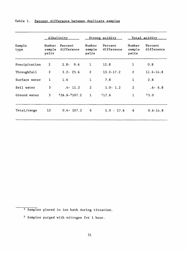
Table 1. Percent difference between duplicate samples
Alkalinity Strong aciditv Total acidity
Sample Number Percent Number Percent Number type sample difference sample difference sample
pairs pairs pairs
Precipitation 2 2.8-9.6 1 12.8 1
Throughfall 2 3.2-25.6 2 13.2-17.2 2
Surface water 1 1.6 1 7.8 1
Soil water 3 .4- 11.2 2 1.0- 1.2 2
Ground water 5 1 26.6- 2 107.2 1 l ll .6 1
Total/range 12 0.4-107.2 6 1.0-17.6 6
Percent difference
0.8
11.6-14.8
2.8
.6- 6.8
1 3.0
0.6-14.8
1 Samples placed in ice bath during titration.
2 Samples purged with nitrogen for 1 hour.
31

Table 2. Range of pH. specific conductance, and dissolved organic carbon for duplicate samples
[/iS/cm, microsiemens per centimeter at 25 degrees Celsius; mg/L, milligrams per liter; -- indicates no analytical data]
Sample type
precipitation
throughfall
surface water
soil water
ground water
Number sample pairs
1
2
1
3
5
PH (units)
4.5
4.1 - 4.4
3.5
4.0 - 4.1
4.7 - 5.0
Specific conductance (/iS/cm)
25
52 - 93
285
36 - 49
23 -261
Dissolved organic carbon (mg/L)
--
9.7 - 11
17.0
12.0 - 21
.5
.0
.0
32
SUMMARY
The limitations of some conventional techniques make the Gran technique
for alkalinity and acidity determinations a preferred method for the analysis
of low-pH, low-ionic-strength waters. The procedure described here is a
simplification of the Gran technique that can be performed easily and
inexpensively. The method is reliable for a variety of water sources, and
precision appears to increase with increased specific conductance and
decreased dissolved CO- content.
The successful application of Gran's technique to low-pH, low-ionic-
strength natural waters may be limited by the chemistry of a given water
sample. Meaningful interpretation of the analytical results depends on a full
understanding of the sample chemistry and the interferences that can occur.
In particular, interpretation of data from waters containing high levels of
organic matter and/or hydrolyzable metals may require knowledge of the groups
of organic acids and the particular metal species present. Geochemical
modeling combined with the Gran technique also should prove useful to
interpret analytical results.
33

REFERENCES CITED
Cosby, B. J., Hornberger, G. M., Galloway, J. N. , andWright, R. F., 1985, Modeling the effects of acid deposition: Assessment of a lumped parameter model of soil water and streamwater chemistry: Water Resources Research, v. 21, p. 51-63.
Drever, J. I., 1982, The geochemistry of natural waters: Englewood Cliffs, N.J., Prentice-Hall, Inc., 388 p.
Driscoll, C. T. , 1984, A procedure for the fractionation of aqueous aluminum in dilute acidic waters: International Journal of Environmental Analytical Chemistry, v. 16, p. 267-283.
Driscoll, C. T., and Bisogni, J. J., 1984, Weak acid/base systems in dilute acidified lakes and streams of the Adirondack region of New York State, in Schnoor, J. L., ed., Modeling of total acid precipitation impacts: Acid Precipitation Ser.- v. 9, Boston, Ma., Butterworth Publishers, p. 53-72.
Fishman, M. J., and Friedman, L. C., 1985, Methods for determination of inorganic substances in water and fluvial sediments: Techniques of Water-Resources Investigations of the United States Geological Survey, book 5, chap. Al, 626 p.
Galloway, J. N., Schofield, C. L., Hendry, G. K., Peters, N. E., andJohannes, Arland H., 1983, Lake acidification during spring snowmelt, in The intergrated lake-watershed acidification study: Proceedings of the ILWAS Annual Review Conference, EA 2827 Research Project 1109-5, Electric Power Research Institute, Palo Alto, Ca., p. 10-4 and 10-18.
Gran, Gunnar, 1952, Determination of the equivalence point in potentiometric titrations, Part II: The Analyst, v. 77, p. 661-671.
Greenberg, A. E., Connors, J. J., Jenkins, David, and Franson, M. A. H., eds., 1981, Standard methods for the examination of water and wastewater, 15th edition: American Public Health Association, Washington, D. C., 1134 p.
Hillmann, D. C., Morris, F. A., Potter, J. F., Cabell, K. G., and Simon, S. J., 1984, A methods manual for the National Surface Water Survey Project-- Phase I, February 15, 1984: United States Environmental Protection Agency, 127 p.
Johansson, Axel, 1970, Automatic titration by stepwise addition of equalvolumes of titrant, Part I. Basic principles: The Analyst, v. 95, p. 535-540.
Johnsson, P. A., and Lord, D. G., 1987, A computer program for geochemical analysis of acid-rain and other low-ionic-strength acidic waters: U.S. Geological Survey Water-Resources Investigations Report 87-4095, 42 p.
34

REFERENCES CITED--Continued
Keene, W. C., and Galloway, J. N., 1985, Gran's titrations: Inherent errors in measuring the acidity of precipitation: Atmospheric Environment, v. 19, p. 199-202.
Lee, Ying-Hua, and Brosset, Cyrill, 1978, The slope of Gran's plot: Auseful function in the examination of precipitation, the water-soluble part of airborne particles, and lake water: Water, Air, and Soil Pollution, v. 10, p. 457-469.
Lindberg, S. E., Coe, J. M., and Hoffman, W. A., 1984, Dissociation of weak acids during Gran plot free acidity titrations: Tellus, v. 36B, p. 186-191.
Lord, D. G., Barringer, J. L., Johnsson, P. A., Schuster, P. F., Walker, R. L., Fairchild, J. E., Sroka, B. N., and Jacobsen, Eric, 1990, Hydrogeochemical data from an acidic deposition study at McDonalds Branch in the New Jersey Pinelands, 1983-1986: U.S. Geological Survey Open-File Report 88-500, 132 p.
McKnight, Diane, Thurman, E. M., Wershaw, R. L., and Hemond, Harold, 1985, Biogeochemistry of aquatic humic substances in Thoreau's Bog, Concord, Massachusetts: Ecology, v. 66, p. 1339-1352.
McQuaker, N. R., Kluckner, P. D., and Sandberg, D. K., 1983, Chemical analysis of acid precipitation: pH and acidity determinations: Environmental Science and Technology, v. 17, p. 431-435.
Molvaersmyr, K., and Lund, W., 1983, Acids and bases in fresh waters.Interpretation of results from Gran plots: Water Resources, v. 17, p. 303-307.
Morel, F. M. M., 1983, Principles of aquatic chemistry: New York, N.Y., John Wiley and Sons, 446 p.
Oliver, B. G., Thurman, E. M., and Malcolm, R. L., 1983, The contribution of humic substances to the acidity of colored waters: Geochimica et Cosmochimica Acta, v. 47, p. 2031-2035.
Pagenkopf, G. K., 1978, Introduction to natural water chemistry:Environmental Science and Technology Series: v. 3, New York, N.Y., Marcel Dekker, Inc., 272 p.
Peters, D. G., Hayes, J. M., and Hieftje, G. M., 1974, Chemical separation and measurement, in Theory and practice of analytical chemistry: Philadelphia, Pa., W. B. Saunders, 379 p.
Plummer, L. N., Jones, B. F., and Truesdell, A. H., 1978, WATEQF--A FORTRAN IV version of WATEQ, a computer program for calculating chemical equilibrium of natural waters: U. S. Geological Survey Water-Resources Investigations Report 76-13, 61 p.
35

REFERENCES CITED--Continued
Stumm, Werner, and Morgan, J. J., 1981, Aquatic chemistry, 2nd edition: New York, N.Y., Wiley-Interscience, John Wiley and Sons, 780 p.
Thurman, E. M., 1985, Organic geochemistry of natural waters: Dordrecht, Martinus Nijhoff/Dr. W. Junk, 497 p.
Thurman, E. M., and Malcolm, R. L., 1981, Preparative isolation of aquatic humic substances: Environmental Science and Technology, v. 15, no. 4, p. 463-466.
Tyree, S. Y., 1981, Rainwater acidity measurement problems: Atmospheric Environment, v. 5, p. 57-60.
Weast, R. C., Astle, M. J., and Beyer, W. H., eds., 1988-1989, CRC Handbook of chemistry and physics, 69th edition: Boca Raton, Fla., CRC Press, Sections A - F.
36


![Theoretical considerations of static and dynamic ...prem.hanyang.ac.kr/down/Theoretical considerations of...Tribology International ] (]]]]) ]]]–]]] Theoretical considerations of](https://static.documents.pub/doc/80x56/5aa5e7d57f8b9a7c1a8e0cba/theoretical-considerations-of-static-and-dynamic-prem-considerations-oftribology.jpg)


